Maser Flare Simulations from Oblate and Prolate Clouds

Abstract

We investigated, through numerical models, the flaring variability that may arise from the rotation of maser clouds of approximately spheroidal geometry, ranging from strongly oblate to strongly prolate examples. Inversion solutions were obtained for each of these examples over a range of saturation levels from unsaturated to highly saturated. Formal solutions were computed for rotating clouds with many randomly chosen rotation axes, and corresponding averaged maser light curves plotted with statistical information. The dependence of results on the level of saturation and on the degree of deformation from the spherical case were investigated in terms of a variability index and duty cycle. It may be possible to distinguish observationally between flares from oblate and prolate objects. Maser flares from rotation are limited to long timescales (at least a few years) and modest values of the variability index ($\lesssim 100$), and can be aperiodic or quasi-periodic. Rotation is therefore not a good model for H₂O variability on timescales of weeks to months, or of truly periodic flares.

1 Introduction

This work is one of a series of publications that describe results of computational models of flares and variability in astrophysical masers arising from various possible mechanisms. The first paper in the series, Gray et al. (2018), hereafter Paper 1, considered variability due to rotation of a model cloud that had only small departures from spherical symmetry. After a brief general introduction, the present work will concentrate on the characteristics of flaring caused by the rotation of approximately spheroidal clouds of varying eccentricity.

Much recent observational interest has centered on correlations between infra-red variability in the continuum of young stellar objects (YSOs) and maser flares. Correlations of this type are particularly strong for flares in the 6.7-GHz maser transition of A-type CH₃OH. For example, in the YSO S255 NIRS 3, a 6.7-GHz flare is convincingly ascribed by Moscadelli et al. (2017) to an infra-red burst due to an accretion event associated with the host YSO. A reported 5-month delay between the infra-red and maser events, coupled with interferometric measurements of the maser and continuum positions requires information transfer at $>$6000 km s^-1: too fast for any mechanical transfer by shock waves that would not also destroy the maser molecules.

In the source NGC 6334I, continuum infra-red variability has been linked to maser flares in the three species OH (6 transitions), H₂O (22 GHz) and CH₃OH (3 transitions) (MacLeod et al., 2018). In this source there are various delay times associated with the different distances to regions of a VLBI map occupied by masers of each species. The maser flares were linked in this case to infra-red radiation produced by FU Ori-type accretion events in a massive protostar, or YSO, underlying the continuum source MMB1. It is interesting that some methanol 6.7-GHz spectral features were stable throughout the flare, whilst the flaring features occupied a new, redder, velocity range, offset by several km s^-1 from the main pre-flare spectrum.

While there are many instances of CH₃OH maser flares that are convingingly linked to infra-red variability in nearby continuum sources, the evidence for H₂O maser flares is more mixed. In the NGC 6334I source (MacLeod et al., 2018), water masers appear to share the radiatively driven variability of the other species. In some other sources, this may also prove to be the case: examples include IRAS18316-0602, where the H₂O flare appears to follow a brightening of a 2MASS source (Ashimbaeva et al., 2017; Sobolev et al., 2017), although a shock-driven variation in the pump rate has also been suggested (Lekht et al., 2018). In the IR source IRAS 16293-2422, H₂O maser flares have been more decisively linked to motions of shocked gas (Colom et al., 2016) on the basis of the spatial distribution of flaring objects along AU-scale chains that contain velocity gradients. Spectral shifts in velocity were observed as each successive object was shocked.

Shocks heat and compress gas, but do not guarantee the generation of rotational motion. However, given the very high Reynolds numbers in most interstellar flows, it is highly likely that post-shock gas will become turbulent in most shock-driven maser sources. Turbulent motion in turn drives the development of rotating structures and eddies that may have very small high-density cores (see for example H₂O masers in Cep A (Sobolev et al., 2018). Most 22-GHz H₂O masers are assumed to be pumped by a mainly collisional process following shock heating of the H₂O-bearing gas (Elitzur et al., 1989; Kaufman & Neufeld, 1996), so the rotation model of flares is probably more applicable to water masers than, for example, Class II methanol masers that are pumped mostly by infra-red radiation, with a consequent correlation of maser variability with that of the pumping radiation. Water maser flares are also more extreme in variability index so, if a rotation model is to be considered, it is very important to study significantly non-spherical clouds. Amplification by a rotating cloud in the line-of-sight has been specifically considered for a 22-GHz H₂O maser flare in W49N (Boboltz et al., 1998), with a surprisingly good fit to flux density, line width and centroid velocity via a simple model. That model, however, considered only an unsaturated rotating cloud between the observer and an already saturated maser source.

In Paper 1, we described a new 3-D code, specifically written to model maser sources, based on clouds of irregular shape. Saturation effects were treated in a self-consistent manner within the approximations of the model. The main approximations in Paper 1 were the use of a 2-level model with phenomenological pumping, an assumption of complete velocity redistribution (CVR) within the molecular response, an internally uniform cloud (or computational domain), and an approximately spherical distribution of triangulation nodes. In the current work, we lift the last of these restrictions in order to study the behaviour of strongly non-spherical clouds, noting that the finite-element discretisation of the domain will always lead to small asphericities, even if the node positions are selected from a spherical distribution.

The scientific driver for the current works is the need to model significantly larger flare amplitudes, observed from some masers in massive star-forming regions, than could be typically produced by the approximately spherical model in Paper 1 that yields ratios of maximum to minimum flux density at line centre of $\sim$3. If flare amplitude is the only consideration, then, for example, the monitoring data in Goedhart et al. (2004) shows that 68 of 372 spectral components, drawn from 54 6.7-GHz methanol maser sources, have a variability index of $<$3. We note that the variability index in Goedhart et al. (2004) is not simply the maximum to minimum flux density ratio in a chosen channel, but the point is that a substantial fraction of the observations cannot be explained in terms of a rotating pseudo-spherical cloud.

When considering 22-GHz H₂O masers, their variability behaviour is apparently more extreme: 43 sources were studied over 20 yr, with a cadence of 4-5 observations per year (Felli et al., 2007; Brand et al., 2007). A variability index used in Brand et al. (2007) is again defined differently from anything used so far but, judging from their Fig. 1b, almost all of the 43 sources are more strongly variable than the model from Paper 1. The issue of multiple definitions of the variability index is perhaps problematic: we note that three different variability indices have so far been introduced, which is potentially confusing. We discuss these definitions further in Section 4.2.

2 Modifications to the Model

The model, including triangulation, discretization, solution for the nodal populations, formal solution for the specific intensities seen by a distant observer, and the effects of rotation, remains largely the same as in Paper 1. The obvious difference in the current work is an additional shaping of the cloud, so that the point distribution that forms the domain becomes approximately either a prolate or an oblate spheroid. The shaping operation was inserted between the steps of point generation, into a volume-weighted spherical distribution as in Paper 1, and triangulation into finite elements. The shaping algorithm used in the current work was,

$$(x^{2}+y^{2})e^{\Gamma}+z^{2}e^{-2\Gamma}=1,$$ (1)

where $\Gamma$ is the deformation factor, a new input parameter of the code. If $\Gamma<0$, coordinates in the $xy$-plane are stretched, whilst the $z$-coordinate is compressed, leading to an oblate spheroidal cloud. Positive values of $\Gamma$ generate prolate clouds; if $\Gamma=0$, the original approximately spherical point distribution is preserved. The deformation in eq.(1) also conserves the volume of the domain (Sugano & Koizumi, 1998).

The code in Paper 1 ran on a single processor, but the version used in the present work was adapted to take advantage of multiple-processor architecture by using the OpenMP application program interface. Use of OpenMP allowed the parallel operation of 2-12 processors on desktop machines, and up to 16 processors on the coma parallel machine at the Jodrell Bank Centre for astrophysics.

In the course of this work, the Levenberg-Marquardt algorithm used in Paper 1 was replaced with a non-linear Orthomin(K) algorithm for the most time-intensive task of computing population solutions. The implementation of Orthomin(K) was based on Chen & Cai (2001) with an initialization method based on the two-point step size gradient method (Dai et al., 2002; Barzilai & Borwein, 1988). The Orthomin method was found to be less susceptible to convergence problems with increasing optical thickness (convergence to an accuracy of 10^-8 at depth multipliers of 20 or more is easily achievable with Orthomin, as opposed to significant problems at 13.0-13.5 with the Levenberg-Marquardt scheme). Perhaps a more significant advantage for larger domains is that the Orthomin method does not need to compute a Jacobian matrix, resulting in many fewer function calls.

3 Domains

The prolate and oblate domains were generated by applying distortions based on eq.(1) to the same original spherical distribution of points. The distortions were applied before DeLaunay triangulation to form finite elements. All domains were generated from the same sequence of 300 points, of which 234-249, dependent on $\Gamma$, survived the triangulation process to be incorporated into the final domain. A variety of distortion factors were applied, from mild ($|\Gamma|=0.1$) to strong ($|\Gamma|=0.6$). Control results were also obtained for a pseudo-spherical cloud with the same number of nodes and zero distortion.

In Figure 1 we show three views of a prolate domain with $\Gamma=+0.3$ (left-hand panel) with the observer’s viewing direction as marked. In all cases, the view along a specified cartesian axis is in the positive direction. The right-hand panel shows three views of an oblate domain with $\Gamma=-0.3$, also with observer’s viewing directions as marked.

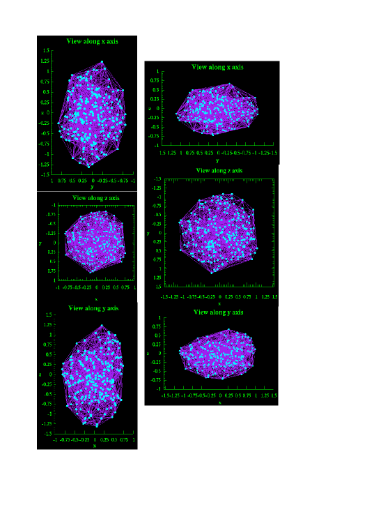
Figure 1: The left-hand panel shows three views of a prolate domain with $\Gamma=0.3$; the right hand panel shows the same views of an oblate domain with distortion $\Gamma=-0.3$. Cyan symbols mark nodal positions, and purple lines, the element edges.

Oblate clouds are likely to result from the shock compression of an initially spherical cloud, with the cloud flattened parallel to the shock front. An alternative generation mechanism is that of an initially spherical cloud with angular momentum, expanding into its surroudings and becoming rotationally flattened.

It is arguably more difficult to generate a prolate cloud, but one possibility is the expansion of an initially spherical cloud in a medium threaded by a magnetic field, a mechanism suggested for the shaping of the envelope of the OH/IR star OH26.5+0.6 (Etoka & Diamond, 2010). If the cloud medium is frozen to field lines that are dynamically dominant, then the cloud will be able to expand easily parallel to the field lines, but only with great difficulty perpendicular to the field. Certain hydrodynamic and magnetohydrodynamic instabilities can also lead to elongated cloud structures, for example the Rayleigh-Taylor instability and the sausage instability.

The ray-tracing algorithm was as used in Paper 1, so that, in the population (or inversion) solution, 1442 rays were traced from points on a celestial sphere-style source to every target node of the domain. The increased number of nodes compared to Paper 1, meant that somewhat larger total numbers of rays and saturation coefficients were generated. The celestial sphere source had the same specific intensity as in Paper 1: $i_{BG}=1.0\times 10^{-5}$, where $i_{BG}=I_{BG}/I_{sat}$, and $I_{sat}$ is the saturation intensity of the maser.

4 Results

First, we comment on the population solutions calculated for selected prolate and oblate clouds, with $|\Gamma|=0.3$, with particular emphasis on the differences from the pseudo-spherical cloud solution in Paper 1. Secondly, we discuss in detail the formal solutions, with simulations of rotation, that were used to generate light-curves for the clouds, as seen by a remote observer. Unlike the work in Paper 1, the present work allows the rotation axis of the domain to be selected independently of the long axis. In all cases, the observer’s plane is defined to be perpendicular to the rotation axis.

4.1 Nodal Solutions

Nodal solutions were generated in the same manner as in Paper 1: an initially very optically thin solution was obtained, and this solution (and at higher depths, several previous solutions) were then used as, or to predict, a first guess at an optically deeper solution. This process was originally continued until progress became very slow, at depth multipliers in the range 12.0-13.5. However, the adoption of the Orthomin(K) algorithm (see Section 2) has enabled us to consider results up to depth multipliers of at least 20. It should be noted from Fig. 1 that the actual maser depth implied by a given value of the depth multiplier is not the same as in the pseudo-spherical model in Paper 1. Whilst the shorter axis or axes still have a maximum chord length of approximately 1.8, the stretched axis, or axes, now have larger maximum chords of approximately 2.7 in the prolate case and 2.5 in the oblate case. A fixed value of the depth multiplier therefore corresponds to a generally higher maser depth than in the spherical case, with consequently greater optical thickness along some ray paths.

Population solutions are not the main focus of this work, but for completeness we show in Fig. 2 the distribution of the nodal inversions amongst 10 fractional bins for the prolate and oblate domains from Fig. 1 with the depth multiplier of 13.0. For comparison, we also show the histogram for the undistorted control case. In all cases, the background radiation was uniform at a level of 10^-5 with respect to the saturation intensity.

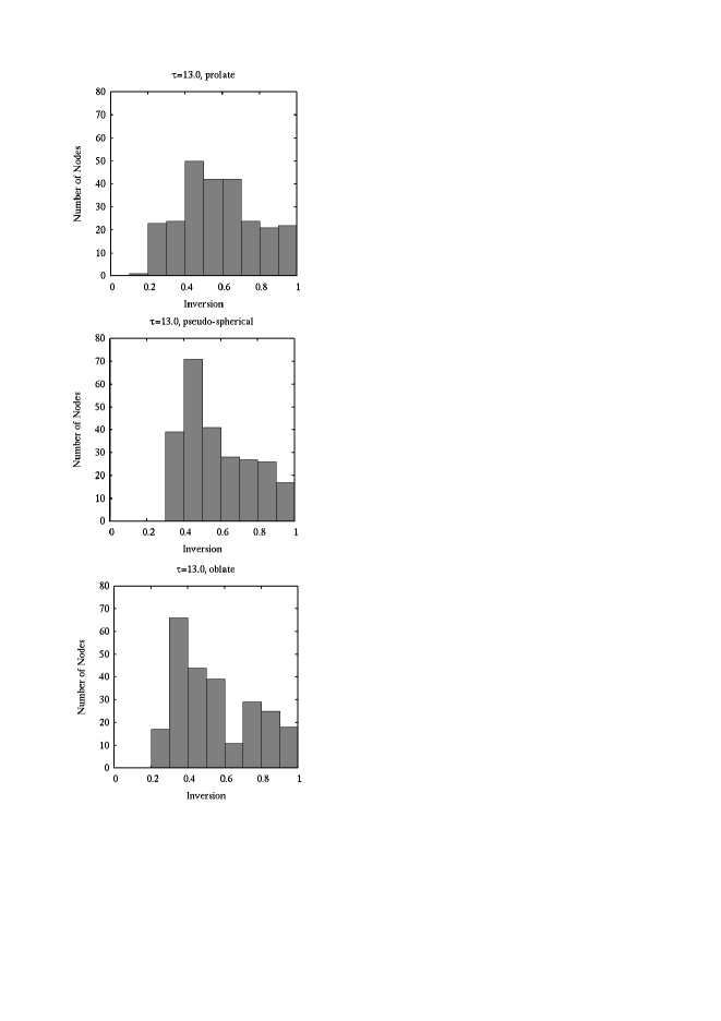
Figure 2: Histograms of the distribution of nodes between bins of fractional inversion with width 0.1. All three plots are at a depth multiplier of 13.0. The prolate model is at the top, the middle panel shows the pseudo-spherical model, and the oblate model is at the bottom.

In the prolate case, the most saturated node is at position $(0.2059,-0.2410,1.2362)$, placed well up the $z$-axis from the origin that is at the centre of the domain. This node is at a distance of 1.2762 from the origin, and is fairly easy to identify in both the top and bottom left-hand panels of Fig. 1. This node has only 0.196519 of its original inversion remaining. By contrast, the most saturated node in the pseudo-spherical model is only at a distance of 0.9938 from the origin, is significantly less saturated (0.31821 of the inversion remains) and its position, $(-0.4872,0.6433,0.5801)$, favours no particular axis. In the oblate case, the most saturated node is at $(-1.0880,-0.2870,0.0736)$, lying close to the $xy$-plane, and at a large distance from the origin (1.1276). As with the other models, the least saturated node is again close to the origin of the domain. All these results are consistent with expectations, and support the premise that the model is working correctly.

In Fig. 2, all the domains show significant evidence of saturation: the bin with the greatest number of nodes corresponds to a surviving inversion of 0.35 or 0.45. However, in both the prolate and oblate cases, the are more examples of highly saturated nodes, with the bin centered on an inversion of 0.25 well populated, and one node in the 0.15 bin in the prolate case. It can be argued that these results are as expected, since both the prolate and oblate models contain longer chords than are possible in the pseudo-spherical model, and a chord of length $\sim$2.5 is possible in the prolate model (see Fig. 1). All models continue to have a largely unsaturated core of $\sim$20 nodes (most right-hand bin in Fig. 2). It is also perhaps worth mentioning the more bi-modal nature of the oblate distribution, with a rather low number of nodes in the bin centered on an inversion of 0.65.

4.2 Formal Solutions and Rotation

In the work discussed here, formal solutions were obtained by solving the maser radiative transfer equation, as in Paper 1, with known nodal inversions. In each formal solution, the rays pass through the domain towards a specified observer’s position. We note that, in the case of the prolate cloud, an observer’s view along the long axis of the domain is strongly privileged, and expected to generate significantly stronger emission than any other viewpoint. Although a long axis can be determined in the other models, it will have many close rivals close to the $xy$-plane in the oblate model, and in arbitrary directions in the pseudo-spherical model.

As the current work deals with temporal variation resulting from cloud rotation, all the formal solutions were performed in the rotating frame of the cloud, which had no internal motion. Doppler corrections were then applied to the frequencies of the emitted rays to render these frequencies correct for a fixed observer viewing a rotating cloud. As in Paper 1, the dimensionless rotation rate corresponded to 1.162 Doppler widths unless otherwise stated.

The initial observer’s plane was chosen to be the $yz$-plane, and in Fig. 3 we show a specific intensity (maser brightness) map at five positions in this plane for the same three domains (prolate, pseudo-spherical and oblate) as used for Fig. 2. The colour palettes are the same in all panels of Fig. 3 to make the brightness variations between different viewpoints, and between the different domains, as clear as possible.

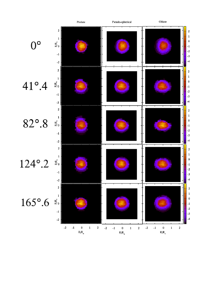
Figure 3: Images of the prolate domain (left-hand column), the pseudo-spherical domain (centre column) and the oblate domain (right-hand column). The five rows correspond to views with the observer’s position in the $yz$ plane at the angles marked, as measured from the North pole. The colour scale is the base-10 logarithm of the specific intensity in units of the saturation intensity.

All domains are shown to the same spatial scale, which leads to a slightly different background field in each case, since this has a size proportional to the long-axis of the domain in the sky-plane. In the case of the prolate cloud (left-hand column of Fig. 3, the top-most image has the observer viewing the North pole of the domain, almost along its long axis, and there is a small, but substantial, area that saturates the upper end of the colour table (bright yellow) representing specific intensities $>$1000 $I_{sat}$. In fact, the maximum intensity in this map is 1209$I_{sat}$. The image at 82°.8 in the prolate column is the closest to its thinnest possible presentation to the observer; here the peak brightnesses are only of order $100I_{sat}$. The brightest ray in fact has a specific intensity of 102$I_{sat}$. Therefore, rotation of the prolate domain, with this level of saturation, in a viewing plane that contains the long-axis is expected to show a maximum brightness variation of order of 10-20.

The pseudo-spherical cloud (middle column in Fig. 3) is expected to exhibit a variability of similar amplitude to the cloud in Paper 1, that is a ratio of maximum to minimum of $\sim$3. This is borne out by the sequence of maximum intensities, working down the middle column of 285, 411, 307, 393 and 511 times the saturation intensity. Clearly the expected amplitude of variation from the prolate cloud is considerably larger.

In the case of the oblate cloud (right-hand column of Fig. 3), the top-most image is the thinnest possible view of this cloud, viewed towards the North pole, or anti-parallel to the $z$-axis. As expected, the maximum brightness of 24.5$I_{sat}$ is much lower than for the same view of the prolate cloud (column 1, angle 0°) at 1209$I_{sat}$. The middle figure of the right-hand column (at 82°.8) shows the oblate cloud closest to its major plane, the $xy$-plane. The long axis of the cloud is expected to be in, or close to, this plane, so high brightness is expected. The largest specific intensity in this map was found to be 771 times the saturation value, so large amplitude variability is expected. In fact, this example is even more extreme, based on the ratio of maximum to minimum specific intensities found, than for the prolate case of the same $|\Gamma|$, axis of rotation and level of saturation.

In this work, we use from now on a definition of the variability index based on the ratio of the brightest specific intensity found at maximum light to the brightest found at minimum light. This definition, and two others mentioned in the Introduction, are set out mathematically in Appendix A. Our variability index specifically corresponds to eq.(3). The Brand et al. (2007) index is the more readily comparable of the other two to our models. For example, our spherical model from Paper 1 would have a variability index of $\sim$1.5 on the Brand et al. scale.

4.3 Variation of Viewing Plane

The images discussed in Section 4.2 correspond to a set of positions for a chosen observer’s plane. This plane should not be regarded as typical, so maser ligthcurves were plotted for a number of different observer’s planes (or rotation axes) to yield some statistical information, and suggest what an ‘average’ observer might record, rather than a very privileged one, who happens to view the domain rotating close to one of its principal axes. To this end, all three of the domains plotted in Fig. 3 were viewed from 1000 randomly oriented orbital planes, each perpendicular to an associated rotation axis. Note that in the models studied in the present work, the observer’s plane is always defined by the rotation axis, and oriented perpendicular to this axis: this is a consequence of converting from the rotating frame of the cloud, in which the population solution is calculated, to the fixed frame of the observer, in which the cloud is rotating, with appropriate Doppler corrections to the received frequencies.

5 Lightcurves

The principal results of the formal solutions, all of which simulate rotation in the present work, are lightcurves of maser peak specific intensity as a function of time. We define the peak specific intensity as the largest specific intensity found in a particular intensity file, where the intensity is a function of sky position and frequency. This parameter is comparable to the intensity of the brightest pixel found in any channel of an interferometer image cube from a VLBI observation. The time-base has twice the resolution of that in Paper 1: a 10-year rotation period is divided into 200 samples, each corresponding to a particular angle around one of the chosen orbital planes. As in Paper 1, all rotation is solid-body, and stability criteria strongly suggest that physical changes to the cloud imply that there is no point in following the rotation for more than one period; these models are most unlikely to be appropriate for periodic maser flares.

5.1 Prolate Cloud

We begin by considering the prolate cloud, and within this we choose conditions likely to produce extremes of variation. First we consider rotation about the $x$-axis, giving the $yz$-plane as the observer’s plane, as in Fig. 3. The long axis of the domain lies close to the $yz$-plane, and so, during one rotation, we expect to see two observer’s positions that would produce a specific intensity close to the largest possible value (see definition in Section 5 above). For the $yz$-plane, the light curve generated by cloud rotation is shown as the solid curve in Fig. 4, where the peak specific intensity rises to a maximum of 1877 times the saturation intensity at approximately half-way through the rotation. The lowest brightness found was 99.0 at position 144 of 200 (7.2 yr on the time base). The variability index is therefore 1877/99 $\simeq$ 19, compared to approximately 3 for the pseudo-spherical cloud in Paper 1.

Figure 4: Light curves of the maser emission produced by the rotating prolate cloud of deformation factor 0.3 in two extreme cases are shown: the solid curve results when the cloud is viewed from the $yz$-plane (rotation about the $x$-axis), and the dashed curve results when the observer’s plane is the $xy$-plane (rotation about the $z$-axis. The optical depth multiplier is 13.0.

By contrast, the second line in Fig. 4 (dashed) is the light-curve produced when the observer’s plane is the $xy$-plane, and rotation is about the $z$-axis. In this case, the observer is always viewing the cloud in a projection that is geometrically and optically close to the thinnest possible. Unsurprisingly, the peak specific intensities are generally lower than those following the solid curve (brightest value of 162), and the variability index is also substantially lower ($162/56\simeq 2.89$), since the cloud always presents an approximately constant range of thicknesses to the observer in this plane. This value of the variability index is consistent with that found for the pseudo-spherical object in Paper 1. Two possible observer’s views from the $xy$-plane appear in the top and bottom left-hand panels of Fig. 1. On the $y$-axis scale of Figure 4, the variability of the dashed curve is so weak that it is not possible to see much detail, so this light curve is re-plotted in Fig. 5 over a suitably smaller intensity range.

Figure 5: A magnification of the dashed ($xy$-plane) curve from Fig. 4, showing the detailed variability.

The light curve in Fig. 5 contains many peaks an troughs, that reflect the small-scale irregularity of the domain, rather than a strong pair that correspond to repeated presentation of the long axis towards the observer. There are no clear high or low states and no strong regularity in time. This indicates, as expected, that there are no strongly favoured viewpoints on this observer’s plane.

We now abandon the priveleged viewpoints that correspond to the light curves displayed in Fig. 4 and Fig. 5, and consider instead an average light curve that might correspond to a typical observer. To this end, formal solutions were computed for 1000 different, randomly oriented, rotation axes, each with 200 observer’s positions that correspond to time snapshots along the light curve. Note that in the present work, the rotation axes are truly random in space, whilst the similar work in Paper 1 used observer’s planes that all contained the long axis. The resulting light curves in the present work were then wrapped in time, so that in every case the highest intensity found was placed exactly half way along the time base, at 5 yr. The final light curve, shown in Fig. 6 is the mean over the 1000 random orientations after wrapping the time base; error bars on this curve indicate the sample standard deviation in the peak intensity. Unlike Paper 1, we plot only this one observable.

Figure 6: The average light curve resulting from the mean of 1000 rotations about randomly oriented axes for the prolate domain with deformation $\Gamma=0.3$ and optical depth multiplier of 13.0. Error bars indicate the sample standard deviation at each time.

The variability index of the averaged light curve is 6.92$\pm$0.15: considerably lower than the extreme variability case in Fig. 4, but larger than the spherical cloud in Paper 1, or the control example in the present work that has a variability index of 2.06$\pm$0.02.

5.2 Oblate Cloud

The oblate example cloud has a deformation factor of $-0.30$, so the magnitude is the same as for the prolate object consisdered in Section 5.1. The level of saturation is also the same (optical depth multiplier equal to 13.00). For an oblate cloud, any observer’s plane in which the object is presented edge-on to the observer is close to the extreme variability case, in the sense of the variability index defined in eq.(3). We chose to use the same rotation axis (the $x$-axis) as used in the prolate case. The observer’s plane is then the $yz$-plane, and example views include those shown in the right-hand column of Fig. 3. Rotation about this axis produces repeated edge-on and face-on views of the domain to the observer, and is a candidate for flaring events. The light curve is shown as the solid curve in Fig. 7. The variability index is equal to 48.0. We compare this to a case where the rotation axis is the $z$-axis (dashed curve in Fig. 7), and the observer’s view, from the $xy$-plane, is always close to edge-on. In the latter case, the maser emission has high intensity, but is only weakly variable, according to the variability index defined in eq.(3). The actual variability index in this case was 3.19. This value perhaps demonstrates the weakness of our simple definition of the variability index: although the index for the dashed curve is much lower on the basis of a maximum to minimum ratio, this curve is just as variable in terms of maximum to minimum difference.

Figure 7: Light curves for an oblate maser cloud of deformation factor $-0.30$ rotating about the $x$-axis (solid curve) and about the $z$-axis (dashed curve). In both cases, the optical depth multiplier is 13.0.

Moreover, in the case of rotation about the shorter ($z$) axis, an axis of length similar to the long axis of the domain is always pointing at the observer, whilst rotation about the $x$-axis only presents an axis of approximately this length towards the observer twice per rotation. This means that we expect the peaks of the solid curve to be only of similar intensity to the average intensity of the dashed light-curve (resulting from rotation about the $z$-axis). This is exactly what we see in Fig. 7. It should be possible to get a slightly brighter, highly variable, light curve by rotating about an axis exactly perpendicular to the long axis, but still close to the $xy$-plane, so that the long axis then does get presented half-periodically to the observer. However, even this latter case would not be expected to produce peaks of a significantly higher intensity than those of the dashed curve.

As in the prolate case, we proceed by considering the case of the light curve that would be observed by a more typical observer. As in Section 5.1 this is based on the average of 1000 observer’s planes, and consequently on the same number of randomly generated rotation axes. The resulting averaged light curve is shown in Fig. 8. Individual light curves were wrapped in time to place the maximum at 5 yr before averaging, also as in Section 5.1.

Figure 8: As for Fig. 6, but for the oblate domain with deformation factor $\Gamma=-0.3$. The $y$-axis scale is the same as in Fig. 6 for easy comparison.

Note that the height of the maximum is slightly higher than in the prolate case (see Fig. 6) and that the largest standard deviations are now concentrated towards the fainter parts of the light curve. The variability index is $8.22\pm 0.39$ so, at least on the basis of this very simple statistic, the oblate domain yields greater variability on average.

5.3 Effect of Saturation

To avoid viewing thousands of light-curves, further work will be based on some statistics that summarize most of the important information contained in the data. We use our definition of the variability index, as defined in eq.(3), and we also calculate the duty cycle, defined as the fraction of the full time base in which the intensity is above half the maximum found. Unless stated otherwise, these statistics were calculated from data based on 1000 observer’s planes, as in Fig. 6 and Fig. 8. Both quantities are calculated with a standard error that is plotted as a $y$-axis error bar in the relevant figures below.

In this section, we consider the standard prolate and oblate domains with $|\Gamma|=0.3$ and the pseudo-spherical control domain, but we now vary the degree of saturation by varying the optical depth multiplier from 7.0 (almost unsaturated, but still with an amplification factor of order 10⁶) to 20.0 (strongly saturated). Results for the average variability index (mean of 1000 light curves, based on randomly chosen rotation axes) is shown in Fig. 9.

Figure 9: The variability index (ratio of maximum to minimum peak brightness) as a function of optical depth multiplier for prolate, pseudo-spherical and oblate domains. Error bars show the standard error based on the 1000 realisations.

The key result is that, for the variability index as defined in eq.(3), increasing saturation reduces the index, eventually to a level similar to, but still larger than, the value of 2-3 typical of the pseudo-spherical domain. However, it should be noted that the actual maximum brightnesses at $\tau=20$ are of order 3000 I_sat, approximately 100 times larger than at $\tau=7$. From the observer’s point of view, it might therefore be more useful to consider a variability index based on the difference between maximum and minimum light, rather than the ratio.

In Fig. 10 we show the second statistic, the duty cycle. As in Fig. 9, this is based on the average of 1000 realisations. The curves plotted are for the pseudo-spherical domain and the prolate and oblate clouds with $|\Gamma|=0.3$.

Figure 10: The duty cycle (fraction of time for which the brightness is above half the maximum value) as a function of optical depth multiplier for prolate, pseudo-spherical and oblate domains.

Increasing saturation increases the duty cycle for all cloud types, and the effect is somewhat stronger for oblate than prolate domains, but much smaller than for the quasi-spherical case that goes through a rapid switch from low to high duty cycle at a depth multiplier of $\tau\sim 13$.

5.4 Effect of the Deformation Factor

In this section, we perform calculations similar to those in Section 5.3, but now we hold the optical depth multiplier at the standard value of $\tau=13.0$ whilst varying the deformation factor of the domain. We consider domains from $\Gamma=-0.6$ (extreme oblate) to $\Gamma=0.6$ (extreme prolate). The spherical example has $\Gamma=0$. Results are shown in Fig. 11 for the variability index, averaged over 1000 randomly selected rotation axes.

Figure 11: The variability index (ratio of maximum to minumum brightness) as a function of cloud deformation factor, $\Gamma$. Clouds become incresingly prolate with increasing $\Gamma$. Error bars show the standard error based on the 1000 realisations, and all models were run with an optical depth multiplier of 13.0.

We also show the effect of the deformation factor on the duty cycle in Fig. 12.

Figure 12: The duty cycle (see caption to Fig. 11) as a function of cloud deformation factor, $\Gamma$.

The duty cycle is a strong function of the deformation factor when the magnitude of this parameter is small. However, the behaviour is quite symmetric for the prolate and oblate domains, so the duty cycle is not a good statistic for distinguishing prolate and oblate clouds of the same $|\Gamma|$ observationally.

5.5 Execution Times

Calculation of the nodal solutions still dominates the execution time, as in Paper 1. However, adoption of the Orthomin($K$) algorithm (see Section 2) has reduced this time significantly, particularly at optical depth multipliers greater than $\sim$12. The new algorithm suffers from only a weak degredation in performance when strong saturation effects appear, and the code has been run to optical depth multipliers $>$30.

Under the DiRAC seed-corn grant dp110, better parallelisation of the code, and other efficiency improvements, have reduced the wall execution time of the version used in the present work to 28 s for a single iteration job on a desktop machine with twelve Intel Core i7-3930K CPUs, each rated at 3.20 GHz. This job requires initial reading of the domain data and ray route tracing in addition to the Orthomin solution. The same job run on the DiRAC DIAL machine at the University of Leicester took 12 s walltime on the development queue. The code on the DiRAC machine was compiled with the proprietory Intel compiler, whilst the desktop machine used the open-source GNU compiler.

6 Discussion

It is clear that both prolate and oblate maser clouds can produce flaring, and that the variability index, as judged from any of the definitions in Appendix A, can be significantly larger than for a pseudo-spherical cloud, given a favourable orientation of the rotation axis to the observer’s line of sight. As expected, the greatest variability occurs when the long axis of the domain, and an axis similar to the shortest possible, are sequentially presented to the observer. For a given depth multiplier, the greatest value of the variability index relates to a prolate domain with its long axis pointing directly at the observer. However, such an orientation is comparatively rare and, for a population of clouds with the same magnitude of deformation factor viewed at random angles, the variability index is comparable for oblate and prolate clouds. In fact, Fig. 11 shows a cross-over between $|\Gamma|=0.4$ and $0.5$, with oblate clouds having a higher variability index at lower values of $|\Gamma|$ and prolate clouds, at higher values.

From Fig. 9, we see that variability index is a decreasing function of optical depth multiplier. However, what is obvious, but not shown in this figure, is that the maximum brightness is a rising function of depth multiplier, particularly over the range of $7-12$, where saturation becomes increasingly important. Therefore, there is likely to be a substantial population of weakly saturated objects with high variability index that are only marginally detectable. For example an oblate object with $\Gamma=-0.3$ and depth multiplier of 7 (the lowest value plotted) has a maximum brightness of only 0.0053 times that of a similar object at depth 20.0. It is difficult to draw further conclusions without knowledge of how clouds are distributed in size and/or density in a particular source. However, for saturated clouds, high variability index (say $\gtrsim$10) requires clouds of large eccentricity (deformation factor magnitude).

The present work uses the peak specific intensity (see Section 5) as the main measure of maser output, and is therefore more closely related to interferometric observations than to single-dish spectra. However, spectroscopic counterparts to the data plotted in Fig. 6 and Fig. 8, also averaged over the 1000 realisations, are available, and we briefly consider the behaviour of a width parameter, defined as the ratio of the integrated flux to the peak flux density found in the spectrum. Measured in Doppler units, this width varied from 0.74 to 0.88 in the oblate cloud of $\Gamma=-0.3$ with a depth multiplier of 7.0. The prolate cloud of the same $|\Gamma|$ at this depth varied over the larger range of 0.68 to 0.93. However, for both cloud types, the width is anti-correlated with the flux density, as would be expected under the CVR approximation, where increased saturation does not lead to spectral re-broadening. At the higher depth multiplier of 13.0, both the typical width and its range of variation were reduced (oblate 0.593 to 0.637; prolate 0.596 to 0.640) but minimum width still correlated with maximum light.

The analysis in Section 5 offers some hope of distinguishing the variability of oblate and prolate clouds observationally. If a distribution of similar objects is present in a source, then a comparison of Fig. 6 and Fig. 8 shows that, near the peak of the averaged light curve, the standard deviation of the maximum brightness is significantly greater in the prolate case. It is probably best to concentrate on this part of the curve, as it is the most likely to be observed. However, the bias in the standard deviation is reversed in the troughs of the averaged light curves. There is also a significant kink in the wings of the peak in the prolate case (see Fig. 6). Duty cycle is generally higher for oblate clouds, particularly at large optical depths (see Fig. 10). For example, any flaring due to rotation of a $|\Gamma|=0.3$ cloud with a duty cycle above 0.2 is almost certainly oblate and strongly saturating. It is more difficult to say anything about the light curve of a single object, but a high brightness object with a low variability index is likely to be oblate and rotating close to edge-on with respect to the observer: in this orientation, all views of the object over one period have a similar geometrical depth.

Since cloud rotation is just one of many possible mechanisms for generating maser flares, the aim is to consider several more, and to present similar observational statistics by which mechanisms may be distinguished. One feature that cannot be explained by rotation, at least for a cloud that does not distort too much over a rotational period, is strong asymmetry in the lightcurve, particularly of a type that yields a longer time for the decay than for the rise on average. Preliminary studies indicate that superimposition of multiple clouds in the line of sight can produce significantly smaller duty cycles than the smallest found in Fig. 10 or Fig. 12, as well as significantly larger values of the variability index. However, we leave the details of classification methods to a future publication.

In a little more detail, Fig. 9 and Fig. 11 of the present work suggest that flares from cloud rotation are unlikely to produce a variability index in excess of 100. Timescales can be estimated from the simple stability criterion discussed in Paper 1. If the maximum rotation rate consistent with stability over one period is taken to be $\Omega_{max}=(2\beta/R)^{1/2}$ for pressure parameter $\beta$ and cloud radius, $R$, then the corresponding minimum period, or timescale more generally, is

$$P_{min}=2.18\times 10^{3}\left[\frac{\mu_{H}R_{AU}}{\alpha_{-3}n_{6}\sigma_{-20}T_{3}}\right]^{1/2}\;\;{\rm d},$$ (2)

where $\mu_{H}$ is the mean molecular mass of the gas external to the cloud in hydrogen atom units, $R_{AU}$ is the cloud radius in astronomical units, $\alpha_{-3}$ is in units of 10^-3, $\sigma_{-20}$ is the collision cross-section in units of 10^-20 m², $n_{6}$ is the number density of the external gas in units of cm^-3, and $T_{3}$, the temperature of the external gas in units of 1000 K. Allowing for favourable values of the parameters in eq.(2), we should therefore expect timescales of order a few years or more in addition to modest values of the variability index. Rotation can therefore already be ruled out as a mechanism for flares with timescales of weeks to months.

7 Conclusions

Rotation of irregular, approximately spheroidal, clouds provides a mechanism for maser flares of modest variability index and long timescale. The variability index ranges from a few to $\lesssim$100 if the index is the one defined in eq.(3). Shorter timescales than $\sim$1 yr are excluded on the grounds of stability of the cloud, as are truly periodic flares. Given these restrictions, rotation is more suited to possibly providing some of the variability associated with Class II methanol masers than with very bright and rapid H₂O maser flares.

Both prolate and oblate objects can produce strong flares. The averaged light curves of the two types are quite strong functions of the degree of saturation in the cloud and of the degree of deformation, with more extreme objects exhibiting stronger variability. Variability declines with increasing saturation for an object of given eccentricity, but the highly variable, weakly saturating objects are typically hundreds of times less bright, and so less likely to be visible. Detailed differences in the average behaviour of well-chosen statistics may enable us to distinguish between the maser emission from oblate and prolate clouds.

The choice of variability index used in this work is arguably not the best possible, and some discussion over the most useful definition of this index for maser variability studies is desirable.

Appendix A Variability Indices

Unfortunately, whilst any study of maser variability needs some measure of the strength of that variability, there does not at present seem to be any accepted standard for such a measure, or index. In Section 4.2, three different variability indices were introduced, all of which are defined below. In Paper 1 we used the index,

$${\cal V}_{1}=S_{max}/S_{min},$$ (3)

where $S$ is a flux or intensity measure, and $S_{max}$ and $S_{min}$ denote the respective maximum and minimum values of that measure found in a given time interval. In Paper 1, three different quantites were used for $S$: the maximum pixel brightness (specific intensity) found in an image; the flux density in the central spectral channel and the frequency-integrated flux. For simplicity, only the first of these measures is used for $S$ in the present work.

In their study of 22-GHz H₂O maser variability, Brand et al. (2007) use the variability index,

$${\cal V}_{B}=F_{max}/\bar{F},$$ (4)

where $F$ is the flux density (in a specified channel) and $\bar{F}$ is its mean value over the duration of the observing programme.

In their extensive variability survey of 6.7 GHz methanol masers, Goedhart et al. (2004) use the variability index definition, calculated for a specific velocity or frequency channel, of

$${\cal V}_{G}=\frac{\sum_{j=1}^{J}(F(t_{j})-\bar{F})^{2}-\sum_{j=1}^{J}(F_{N}(t_{j})-\bar{F}_{N})^{2}}{\bar{F}^{2}},$$ (5)

where $t_{j}$ is the time of the $j$th sample in a series of $J$ observations. $F(t_{j})$ is the flux density at time $t_{j}$ and $\bar{F}$ is the mean flux density over all $J$ observations. Quantities with the subscript $N$ are calculated from a noise channel, which implies a channel without maser emission. This definition was adopted from earlier work on Cepheid variables by Stetson (1996).

The present authors have taken the liberty of squaring the mean flux density in the denominator of eq.(5) in order to yield a dimensionless variability index: the original in equation 1 of Goedhart et al. (2004) has units of flux density as written, but the index does appear dimensionless in their tables, and it is also in Stetson (1996), though with a different normalization.

References

- Ashimbaeva et al. (2017) Ashimbaeva N. T., Platonov M. A., Rudnitskij G. M., Tolmachev A. M., 2017, The Astronomer’s Telegram, 11042
- Barzilai & Borwein (1988) Barzilai J., Borwein J. M., 1988, IMA Journal of Numerical Analysis, 8, 141
- Boboltz et al. (1998) Boboltz D. A., Simonetti J. H., Dennison B., Diamond P. J., Uphoff J. A., 1998, ApJ, 509, 256
- Brand et al. (2007) Brand J., Felli M., Cesaroni R., Codella C., Comoretto G., Di Franco S., Massi F., Moscadelli L., Nesti R., Olmi L., Palagi F., Palla F., Panella D., Valdettaro R., 2007, in Chapman J. M., Baan W. A., eds, IAU Symposium Vol. 242 of IAU Symposium, A 20-year H2O maser monitoring program with the Medicina 32-m telescope. pp 223–227
- Chen & Cai (2001) Chen Y., Cai D., 2001, App. Maths. & Computation, 124, 351
- Colom et al. (2016) Colom P., Lekht E. E., Pashchenko M. I., Rudnitskii G. M., Tolmachev A. M., 2016, Astronomy Reports, 60, 730
- Dai et al. (2002) Dai Y., Yuan J., Ya-Xiang Y., 2002, Computational Optimization and Applications, 22, 103
- Elitzur et al. (1989) Elitzur M., Hollenbach D. J., McKee C. F., 1989, ApJ, 346, 983
- Etoka & Diamond (2010) Etoka S., Diamond P. J., 2010, MNRAS, 406, 2218
- Felli et al. (2007) Felli M., Brand J., Cesaroni R., Codella C., Comoretto G., di Franco S., Massi F., Moscadelli L., Nesti R., Olmi L., Palagi F., Panella D., Valdettaro R., 2007, A&A, 476, 373
- Goedhart et al. (2004) Goedhart S., Gaylard M. J., van der Walt D. J., 2004, MNRAS, 355, 553
- Gray et al. (2018) Gray M. D., Mason L., Etoka S., 2018, MNRAS, 477, 2628
- Kaufman & Neufeld (1996) Kaufman M. J., Neufeld D. A., 1996, ApJ, 456, 250
- Lekht et al. (2018) Lekht E. E., Pashchenko M. I., Rudnitskii G. M., Tolmachev A. M., 2018, Astronomy Reports, 62, 213
- MacLeod et al. (2018) MacLeod G. C., Smits D. P., Goedhart S., Hunter T. R., Brogan C. L., Chibueze J. O., van den Heever S. P., Thesner C. J., Banda P. J., Paulsen J. D., 2018, MNRAS, 478, 1077
- Moscadelli et al. (2017) Moscadelli L., Sanna A., Goddi C., Walmsley M. C., Cesaroni R., Caratti o Garatti A., Stecklum B., Menten K. M., Kraus A., 2017, A&A, 600, L8
- Sobolev et al. (2017) Sobolev A. M., Bisyarina A. P., Tatarnikov A. M., Antokhin I., Volvach A. E., 2017, The Astronomer’s Telegram, 10788
- Sobolev et al. (2018) Sobolev A. M., Moran J. M., Gray M. D., Alakoz A., Imai H., Baan W. A., Tolmachev A. M., Samodurov V. A., Ladeyshchikov D. A., 2018, ApJ, 856, 60
- Stetson (1996) Stetson P. B., 1996, PASP, 108, 851
- Sugano & Koizumi (1998) Sugano S., Koizumi H., 1998, Microcluster Physics. Springer Series in Materials Science, Springer, Berlin