Calculation of non-universal thermodynamic quantities within self-consistent non-perturbative functional renormalization group approach

Abstract

A self-consistent renormalization scheme suitable for the calculation of non-universal quantities in $n$-vector models with pair spin interactions of arbitrary extent has been suggested. The method has been based on the elimination of the fluctuating field components within the layers defined by the layer-cake representation of the propagator. The non-perturbative renormalization group (RG) equations has been solved in the local potential approximation. Critical temperatures of the $n=1-3$ vector spin models on cubic lattices have been calculated in excellent agreement with the best known estimates. Several critical amplitudes and the magnetisation curve of the Ising model on the simple cubic lattice calculated within the approach compared well with the values from literature sources. It has been argued that unification of the method with cluster techniques would make possible the treatment of realistic lattice models with multi-spin interactions and describe in a unified framework the phase transitions of any kind. Besides the RG equations the layer-cake technique can be used in the exact partial renormalization of the local interactions in the functional lattice Hamiltonians. This procedure reduces the strength of the interactions which in some cases can make them amenable to perturbative treatment.

Keywords: renormalization group, layer-cake representation, local potential approximation, $n$-vector spin models, cubic lattices, critical temperatures, critical amplitudes

1 Introduction

Phase transitions in many-body systems are formally defined as the points where derivatives of the free energy with respect to thermodynamic variables become singular. Microscopic Hamiltonians are usually assumed to be smooth functions of their parameters, so calculations of the free energy based on series expansion in the powers of the Hamiltonian or of its parts to any finite order cannot exhibit the singularities. This means that phase transitions can be described only within non-perturbative approaches capable of calculating the free energy to all orders in the Hamiltonian which in general is a very difficult task.

The problem simplifies in the case of lattice models where the infinite system can be modelled by a finite cluster of sites. The partition function of the cluster can be calculated exactly to all orders in the interaction parameters and with suitable measures taken to embed the cluster into the infinite system remarkably accurate results can be obtained with the use of relatively small clusters (see [1, 2, 3, 4] and references to earlier literature therein). The cluster approximation is systematic in the sense that it can be indefinitely improved by enlarging the cluster size so in principle it presents a viable alternative to the series expansions as a general approach to the many-body problems with strong interactions.

From the standpoint of the phase transitions theory the main drawback of the cluster approach is its inability to adequately treat the long-range fluctuations [3, 4] that are paramount to the description of the continuous transitions and the critical points. As is known, the critical behaviour can be successfully described within the renormalization group (RG) approach [5]. Extensive studies in the framework of the perturbation theory have revealed many aspects of the universal behaviour in the vicinity of the critical point [5, 6, 7]. In particular, accurate values of the critical exponents and the critical amplitude ratios have been calculated which for many practical purposes can be considered as exact and by virtue of the universality can be used in interpretation of experimental data in a variety of systems. But for a concrete system one is also interested in non-universal quantities such as the absolute values of the critical amplitudes and the critical temperature as well as in the behaviour beyond the critical region. A natural way of achieving this would be the development of suitable non-perturbative RG techniques in order to profit from the well developed description of the universal behaviour. Besides, the RG approach is known to be completely general and may be used also away from the critical point [5]. The non-perturbative approximations to the exact RG equations have been extensively studied over the past decades but existing calculations of the system-specific non-universal quantities within this approach did not lead to development of a general systematic technique (a discussion of this problem and an extensive bibliography on the non-perturbative RG may be found in [8]).

The aim of the present paper is to suggest a renormalization scheme closely related to the functional cluster techniques introduced in [9, 3]. The ultimate goal would be to develop a non-perturbative RG approach that could be unified with the cluster method in such a way as to make possible systematic improvement of the accuracy thus making it also self-contained. Besides, the unification would make possible dealing with non-local many-body interactions which arise, e.g., in the realistic models of alloys [1, 10]. However, in the present paper only the RG equations will be considered in detail because, on the one hand, the feasibility of such a unification discussed in section 7 is in principle rather straightforward, but on the other hand, it would require extensive additional calculations requiring a separate study [11]. Besides, the local potential approximation (LPA) that will be used in the implementation of the RG scheme is not restricted to lattice models [12, 13, 14] so the results obtained in the present paper may be straightforwardly applied to the models in continuous space as well.

2 Definitions and notation

The partition functions of the lattice $n$-vector model can be represented in the functional integral form as

$$Z[{\bf h}]=\int D{\bf s}e^{-H[{\bf s}]+{\bf h}_{i}\cdot{\bf s}_{i}}$$ (1)

where the real fluctuating $n$-vector field ${\bf s}_{i}$ and the external source field ${\bf h}_{i}$ are defined at the sites $i$ of a periodic $d$-dimensional lattice of size $N$; $D{\bf s}=\prod_{i}d{\bf s}_{i}$ and $H$ is a dimensionless Hamiltonian. To simplify notation summation over repeated discrete subscripts corresponding to the lattice sites and the $n$-vector components will be implicitly assumed throughout the paper. Boldface characters and the dot products will refer both to $d$- and $n$-dimensional vectors, though for simplicity the site coordinates, such as $i$, will not be boldfaced.

The connected correlation functions (CFs) of the field can be found by differentiation of their generating functional $\ln Z[{\bf h}]$ with respect to the source field ${\bf h}$ [15]. Two CFs will be calculated in the present paper : the magnetisation $m_{\sigma i}$ equal to the average

$${m}_{\sigma i}\equiv\langle s_{\sigma i}\rangle=\left.\frac{\partial\ln Z[{\bf h}]}{\partial h_{\sigma i}}\right|_{\bf h=0},$$ (2)

where the subscript $\sigma=1,\dots,n$ numbers the vector components, and the connected part of the pair CF $G^{R}_{ij}$

$$G_{ij}^{R}=\left.\frac{\partial^{2}\ln Z[{\bf h}]}{\partial h_{\sigma i}\partial h_{\sigma j}}\right|_{\bf h=0}=\langle{s}_{\sigma i}{s}_{\sigma j}\rangle-{m}_{\sigma i}{m}_{\sigma j}.$$ (3)

Though in general non-trivial pair correlations between all field components may exist, only the diagonal in $\sigma$ CF defined in (3) will be used in the present study. Besides, because only fully $O(n)$ symmetric Hamiltonians will be considered below and only the symmetric phase treated in the $n>1$ case all diagonal CFs will be equal and the subscript $\sigma$ may be omitted; the spontaneous symmetry breaking will be discussed only for the $n=1$ Ising model in which case the subscript is also superfluous. The superscript $R$ in (3) and below will mark all fully renormalized quantities.

In the present paper we will deal with Hamiltonians of the following general form

$$H[{\bf s}]=\frac{1}{2}{s}_{\sigma i}\epsilon_{ij}{s}_{\sigma j}+H_{I}[{\bf s}].$$ (4)

where the first part describes pair interactions between $n$-vectors at different sites while the interaction part $H_{I}$ will be assumed to be local to the sites; matrix $\hat{\epsilon}=||\epsilon_{ij}||$ does not depend on $\sigma$ because of the $O(n)$ symmetry. It is important to note that both terms on the right hand side (r.h.s.) of (4) may contain local quadratic terms which may be used to choose them in such a way that the lattice Fourier transform of ${\epsilon}_{ij}$ behaved as

$$\epsilon({\bf k})|_{{\bf k}\to 0}\propto{\bf k}^{2},$$ (5)

which is convenient for implementation of the RG techniques in the case of homogeneous (ferromagnetic) ordering [5] which will be assumed throughout the paper.

The spin models differ from the general $n$-vector case in that the length of vectors ${\bf s}_{i}$ is fixed which for definiteness will be chosen to be equal to unity [16]. In the functional integral representation (1) this can be accounted for by the product of the Dirac’s delta-functions as

$$e^{-H_{I}}=\prod_{i}\delta({\bf s}_{i}^{2}-1)=\lim_{u_{4}\to\infty}\left({\frac{u_{4}}{\pi}}\right)^{N/2}e^{-u_{4}\sum_{i}({\bf s}_{i}^{2}-1)^{2}}$$ (6)

where the second equality shows that this case can also be formally described by Hamiltonian (4) with infinitely strong local quartic interactions. An important advantage of the layer-cake renormalization scheme is that such the treatment of such interactions is not more difficult than of local interactions of finite strength (see section 4.2 below).

3 The functional-differential formalism and the self-consistency

A general self-consistent approach to statistical models within the functional formalism was amply discussed in [9, 3, 4, 11] so below only short explanations will be given of the formulas that will be needed in subsequent calculations.

The Fourier transformed exact (i.e., fully renormalized) CF (3) may be cast in the form

$$G^{R}({\bf k})=\frac{1}{\epsilon({\bf k})+r^{R}({\bf k})}$$ (7)

where $r^{R}$ is the exact mass operator. As is seen, (7) expresses one unknown function through another unknown function so a natural question arises why complicate matters by introducing additional quantity that is equivalent to the existing one? The answer is that in many cases the mass operator can be approximated by a constant thus making its self-consistent calculation simpler because one would need to solve an equation for a single number instead of a function. The two cases pertinent to this study are the single-site approximation (SSA) and the LPA:

$$r^{R}_{ij}\simeq r\delta_{ij}\mbox{\ (SSA)}$$ (8)

$$r^{R}({\bf k})\simeq r^{R}({\bf k=0})=r\mbox{\ (LPA)}.$$ (9)

As is seen, in both cases the mass operator is site-diagonal and/or momentum-independent so the approximate CF in both cases has the form

$$G({\bf k})=\frac{1}{\epsilon({\bf k})+r}.$$ (10)

The difference lies in the self-consistency conditions which $r$ must satisfy in each case. It is pertinent to note that this form of renormalized CF implies that the critical exponent $\eta$ is equal to zero because $r=0$ at the critical point and from (5) it follows that $G\sim 1/{\bf k}^{2}$ as $|{\bf k}|\to 0$. This deficiency of the LPA is well known makes the approximation suitable for models in $d\geq 3$ [14]. It is for this reason that only 3D systems will be considered in the explicit calculations below.

Equations for a self-consistent calculation of $r$ can be derived with the help of the ambiguity in the separation in the quadratic and the interaction parts in (4) mentioned in the previous section [9, 3, 4, 11]. By adding and subtracting from the two parts of $H$ on the r.h.s. of (4) a local quadratic term $r{\bf s}_{i}\cdot{\bf s}_{i}/2$ the partition function (1) may be cast in the functional-differential form [17, 15, 9, 3]

$$Z[{\bf h}]=\det(2\pi\hat{G})^{n/2}\left.\exp\left(\frac{1}{2}{\partial_{\phi_{\sigma}}}\hat{G}{\partial_{\phi_{\sigma}}}\right)e^{\frac{r}{2}{\boldsymbol{\phi}}_{i}\cdot{\boldsymbol{\phi}}_{i}-H_{I}[{\boldsymbol{\phi}}]+{\bf h}_{i}\cdot{\boldsymbol{\phi}}_{i}}\right|_{\boldsymbol{\phi}=0}$$ (11)

which can be reduced to (1) with the use of the operator identity

$$\det(2\pi\hat{G})^{n/2}\exp\left(\frac{1}{2}{\partial_{\phi_{\sigma}}}\hat{G}{\partial_{\phi_{\sigma}}}\right)=\int D{\bf s}\exp\left(-\frac{1}{2}{s}_{\sigma}\hat{G}^{-1}{s}_{\sigma}+{\bf s}_{i}\cdot\partial_{{\boldsymbol{\phi}}_{i}}\right).$$ (12)

To further shorten expressions with summations over the sites a vector-matrix notation has been introduced in (11) and (12) with the $N$-component vectors defined as ${\bf s}=[{\bf s}_{i}]$ and the $N\times N$ matrix $\hat{G}=||G_{ij}||$ is the propagator (10) in the lattice coordinates.

The source field ${\bf h}$ in (11) can be disentangled from the action of the second-order differential operator to give [3]

$$Z[{\bf h}]=e^{\frac{1}{2}{h_{\sigma}}\hat{G}{h_{\sigma}}}e^{{h_{\sigma}}\hat{G}\partial_{\phi_{\sigma}}}\left.S[{\boldsymbol{\phi}}]\right|_{\boldsymbol{\phi}=0}=e^{\frac{1}{2}{h_{\sigma}}\hat{G}{h_{\sigma}}}S[{\bf h}\hat{G}]$$ (13)

where

$$S[{\boldsymbol{\phi}}]=\det(2\pi\hat{G})^{n/2}\exp\left(\frac{1}{2}{\partial_{\phi_{\sigma}}}\hat{G}{\partial_{\phi_{\sigma}}}\right)e^{\frac{r}{2}{\boldsymbol{\phi}}_{i}\cdot{\boldsymbol{\phi}}_{i}-H_{I}[{\boldsymbol{\phi}}]}\equiv e^{-U^{R}[{\boldsymbol{\phi}}]}$$ (14)

is the generating functional of the S-matrix [17, 15, 9, 3] and $U^{R}$ its connected part.

According to (3) the pair CF can be found from (13) as

$$G^{R}_{\sigma ij}=\left.\frac{\partial^{2}\ln Z[{\bf h}]}{\partial h_{\sigma i}{\partial h_{\sigma j}}}\right|_{\bf h=0}=G_{ij}-G_{il}\left.\frac{\partial^{2}U^{R}[{\boldsymbol{\phi}}]}{\partial\phi_{\sigma l}{\partial\phi_{\sigma l^{\prime}}}}\right|_{\boldsymbol{\phi}=0}G_{l^{\prime}j}$$ (15)

which establishes a relation between $G^{R}$ and $G$ that can be used to derive the self-consistency equation. Though relation (15) is exact, the simple form of $G$ (10) does not make possible its identification with $G^{R}$ by simply setting the second term on the r.h.s. to zero. The equality $G^{R}=G$ can be satisfied only approximately and the SSA is obtained by requiring that all matrices in (15) are diagonal. In this case the second term in (15) will vanish provided the second derivative of $U^{R}$ will be equal to zero when $l=l^{\prime}$. This approximation is adequate when the correlations are strongly localized which means large $r$ or small correlation length $\xi\propto r^{-1/2}\ll 1$ in the lattice units (l.u.). Explicit expression for $U^{R}$ in this case can be found from (14) which factorizes into the product of identical functions of ${\boldsymbol{\phi}}_{i}$ [9]. Correspondingly, $U^{R}$ becomes the sum of single-site contributions which can be used to derive the SSA equation.

SSA gives a reasonably accurate description of the first order phase transitions but fails near the critical points [9, 3, 4] where the LPA condition (9) is more appropriate because it approximates the CF in the large wavelength limit suitable for the critical region. Formally (9) holds when the Fourier transform of the second derivative of $U^{R}$ in (15) term is equal to zero:

$$\left.\frac{\partial^{2}U^{R}[{\boldsymbol{\phi}}]}{\partial\phi_{\sigma,{\bf k}}{\partial\phi_{\sigma,{\bf-k}}}}\right|_{{\boldsymbol{\phi}=0},{\bf k=0}}=0.$$ (16)

where

$${\phi}_{\sigma,{\bf k}}=N^{-1/2}\sum_{j}e^{-\mathrm{i}j\cdot{\bf k}}{\phi}_{\sigma j}.$$ (17)

The effective potential $U^{R}$ in the long wavelength limit ${\bf k\to 0}$ can be calculated with the use of the self-consistent RG equation derived below.

4 The renormalization scheme

In the functional-differential formalism the RG is naturally introduced through (14) cast in the form

$$e^{-U^{R}[{\boldsymbol{\phi}}]}=\exp\left(\frac{1}{2}\sum_{\bf k}\partial_{{\phi}_{\sigma,{\bf k}}}G({\bf k})\partial_{{\phi}_{\sigma,{\bf-k}}}\right)e^{-U^{0}[{\boldsymbol{\phi}}]}$$ (18)

where

$$U^{0}[{\boldsymbol{\phi}}]=-\frac{r}{2}{\boldsymbol{\phi}}_{i}\cdot{\boldsymbol{\phi}}_{i}+H_{I}[{\boldsymbol{\phi}}]+\mbox{(f.i.t.)}.$$ (19)

Here general notation “(f.i.t.)” has been introduced for the field-independent terms originating from various normalization constants and may also depend on physical quantities. For example, as follows from (14), in (19) $\mbox{(f.i.t.)}=-\ln\left[\det(2\pi\hat{G})^{n/2}\right]$. Such terms are necessary for the calculation of the absolute value of the free energy but it will not be calculated in the present paper such terms for brevity will be designated by the acronym. In case of necessity they can be easily recovered.

The continuous renormalization procedure (discrete renormalization can be performed similarly) in the functional-differential formalism proceeds as follows. First the exponentiated operator in (18) is represented as an integral over some parameter $t$ of commuting $t$-dependent operators. For definiteness the parameter can be chosen to vary from $t=0$ to some maximum value $t_{end}$ with $t=0$ corresponding to the “bare” functional $U^{0}$ with the fully renormalized $U^{R}$ being recovered and at $t=t_{end}$. Because of the commutativity the integration can be stopped at any $0\leq t\leq t_{end}$ which defines a partially renormalized effective potential $U[{\boldsymbol{\phi}},t]$. Obviously that its form will depend on the infinitesimal operators used which can be defined in an infinite number of ways with different choices corresponding to different renormalization schemes. Though $U^{R}$ at the end of the renormalization should be the same, the RG flow will strongly depend on the scheme chosen and in approximate calculations may significantly influence the computational efficiency and the accuracy of the results obtained.

The main goal of the present paper is to introduce a renormalization scheme that in the case of lattice models has shown good accuracy in the calculation of non-universal quantities in 3D $n$-vector models (see below) and should be suitable for renormalization of models with very strong local potentials, such as the formally infinitely strong interactions in the spin models (6). The scheme is a lattice generalization of the rotationally invariant version of [18] which has been achieved via the use of the layer-cake representation [19] for the propagator (10).

4.1 The layer-cake representation [19]

The representation is defined for non-negative functions so below we will assume that $G({\bf k})>0$. In this case the layer-cake representation can be introduced through a simple identity valid for any positive function

$$G({\bf k})=\int_{0}^{G({\bf k})}1\,dt^{\prime}=\int_{0}^{\infty}\theta[G({\bf k})-t^{\prime}]dt^{\prime}.$$ (20)

Substituting this in (18) we obtain the necessary split of the operator into infinitesimal parts to be used in the further incremental renormalization. As explained above, the partly renormalized effective interaction $U[{\boldsymbol{\phi}},t]$ in this case satisfies the equation

$$e^{-U[{\boldsymbol{\phi}},t]}=\exp\left(\frac{1}{2}\sum_{\bf k}\int_{0}^{t}\theta[G({\bf k})-t^{\prime}]dt^{\prime}\partial_{{\phi}_{\sigma,{\bf k}}}\partial_{{\phi}_{\sigma,{\bf-k}}}\right)e^{-U^{0}[{\boldsymbol{\phi}}]}$$ (21)

or, equivalently, the functional-differential evolution equation

$$U^{\prime}_{t}=\frac{1}{2}\sum_{\bf k}\theta[G({\bf k})-t]\left(\partial_{{\phi}_{\sigma,{\bf k}}}\partial_{{\phi}_{\sigma,{\bf-k}}}U-\partial_{{\phi}_{\sigma,{\bf k}}}U\partial_{{\phi}_{\sigma,{\bf-k}}}U\right).$$ (22)

with the initial condition $U[{\boldsymbol{\phi}},t=0]=U^{0}[{\boldsymbol{\phi}}]$. Equation (22) has a typical structure of the most essential part of the exact RG equations derived, e.g., in [5, 13] (see extensive bibliography to more recent literature in [8]) and differs only in the specific choice of the function $\theta$ and in the absence of the change of variables usually made to obtain RG equation in the scaling form. This change can be easily performed in the case of necessity but we mostly will not use it because it introduces into the equation the largest critical exponent $d$ which is completely trivial by simply reflecting the fact that the free energy grows with the linear system size $L$ as $L^{d}$. However, being the largest Lyapunov exponent of the equation it severely hampers its numerical stability.

The difference of the layer-cake renormalization scheme from the conventional RG procedure is that in (22) the field variables are eliminated by infinitesimal layers in the direction orthogonal to that in the Wilsonian renormalization, as illustrated in figure 1 for 1D case. From this figure and from (10) it also can be seen that the maximum value of the evolution variable $t_{end}=1/r$ in all dimensions.

Figure 1: Schematic illustration of difference between the infinitesimal elimination steps in the layer-cake (horizontal slices) and the Wilsonian (vertical slices) renormalization schemes shown for 1D propagator (10).

4.2 Exact partial renormalization

To begin with let us solve (22) in the exactly solvable case when $\theta=1$ by a method that will be later generalized to the general case $\theta\not=1$. To this end let us first assume that $U$ remains local throughout the evolution and express it through the Fourier components (17) as (for simplicity the case $n=1$ is used; for general $n$ case see [18])

$$U[{\phi},t]=N\sum_{l=0,\{\bf{k}_{m}\}}N^{-l/2}u_{l}(t)\Delta\left(\sum_{m=1}^{l}{\bf k}_{m}\right)\prod_{m=1}^{l}\phi_{{\bf k}_{m}}$$ (23)

where $\Delta$’s are the lattice delta-functions. First we note that because of the locality the coefficients of the expansion do not depend on the momenta and so one-to-one correspondence can be established between (23) and the function

$$u(x,t)=\sum_{l=0}^{\infty}u_{l}(t)x^{l}.$$ (24)

The action of the second derivative on the r.h.s. of (22) on (23) amounts to the elimination in each term of two field variables which momenta cancel out in the delta-functions argument so the result do not depend on ${\bf k}$. The two field normalization factors $N^{-1/2}$ combine with the sum over the momentum to produce

$$N^{-1}\sum_{\bf k}1=1.$$ (25)

The summation over ${\bf k}$ in the second term on the r.h.s. of (22) is even more trivial because it is lifted by one of the delta-functions. So the evolution equation in terms of $u(x,t)$ (24) reads

$$u_{t}=\frac{1}{2}(u_{xx}-u_{x}^{2}).$$ (26)

As is easily seen, it is the conventional diffusion equation for $e^{-u}$ which solution with the use of the diffusion kernel reads

$$e^{-u(x,t)}=\frac{1}{\sqrt{2\pi t}}\int dx_{0}\exp{\left(-\frac{({x-x}_{0})^{2}}{2t}\right)}e^{-u^{0}(x_{0})}$$ (27)

where $u^{0}$ corresponds to (19).

An important property of the layer-cake renormalization scheme is that, as can be seen from figure 1, when $t$ varies in the interval from zero to

$$t_{0}=\min_{\bf k}G({\bf k})=\frac{1}{\max_{\bf k}\epsilon({\bf k})+r}$$ (28)

the theta function is always equal to unity and does not depend on ${\bf k}$. This means that (22) can be integrated from $t=0$ to $t_{0}$ exactly. This property of the RG equation (22) is especially useful in the case of the spin models where the delta-function form of the interaction makes its numerical solution virtually impossible. In (27) the initial probability distribution is smeared by the Gaussian of width $O(\sqrt{t_{0}})$ which would lead to weaker interactions in the renormalized distribution which in some cases may even admit perturbative treatment. Moreover, if one decides to proceed with the perturbation theory, there is no need to stop integration at $t_{0}$. The general expression (18) represents a closed form of the perturbative expansion so by choosing in (27) some arbitrary value $t=g$ and simultaneously subtracting $g$ from $G$ in (18) one would arrive at the expansion with the renormalized local potential and the propagator

$$\tilde{G}({\bf k})={G}({\bf k})-g.$$ (29)

Here $g$ can be chosen to be equal, for example, to the average value of $G$ within the Brillouin zone (BZ): $g=N^{-1}\sum_{\bf k}G({\bf k})$ [9, 3]. The Feynman diagrams in this case would simplify because the tadpole contributions would be implicitly accounted for by the redefined propagator (29). This is analogous to the normal ordering in the quantum theory. Furthermore, when $r>>\epsilon({\bf k})$ the variation of $G({\bf k})$ within BZ will be small and its approximation by the average $g$ justifiable. In this case contributions due to $\tilde{G}\approx 0$ may be dropped which amounts to the SSA [9, 3]. Other kinds of perturbative treatments are possible in this case so the non-linear local couplings need not be small. For example, one may resort to the expansion in real space by exploiting the exponential attenuation of $\tilde{G}$ with distance [9]

$$G_{ij}\sim e^{-|i-j|/\xi}.$$ (30)

Another possibility is to expand directly in $\tilde{G}({\bf k})$ by estimating the magnitude of the diagrams by the number of lines.

4.3 RG equation in the LPA

In the Fourier representation (23) the locality means independence of the expansion coefficients $u_{l}$ of the momenta ${\bf k}_{m}$. The LPA would have been easily justified if the dependence of $u_{l}(\{{\bf{k}_{m}}\},t)$ on the momenta were weak at all $t$. This, however, is not the case because in the interval $t_{0}<t\leq t_{end}$, as can be seen from figure 1, the field components near the BZ boundary are renormalized the least and retain the value $u_{l>2}(t)\simeq u_{l}(t_{0})$ throughout the whole renormalization process. But, for example, at the critical point the interactions are known to attenuate to zero as $t\to\infty$ [5] so the coefficient $u_{l}(\{\bf{k}_{m}\},t\to\infty)$ in different regions of the momentum space will vary in from $0$ to $u_{l}(t_{0})$ and the latter can be not small. The cause of this is that unlike in the range $0\leq t\leq t_{0}$ where all field components undergo the same renormalization above $t_{0}$ the layers shrink from the whole BZ to zero and $\phi_{\bf k}$ with larger ${\bf k}$ are renormalized less. Still, on the basis of figure 1 it is reasonable to assume that at a given $t$ all $\phi_{\bf k}$ with ${\bf k}$ within the closed surface defined by the condition $\theta[G({\bf k})-t]=1$ are renormalized similarly during the evolution from $t_{0}$ to $t$ and so their interactions should be of similar strength independently of ${\bf k}$. So within this region the reasoning of the previous section approximately apply with the only difference that instead of (25) the restricted summation over ${\bf k}$ produces the factor

$$p(t)=\frac{1}{N}\sum_{\bf k}\theta\left[G({\bf k})-t\right].$$ (31)

Thus, in the LPA the locality is restricted to the bounded region of field momenta which shrinks to zero at the end of the renormalization. This, however, is sufficient for our purposes because in the ferromagnetic case the source field ${\bf h}$ in (13) can be restricted to the component ${\bf h}_{\bf k=0}$. This precludes the possibility of studying corrections to $G({\bf k})$ with ${\bf k\not=0}$ but is still compatible with the ansatz (10).

In the second term on the r.h.s. of (22) the field differentiated terms from (23) are multiplied pairwise and the summation over ${\bf k}$ becomes trivial due to the delta-functions. However, the products of the type $u_{l}u_{m}$ are additionally multiplied by the factor $\theta[G({\bf k})-t]$ with ${\bf k}=\sum_{m=1}^{l-1}{\bf k}_{m}$ (one of ${\bf k}_{m}$ disappears due to the summation) which is not equal to unity for $t>t_{0}$. The LPA in this case can be justified under the assumption that the summation over ${\bf k}_{m}$ can be restricted to the field components with sufficiently small momenta when the theta-function is still equal to unity. Within these approximations the $O(n)$-symmetric LPA equation reads

$$u_{t}=\frac{1}{2}\left[p(t)\nabla_{\bf x}^{2}u-(\nabla_{\bf x}u)^{2}\right].$$ (32)

It generalizes on the lattice systems the equation derived for the rotationally symmetric case in [18].

Explicit form of function $p(t)$ in (31) is easily found as follows. Taking into account that the value of theta-function does not change when its argument is multiplied by a positive quantity, with the use of (10) and the fact that $G,t>0$ the integrand in (31) can be transformed as

$$\theta[(\epsilon({\bf k})+r)^{-1}-t)]=\theta[t^{-1}-r-\epsilon({\bf k})]=\int_{0}^{t^{-1}-r}dE\delta[E-\epsilon({\bf k})].$$ (33)

Substituting this in (31) one gets

$$p(t)=D_{tot}(t^{-1}-r)$$ (34)

where $D_{tot}(E)$ is the integrated density of states (DOS) corresponding to the quasiparticle band with dispersion $\epsilon({\bf k})$. In the calculations of section 6 $D_{tot}(E)$ was obtained with the use of the interpolation expressions derived in [20] for DOS of the SC, BCC and FCC lattices. However, because the integrated DOS $D_{tot}(E)$ is much less structured than the DOS itself it can be easily obtained by straightforward numerical integration of (31) with the use of the Monkhorst-Pack technique [21]. In case of necessity the part $\sim k^{2}$ describing the critical behaviour can be subtracted from $\epsilon({\bf k})$ and treated separately analytically. Thus, in the cases of pair spin interactions of arbitrary range [1, 10] the calculation of $p$ should be unproblematic.

It is worth noting that the exact partial renormalization is also described by the RG equation (32). As is easily seen, when $t<t_{0}=[\max\epsilon({\bf k})+r]^{-1}$ the argument of $D_{tot}$ in (34) exceeds the quasiparticle bandwidth $\max\epsilon({\bf k})$ so the total DOS, hence, $p(t)$ remains equal to unity in this range and the $O(n)$ generalization of (26) follows. This means, in particular, that (32) is valid in the whole range of allowed $t$ values from $t=0$ to $t=t_{end}$.

5 Gaussian model below $T_{c}$

For better understanding of both computational and physical aspects of the solution of the Ising model in the ordered phase considered in section 6.2 it is instructive to first discuss the exactly solvable Gaussian model at temperatures below $T_{c}$. The $n=1$ model corresponds to $H_{I}$ in (4) containing only the local quadratic term $u^{0}_{2}x^{2}$ in the LPA notation. The coefficient is assumed to be proportional to $T-T_{c}$ and is positive above the critical temperature and negative otherwise. The functional integral (1) exists only above $T_{c}$ so the discussion of the solution below $T_{c}$ is inevitably speculative. Still, the exact solution can be continued into this region as follows. It is convenient to write the quadratic term as $u_{2}^{0}=(2c_{0})^{-1}$ so the solution of the equation reads

$$u^{G}(x,t)=\frac{x^{2}}{2(t+c_{0})}+\mbox{(f.i.t.)}.$$ (35)

The linear in $x$ term was neglected because we are interested only in the symmetric solution. As is seen, when $c_{0}>0$ the solution is smooth and well defined at all $t$. But below $T_{c}$ the initial condition at $t=0$ becomes negative which means $c_{0}<0$ so the solution (35) exhibits singularity at $t=-c_{0}$. The singularity is non-integrable so the solution cannot be extended above $t_{end}=-c_{0}$ where the quadratic term diverges $u^{G}_{2}\to-\infty$.

Physical meaning of this divergence as well as the above identification of the value of $t$ at the singularity with the end point of the renormalization flow can be gained from the consideration the magnetic susceptibility in the ordered phase (see discussion of this point in RG context in [22, 23]). The statistical ensemble below $T_{c}$ in the zero external field consists of an arbitrary mixture of two pure phases with saturated magnetisations $\pm m_{0}$ so in the coexistence region magnetisation may take any value in the interval $m\in[-m_{0},m_{0}]$. But an infinitesimal external field $h=0^{\pm}$ will bring the magnetisation either to $+m_{0}$ or to $-m_{0}$ which in the case $m\not=\pm m_{0}$ means an infinite susceptibility. However, if the ensemble magnetisation is saturated and is equal, e.g., to $m_{0}>0$ and the infinitesimal field is also positive the susceptibility will remain finite which means that at $h=0$ it is discontinuous.

This reasoning can be formalized in terms of the LPA solution $u(x,t)$ as follows. According to (2) the magnetisation in the homogeneous (ferromagnetic) $n=1$ vector model is

$$m=\frac{1}{N}\frac{\partial\ln Z(h)}{\partial h}=x-u_{x}^{R}/r$$ (36)

where $x=h/r$, $u=u(x,t_{end})$ and in the last equality use has been made of (13), (14), (23) and (10). From (36) the susceptibility is found as

$$\chi=m_{h}=\frac{1}{r}-\frac{1}{r^{2}}u_{xx}^{R}.$$ (37)

At finite temperature the correlation length, hence, $r$ remains finite, so it is the second derivative in (37) that is responsible the infinite value of $\chi$ in agreement with (35). It seems that with $u_{xx}\to-\infty$ the self-consistency condition (16) is impossible to satisfy. But as mentioned above, there is a jump in the susceptibility at $h=0$ and in the ordered state with $m=m_{0}>0$ it remains finite as $h\propto x=0^{+}$ which implies that

$$u_{xx}|_{x\to 0^{+}}=0$$ (38)

can be used as the self-consistency condition in the LPA both below and above $T_{c}$.

In physical models $u_{2}$ also changes sign at the critical temperature [5]. The boundedness of the Hamiltonian in this case is provided by higher powers of the field variables, as, e.g., in A. However, because the differential equation (32) is local in $x$, the negative curvature near $x=0$ may drive the solution toward the singular trajectory (35) even in the case of bounded Hamiltonians. This behaviour has been indeed observed in the attempts to solve (32) in the ordered region. In the course of the numerical integration it proved to be impossible to reach the integration endpoint $t_{end}$ not only because of the singularity in $t$ but also because as $u_{2}(t\to t_{end})\to-\infty$ the approximation of the derivatives by finite differences became unreliable for any finite step in the field variable. Because it has been virtually impossible to deal with the singular functions in the numerical calculations, it has been found necessary to resort to a $t$-dependent generalisation of the Legendre transform proposed in [24] (see B) in order to re-write the LPA equations in terms of the transformed variables ${\bf y}$ and the function $v({\bf y},t)$ defined in (61)and (62). In particular, in the case $n=1$ from (67) it follows that

$$\frac{1}{u_{xx}}=\frac{1}{v_{yy}}+t-c$$ (39)

which means that the singularity in $u$ (35) disappears in the transformed function

$$v^{G}(y,t)=-\frac{y^{2}}{2(t_{end}-c)}+(f.i.t.)$$ (40)

provided $t_{end}\not=c$ which can always be satisfied with appropriate choice of the arbitrary constant $c$. $v^{G}$ in (40) is supplied by the superscript $G$ because it expectedly is the solution of the Gaussian model in $y-v$ variables (see equation (51) below). Noticeable is the fact that the quadratic part of $v^{G}$ does not depend on $t$ and thus can be used also at $T_{end}$ as $v_{yy}^{R}$ for the Gaussian model.

By substituting (39) into (37) one finds

$$\chi^{-1}=r\frac{1+(t_{end}-c)v_{yy}^{R}}{1-cv_{yy}^{R}}$$ (41)

so that in the Gaussian model below $T_{c}$ the inverse susceptibility is identically zero at all values of $y$ as follows from (40) and (41). It can be shown that in the Gaussian model $y$ is simply proportional to $m$ so the coexistence region comprises all values of $m$ which is natural because formally the saturated magnetisations in the model are infinite so any $m\in(-\infty,\infty)$ may be found in the below $T_{c}$.

6 Numerical results

Though equations in the form (32) can be readily integrated in the symmetric phase, they showed lesser stability near the critical point then the transformed equations, presumably because of the closeness to the ordering region. Therefore, the transformed equations were used both above and below $T_{c}$.

6.1 The symmetric phase

In the symmetric phase the transformed equation derived from (69), (70) and (73) reads

$$w_{t}=\frac{p(t)}{2}\left(\frac{(n-1)w_{q}}{1+(t-t_{0})w_{q}}+\frac{w_{q}+2qw_{qq}}{1+(t-t_{0})(w_{q}+2qw_{qq})}\right)$$ (42)

where the arbitrary constant $c$ was chosen to be equal to $t_{0}$. With this choice the initial condition is easily found from (61), (62) and (70) as

$$w(q,t_{0})=u(\sqrt{2q},t_{0})$$ (43)

with $u(x,t_{0})$ calculated in A; the superscript “$(n)$” was omitted for consistency with (42) which holds for all $n\geq 1$. The self-consistency condition (38) in the fully symmetric case means that all derivatives $u_{x_{\sigma}x_{\sigma^{\prime}}}$ in (67) vanish which means that all $v_{y_{\sigma}y_{\sigma^{\prime}}}$ are also equal to zero. In the rotationally symmetric case this leads via (71) to

$$w_{q}^{R}|_{q=0}=0.$$ (44)

Equation (42) and (44) with the initial condition (43) has been solved numerically for the $n$-vector spin models with

$$\epsilon_{ij}=-K\delta_{|i-j|/d_{NN},1}+QK\delta_{ij}$$ (45)

where $K=|J|/k_{B}T$, $J$ is the ferromagnetic coupling between NN spins, $d_{NN}$ the distance between NN sites and $Q$ is the coordination number of the lattice. The solution has been obtained by the method of lines with the use of the Fortran LSODE routine [25]. The number of equations used varied in the range 2-4 thousands until convergence was reached. The solutions obtained both in the symmetric and in the ordered phase qualitatively agreed with previous studies [22, 23, 11].

Near the critical temperature $t_{end}=1/r\to\infty$ but the integration interval is necessarily bounded so $K_{c}$ was found by extrapolating several $r$ calculated at $K\gtrsim K_{c}$ to $r=0$ according to the scaling relation

$$r=C_{\pm}^{-1}\tau^{2\nu}=C_{\pm}^{-1}\tau^{\gamma}$$ (46)

where $\tau=|1-K_{c}/K|$ and in the LPA where $\eta=0$ $\gamma=2\nu$. In the Ising model the correlation length both above (+) and below (-) $T_{c}$ was estimated on the basis of the asymptotic behaviour in real space of the Fourier transformed (10)

$$\xi=\sqrt{K/r}\stackrel{{\scriptstyle T\to T_{c}}}{{\simeq}}f_{\pm}\tau^{-\nu}.$$ (47)

The critical exponents $\nu$ for consistency were found from the scaled form of the RG equation (42) as explained in [18]. The values obtained $\nu=0.65$ for $n=1$, 0.71 for $n=2$ and 0.76 for $n=3$ where similar but larger than those systematized in table 2 in [8] where it can be seen that our values are closest to those calculated in [8] differing only on 0.01. This apparently is a consequence of a similar non-perturbative RG approach used by the authors. The difference can be due to the fact that $\eta$ in the calculations of [8] was not equal to zero but obtained from the RG equations.

The calculated values of $K_{c}$ at the critical point found from the LPA equations (42) and (44) are presented in table 1.

Table 1: Dimensionless inverse critical temperatures of the $n$-vector spin models on cubic lattices calculated in the LPA. The errors have been estimated by comparison with precise high temperature expansions from [16] (BCC and SC lattices) and with the value cited in [26] (FCC lattice).

• $n$	Lattice	$K_{c}$	Error
  1	FCC	0.1023	0.2%
  1	BCC	0.1579	0.3%
  1	SC	0.2235	0.8%
  2	BCC	0.3225	0.6%
  2	SC	0.4597	1.2%
  3	BCC	0.4905	0.8%
  3	SC	0.7025	1.4%

6.2 Ferromagnetic ordering in the SC Ising model

To calculate the spontaneous magnetization in zero external field we still need, according to (2), to account for the source field $h$. The transform B) in the $n=1$ case is

$$y=x-(t-t_{0})u_{x}$$ (48)

$$v=u-\frac{1}{2}(t-t_{0})u_{x}^{2}$$ (49)

where the arguments of $u(x,t)$ and $v(y,t)$ have been omitted for brevity and constant $c$ was chosen to be equal to $t_{0}$ to simplify calculation of the initial condition (58)

$$v(y,t_{0})=u^{(1)}(x,t_{0})|_{x=y}.$$ (50)

The RG equation in this case is

$$v_{t}=\frac{p(t)v_{yy}}{2[1+(t-t_{0})v_{yy}]}.$$ (51)

The dependence of $v^{R}$ on $h$ at the end of renormalization is defined parametrically with the use of the expression for $h$

$$x=h/r=y+(1/r-t_{0})v_{y}^{R}$$ (52)

which follows from (48) with $t=t_{end}=1/r$ and from (66). The unknown parameter $r$ in (52) is fixed by the self-consistency condition (38) which according to (67) and (39) reads

$$v_{yy}|_{h=0^{+}}=0$$ (53)

where $h$ should be expressed through $y$ according to (52). At $h=0$ there always exists a trivial solution $y=0$ due to the symmetry. But below $T_{c}$ more stable solutions with $y\not=0$ appear which correspond to the states with spontaneous magnetisation

$$m=y-t_{0}v^{R}_{y}$$ (54)

as can be found from (36), (52) and (66).

Numerical solution of equation (51) with the initial condition (50) and the self-consistency condition (53) exhibited the same qualitative behaviour as was found previously in [23]. Namely, the inverse susceptibility was equal to zero in the interval $(0,m_{0})$ (the solution for negative $m$ is obtained by the symmetry) with a jump to $\chi^{-1}=r$, at $m_{0}$, in accordance with (41). In particular, it was found that the Gaussian model solution (40) describes the field-dependent part of the solution for the Ising model in the ordered phase so accurately that the precision of the calculations was insufficient to see the difference. This can be partly explained by the fact that the $y$-dependent part of the solution (40) is stationary and from (51) it can be seen that small deviations from $v^{G}$ do not grow when $t\to t_{end}$. However, the singularity at $t=t_{end}$ in the denominator in (51) is integrable so the deviations should remain finite if the initial model is not Gaussian. In view of this the close proximity of the solution to the Gaussian model seen in the calculations needs further investigation.

Similarly, it has been impossible to establish numerically whether the discontinuity in the inverse susceptibility is genuine or is just a very steep continuous transition (see discussion of similar behaviour in [23]). But anyway the LPA-based approach is not exact so taking into account the narrowness of the finite difference step in $y$ of $O(10^{-3})$ within which the inverse susceptibility changed its value from zero to $r$ and the fact that the exact behaviour is well understood qualitatively, the values of $m_{0}$ and $r$ have been found by interpolation of the solution from the right side of the jump in $v_{yy}^{R}$ (see equation (41)) to the interior of the interval by assuming that the discontinuity is real. (More details of the numerical procedure can be found in [11].)

The magnetisation curve obtained by the above procedure is shown in figure 2 together with the curve

$$m_{0}(\tau)=\tau^{\beta}(a_{0}-a_{1}\tau^{\theta_{W}}-a_{2}\tau)$$ (55)

that precisely fits the exact MC simulations data [27]. In the LPA fit $\beta$ in (55) was equal to $\nu/2$ and the Wegner exponent $\theta_{W}$ approximated by 0.5 [27]. In table 2 the parameters of the fit of the LPA solution to (55) is compared with those of [27]. As is seen, parameters $a_{1-2}$ deviate quite appreciably from the (rounded) exact values of [27] but it has to be pointed out that these parameters represent correction terms that enter (55) multiplied by positive powers of $\tau$. The latter was smaller than 0.1 in the calculations so, on the one hand, the contribution of the terms to the magnetisation curve was reduced by these factors, on the other hand, their fit for the same reason was not very accurate and might improve if more points were calculated.

Table 2: The amplitudes entering the scaling relations (46), (47) and (55) calculated in the present work compared with the high temperature expansions data of [28] ($C_{\pm},f_{\pm}$) for $\gamma=1.25$ which is closest to the LPA value 1.3 and the MC simulations of [27] ($a_{0}-a_{2}$).

• Method	$C_{+}$	$f_{+}$	$C_{-}$	$f_{-}$	$a_{0}$	$a_{1}$	$a_{2}$
  LPA	1.06	0.487	0.21	0.22	1.62	0.23	0.37
  Series and MC	1.06	0.485	0.21	0.25	1.69	0.34	0.43

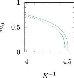
Figure 2: Magnetisation curve near the critical point as obtained in the LPA (symbols) and the fitting curve (55) to the exact MC simulations with the parameters from [27] (solid line).

The simulated temperature range was restricted by 10% distance from $T_{c}$ for the following reasons. First, the correlation length at the lowest temperature was already smaller than the lattice constant (0.8 l.u.) which already is far from the critical region which was of the main interest in the present study. Second, at the lowering temperature the numerical integration considerably slowed down so that convergence to the self-consistent solution by iterations was difficult to achieve. It is not excluded, however, that the LPA in the layer-cake renormalization scheme could describe the low-temperature magnetisation in an asymptotically exact way. As $T\to 0$ $r$ grows very fast so $G({\bf k})$ flattens and the SSA should be adequate. The SSA does reproduce correctly the leading asymptotic correction to the saturated magnetisation $m_{0}=1$ and the LPA may follow the suite, as was discussed in section 4.2. However, this can hardly be verified in numerical calculations because at low temperatures $r$ grows by the Arrhenius law $r\propto e^{AK}$ with $A=O(10)$ so the integration range shrinks as $1/r\sim e^{-AK}$ but at the same time the second derivative $u_{xx}^{0}$ in (58) grows as $r^{2}$ which poses serious computational problems. By all evidence the possibility can be reliably verified only analytically.

7 Discussion

The RG equation in the LPA derived in the present paper has made possible calculation of non-universal quantities in several $n$-vector spin models in good agreement with the known values obtained within reliable techniques such as the high-temperature expansions and the Monte Carlo simulations [16, 27].

The equation, however, has several drawbacks that need be remedied. One deficiency is that it does not reproduce correctly the critical exponents. This, however, may be considered as a minor problem because the exponents are meaningful only asymptotically when the system tends to the criticality. But in this limit the renormalized Hamiltonian simplifies and acquires a universal form [5]. Thus, the layer-cake renormalization can be stopped at sufficiently large value of $t$ and the remaining RG flow accomplished with more rigorous and accurate perturbative techniques. The necessary Feynman diagrams with $\tilde{G}$ (29) can be reduced to the known expressions by separating $\tilde{G}$ into $G$ and $g$. The advantage of this approach is that the necessary parameters of the Hamiltonian [29, 30] will be known to a good accuracy from the LPA solution at $t$.

But the pure LPA approach can be sufficient when the system is not too close to the critical point where the knowledge of accurate values of the exponents is not crucial. For example, from the expression for magnetisation (55) it can be found that already 2% below $T_{c}$ the error due to the deviation of the LPA $\beta=\nu/2$ from the exact value introduces the error in $m$ comparable to the error due to neglect of the correction terms which values depend on non-universal amplitudes $a_{1-2}$. In this situation magnetisation curve calculated in the LPA may be more useful from experimental standpoint than the accurate values of $\beta$ and $\theta_{w}$ provided by the perturbative RG theory.

Much more serious problem is that in the absence of small parameters the closed-form approximations to the exact non-perturbative RG equations are not easy to justify and improve [8] so the good results obtained in several models does not guarantee that they can be trusted in the cases when the correct answers obtained within reliable techniques are unavailable. The LPA is often substantiated by the derivative expansion of the Hamiltonian which in the Fourier space corresponds to expansion in powers of the momenta [8, 24]. However, this argument is valid only in the critical region where the momenta are small. But if an accurate account of irrelevant variables is needed one has to deal with the momenta in the whole BZ where the components of ${\bf k}$ at the boundary reach the values as large as $\pi$ inverse lattice units which obviously is not a suitable expansion parameter.

However, as was pointed out in the Introduction, in lattice systems the short-range fluctuations can be efficiently treated within the cluster approach which may be viewed as a systematic non-perturbative technique but with poor convergence in the critical region. Still, it can be used to initialize renormalization by means of the LPA. Schematically this can be done as follows. First one assumes that $g$ in (29) is not a constant but a function of ${\bf k}$ such that it can be represented as a finite sum of the lattice Fourier terms

$$g({\bf k})=\sum_{|l|\leq L^{c}}g_{l}e^{\mathrm{i}l\cdot{\bf k}}$$ (56)

where $L_{c}$ is a cut-off distance. In the real space the matrix elements ${g}_{ij}$ will vanish beyond the cluster of radius $L_{c}$: $g_{ij}|_{|i-j|>L_{c}}=0$. Now if the system is far from criticality the matrix elements of the self-consistent propagator $G$ exponentially attenuate at large separations (30) [9] and may be neglected for $|i-j|>L_{c}$ when $L_{c}/\xi$ is sufficiently large for the required accuracy. In such a case by choosing $g_{l}\simeq G_{i-j=l}$ in (56) one may neglect $\tilde{G}$ in (29) so the partition function can be calculated within the cluster generalization of the SSA with the use of the clusters of radius $\simeq L_{c}$ (see [3, 4]).

The method just described, however, breaks down in the critical region which is easily seen at the critical point where $G$ is singular at ${\bf k}=0$. Because no finite Fourier sum (56) can reproduce the singularity, $\tilde{G}$ in (29) will be also singular and so not negligible. Still, one can choose $g_{l}$ in (56) in such a way that $g({\bf k})$ satisfactorily approximates $G({\bf k})$ throughout the BZ with the exception of a region surrounding ${\bf k}=0$ with $|{\bf k}|<k_{c}$ where the cut-off $k_{c}\sim 1/L_{c}$. Now the contributions due to $g$ can be calculated within the cluster method while the remaining singular part $\tilde{G}$ for $|{\bf k}|<k_{c}$ accounted for within the LPA with the initial local potential taken from the cluster calculation with the momenta at the vertices set to zero. Within this approach the low-${\bf k}$ region will shrink with growing cluster radius $L_{c}$ which would validate the gradient expansion thus justifying the LPA. Besides, diminishing $k_{c}$ means smaller renormalized interactions which farther validates LPA which is known to be exact to the first order in the interactions [18]. Finally, as $L_{c}$ grows the relative contribution of the singular part into the free energy will diminish which will reduce the errors introduced by the LPA. Thus, with the use of this hybrid cluster/LPA approach the results obtained can be validated without resort to the high-temperature expansions or MC simulations. The feasibility of the approach is supported by the fact that in the purely cluster approach in some cases good convergence could be seen with the use of small easily manageable clusters [3, 4].

In conclusion it is pertinent to note that besides making the LPA-based approach self-contained, the hybrid cluster/LPA technique would enable dealing with the short-range cluster interactions that appear, e.g., in the ab initio theory of alloys [1, 10]. This opens a possibility of developing an approach which would make possible a realistic description of the first- and the second-order phase transitions in lattice systems.

Appendix A Initial condition

The initial effective interaction at $t_{0}$ (27) for $n=1$ case straightforwardly generalizes to the $n$-vector spin models (6) with the use of the $n$-dimensional diffusion kernel as

$$e^{-u^{(n)}({\bf x},t_{0})}=\frac{1}{(2\pi t_{0})^{n/2}}\int d{\bf x}_{0}\,\exp{\left(-\frac{({\bf x-x}_{0})^{2}}{2t_{0}}\right)}\delta({\bf x}_{0}^{2}-1)$$ (57)

where the effective interaction at $t=0$ is given by (6) [16].

The $n=1$ case is trivial

$$u^{(1)}({\bf x},t_{0})=\frac{x^{2}}{2t_{0}}-\ln\cosh\frac{x}{t_{0}}+\mbox{(f.i.t.)}$$ (58)

where $x=|{\bf x}|$ and (f.i.t.) stands for $x$-independent terms.

For $n>1$ in the $O(n)$ symmetric case the integral in (57) is convenient to calculated in hyperspherical coordinates. Choosing the direction of ${\bf x}$ along the first axis ${\bf x}=(x\cos\theta,0,0,\dots,0)$ one gets [31]

$$e^{-u^{(n)}({\bf x},t_{0})}{\;\propto\;}e^{-\frac{x^{2}}{2t_{0}}}\int_{0}^{\pi}e^{\frac{x}{t_{0}}\cos\theta}\sin^{n-2}\theta\,d\theta.$$ (59)

The cases $n=2$ and $n=3$ are given by

$$u^{(2)}({\bf x},t_{0})=\frac{x^{2}}{2t_{0}}-\ln I_{0}\left(\frac{x}{t_{0}}\right)+\mbox{(f.i.t.)}$$

$$u^{(3)}({\bf x},t_{0})=\frac{x^{2}}{2t_{0}}-\ln\left(\frac{t_{0}}{x}\sinh\frac{x}{t_{0}}\right)+\mbox{(f.i.t.)}.$$ (60)

where $I_{0}$ is the modified Bessel function of the first kind.

Explicit expressions for $n>3$ will not be considered in the present paper so we only note that at large $n>8$ a three-term recurrence relation for integrals in (59) can be established so additionally only $n=4-8$ integrals will need to be calculated explicitly in the large-$n$ case.

Appendix B Transformed RG equation

In our case the Legendre transform suggested in [24] (see also [14]) should be slightly modified as

$$y_{\sigma}({\bf x},t)=x_{\sigma}-(t-c)u_{x_{\sigma}}({\bf x},t)$$ (61)

$$v({\bf y},t)=u({\bf x},t)-\frac{1}{2}(t-c)\sum_{\sigma}u_{x_{\sigma}}^{2}({\bf x},t)$$ (62)

where $\sigma=1,\dots,n$ and $c$ is an arbitrary constant. Here the independent variables are ${\bf x}$ and $t$ and the effective interaction is $u$; our aim is to use these relations to re-write (32) in terms of ${\bf y}$ and $t$ for function $v$. To this end we first differentiate Eqs. (61) and (62) with respect to $x_{\sigma^{\prime}}$:

$$\frac{\partial y_{\sigma}}{\partial x_{\sigma^{\prime}}}=\delta_{\sigma\sigma^{\prime}}-(t-c)u_{x_{\sigma}x_{\sigma^{\prime}}}$$ (63)

$$v_{y_{\sigma}}\frac{\partial y_{\sigma}}{\partial x_{\sigma^{\prime}}}=u_{x_{\sigma^{\prime}}}-(t-c)u_{x_{\sigma}}u_{x_{\sigma}x_{\sigma^{\prime}}}.$$ (64)

(we remind the summation over repeated indices convention). Substituting (63) into (64) one gets after some rearrangement a linear system

$$[\delta_{\sigma{\sigma^{\prime}}}-(t-c)u_{x_{\sigma}x_{\sigma^{\prime}}}](v_{y_{\sigma^{\prime}}}-u_{x_{\sigma^{\prime}}})=0.$$ (65)

Because the matrix in this equation in general is not singular it follows that for all $\sigma=1,\cdots,n$

$$v_{y_{\sigma}}=u_{x_{\sigma}}.$$ (66)

Differentiation of this with respect to $x_{\sigma^{\prime}}$ and using (63) gives

$$[\delta_{\sigma\kappa}+(t-c)v_{y_{\sigma}y_{\kappa}}]u_{x_{\kappa}x_{\sigma^{\prime}}}=v_{y_{\sigma}y_{\sigma^{\prime}}}.$$ (67)

As is seen, for fixed $\sigma^{\prime}$ one gets a linear system of size $n$ for expressing $n$ derivatives $u_{x_{\sigma}x_{\sigma^{\prime}}}$ in terms of $v_{y_{\kappa}y_{\kappa^{\prime}}}$.

Finally, differentiating Eqs. (61) and (62) by $t$ and using Eq. (66) one gets (note the difference with equation (15) in [24] where the second term on the l.h.s. is absent)

$$u_{t}+\frac{1}{2}\sum_{\sigma}u_{x_{\sigma}}^{2}=v_{t}$$ (68)

so that (32) can be written as

$$v_{t}=\frac{1}{2}p(t)u_{x_{\sigma}x_{\sigma}}=\frac{1}{2}p(t)\nabla_{\bf x}^{2}u$$ (69)

where the r.h.s. should be expressed in terms of $v_{y_{\sigma}y_{\sigma^{\prime}}}$ with the use of (67). Because (67) depends only on the second order derivatives the annoying negative quadratic terms disappears from (69).

B.1 Fully $O(n)$ symmetric case

In the case of full rotational symmetry (67) can be solved explicitly as follows. Assuming

$$v({\bf y},t)=w(q,t)\mbox{\ where\ }q={\bf y}^{2}/2$$ (70)

one finds

$$v_{y_{\sigma^{\prime}}y_{\sigma}}=\delta_{\sigma^{\prime}\sigma}w_{q}+y_{\sigma^{\prime}}y_{\sigma}w_{qq}.$$ (71)

Now denoting the matrix in (67) as $\hat{M}$ with the use of (71) one gets

$$M_{\sigma\kappa}=\delta_{\sigma\kappa}+(t-c)v_{y_{\sigma}y_{\kappa}}=[1+(t-c)w_{q}]\left[\delta_{\sigma\kappa}+y_{\sigma}y_{\kappa}\frac{(t-c)w_{qq}}{1+(t-c)w_{q}}\right]$$ (72)

Substituting this in (67) and solving for $u_{x_{\sigma}x_{\sigma^{\prime}}}$ one arrives at the expressions that eliminates $u$ and ${\bf x}$ on the r.h.s. of (69) as

$$\nabla^{2}_{\bf x}u=\frac{(n-1)w_{q}}{1+(t-c)w_{q}}+\frac{w_{q}+2qw_{qq}}{1+(t-c)(w_{q}+2qw_{qq})}.$$ (73)

In the case $n=1$ the introduction of $q$ may be superfluous because with $v_{yy}=w_{q}+2qw_{qq}$ the equation simplifies [24].

References

- [1] Ducastelle F 1991 Order and Phase Stability in Alloys (Amsterdam: North-Holland)
- [2] Maier T, Jarrell M, Pruschke T and Hettler M H 2005 Rev. Mod. Phys. 77 1027–1080
- [3] Tokar V I 1997 Comput. Mater. Sci. 8 8–15
- [4] Tan T L and Johnson D D 2011 Phys. Rev. B 83 144427
- [5] Wilson K G and Kogut J 1974 Phys. Rep. 12 75–199
- [6] Le Guillou J C and Zinn-Justin J 1980 Phys. Rev. B 21 3976–3998
- [7] Pelissetto A and Vicari E 2002 Phys. Rep. 368 549–727
- [8] Berges J, Tetradis N and Wetterich C 2002 Phys. Rep. 363 223 – 386
- [9] Tokar V I 1985 Phys. Lett. A 110 453–456
- [10] Blum V and Zunger A 2004 Phys. Rev. B 70 055108
- [11] Tokar V I 2016 Hybrid cluster+RG approach to the theory of phase transitions in strongly coupled Landau-Ginzburg-Wilson model arXiv:1606.06987
- [12] Wegner F J and Houghton A 1973 Phys. Rev. A 8 401–412
- [13] Nicoll J F, Chang T S and Stanley H E 1976 Phys. Rev. A 13 1251–1264
- [14] Bervillier C 2013 Nucl. Phys. B 876 587
- [15] Vasiliev A N 1998 Functional Methods in Quantum Field Theory and Statistical Physics (Amsterdam: Gordon and Breach)
- [16] Butera P and Comi M 2000 Phys. Rev. B 62 14837–14843
- [17] Hori S 1962 Nucl. Phys. 30 644–663
- [18] Tokar V I 1984 Phys. Lett. A 104 135–139
- [19] Lieb E and Loss M 2001 Analysis CRM Proceedings & Lecture Notes (Providence, RI: American Mathematical Society)
- [20] Jelitto R J 1969 J. Phys. Chem. Solids 30 609–626
- [21] Monkhorst H J and Pack J D 1976 Phys. Rev. B 13 5188–5192
- [22] Parola A, Pini D and Reatto L 1993 Phys. Rev. E 48 3321–3332
- [23] Caillol J M 2012 Nuclear Physics B 855 854–884
- [24] Morris T 2005 J. High Energy Phys. 0507 027
- [25] Radhakrishnan K and Hindmarsh A C 1993 Description and use of lsode, the livermore solver for ordinary differential equations Tech. Rep. UCRL-ID-113855 LLNL
- [26] Sanchez J M and de Fontaine D 1978 Phys. Rev. B 17 2926–2936
- [27] Talapov A L and Blöte H W J 1996 J. Phys. A 29 5727
- [28] Liu A J and Fisher M E 1989 Physica 156A 35–76
- [29] Bagnuls C and Bervillier C 1985 Phys. Rev. B 32 7209–7231
- [30] Bagnuls C, Bervillier C, Meiron D I and Nickel B G 1987 Phys. Rev. B 35 3585–3607
- [31] Spherical volume element https://en.wikipedia.org/wiki/N-sphere