End-to-end Sleep Staging with Raw Single Channel EEG using Deep Residual ConvNets

Abstract

Humans approximately spend a third of their life sleeping, which makes monitoring sleep an integral part of well-being. In this paper, a 34-layer deep residual ConvNet architecture for end-to-end sleep staging is proposed. The network takes raw single channel electroencephalogram (Fpz-Cz) signal as input and yields hypnogram annotations for each 30s segments as output. Experiments are carried out for two different scoring standards (5 and 6 stage classification) on the expanded PhysioNet Sleep-EDF dataset, which contains multi-source data from hospital and household polysomnography setups. The performance of the proposed network is compared with that of the state-of-the-art algorithms in patient independent validation tasks. The experimental results demonstrate the superiority of the proposed network compared to the best existing method, providing a relative improvement in epoch-wise average accuracy of 6.8% and 6.3% on the household data and multi-source data, respectively. Codes are made publicly available on Github.

I Introduction

Sleep disorders are becoming a global health problem and more prominent in clinical practice as the global population and life expectancy increases. 50-70 million adults have a sleep disorder in the United States according to the American Sleep Association. Sleep problems were marked as “An Emerging Global Epidemic” following a study by the World Health Organization (WHO) conducted with 40,000 adults from developing countries across Africa and Asia [1]. Sleep plays an essential role in our health and well-being. It affects the regulation of glucose metabolism and loss of sleep could develop a resistance towards insulin, which may result in Type 2 diabetes [2]. In older adults, sleep disorders could be contributing to neuro-degenerative disorders [3]. Polysomnogram (PSG) is widely used as a diagnostic tool to determine sleep disorders. Polysomnography incorporates the recording and inspection of multiple physiological signals during sleep, like electroencephalogram (EEG), electro-oculogram (EOG) and electrocardiogram (ECG). The physiological variables and body movements help experts determine what stages of sleep the subjects have reached and their duration, depending on standard classification guidelines [4]. Many studies in the past few decades have focused on developing automatic sleep stage classification (ASSC) frameworks. Multi-channel systems incorporating EEG, EOG and EMG [5, 6], single-channel systems with EEG [7] and multi-modal systems with smartphone and wearable sensors [8] have been explored. While state-of-the-art systems mostly employ feature extraction based methods along with machine learning algorithms [9], recent papers have adopted the use of Deep Neural Networks (DNN) in an end-to-end fashion [10]. Digital filtering [11] and Wavelet Transform [12, 13], along with its variants [14], have been common pre-processing steps utilized in previous studies. A number of these methods extract time [11], frequency [14] or time-frequency features from each decomposed band of the signal [15]. These features are hand-engineered depending on the study population and therefore may not generalize well. Moreover, there is no consensus on which features are the most discriminatory for the sleep stage classification task [9]. Deep learning methods are known to automatically learn generalizing features, which have been leveraged in a number of different tasks in the past [16]. Recent deep learning approaches for sleep staging have explored end-to-end systems using 1-dimensional Convolutional Neural Networks (1DCNN), Bi-directional Long Short Term Memory Units [10, 17], and also 2DCNNs with prior spectral decomposition to represent EEG as 2D images [7]. In [18], the EEG signal was first pre-processed with a notch and bandpass filter and followed by two separate CNN and Multi-layer Perceptron (MLP) architectures using time domain and frequency domain signals. Deep complex valued CNNs with C3-A2 EEG signals were employed in [19]. A 12-layer deep 1DCNN architecture for feature extraction was explored in [20], while in [10] a 4-layer deep architecture was deployed. In this paper, we introduce a 34-layer deep 1DCNN residual architecture for end-to-end classification. Residual architectures (ResNet) were proposed to resolve the vanishing gradient problem arising from the training of deeper CNN models [16]. As the number of layers used in our model is significantly higher compared to previous studies on sleep staging, we utilize the ResNet architecture for our end-to-end system and compare its performance with state-of-the-art algorithms.

II Dataset

A number of sleep health studies have been compiled into datasets that are used in quantitative experiments, i.e. the Sleep Heart Health Study (SHHS) [20], Montreal Archive of Sleep Studies (MASS) [10] and the Physionet Sleep-EDF Database [21]. We use the Physionet Sleep-EDF Expanded Database in our experiments for its data volume and commonality in existing literature [9]. The database contains a total number of 61 polysomnography recordings from 42 subjects, sampled at 100 Hz. 30s data epochs from each recording were scored by sleep experts into one of the eight classes: AWA (Awake), S1-S4 (intermediate stages), REM (Rapid Eye Movement), MVT (Movement Time) and ’Unscored’ [4]. The MVT and unscored data epochs have been removed prior to our experiments since they don’t correspond to any stages of sleep. We have also fused the S3 and S4 stages for 5-stage classification according to AASM [22]. The PhysioNet Sleep-EDF Expanded Database is assembled from two different studies. The first 39 recordings are from the Sleep Cassette (SC) subset, which was collected from in-home sessions to study the effect of aging on health [23]. This portion of the dataset includes sleep data from 20 healthy subjects without any sleep-related medication. Each patient contributed two different recordings from two nights, except for patient number 13. The latter 22 data samples are from Sleep Telemetry (ST) recording subset. It was collected during a hospital study on the effects of Temazepam on sleep. The data was acquired from 22 subjects for two different nights. Our experiments incorporate recordings from the nights without medication. The distribution of samples from various classes are shown in Table I.

TABLE I: Epochs in each class for different subsets

Subset	Subjects	S1	S2	S3	S4	REM	W	Total
Sleep Cassette	20	2804	17799	3370	2333	7717	71887	105910
Sleep Telemetry	22	2044	9493	1705	1440	4131	2285	21098
Sleep-EDF Total	42	4848	27292	5075	3773	11848	74172	127008
RS-task - Train	30	3499	18824	3339	2462	7857	46862	82843
RS-task - Test	12	1349	8468	1736	1311	3991	27310	44165

III Methodology

III-A Experimental Setup

We design our experiments to address the robustness of deep learning models towards patient independent classification tasks. We have devised two test cases; the first is a multi-source task where a patient independent $71\%-29\%$ random split is performed on data from both SC and ST, from here on referred to as Random Split task (RS-task). There are $42$ recordings ($25$ from $13$ SC subjects & $17$ from $17$ ST subjects) in the training set and $19$ recordings ($14$ from $7$ SC subjects & $5$ from $5$ ST subjects) in the test set of the RS-task. The second case is when we train and test with the Sleep Cassette subset of the dataset with a $70\%-30\%$ random patient independent split, from here on referred to as Sleep Cassette task (SC-task). This task has $27$ recordings from $14$ SC subjects in the training set and $12$ recordings from $6$ SC subjects in the test set. We perform each of these experiments with the FPz-Cz EEG channel data. The specific recording IDs and codes for each test case is available on Github . Table I contains the number of subjects and epochs from each class utilized in each of our experiments.

TABLE II: Comparison of Proposed Method with Accuracy reported on Sleep-EDF Database (Sleep Cassette only)

Approach	No. of Epochs	Split	Method	5-Stage Acc	6-Stage Acc
K. Aboalayon 2016 [11]	23806 Fpz-Cz 10s	80%-20% Not independent	IIR-MMD-DT	95.5%	93.1%
N. Liu 2017 [12]	60647 Fpz-Cz 30s	90%-10% Not independent	DWT-CNN-MLP	-	90.1%
M. Sharma 2018 [13]	85900 Single EEG 30s	10 fold CV Not independent	Wavelet-SVM	91.7%	91.5%
A. Vilamala 2017 [7]	Not Specified	15-4 Independent	Spectral 2D-VGG16	86.0%	-
A. Supratak 2017 [10]	41950 Fpz-Cz 30s	20 patients LOO-CV	CNN-BLSTM	82.0%	-
H. Phan 2018 [17]	46236 Fpz-Cz 30s	20 patients LOO-CV	BLSTM-SVM	82.5%	-
D. Jiang 2019 [15]	54728 Fpz-Cz 30s	20 patients LOO-CV	Multi.Decomp.-RF-HMM	93.0%	-
Proposed Method	127008 Fpz-Cz 30s	70%-30% Independent	Residual CNN	91.4%	90.1%

TABLE III: Performance comparison with Abolayon et al. for $6$-stage classification

Method	Exp. Task	S1 Sens.	Avg Sens.	Avg Spec.	Epoch-Wise Acc	Patient-Wise Acc
IIR-MMD-DT [11]	RS-task	15.6	58.2	95.6	83.8	80.3
IIR-MMD-DT [11]	SC-task	26.4	61.9	94.8	84.3	84.3
Proposed Method	RS-task	43.8	66.5	97.9	88.8	85.5
Proposed Method	SC-task	43.3	67.9	97.0	90.1	90.0

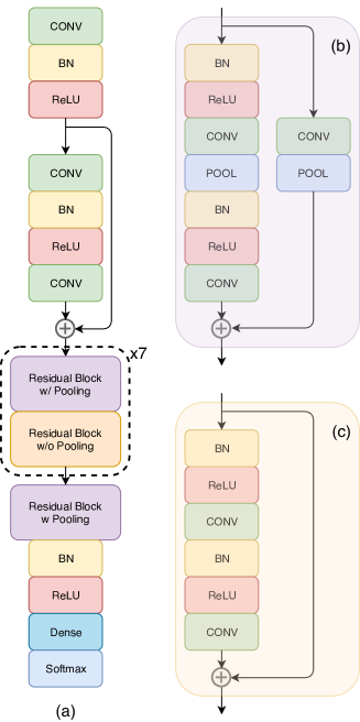
Figure 1: The proposed residual architecture for $6$ class classification of sleep. (a) High-level overview of architecture with residual blocks. (b) Residual block with pooling layers both in the body and skip connection. (c) Residual block architecture without pooling layer.

III-B Proposed Method

Residual architectures have previously been employed for both image classification tasks [24] and biomedical signal processing tasks [25]. They were introduced to make optimization and convergence of very deep neural networks plausible. Training deeper neural networks poses challenges related to saturation and degradation of training accuracy with the increase of layers. Skip-connections in the residual blocks allow deeper CNN layers to approximate an identity operation instead of performing redundant transformations, by only passing the input tensor to the next block. We, therefore, employ skip-connections in our model for sequence-to-sequence sleep staging of each $30s$ EEG data epochs. Our proposed architecture has $34$ 1DCNN layers with the number of kernels in each CNN layer increasing with depth. Our model takes $30s$ unprocessed EEG time-domain signals as input and outputs hypnogram predictions for each instance. Fig. 1 portrays the high-level network architecture. The residual blocks with skip-connections follow a pre-activation design [24] that performs addition operation between the input tensor and the transformed output prior to activation (Fig. 1-c). This allows gradients to flow to shallower layers without aberration. Each CNN layer has a kernel size of $16$ and $64k$ filters where $k\in\{{1,2,3,4}$} increases by $1$ after every $8$ convolutional layers. Each pooling layer performs a max-pooling operation, sub-sampling the incoming data by $2$. The residual blocks with pooling have an extra CNN layer in the shortcut with a kernel size of $1$ and an equal number of filters as the second CNN layer in the corresponding block (Fig. 1-b). It performs a linear combination operation to equalize the depth of the tensors before addition. Activations were dropped-out with a post-activation probability of $0.5$. The network was trained using Adam optimizer with a maximum learning rate of $0.001$ and we divide the learning rate by $10$ after every $10$ training epochs. Cross-entropy loss is weighted according to the dominance of classes in the training population to tackle class imbalance. During training, rolling shifts were performed to augment the training data for improved generalization.

IV Results

We compare the accuracy metric obtained by our proposed method on the SC-task with that reported on recent papers in Table II. The evaluation methods used in literature can be divided into two types. The first is example splitting, where data epochs from the same patient are allowed to be in both the train and test sets; therefore the splits are not patient independent [11, 12, 13]. The other way is to perform patient splitting where patients are split between training and testing to ensure a patient independent test set [7, 10, 17]. Patient splitting can be performed at random [7] or in a leave-one-out cross-validation (LOO-CV) scheme where data from only one patient is used for evaluation [15]. The number of epochs used in the experiments also require consideration. The performance achieved by our proposed method in the SC-task is comparable with the accuracy acquired by state-of-the-art methods on the SC subset of the Physionet Sleep-EDF database, surpassing most except for [15] in patient independent tasks. For a fair comparison between patient independent and not independent splitting, we implement the method proposed by Aboalayon et al. [11], which obtained the best accuracy reported for this problem. In our implementation, we used a Balanced Bagging ensemble of $71$ Decision Trees to compensate for class imbalance. Table III contains comparison of its acquired metrics with our proposed model. Our model exhibits a relative improvement of $6.8\%$ in epoch-wise accuracy on the SC-task and $6.25\%$ on the RS-task. We also evaluate how well our model is performing for individual patients; our model exhibits $6.76\%$ relative increase in patient-wise accuracy on the SC-task and $6.45\%$ increase on the RS-task.

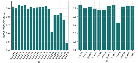
Figure 2: Epoch-wise accuracy for different test set recordings in each task: (a) Random-split task (RS-task) (b) Sleep Cassette task (SC-task).

V Discussion

V-A Number of Epochs and Split

The Sleep-EDF database, though widely employed in quantitative experiments, lacks a standard test bench for fair comparison between different ASSC frameworks. Evaluation metrics are susceptible to changes in class distributions, number of epochs used in the evaluation task and also the epoch selection scheme [20]. We can see a $8.8\%$ reduction in the accuracy of [11] in the $6$-stage SC-task compared to the paper reported metric, which can be due to an increased number of data epochs and patient independent splitting during evaluation. Our SC-task uses data from multiple patients (Fig 2) during test, which is more challenging compared to LOO-CV. This explains the accuracy difference between Jiang et al. [15] and our proposed method (Table II).

V-B Difference between SC & ST subsets

From Fig. 2-a we observe that our model exhibits a drop in accuracy for recordings which are from the ST subset compared to the SC subset. No such trend is visible when the model is trained and evaluated on the SC subset (Fig 2-b). This can be attributed to the presence of data from two different sources in the RS-task which was also discussed in [20]. To explore whether the SC and ST subsets in the Sleep-EDF database exhibit heterogeneous properties or not, we perform one-way ANOVA on two time-domain features (MMD & EnergySis [11]) and two spectral features (Spectral Rolloff & Spectral Spread) extracted from $5$ frequency bands ($\delta,\theta,\alpha,\beta,\gamma$) of the Fpz-Cz channel. Except for the $\gamma$-band EnergySis feature (Fig. 3-a), all of the features exhibit a significant difference in the distribution with a $p\ll 0.001$. Fig 3-b shows significant difference between the density functions of $\gamma$-band Spectral Rolloff between SC and ST. This strengthens our argument regarding heterogeneity between the subsets & explains the accuracy difference between RS-task & SC-task.

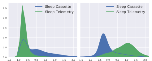
Figure 3: Kernel Density Plots of two different features for Sleep Cassette and Sleep Telemetry subsets a) Scaled $\gamma$-band EnergySis feature b) Scaled $\gamma$-band Spectral Rolloff feature.

VI Conclusion

In this paper, we have proposed a residual architecture based ASSC framework. Our evaluation task comprised of an increased number of data epochs and subjects from multiple sources, compared to previously reported works. Experimental results showed that our model is robust towards noise perturbations which demonstrates relative improvement in epoch-wise average accuracy of $6.8\%$ on the SC-task and $6.3\%$ on the RS-task compared to Aboalayon et al. [11].

Appendix

TABLE IV: Confusion Matrix of our proposed method for 5 Class Classification on SC-task

	S1	S2	S3	REM	AWA
S1	44.23	16.27	0.66	32.55	6.3
S2	4.48	79.72	5.33	4.12	6.35
S3	0.11	21.25	76.58	0	2.06
REM	7.05	8.53	0	75.97	8.45
AWA	2.44	0.15	0.03	1	96.38

TABLE V: Implementation Details of Proposed Architecture

Layer Name	Layer Type	Width	Channels	Params	Input Layer Names
input_1	InputLayer	3000	1	0
conv1d_1	Conv1D	3000	64	1088	input_1
batch_normalization_1	BatchNorm	3000	64	256	conv1d_1
scale_1	Scale	3000	64	128	batch_normalization_1
activation_1	Activation	3000	64	0	scale_1
conv1d_2	Conv1D	3000	64	65536	activation_1
batch_normalization_2	BatchNorm	3000	64	256	conv1d_2
scale_2	Scale	3000	64	128	batch_normalization_2
activation_2	Activation	3000	64	0	scale_2
dropout_1	Dropout	3000	64	0	activation_2
conv1d_3	Conv1D	3000	64	65536	dropout_1
add_1	Add	3000	64	0	conv1d_3,activation_1
batch_normalization_3	BatchNorm	3000	64	256	add_1
scale_3	Scale	3000	64	128	batch_normalization_3
activation_3	Activation	3000	64	0	scale_3
dropout_2	Dropout	3000	64	0	activation_3
conv1d_4	Conv1D	3000	64	65536	dropout_2
max_pooling1d_1	MaxPooling1D	1500	64	0	conv1d_4
batch_normalization_4	BatchNorm	1500	64	256	max_pooling1d_1
scale_4	Scale	1500	64	128	batch_normalization_4
activation_4	Activation	1500	64	0	scale_4
dropout_3	Dropout	1500	64	0	activation_4
conv1d_6	Conv1D	3000	64	4096	add_1
conv1d_5	Conv1D	1500	64	65536	dropout_3
max_pooling1d_2	MaxPooling1D	1500	64	0	conv1d_6
add_2	Add	1500	64	0	conv1d_5.max_pooling1d_2
batch_normalization_5	BatchNorm	1500	64	256	add_2
scale_5	Scale	1500	64	128	batch_normalization_5
activation_5	Activation	1500	64	0	scale_5
dropout_4	Dropout	1500	64	0	activation_5
conv1d_7	Conv1D	1500	64	65536	dropout_4
batch_normalization_6	BatchNorm	1500	64	256	conv1d_7
scale_6	Scale	1500	64	128	batch_normalization_6
activation_6	Activation	1500	64	0	scale_6
dropout_5	Dropout	1500	64	0	activation_6
conv1d_8	Conv1D	1500	64	65536	dropout_5
add_3	Add	1500	64	0	conv1d_8,add_2
batch_normalization_7	BatchNorm	1500	64	256	add_3
scale_7	Scale	1500	64	128	batch_normalization_7
activation_7	Activation	1500	64	0	scale_7
dropout_6	Dropout	1500	64	0	activation_7
conv1d_9	Conv1D	1500	64	65536	dropout_6
max_pooling1d_3	MaxPooling1D	750	64	0	conv1d_9
batch_normalization_8	BatchNorm	750	64	256	max_pooling1d_3
scale_8	Scale	750	64	128	batch_normalization_8
activation_8	Activation	750	64	0	scale_8
dropout_7	Dropout	750	64	0	activation_8
conv1d_11	Conv1D	1500	128	8192	add_3
conv1d_10	Conv1D	750	128	131072	dropout_7
max_pooling1d_4	MaxPooling1D	750	128	0	conv1d_11
add_4	Add	750	128	0	conv1d_10,max_pooling1d_4
batch_normalization_9	BatchNorm	750	128	512	add_4
scale_9	Scale	750	128	256	batch_normalization_9
activation_9	Activation	750	128	0	scale_9
dropout_8	Dropout	750	128	0	activation_9
conv1d_12	Conv1D	750	128	262144	dropout_8
batch_normalization_10	BatchNo	750	128	512	conv1d_12
scale_10	Scale	750	128	256	batch_normalization_10
activation_10	Activation	750	128	0	scale_10
dropout_9	Dropout	750	128	0	activation_10
conv1d_13	Conv1D	750	128	262144	dropout_9
add_5	Add	750	128	0	conv1d_13,add_4
batch_normalization_11	BatchNo	750	128	512	add_5
scale_11	Scale	750	128	256	batch_normalization_11
activation_11	Activation	750	128	0	scale_11
dropout_10	Dropout	750	128	0	activation_11
conv1d_14	Conv1D	750	128	262144	dropout_10
max_pooling1d_5	MaxPooling1D	375	128	0	conv1d_14
batch_normalization_12	BatchNo	375	128	512	max_pooling1d_5
scale_12	Scale	375	128	256	batch_normalization_12
activation_12	Activation	375	128	0	scale_12
dropout_11	Dropout	375	128	0	activation_12
conv1d_16	Conv1D	750	128	16384	add_5
conv1d_15	Conv1D	375	128	262144	dropout_11
max_pooling1d_6	MaxPooling1D	375	128	0	conv1d_16
add_6	Add	375	128	0	conv1d_15,max_pooling1d_6
batch_normalization_13	BatchNo	375	128	512	add_6
scale_13	Scale	375	128	256	batch_normalization_13
activation_13	Activation	375	128	0	scale_13
dropout_12	Dropout	375	128	0	activation_13
conv1d_17	Conv1D	375	128	262144	dropout_12
batch_normalization_14	BatchNo	375	128	512	conv1d_17
scale_14	Scale	375	128	256	batch_normalization_14
activation_14	Activation	375	128	0	scale_14
dropout_13	Dropout	375	128	0	activation_14
conv1d_18	Conv1D	375	128	262144	dropout_13
add_7	Add	375	128	0	conv1d_18,add_6
batch_normalization_15	BatchNo	375	128	512	add_7
scale_15	Scale	375	128	256	batch_normalization_15
activation_15	Activation	375	128	0	scale_15

TABLE VI: Implementation Details of Proposed Architecture (Continued)

Layer Name	Layer Type	Width	Channels	Params	Input Layer Names
dropout_14	Dropout	375	128	0	activation_15
conv1d_19	Conv1D	375	128	262144	dropout_14
max_pooling1d_7	MaxPooling1D	187	128	0	conv1d_19
batch_normalization_16	BatchNo	187	128	512	max_pooling1d_7
scale_16	Scale	187	128	256	batch_normalization_16
activation_16	Activation	187	128	0	scale_16
dropout_15	Dropout	187	128	0	activation_16
conv1d_21	Conv1D	375	192	24576	add_7
conv1d_20	Conv1D	187	192	393216	dropout_15
max_pooling1d_8	MaxPooling1D	187	192	0	conv1d_21
add_8	Add	187	192	0	conv1d_20,max_pooling1d_8
batch_normalization_17	BatchNo	187	192	768	add_8
scale_17	Scale	187	192	384	batch_normalization_17
activation_17	Activation	187	192	0	scale_17
dropout_16	Dropout	187	192	0	activation_17
conv1d_22	Conv1D	187	192	589824	dropout_16
batch_normalization_18	BatchNo	187	192	768	conv1d_22
scale_18	Scale	187	192	384	batch_normalization_18
activation_18	Activation	187	192	0	scale_18
dropout_17	Dropout	187	192	0	activation_18
conv1d_23	Conv1D	187	192	589824	dropout_17
add_9	Add	187	192	0	conv1d_23,add_8
batch_normalization_19	BatchNo	187	192	768	add_9
scale_19	Scale	187	192	384	batch_normalization_19
activation_19	Activation	187	192	0	scale_19
dropout_18	Dropout	187	192	0	activation_19
conv1d_24	Conv1D	187	192	589824	dropout_18
max_pooling1d_9	MaxPooling1D	93	192	0	conv1d_24
batch_normalization_20	BatchNo	93	192	768	max_pooling1d_9
scale_20	Scale	93	192	384	batch_normalization_20
activation_20	Activation	93	192	0	scale_20
dropout_19	Dropout	93	192	0	activation_20
conv1d_26	Conv1D	187	192	36864	add_9
conv1d_25	Conv1D	93	192	589824	dropout_19
max_pooling1d_10	MaxPooling1D	93	192	0	conv1d_26
add_10	Add	93	192	0	conv1d_25,max_pooling1d_10
batch_normalization_21	BatchNo	93	192	768	add_10
scale_21	Scale	93	192	384	batch_normalization_21
activation_21	Activation	93	192	0	scale_21
dropout_20	Dropout	93	192	0	activation_21
conv1d_27	Conv1D	93	192	589824	dropout_20
batch_normalization_22	BatchNo	93	192	768	conv1d_27
scale_22	Scale	93	192	384	batch_normalization_22
activation_22	Activation	93	192	0	scale_22
dropout_21	Dropout	93	192	0	activation_22
conv1d_28	Conv1D	93	192	589824	dropout_21
add_11	Add	93	192	0	conv1d_28,add_10
batch_normalization_23	BatchNo	93	192	768	add_11
scale_23	Scale	93	192	384	batch_normalization_23
activation_23	Activation	93	192	0	scale_23
dropout_22	Dropout	93	192	0	activation_23
conv1d_29	Conv1D	93	192	589824	dropout_22
max_pooling1d_11	MaxPooling1D	46	192	0	conv1d_29
batch_normalization_24	BatchNo	46	192	768	max_pooling1d_11
scale_24	Scale	46	192	384	batch_normalization_24
activation_24	Activation	46	192	0	scale_24
dropout_23	Dropout	46	192	0	activation_24
conv1d_31	Conv1D	93	256	49152	add_11
conv1d_30	Conv1D	46	256	786432	dropout_23
max_pooling1d_12	MaxPooling1D	46	256	0	conv1d_31
add_12	Add	46	256	0	conv1d_30,max_pooling1d_12
batch_normalization_25	BatchNo	46	256	1024	add_12
scale_25	Scale	46	256	512	batch_normalization_25
activation_25	Activation	46	256	0	scale_25
dropout_24	Dropout	46	256	0	activation_25
conv1d_32	Conv1D	46	256	1048576	dropout_24
batch_normalization_26	BatchNo	46	256	1024	conv1d_32
scale_26	Scale	46	256	512	batch_normalization_26
activation_26	Activation	46	256	0	scale_26
dropout_25	Dropout	46	256	0	activation_26
conv1d_33	Conv1D	46	256	1048576	dropout_25
add_13	Add	46	256	0	conv1d_33,add_12
batch_normalization_27	BatchNo	46	256	1024	add_13
scale_27	Scale	46	256	512	batch_normalization_27
activation_27	Activation	46	256	0	scale_27
dropout_26	Dropout	46	256	0	activation_27
conv1d_34	Conv1D	46	256	1048576	dropout_26
max_pooling1d_13	MaxPooling1D	23	256	0	conv1d_34
batch_normalization_28	BatchNo	23	256	1024	max_pooling1d_13
scale_28	Scale	23	256	512	batch_normalization_28
activation_28	Activation	23	256	0	scale_28
dropout_27	Dropout	23	256	0	activation_28
conv1d_36	Conv1D	46	256	65536	add_13
conv1d_35	Conv1D	23	256	1048576	dropout_27
max_pooling1d_14	MaxPooling1D	23	256	0	conv1d_36
add_14	Add	23	256	0	conv1d_35,max_pooling1d_14
batch_normalization_29	BatchNo	23	256	1024	add_14
scale_29	Scale	23	256	512	batch_normalization_29
activation_29	Activation	23	256	0	scale_29
dropout_28	Dropout	23	256	0	activation_29
conv1d_37	Conv1D	23	256	1048576	dropout_28
batch_normalization_30	BatchNo	23	256	1024	conv1d_37
scale_30	Scale	23	256	512	batch_normalization_30
activation_30	Activation	23	256	0	scale_30
dropout_29	Dropout	23	256	0	activation_30
conv1d_38	Conv1D	23	256	1048576	dropout_29
add_15	Add	23	256	0	conv1d_38,add_14
batch_normalization_31	BatchNo	23	256	1024	add_15
scale_31	Scale	23	256	512	batch_normalization_31
activation_31	Activation	23	256	0	scale_31
dropout_30	Dropout	23	256	0	activation_31
conv1d_39	Conv1D	23	256	1048576	dropout_30
max_pooling1d_15	MaxPooling1D	11	256	0	conv1d_39
batch_normalization_32	BatchNo	11	256	1024	max_pooling1d_15
scale_32	Scale	11	256	512	batch_normalization_32
activation_32	Activation	11	256	0	scale_32
dropout_31	Dropout	11	256	0	activation_32
conv1d_41	Conv1D	23	512	131072	add_15
conv1d_40	Conv1D	11	512	2097152	dropout_31
max_pooling1d_16	MaxPooling1D	11	512	0	conv1d_41
add_16	Add	11	512	0	conv1d_40,max_pooling1d_16
batch_normalization_33	BatchNo	11	512	2048	add_16
scale_33	Scale	11	512	1024	batch_normalization_33
activation_33	Activation	11	512	0	scale_33
flatten_1	Flatten	5632	0	0	activation_33
dense_1	Dense	5	0	28165	flatten_1

References

- [1] S. Stranges, W. Tigbe, F. X. Gómez-Olivé, M. Thorogood, and N.-B. Kandala, “Sleep problems: an emerging global epidemic? Findings from the indepth WHO-SAGE study among more than 40,000 older adults from 8 countries across Africa and Asia,” Sleep, vol. 35, no. 8, pp. 1173–1181, 2012.
- [2] K. Spiegel, K. Knutson, R. Leproult, E. Tasali, and E. V. Cauter, “Sleep loss: a novel risk factor for insulin resistance and Type 2 diabetes,” J. of App. Physiol., vol. 99, no. 5, pp. 2008–2019, 2005.
- [3] S. L. Naismith, S. J. Lewis, and N. L. Rogers, “Sleep–wake changes and cognition in neurodegenerative disease,” in Prog. Brain Res., 2011, vol. 190, pp. 21–52.
- [4] J. A. Hobson, “A manual of standardized terminology, techniques and scoring system for sleep stages of human subjects,” Electroencephalogr. Clin. Neurophysiol., vol. 26, no. 6, p. 644, 1969.
- [5] L. Cen, Z. L. Yu, Y. Tang, W. Shi, T. Kluge, and W. Ser, “Deep learning method for sleep stage classification,” in Int. Conf. Neural Information Processing, 2017, pp. 796–802.
- [6] J. Virkkala, J. Hasan, A. Värri, S.-L. Himanen, and K. Müller, “Automatic sleep stage classification using two-channel electro-oculography,” J. of neuroscience methods, vol. 166, no. 1, pp. 109–115, 2007.
- [7] A. Vilamala, K. H. Madsen, and L. K. Hansen, “Deep convolutional neural networks for interpretable analysis of eeg sleep stage scoring,” arXiv preprint arXiv:1710.00633, 2017.
- [8] W. Chen, A. Sano, D. L. Martinez, S. Taylor, A. W. McHill, A. J. Phillips, L. Barger, E. B. Klerman, and R. W. Picard, “Multimodal ambulatory sleep detection,” in Proc. IEEE BHI, 2017, p. 465.
- [9] R. Boostani, F. Karimzadeh, and M. Nami, “A comparative review on sleep stage classification methods in patients and healthy individuals,” Computer methods and programs in biomedicine, vol. 140, pp. 77–91, 2017.
- [10] A. Supratak, H. Dong, C. Wu, and Y. Guo, “DeepSleepNet: a model for automatic sleep stage scoring based on raw single-channel EEG,” IEEE Trans. Neural Syst. Rehabil. Eng., vol. 25, no. 11, pp. 1998–2008, 2017.
- [11] K. Aboalayon, M. Faezipour, W. Almuhammadi, and S. Moslehpour, “Sleep stage classification using eeg signal analysis: a comprehensive survey and new investigation,” Entropy, vol. 18, no. 9, p. 272, 2016.
- [12] N. Liu, Z. Lu, B. Xu, and Q. Liao, “Learning a convolutional neural network for sleep stage classification,” in Proc. CISP-BMEI, 2017, pp. 1–6.
- [13] M. Sharma, D. Goyal, P. Achuth, and U. R. Acharya, “An accurate sleep stages classification system using a new class of optimally time-frequency localized three-band wavelet filter bank,” Computers in biology and medicine, vol. 98, pp. 58–75, 2018.
- [14] A. R. Hassan and M. I. H. Bhuiyan, “A decision support system for automatic sleep staging from eeg signals using tunable q-factor wavelet transform and spectral features,” J. Neurosci. Methods, vol. 271, pp. 107 – 118, 2016.
- [15] D. Jiang, Y.-n. Lu, M. Yu, and W. Yuanyuan, “Robust sleep stage classification with single-channel eeg signals using multimodal decomposition and hmm-based refinement,” Expert Syst. Appl., vol. 121, pp. 188–203, 2019.
- [16] K. He, X. Zhang, S. Ren, and J. Sun, “Delving deep into rectifiers: Surpassing human-level performance on imagenet classification,” in Proc. IEEE ICCV, 2015, pp. 1026–1034.
- [17] H. Phan, F. Andreotti, N. Cooray, O. Y. Chén, and M. De Vos, “Automatic sleep stage classification using single-channel eeg: Learning sequential features with attention-based recurrent neural networks,” in Proc. IEEE EMBC, 2018, pp. 1452–1455.
- [18] M. Manzano, A. Guillén, I. Rojas, and L. J. Herrera, “Deep learning using eeg data in time and frequency domains for sleep stage classification,” in Int. Work-Conference on Artificial Neural Networks, 2017, pp. 132–141.
- [19] J. Zhang and Y. Wu, “Automatic sleep stage classification of single-channel eeg by using complex-valued convolutional neural network,” Biomed. Tech. (Berl), vol. 63, no. 2, pp. 177–190, 2018.
- [20] A. Sors, S. Bonnet, S. Mirek, L. Vercueil, and J.-F. Payen, “A convolutional neural network for sleep stage scoring from raw single-channel eeg,” Biomedical Signal Processing and Control, vol. 42, pp. 107–114, 2018.
- [21] A. L. Goldberger, L. A. Amaral, L. Glass, J. M. Hausdorff, P. Ch, R. G. Mark, J. E. Mietus, G. B. Moody, C.-K. Peng, and H. E. Stanley, “Physiobank, physiotoolkit, and physionet,” Circulation, vol. 101, no. 23, pp. e215–e220, 2000.
- [22] R. B. Berry, R. Brooks, C. E. Gamaldo, S. M. Harding, C. Marcus, and B. Vaughn, “The AASM manual for the scoring of sleep and associated events,” Rules, Terminology and Technical Specifications, Darien, Illinois, AASM, 2012.
- [23] M. Mourtazaev, B. Kemp, A. Zwinderman, and H. Kamphuisen, “Age and gender affect different characteristics of slow waves in the sleep eeg,” Sleep, vol. 18, no. 7, pp. 557–564, 1995.
- [24] K. He, X. Zhang, S. Ren, and J. Sun, “Identity mappings in deep residual networks,” in Proc. ECCV, 2016, pp. 630–645.
- [25] P. Rajpurkar, A. Y. Hannun, M. Haghpanahi, C. Bourn, and A. Y. Ng, “Cardiologist-level arrhythmia detection with convolutional neural networks,” arXiv preprint arXiv:1707.01836, 2017.