A discrete-time $GI^{X}/Geo^{Y}/1$ queue with early arrival system

Abstract: A discrete-time batch service queue with batch renewal input and random serving capacity rule under the late arrival delayed access system (LAS-DA), has recently appeared in the literature [2]. In this paper, we consider the same model under the early arrival system (EAS), since it is more applicable in telecommunication systems where an arriving batch of packets needs to be transmitted in the same slot in which it has arrived. In doing so, we derive the steady-state queue length distributions at various epochs, and show that in limiting case the result gets converted to the continuous-time queue [1]. We discuss few numerical results as well.
Keywords: Batch arrival, Discrete-time queue, Early arrival system, Renewal process

1 Introduction

The continuous-time batch-arrival and batch-service $GI^{X}/M^{Y}/1$ queue has been studied in the past by Economou and Fakinos [6] and Cordeau and Chaudhry [5]. Whereas, the former one gave the probability generating function (pgf) of the system content distribution at points of arrivals, the later one inverted the pgf given in [9] using roots method. Recently, Barbhuiya and Gupta [1] revisited the work in [6] and [5] and proposed a different methodology for the analysis based on difference equation technique, which is analytically as well as computationally tractable.

Observing the limitations of continuous-time queue in modeling digital communications, computer networks, tele-traffic processes and many more, very recently, Barbhuiya and Gupta [2] considered the theoretical and computational aspects of the discrete-time $GI^{X}/Geo^{Y}/1$ queue. They studied the model under the assumption of only late arrival with delayed access system (LAS-DA), according to which, an arrival cannot depart in the same slot in which it has arrived even if the server is idle, as opposed to the early arrival system (EAS). Discrete-time queues with EAS policy are more significant in the modeling of systems where the packets (information) needs to be transmitted in the same slot in which it has arrived, under an urgent situation. With an aim to fill the gap in the literature, this paper studies the $GI^{X}/Geo^{Y}/1$ queue with EAS assumption. The procedure used throughout the analysis runs parallel to that of [2], however, the result differs significantly.

The main contributions of the paper are as follows: (i) we obtain the steady-state queue-length distributions at pre-arrival and arbitrary epochs in a readily presentable form. Consequently, the numerical computation of state probabilities becomes much easier and quite straight forward, (ii) the analysis provides an alternative methodology to solve many special queueing models considered in the past, such as $GI^{X}/Geo/1$ (see [8], [4]), $GI/Geo/1$ (see [3]), (iii) we derive the results of the continuous-time $GI^{X}/M^{Y}/1$ queue from the results of the discrete-time counterpart.

The remaining portion of the paper is organized as follows. In section 2 we provide the model description which is followed by the mathematical analysis and the derivation of queue-length distributions in section 3. In section 4 we discuss few special cases of the model. In section 5 we obtain the results of the continuous-time queue from the discrete-time counterpart and finally present some numerical results in section 6 which is followed by the conclusion.

2 Model description

Though the model has been described in detail in [2], for the sake of completeness, in this section we give a brief overview of it.

Customers arrive in batches of random size $X$ with probability mass function (pmf) $P(X=i)=g_{i}$, $i=1,2,3...,b$, probability generating function (pgf) $G(z)=\sum_{i=1}^{b}g_{i}z^{i},|z|\leq 1$ and the mean batch size $\overline{g}=\sum_{i=1}^{b}ig_{i}$. Here $b\in\mathbb{N}$ is the maximum possible size of the arriving batch. The inter-arrival times of the batches are independent and identically distributed (i.i.d) random variables with common pmf $a_{n}\!=\!P(A\!=\!n)$, $n\!\geq\!1$ (where $A$ is the random variable corresponding to the inter-arrival time), pgf  $A(z)=\sum_{n=1}^{\infty}a_{n}z^{n}$, and mean inter-arrival time $a$ = $\frac{1}{\lambda}=A^{\prime}(1)$. The customers are served in batches by a single server, where the batch-size to be served is a random variable ($Y$) with pmf $P(Y=i)=y_{i}$, $i=1,2,3...$, pgf $Y(z)=\sum_{i=1}^{\infty}y_{i}z^{i},|z|\leq 1$ and the mean batch-size $\overline{y}$. At each service initiation stage the server will serve minimum of {$i$, whole queue} with probability $y_{i}$. The service times $S$ of the batches are independent and geometrically distributed as $P(S=n)=b_{n}=(1-\mu)^{n-1}\mu,~{}0<\mu<1,~{}n\geq 1$, with mean $\frac{1}{\mu}$. The arrival and service processes are independent of each other. The traffic intensity $\rho=\frac{\lambda\overline{g}}{\mu\overline{y}}$ and $\rho<1$ ensures the stability of the system.

3 Analysis of the model

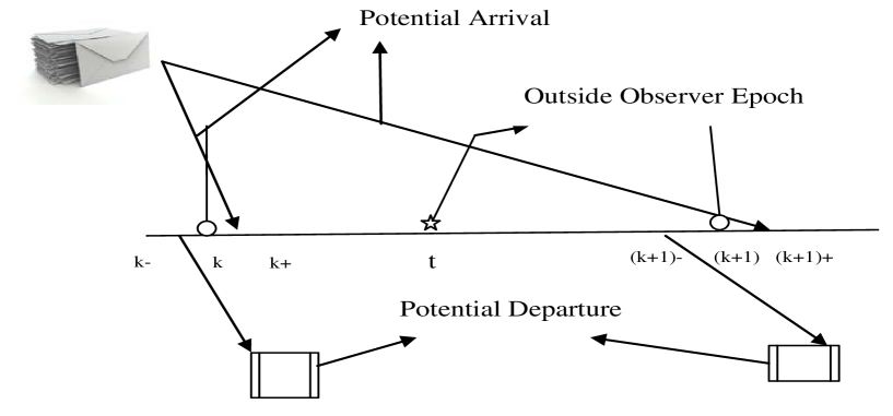
Figure 1: Various epochs for Early Arrival System (EAS)

We consider the early arrival system (EAS) for the present model and accordingly, let the time axis be divided into slots of equal length such that the slot boundaries are marked by $0,1,2,....,k,...$. We assume that the potential batch arrival occurs in $(k,k+$) and the potential batch departure occurs in $(k-,~{}k)$ (see Fig.1). The state of the system just before a potential batch arrival, i.e., at the instant $k$ is described by two random variables $(N_{k},U_{k})$ where $N_{k}$ is the number of customers in the queue and $U_{k}$ is the remaining inter-arrival time of the next batch at the instant $k$. We define the joint distribution of $N_{k}$ and $U_{k}$ as,

$$\widehat{p}_{n}(k,u)=P[N_{k}=n,U_{k}=u],~{}u\geq 0,n\geq 0.$$

Relating the states of the system at two consecutive time epochs $k$ and $k+1$, using the arguments of supplementary variable technique (SVT) by assuming the remaining inter-arrival time of the next batch as the supplementary variable ($u\geq 1$), we obtain the set of governing equations as,

$$\widehat{p}_{0}(u-1,k+1) = \widehat{p}_{0}(u,k)+\mu\sum_{i=1}^{\infty}\widehat{p}_{i}(u,k)\sum_{j=i}^{\infty}y_{j}+a_{u}\mu\sum_{i=0}^{\infty}\widehat{p}_{i}(0,k)\sum_{m=1}^{b}g_{m}\sum_{j=i+m}^{\infty}y_{j},$$ (1)

$$\widehat{p}_{n}(u-1,k+1) = \widehat{p}_{n}(u,k)(1-\mu)+\mu\sum_{i=1}^{\infty}\widehat{p}_{n+i}(u,k)y_{i}+a_{u}(1-\mu)\sum_{i=1}^{n}g_{i}\widehat{p}_{n-i}(0,k)$$ (2)

$$+a_{u}\mu\sum_{i=1}^{\infty}y_{i}\sum_{m=1}^{min\{i+n,b\}}g_{m}\widehat{p}_{n-m+i}(0,k),~{}~{}1\leq n\leq b-1,$$

$$\widehat{p}_{n}(u-1,k+1) = \widehat{p}_{n}(u,k)(1-\mu)+\mu\sum_{i=1}^{\infty}\widehat{p}_{n+i}(u,k)y_{i}+a_{u}(1-\mu)\sum_{i=1}^{b}g_{i}\widehat{p}_{n-i}(0,k)$$ (3)

$$+a_{u}\mu\sum_{i=1}^{\infty}y_{i}\sum_{m=1}^{b}g_{m}\widehat{p}_{n-m+i}(0,k),~{}~{}n\geq b.$$

Further, in steady-state we define $p_{n}(u)=\lim_{k\rightarrow\infty}\widehat{p}_{n}(k,u)$ and thus (1)-(3) reduces to

$$p_{0}(u-1) = p_{0}(u)+\mu\sum_{i=1}^{\infty}p_{i}(u)\sum_{j=i}^{\infty}y_{j}+a_{u}\mu\sum_{i=0}^{\infty}p_{i}(0)\sum_{m=1}^{b}g_{m}\sum_{j=i+m}^{\infty}y_{j}.$$ (4)

$$p_{n}(u-1) = p_{n}(u)(1-\mu)+\mu\sum_{i=1}^{\infty}p_{n+i}(u)y_{i}+a_{u}(1-\mu)\sum_{i=1}^{n}g_{i}p_{n-i}(0)$$ (5)

$$+a_{u}\mu\sum_{i=1}^{\infty}y_{i}\sum_{m=1}^{min\{i+n,b\}}g_{m}p_{n-m+i}(0),~{}~{}~{}1\leq n\leq b-1.$$

$$p_{n}(u-1) = p_{n}(u)(1-\mu)+\mu\sum_{i=1}^{\infty}p_{n+i}(u)y_{i}+a_{u}(1-\mu)\sum_{i=1}^{b}g_{i}p_{n-i}(0)$$ (6)

$$+a_{u}\mu\sum_{i=1}^{\infty}y_{i}\sum_{m=1}^{b}g_{m}p_{n-m+i}(0),~{}~{}~{}n\geq b.$$

In order to obtain the steady-state queue-length distributions we consider the transform $p_{n}^{*}(z)=\sum_{u=0}^{\infty}p_{n}(u)z^{u}$ and $A(z)=\sum_{u=0}^{\infty}a_{u}z^{u}$ such that $a_{0}=0$ and $|z|\leq 1$. This gives $p_{n}^{*}(1)=\sum_{u=0}^{\infty}p_{n}(u)\equiv p_{n}$. Thus, using the transform as defined above, we obtain from (4)-(6) the following

$$(z-1)p_{0}^{*}(z) = \mu\sum_{i=1}^{\infty}p_{i}^{*}(z)\sum_{j=i}^{\infty}y_{j}-p_{0}(0)-\mu\sum_{i=1}^{\infty}p_{i}(0)\sum_{j=i}^{\infty}y_{j}$$ (7)

$$+\mu A(z)\sum_{i=0}^{\infty}p_{i}(0)\sum_{m=1}^{b}g_{m}\sum_{j=i+m}^{\infty}y_{j},$$

$$\left[z-(1-\mu)\right]p_{n}^{*}(z) = \mu\sum_{i=1}^{\infty}y_{i}p_{n+i}^{*}(z)-(1-\mu)p_{n}(0)-\mu\sum_{i=1}^{\infty}y_{i}p_{n+i}(0)$$ (8)

$$+A(z)(1-\mu)\sum_{i=1}^{n}g_{i}p_{n-i}(0)$$

$$+\mu A(z)\sum_{i=1}^{\infty}y_{i}\sum_{m=1}^{min\{i+n,b\}}g_{m}p_{n-m+i}(0),~{}~{}1\leq n\leq b-1.$$

$$\left[z-(1-\mu)\right]p_{n}^{*}(z) = \mu\sum_{i=1}^{\infty}y_{i}p_{n+i}^{*}(z)-(1-\mu)p_{n}(0)-\mu\sum_{i=1}^{\infty}y_{i}p_{n+i}(0)$$ (9)

$$+A(z)(1-\mu)\sum_{i=1}^{b}g_{i}p_{n-i}(0)+\mu A(z)\sum_{i=1}^{\infty}y_{i}\sum_{m=1}^{b}g_{m}p_{n-m+i}(0),n\geq b.$$

Adding (7)-(9), taking limit as $z\rightarrow 1$ and using the normalizing condition $\sum_{n=0}^{\infty}p_{n}=1$ we obtain

$$\sum_{n=0}^{\infty}p_{n}(0)=\frac{1}{a_{1}}=\lambda.$$ (10)

The above result may also be interpreted intuitively as, $p_{n}(0)$ represents the mean number of times the remaining inter-arrival time hits $zero$ per unit time, the sum of which for all $n$ becomes the arrival rate $\lambda$. Let us now define $p_{n}^{-}$ as the probability that the queue-length is $n$ just before the arrival of a batch, i.e., at pre-arrival epoch. As $p_{n}^{-}$ is proportional to $p_{n}(0)$ and $\sum_{n=0}^{\infty}p_{n}^{-}=1$, we have the relation

$$p_{n}^{-}=\frac{p_{n}(0)}{\sum_{k=0}^{\infty}p_{k}(0)}=\frac{p_{n}(0)}{\lambda}.$$ (11)

3.1 Steady-state distribution at pre-arrival and arbitrary epochs

For the sequence of probabilities $\{p_{n}(0)\}_{0}^{\infty}$ and $\{p_{n}^{*}(z)\}_{0}^{\infty}$ we define the right shift operator $D$ as $Dp_{n}(0)=p_{n+1}(0)$ and $Dp_{n}^{*}(z)=p_{n+1}^{*}(z)$ for all $n$. Thus (9) can be rewritten as

$$\left[z-(1-\mu+\mu\sum_{i=1}^{\infty}y_{i}D^{i})\right]p_{n}^{*}(z) = \left[-(1-\mu)D^{b}-\mu\sum_{i=1}^{\infty}y_{i}D^{i+b}+A(z)(1-\mu)\sum_{i=1}^{b}g_{i}D^{b-i}\right.$$ (12)

$$\left.+A(z)\mu\sum_{m=1}^{b}g_{m}\sum_{i=1}^{\infty}y_{i}D^{b+i-m}\right]p_{n-b}(0),~{}~{}n\geq b.$$

Substituting $z=1-\mu+\mu\sum_{i=1}^{\infty}y_{i}D^{i}$ in (12) we get

$$\left[-(1-\mu)D^{b}-\mu\sum_{i=1}^{\infty}y_{i}D^{i+b}+A(1-\mu+\mu\sum_{i=1}^{\infty}y_{i}D^{i})(1-\mu)\sum_{i=1}^{b}g_{i}D^{b-i}\right.$$

$$\left.+A(1-\mu+\mu\sum_{i=1}^{\infty}y_{i}D^{i})\mu\sum_{m=1}^{b}g_{m}\sum_{i=1}^{\infty}y_{i}D^{b+i-m}\right]p_{n}(0) = 0,~{}~{}{n\geq 0},$$ (13)

which is a homogeneous difference equation with constant coefficient with the corresponding characteristic equation (c.e.) as $\left(A(1-\mu+\mu Y(s))\sum_{i=1}^{b}g_{i}s^{b-i}-s^{b}\right)\left(1-\mu+\mu Y(s)\right)=0$. But since

$$A(1-\mu+\mu Y(s))\sum_{i=1}^{b}g_{i}s^{b-i}-s^{b}=0$$ (14)

has exactly $b$ roots inside the unit circle under the stability condition $\rho=\frac{\lambda\overline{g}}{\mu\overline{y}}<1$ (see Barbhuiya and Gupta [2]), hence the c.e. has exactly $b$ roots inside $|s|=1$ denoted by $r_{1},r_{2},...,r_{b}$. Thus the general solution of (13) is given by

$$p_{n}(0) = \sum_{i=1}^{b}c_{i}r_{i}^{n}~{},~{}n\geq 0,$$ (15)

where $c_{1},c_{2},...,c_{b}$ are the arbitrary constants yet to be determined. Substituting the expression of $p_{n}(0)$ from (15) in (12) we obtain

$$\left(z-(1-\mu+\mu\sum_{i=1}^{\infty}y_{i}D^{i})\right)p_{n}^{*}(z) = -(1-\mu)\sum_{j=1}^{b}c_{j}r_{j}^{n}-\mu\sum_{i=1}^{\infty}y_{i}\sum_{j=1}^{b}c_{j}r_{j}^{n+i}$$ (16)

$$+A(z)(1-\mu)\sum_{i=1}^{b}g_{i}\sum_{j=1}^{b}c_{j}r_{j}^{n-i}$$

$$+A(z)\mu\sum_{m=1}^{b}g_{m}\sum_{i=1}^{\infty}y_{i}\sum_{j=1}^{b}c_{j}r_{j}^{n+i-m},~{}~{}{n\geq b}.$$

which is a non-homogeneous difference equation and its general solution is given by

$$p_{n}^{*}(z)=\sum\limits_{j}d_{j}s_{j}^{n}(z)+\sum_{j=1}^{b}c_{j}\left\{\frac{(1-\mu+\mu Y(r_{j}))(A(z)\sum\limits_{i=1}^{b}g_{i}r_{j}^{b-i}-r_{j}^{b})}{z-1+\mu-\mu Y(r_{j})}\right\}r_{j}^{n-b},~{}{n\geq b}.$$ (17)

In (17) the first term in the R.H.S is the solution corresponding to the homogeneous part of (16), the second term is the particular solution, $s_{j}(z)$’s are the roots of $z-1+\mu-\mu Y(s)=0$ for a fixed $z$ and $d_{j}$’s are the corresponding arbitrary constants. Since $\sum_{n=0}^{\infty}p_{n}=1$, so $\sum_{n=b}^{\infty}p_{n}\leq 1$ i.e., $\sum_{n=b}^{\infty}p_{n}^{*}(1)\leq 1$. Setting $z=1$ and summing over $n$ from $b$ to $\infty$ in (17), we have the first term in R.H.S as $\sum\limits_{j}d_{j}(\sum\limits_{n=b}^{\infty}s_{j}^{n}(1))$, where $s_{j}(1)$ are the roots of $Y(s)=1$. These roots lie outside and on the unit circle $|s|=1$ (for proof, see Barbhuiya and Gupta [2]) and hence $\sum_{n=b}^{\infty}s_{j}^{n}(1)$ diverges. Thus to ensure the convergence of (17) we must have $d_{j}=0$ for all $j$ and consequently we get the general solution of (16) as

$$p_{n}^{*}(z)=\sum_{j=1}^{b}c_{j}\left\{\frac{(1-\mu+\mu Y(r_{j}))(A(z)\sum\limits_{i=1}^{b}g_{i}r_{j}^{b-i}-r_{j}^{b})}{z-1+\mu-\mu Y(r_{j})}\right\}r_{j}^{n-b},~{}{n\geq b}.$$ (18)

For $p_{n}^{*}(z)$, $1\leq n\leq b-1$, we seek a similar expression as given in (18). Thus we need to find the conditions under which $p_{n}^{*}(z)$, $1\leq n\leq b-1$ satisfies (8). Substituting the respective expressions in (8) we obtain

$$\sum_{j=1}^{b}c_{j}r_{j}^{n}\left\{(1-\mu)\sum_{i=n+1}^{b}g_{i}r_{j}^{-i}+\mu\sum_{i=1}^{\infty}y_{i}r_{j}^{i}\left(\sum_{m=1}^{b}g_{m}r_{j}^{-m}-\sum_{m=1}^{min(i+n,b)}g_{m}r_{j}^{-m}\right)\right\} = 0,$$

$${1\leq n\leq b-1}.$$ (19)

Putting $n=b-1,~{}b-2,...,1$ in (19) and using the condition that $g_{b}\neq 0$, we obtain the following set of $b-1$ equations:

$$\sum_{j=1}^{b}\frac{c_{j}}{r_{j}}=\sum_{j=1}^{b}\frac{c_{j}}{r_{j}^{2}}=...=\sum_{j=1}^{b}\frac{c_{j}}{r_{j}^{b-2}}=\sum_{j=1}^{b}\frac{c_{j}}{r_{j}^{b-1}}=0.$$ (20)

Also summing over $n$ from $0$ to $\infty$ in (15) and using (10) we obtain

$$\lambda=\sum_{i=1}^{b}\frac{c_{i}}{1-r_{i}}.$$ (21)

Solving the system of $b$ equations (20) and (21), we can obtain the constants $c_{j}$ for $j=1,2,...,b$. This makes the expression of $p_{n}(0)$ ($n\geq 0$) given in (15) completely known. Moreover, $p_{n}^{*}(z)$ is given by

$$p_{n}^{*}(z)=\sum_{j=1}^{b}c_{j}\left\{\frac{(1-\mu+\mu Y(r_{j}))(A(z)\sum\limits_{i=1}^{b}g_{i}r_{j}^{b-i}-r_{j}^{b})}{z-1+\mu-\mu Y(r_{j})}\right\}r_{j}^{n-b},~{}n\geq 1.$$ (22)

Therefore, using (11), (15) and (22) we get the explicit expression of the system content distributions at pre-arrival ($p_{n}^{-}$) and arbitrary ($p_{n}$) epochs as

$$p_{n}^{-} = \frac{1}{\lambda}\sum\limits_{i=1}^{b}c_{i}r_{i}^{n}~{},~{}n\geq 0,$$ (23)

$$p_{n} = p_{n}^{*}(1)=\sum_{j=1}^{b}c_{j}\left\{\frac{(1-\mu+\mu Y(r_{j}))(\sum\limits_{i=1}^{b}g_{i}r_{j}^{b-i}-r_{j}^{b})}{\mu(1-Y(r_{j}))}\right\}r_{j}^{n-b},~{}n\geq 1,$$ (24)

$$p_{0} = 1-\sum_{n=1}^{\infty}p_{n}=1-\sum_{j=1}^{b}c_{j}\left\{\frac{(1-\mu+\mu Y(r_{j}))(\sum\limits_{i=1}^{b}g_{i}r_{j}^{1-i}-r_{j})}{\mu(1-r_{j})(1-Y(r_{j}))}\right\}.$$ (25)

This completes the analysis of $GI^{X}/Geo^{Y}/1$ queue under EAS policy. The results of many special cases of this model can be obtained directly from (23)-(25) as discussed in the forthcoming section. However, we now provide a small example to give an overview of the present analysis to the readers.

Example: Consider a discrete-time $Geo^{X}/Geo^{Y}/1$ queue, i.e., the inter-arrival time follows geometric distribution. Suppose $\lambda=0.2$, $\mu=0.5$ and the mean inter-arrival time is $a=\frac{1}{\lambda}$. Let the arriving batch size distribution is $g_{1}=0.4$, $g_{2}=0.3$ and $g_{3}=0.3$ and service batch size distribution is $y_{1}=0.4$ and $y_{2}=0.6$. This gives $b=3$, $G(z)=0.4z+0.3z^{2}+0.3z^{3}$, $Y(z)=0.4z+0.6z^{2}$, $\overline{g}=1.9$, $\overline{y}=1.6$, $\rho=0.475$ and $A(z)=\frac{\lambda z}{1-(1-\lambda)z}$.

The root equation as deduced from equation (14) is

$$1-A(1-\mu+\mu Y(s))\sum_{i=1}^{3}g_{i}s^{-i} = 0$$

$$\textrm{i.e.,}~{}~{}~{}0.24s^{5}+0.184s^{4}-0.566s^{3}+0.07s^{2}+0.042s+0.03 = 0.$$ (26)

The corresponding roots are $-2.002850$, $-0.183817\pm 0.263763i$, $0.603819$, $1.0$. Clearly, $r_{1}=-0.183817+0.263763i$, $r_{2}=-0.183817-0.263763i$ and $r_{3}=0.603819$ as $|r_{i}|<1$ for $i=1,2,3$. Now the system of three equations deduced from (20) and (21) are

$$\frac{c_{1}}{-0.183817+0.263763i}+\frac{c_{2}}{-0.183817-0.263763i}+\frac{c_{3}}{0.603819} = 0$$

$$\frac{c_{1}}{(-0.183817+0.263763i)^{2}}+\frac{c_{2}}{(-0.183817-0.263763i)^{2}}+\frac{c_{3}}{(0.603819)^{2}} = 0$$

$$\frac{c_{1}}{1.183817-0.263763i}+\frac{c_{2}}{1.183817+0.263763i}+\frac{c_{3}}{0.396181} = 0.2$$

which can be solved to obtain $c_{1}=0.027481-0.000834i$, $c_{2}=0.027481+0.000834i$ and $c_{3}=0.061593$. With the known values of $c_{i}$’s and $r_{i}$’s for $i=1,2,3$, the steady state probabilities at pre-arrival ($p_{n}^{-}$) and arbitrary ($p_{n}$) epochs can be directly evaluated using (23), (24) and (25) as $p_{0}^{-}=p_{0}=0.582779$, $p_{1}^{-}=p_{1}=0.137643$, $p_{2}^{-}=p_{2}=0.101641$, $p_{3}^{-}=p_{3}=0.076705$ and so on. Here both the state probabilities are equal due to Bernoulli arrivals. Furthermore, the average system-content at pre-arrival ($L^{-}$) and arbitrary ($L$) epochs are given by $L^{-}=\sum_{n=1}^{N}np_{n}^{-}=1.133649$ and $L=\sum_{n=1}^{N}np_{n}=1.133649$ for a sufficiently large $N(=500)$. Meanwhile, as the value of $n$ becomes larger (say $n>30$), the ratio $p_{n+1}^{-}/p_{n}^{-}$ tends to $0.603819$ which is $r_{3}$, the unique largest real root inside the unit circle (see Barbhuiya and Gupta [2]).

4 Special Cases

In this section, we discuss some special queueing models whose results can be deduced directly from the analysis done in Section 3.1.

• The model $GI^{X}/Geo^{Y}/1$ reduces to $GI^{X}/Geo/1$ if we consider $y_{1}=1$ and $y_{i}=0$ for $i\geq 2$, i.e., the pgf $Y(s)=s$. Accordingly, the system content distribution at pre-arrival and arbitrary epochs reduces to

  $$p_{n}^{-} = \frac{1}{\lambda}\sum\limits_{i=1}^{b}c_{i}r_{i}^{n}~{},~{}n\geq 0,$$

  $$p_{n} = \sum_{j=1}^{b}c_{j}\left\{\frac{(1-\mu+\mu r_{j})(\sum\limits_{i=1}^{b}g_{i}r_{j}^{b-i}-r_{j}^{b})}{\mu(1-r_{j})}\right\}r_{j}^{n-b},~{}n\geq 1,$$

  $$p_{0} = 1-\sum_{j=1}^{b}c_{j}\left\{\frac{(1-\mu+\mu r_{j})(\sum\limits_{i=1}^{b}g_{i}r_{j}^{1-i}-r_{j})}{\mu(1-r_{j})^{2}}\right\}.$$

  where $r_{j}$’s are the $b$ roots of $A(1-\mu+\mu s)\sum_{i=1}^{b}g_{i}s^{b-i}-s^{b}=0$ inside the unit circle and the constants $c_{j}$, $j=1,2,...b$ can be obtained by solving the system of equations (20) and (21). This model was earlier considered by Chaudhry and Gupta [4] and Vinck and Bruneel [8]. However, the analysis carried out in this paper provides and alternative approach to the solution of the model.

• Similarly, we can obtain the results for $GI/Geo^{Y}/1$ queue by taking $g_{1}=1$ and $g_{i}=0$ for $i\geq 2$, i.e., the pgf $G(s)=s$. The single root inside the unit circle corresponding to (14) is denoted by $r_{1}$ and the constant obtained from (21) is $c_{1}=\lambda(1-r_{1})$. Thus, the distribution at pre-arrival and arbitrary epochs reduces to

  $$p_{n}^{-} = (1-r_{1})r_{1}^{n}~{},~{}n\geq 0,$$

  $$p_{n} = \frac{\lambda(1-r_{1})^{2}(1-\mu+\mu Y(r_{1}))r_{1}^{n-1}}{\mu(1-Y(r_{1}))},~{}n\geq 1,$$

  $$p_{0} = 1-\frac{\lambda(1-r_{1})(1-\mu+\mu Y(r_{1}))}{\mu(1-Y(r_{1}))}.$$

• Along the same line if we consider $g_{1}=1$, $g_{i}=0$ for $i\geq 2$ and $y_{1}=1$, $y_{i}=0$ for $i\geq 2$, then $GI^{X}/Geo^{Y}/1$ queue reduces to the $GI/Geo/1$ queue. Here the pgf’s $G(s)=s$ and $Y(s)=s$, the single root inside the unit circle corresponding to (14) is denoted by $r_{1}$ with the constant obtained as $c_{1}=\lambda(1-r_{1})$. Consequently, the probability distribution obtained at pre-arrival and arbitrary epochs are given by

  $$p_{n}^{-} = (1-r_{1})r_{1}^{n}~{},~{}n\geq 0,$$

  $$p_{n} = \frac{\lambda}{\mu}(1-r_{1})(1-\mu+\mu r_{1})r_{1}^{n-1},~{}n\geq 1,$$

  $$p_{0} = 1-\frac{\lambda}{\mu}(1-\mu+\mu r_{1}).$$

  These results exactly matches with the one obtained by Chaudhry et al. [3].

5 Results of continuous-time $GI^{X}/M^{Y}/1$ queue

In this section we convert the analytical results obtained for the discrete-time queue to the corresponding continuous-time $GI^{X}/M^{Y}/1$ queue. However, the results of discrete-time queues cannot be derived from the continuous time counterpart (see Takagi [7]). So for the continuous time case, we assume the random variable $\widehat{A}$ as the inter-arrival times between two successive batches which are i.i.d with distribution function $\widehat{A}(x)$, Laplace-Stieltjes transform (L.S.T) $A^{*}(s)$ and mean $\frac{1}{\widehat{\lambda}}$, where $\widehat{\lambda}$ is the arrival rate of the batches. The service times $\widehat{S}$ of the batches are exponentially distributed with rate $\widehat{\mu}$. Let the time axis be divided into intervals of equal length $\Delta$, such that $\Delta>0$ and is sufficiently small. Thus we have, $a_{n}=Pr((n-1)\Delta<\widehat{A}\leq n\Delta)$, $n\geq 1$ and $E(A)\Delta=E(\widehat{A})$. One may note that $\widehat{\lambda}\Delta=\lambda$ and $\widehat{\mu}\Delta=\mu$. We now prove that the c.e. (14) reduces to the c.e. corresponding to the continuous-time queue [1].

$$A(1-\mu+\mu Y(s)) \equiv \lim_{\Delta\rightarrow 0}A(1-\widehat{\mu}\Delta+\widehat{\mu}\Delta Y(s))$$

$$= \lim_{\Delta\rightarrow 0}\sum_{n=1}^{\infty}Pr((n-1)\Delta<\widehat{A}\leq n\Delta)[1-\widehat{\mu}\Delta+\widehat{\mu}\Delta Y(s)]^{n}$$

$$= \lim_{\Delta\rightarrow 0}\sum_{n=1}^{\infty}[\widehat{A}(n\Delta)-\widehat{A}((n-1)\Delta)]\left[1-\frac{\widehat{\mu}(1-Y(s))\Delta n}{n}\right]^{n}$$

$$= \int_{0}^{\infty}e^{-\widehat{\mu}(1-Y(s))x}d\widehat{A}(x)$$

$$= A^{*}(\widehat{\mu}(1-Y(s)))$$

Thus, $A^{*}(\widehat{\mu}(1-Y(s)))\sum_{i=1}^{b}g_{i}s^{b-i}-s^{b}=0$ represents the c.e. corresponding to the continuous time queue, which also have exactly $b$ roots ($\widehat{r}_{1}$, $\widehat{r}_{2}$, …, $\widehat{r}_{b}$) inside the unit circle $|s|=1$. Now replacing $r_{j}$’s by $\widehat{r}_{j}$’s, $\lambda$ by $\widehat{\lambda}\Delta$ in (20) and (21) and solving the new system of equations, we obtain the constants in terms of $\Delta$, or to be precise, as linear functions of $\Delta$ i.e., $\widehat{c}_{j}\Delta$ such that $\widehat{c}_{j}$ for $j=1,2,...,b$ are known. Again using $\widehat{\lambda}\Delta=\lambda$, $\widehat{\mu}\Delta=\mu$, $r_{j}=\widehat{r}_{j}$, $c_{j}=\widehat{c}_{j}\Delta$ and taking limit as $\Delta\rightarrow 0$ in (23)-(25) we obtain the pre-arrival and arbitrary epoch probabilities as given in Barbhuiya and Gupta [1].

$$p_{n}^{-} = \frac{1}{\widehat{\lambda}}\sum_{j=1}^{b}\widehat{c}_{j}\widehat{r}_{j}^{n},~{}~{}n\geq 0$$

$$p_{n} = \sum_{j=1}^{b}\widehat{c}_{j}\left\{\frac{G(\widehat{r}_{j}^{-1})-1}{\widehat{\mu}(1-Y(\widehat{r}_{j}))}\right\}\widehat{r}_{j}^{n},~{}~{}n\geq 1$$

$$p_{0} = 1-\sum_{j=1}^{b}\widehat{c}_{j}\left\{\frac{\sum\limits_{i=1}^{b}g_{i}\widehat{r}_{j}^{1-i}-\widehat{r}_{j}}{\widehat{\mu}(1-\widehat{r}_{j})(1-Y(\widehat{r}_{j}))}\right\}.$$

6 Numerical Results

In this section, we present few numerical results in the self explanatory tables in order to demonstrate an overview of the theoretical work done so far. The numerical results are provided correct upto six decimal places. The input parameters taken for deterministic ($D$) inter-arrival time distribution in Table 1 are same as given in Chaudhry and Gupta [4]. It can be observed that the numerical values for $p_{n}^{-}$ and $p_{n}$ exactly matches with that of Chaudhry and Gupta [4], as expected. In addition to that, we have considered arbitrary, geometric ($Geo$) and deterministic ($D$) inter-arrival time distributions, as given in Table 1 and 2 respectively. Whereas, in Table 2 one may observe that the service batch-size distribution is taken as geometric with parameter 0.4, whose pgf is $Y(z)=\frac{0.4z}{1-0.6z}$. A noticeable feature from the distributions taken here is that, the server can comply with infinite support also, and the service batch-size distribution (with infinite support) need not to be truncated to obtain the set of probabilities $p_{n}^{-}$ and $p_{n}$. It is clearly an advantage of our methodology developed here. Moreover an important observation is that, in the limiting case the ratio of the pre-arrival epoch probabilities $\frac{p_{n+1}^{-}}{p_{n}^{-}}$ converges to the largest root in absolute value of the c.e. (14) lying inside the unit circle (for analytical proof, one may refer to Barbhuiya and Gupta [2]). We can thus infer that, the tail probabilities at pre-arrival epoch can be approximated by the root of the c.e. with largest modulus inside the unit circle.

Table 1: System content distribution at pre-arrival ($p_{n}^{-}$) and arbitrary ($p_{n}$) epochs

	$GI\equiv D$			$GI\equiv\textrm{arbitrary}$
	$g_{1}=0.2,~{}g_{5}=0.3,~{}g_{10}=0.5,~{}\bar{g}=6.7$			$g_{2}=0.2,~{}g_{3}=0.3,~{}g_{5}=0.3,~{}g_{8}=0.2,$
	$b=10,~{}Y(z)=z,~{}\mu=0.9,~{}\lambda=0.1,$			$\bar{g}=4.4,~{}b=8,~{}\mu=0.4,~{}\lambda=0.1667,$
	$\rho=0.7444$			$Y(z)=0.3z+0.2z^{3}+0.25z^{4}+0.25z^{6},$
				$\rho=0.539,~{}a_{7}=0.5,~{}a_{10}=0.2,~{}a_{15}=0.3$
$n$	$p_{n}^{-}$	$p_{n}$	$p_{n+1}^{-}/p_{n}^{-}$	$p_{n}^{-}$	$p_{n}$	$p_{n+1}^{-}/p_{n}^{-}$
0	0.578601	0.313415	0.253224	0.878471	0.406746	0.037114
1	0.146516	0.067368	0.742023	0.032604	0.093348	0.804337
2	0.108718	0.075652	0.613434	0.026224	0.130608	0.697163
3	0.066691	0.081029	0.595849	0.018283	0.096706	0.892676
4	0.039738	0.084169	0.599919	0.016321	0.067738	0.649924
5	0.023840	0.068693	0.601121	0.010607	0.090820	0.465432
6	0.014330	0.063502	0.600828	0.004937	0.016528	1.148267
7	0.008610	0.060433	0.600749	0.005669	0.028922	0.711361
8	0.005173	0.058478	0.600771	0.004033	0.049630	0.254162
$\vdots$	$\vdots$	$\vdots$	$\vdots$	$\vdots$	$\vdots$	$\vdots$
124	0.000000	0.000000	0.600774	0.000000	0.000000	0.589450
125	0.000000	0.000000	0.600774	0.000000	0.000000	0.589450
126	0.000000	0.000000	0.600774	0.000000	0.000000	0.589450
127	0.000000	0.000000	0.600774	0.000000	0.000000	0.589450
$\vdots$	$\vdots$	$\vdots$	$\vdots$	$\vdots$	$\vdots$	$\vdots$
sum	1.000000	1.000000		0.999999	0.999999
mean	$L^{-}=1.11$	$L=3.73$		$L^{-}=0.39$	$L=2.27$

Table 2: System-content distribution at pre-arrival ($p_{n}^{-}$) and arbitrary ($p_{n}$) epochs

	$GI\equiv Geo$			$GI\equiv D$
	$g_{2}=0.2,~{}g_{5}=0.25,~{}g_{10}=0.3,~{}g_{12}=0.25,$			$g_{1}=0.3,~{}g_{4}=0.3,~{}g_{6}=0.4,~{}\bar{g}=3.9,~{}b=6,$
	$\bar{g}=7.65,~{}b=12,~{}\mu=0.5,~{}\lambda=0.2,~{}\rho=0.651$			$\mu=0.6,~{}\lambda=0.2,~{}Y(z)=\frac{0.4z}{1-0.6z},~{}\rho=0.52$
	$Y(z)=0.2z^{2}+0.3z^{4}+0.4z^{6}+0.1z^{7},$
$n$	$p_{n}^{-}$	$p_{n}$	$p_{n+1}^{-}/p_{n}^{-}$	$p_{n}^{-}$	$p_{n}$	$p_{n+1}^{-}/p_{n}^{-}$
0	0.359677	0.359677	0.063929	0.730813	0.480000	0.095772
1	0.022994	0.022994	1.608902	0.069991	0.097442	0.855181
2	0.036995	0.036995	0.627629	0.059855	0.077541	0.805875
3	0.023219	0.023219	1.533170	0.048236	0.082722	0.723580
4	0.035599	0.035599	0.935126	0.034902	0.086760	0.645443
5	0.033289	0.033289	1.209728	0.022528	0.060251	0.592548
6	0.040271	0.040271	0.448552	0.013349	0.059059	0.551151
7	0.018064	0.018064	1.868597	0.007357	0.018567	0.660793
8	0.033753	0.033753	0.524978	0.004862	0.013352	0.636454
$\vdots$	$\vdots$	$\vdots$	$\vdots$	$\vdots$	$\vdots$	$\vdots$
124	0.000004	0.000004	0.926546	0.000000	0.000000	0.620481
125	0.000004	0.000004	0.926586	0.000000	0.000000	0.620481
126	0.000004	0.000004	0.926549	0.000000	0.000000	0.620481
127	0.000004	0.000004	0.926583	0.000000	0.000000	0.620481
$\vdots$	$\vdots$	$\vdots$	$\vdots$	$\vdots$	$\vdots$	$\vdots$
sum	1.000000	1.000000		0.999999	1.000000
mean	$L^{-}=9.63$	$L=9.63$		$L^{-}=0.84$	$L=1.99$

7 Conclusion

In this paper, we have studied a discrete time $GI^{X}/Geo^{Y}/1$ queue under early arrival system (EAS). We have used supplementary variable technique and difference equation approach and obtained the steady-state queue-length distribution at pre-arrival and arbitrary epochs in a tractable way. The notable feature of this novel approach is that, it does not require the formation of any complex transition probability matrix, that usually appears in conventional methodologies. We have derived the analytical results of the continuous-time queue from the discrete-time counterpart. Also, we have discussed some numerical results along with some special cases of our model that can be directly derived from the analysis. The results thus obtained may be used in discrete-time systems arising in telecommunications and computer networks where emergency cases needs to be addressed during the transmission of packets.

References

- [1] FP Barbhuiya and UC Gupta. A difference equation approach for analysing a batch service queue with the batch renewal arrival process. Journal of Difference Equations and Applications, pages 1–10, 2019.
- [2] FP Barbhuiya and UC Gupta. Discrete-time queue with batch renewal input and random serving capacity rule: . Queueing Systems, 91(3):347–365, 2019.
- [3] ML Chaudhry, UC Gupta, and James GC Templeton. On the relations among the distributions at different epochs for discrete-time . Operations Research Letters, 18(5):247–255, 1996.
- [4] Mohan L Chaudhry and Umesh Chandra Gupta. Queue-length and waiting-time distributions of discrete-time queueing systems with early and late arrivals. Queueing Systems, 25(1-4):307–324, 1997.
- [5] J Leo Cordeau and Mohan L Chaudhry. A simple and complete solution to the stationary queue-length probabilities of a bulk-arrival bulk-service queue. Infor, 47:283–288, 2009.
- [6] Antonis Economou and Demetrios Fakinos. On the stationary distribution of the queueing system. Stochastic Analysis and Applications, 21:559–565, 2003.
- [7] Hideaki Takagi. Queueing analysis: Discrete-time systems, volume 3. North Holland, 1993.
- [8] Bart Vinck and Herwig Bruneel. Analyzing the discrete-time queue using complex contour integration. Queueing Systems, 18(1-2):47–67, 1994.