T-SVD Based Non-convex Tensor Completion and Robust Principal Component Analysis

Abstract

Tensor completion and robust principal component analysis have been widely used in machine learning while the key problem relies on the minimization of a tensor rank that is very challenging. A common way to tackle this difficulty is to approximate the tensor rank with the $\ell_{1}-$norm of singular values based on its Tensor Singular Value Decomposition (T-SVD). Besides, the sparsity of a tensor is also measured by its $\ell_{1}-$norm. However, the $\ell_{1}$ penalty is essentially biased and thus the result will deviate. In order to sidestep the bias, we propose a novel non-convex tensor rank surrogate function and a novel non-convex sparsity measure. In this new setting by using the concavity instead of the convexity, a majorization minimization algorithm is further designed for tensor completion and robust principal component analysis. Furthermore, we analyze its theoretical properties. Finally, the experiments on natural and hyperspectral images demonstrate the efficacy and efficiency of our proposed method.

I Introduction

Tensors [1], or multi-way arrays, have been extensively used in computer vision [2, 3], signal processing and machine learning [4, 5]. Due to technical reasons, tensors in most applications are incomplete or polluted. Generically, recovering a tensor from corrupted observations is an inverse problem, which is ill-posed without prior knowledge. However, in real applications, entries in a tensor are usually highly correlated, which means a high-dimensional tensor is intrinsically determined by low-dimensional factors. Exploiting such low-dimensional structure makes it possible to restore tensors from limited or corrupted observations. Mathematically, this prior knowledge is equivalent to assume the tensors are low-rank.

In this work, we mainly consider two tensor recovery problems: tensor completion and tensor robust principal component analysis (TRPCA). The tensor completion problem is to estimate the missing values in tensors from partially observed data, while TRPCA aims to decompose a tensor into a low-rank tensor and sparse tensor.In the case of 2-order tensor, $i.e.$, the matrix case, both problems have been investigated thoroughly [6, 7, 8, 9]. Since the concept of a tensor is an extension of the matrix, it is natural to employ matrix recovery methods to tensors. Most matrix recovery methods are optimization-based, penalizing rank surrogate function, or/and certain sparsity measure. Similar methods have been developed for tensors Tensor $\ell_{1}-$norm is often used as sparsity measure. However, the concept of tensor rank is far more complicated than matrix rank, thus there are various surrogate functions for tensor rank, such as the sum of the nuclear norm (SNN) [2], tensor nuclear norm (TNN) [10] and twisted tensor nuclear norm (t-TNN) [11].

Figure 1: An illustration of tensor completion and TRPCA.

As in the matrix case, the choices of rank surrogate function and sparsity measure substantially influence the final results. The nuclear norm of a matrix is equivalent to the $\ell_{1}-$norm of its singular value. However, as indicated by Fan and Li [12], $\ell_{1}-$norm over-penalizes large entries of vectors. Smoothly clipped absolute deviation (SCAD) penalty [12] and minimax concave plus (MCP) penalty [13] were proposed as ideal penalty functions, and their superiority over $\ell_{1}-$norm has been demonstrated in [13, 12, 14, 15]. This fact inspires us that nuclear norm based tensor rank surrogate functions and $\ell_{1}-$norm based tensor sparsity measure may suffer from a similar problem. To alleviate such phenomena, we propose to use non-convex penalties (SCAD and MCP) instead of an $\ell_{1}-$norm in TNN and tensor sparsity measures.

However, the introduction of non-convex penalties makes optimization problems even harder to solve. For example, TNN based TRPCA [10] is a convex optimization model, thus can be efficiently solved by alternating direction multiplier method (ADMM) [16]. Once we replace $\ell_{1}-$norm by SCAD or MCP, the problem is not convex anymore.Therefore, we apply the majorization minimization algorithm [17, 18] to solve the non-convex optimization problems and analyze the theoretical properties of these algorithms. Based on the proposed non-convex tensor completion and TRPCA models and their corresponding MM algorithms, we conduct experiments on natural images and multispectral images to validate the efficacy of the proposed methods.

II Related Work

Tensor recovery. For tensor completion, one seminal work is [2], in which SNN was proposed and three different algorithms for solving SNN based TC were devised. Zhao $et~{}al.$proposed Bayesian CANDECOMP/PARAFAC (CP) tensor factorization model in [3]. The highlights of [3] include automatic rank determination property, full Bayesian treatment, and uncertainty quantification. Kilmer and Martin proposed a new tensor singular value decomposition (t-SVD) based on discrete Fourier transform for $3-$order tensors in [19, 20]. The key point is that t-SVD offers an efficient way to define tensor nuclear norm (TNN), which has been extensively used in tensor recovery recently [21, 10, 22, 23]. Furthermore, Lu $et~{}al.$proved the the exact recovery property of their proposed TRPCA model under certain suitable assumptions [10, 23].

Non-convex penalties. Wang and Zhang [24] developed a non-convex optimization model for the low-rank matrix recovery problem. Cao $et~{}al.$[25] applied folded-concave penalties in SNN, while Ji $et~{}al.$[26] used log determinant penalty instead. Zhao $et~{}al.$[27] proposed to use the product of nuclear norm instead of the sum of the nuclear norm, which has a natural physical meaning. Besides, they also considered non-convex penalties such as SCAD and MCP. One major difference between our work and [25, 27] is that our methods are based on t-SVD, while [25, 27] transform a tensor to matrices simply via unfolding. Recently, Jiang $et~{}al.$[28] and Xu $et~{}al.$[29] introduced non-convex penalties to TNN, but neither MCP nor SCAD was considered. Besides, our work not only improves the tensor rank surrogate function but also modifies the tensor sparsity measure. Yokota $et~{}al.$[30] proposed a Tucker decomposition based non-convex tensor completion model for a case where all of the elements in some continuous slices are missing. Yao $et~{}al.$[31] also considered non-convex regularizers for tensor recovery and devised an efficient solver based on the proximal average algorithm. However, the non-convex penalties in [31] are based on SNN, while ours are based on TNN.

III Notations and Preliminaries

III-A Notations

Throughout this paper, we use calligraphic letters to denote 3-way tensors, $e.g.$, $\mathcal{A}\in\mathbb{C}^{n_{1}\times n_{2}\times n_{3}}$. The $(i,j,k)$-th element of $\mathcal{A}$ may be denoted by $\mathcal{A}(i,j,k)$ or $\mathcal{A}_{ijk}$ alternatively. The $k$-th frontal slice of $\mathcal{A}$ is defined as $\mathcal{A}(:,:,k)$, which is an $n_{1}\times n_{2}$ matrix. For brevity, we use $A^{(k)}$ to denote $\mathcal{A}(:,:,k)$. The $(i,j)$-th tube of $\mathcal{A}$ is defined as $\mathcal{A}(i,j,:)$, which is a vector of length $n_{3}$. The inner product of two 3-way tensors $\mathcal{A},\mathcal{B}\in\mathbb{C}^{n_{1}\times n_{2}\times n_{3}}$ is defined as $\langle\mathcal{A},\mathcal{B}\rangle=\sum_{k}\text{Tr}((A^{(k)})^{*}B^{(k)})$. We use $|\mathcal{A}|$ to denote the tensor with $(i,j,k)-$th element equals to $|\mathcal{A}_{ijk}|$. Similar to vectors and matrices, we can also define various norms of tensors. We denote $\ell_{1}-$norm by $\|\mathcal{A}\|_{1}=\sum_{ijk}|\mathcal{A}_{ijk}|$, $\ell_{\infty}-$norm by $\|\mathcal{A}\|_{\infty}=\max_{ijk}|\mathcal{A}_{ijk}|$ and Frobenius norm by $\|\mathcal{A}\|_{F}=\sqrt{\sum_{ijk}|\mathcal{A}_{ijk}|^{2}}$. An $n_{1}\times n_{2}\times n_{3}$ tensor $\mathcal{A}$ can be transformed to an $(n_{1}n_{3})\times(n_{2}n_{3})$ block diagonal matrix $A$ whose blocks are the frontal slices $A^{(1)},\cdots,A^{(n_{3})}$. Both this transform and its inverse are denoted by bdiag, and the meaning can be understood according to the type of the input.

Discrete Fourier transform (DFT) and inverse discrete Fourier transform (IDFT) are essential to the definitions in Section III-B. We use fft and ifft to denote DFT and IDFT applying to each tube of a 3-way tensor. We define $\overline{\mathcal{A}}=\texttt{fft}(\mathcal{A},3)$, and it is obvious that $\mathcal{A}=\texttt{ifft}(\overline{\mathcal{A}},,3)$. Furthermore, we use $\overline{A}=\texttt{bdiag}(\overline{\mathcal{A}})$ to denote the block diagonal matrix whose blocks are frontal slices of $\overline{\mathcal{A}}$. With a little abuse of terminology, we say $\mathcal{A}$ is in original domain and $\overline{\mathcal{A}}$ (or equivalently $\overline{A}$) is in transformation domain or Fourier domain.

III-B T-Product and T-SVD

Definition III.1 (T-product).

[19, 23] Suppose $\mathcal{A}\in\mathbb{C}^{n_{1}\times m\times n_{3}}$ and $\mathcal{B}\in\mathbb{C}^{m\times n_{2}\times n_{3}}$, then the t-product $\mathcal{A}*\mathcal{B}\in\mathbb{C}^{n_{1}\times n_{2}\times n_{3}}$ is defined as

$$\mathcal{A}*\mathcal{B}=\textnormal{{ifft}}(\texttt{bdiag}(\overline{A}\overline{B}),3)$$ (1)

Note that Definition III.1 is different from [19, 23] in form, but it is equivalent to the standard definitions. The reason why we choose this form is to avoid some cumbersome notations and better reveal the relationship between original domain and transformation domain. We may regard t-product as transforming the tensors by DFT, then multiplying corresponding frontal slices in Fourier domain, and finally transforming the result back to original domain by IDFT. It has been proved in [19, 23] that $\mathcal{C}=\mathcal{A}*\mathcal{B}$ is equivalent to $\overline{C}=\overline{A}\overline{B}$.

Before we introduce T-SVD, we need some further definitions, which are direct extensions of the corresponding definitions in the matrix case.

Definition III.2 (Conjugate transpose).

[19, 23] Suppose $\mathcal{A}\in\mathbb{C}^{n_{1}\times n_{2}\times n_{3}}$, the conjugate transpose of $\mathcal{A}$ is denoted by $\mathcal{A}^{*}\in\mathbb{C}^{n_{2}\times n_{1}\times n_{3}}$ whose first frontal slice equals to $\big{(}A^{(1)}\big{)}^{*}$ and whose $k-$th frontal slice ($k=2,3\cdots,n_{3}$) equals to $\big{(}A^{(n_{3}+2-k)}\big{)}^{*}$.

Definition III.3 (Identity tensor).

[19, 23] The identity tensor $\mathcal{I}\in\mathbb{R}^{n\times n\times n_{3}}$ is the tensor whose first frontal slice is the $n\times n$ identity matrix and whose other slices are zeros.

Definition III.4 (Orthogonal tensor).

[19, 23] A tensor $\mathcal{Q}\in\mathbb{R}^{n\times n\times n_{3}}$ is orthogonal if $\mathcal{Q}*\mathcal{Q}^{*}=\mathcal{Q}^{*}*\mathcal{Q}=\mathcal{I}$.

Definition III.5 (F-diagonal).

[19, 23] A tensor is said to be f-diagonal if its every frontal slice is a diagonal matrix.

Theorem III.1 (T-SVD).

[19, 23] Suppose $\mathcal{A}\in\mathbb{R}^{n_{1}\times n_{2}\times n_{3}}$. Then there exists tensors $\mathcal{U}\in\mathbb{R}^{n_{1}\times n_{1}\times n_{3}},\mathcal{V}\in\mathbb{R}^{n_{2}\times n_{2}\times n_{3}}$ and $\mathcal{S}\in\mathbb{R}^{n_{1}\times n_{2}\times n_{3}}$ such that $\mathcal{A}=\mathcal{U}*\mathcal{S}*\mathcal{V}^{*}$. Furthermore, $\mathcal{U}$ and $\mathcal{V}$ are orthogonal, while $\mathcal{S}$ is f-diagonal.

Figure 2: An illustration of the t-SVD of an $n_{1}\times n_{2}\times n_{3}$ tensor.

Note that $\mathcal{A}=\mathcal{U}*\mathcal{S}*\mathcal{V}^{*}$ in original domain is equivalent to $\overline{A}=\overline{U}\overline{S}\overline{V}^{*}$ in Fourier domain. Intuitively, we can obtain the T-SVD of $\mathcal{A}$ by calculating SVD of each frontal slice $\overline{A}^{(k)}$ in frequency domain, $i.e.$, $\overline{A}^{(k)}=\overline{U}^{(k)}\overline{S}^{(k)}(\overline{V}^{(k)})^{*}$, then transforming $\overline{\mathcal{U}},\overline{\mathcal{S}},\overline{\mathcal{V}}$ to original domain by IDFT. However, as indicated in [23], this method may result in complex entries due to non-uniqueness of matrix SVD. We omit the detailed algorithm for calculating T-SVD due to space limit, and refer to [23] for further discussions.

The concept of rank for tensors is very complicated. There are various definitions of tensor rank [1, 4, 5], and most of them are NP-complete. The rank of a matrix is equivalent to the number of its non-zero singular values, and we often use nuclear norm (the sum of all singular values) as a surrogate function for matrix rank. Intuitively, we may extend the concept of the nuclear norm to the tensor case, and the extension may be a reasonable surrogate for tensor rank.

Definition III.6 (Tensor nuclear norm).

[19, 23] Let $\mathcal{A}=\mathcal{U}*\mathcal{S}*\mathcal{V}^{*}$ be the t-SVD of $\mathcal{A}$, the nuclear norm of $\mathcal{A}$ is defined as $\|\mathcal{A}\|_{*}=\sum_{i}\mathcal{S}(i,i,1)$.

It has been proved in [23] that Definition III.6 is the convex envelope of tensor average rank. Besides, the tensor nuclear norm is the dual norm of the tensor spectral norm, which is consistent with the matrix case. At first glance, the definition above may be a little amazing since only the first frontal slice of $\mathcal{S}$ is used. According to the definition of IDFT, we have $\mathcal{S}(i,i,1)=\frac{1}{n_{3}}\sum_{k}\overline{\mathcal{S}}(i,i,k)$. Thus, in the transformation domain, the tensor nuclear norm is equal to the sum of all singular values of all frontal slices up to a constant factor.

III-C Non-convex Penalties: SCAD and MCP

As indicated in [12], an ideal penalty function should result in an estimator with three properties: unbiasedness, sparsity and continuity. Smoothly clipped absolute deviation (SCAD) was proposed in [12] to improve the properties of the $\ell_{1}$ penalty, which does not satisfies the three properties simultaneously.

Definition III.7 (SCAD).

[12] For some $\gamma>2$ and $\lambda>0$, the SCAD function is given by

$$\varphi^{\mathrm{SCAD}}_{\lambda,\gamma}(t)=\begin{cases}\lambda|t|\quad&\mathrm{if}|t|\leq\lambda,\\ \frac{\gamma\lambda|t|-0.5(t^{2}+\lambda^{2})}{\gamma-1}\quad&\mathrm{if}\lambda<|t|<\gamma\lambda,\\ \frac{\gamma+1}{2}\lambda^{2}\quad&\mathrm{if}|t|>\gamma\lambda.\end{cases}$$ (2)

A continuous, nearly unbiased and accurate variable selection penalty called minimax concave penalty (MCP) was proposed in [13]. The precise definition is given as follows.

Definition III.8 (MCP).

[13] For some $\gamma>1$ and $\lambda>0$, the MCP function is given by

$$\varphi^{\mathrm{MCP}}_{\lambda,\gamma}(t)=\begin{cases}\lambda|t|-\frac{t^{2}}{2\gamma}\quad&\mathrm{if}|t|<\gamma\lambda,\\ \frac{\gamma\lambda^{2}}{2}\quad&\mathrm{if}|t|\geq\gamma\lambda.\end{cases}$$ (3)

It is well known that $\ell_{1}-$norm penalty over-penalizes large components. However, in SCAD and MCP, the penalty remains constant once the variable is larger than a threshold. Besides, we point out that as $\gamma\rightarrow\infty$, we have $\varphi^{\mathrm{SCAD}}_{\lambda,\gamma}(t)\rightarrow\lambda|t|$ and $\varphi^{\mathrm{MCP}}_{\lambda,\gamma}(t)\rightarrow\lambda|t|$ pointwisely. Last but not least, if we restrict $t\geq 0$, or equivalently view SCAD and MCP as functions of $|t|$, then they are concave functions. In the following, we use $\varphi_{\lambda,\gamma}(t)$ to denote SCAD or MCP alternatively.

The effects of $\lambda$ and $\gamma$ in SCAD and MCP can be understood intuitively by considering $\varphi_{\lambda,\gamma}(t)\rightarrow\lambda|t|$. Roughly, $\lambda$ controls the relative importance of the penalty, and $\gamma$ controls how similar is $\varphi_{\lambda,\gamma}(t)$ compared with $\lambda|t|$.

IV Theoretical Foundations

IV-A A Novel Tensor Sparsity Measure

The $\ell_{1}-$norm has been widely used as a sparsity measure in statistics, machine learning and computer vision. For tensors, the tensor $\ell_{1}-$norm plays a vital role in TRPCA [27, 10, 23]. However, $\ell_{1}-$norm penalty over-penalizes larger entries and may result in biased estimator. Therefore, we propose to use SCAD or MCP instead of the $\ell_{1}-$norm penalty. The novel tensor sparsity measure is defined as

$$\Phi_{\lambda,\gamma}(\mathcal{A})=\sum_{i=1}^{n_{1}}\sum_{j=1}^{n_{2}}\sum_{k=1}^{n_{3}}\varphi_{\lambda,\gamma}(\mathcal{A}_{ijk}).$$ (4)

Here, we may set $\varphi_{\lambda,\gamma}$ to be $\varphi^{\mathrm{SCAD}}_{\lambda,\gamma}$ or $\varphi^{\mathrm{MCP}}_{\lambda,\gamma}$. We have the following properties.

Proposition IV.1.

For $\mathcal{A}\in\mathbb{R}^{n_{1}\times n_{2}\times n_{3}}$, $\Phi_{\lambda,\gamma}(\mathcal{A})$ satisfies:

1. $\Phi_{\lambda,\gamma}(\mathcal{A})\geq 0$ with the equality holds iff $\mathcal{A}=0$;

2. $\Phi_{\lambda,\gamma}(\mathcal{A})$ is concave with respect to $|\mathcal{A}|$;

3. $\Phi_{\lambda,\gamma}(\mathcal{A})$ is increasing in $\gamma$, $\Phi_{\lambda,\gamma}(\mathcal{A})\leq\lambda\|\mathcal{A}\|_{1}$ and $\lim_{\gamma\rightarrow\infty}\Phi_{\lambda,\gamma}(\mathcal{A})=\lambda\|\mathcal{A}\|_{1}$.

IV-B A Novel Tensor Rank Penalty

In this part, we always assume $\lambda=1$. Similar to tensor nuclear norm, we can apply SCAD or MCP to the singular values of a tensor. However, this may result in difficulty in optimization algorithms. Instead, we propose to apply penalty function to all singular values in Fourier domain. More precisely, suppose $\mathcal{A}$ has t-SVD $\mathcal{A}=\mathcal{U}*\mathcal{S}*\mathcal{V}^{*}$, we define the $\gamma-$norm of $\mathcal{A}$ as

$$\|\mathcal{A}\|_{\gamma}=\frac{1}{n_{3}}\sum_{i,k}\varphi_{1,\gamma}(\overline{\mathcal{S}}(i,i,k)).$$ (5)

The tensor $\gamma-$norm enjoys the following properties.

Proposition IV.2.

For $\mathcal{A}\in\mathbb{R}^{n_{1}\times n_{2}\times n_{3}}$, suppose $\mathcal{A}$ has t-SVD $\mathcal{A}=\mathcal{U}*\mathcal{S}*\mathcal{V}^{*}$, then $\|\mathcal{A}\|_{\gamma}$ satisfies:

1. $\|\mathcal{A}\|_{\gamma}\geq 0$ with equality holds iff $\mathcal{A}=0$;

2. $\|\mathcal{A}\|_{\gamma}$ is increasing in $\gamma$, $\|\mathcal{A}\|_{\gamma}\leq\|\mathcal{A}\|_{*}$ and $\lim_{\gamma\rightarrow\infty}\|\mathcal{A}\|_{\gamma}=\|\mathcal{A}\|_{*}$;

3. $\|\mathcal{A}\|_{\gamma}$ is concave with respect to $\{\overline{\mathcal{S}}(i,i,k)\}_{i,k}$;

4. $\|\mathcal{A}\|_{\gamma}$ is orthogonal invariant, $i.e.$, for any orthogonal tensors $\mathcal{P}\in\mathbb{R}^{n_{1}\times n_{1}\times n_{3}},\mathcal{Q}\in\mathbb{R}^{n_{2}\times n_{2}\times n_{3}}$, we have $\|\mathcal{P}*\mathcal{A}*\mathcal{Q}\|_{\gamma}=\|\mathcal{A}\|_{\gamma}$.

IV-C Generalized Thresholding Operators

We will use majorization minimization algorithm in Section V-A and V-B. In this part, we derive some properties that are vital to MM algorithm based on the concavity of SCAD and MCP. As mentioned in Section III-C, SCAP and MCP are continuous differentiable concave functions restricted on $[0,\infty)$, thus we can bound $\varphi_{\lambda,\gamma}(t)$ by its first-order Taylor expansion $\varphi_{\lambda,\gamma}(t_{0})+\varphi^{\prime}_{\lambda,\gamma}(t_{0})(t-t_{0})$. This observation leads to the following theorem.

Theorem IV.3.

We can view $\Phi_{\lambda,\mu}(\mathcal{X})$ as a function of $|\mathcal{X}|$, and $\|\mathcal{X}\|_{\gamma}$ as a function of $\{\overline{\mathcal{S}}(i,i,k)\}_{i,k}$. For any $\mathcal{X}^{\textnormal{old}}$, let

$$Q_{\lambda,\gamma}(\mathcal{X}|\mathcal{X}^{\textnormal{old}}) =\Phi_{\lambda,\gamma}(\mathcal{X}^{\textnormal{old}})+\sum_{i,j,k}\varphi^{\prime}_{\lambda,\gamma}(|\mathcal{X}^{\textnormal{old}}_{ijk}|)(|\mathcal{X}_{ijk}|-|\mathcal{X}^{old}_{ijk}|),$$ (6)

$$Q_{\gamma}(\mathcal{X}|\mathcal{X}^{\textnormal{old}}) =\|\mathcal{X}^{\textnormal{old}}\|_{\gamma}+\frac{1}{n_{3}}\sum_{i,k}\varphi_{1,\gamma}^{\prime}(\overline{\mathcal{S}}^{\textnormal{old}}_{iik})(\overline{\mathcal{S}}_{iik}-\overline{\mathcal{S}}^{\textnormal{old}}_{iik}),$$

then

$$Q_{\lambda,\gamma}(\mathcal{X}^{\mathrm{old}}|\mathcal{X}^{\mathrm{old}})=\Phi_{\lambda,\gamma}(\mathcal{X}^{\mathrm{old}}),\Phi_{\lambda,\gamma}(\mathcal{X})\leq Q_{\lambda,\gamma}(\mathcal{X}|\mathcal{X}^{\textnormal{old}}),$$ (7)

$$Q_{\gamma}(\mathcal{X}^{\mathrm{old}}|\mathcal{X}^{\mathrm{old}})=\|\mathcal{X}^{\mathrm{old}}\|_{\gamma},\|\mathcal{X}\|_{\gamma}\leq Q_{\gamma}(\mathcal{X}|\mathcal{X}^{\textnormal{old}}).$$

Due to the concavity of $\Phi_{\lambda,\gamma}(\mathcal{X})$ and $\|\mathcal{X}\|_{\gamma}$, optimization problems involving $\Phi_{\lambda,\gamma}(\mathcal{X})$ and $\|\mathcal{X}\|_{\gamma}$ are generally extremely difficult to solve. However, optimizing upper bounds given in Theorem IV.3 instead is relatively easy. It’s well-known that soft thresholding operator $\mathcal{T}_{\lambda}(z)=\textnormal{sgn}(z)[|z|-\lambda]_{+}$ is the proximal operator of $\ell_{1}-$norm. In the following, we introduce generalized thresholding operators based on $\mathcal{T}_{\lambda}$, then derive the proximal operators of $Q_{\lambda,\gamma}(\mathcal{X}|\mathcal{X}^{\textnormal{old}})$ and $Q_{\gamma}(\mathcal{X}|\mathcal{X}^{\textnormal{old}})$.

Definition IV.1 (Generalized soft thresholding).

Suppose $\mathcal{X},\mathcal{W}\in\mathbb{R}^{n_{1}\times n_{2}\times n_{3}}$, the generalized soft thresholding operator is defined as

$$[\mathcal{T}_{\mathcal{W}}(\mathcal{X})]_{ijk}=\mathcal{T}_{\mathcal{W}_{ijk}}(\mathcal{X}_{ijk}).$$ (8)

Theorem IV.4.

For $\forall\mu>0$, let $\mathcal{W}_{ijk}=\varphi_{\lambda,\gamma}^{\prime}(|\mathcal{X}^{\textnormal{old}}_{ijk}|)/\mu$, then

$$\mathcal{T}_{\mathcal{W}}(\mathcal{Y})=\arg\min_{\mathcal{X}}Q_{\lambda,\gamma}(\mathcal{X}|\mathcal{X}^{\textnormal{old}})+\frac{\mu}{2}\|\mathcal{X}-\mathcal{Y}\|_{F}^{2}.$$ (9)

Definition IV.2 (Generalized t-SVT).

Suppose a 3-way tensor $\mathcal{Y}$ has t-SVD $\mathcal{Y}=\mathcal{U}*\mathcal{S}*\mathcal{V}^{*}$, $\mathcal{W}$ is a tensor with the same shape of $\mathcal{Y}$, the generalized tensor singular value thresholding operator is defined as

$$\mathcal{D}_{\mathcal{W}}(\mathcal{Y})=\mathcal{U}*\tilde{\mathcal{S}}*\mathcal{V}^{*},$$ (10)

where $\tilde{\mathcal{S}}=\textnormal{{ifft}}(\mathcal{T}_{\mathcal{W}}(\mathcal{S}),3)$.

Theorem IV.5.

For $\forall\mu>0$, let $\mathcal{W}_{ijk}=\delta_{i}^{j}\varphi_{1,\gamma}^{\prime}(\overline{\mathcal{S}}^{\textnormal{old}}_{iik})/\mu$ where $\delta_{i}^{j}$ is the Kronecker symbol, then

$$\mathcal{D}_{\mathcal{W}}(\mathcal{Y})=\arg\min_{\mathcal{X}}Q_{\gamma}(\mathcal{X}|\mathcal{X}^{\textnormal{old}})+\frac{\mu}{2}\|\mathcal{X}-\mathcal{Y}\|_{F}^{2}.$$ (11)

V Proposed Non-convex Tensor Recovery Models and Algorithms

V-A Non-convex Tensor Completion

Algorithm 1 MM algorithm for non-convex low-rank tensor completion

Input:

Hyper parameters: $\gamma,\mu_{0},\rho,\mu_{\text{max}}$

1:  Initialize $\mathcal{X}^{\textnormal{old}}=\mathcal{X}^{0}$ by $\mathcal{O}\circledast\Omega$ or other tensor completion algorithm.

2:  while  not converged do

3:     Calculate $\overline{\mathcal{S}}^{\textnormal{old}}$ and set $\mathcal{W}^{t}_{ijk}=\delta_{i}^{j}\varphi_{1,\gamma}^{\prime}(\overline{\mathcal{S}}^{\textnormal{old}}_{iik})/\mu$.

4:     Initialize $\mathcal{X}_{0}^{t}=\mathcal{X}^{t},\mathcal{Y}_{0}^{t}=0$.

5:     while not converged do

6:        $\mathcal{M}^{t}_{l+1}=\mathcal{D}_{\mathcal{W}^{t}}(\mathcal{X}^{t}_{l}-\frac{1}{\mu_{l}}\mathcal{Y}^{t}_{l})$

7:        $\mathcal{X}^{t}_{l+1}=(\mathcal{M}^{t}_{l+1}+\frac{1}{\mu_{l}}\mathcal{Y}^{t}_{l})\circledast(1-\Omega)+\mathcal{O}\circledast\Omega$

8:        $\mathcal{Y}^{t}_{l+1}=\mathcal{Y}^{t}_{l}+\mu_{l}(\mathcal{M}^{t}_{l+1}-\mathcal{X}^{t}_{l+1})$

9:        $\mu_{l+1}=\min(\rho\mu_{l},\mu_{\text{max}})$

10:     end while

11:     Update $\mathcal{X}^{t+1}$ by the result of inner iteration

12:     Set $\mathcal{X}^{\textnormal{old}}=\mathcal{X}^{t+1}$

13:  end while

Given a partially observed tensor $\mathcal{O}\in\mathbb{R}^{n_{1}\times n_{2}\times n_{3}}$, tensor completion task aims to recover the full tensor $\mathcal{X}$ which coincides with $\mathcal{O}$ in the observed positions. Suppose the observed positions are indexed by $\Omega$, $i.e.$, $\Omega_{ijk}=1$ denotes the $(i,j,k)-$th element is observed while $\Omega_{ijk}=0$ denotes the $(i,j,k)-$th element is unknown. Based on low rank assumption, tensor completion can be modeled as

$$\min_{\mathcal{X}}\textnormal{rank}(\mathcal{X})\quad\text{s.t. }\mathcal{O}_{\Omega}=\mathcal{X}_{\Omega}.$$ (12)

Since the concept of rank is very complicated for tensors, many types of tensor rank or surrogate functions can be used in Equation 12. Here, we use the proposed tensor $\gamma-$norm,

$$\min_{\mathcal{X}}\|\mathcal{X}\|_{\gamma}\quad\text{s.t. }\mathcal{O}_{\Omega}=\mathcal{X}_{\Omega}.$$ (13)

We can set $\varphi_{1,\gamma}$ in Equation (13) to be SCAD or MCP. In the following we refer these non-convex tensor completion models as $\text{LRTC}_{\mathrm{scad}}$ and $\text{LRTC}_{\mathrm{mcp}}$ respectively.

We apply majorization minimization algorithm to solve problem (13). Given $\mathcal{X}^{\textnormal{old}}$, we minimize the upper bound of $\|\mathcal{X}\|_{\gamma}$ given in Theorem IV.3, which leads to

$$\min_{\mathcal{X}}Q_{\gamma}(\mathcal{X}|\mathcal{X}^{\textnormal{old}})\quad\text{s.t. }\mathcal{O}_{\Omega}=\mathcal{X}_{\Omega}.$$ (14)

Problem (14) is convex, thus we can use ADMM to solve it. Introducing auxiliary variable $\mathcal{M}$ and let $D$ be the feasible domain $\{\mathcal{X}|\mathcal{O}_{\Omega}=\mathcal{X}_{\Omega}\}$, then Equation (13) is equivalent to

$$\min_{\mathcal{X}\in D}Q_{\gamma}(\mathcal{M}|\mathcal{X}^{\textnormal{old}})\quad\text{s.t. }\mathcal{M}=\mathcal{X}.$$ (15)

Problem (15) is easy to solve by standard ADMM iterations, and the derivation of ADMM steps are omitted here for page limit and included in the supplemental matrial. Note that ADMM is the inner loop, after the ADMM converges we should update $\mathcal{X}^{\textnormal{old}}$ and repeat ADMM iterations again. Detailed algorithm is described in Algorithm V-A. We have the following theoretical guarantee for this algorithm.

Theorem V.1.

The iteration sequence generated by $\mathcal{X}^{t+1}\in\arg\min_{\mathcal{O}_{\Omega}=\mathcal{X}_{\Omega}}Q_{\gamma}(\mathcal{X}|\mathcal{X}^{t})$ is non-increasing, $i.e.$, $\|\mathcal{X}^{t+1}\|_{\gamma}\leq\|\mathcal{X}^{t}\|_{\gamma}$ and converges to some $Q^{*}$. Besides, there exists a subsequence $\{\mathcal{X}^{i_{k}}\}_{k=1}^{\infty}$ converges to a minimal point $\mathcal{X}_{*}$ of $\|\mathcal{X}\|_{\gamma}$ on $\{\mathcal{X}|\mathcal{O}_{\Omega}=\mathcal{X}_{\Omega}\}$.

V-B Non-convex Tensor Robust PCA

Algorithm 2 MM algorithm for tensor RPCA

Input:

Hyper parameters: $\gamma_{1},\gamma_{2},\mu_{0},\rho,\mu_{\max}$

1:  Initialize $\mathcal{L}^{0},\mathcal{E}^{0}$ by other tensor RPCA algorithm

2:  Initialize $\mathcal{Y}^{0}$ by random guess

3:  while  not converged do

4:     Calculate t-SVD of $\mathcal{L}^{\textnormal{old}}=\mathcal{U}*\mathcal{S}^{\textnormal{old}}*\mathcal{V}^{*}$

5:     Set $\mathcal{Z}^{t}_{ijk}=\delta_{i}^{j}\varphi_{1,\gamma_{1}}^{\prime}(\overline{\mathcal{S}}^{\textnormal{old}}_{iik})/\mu$

6:     Set $\mathcal{W}^{t}_{ijk}=\varphi_{\lambda,\gamma_{2}}^{\prime}(\mathcal{E}^{\textnormal{old}}_{ijk})/\mu$

7:     while  not converged do

8:        $\mathcal{L}^{t}_{l+1}=\mathcal{D}_{\mathcal{Z}^{t}}(\mathcal{X}-(\mathcal{E}^{t}_{l}+\frac{1}{\mu_{l}}\mathcal{Y}^{t}_{l}))$

9:        $\mathcal{E}^{t}_{l+1}=\mathcal{T}_{\mathcal{W}^{t}}(\mathcal{X}-(\mathcal{L}^{t}_{l+1}+\frac{1}{\mu_{l}}\mathcal{Y}_{l}))$

10:        $\mathcal{Y}^{t}_{l+1}=\mathcal{Y}^{t}_{l}+\mu_{l}\mathcal{L}^{t}_{l+1}+\mathcal{E}^{t}_{l+1}-\mathcal{X})$

11:        $\mu_{l+1}=\min(\rho\mu_{l},\mu_{\max})$

12:     end while

13:     Update $\mathcal{L}^{t+1},\mathcal{E}^{t+1}$ by the result of inner iteration

14:     Set $\mathcal{L}^{\textnormal{old}}=\mathcal{L}^{t+1},\mathcal{E}^{\textnormal{old}}=\mathcal{E}^{t+1}$

15:  end while

Given a tensor $\mathcal{X}$, the goal of robust PCA is to decompose $\mathcal{X}$ into two parts: low-rank tensor $\mathcal{L}$ and sparse tensor $\mathcal{E}$. This problem can be formulated as

$$\min_{\mathcal{L},\mathcal{E}}\text{rank}(\mathcal{L})+\|\mathcal{E}\|_{0}\quad\text{s.t. }\mathcal{L}+\mathcal{E}=\mathcal{X}.$$ (16)

Apply the proposed novel sparsity measure and tensor $\gamma-$norm, we obtain

$$\min_{\mathcal{L},\mathcal{E}}\|\mathcal{L}\|_{\gamma_{1}}+\Phi_{\lambda,\gamma_{2}}(\mathcal{E})\quad\text{s.t. }\mathcal{L}+\mathcal{E}=\mathcal{X}.$$ (17)

We may set $\varphi_{\lambda,\gamma}$ to be SCAP or MCP in Equation (17), and refer them as $\text{TRPCA}_{\mathrm{scad}}$ and $\text{TRPCA}_{\mathrm{mcp}}$ respectively.

We apply majorization minimization algorithm to solve problem (17). Given $\mathcal{L}^{\textnormal{old}},\mathcal{E}^{\textnormal{old}}$, we minimize the upper bound of $\|\mathcal{L}\|_{\gamma_{1}}+\Phi_{\lambda,\gamma_{2}}(\mathcal{E})$ given in Theorem IV.3,

$$\min_{\mathcal{L},\mathcal{E}}Q_{\gamma_{1}}(\mathcal{L}|\mathcal{L}^{\textnormal{old}})+Q_{\lambda,\gamma_{2}}(\mathcal{E}|\mathcal{E}^{\textnormal{old}})\quad\text{s.t. }\mathcal{L}+\mathcal{E}=\mathcal{X}.$$ (18)

This problem is also easy to solve by ADMM. The sub-problem of updating $\mathcal{L}$ and $\mathcal{E}$ has closed-form solutions according to Theorem IV.4 and Theorem IV.5. We describe the detailed algorithm in Algorithm V-B. We have the following theoretical result for this algorithm.

Theorem V.2.

The iteration sequence generated by

$$(\mathcal{L}^{t+1},\mathcal{E}^{t+1})\in\arg\min_{\mathcal{L}+\mathcal{E}=\mathcal{X}}Q_{\gamma_{1}}(\mathcal{L}|\mathcal{L}^{t})+Q_{\lambda,\gamma_{2}}(\mathcal{E}|\mathcal{E}^{t})$$

is non-increasing, $i.e.$, $\|\mathcal{L}^{t+1}\|_{\gamma_{1}}+\Phi_{\lambda,\gamma_{2}}(\mathcal{E}^{t+1})\leq\|\mathcal{L}^{t}\|_{\gamma_{1}}+\Phi_{\lambda,\gamma_{2}}(\mathcal{E}^{t})$ and converges to some $Q^{*}$. Besides, there exists a subsequence $\{(\mathcal{L}^{i_{k}},\mathcal{E}^{i_{k}})\}_{k=1}^{\infty}$ converges to a minimal point $(\mathcal{L}_{*},\mathcal{E}_{*})$ of $\|\mathcal{L}\|_{\gamma_{1}}+\Phi_{\lambda,\gamma_{2}}(\mathcal{E})$ on $\{(\mathcal{L},\mathcal{E})|\mathcal{L}+\mathcal{E}=\mathcal{X}\}$.

VI Experiments

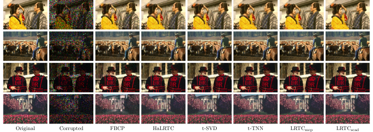
Figure 3: Tensor completion performance comparison on example images.

VI-A Datasets and Experimental Settings

We evaluate the effectiveness of the proposed non-convex tensor completion and tensor RPCA algorithms on Berkeley Segmentation 500 Dataset (BSD 500) [32] and Natural Scenes 2002 Dataset (NS 2002) [33]. Berkeley Segmentation 500 Dataset consists of 500 natural images, and Natural Scenes 2002 Dataset contains 8 hyperspectral images with 31 bands sampled from 410nm to 710nm at 10nm intervals. All the hyperspectral images are downsampled by factor 2. We employ Mean Square Error (MSE), Peak Signal-to-Noise Ratio (PSNR), Feature SIMilarity (FSIM) [34], Erreur Relative Globale Adimensionnelle de Synthèse (ERGAS)[35] and Spectral Angle Mapper (SAM) [36, 37] as performance evaluation indexes. Smaller MSE, ERGAS, SAM and larger PSNR, FSIM indicates the result is better.

There are some practical issues to clarify about Algorithm V-A and Algorithm V-B. First, the hyper-parameters $\mu_{0},\rho,\mu_{\text{max}}$ are introduced to accelerate the convergence speed. The inner ADMM iteration is always convergent regardless of the settings of these parameters, but the speed of convergence is different. In practice, we find setting $\mu_{0}=1,\rho=1.1,\mu_{\text{max}}=1e10$ results in fast convergence. Second, the initialization of $\mathcal{X}^{0}$ and $\mathcal{L},\mathcal{E}$ is very important, since a good starting position usually leads to better final result in non-convex optimization problems. We suggest initializing $\mathcal{X}^{0}$ or $\mathcal{L}^{0},\mathcal{E}^{0}$ by other tensor completion or tensor RPCA methods (such as TRPCA [23]). Last but not least, it usually takes a long time for the outer iteration to converge. In practice, it’s not necessary to wait for convergence. Instead, we can iterate the outer loop for fixed times.

TABLE I: Tensor completion performances evaluation on natural images under varying sampling rates.

Method	20%			40%			60%			80%			time (s)
	PSNR	SSIM	FSIM	PSNR	SSIM	FSIM	PSNR	SSIM	FSIM	PSNR	SSIM	FSIM
SiLRTC	$23.59$	$0.798$	$0.822$	$27.987$	$0.899$	$0.915$	$32.24$	$0.951$	$0.964$	$37.47$	$\bf 0.977$	$0.988$	$19.95$
HaLRTC	$23.82$	$0.797$	$0.828$	$28.39$	$0.902$	$0.920$	$33.038$	$0.953$	$0.968$	$39.27$	$\bf 0.978$	$0.991$	$31.32$
FBCP	$24.08$	$0.668$	$0.794$	$26.40$	$0.753$	$0.837$	$27.35$	$0.799$	$0.857$	$27.71$	$0.82$	$0.865$	$103.68$
t-SVD	$24.13$	$0.764$	$0.835$	$29.703$	$0.893$	$0.931$	$36.03$	$0.950$	$0.977$	$45.04$	$0.969$	$0.992$	$33.47$
t-TNN	$25.30$	$0.841$	$0.864$	$30.50$	$0.923$	$0.943$	$36.27$	$0.952$	$0.978$	$44.14$	$0.967$	$0.991$	$\bf 3.03$
$\text{LRTC}_{mcp}$	$\bf 25.70$	$\bf 0.845$	$\bf 0.869$	$\bf 31.06$	$\bf 0.927$	$\bf 0.946$	$\bf 36.87$	$\bf 0.959$	$\bf 0.980$	$\bf 45.46$	$0.973$	$\bf 0.993$	$3.79$
$\text{LRTC}_{scad}$	$\bf 25.70$	$\bf 0.844$	$\bf 0.869$	$\bf 31.04$	$\bf 0.926$	$\bf 0.946$	$\bf 36.84$	$\bf 0.959$	$\bf 0.980$	$\bf 45.45$	$0.973$	$\bf 0.993$	$3.83$

TABLE II: Tensor completion performances evaluation on hyperspectral images under varying sampling rates. The unit is $10^{-4}$ for MSE.

Method	20%			40%			60%			80%			time (s)
	PSNR	MSE	ERGAS	PSNR	MSE	ERGAS	PSNR	MSE	ERGAS	PSNR	MSE	ERGAS
SiLRTC	$41.71$	$4.70$	$30.912$	$45.46$	$1.95$	$21.524$	$49.14$	$0.827$	$14.412$	$52.86$	$0.354$	$10.341$	$42.21$
HaLRTC	$42.11$	$4.53$	$29.626$	$45.95$	$1.90$	$20.556$	$49.79$	$0.801$	$13.514$	$53.67$	$0.342$	$9.660$	$53.11$
FBCP	$37.09$	$14.47$	$52.931$	$43.25$	$3.85$	$29.318$	$46.00$	$2.225$	$22.344$	$46.67$	$2.011$	$20.688$	$210.18$
t-SVD	$41.64$	$5.10$	$31.835$	$45.52$	$2.12$	$22.142$	$49.42$	$0.886$	$14.685$	$53.49$	$0.365$	$10.157$	$224.21$
t-TNN	$42.46$	$3.81$	$28.702$	$46.07$	$1.60$	$20.135$	$49.82$	$0.667$	$\bf 13.272$	$53.61$	$\bf 0.290$	$\bf 9.515$	$\bf 47.29$
$\text{LRTC}_{\mathrm{mcp}}$	$\bf 42.91$	$\bf 3.58$	$\bf 27.799$	$\bf 46.75$	$\bf 1.51$	$\bf 19.684$	$\bf 50.47$	$\bf 0.665$	$\bf 13.293$	$\bf 54.11$	$\bf 0.316$	$\bf 9.642$	$70.95$
$\text{LRTC}_{\mathrm{scad}}$	$\bf 42.91$	$\bf 3.58$	$\bf 27.804$	$\bf 46.76$	$\bf 1.51$	$\bf 19.684$	$\bf 50.46$	$\bf 0.666$	$13.298$	$\bf 54.11$	$\bf 0.316$	$\bf 9.642$	$71.14$

VI-B Tensor Completion Experiments

We conduct tensor completion experiments on BSD 500 and NS 2002 to test the performances of $\text{LRTC}_{\mathrm{mcp}}$ and $\text{LRTC}_{\mathrm{scad}}$. For comparison, we also consider five competing tensor completion methods: Bayesian CP Factorization (FBCP) [3], Simple Low-Rank Tensor Completion (SiLRTC) [2], High Accuracy Low-Rank Tensor Completion (HaLRTC) [2], tensor-SVD based method (t-SVD) [21], twist Tensor Nuclear Norm based method (t-TNN) [11].

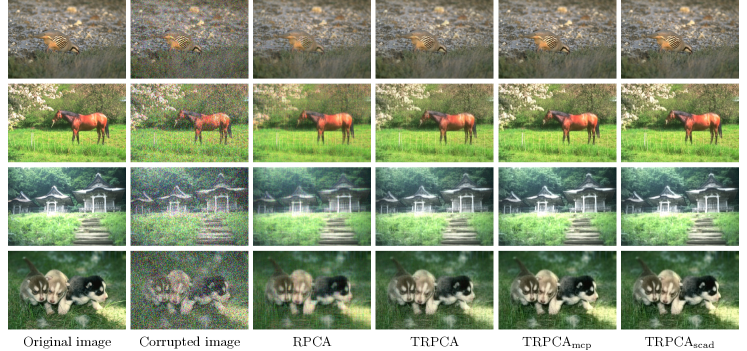
Figure 4: Tensor RPCA performance comparison on example images. From top to bottom: $p_{n}=0.1,0.2,0.3,0.4$.

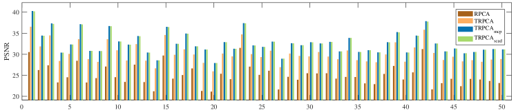
Figure 5: Comparison of PSNR values obtained by RPCA, TRPCA, $\text{TRPCA}_{\mathrm{mcp}}$,$\text{TRPCA}_{\mathrm{scad}}$ on randomly selected 50 images.

Natural image inpainting. We randomly select 200 images in BSD 500 for evaluation. For each image, pixels are randomly sampled with a sampling rate ranging from $20\%$ to $80\%$. For our $\text{LRTC}_{\mathrm{mcp}}$ and $\text{LRTC}_{\mathrm{scad}}$ models, we set $\gamma=25$, and use the result of t-TNN as initialization. To alleviate redundant computations, we apply the one-step LLA strategy [38, 24], $i.e.$, we run the outer loop only once instead of waiting for convergence. The average performances over selected 200 images under different sampling rates are summarized in Table I. From this table, we can see that our proposed $\text{LRTC}_{\mathrm{mcp}}$ and $\text{LRTC}_{\mathrm{scad}}$ outperform other competing methods in terms of all performance evaluation indices. As for efficiency, the proposed methods are significantly faster than FBCP, SiLRTC, HaLRTC, and t-SVD. Since the proposed methods are initialized by t-TNN, the running time is always slightly longer than t-TNN. However, the performances are improved by only one MM iteration and the extra running times are marginal. Therefore, we claim that it is necessary to introduce non-convexity in the tensor completion task. These observations demonstrate $\text{LRTC}_{\mathrm{mcp}}$ and $\text{LRTC}_{\mathrm{scad}}$ are both effective and efficient. We also give visual comparisons in Figure 3.

Hyperspectral image inpainting. We use all 8 hyperspectral images in this experiment. For each hyperspectral image, we randomly sample its elements with a sampling rate ranging from $0.2$ to $0.8$. Since the sizes of hyperspectral images are relatively large, we run the outer loop in Algorithm V-A for 10 iterations based on t-TNN initialization. The performance comparison are shown in Table II. We have similar observations as in the natural image case: the results obtained by $\text{LRTC}_{\mathrm{mcp}}$ and $\text{LRTC}_{\mathrm{scad}}$ have lower MSE, ERGAS, and higher PSNR, indicating that the proposed methods outperform competing methods. The fastest and the slowest algorithms are different in Table I and II mainly because $n_{3}=3$ for natural images while $n_{3}=31$ for hyperspectral images and the time complexities of these algorithms depends on $n_{3}$ differently. Besides, we find that the results of $\text{LRTC}_{\mathrm{mcp}}$ and $\text{LRTC}_{\mathrm{scad}}$ are nearly the same since MCP and SCAD shares very similar properties.

VI-C Tensor RPCA Experiments

We compare our proposed $\text{TRPCA}_{\mathrm{mcp}}$ and $\text{TRPCA}_{\mathrm{scad}}$ with matrix RPCA [9, 8] and TNN based TRPCA [10, 23] on both natural images and multispectral images. To apply matrix RPCA in tensor RPCA task, we simply apply matrix RPCA to each frontal slices of the corrupted tensor.

Natural image restoration. We first test $\text{TRPCA}_{\mathrm{mcp}}$ and $\text{TRPCA}_{\mathrm{scad}}$ on BSD 500. Each image is corrupted by salt-and-pepper noise with probability $p_{n}=0.1$. We set $\gamma_{1}=\gamma_{2}=20$ and run the outer loop of Algorithm V-B for 10 iterations. Performance comparison on randomly selected 50 images are shown in Figure 5. From this figure, we have following observations. First, the results of TRPCA,$\text{TRPCA}_{\mathrm{mcp}}$ and $\text{TRPCA}_{\mathrm{scad}}$ are significantly better than results of RPCA. This indicates that considering tensor structure helps to improve recovery quality compared to consider each channel individually. Second, $\text{TRPCA}_{\mathrm{mcp}}$ and $\text{TRPCA}_{\mathrm{scad}}$ obtained better performance than TRPCA, which means introducing concavity to Tensor RPCA tasks are necessary. Third, the PSNR values of $\text{TRPCA}_{\mathrm{mcp}}$ and $\text{TRPCA}_{\mathrm{scad}}$ are very similar, indicating the final result is not sensitive to the choice of non-convex penalty. We also give visual comparisons in Figure 4. Note that for the noise proportion ranging from $0.1$ to $0.4$ in Figure 4.

TABLE III: Tensor Robust Principal Component Analysis performances evaluation on hyper-spectral images.

$p_{n}$	Index	RPCA	TRPCA	$\text{TRPCA}_{\mathrm{mcp}}$	$\text{TRPCA}_{\mathrm{scad}}$
0.1	MSE	$20.113$	$3.680$	$\bf 3.332$	$\bf 3.329$
	PSNR	$41.89$	$46.11$	$\bf 46.57$	$\bf 46.57$
	ERGAS	$23.224$	$13.203$	$\bf 12.898$	$\bf 12.893$
	SAM	$0.0887$	$0.0894$	$\bf 0.0880$	$\bf 0.0879$
0.2	MSE	$21.298$	$4.353$	$\bf 3.837$	$\bf 3.834$
	PSNR	$41.31$	$45.63$	$\bf 46.08$	$\bf 46.09$
	ERGAS	$24.374$	$14.473$	$\bf 13.703$	$\bf 13.706$
	SAM	$0.1191$	$0.1003$	$\bf 0.0961$	$\bf 0.0961$
0.3	MSE	$26.430$	$6.637$	$\bf 4.731$	$\bf 4.726$
	PSNR	$39.68$	$44.13$	$\bf 45.28$	$\bf 45.27$
	ERGAS	$28.956$	$18.668$	$\bf 15.177$	$\bf 15.205$
	SAM	$0.1710$	$0.1291$	$\bf 0.1076$	$\bf 0.1079$
0.4	MSE	$49.858$	$28.275$	$\bf 6.979$	$\bf 6.964$
	PSNR	$36.13$	$38.51$	$\bf 43.16$	$\bf 43.11$
	ERGAS	$49.877$	$50.354$	$\bf 20.126$	$\bf 20.298$
	SAM	$0.2602$	$0.2483$	$\bf 0.1428$	$\bf 0.1440$

Hyperspectral image restoration. In this part, we test the proposed models on NS 2002. We add random noise to each hyperspectral image with probability $p_{n}$ ranging from $0.1$ to $0.4$. Here, the noise is uniformly distributed in $[0,0.1*M)$ where $M$ is the maximum absolute value of the original image. We set $\gamma_{1}=\gamma_{2}=50$, and run the outer loop for 10 iterations. The results of TRPCA are used as initialization for the proposed methods. We employ MSE, PSNR, ERGAS, and SAM as quality indexes. The results are reported in Table III. It’s easy to see that $\text{TRPCA}_{\mathrm{mcp}}$ and $\text{TRPCA}_{\mathrm{scad}}$ outperform competing methods in terms of all quality indexes. Specifically, we note that when $p_{n}=0.4$, $i.e.$, the noise proportion is rather large, the proposed methods improve the results of TRPCA significantly. In these circumstances, the sparse assumption on noise may not hold. Although RPCA and TRPCA have nice exact recovery property under certain conditions, these conditions are rather strict and sometimes not satisfied. However, the proposed methods still recover the images successfully.

VII Conclusions

In this paper, we have presented a new non-convex tensor rank surrogate function and a new non-convex sparsity measure based on the MCP and SCAD penalty functions. Then, we have analyzed some theoretical properties of the proposed penalties. In particular, we applied the non-convex penalties in tensor completion and tensor robust principal component analysis tasks, and devised optimization algorithms based on majorization minimization. Experimental results on natural images and hyperspectral images substantiate the proposed methods outperform competing methods.

Acknowledgement

This work was supported by the National Key Research and Development Program of China under grant 2018AAA0100205.

Appendix

In this supplemental material, we give detailed proofs of propositions and theorems in Section 4 and derive the ADMM steps in Section 5 of our paper.

SCAD and MCP

Although the properties of SCAD and MCP are extensively investigated in literature, we review some vital properties related to our paper here and provide proof for completeness.

Definition VII.1 (SCAD).

For some $\gamma>1$ and $\lambda>0$, the SCAD function is given by

$$\varphi^{\mathrm{SCAD}}_{\lambda,\gamma}(t)=\begin{cases}\lambda|t|\quad&\mathrm{if}|t|\leq\lambda,\\ \frac{\gamma\lambda|t|-0.5(t^{2}+\lambda^{2})}{\gamma-1}\quad&\mathrm{if}\lambda<|t|\leq\gamma\lambda,\\ \frac{\gamma+1}{2}\lambda^{2}\quad&\mathrm{if}|t|>\gamma\lambda.\end{cases}$$ (19)

Definition VII.2 (MCP).

For some $\gamma>1$ and $\lambda>0$, the MCP function is given by

$$\varphi^{\mathrm{MCP}}_{\lambda,\gamma}(t)=\begin{cases}\lambda|t|-\frac{t^{2}}{2\gamma}\quad&\mathrm{if}|t|<\gamma\lambda,\\ \frac{\gamma\lambda^{2}}{2}\quad&\mathrm{if}|t|\geq\gamma\lambda.\end{cases}$$ (20)

We use $\varphi_{\lambda,\gamma}(t)$ to denote $\varphi_{\lambda,\gamma}^{\mathrm{SCAD}}(t)$ or $\varphi_{\lambda,\gamma}^{\mathrm{MCP}}(t)$ alternatively, then we have the following properties:

Proposition VII.1.

1. $\varphi_{\lambda,\gamma}(t)\geq 0$ and $\varphi_{\lambda,\gamma}(t)=0$ if and only if $t=0$.

2. For fixed $t$ and $\lambda$, $\varphi_{\lambda,\gamma}(t)$ is increasing in $\gamma$.

3. As $\gamma\rightarrow\infty$, $\varphi_{\lambda,\gamma}(t)\rightarrow\lambda|t|$.

4. When restricted on $t\geq 0$, $\varphi_{\lambda,\gamma}(t)$ is concave.

Proof.

Note that $\varphi_{\lambda,\gamma}(t)$ is an even function, thus we only consider the case $t\geq 0$.

1. For SCAD, if $0\leq t\leq\lambda$ or $t>\gamma\lambda$, $\varphi_{\lambda,\gamma}^{\mathrm{SCAD}}(t)\geq 0$ since $\lambda>0$ and $\gamma>0$. If $\lambda<t\leq\gamma\lambda$, the minimum of $\varphi_{\lambda,\gamma}^{\mathrm{SCAD}}(t)$ is attained at $\lambda$, which equals to $\lambda^{2}$. Therefore, $\varphi_{\lambda,\gamma}^{\mathrm{SCAD}}(t)\geq 0$.

   For MCP, if $t>\lambda\gamma$ $\varphi_{\lambda,\gamma}^{\mathrm{MCP}}(t)\geq 0$ since $\lambda>0,\gamma>0$. If $t\leq\gamma\lambda$, the minimum of $\varphi_{\lambda,\gamma}^{\mathrm{MCP}}(t)$ is attained at $0$, which equals to $0$. Therefore, $\varphi_{\lambda,\gamma}^{\mathrm{MCP}}(t)\geq 0$.

   Obviously, $\varphi_{\lambda,\gamma}(t)=0$ if and only if $t=0$.

2. Suppose we have $\gamma_{2}>\gamma_{1}>1$.

   For SCAD, increasing $\gamma$ has no influence for $0\leq t\leq\lambda$. If $\lambda<t<\gamma_{1}\lambda$, then $\lambda<t<\gamma_{2}\lambda$. Note that

   $$\frac{\mathrm{d}}{\mathrm{d}\gamma}\frac{\gamma\lambda t-0.5(t^{2}+\lambda^{2})}{\gamma-1}=\frac{(t-\lambda)^{2}}{2(\gamma-1)^{2}}\geq 0.$$

   Therefore, $\varphi_{\lambda,\gamma_{2}}^{\mathrm{SCAD}}(t)\geq\varphi_{\lambda,\gamma_{1}}^{\mathrm{SCAD}}(t)$. If $t>\gamma_{1}\lambda$, then we have two cases: $t>\gamma_{2}\lambda$ or $\lambda<t\leq\gamma_{2}\lambda$. If $t>\gamma_{2}\lambda$, then $\varphi_{\lambda,\gamma_{2}}^{\mathrm{SCAD}}(t)=\frac{\gamma_{2}+1}{2}\lambda^{2}>\frac{\gamma_{1}+1}{2}\lambda^{2}=\varphi_{\lambda,\gamma_{1}}^{\mathrm{SCAD}}(t)$. If $\lambda<t\leq\gamma_{2}\lambda$, then

   $$\varphi_{\lambda,\gamma_{2}}^{\mathrm{SCAD}}(t)-\varphi_{\lambda,\gamma_{1}}^{\mathrm{SCAD}}(t)=\frac{\gamma_{2}\lambda t-0.5(t^{2}+\lambda^{2})}{\gamma_{2}-1}-\frac{\gamma_{1}+1}{2}\lambda^{2}=\frac{-t^{2}+2\gamma_{2}\lambda t-\lambda^{2}-(\gamma_{1}+1)(\gamma_{2}-1)\lambda^{2}}{2(\gamma_{2}-1)}.$$

   Note that in this case $\gamma_{1}\lambda\leq t\leq\gamma_{2}\lambda$, the above equation attains its minimum at $\gamma_{1}\lambda$, thus

   $$\varphi_{\lambda,\gamma_{2}}^{\mathrm{SCAD}}(t)-\varphi_{\lambda,\gamma_{1}}^{\mathrm{SCAD}}(t)\geq\frac{(\gamma_{2}-\gamma_{1})(\gamma_{1}-1)\lambda^{2}}{2(\gamma_{2}-1)}>0.$$

   The last inequality follows from the condition $\gamma_{2}>\gamma_{1}>1$. Therefore, we conclude that $\varphi_{\lambda,\gamma}^{\mathrm{SCAD}}(t)$ is increasing with respect to $\gamma$.

   For MCP, if $0\leq t<\gamma_{1}\lambda$, then $0\leq t<\gamma_{2}\lambda$, thus $\varphi_{\lambda,\gamma_{2}}^{\mathrm{MCP}}(t)=\lambda t-\frac{t^{2}}{2\gamma_{2}}>\lambda t-\frac{t^{2}}{2\gamma_{1}}=\varphi_{\lambda,\gamma_{1}}^{\mathrm{MCP}}(t)$. If $t\geq\gamma_{1}\lambda$, we have two cases: $t\geq\gamma_{2}\lambda$ or $0<t<\gamma_{2}\lambda$. If $t\geq\gamma_{2}\lambda$, then $\varphi_{\lambda,\gamma_{2}}^{\mathrm{MCP}}(t)=\frac{\gamma_{2}\lambda^{2}}{2}>\frac{\gamma_{1}\lambda^{2}}{2}=\varphi_{\lambda,\gamma_{1}}^{\mathrm{MCP}}(t)$. If $0\leq t\leq\gamma_{2}\lambda$, then

   $$\varphi_{\lambda,\gamma_{2}}^{\mathrm{MCP}}(t)-\varphi_{\lambda,\gamma_{1}}^{\mathrm{MCP}}(t)=\lambda t-\frac{t^{2}}{2\gamma_{2}}-\frac{\gamma_{1}\lambda^{2}}{2}>\frac{(\gamma_{2}-\gamma_{1})\gamma_{1}\lambda^{2}}{2\gamma_{2}}>0.$$

   Therefore, we conclude that $\varphi_{\lambda,\gamma}^{\mathrm{MCP}}(t)$ is increasing with respect to $\gamma$.

3. Note that as $\gamma\rightarrow\infty$,

   $$\frac{\gamma\lambda|t|-0.5(t^{2}+\lambda^{2})}{\gamma-1}\rightarrow\lambda|t|\quad,\quad\lambda|t|-\frac{t^{2}}{2\gamma}\rightarrow\lambda|t|.$$

   The result follows easily.

4. Consider the second order derivative of $\varphi_{\lambda,\gamma}(t)$.

   For SCAD,

   $$\frac{\mathrm{d}^{2}}{\mathrm{d}^{2}t}\varphi_{\lambda,\gamma}^{\mathrm{SCAD}}(t)=\begin{cases}0,\quad\text{if }0\leq t\leq\lambda\text{ or }t>\gamma\lambda,\\ -\frac{1}{\gamma-1},\quad\text{if }t\leq\gamma\lambda.\end{cases}$$

   For MCP,

   $$\frac{\mathrm{d}^{2}}{\mathrm{d}^{2}t}\varphi_{\lambda,\gamma}^{\mathrm{MCP}}(t)=\begin{cases}-\frac{1}{\gamma},\quad\text{if }0\leq t\leq\gamma\lambda,\\ 0,\quad\text{if }t\geq\gamma\lambda.\end{cases}$$

   Therefore, $\varphi_{\lambda,\gamma}(t)$ is concave over $[0,\infty)$ since the second order derivative is non-positive. Besides, by the definition of concave function we know that $\varphi_{\lambda,\gamma}(t)\leq\varphi_{\lambda,\gamma}(s)+\varphi_{\lambda,\gamma}^{\prime}(s)(t-s)$ for $s,t\geq 0$.

∎

A Novel Tensor Sparsity Measure

Recall that the novel tensor sparsity measure is defined as

$$\Phi_{\lambda,\gamma}(\mathcal{A})=\sum_{i=1}^{n_{1}}\sum_{j=1}^{n_{2}}\sum_{k=1}^{n_{3}}\varphi_{\lambda,\gamma}(\mathcal{A}_{ijk}).$$ (21)

Here, we may set $\varphi_{\lambda,\gamma}$ to be $\varphi^{\mathrm{SCAD}}_{\lambda,\gamma}$ or $\varphi^{\mathrm{MCP}}_{\lambda,\gamma}$. We have the following proposition:

Proposition VII.2.

For $\mathcal{A}\in\mathbb{R}^{n_{1}\times n_{2}\times n_{3}}$, $\Phi_{\lambda,\gamma}(\mathcal{A})$ satisfies:

1. $\Phi_{\lambda,\gamma}(\mathcal{A})\geq 0$ with the equality holds iff $\mathcal{A}=0$;

2. $\Phi_{\lambda,\gamma}(\mathcal{A})$ is concave with respect to $|\mathcal{A}|$;

3. $\Phi_{\lambda,\gamma}(\mathcal{A})$ is increasing in $\gamma$, $\Phi_{\lambda,\gamma}(\mathcal{A})\leq\lambda\|\mathcal{A}\|_{1}$ and $\lim_{\gamma\rightarrow\infty}\Phi_{\lambda,\gamma}(\mathcal{A})=\lambda\|\mathcal{A}\|_{1}$.

Proof.

Note that $\Phi_{\lambda,\gamma}(\mathcal{A})$ is separable with respect to each entry of $\mathcal{A}$. Thus, applying the related properties of $\varphi_{\lambda,\gamma}(t)$ to each entry $\mathcal{A}_{ijk}$, we immediately get the result. ∎

A Novel Tensor Rank Penalty

Suppose $\mathcal{A}$ has t-SVD $\mathcal{A}=\mathcal{U}*\mathcal{S}*\mathcal{V}^{*}$, we define the $\gamma-$norm of $\mathcal{A}$ as

$$\|\mathcal{A}\|_{\gamma}=\frac{1}{n_{3}}\sum_{i,k}\varphi_{1,\gamma}(\overline{\mathcal{S}}(i,i,k)).$$ (22)

The tensor $\gamma-$norm enjoys the following properties.

Proposition VII.3.

For $\mathcal{A}\in\mathbb{R}^{n_{1}\times n_{2}\times n_{3}}$, suppose $\mathcal{A}$ has t-SVD $\mathcal{A}=\mathcal{U}*\mathcal{S}*\mathcal{V}^{*}$, then $\|\mathcal{A}\|_{\gamma}$ satisfies:

1. $\|\mathcal{A}\|_{\gamma}\geq 0$ with equality holds iff $\mathcal{A}=0$;

2. $\|\mathcal{A}\|_{\gamma}$ is increasing in $\gamma$, $\|\mathcal{A}\|_{\gamma}\leq\|\mathcal{A}\|_{*}$ and $\lim_{\gamma\rightarrow\infty}\|\mathcal{A}\|_{\gamma}=\|\mathcal{A}\|_{*}$;

3. $\|\mathcal{A}\|_{\gamma}$ is concave with respect to $\{\overline{\mathcal{S}}(i,i,k)\}_{i,k}$;

4. $\|\mathcal{A}\|_{\gamma}$ is orthogonal invariant, $i.e.$, for any orthogonal tensors $\mathcal{P}\in\mathbb{R}^{n_{1}\times n_{1}\times n_{3}},\mathcal{Q}\in\mathbb{R}^{n_{2}\times n_{2}\times n_{3}}$, $\|\mathcal{P}*\mathcal{A}*\mathcal{Q}\|_{\gamma}=\|\mathcal{A}\|_{\gamma}$.

Proof.

1. Since $\varphi_{1,\gamma}(t)\geq 0$ and $\|\mathcal{A}\|_{\gamma}$ is the sum of $\varphi_{1,\gamma}(t)$, we immediately know $\|\mathcal{A}\|_{\gamma}\geq 0$. If $\mathcal{A}=0$, then obviously $\mathcal{S}=0$ and $\overline{\mathcal{S}}=0$, which implies $\|\mathcal{A}\|_{\gamma}=0$. On the other hand, $\|\mathcal{A}\|_{\gamma}=0$ implies $\overline{\mathcal{S}}(i,i,k)=0$. However, $\overline{\mathcal{S}}$ is f-diagonal, thus $\overline{\mathcal{S}}=0$, and $\mathcal{A}=\mathcal{U}*\texttt{ifft}(\overline{\mathcal{S}},3)*\mathcal{V}^{*}=0$.

2. Since $\varphi_{1,\gamma}(t)$ is increasing with respect to $\gamma$ and $\|\mathcal{A}\|_{\gamma}$ is the sum of $\varphi_{1,\gamma}(t)$, using the properties of $\varphi_{\lambda,\gamma}(t)$ we know $\|\mathcal{A}\|_{\gamma}$ is increasing with respect to $\gamma$ and

   $$\lim_{\gamma\rightarrow\infty}\|\mathcal{A}\|_{\gamma}=\lim_{\gamma\rightarrow\infty}\frac{1}{n_{3}}\sum_{i,k}\varphi_{1,\gamma}(\overline{\mathcal{S}}(i,i,k))=\frac{1}{n_{3}}\sum_{i,k}|\overline{\mathcal{S}}(i,i,k)|=\|\mathcal{A}\|_{*}.$$

   Combining the above facts, we also get $\|\mathcal{A}\|_{\gamma}\leq\|\mathcal{A}\|_{*}.$

3. This follows from the fact that $\varphi_{\lambda,\gamma}(t)$ is concave over $[0,\infty).$

4. Since $\mathcal{A}$ has t-SVD $\mathcal{A}=\mathcal{U}*\mathcal{S}*\mathcal{V}^{*}$, we claim that $\mathcal{P}*\mathcal{U}*\mathcal{S}*\mathcal{V}^{*}*\mathcal{Q}^{*}$ is the t-SVD of $\mathcal{P}*\mathcal{A}*\mathcal{Q}^{*}$. $\mathcal{S}$ is already f-diagonal, so we only need to verify $\mathcal{P}*\mathcal{U}$ and $(\mathcal{V}^{*}*\mathcal{Q}^{*})^{*}=\mathcal{Q}*\mathcal{V}$ are orthogonal.

   $$(\mathcal{P}*\mathcal{U})*(\mathcal{P}*\mathcal{U})^{*}=\mathcal{P}*\mathcal{U}*\mathcal{U}^{*}*\mathcal{P}=\mathcal{I}.$$

   Other equalities are similar to verify. Therefore, $\|\mathcal{P}*\mathcal{A}*\mathcal{Q}^{*}\|_{\gamma}=\frac{1}{n_{3}}\sum_{i,k}\varphi_{1,\gamma}(\overline{\mathcal{S}}(i,i,k))=\|\mathcal{A}\|_{\gamma}$.

∎

Generalized Thresholding Operators

Theorem VII.4.

We can view $\Phi_{\lambda,\mu}(\mathcal{X})$ as a function of $|\mathcal{X}|$, and $\|\mathcal{X}\|_{\gamma}$ as a function of $\{\overline{\mathcal{S}}(i,i,k)\}_{i,k}$. For any $\mathcal{X}^{\textnormal{old}}$, let

$$Q_{\lambda,\gamma}(\mathcal{X}|\mathcal{X}^{\textnormal{old}})=\Phi_{\lambda,\gamma}(\mathcal{X}^{\textnormal{old}})+\sum_{i,j,k}\varphi^{\prime}_{\lambda,\gamma}(|\mathcal{X}^{\textnormal{old}}_{ijk}|)(|\mathcal{X}_{ijk}|-|\mathcal{X}^{old}_{ijk}|),$$

$$Q_{\gamma}(\mathcal{X}|\mathcal{X}^{\textnormal{old}})=\|\mathcal{X}^{\textnormal{old}}\|_{\gamma}+\frac{1}{n_{3}}\sum_{i,k}\varphi_{1,\gamma}^{\prime}(\overline{\mathcal{S}}^{\textnormal{old}}_{iik})(\overline{\mathcal{S}}_{iik}-\overline{\mathcal{S}}^{\textnormal{old}}_{iik}),$$

then

$$Q_{\lambda,\gamma}(\mathcal{X}^{\mathrm{old}}|\mathcal{X}^{\mathrm{old}})=\Phi_{\lambda,\gamma}(\mathcal{X}^{\mathrm{old}})\qquad,\qquad\Phi_{\lambda,\gamma}(\mathcal{X})\leq Q_{\lambda,\gamma}(\mathcal{X}|\mathcal{X}^{\textnormal{old}}),$$ (23)

$$Q_{\gamma}(\mathcal{X}^{\mathrm{old}}|\mathcal{X}^{\mathrm{old}})=\|\mathcal{X}^{\mathrm{old}}\|_{\gamma}\qquad,\qquad\|\mathcal{X}\|_{\gamma}\leq Q_{\gamma}(\mathcal{X}|\mathcal{X}^{\textnormal{old}}).$$

Proof.

Recall that for any $s,t\geq 0$ we have $\varphi_{\lambda,\gamma}(t)\leq\varphi_{\lambda,\gamma}(s)+\varphi_{\lambda,\gamma}(s)(t-s)$.

$$\Phi_{\lambda,\gamma}(\mathcal{X})=\sum_{i,j,k}\varphi_{\lambda,\gamma}(\mathcal{X}_{ijk})=\sum_{i,j,k}\varphi_{\lambda,\gamma}(|\mathcal{X}_{ijk}|)\leq\sum_{i,j,k}\left(\varphi_{\lambda,\gamma}(|\mathcal{X}^{\textnormal{old}}_{ijk}|)+\varphi_{\lambda,\gamma}^{\prime}(|\mathcal{X}^{\textnormal{old}}_{ijk}|)(|\mathcal{X}_{ijk}|-|\mathcal{X}^{\textnormal{old}}_{ijk}|)\right)=Q_{\lambda,\gamma}(\mathcal{X}|\mathcal{X}^{\textnormal{old}}).$$

$$\|\mathcal{X}\|_{\gamma}=\frac{1}{n_{3}}\sum_{i,k}\varphi_{1,\gamma}(\overline{\mathcal{S}}_{ijk})\leq\frac{1}{n_{3}}\sum_{i,k}\left(\varphi_{1,\gamma}(\overline{\mathcal{S}}^{\textnormal{old}}_{ijk})+\varphi_{1,\gamma}^{\prime}(\overline{\mathcal{S}}^{\textnormal{old}}_{ijk})(\overline{\mathcal{S}}_{ijk}-\overline{\mathcal{S}}_{ijk}^{\textnormal{old}})\right)=Q_{\gamma}(\mathcal{X}|\mathcal{X}^{\textnormal{old}}).$$

∎

In the following soft thresholding operator is defined as $\mathcal{T}_{\lambda}(z)=\textnormal{sgn}(z)[|z|-\lambda]_{+}$, which is the proximal operator of $\ell_{1}-$norm.

Definition VII.3 (Generalized soft thresholding).

Suppose $\mathcal{X},\mathcal{W}\in\mathbb{R}^{n_{1}\times n_{2}\times n_{3}}$, the generalized soft thresholding operator is defined as

$$[\mathcal{T}_{\mathcal{W}}(\mathcal{X})]_{ijk}=\mathcal{T}_{\mathcal{W}_{ijk}}(\mathcal{X}_{ijk}).$$ (24)

Theorem VII.5.

For $\forall\mu>0$, let $\mathcal{W}_{ijk}=\varphi_{\lambda,\gamma}^{\prime}(|\mathcal{X}^{\textnormal{old}}_{ijk}|)/\mu$, then

$$\mathcal{T}_{\mathcal{W}}(\mathcal{Y})=\arg\min_{\mathcal{X}}Q_{\lambda,\gamma}(\mathcal{X}|\mathcal{X}^{\textnormal{old}})+\frac{\mu}{2}\|\mathcal{X}-\mathcal{Y}\|_{F}^{2}.$$ (25)

Proof.

In fact,

$$\arg\min_{\mathcal{X}}Q_{\lambda,\gamma}(\mathcal{X}|\mathcal{X}^{\textnormal{old}})+\frac{\mu}{2}\|\mathcal{X}-\mathcal{Y}\|_{F}^{2}= \arg\min_{\mathcal{X}}\sum_{ijk}\varphi_{\lambda,\gamma}^{\prime}(|\mathcal{X}^{\textnormal{old}}_{ijk}|)|\mathcal{X}_{ijk}|+\frac{\mu}{2}\|\mathcal{X}-\mathcal{Y}\|_{F}^{2}$$

$$= \arg\min_{\mathcal{X}}\sum_{i,j,k}\left(\varphi_{\lambda,\gamma}^{\prime}(|\mathcal{X}^{\textnormal{old}}_{ijk}|)|\mathcal{X}_{ijk}|+\frac{\mu}{2}(\mathcal{X}_{ijk}-\mathcal{Y}_{ijk})^{2}\right),$$

which is separable to each entries of $\mathcal{X}$. Consider $\mathcal{X}_{ijk}$, according to the property of soft thresholding operator, the minimum of $\varphi_{\lambda,\gamma}^{\prime}(|\mathcal{X}^{\textnormal{old}}|)|\mathcal{X}_{ijk}|+\frac{\mu}{2}(\mathcal{X}_{ijk}-\mathcal{Y}_{ijk})^{2}$ is attained at $\mathcal{T}_{\varphi_{\lambda,\gamma}^{\prime}(|\mathcal{X}^{\textnormal{old}}_{ijk}|)/\mu}(\mathcal{Y}_{ijk})$. Therefore, let $\mathcal{W}_{ijk}=\varphi_{\lambda,\gamma}^{\prime}(|\mathcal{X}^{\textnormal{old}}_{ijk}|)/\mu$, by the definition of generalized soft thresholding, we immediately get

$$\mathcal{T}_{\mathcal{W}}(\mathcal{Y})=\arg\min_{\mathcal{X}}Q_{\lambda,\gamma}(\mathcal{X}|\mathcal{X}^{\textnormal{old}})+\frac{\mu}{2}\|\mathcal{X}-\mathcal{Y}\|_{F}^{2}.$$

∎

Definition VII.4 (Generalized t-SVT).

Suppose a 3-way tensor $\mathcal{Y}$ has t-SVD $\mathcal{Y}=\mathcal{U}*\mathcal{S}*\mathcal{V}^{*}$, $\mathcal{W}$ is a tensor with the same shape of $\mathcal{Y}$, the generalized tensor singular value thresholding operator is defined as

$$\mathcal{D}_{\mathcal{W}}(\mathcal{Y})=\mathcal{U}*\tilde{\mathcal{S}}*\mathcal{V}^{*},$$ (26)

where $\tilde{\mathcal{S}}=\textnormal{{ifft}}(\mathcal{T}_{\mathcal{W}}(\overline{\mathcal{S}}),3)$.

Theorem VII.6.

For $\forall\mu>0$, let $\mathcal{W}_{ijk}=\delta_{i}^{j}\varphi_{1,\gamma}^{\prime}(\overline{\mathcal{S}}^{\textnormal{old}}_{iik})/\mu$ where $\delta_{i}^{j}$ is the Kronecker symbol, then

$$\mathcal{D}_{\mathcal{W}}(\mathcal{Y})=\arg\min_{\mathcal{X}}Q_{\gamma}(\mathcal{X}|\mathcal{X}^{\textnormal{old}})+\frac{\mu}{2}\|\mathcal{X}-\mathcal{Y}\|_{F}^{2}.$$ (27)

Proof.

In fact,

$$\arg\min_{\mathcal{X}}Q_{\gamma}(\mathcal{X}|\mathcal{X}^{\textnormal{old}})+\frac{\mu}{2}\|\mathcal{X}-\mathcal{Y}\|_{F}^{2}= \arg\min_{\mathcal{X}}\frac{1}{n_{3}}\sum_{i,k}\varphi_{1,\gamma}^{\prime}(\overline{\mathcal{S}}^{\textnormal{old}}_{iik})\overline{\mathcal{S}}_{iik}+\frac{\mu}{2}\|\mathcal{X}-\mathcal{Y}\|_{F}^{2}$$

$$= \arg\min_{\mathcal{X}}\frac{1}{n_{3}}\sum_{i,k}\varphi_{1,\gamma}^{\prime}(\overline{\mathcal{S}}^{\textnormal{old}}_{iik})\overline{\mathcal{S}}_{iik}+\frac{\mu}{2n_{3}}\sum_{k}\|\overline{X}^{(k)}-\overline{Y}^{(k)}\|_{F}^{2}$$

$$= \arg\min_{\mathcal{X}}\frac{1}{n_{3}}\sum_{k}\left(\sum_{i}\varphi_{1,\gamma}^{\prime}(\overline{\mathcal{S}}^{\textnormal{old}}_{iik})\overline{S}^{(k)}_{i,i}+\frac{\mu}{2}\|\overline{X}^{(k)}-\overline{Y}^{(k)}\|_{F}^{2}\right).$$

This optimization problem is separable in transformation domain with respect to each slice. Consider the subproblem of minimizing $\sum_{k}\varphi_{1,\gamma}^{\prime}(\overline{\mathcal{S}}^{\textnormal{old}}_{iik})\overline{S}^{(k)}_{i,i}+\frac{\mu}{2}\|\overline{X}^{(k)}-\overline{Y}^{(k)}\|_{F}^{2}$, suppose $\mathcal{Y}$ has t-SVD $\mathcal{Y}=\mathcal{U}*\mathcal{R}*\mathcal{V}$ or equivalently $\overline{Y}=\overline{U}\,\overline{R}\,\overline{T}^{*}$, we have

$$\sum_{k}\varphi_{1,\gamma}^{\prime}(\overline{\mathcal{S}}^{\textnormal{old}}_{iik})\overline{S}^{(k)}_{i,i}+\frac{\mu}{2}\|\overline{X}^{(k)}-\overline{Y}^{(k)}\|_{F}^{2}= \sum_{k}\varphi_{1,\gamma}^{\prime}(\overline{\mathcal{S}}^{\textnormal{old}}_{iik})\overline{S}^{(k)}_{i,i}+\frac{\mu}{2}\|\overline{X}^{(k)}-\overline{U}^{(k)}\,\overline{R}^{(k)}\,(\overline{V}^{(k)})^{*}\|_{F}^{2}$$

$$= \sum_{k}\varphi_{1,\gamma}^{\prime}(\overline{\mathcal{S}}^{\textnormal{old}}_{iik})\overline{S}^{(k)}_{i,i}+\frac{\mu}{2}\|(\overline{U}^{(k)})^{*}\overline{X}^{(k)}\overline{V}^{(k)}-\,\overline{R}^{(k)}\,\|_{F}^{2}.$$

However, note that $\overline{S}^{(k)}_{i,i}$ is still the singular values of $(\overline{U}^{(k)})^{*}\overline{X}^{(k)}\overline{V}^{(k)}$, simple calculation reveals that we obtain the minimum if $(\overline{U}^{(i)})^{*}\overline{X}^{(k)}\overline{V}^{(k)}$ is diagonal with $i$-th diagonal element equals to $\mathcal{T}_{\varphi_{1,\gamma}^{\prime}(\overline{S^{\textnormal{old}}_{iik}})/\mu}(\overline{R}^{k}_{i,i})$. That is, let $W$ be a matrix with $W_{i,j}^{(k)}=\delta_{i}^{j}\varphi_{1,\gamma}^{\prime}(\overline{S^{\textnormal{old}}_{iik}})/\mu$, then $\overline{X}=\overline{U}\mathcal{T}_{W}{\overline{R}}\,\overline{V}$. Transform back to original domain, by the definition of generalized t-SVT, we get $\mathcal{X}=\mathcal{U}*\tilde{\mathcal{S}}*\mathcal{V}^{*}$ where $\tilde{\mathcal{S}}=\texttt{ifft}(\mathcal{T}_{\mathcal{W}}(\overline{\mathcal{R}}),3)$ and $\mathcal{W}_{ijk}=\delta_{i}^{j}\varphi_{1,\gamma}^{\prime}(\overline{\mathcal{S}}^{\textnormal{old}}_{iik})/\mu$. ∎

ADMM for Proposed Non-convex Tensor Recovery Models and Algorithms

Lemma VII.7.

Suppose $\phi:I\subset\mathbb{R}\rightarrow\mathbb{R}$ is a monotone non-decreasing differentiable concave function and $x_{*}\in I$ satisfies $x_{*}\in\arg\min_{x\in I}\phi(x_{*})+\phi^{\prime}(x_{*})(x-x_{*})$, then $x_{*}$ is a minimal point of $\phi(x)$ on $I$.

Proof.

Note that $\phi(x_{*})\leq\phi(x_{*})+\phi^{\prime}(x_{*})(x-x_{*})$ for $x\in I$ indicates $\phi^{\prime}(x_{*})(x-x_{*})\geq 0,\forall x\in I$. Since $\phi$ is monotone non-decreasing, $(x-x_{*})(\phi(x)-\phi(x_{*}))\geq 0$. Multiplying these two inequalities, we obtain $\phi^{\prime}(x_{*})(\phi(x)-\phi(x_{*}))(x-x_{*})^{2}\geq 0$. Therefore, for any $x\neq x_{*}$, $\phi^{\prime}(x_{*})(\phi(x)-\phi(x_{*}))\geq 0$. If $\phi^{\prime}(x_{*})>0$, we immediately have $\phi(x)\geq\phi(x_{*})$. If $\phi^{\prime}(x_{*})=0$, then obviously $x_{*}$ is a minimizer. ∎

Remark: The SCAD and MCP functions are monotone non-decreasing on $[0,\infty)$, thus the lemma can be applied to them. Furthermore, $\Phi_{\lambda,\gamma}(\mathcal{X})$ is separable regarded as a function of $\mathcal{X}$, and $\|\mathcal{X}\|_{\gamma}$ is separable regarded as a function of $\{\overline{S}(i,i,k)\}_{i,k}$. Therefore, the lemma can also be applied to $\Phi_{\lambda,\gamma}(\mathcal{X})$ and $\|\mathcal{X}\|_{\gamma}$.

VII-A ADMM for Non-convex Tensor Completion

Consider problem

$$\min_{\mathcal{X}\in D}Q_{\gamma}(\mathcal{M}|\mathcal{X}^{\textnormal{old}})\quad\text{s.t. }\mathcal{M}=\mathcal{X}.$$ (28)

The augmented Lagrangian function is given by

$$L(\mathcal{M},\mathcal{X},\mathcal{Y})=Q_{\gamma}(\mathcal{M}|\mathcal{X}^{\textnormal{old}})+\langle\mathcal{M}-\mathcal{X},\mathcal{Y}\rangle+\frac{\mu}{2}\|\mathcal{M}-\mathcal{X}\|_{F}^{2}.$$ (29)

According to the ADMM algorithm, we have the following iteration scheme:

$$\mathcal{M}_{l+1}=\arg\min_{\mathcal{M}}Q_{\gamma}(\mathcal{M}|\mathcal{X}^{\textnormal{old}})+\frac{\mu}{2}\|\mathcal{M}-(\mathcal{X}_{l}-\frac{1}{\mu}\mathcal{Y}_{l})\|_{F}^{2},$$

$$\mathcal{X}_{l+1}=\arg\min_{\mathcal{X}\in D}\|\mathcal{X}-(\mathcal{M}_{l+1}+\frac{1}{\mu}\mathcal{Y}_{l})\|_{F}^{2},$$ (30)

$$\mathcal{Y}_{l+1}=\mathcal{Y}_{k}+\mu(\mathcal{M}_{l+1}-\mathcal{X}_{l+1}).$$

The sub-problem of updating $\mathcal{M}_{l+1}$ can be solved by generalized t-SVT as indicated in Theorem VII.6. The sub-problem of updating $\mathcal{X}_{l+1}$ has a closed-form solution: $\mathcal{X}_{l+1}=(\mathcal{M}_{l+1}+\frac{1}{\mu}\mathcal{Y})\circledast(1-\Omega)+\mathcal{O}\circledast\Omega$, where $\circledast$ is element-wise product.

Theorem VII.8.

The iteration sequence generated by $\mathcal{X}^{t+1}\in\arg\min_{\mathcal{O}_{\Omega}=\mathcal{X}_{\Omega}}Q_{\gamma}(\mathcal{X}|\mathcal{X}^{t})$ is non-increasing, $i.e.$, $\|\mathcal{X}^{t+1}\|_{\gamma}\leq\|\mathcal{X}^{t}\|_{\gamma}$ and converges to some $Q^{*}$. Besides, there exists a subsequence $\{\mathcal{X}^{i_{k}}\}_{k=1}^{\infty}$ converges to a minimal point $\mathcal{X}_{*}$ of $\|\mathcal{X}\|_{\gamma}$ on $\{\mathcal{X}|\mathcal{O}_{\Omega}=\mathcal{X}_{\Omega}\}$.

Proof.

Since $Q_{\gamma}(\mathcal{X}^{t}|\mathcal{X}^{t})=\|\mathcal{X}^{t}\|_{\gamma}$ and $\mathcal{X}^{t+1}\in\arg\min_{\mathcal{O}_{\Omega}=\mathcal{X}_{\Omega}}Q_{\gamma}(\mathcal{X}|\mathcal{X}^{t})$, we immediately have $Q_{\gamma}(\mathcal{X}^{t+1}|\mathcal{X}^{t})\leq\|\mathcal{X}^{t}\|_{\gamma}$. On the other hand, $\|\mathcal{X}^{t+1}\|_{\gamma}\leq Q_{\gamma}(\mathcal{X}^{t+1}|\mathcal{X}^{t})$, thus $\|\mathcal{X}^{t+1}\|_{\gamma}\leq\|\mathcal{X}^{t}\|_{\gamma}$.

The sequence $\{\|\mathcal{X}^{t}\|_{\gamma}\}_{l=0}^{\infty}$ is bounded below by $0$ and non-increasing, therefore converges to some limit point $Q^{*}\geq 0$.

Besides, $\{\mathcal{X}^{t}\}_{t=0}^{\infty}$ lie in the compact set $\{\mathcal{X}|\|\mathcal{X}\|_{\gamma}\leq\|\mathcal{X}^{0}\|_{\gamma}\}$, so there exists a subsequence $\{\mathcal{X}^{i_{k}}\}_{k=1}^{\infty}$ that is convergent. Without loss of generality, we assume $\mathcal{X}^{i_{k}}\rightarrow\mathcal{X}_{*}$, then we must have $\mathcal{X}_{*}\in\arg\min_{\mathcal{O}_{\Omega}=\mathcal{X}_{\Omega}}Q_{\gamma}(\mathcal{X}|\mathcal{X}_{*})$. Then by Lemma VII.7, we conclude that $\mathcal{X}_{*}$ is a minimizer of $\|\mathcal{X}\|_{\gamma}$ on $\{\mathcal{X}|\mathcal{O}_{\Omega}=\mathcal{X}_{\Omega}\}$. ∎

VII-B ADMM for Non-convex Tensor Robust PCA

Consider problem

$$\min_{\mathcal{L},\mathcal{E}}Q_{\gamma_{1}}(\mathcal{L}|\mathcal{L}^{\textnormal{old}})+Q_{\lambda,\gamma_{2}}(\mathcal{E}|\mathcal{E}^{\textnormal{old}})\quad\text{s.t. }\mathcal{L}+\mathcal{E}=\mathcal{X}.$$ (31)

The augmented Lagrangian function is

$$L(\mathcal{L},\mathcal{E},\mathcal{Y})=Q_{\gamma_{1}}(\mathcal{L}|\mathcal{L}^{\textnormal{old}})+Q_{\lambda,\gamma_{2}}(\mathcal{E}|\mathcal{E}^{\textnormal{old}})+\langle\mathcal{Y},\mathcal{L}+\mathcal{E}-\mathcal{X}\rangle+\frac{\mu}{2}\|\mathcal{L}+\mathcal{E}-\mathcal{X}\|_{F}^{2}.$$ (32)

According to the ADMM algorithm, we may iterate variables as following:

$$\mathcal{L}_{l+1}\!=\!\arg\min_{\mathcal{L}}Q_{\gamma_{1}}(\mathcal{L}|\mathcal{L}^{\textnormal{old}})+\frac{\mu}{2}\|\mathcal{L}\!-\!(\mathcal{X}\!-\!(\mathcal{E}_{l}\!+\!\frac{1}{\mu}\mathcal{Y}_{l}))\|_{F}^{2},$$

$$\mathcal{E}_{l+1}\!=\!\arg\min_{\mathcal{E}}Q_{\lambda,\gamma_{2}}(\mathcal{E}|\mathcal{E}^{\textnormal{old}})\!+\!\frac{\mu}{2}\|\mathcal{E}\!-\!(\mathcal{X}\!-\!(\mathcal{L}_{l+1}\!+\!\frac{1}{\mu}\mathcal{Y}_{l}))\|_{F}^{2},$$

$$\mathcal{Y}_{l+1}=\mathcal{Y}_{l}+\mu(\mathcal{L}_{l+1}+\mathcal{E}_{l+1}-\mathcal{X}).$$ (33)

The sub-problem of updating $\mathcal{L}$ and $\mathcal{E}$ has closed-form solutions using Theorem VII.5 and Theorem VII.6.

Theorem VII.9.

The iteration sequence generated by

$$(\mathcal{L}^{t+1},\mathcal{E}^{t+1})\in\arg\min_{\mathcal{L}+\mathcal{E}=\mathcal{X}}Q_{\gamma_{1}}(\mathcal{L}|\mathcal{L}^{t})+Q_{\lambda,\gamma_{2}}(\mathcal{E}|\mathcal{E}^{t})$$

is non-increasing, $i.e.$, $\|\mathcal{L}^{t+1}\|_{\gamma_{1}}+\Phi_{\lambda,\gamma_{2}}(\mathcal{E}^{t+1})\leq\|\mathcal{L}^{t}\|_{\gamma_{1}}+\Phi_{\lambda,\gamma_{2}}(\mathcal{E}^{t})$ and converges to some $Q^{*}$. Besides, there exists a subsequence $\{(\mathcal{L}^{i_{k}},\mathcal{E}^{i_{k}})\}_{k=1}^{\infty}$ converges to a minimal point $(\mathcal{L}_{*},\mathcal{E}_{*})$ of $\|\mathcal{L}\|_{\gamma_{1}}+\Phi_{\lambda,\gamma_{2}}(\mathcal{E})$ on $\{(\mathcal{L},\mathcal{E})|\mathcal{L}+\mathcal{E}=\mathcal{X}\}$.

Proof.

Since $Q_{\gamma_{1}}(\mathcal{L}^{t}|\mathcal{L}^{t})=\|\mathcal{L}^{t}\|_{\gamma},Q_{\lambda,\gamma_{2}}(\mathcal{E}^{t}|\mathcal{E}^{t})=\Phi_{\lambda,\gamma_{2}}(\mathcal{E}_{l})$, and $(\mathcal{L}^{t+1},\mathcal{E}^{t+1})\in\arg\min_{\mathcal{L}+\mathcal{E}=\mathcal{X}}Q_{\gamma_{1}}(\mathcal{L}|\mathcal{L}^{t})+Q_{\lambda,\gamma_{2}}(\mathcal{E}|\mathcal{E}^{t})$, we immediately have $Q_{\gamma_{1}}(\mathcal{L}^{t+1}|\mathcal{L}^{t})+Q_{\lambda,\gamma_{2}}(\mathcal{E}^{t+1}|\mathcal{E}^{t})\leq\|\mathcal{L}^{t}\|_{\gamma_{1}}+\leq\Phi_{\lambda,\gamma_{2}}(\mathcal{E}^{t})$. On the other hand, $\|\mathcal{L}^{t+1}\|_{\gamma_{1}}\leq Q_{\gamma_{1}}(\mathcal{L}^{t+1}|\mathcal{L}^{t})$ and $\Phi_{\lambda,\gamma_{2}}(\mathcal{E}^{t+1})\leq Q_{\lambda,\gamma_{2}}(\mathcal{E}^{t+1}|\mathcal{E}^{t})$, thus $\|\mathcal{L}^{t+1}\|_{\gamma_{1}}+\Phi_{\lambda,\gamma_{2}}(\mathcal{E}^{t+1})\leq\|\mathcal{L}^{t}\|_{\gamma_{1}}+\Phi_{\lambda,\gamma_{2}}(\mathcal{E}^{t})$.

The sequence $\{\|\mathcal{L}^{t}\|_{\gamma_{1}}+\Phi_{\lambda,\gamma_{2}}(\mathcal{E}^{t})\}_{t=0}^{\infty}$ is bounded below by $0$ and non-increasing, therefore converges to some limit point $Q^{*}\geq 0$.

Besides, $\{(\mathcal{L}^{t},\mathcal{E}^{t})\}_{t=0}^{\infty}$ lie in the compact set $\{(\mathcal{L},\mathcal{E})|\|\mathcal{L}\|_{\gamma_{1}}+\Phi_{\lambda,\gamma_{2}}(\mathcal{E})\leq\|\mathcal{L}^{0}\|_{\gamma_{1}}+\Phi_{\lambda,\gamma_{2}}(\mathcal{E}^{0})\}$, so there exists a subsequence $\{(\mathcal{L}^{i_{k}},\mathcal{E}^{i_{k}})\}_{k=1}^{\infty}$ that is convergent. Without loss of generality, we assume $(\mathcal{L}^{i_{k}},\mathcal{E}^{i_{k}})\rightarrow(\mathcal{L}_{*},\mathcal{E}_{*})$, then we must have $(\mathcal{L}_{*},\mathcal{E}_{*})\in\arg\min_{\mathcal{L}+\mathcal{E}=\mathcal{X}}Q_{\gamma_{1}}(\mathcal{L}|\mathcal{L}_{*})+Q_{\lambda,\gamma_{2}}(\mathcal{E}|\mathcal{E}_{*})$. Then by Lemma VII.7, we conclude that $(\mathcal{L}_{*},\mathcal{E}_{*})$ is a minimizer of $\|\mathcal{L}\|_{\gamma_{1}}+\Phi_{\lambda,\gamma_{2}}(\mathcal{E})$ on $\{(\mathcal{L},\mathcal{E})|\mathcal{L}+\mathcal{E}=\mathcal{X}\}$. ∎

References

- [1] T. G. Kolda and B. W. Bader, “Tensor decompositions and applications,” SIAM review, vol. 51, no. 3, pp. 455–500, 2009.
- [2] J. Liu, P. Musialski, P. Wonka, and J. Ye, “Tensor completion for estimating missing values in visual data,” IEEE TPAMI, vol. 35, no. 1, pp. 208–220, 2013.
- [3] Q. Zhao, L. Zhang, and A. Cichocki, “Bayesian cp factorization of incomplete tensors with automatic rank determination,” IEEE TPAMI, vol. 37, no. 9, pp. 1751–1763, 2015.
- [4] A. Cichocki, D. Mandic, L. De Lathauwer, G. Zhou, Q. Zhao, C. Caiafa, and H. A. Phan, “Tensor decompositions for signal processing applications: From two-way to multiway component analysis,” IEEE Signal Processing Magazine, vol. 32, no. 2, pp. 145–163, 2015.
- [5] N. D. Sidiropoulos, L. De Lathauwer, X. Fu, K. Huang, E. E. Papalexakis, and C. Faloutsos, “Tensor decomposition for signal processing and machine learning,” IEEE TSP, vol. 65, no. 13, 2017.
- [6] E. J. Candès and B. Recht, “Exact matrix completion via convex optimization,” Foundations of Computational mathematics, vol. 9, no. 6, p. 717, 2009.
- [7] J.-F. Cai, E. J. Candès, and Z. Shen, “A singular value thresholding algorithm for matrix completion,” SIAM Journal on Optimization, vol. 20, no. 4, pp. 1956–1982, 2010.
- [8] E. J. Candès, X. Li, Y. Ma, and J. Wright, “Robust principal component analysis?” Journal of the ACM (JACM), vol. 58, no. 3, p. 11, 2011.
- [9] J. Wright, A. Ganesh, S. Rao, Y. Peng, and Y. Ma, “Robust principal component analysis: Exact recovery of corrupted low-rank matrices via convex optimization,” in NeurIPs, 2009.
- [10] C. Lu, J. Feng, Y. Chen, W. Liu, Z. Lin, and S. Yan, “Tensor robust principal component analysis: Exact recovery of corrupted low-rank tensors via convex optimization,” in IEEE CVPR, 2016.
- [11] W. Hu, D. Tao, W. Zhang, Y. Xie, and Y. Yang, “A new low-rank tensor model for video completion,” arXiv:1509.02027, 2015.
- [12] J. Fan and R. Li, “Variable selection via nonconcave penalized likelihood and its oracle properties,” Journal of the American Statistical Association, vol. 96, no. 456, pp. 1348–1360, 2001.
- [13] C.-H. Zhang, “Nearly unbiased variable selection under minimax concave penalty,” The Annals of statistics, vol. 38, no. 2, 2010.
- [14] J. Shi, X. Ren, G. Dai, J. Wang, and Z. Zhang, “A non-convex relaxation approach to sparse dictionary learning,” in IEEE CVPR, 2011.
- [15] Z. Zhang and B. Tu, “Nonconvex penalization using laplace exponents and concave conjugates,” in NeurIPS, 2012.
- [16] S. Boyd, N. Parikh, E. Chu, B. Peleato, J. Eckstein et al., “Distributed optimization and statistical learning via the alternating direction method of multipliers,” Foundations and Trends® in Machine learning, vol. 3, no. 1, pp. 1–122, 2011.
- [17] D. R. Hunter and R. Li, “Variable selection using mm algorithms,” Annals of statistics, vol. 33, no. 4, p. 1617, 2005.
- [18] Y. Sun, P. Babu, and D. P. Palomar, “Majorization-minimization algorithms in signal processing, communications, and machine learning,” IEEE TSP, vol. 65, no. 3, pp. 794–816, 2017.
- [19] M. E. Kilmer and C. D. Martin, “Factorization strategies for third-order tensors,” Linear Algebra and its Applications, vol. 435, no. 3, pp. 641–658, 2011.
- [20] M. E. Kilmer, K. Braman, N. Hao, and R. C. Hoover, “Third-order tensors as operators on matrices: A theoretical and computational framework with applications in imaging,” SIAM Journal on Matrix Analysis and Applications, vol. 34, no. 1, pp. 148–172, 2013.
- [21] Z. Zhang, G. Ely, S. Aeron, N. Hao, and M. Kilmer, “Novel methods for multilinear data completion and de-noising based on tensor-svd,” in IEEE CVPR, 2014.
- [22] P. Zhou and J. Feng, “Outlier-robust tensor pca,” in IEEE CVPR, 2017.
- [23] C. Lu, J. Feng, W. Liu, Z. Lin, S. Yan et al., “Tensor robust principal component analysis with a new tensor nuclear norm,” IEEE TPAMI, 2019.
- [24] S. Wang, D. Liu, and Z. Zhang, “Nonconvex relaxation approaches to robust matrix recovery,” in IJCAI, 2013.
- [25] W. Cao, Y. Wang, C. Yang, X. Chang, Z. Han, and Z. Xu, “Folded-concave penalization approaches to tensor completion,” Neurocomputing, vol. 152, pp. 261–273, 2015.
- [26] T.-Y. Ji, T.-Z. Huang, X.-L. Zhao, T.-H. Ma, and L.-J. Deng, “A non-convex tensor rank approximation for tensor completion,” Applied Mathematical Modelling, vol. 48, pp. 410–422, 2017.
- [27] Q. Zhao, D. Meng, X. Kong, Q. Xie, W. Cao, Y. Wang, and Z. Xu, “A novel sparsity measure for tensor recovery,” in IEEE ICCV, 2015.
- [28] T.-X. Jiang, T.-Z. Huang, X.-L. Zhao, and L.-J. Deng, “A novel nonconvex approach to recover the low-tubal-rank tensor data: when t-svd meets pssv,” arXiv:1712.05870, 2017.
- [29] W.-H. Xu, X.-L. Zhao, T.-Y. Ji, J.-Q. Miao, T.-H. Ma, S. Wang, and T.-Z. Huang, “Laplace function based nonconvex surrogate for low-rank tensor completion,” Signal Processing: Image Communication, 2018.
- [30] T. Yokota, B. Erem, S. Guler, S. K. Warfield, and H. Hontani, “Missing slice recovery for tensors using a low-rank model in embedded space,” in IEEE CVPR, 2018.
- [31] Q. Yao, J. T.-Y. Kwok, and B. Han, “Efficient nonconvex regularized tensor completion with structure-aware proximal iterations,” in ICML, 2019.
- [32] P. Arbelaez, M. Maire, C. Fowlkes, and J. Malik, “Contour detection and hierarchical image segmentation,” IEEE TPAMI, vol. 33, no. 5, pp. 898–916, May 2011. [Online]. Available: http://dx.doi.org/10.1109/TPAMI.2010.161
- [33] S. M. Nascimento, F. P. Ferreira, and D. H. Foster, “Statistics of spatial cone-excitation ratios in natural scenes,” JOSA A, vol. 19, no. 8, pp. 1484–1490, 2002.
- [34] L. Zhang, L. Zhang, X. Mou, and D. Zhang, “FSIM: A feature similarity index for image quality assessment,” IEEE TIP, vol. 20, no. 8, pp. 2378–2386, 2011.
- [35] L. Wald, Data fusion: definitions and architectures: fusion of images of different spatial resolutions. Presses des MINES, 2002.
- [36] F. A. Kruse, A. Lefkoff, J. Boardman, K. Heidebrecht, A. Shapiro, P. Barloon, and A. Goetz, “The spectral image processing system (sips)—interactive visualization and analysis of imaging spectrometer data,” Remote sensing of environment, vol. 44, no. 2-3, pp. 145–163, 1993.
- [37] R. H. Yuhas, A. F. Goetz, and J. W. Boardman, “Discrimination among semi-arid landscape endmembers using the spectral angle mapper (sam) algorithm,” 1992.
- [38] H. Zou and R. Li, “One-step sparse estimates in nonconcave penalized likelihood models,” Annals of statistics, vol. 36, no. 4, p. 1509, 2008.