Finding NHIM in 2 and 3 degrees-of-freedom with Hénon-Heiles type potential

Abstract

We present the capability of Lagrangian descriptors for revealing the high dimensional phase space structures that are of interest in nonlinear Hamiltonian systems with index-1 saddle. These phase space structures include normally hyperbolic invariant manifolds (NHIM) and their stable and unstable manifolds, and act as codimenision-1 barriers to phase space transport. The method is applied to classical two and three degrees-of-freedom Hamiltonian systems which have implications for myriad applications in physics and chemistry.

I Introduction

It is well-known now that the paradigm of escape from a potential well and the topology of phase space structures that mediate such escape are used in a broad array of problems such as isomerization of molecular clusters Komatsuzaki and Berry (2001), reaction rates in chemical physics Komatsuzaki and Berry (1999); Wiggins et al. (2001), ionization of a hydrogen atom under electromagnetic field in atomic physics Jaffé, Farrelly, and Uzer (2000), transport of defects in solid state and semiconductor physics Eckhardt (1995), buckling modes in structural mechanics Collins, Ezra, and Wiggins (2012); Zhong, Virgin, and Ross (2018), ship motion and capsize Virgin (1989); Thompson and de Souza (1996); Naik and Ross (2017), escape and recapture of comets and asteroids in celestial mechanics Jaffé et al. (2002); Dellnitz et al. (2005); Ross (2003), and escape into inflation or re-collapse to singularity in cosmology de Oliveira et al. (2002). As such a method that can identify the high dimensional phase space structures using low dimensional surface as probes can aid in quantifying the escape rates. These low dimensional surfaces has been shown to be of as reactive islands in chemical physics and lead to insights into sampling rare transition events Patra and Keshavamurthy (2015, 2018). However, to benchmark the methodology, we first applied it to linear systems where the closed-form analytical expression of the phase space structures is known Naik, García-Garrido, and Wiggins (2019). As the next step, in this article, we will focus on nonlinear Hamiltonian systems which have been extensively studied as “built by hand” models of galactic dynamics and for demonstrating quantum dynamical tunneling Barbanis (1966); Brumer and Duff (1976); Davis and Heller (1979); Heller, Stechel, and Davis (1980a); Waite and Miller (1981); Kosloff and Rice (1981); Contopoulos and Magnenat (1985); Founargiotakis et al. (1989); Barbanis (1990); Babyuk, Wyatt, and Frederick (2003). The nonlinear Hamiltonian systems considered here have an underlying Hénon-Heiles type potential with the simplest form of nonlinearity, and show regular, quasi-periodic, and chaotic trajectories along with bifurcations of periodic orbits. A Hénon-Heiles type potential has a well with bottlenecks connecting the region of bounded motion (trapped region) to unbounded motion (escape off to infinity), and have rotational symmetry. In addition, these Hénon-Heiles type potentials are studied as first benchmark nonlinear systems in applying new phase space transport methods to astrophysical and molecular motion. In this article, we will present verification of a method that uses trajectory diagnostic on a low dimensional surface for revealing the phase space structures in 4 or more dimensions.

Conservative dynamics on an open potential well has received considerable attention because the phase space structures, normally hyperbolic invariant manifolds (NHIM) and its invariant manifolds, explain the intricate fractal structure of ionization rates Mitchell et al. (2003a, b, 2004a). Furthermore, the discrepancies in observed and predicted ionization rates in atomic systems has also been explained by accounting for the topology of the phase space structures. These have been connected with the breakdown of ergodic assumption that is the basis for using ionization and dissociation rate formulae De Leon and Berne (1981). This rich literature on chaotic escape of electrons from atoms sets a precedent for applying new methods for finding NHIM and its invariant manifolds in Hamiltonian with open potential wells  Mitchell et al. (2004b, a); Mitchell and Ilan (2009); Mitchell and Delos (2007); Wang et al. (2010).

As we noted earlier, trajectory diagnostic methods which can probe phase space to detect the high dimensional invariant manifolds have potential to be of use in many degrees-of-freedom models. One such method is the Lagrangian descriptors (LDs) that can reveal phase space structures by encoding geometric property of trajectories (such as, phase space arc length, configuration space distance or displacement, cumulative action or kinetic energy) initialised on a two dimensional surface Madrid and Mancho (2009); Mendoza and Mancho (2010); Mancho et al. (2013); Lopesino et al. (2017). The method was originally developed in the context of Lagrangian transport in time-dependent two dimensional fluid mechanics. However, it has also been successful in locating transition state trajectory in chemical reactions Balibrea-Iniesta et al. (2016); Craven, Junginger, and Hernandez (2017); Junginger and Hernandez (2016a). Besides, also being applicable to both Hamiltonian and non-Hamiltonian systems, as well as to systems with arbitrary time-dependence such as stochastic and dissipative forces, and geophysical data from satellite and numerical simulations de la Cámara et al. (2012); Mendoza, Mancho, and Wiggins (2014); García-Garrido, Mancho, and Wiggins (2015); Lopesino et al. (2017); Ramos et al. (2018).

The method of Lagrangian descriptor (LD) is straightforward to implement computationally and it provides a “high resolution” method for exploring the influence of high dimensional phase space structure on trajectory behaviour. The method of LD takes an opposite approach to that of classical Lyapunov exponent type calculations by emphasizing the initial conditions of trajectories, rather than their advected locations that is involved in calculating normalized rate of divergence. This is achieved by considering a two dimensional section of the full phase space and discretizing with a dense grid of initial conditions. Even though the trajectories wander off in the phase space, as the initial conditions evolve in time, there is no loss in resolution of the two dimensional section. In contrast to inferring the phase space structures from Poincaré sections, LD plots do not suffer from loss of resolution since the affects of the structure are encoded in the initial conditions and there is no need for the trajectory to return to the section. Our objective is to clarify the use of Lagrangian descriptors as a diagnostic on two dimensional sections of high dimensional phase space structures. This diagnostic is also meant to be used as the preliminary step in computing the NHIM, their stable and unstable manifolds using other computational means Junginger et al. (2016); Bardakcioglu et al. (2018); Ezra and Wiggins (2018). In this article, we will present the method’s capability to detect the high dimensional phase space structures such as the NHIM, their stable, and unstable manifolds in 2 and 3 DoF Hamiltonian systems.

II Models and Method

II.1 Model system: coupled harmonic 2 DoF Hamiltonian

As pointed out in the Introduction, our focus is to adopt a well-understood model system which is a 2 degrees-of-freedom coupled harmonic oscillator with the Hamiltonian

$$\mathcal{H}(x,y,p_{x},p_{y})= T(p_{x},p_{y})+V_{\rm B}(x,y)$$ (1)

$$= \frac{1}{2}p_{x}^{2}+\frac{1}{2}p_{y}^{2}+\frac{1}{2}\omega_{x}^{2}x^{2}+\frac{1}{2}\omega_{y}^{2}y^{2}+\delta xy^{2}$$

where $\omega_{x},\omega_{y},\delta$ are the harmonic oscillation frequencies of the $x$ and $y$ degree-of-freedom, and the coupling strength, respectively. We will fix the parameters as $\omega_{x}=1.0,\omega_{y}=1.1,\delta=-0.11$ in this study. The two degrees-of-freedom potential is also referred to as Barbanis potential, and has been investigated as a model of galactic motion (Contopoulos (1970); Barbanis (1966)), dynamical tunneling and molecular spectra in physical chemistry (Heller, Stechel, and Davis (1980b); Davis and Heller (1981); Martens and Ezra (1987)), structural mechanics and ship capsize (Thompson and de Souza (1996); Naik and Ross (2017)).

The equilibria of the Hamiltonian vector field are located at

$$\left(-\frac{\omega_{y}^{2}}{2\delta},\pm\frac{1}{\sqrt{2}}\frac{\omega_{x}\omega_{y}}{\delta},0,0\right)\qquad\text{and}\qquad\left(0,0,0,0\right)$$ (2)

and are at total energy $E_{c}=\frac{\omega_{x}^{2}\omega_{y}^{4}}{8\delta^{2}}$ and $0$ respectively. The energy of the two index-1 saddles (as defined and shown in App. A.2.1) located at positive and negative y-coordinates and positive x-coordinate for $\delta<0$ will be referred to as critical energy, $E_{c}$. In our discussion, we will refer to the total energy of a trajectory or initial condition in terms of the excess energy, $\Delta E=E_{c}-e$, which can be negative or positive to denote energy below or above the critical energy. For the parameters used in this study, the index-1 saddle equilibrium points are located at $\left(5.5,\pm 7.071,0,0\right)$ and have energy, $E_{c}=15.125$.

The contours of the coupled harmonic 2 DoF potential energy function in  (1) is shown in Fig. 1 along with the 3D view of the surface. We note here that the potential has steep walls for $x<0$ when $\delta<0$ and steep drop-off beyond the bottlenecks around the index-1 saddles. This leads to unphysical motion in the sense of trajectories approaching $-\infty$ with ever increasing acceleration even for finite values of the configuration space coordinates Brumer and Duff (1976).

In Fig. 1 we show the Hill’s region, as defined in App. A, for the model system (1). It is important to note here that even though Hill’s region is shown on the configuration space, it captures the dynamical picture, that is the phase space perspective, of the Hamiltonian. This visualization of the energetically accessible and forbidden realm is the first step towards introducing two-dimensional surfaces to explore trajectory behavior. The complete description of the unstable periodic orbit and its invariant manifolds is described in App. A.1 along with the visualization in the 3D space.

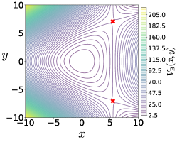
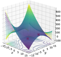
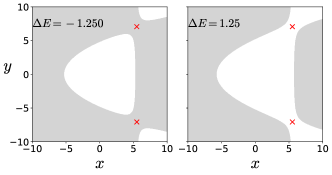
Figure 1: (a) Potential energy function underlying the coupled harmonic Hamiltonian (1) as isopotential contour and surface. The index-1 saddles are shown as red crosses in both the plots. (b) Hill’s region for energy below and above the energy of the index-1 saddle. Parameters used are $\omega_{x}=1.0,\omega_{y}=1.1,\delta=-0.11$.

Since this model system is conservative 2 DoF Hamiltonian, that is the phase space is $\mathbb{R}^{4}$, the energy surface is three dimensional, the dividing surface is two dimensional, and the normally hyperbolic invariant manifold (NHIM), referred to as the unstable periodic orbit, is one dimensional Wiggins (2016). Now, if we consider the intersection of a two dimensional surface with the three-dimensional energy surface, we would obtain the one-dimensional energy boundary on the surface of section. We will focus our study by using the isoenergetic two-dimensional surface

$$U_{xp_{x},+} =\left\{(x,y,p_{x},p_{y})\;|\;y=0,\;p_{y}(x,y,p_{x};e)>0\right\}$$ (3)

where the sign of the momentum coordinate enforces a directional crossing of the surface. Due to the form of the vector field (18) and choice of $\delta<0$, this directionality condition implies motion towards positive $y$-coordinate.

In this article, detecting the phase space structures will constitute finding the intersection of the NHIM and its invariant manifolds with a two dimensional surface (for example, Eqn. (3)).

II.2 Model system: coupled harmonic 3 DoF Hamiltonian

The next higher dimensional model system to consider is the coupled harmonic potential in 3 dimensions and underlying a 3 degrees-of-freedom system in Contopoulos et al. (1994); Farantos (1998). The Hamiltonian is given by

$$\begin{split}\mathcal{H}(x,y,z,p_{x},p_{y},p_{z})=T(p_{x},p_{y},p_{z})+V_{\rm BC}(x,y,z)\\ \mathrel{\phantom{=}}=\frac{1}{2}p_{x}^{2}+\frac{1}{2}p_{y}^{2}+\frac{1}{2}p_{z}^{2}+\\ \frac{1}{2}\omega_{x}^{2}x^{2}+\frac{1}{2}\omega_{y}^{2}y^{2}+\frac{1}{2}\omega_{z}^{2}z^{2}-\epsilon x^{2}y-\eta x^{2}z\end{split}$$ (4)

where $\omega_{x}^{2},\omega_{y}^{2},\omega_{z}^{2},\epsilon,\eta$ are the parameters related to the coupled harmonic 3 dimensional potential energy function Farantos (1998). In this study, we will fix the parameters to be $\omega_{x}^{2}=0.9,\omega_{y}^{2}=1.6,\omega_{z}^{2}=0.4,\epsilon=0.08,\eta=0.01$. The two index-1 saddle equilibria (as shown in the App. B) of the Hamiltonian vector field (68) are located at

$$\begin{split}\left(\pm\frac{\omega_{x}\omega_{y}\omega_{z}}{\sqrt{2(\epsilon^{2}\omega_{z}^{2}+\eta^{2}\omega_{y}^{2})}},\frac{\epsilon\omega_{x}^{2}\omega_{z}^{2}}{2(\epsilon^{2}\omega_{z}^{2}+\eta^{2}\omega_{y}^{2})},\right.\\ \left.\kern-1.2pt\frac{\eta\omega_{x}^{2}\omega_{y}^{2}}{2(\epsilon^{2}\omega_{z}^{2}+\eta^{2}\omega_{y}^{2})},0,0,0\right)\end{split}$$

and the total energy is

$$E_{c}=\frac{1}{8}\omega_{x}^{2}\frac{\omega_{x}^{2}\omega_{y}^{2}\omega_{z}^{2}}{\left(\epsilon^{2}\omega_{z}^{2}+\eta^{2}\omega_{y}^{2}\right)}.$$ (5)

The equilibrium point at $(0,0,0,0,0,0)$ is stable and has total energy $0$. For the parameters used in this study, the equilibrium points are located at $\left(\pm 10.290,5.294,2.647,0,0,0\right)$ and $\left(0,0,0,0,0,0\right)$ and have total energy, $E_{c}\approx 23.824$ and $E=0$, respectively.

We show the isopotential contours of the potential energy function at fixed value of $z_{\rm eq}$ in Fig. 2 along with the Hill’s regions for positive excess energy, $\Delta E=6.000$ and projected on the configuration space coordinates at the equilibrium point.

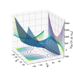
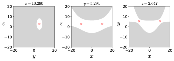
Figure 2: (a) Potential energy function underlying the coupled harmonic Hamiltonian (4) at $z_{\rm eq}=2.647$ as isopotential contour and surface. (b) Hill’s region for excess energy, $\Delta E=6.000$ and projected on the configuration space coordinates at the equilibrium point. We note here that the potential energy surface and the Hill’s region is plotted by fixing one of the configuration coordinates at the equilibrium point.

Since this model system is conservative 3 DoF Hamiltonian, that is the phase space is $\mathbb{R}^{6}$, the energy surface is five dimensional, the dividing surface is four dimensional, and the normally hyperbolic invariant manifold (NHIM) is three dimensional, or precisely 3-sphere, and its invariant manifolds are four dimensional, or precisely $\mathbb{R}^{1}\times\mathbb{S}^{3}$ or spherical cylinders Wiggins (2016). Now, if we consider the intersection of a two-dimensional section with the five dimensional energy surface in $\mathbb{R}^{6}$, we would obtain the one-dimensional energy boundary on the surface. We will focus our study near the bottleneck by considering the isoenergetic two dimensional surfaces

$$U_{xp_{x}}^{+}= \left\{(x,y,z,p_{x},p_{y},p_{z})\;|\;y=y_{\rm eq},z=z_{\rm eq},\;p_{y}=0,\;p_{z}(x,y,z,p_{x},p_{y};e)>0\right\}$$ (6)

$$U_{yp_{y}}^{+}= \left\{(x,y,z,p_{x},p_{y},p_{z})\;|\;x=x_{\rm eq},z=z_{\rm eq},\;p_{x}=0,\;p_{z}(x,y,z,p_{x},p_{y};e)>0\right\}$$ (7)

$$U_{zp_{z}}^{+}= \left\{(x,y,z,p_{x},p_{y},p_{z})\;|\;x=x_{\rm eq},y=y_{\rm eq},\;p_{x}=0,\;p_{y}(x,y,z,p_{x},p_{z};e)>0\right\}$$ (8)

In this 3 DoF system, detecting points on the three dimensional NHIM and four dimensional invariant manifolds will constitute finding their intersection with the above two dimensional surfaces.

II.3 Method: Lagrangian descriptor

The Lagrangian descriptor (LD) as presented in Ref.Madrid and Mancho (2009) is the arc length of a trajectory calculated on a chosen initial time $t_{0}$ and measured for fixed forward and backward integration time, $\tau$. For continuous time dynamical systems, Ref.Lopesino et al. (2017) gives an alternative definition of the LD which is useful for proving rigorous results and can be computed along with the trajectory. It provides a characterization of the notion of singular features of the LD that facilitates a proof for detecting invariant manifolds in certain model situations. In addition, the “additive nature” of this new definition of LD provides an approach for assessing the influence of each degree-of-freedom separately. This property was used in Ref.Demian and Wiggins (2017) to show that Lagrangian descriptor can detect Lyapunov periodic orbits in the two degrees-of-freedom Hénon-Heiles system. We will adopt a similar strategy for the aforementioned two and three degrees-of-freedom autonomous Hénon-Heiles type systems.

In the general setting of a time-dependent vector field

$$\frac{d\mathbf{x}}{dt}=\mathbf{v}(\mathbf{x},t),\quad\mathbf{x}\in\mathbb{R}^{n}\;,\;t\in\mathbb{R}$$ (9)

where $\mathbf{v}(\mathbf{x},t)\in C^{r}$ ($r\geq 1$) in $\mathbf{x}$ and continuous in time. The definition of LDs depends on the initial condition $\mathbf{x}_{0}=\mathbf{x}(t_{0})$, on the initial time $t_{0}$ (trivial for autonomous systems) and the integration time $\tau$, and the type of norm of the trajectory’s components, and takes the form,

$$M_{p}(\mathbf{x}_{0},t_{0},\tau)=\displaystyle{\int^{t_{0}+\tau}_{t_{0}-\tau}\sum_{i=1}^{n}|\dot{x}_{i}(t;\mathbf{x}_{0})|^{p}\;dt}$$ (10)

where $p\in(0,1]$ and $\tau\in\mathbb{R}^{+}$ are freely chosen parameters, and the overdot symbol represents the derivative with respect to time. It is to be noted here that there are three formulations of the function $M_{p}$ in the literature: the arc length of a trajectory in phase space Madrid and Mancho (2009), the arc length of a trajectory projected on the configuration space  Junginger et al. (2016); Junginger and Hernandez (2016b); Junginger et al. (2017a, b), and the sum of the $p$-norm of the vector field components Lopesino et al. (2015, 2017). Although the latter formulation of the Lagrangian descriptor (10) developed in Ref. Lopesino et al. (2015, 2017) does not resemble the arc length, the numerical results using either of these forms have been shown to be in agreement and promise of predictive capability in geophysical flows de la Cámara et al. (2012); Mendoza, Mancho, and Wiggins (2014); García-Garrido, Mancho, and Wiggins (2015); Ramos et al. (2018). The formulation we adopt here is motivated by the fact that this allows for proving rigorous result, which we will discuss in the next section, connecting the singular features and minimum in the LD plots with NHIM and its stable and unstable manifolds. It follows from the result that

$$\mathcal{W}^{s}(\mathbf{x}_{0},t_{0}) =\text{\rm argmin}\;\mathcal{L}^{(f)}(\mathbf{x}_{0},t_{0},\tau)$$ (11)

$$\mathcal{W}^{u}(\mathbf{x}_{0},t_{0}) =\text{\rm argmin}\;\mathcal{L}^{(b)}(\mathbf{x}_{0},t_{0},\tau)$$ (12)

where the stable and unstable manifolds ($\mathcal{W}^{s}(\mathbf{x}_{0},t_{0})$ and $\mathcal{W}^{u}(\mathbf{x}_{0},t_{0})$) denote the invariant manifolds at intial time $t_{0}$ and $\text{\rm argmin}\;(\cdot)$ denotes the argument that minimizes the function $\mathcal{L}^{(\cdot)}(\mathbf{x}_{0},t_{0},\tau)$ in forward and backward time, respectively. In addition, the coordinates on the NHIM, $\mathcal{M}(\mathbf{x}_{0},t_{0})$ at time $t_{0}$ is given by the intersection $\mathcal{W}^{s}(\mathbf{x}_{0},t_{0})$ and $\mathcal{W}^{u}(\mathbf{x}_{0},t_{0})$ of the stable and unstable manifolds, and thus given by

$$\mathcal{M}(\mathbf{x}_{0},t_{0}) =\text{\rm argmin}\;\left(\mathcal{L}^{(f)}(\mathbf{x}_{0},t_{0},\tau)+\mathcal{L}^{(b)}(\mathbf{x}_{0},t_{0},\tau)\right)$$ (13)

$$=\text{\rm argmin}\;\mathcal{L}(\mathbf{x}_{0},t_{0},\tau)$$

In applying the LD method to nonlinear systems, one observes multiple minima and singularities that can lead to trouble with isolating the one minima due to the NHIM and the ones due to its invariant manifolds. Since, as we integrate initial conditions on an isoenergetic two dimensional surface such as $U_{xp_{x}}^{+}$ (3), almost all trajectories that escape to infinity get integrated for the entire time interval and result in numerical overflow of the function M value (10) and show up as NaN. This can, however, be avoided by integrating for shorter time interval but this will vary for different locations of a surface. Thus, leading to trouble in locating the point with minimum and singularity in LD contour map that correspond to NHIM and its invariant manifolds.

This computational issue has been addressed in recent efforts to locate transition state trajectory in driven and 3 degrees-of-freedom chemical reaction dynamics Craven, Junginger, and Hernandez (2017); Craven and Hernandez (2016, 2015). It has been noted that computing fixed integration time Lagrangian descriptor (LD) leads to two potential issues:

1. Bounded trajectories will show global recrossings of the barrier as predicted by Poincaré recurrrence theorem. The recrossings will show multiple minima and singularities (as in Fig. 3(d-f)) in the LD plot which obscures locating the actual NHIM.

2. The trajectories that escape the potential well will leave with ever increasing acceleration, if the potential energy surface opens out to infinity. The trajectories with NaN LD values will render the contour map flat which again obscures locating the NHIM.

To circumvent these issues, a heuristic that has been adopted in the literature is to calculate LD values only until a trajectory remains inside the barrier region. The immediate result is the initial condition on an invariant manifold will have a maxima in the LD values because of being integrated for the full integration time (preselected) interval.

Thus, the formulation (10) is modified as

$$M_{p}(\mathbf{x}_{0},t_{0},\tau^{\pm})=\displaystyle{\int^{t_{0}+\tau^{+}}_{t_{0}-\tau^{-}}\sum_{i=1}^{n}|\dot{x}_{i}(t;\mathbf{x}_{0})|^{p}\;dt}$$ (14)

where the integration time interval depends on a trajectory and given by

$$\tau^{\pm}(\mathbf{x}_{0})=\min\left(\tau,t|_{|\mathbf{x}(t)|>q_{s}}\right)$$ (15)

where $q_{s}$ defines a domain, called the saddle region, in the configuration space around the saddle. We note here that the only initial condition that gets integrated for the entrire $\tau$ time units in forward and backward time is the one on the NHIM. In addition, the coordinates on the NHIM, $\mathcal{M}(\mathbf{x}_{0},t_{0})$, at time $t_{0}$ is given by

$$\mathcal{M}(\mathbf{x}_{0},t_{0}) =\text{\rm argmax}\;\left(\mathcal{L}^{(f)}(\mathbf{x}_{0},t_{0},\tau)+\mathcal{L}^{(b)}(\mathbf{x}_{0},t_{0},\tau)\right)$$ (16)

$$=\text{\rm argmax}\;\mathcal{L}(\mathbf{x}_{0},t_{0},\tau)$$

This is also a familiar from a dynamical systems perspective where the literature on average exit times to locate invariant sets has been discussed for the symplectic maps (see Meiss (1997) and related references). However, the connection between features in exit times and LD contour maps is not the focus of this study and will be deferred as related future work.

III Results

We begin by noting that two-dimensional Poincaré surface of section have sufficient dimensionality to capture trajectories on a three dimensional energy surface, however for high dimensional systems trajectories can go “around” the two dimensional surface. One approach available in the literature is to use high dimensional Poincaré sections which can “catch” trajectories but are hard to visualize on paper or in the virtual 3D space. Even when gets around this issue, using suitable projective geometry, the fact that the qualitative analysis based on Poincaré sections depends on trajectories returning to this surface can not be circumvented since trajectories on and inside the spherical cylinders will not return to the Poincaré surface of section.

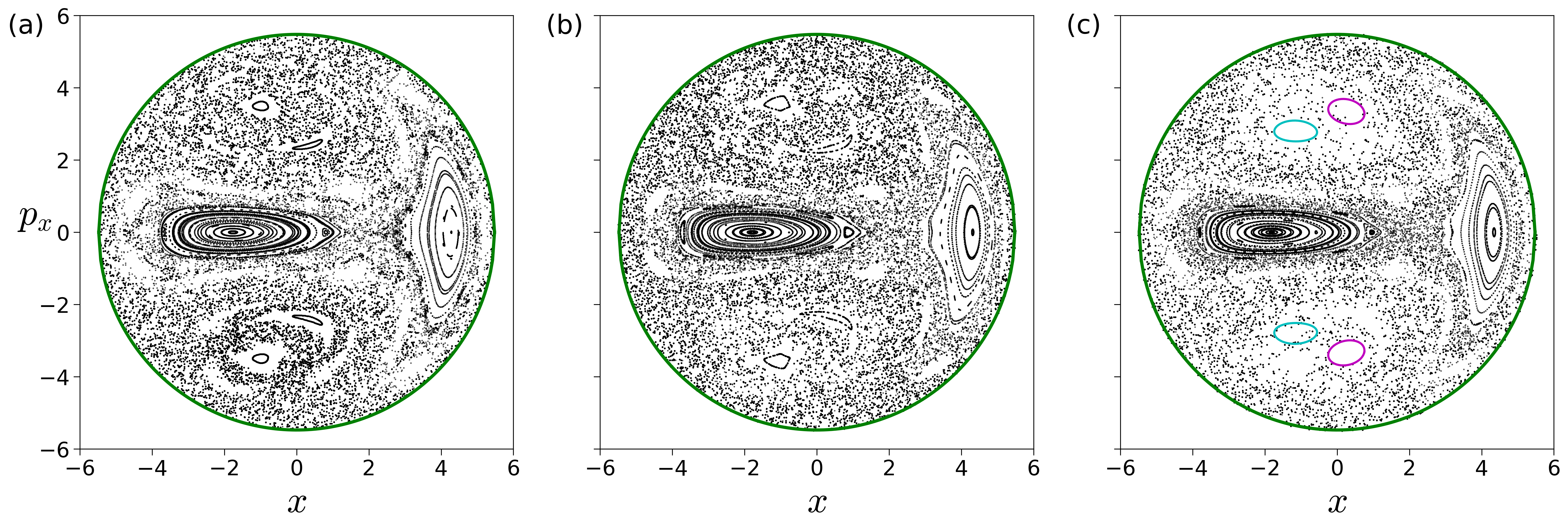
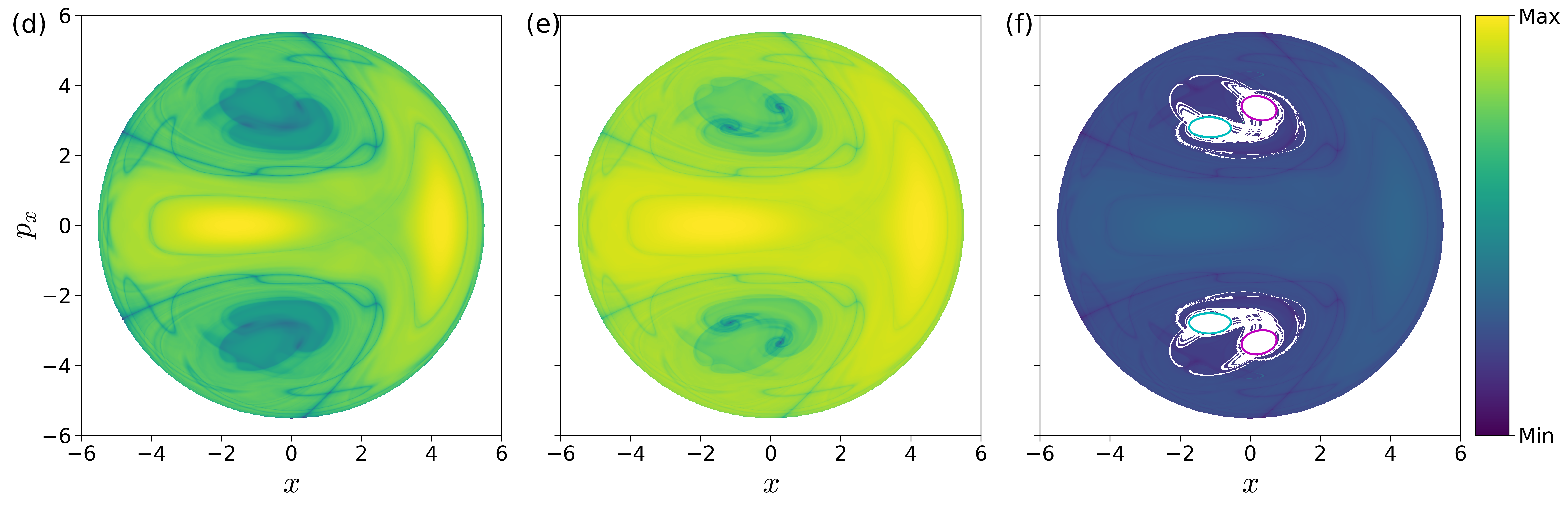
Figure 3: Top row: Poincaré surface of section, $U_{xp_{x}}$ (3), at excess energy (a) $\Delta E=-0.125$, (b) $\Delta E=0.000$, (c) $\Delta E=0.125$ where the intersection of the surface of section with the energy surface is shown in green. Bottom row: Lagrangian descriptor on the surface of section, $U_{xp_{x}}$ (3), for the excess energies (d) $\Delta E=-0.125$, (e) $\Delta E=0.000$, (f) $\Delta E=0.125$ and the integration time $\tau=50$. The intersection of the surface of section with the cylindrical manifolds of the NHIM —unstable periodic orbit for this system —associated with the index-1 saddle equilibrium point in the bottleneck is shown in cyan (stable) and magenta (unstable) curves. The magenta and cyan curves in $p_{x}>0$ correspond to the invariant manifolds of unstable periodic orbit at $y>0$ index-1 saddle, and the ones in $p_{x}<0$ correspnd to the invariant manifolds of unstable periodic orbit at $y<0$ index-1 saddle.

III.1 Coupled harmonic 2 DoF system

As discussed in aforementioned literature Madrid and Mancho (2009); Lopesino et al. (2017); Demian and Wiggins (2017), points with minimum Lagrangian descriptor (LD) values and singularity are on the invariant manifolds. In addition, LD plots show dynamical correspondence with Poincaré sections (in the sense that regions with regular and chaotic dynamics are distinct in both Poincaré section and LD plots) while also depicting the geometry of manifold intersections Demian and Wiggins (2017); Lopesino et al. (2017); García-Garrido et al. (2018). This correspondence in the LD features and Poincaré section is confirmed in Fig. 3 where we show the Poincaré surface of section Eqn. (3) of trajectories and LD contour maps on the same isoenergetic two-dimensional surface for negative and positive excess energies. It can be seen that the chaotic dynamics as marked by the sea of points in Poincaré section is revealed as the tangle of invariant manifolds which are points of minima and singularity in the LD plots. As shown by the one dimensional slices of the LD plots, there are multiple such minima and singularities and as the excess energy is increased to positive values, there are regions of discontinuities along the one dimensional slice. Next, as the energy is increased and the bottleneck opens at critical energy $E_{c}$, trajectories that leave the potential well and do not return to the surface of section are not observed on the Poincaré section while the LD contour maps clearly identifies these regions as discontinuities in the LD values. These regions lead to escape because they are inside the cylindrical manifolds of the unstable periodic orbit associated with the index-1 saddle equilibrium point Naik and Ross (2017). These regions on the isoenergetic two-dimensional surface are also referred to as reactive islands in chemical reaction dynamics De Leon (1992); De Leon, Mehta, and Topper (1991a, b). The escape regions or reactive islands that appear over the integration time interval can also be identified by using the forward and backward LD contour maps where these regions appear as discontinuities. In Fig. 3(f), we show these for $\Delta E=0.125$ and $\tau=50$ along with the intersection of the cylindrical manifolds’ intersections that are computed using differential correction and numerical continuation. The detailed comparison and extension to high dimensional systems is not the focus of this study and will be discussed in forthcoming work. Thus LD maps also provide a quick and reliable approach for detecting regions that will lead to escape within the observed time, or in the computational context, the integration time.

To detect the NHIM — in this case, unstable periodic orbit — associated with the index-1 saddles (marked by cross in Fig. 1), we define an isoenergetic two dimensional surface that is parametrized by the $y$-coordinate and placed near the $x$-coordinate of the saddle equilibrium that has the negative $y$-coordinate. This can be expressed as a parametric two dimensional surface

$$U_{xp_{x}}^{+}(k)= \left\{(x,y,p_{x},p_{y})\,|\,y=k,p_{y}(x,y,p_{x};e)>0\right\}$$ (17)

for total energy, $e$, which is above the critical energy, $E_{c}$, $k$ is the $y$-coordinate. The variable integration time LD contour maps are shown in Fig. 4 along with the projection of the low dimensional slices (17) in the configuration space and the NHIM. The points on NHIM, which is an unstable periodic orbit for 2 DoF, on this surface is the coordinate with maximum (for variable integration time) LD value. The full visualization of the NHIM as the black ellipse, $\mathbb{S}^{1}$, is in Fig. 4(d) and has been computed using differential correction and numerical continuation (details in App. A.1) and shows clearly that points on this unstable periodic orbit are detected by the LD contour map.

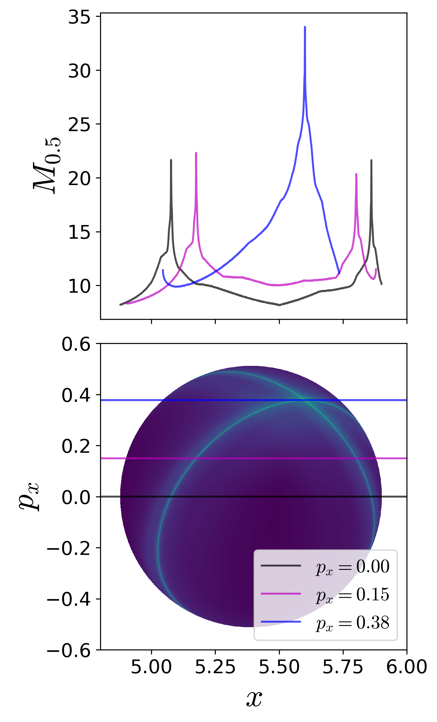
(a) $U_{xp_{x}}^{+}(-7.0)$

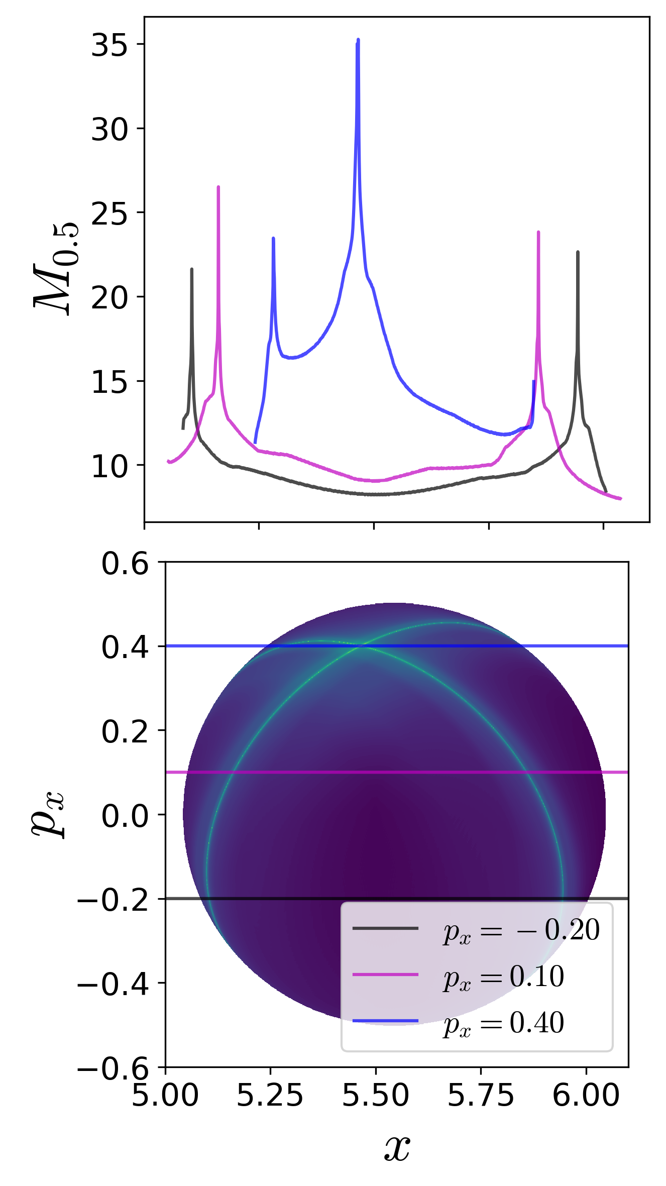
(b) $U_{xp_{x}}^{+}(-7.1)$

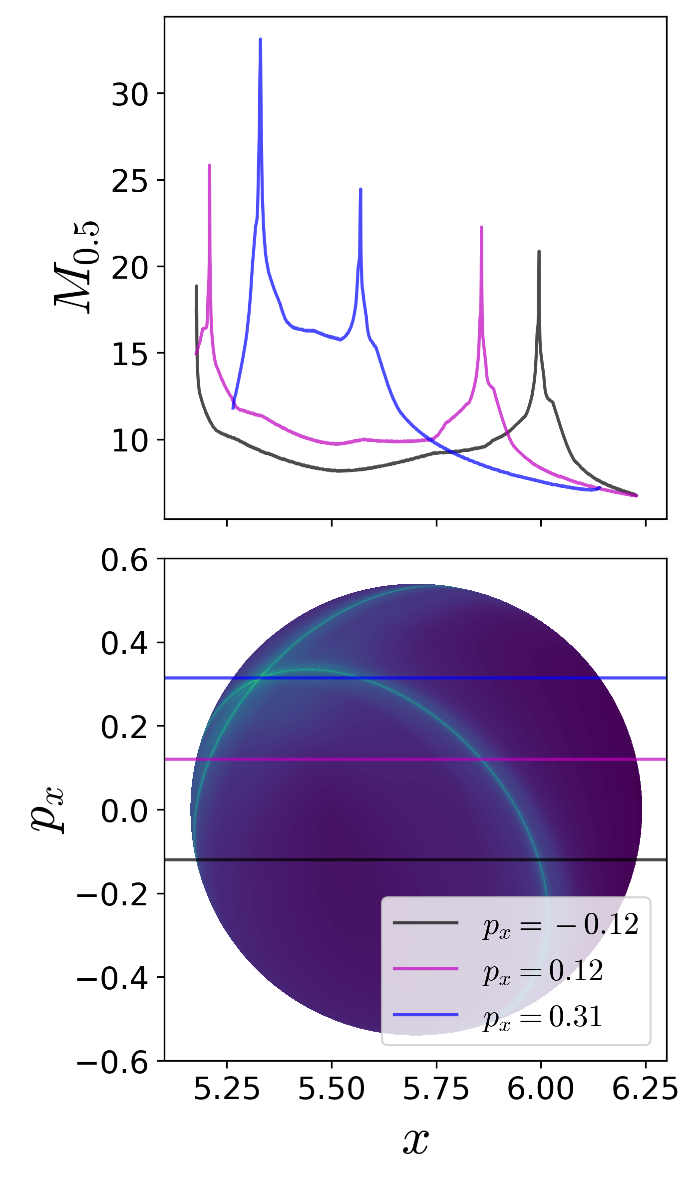
(c) $U_{xp_{x}}^{+}(-7.2)$

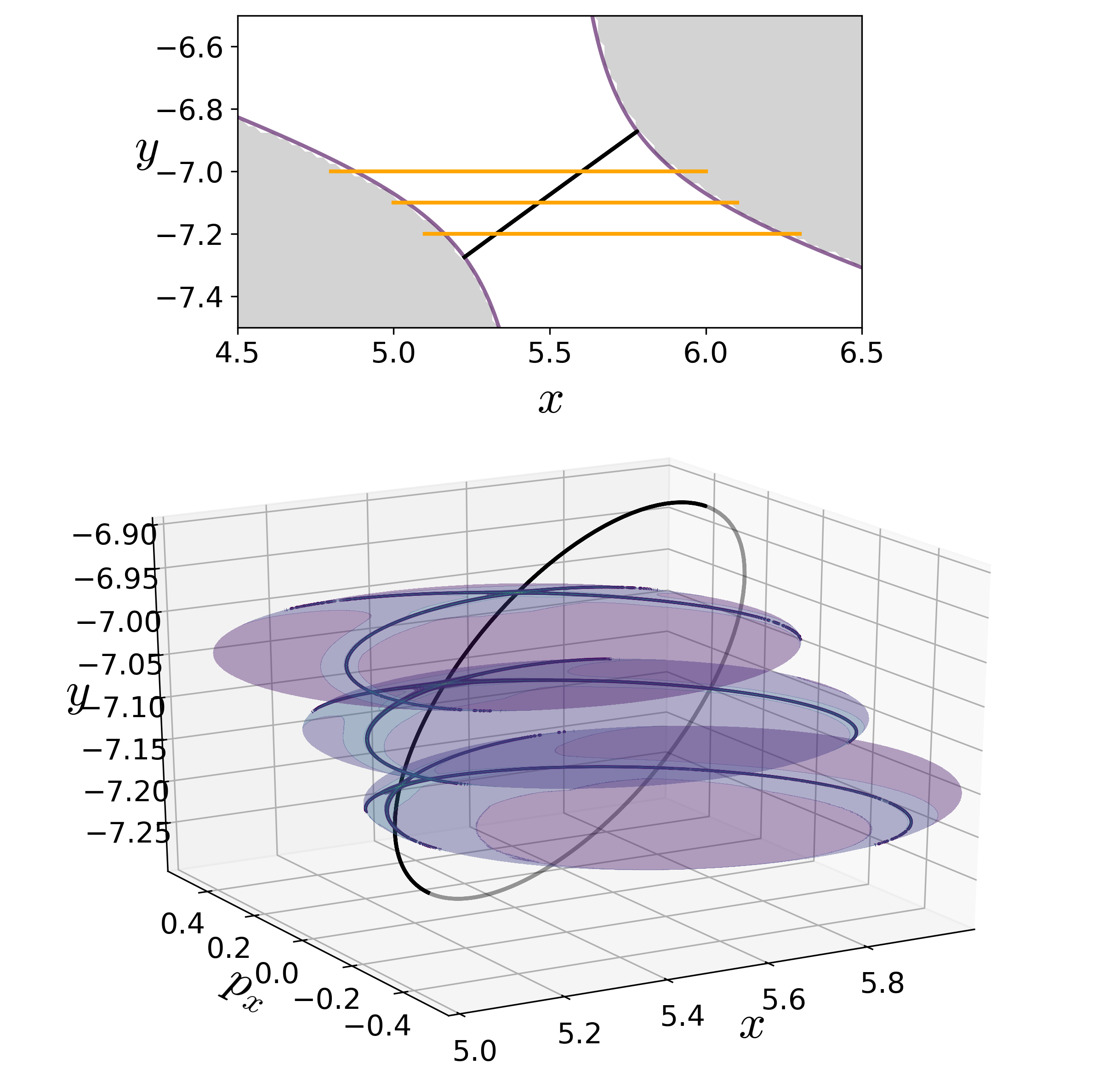
Figure 4: Lagrangian descriptor computed for variable integration time on two dimensional slices (17) near the bottleneck that detect the NHIM and its invariant manifolds associated with the index-1 saddle. The two dimensional surfaces are shown in the top figure in (d) projected as orange lines on the configuration space and the unstable periodic orbit as black line connecting the isopotential contour corresponding to $\Delta E=0.125$ with the Hill’s region shown in grey. The two dimensional slices represent low dimensional probe of the unstable periodic orbit and the movie of a rotating view can be found here.

III.2 Coupled harmonic 3 DoF system

The Lagrangian descriptor based approach for detecting NHIM in 2 DoF system can now be applied to the 3 DoF system (4). On the five dimensional energy surface, the phase space structures such as the NHIM and its invariant manifolds are three and four dimensional, respectively Wiggins (2016). As noted earlier, direct visualization techniques will fall short in 4 or more DoF systems even if they are successful in 2 and 3 DoF. So, LD based approach can be used to detect points on a NHIM and its invariant manifolds using low dimensional probe which are based on trajectory diagnostic on an isoenergetic two dimensional surface.

It is to be noted that the increase in phase space dimension, leads to a polynomial scaling in the number of coordinate pairs (that is $2N(2N-1)(N-1)$ coordinate pairs for $N$ DoF system) and is thus, impractical to present the procedure on all the combination of coordinates. We will present the results for the three configuration space coordinates by combining each with its corresponding momentum coordinate.

On these isoenergetic surfaces, we compute the variable integration time Lagrangian descriptor for small excess energy, $\Delta E\approx 0.176$, or total energy $E=24.000$, and show the contour maps in Fig. 5. The maxima identifying the points on the NHIM and its invariant manifolds can be visualized using one dimensional slices for constant momenta. This indicates clearly the initial conditions in the phase space (points on the isoenergetic two dimensional surfaces in $\mathbb{R}^{6}$, for example (6)) that do not leave the saddle region.

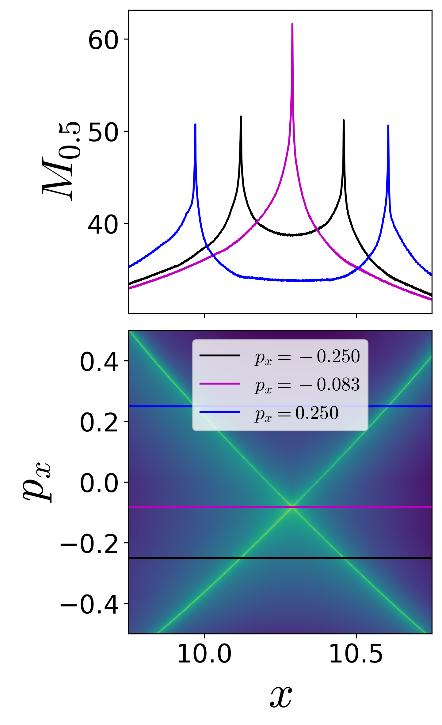
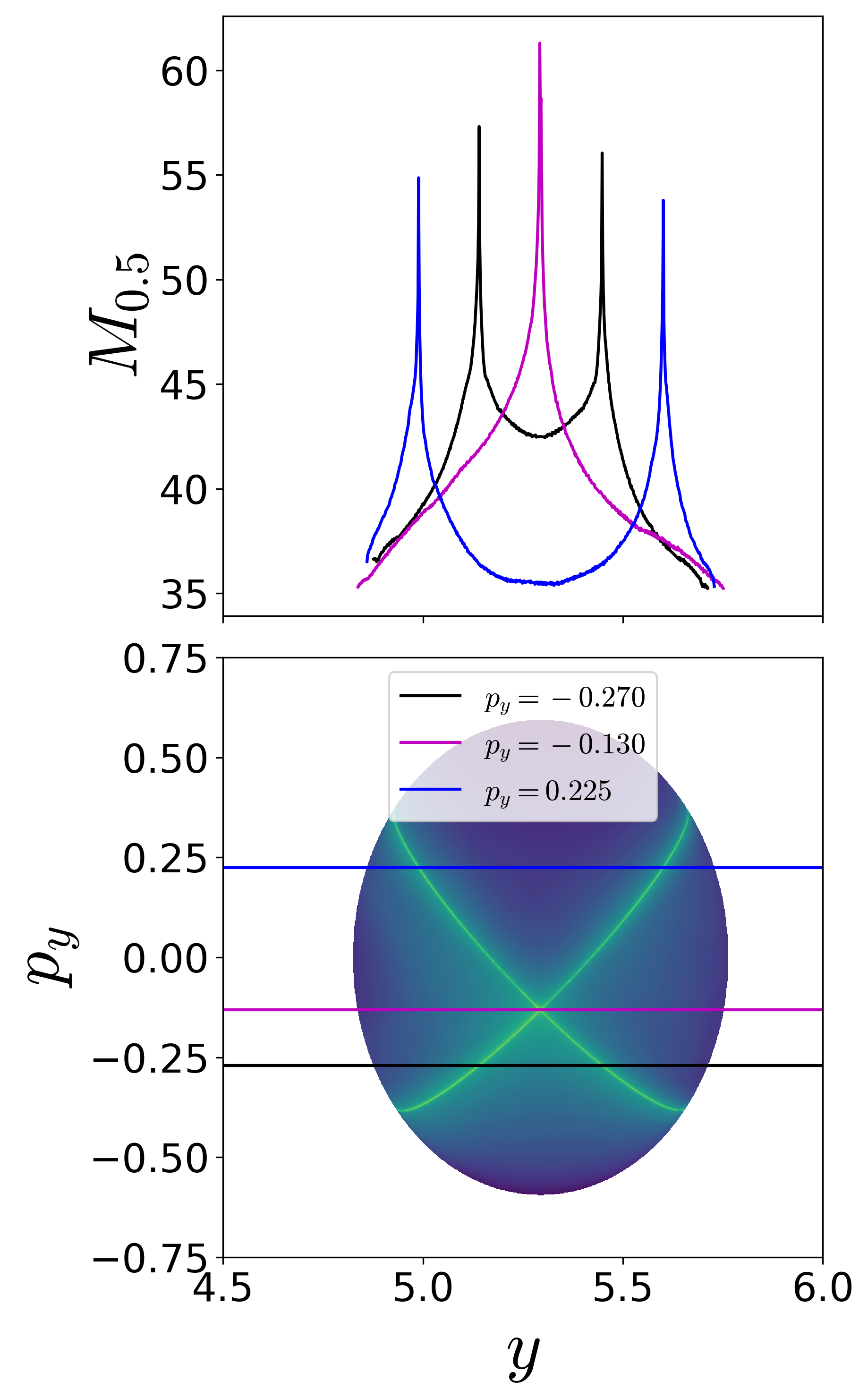
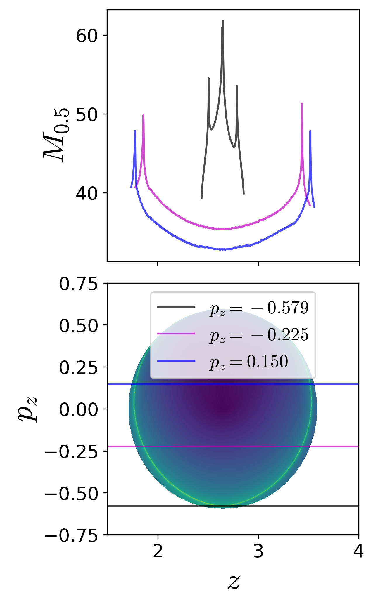
Figure 5: Detecting points on the NHIM using variable integration time Lagrangian descriptor on the two dimensional surfaces (a) $U_{xp_{x}}^{+}$ (6), (b) $U_{yp_{y}}^{+}$ (7), and (c) $U_{zp_{z}}^{+}$ (8) at excess energy $\Delta E\approx 0.176$ or total energy $E=24.000$. For this energy value, the saddle region, as defined in Eqn. (15), is taken to be $q_{s}=[9,12]\times[2.5,7.5]\times[1,4]$ and $\tau=50$.

IV Conclusions

In this article, we discussed a trajectory diagnostic method as a low dimensional probe of high dimensional invariant manifolds in 2 and 3 DoF nonlinear Hamiltonian systems. This trajectory diagnostic — Lagrangian descriptor (LD) — can represent a geometric property of interest in a system with escape/transition and features, that is minima or maxima, in its contour map identify points on the high dimensional invariant manifolds.

Comparing the points on the NHIM in 2 DoF system obtained using the LD method with differential correction and numerical continuation, we also verified the method for a nonlinear autonomous system following our previous work on decoupled and coupled 2 and 3 DoF linear system Naik, García-Garrido, and Wiggins (2019). The results on 3 DoF system are also congruent with what one expects for an extended problem of the 2 DoF coupled harmonic potential. In addition, the LD method based detection of NHIM is simple to implement and quickly provides a lay of the dynamical land which is a preliminirary step in applying phase space transport to problems in physics and chemistry. This method can also be used to set up starting guess for other numerical procedures which rely on good initial guess or can also be used in conjunction with machine learning methods for rendering the smooth pieces of NHIM Bardakcioglu et al. (2018); Feldmaier et al. (2019).

Appendix A Coupled harmonic 2 DoF system

For this system, Hamilton’s equations of motion are

$$\dot{x} =p_{x}$$ (18)

$$\dot{y} =p_{y}$$

$$\dot{p}_{x} =-\frac{\partial V}{\partial x}=-(\omega_{x}^{2}x+\delta y^{2})$$

$$\dot{p}_{y} =-\frac{\partial V}{\partial y}=-(\omega_{y}^{2}y+2\delta xy)$$

Hill’s region and zero velocity curve — The projection of energy surface into configuration space, $(x,y)$ plane, is the region of energetically possible motion for an energy $E(x,y,p_{x},p_{y})=e$. Let $M(e)$ denote this projection defined as

$$M(e)=\left\{(x,y)\,|\,V_{B}(x,y)\leqslant e\right\}$$ (19)

where $V_{B}(x,y)$ is the potential energy function (1). The projection (19) of energy surface is known in mechanics as the Hill’s region. The boundary of $M(e)$ is known as the zero velocity curve, and plays an important role in placing bounds on the motion of a phase space point for a given total energy. The zero velocity curves are the locus of points in the $(x,y)$ plane where the kinetic energy, and hence the angular velocity vector vanishes, that is

$$E(x,y,p_{x},p_{y})=e= \frac{1}{2}\left(p_{x}^{2}+p_{y}^{2}\right)+V_{B}(x,y)$$ (20)

$$p_{x}^{2}+p_{y}^{2}= 2(e-V_{B}(x,y))=0$$ (21)

From Eqn. (19), it is clear that the state is only able to move on the side of this curve for which the kinetic energy is positive. The other side of the curve, where the kinetic energy is negative and motion is impossible, is referred to as the energetically forbidden realm, and shown as gray region.

Symmetries of the equations of motion — We note the symmetries in the system (18), by substituting $(-y,-p_{y})$ for $(y,p_{y})$ which implies reflection about the $x-$axis and expressed as

$$s_{y}:(x,y,p_{x},p_{y},t)\rightarrow(x,-y,p_{x},-p_{y},t)$$ (22)

Thus, if $(x(t),y(t),v_{x}(t),v_{y}(t))$ is a solution to (18), then $(x(t),-y(t),p_{x}(t),-p_{y}(t))$ is another solution. The conservative system also has time-reversal symmetry

$$s_{t}:(x,y,p_{x},p_{y},t)\rightarrow(x,y,-p_{x},-p_{y},-t)$$ (23)

So, if $(x(t),y(t),p_{x}(t),p_{y}(t))$ is a solution to (18), then $(x(-t),y(-t),-p_{x}(-t),-p_{y}(-t))$ is another solution. These symmetries can be used to decrease the number of computations, and to find special solutions. For example, any solution of (18) will evolve on the energy surface given by (1). For fixed energy, $E(x,y,p_{x},p_{y})=e$, there will be zero velocity curves corresponding to $V_{B}(x,y)=e$, the contours shown in Fig. 1. Any trajectory which touches the zero velocity curve at time $t_{0}$ must retrace its path in configuration space (i.e., $q=(x,y)$ space),

$$q(-t+t_{0})=q(t+t_{0})\qquad\mathring{q}(-t+t_{0})=-\mathring{q}(t+t_{0})$$ (24)

A.1 Computing the NHIM and its invariant manifolds associated with the index-1 saddle

For the ease with discussing the geometry, we call the equilibrium with positive y-coordinate $\mathbf{x}_{\rm eq,top}$ and negative y-coordinate $\mathbf{x}_{\rm eq,bot}$.

Select appropriate energy above the critical value —  For computation of manifolds that act as boundary between the transition and non-transition trajectories, we select the total energy, $E$, above the critical value and so the excess energy $\Delta E>0$. This excess energy can be arbitrarily large as long as the energy surface stays within the dynamical system’s phase space bounds.

Differential correction and numerical continuation for the NHIM —  We consider a procedure which computes periodic orbits around in a relatively straightforward fashion. This procedure begins with small “seed” initial conditions obtained from the linearized equations of motion near $\mathbf{x}_{\rm eq,bot}$ and uses differential correction and numerical continuation to generate the desired periodic orbit corresponding to the chosen energy $E$ (Koon et al. (2011)). The result is a periodic orbit of the desired energy $E$ of some period $T$, which will be close to $2\pi/\omega$ where $\pm i\omega$ is the imaginary pair of eigenvalues of the linearization around the saddle point.

Guess initial condition of the periodic orbit — The linearized equations of motion near an equilibrium point can be used to initialize a guess for the differential correction method. Let us select the equilibrium point, $\mathbf{x}_{\rm eq,bot}$. The linearization yields an eigenvalue problem $Av=\gamma v$, where $A$ is the Jacobian matrix (50) evaluated at the equilibrium point, $\gamma$ is the eigenvalue, and $v=[k_{1},k_{2},k_{3},k_{4}]^{T}$ is the corresponding eigenvector. Thus, using the structure of $A$ from Eqn. (50) we can write

$$k_{3} =\gamma k_{1}$$ (25)

$$k_{4} =\gamma k_{2}$$

$$ak_{1}+bk_{2} =\gamma k_{3}$$

$$ck_{1}+dk_{2} =\gamma k_{4}$$

where $a,b,c,d$ are entries in the Jacobian (50) and evaluated at the equilibrium point $(x_{\rm eq,bot},y_{\rm eq,bot},0,0)$. So when $\gamma=\pm\lambda$, which correspond to the saddle directions of the equilibrium point, the corresponding eigenvectors are

$$u_{1} =[1,k_{2},\lambda,\lambda k_{2}]$$ (26)

$$u_{2} =[1,k_{2},-\lambda,-\lambda k_{2}]$$

and when $\gamma=\pm i\omega$, which correspond to the center directions, the corresponding eigenvectors are

$$w_{1} =[1,k_{2},i\omega,i\omega k_{2}]$$ (27)

$$w_{2} =[1,k_{2},-i\omega,-i\omega k_{2}]$$

where, $k_{2}=(\gamma^{2}-a)/b$ is the constant depending on the eigenvalue, $\gamma$. Thus, the general solution of linearized equation of motion in Eqn. (67) can be used to initialize a guess for the periodic orbit for a small amplitude, $A_{x}\approx 10^{-4}$. The idea is to use the complex eigenvalue and the corresponding eigenvector to obtain a starting guess for the initial condition on the periodic orbit and its period $T_{\rm po}$, which should be close to $2\pi/\omega$ (generalization of Liapounov’s theorem) and increase monotonically with excess energy, $\Delta E$.

The initial condition for a periodic orbit of x-amplitude, $A_{x}>0$ can be computed by letting $A_{1}=A_{2}=0$ and $t=0$ in Eqn. (67), and $\beta=-A_{x}/2$ (this choice is made to get rid of factor 2) denotes a small amplitude in the general linear solution. Thus, using the eigenvector along the center direction we can guess the initial condition to be

$$\bar{\mathbf{x}}_{\rm 0,g}= \begin{pmatrix}x_{\rm eq,bot},y_{\rm eq,bot},0,0\end{pmatrix}^{T}+2Re(\beta w_{1})$$ (28)

$$= \begin{pmatrix}x_{\rm eq,bot}-A_{x},y_{\rm eq,bot}-A_{x}k_{2},0,0\end{pmatrix}^{T}$$

Without loss of generality, let us consider the bottom index-1 saddle equilibrium point (on the potential energy surface, $y<0$), then the initial guess is given by

$$\bar{\mathbf{x}}_{0,\rm g}= \left(-\frac{\omega_{y}^{2}}{2\delta},-\frac{1}{\sqrt{2}}\frac{\omega_{x}\omega_{y}}{\delta},0,0\right)+$$ (29)

$$\left(A_{x},\frac{A_{x}(\omega^{2}-\omega_{x}^{2})}{\sqrt{2}\omega_{x}\omega_{y}},0,0\right)$$

Differential correction of the initial condition — In this procedure, we attempt to introduce small change in the initial guess such that the periodic orbit $\bar{\mathbf{x}}_{\rm po}$

$$\left\|\bar{\mathbf{x}}_{\rm po}(T)-\bar{\mathbf{x}}_{\rm po}(0)\right\|<\epsilon$$ (30)

for some tolerance $\epsilon<<1$. In this approach, we hold $x-$coordinate constant, while applying correction to the initial guess of the $y-$coordinate, use $v_{y}-$coordinate for terminating event-based integration, and $v_{x}-$coordinate to test convergence of the periodic orbit. It is to be noted that this combination of coordinates is suitable for the structure of initial guess at hand, and in general will require some permutation of the phase space coordinates to achieve a stable algorithm.

Let us denote the flow map of a differential equation $\mathring{\mathbf{x}}=\mathbf{f}(\mathbf{x})$ with initial condition $\mathbf{x}(t_{0})=\mathbf{x}_{0}$ by $\phi(t;\mathbf{x}_{0})$. Thus, the displacement of the final state under a perturbation $\delta t$ becomes

$$\delta\bar{\mathbf{x}}(t+\delta t)=\phi(t+\delta t;\bar{\mathbf{x}}_{0}+\delta\bar{\mathbf{x}}_{0})-\phi(t;\bar{\mathbf{x}}_{0})$$ (31)

with respect to the reference orbit $\bar{\mathbf{x}}(t)$. Thus, measuring the displacement at $t_{1}+\delta t_{1}$ and expanding into Taylor series gives

$$\delta\bar{\mathbf{x}}(t_{1}+\delta t_{1})=\frac{\partial\phi(t_{1};\bar{\mathbf{x}}_{0})}{\partial\mathbf{x}_{0}}\delta\bar{\mathbf{x}}_{0}+\frac{\partial\phi(t_{1};\bar{\mathbf{x}}_{0})}{\partial t_{1}}\delta t_{1}+h.o.t$$ (32)

where the first term on the right hand side is the state transition matrix, $\mathbf{\Phi}(t_{1},t_{0})$, when $\delta t_{1}=0$. Thus, it can be obtained as numerical solution to the variational equations as discussed in Parker and Chua (1989). Let us suppose we want to reach the desired point $\mathbf{x}_{\rm d}$, we have

$$\bar{\mathbf{x}}(t_{1})=\phi(t_{1};\bar{\mathbf{x}}_{0})=\bar{\mathbf{x}}_{1}=\mathbf{x}_{d}-\delta\bar{\mathbf{x}}_{1}$$ (33)

which has an error $\delta\bar{\mathbf{x}}_{1}$ and needs correction. This correction to the first order can be obtained from the state transition matrix at $t_{1}$ and an iterative procedure of this small correction based on first order yields convergence in few steps. For the equilibrium point under consideration, we initialize the guess as

$$\bar{\mathbf{x}}(0)=(x_{0,g},y_{0,g},0,0)^{T}$$ (34)

and using numerical integrator we continue until next $v_{x}=0$ event crossing with a high pecified tolerance (typically $10^{-14}$). So, we obtain $\bar{\mathbf{x}}(t_{1})$ which for the guess periodic orbit denotes the half-period point, $t_{1}=T_{0,g}/2$ and compute the state transition matrix $\mathbf{\Phi}(t_{1},0)$. This can be used to correct the initial value of $y_{0,g}$ to approximate the periodic orbit while keeping $x_{0,g}$ constant. Thus, correction to the first order is given by

$$\delta v_{x_{1}}=\Phi_{32}\delta y_{0}+\mathring{v}_{x_{1}}\delta t_{1}+h.o.t$$ (35)

$$\delta v_{y_{1}}=\Phi_{42}\delta y_{0}+\mathring{v}_{y_{1}}\delta t_{1}+h.o.t$$ (36)

where $\Phi_{ij}$ is the $(i,j)^{th}$ entry of $\mathbf{\Phi}(t_{1},0)$ and the acceleration terms come from the equations of motion evaluated at the crossing $t=t_{1}$ when $v_{x_{1}}=\delta v_{x_{1}}=0$. Thus, we obtain the first order correction $\delta y_{0}$ as

$$\delta y_{0} \approx\left(\Phi_{42}-\Phi_{32}\frac{\mathring{v}_{y_{1}}}{\mathring{v}_{x_{1}}}\right)^{-1}\delta v_{y_{1}}$$ (37)

$$y_{0} \rightarrow y_{0}-\delta y_{0}$$ (38)

which is iterated until $|v_{y_{1}}|=|\delta v_{y_{1}}|<\epsilon$ for some tolerance $\epsilon$, since we want the final periodic orbit to be of the form

$$\bar{\mathbf{x}}_{t_{1}}=(x_{1},y_{1},0,0)^{T}$$ (39)

This procedure yields an accurate initial condition for a periodic orbit of small amplitude $A_{x}<<1$, since our initial guess is based on the linear approximation near the equilibrium point. It is also to be noted that differential correction assumes the guess periodic orbit has a small error (for example in this system, of the order of $10^{-2}$) and can be corrected using first order form of the correction terms. If, however, larger steps in correction are applied this can lead to unstable convergence as the half-orbit overshoots between successive steps. Even though there are other algorithms for detecting unstable periodic orbits, differential correction is easy to implement and shows reliable convergence for generating family of periodic orbits at arbitrary high excess energy near the index-1 saddle.

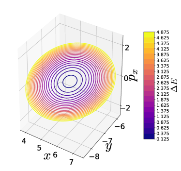
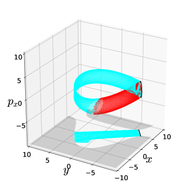
Figure 6: Unstable periodic orbits at interval of $\Delta E=0.25$ starting from $\Delta E=0.125$ around the bottom saddle equilibrium point. The stable and unstable manifolds associated with the unstable perioidic orbit (NHIM of dimension 1) around the same equilibrium point at $\Delta E=2.25$.

Numerical continuation to periodic orbit at arbitrary energy.— The procedure described above yields an accurate initial condition for a periodic orbit from a single initial guess. If our initial guess came from the linear approximation near the equilibrium point, from Eqn. (67), it has been observed numerically that we can only use this procedure for small amplitude, of order $10^{-4}$, periodic orbits around $\mathbf{x}_{\rm eq,bot}$. This small amplitude correspond to small excess energy, typically of the order $10^{-2}$, and if we want to compute the periodic orbit of arbitrarily large amplitude, we resort to numerical continuation for generating a family which reaches the appropriate total energy. This is done using two nearby periodic orbits of small amplitude to obtain initial guess for the next periodic orbit and performing differential correction to this guess. To this end, we proceed as follows. Suppose we find two small nearby periodic orbit initial conditions, $\bar{\mathbf{x}}_{0}^{(1)}$ and $\bar{\mathbf{x}}_{0}^{(2)}$, correct to within the tolerance $d_{\rm tol}$, using the differential correction procedure described above. We can generate a family of periodic orbits with successively increasing amplitudes around $\bar{\mathbf{x}}_{\rm eq,bot}$ in the following way. Let

$$\Delta=\bar{\mathbf{x}}_{0}^{(2)}-\bar{\mathbf{x}}_{0}^{(1)}=[\Delta x_{0},\Delta y_{0},0,0]^{T}$$ (40)

A linear extrapolation to an initial guess of slightly larger amplitude, $\bar{\mathbf{x}}_{0}^{(3)}$ is given by

$$\bar{\mathbf{x}}_{0,g}^{(3)}= ~{}\bar{\mathbf{x}}_{0}^{(2)}+\Delta$$ (41)

$$= \left[(\mathbf{x}_{0}^{(2)}+\Delta x_{0}),(y_{0}^{(2)}+\Delta y_{0}),0,0\right]^{T}$$ (42)

$$= \left[x_{0}^{(3)},y_{0}^{(3)},0,0\right]^{T}$$ (43)

Thus, keeping $x_{0}^{(3)}$ fixed, we can use differential correction on this initial condition to compute an accurate solution $\bar{\mathbf{x}}_{0}^{(3)}$ from the initial guess $\bar{\mathbf{x}}_{\rm 0,g}^{(3)}$ and repeat the process until we have a family of solutions. We can keep track of the energy of each periodic orbit and when we have two solutions, $\bar{\mathbf{x}}_{0}^{\rm(k)}$ and $\bar{\mathbf{x}}_{0}^{\rm(k+1)}$, whose energy brackets the appropriate energy, $E$, we can resort to combining bisection and differential correction to these two periodic orbits until we converge to the desired periodic orbit to within a specified tolerance. Thus, the result is a periodic orbit at desired total energy $E$ and of some period $T$ with an initial condition $X_{0}$. This is shown in Fig. 6 for a series of excess energy at intervals of 0.250.

Globalization of invariant manifolds — We find the local approximation to the unstable and stable manifolds of the periodic orbit from the eigenvectors of the monodromy matrix. Next, the local linear approximation of the unstable (or stable) manifold in the form of a state vector is integrated in the nonlinear equations of motion to produce the approximation of the unstable (or stable) manifolds. This procedure is known as globalization of the manifolds and we proceed as follows.

First, the state transition matrix $\Phi(t)$ along the periodic orbit with initial condition $X_{0}$ can be obtained numerically by integrating the variational equations along with the equations of motion from $t=0$ to $t=T$. This is known as the monodromy matrix $M=\Phi(T)$ and the eigenvalues can be computed numerically. For Hamiltonian systems (see Meyer, Hall, and Offin (2009) for details), tells us that the four eigenvalues of $M$ are of the form

$$\lambda_{1}>1,\qquad\lambda_{2}=\frac{1}{\lambda_{1}},\qquad\lambda_{3}=\lambda_{4}=1$$ (44)

The eigenvector associated with eigenvalue $\lambda_{1}$ is in the unstable direction, the eigenvector associated with eigenvalue $\lambda_{2}$ is in the stable direction. Let $e^{s}(X_{0})$ denote the normalized (to 1) stable eigenvector, and $e^{u}(X_{0})$ denote the normalized unstable eigenvector. We can compute the manifold by initializing along these eigenvectors as:

$$X^{s}(X_{0})=X_{0}+\epsilon e^{s}(X_{0})$$ (45)

for the stable manifold at $X_{0}$ along the periodic orbit as

$$X^{u}(X_{0})=X_{0}+\epsilon e^{u}(X_{0})$$ (46)

for the unstable manifold at $X_{0}$. Here the small displacement from $X_{0}$ is denoted by $\epsilon$ and its magnitude should be small enough to be within the validity of the linear estimate, yet not so small that the time of flight becomes too large due to asymptotic nature of the stable and unstable manifolds. Ref. Koon et al. (2011) suggests typical values of $\epsilon>0$ corresponding to nondimensional position displacements of magnitude around $10^{-6}$. By numerically integrating the unstable vector forwards in time, using both $\epsilon$ and $-\epsilon$, for the forward and backward branches respectively, we generate trajectories shadowing the two branches, $W^{u}_{+}$ and $W^{u}_{-}$, of the unstable manifold of the periodic orbit. Similarly, by integrating the stable vector backwards in time, using both $\epsilon$ and $-\epsilon$, for forward and backward branch respectively, we generate trajectories shadowing the stable manifold, $W^{s}_{+,-}$. For the manifold at $X(t)$, one can simply use the state transition matrix to transport the eigenvectors from $X_{0}$ to $X(t)$:

$$X^{s}(X(t))=\Phi(t,0)X^{s}(X_{0})$$ (47)

It is to be noted that since the state transition matrix does not preserve the norm, the resulting vector must be normalized. The globalized invariant manifolds associated with index-1 saddles are known as Conley-McGehee tubes (Marsden and Ross (2006)). These tubes form the skeleton of transition dynamics by acting as conduits for the states inside them to travel between potential wells.

The computation of codimension-1 separatrix associated with the unstable periodic orbit around a index-1 saddle begins with the linearized equations of motion. This is obtained after a coordinate transformation to the saddle equilibrium point and Taylor expansion of the equations of motion. Keeping the first order terms in this expansion, we obtain the eigenvalues and eigenvectors of the linearized system. The eigenvectors corresponding to the center direction provide the starting guess for computing the unstable periodic orbits for small excess energy, $\Delta E<<1$, above the saddle’s energy. This iterative procedure performs small correction to the starting guess based on the terminal condition of the periodic orbit until a desired tolerance is satisfied. This procedure is known as differential correction and generates unstable periodic orbits for small excess energy. Next, a numerical continuation is implemented to follow the small energy (amplitude) periodic orbits out to high excess energies. We apply this procedure to the Barbanis 2 DoF system in § II.1 to generate the unstable periodic orbit and its associated invariant manifolds as shown in Fig. 6.

A.2 The Linearized Hamiltonian System

To find the linearized equations around the saddle equilibria with coordinates $(x_{e},y_{e},0,0)$, we need the quadratic terms of the Hamiltonian (1) expanded about the equilibrium point. After making a coordinate change with $(x_{e},y_{e},0,0)$ as the origin, the quadratic terms of the Hamiltonian function for the linearized equations, which we shall call $H_{l}$, is given by

$$H_{l}=\frac{1}{2}p_{x}^{2}+\frac{1}{2}p_{y}^{2}+\frac{1}{2}\omega_{x}^{2}x^{2}+\frac{1}{2}\omega_{y}^{2}y^{2}+2\delta xyy_{e}+\delta y^{2}x_{e}$$ (48)

This gives the linear equations of motion near the equilibrium point as

$$\begin{pmatrix}\dot{x}\\ \dot{y}\\ \dot{p_{x}}\\ \dot{p_{y}}\end{pmatrix}=\begin{pmatrix}0&0&1&0\\ 0&0&0&1\\ -\omega_{x}^{2}&-2\delta y_{e}&0&0\\ -2\delta y_{e}&-(\omega_{y}^{2}+2\delta x_{e})&0&0\end{pmatrix}\begin{pmatrix}x\\ y\\ p_{x}\\ p_{y}\end{pmatrix}$$ (49)

A.2.1 Linear analysis near the equilibria

Studying the linearization of the dynamics near the equilibria is an essential ingredient for understanding the more full nonlinear dynamics. We analyze the linearized dynamics near the saddle equilibrium points which extends to the full nonlinear system due to the generalization of Liapounov’s theorem. Here we perform linearization of the vector field (18) to study the dynamics near the equilibrium points. This is given by the Jacobian, $Df(\mathbf{x})$, of the vector field

$$\mathbb{J}=Df(\mathbf{x})=\begin{pmatrix}0&0&1&0\\ 0&0&0&1\\ -\omega_{x}^{2}&-2\delta y_{e}&0&0\\ -2\delta y_{e}&-(\omega_{y}^{2}+2\delta x_{e})&0&0\end{pmatrix}$$ (50)

where $\mathbf{x}=(x,y,p_{x},p_{y})$ and $(x_{e},y_{e},0,0)$ is the equilibrium point.

Saddle-center equilibrium. — At the equilibria,

$$\left(-\frac{\omega_{y}^{2}}{2\delta},\pm\frac{1}{\sqrt{2}}\frac{\omega_{x}\omega_{y}}{\delta},0,0\right)$$ (51)

the Jacobian (50) becomes

$$\mathbb{J}= Df(\mathbf{x})\Bigr{|}_{\left(-\frac{\omega_{y}^{2}}{2\delta},\pm\frac{1}{\sqrt{2}}\frac{\omega_{x}\omega_{y}}{\delta},0,0\right)}$$ (52)

$$= \begin{pmatrix}0&0&1&0\\ 0&0&0&1\\ -\omega_{x}^{2}&\mp\sqrt{2}\omega_{x}\omega_{y}&0&0\\ \mp\sqrt{2}\omega_{x}\omega_{y}&0&0&0\end{pmatrix}$$

The characteristic polynomial of the Jacobian (52) can be expressed as

$${\rm det}(\mathbb{J}-\beta\mathbb{I})=p(\beta)=\beta^{4}+\omega_{x}^{2}\beta^{2}-2\omega_{x}^{2}\omega_{y}^{2}$$ (53)

Let $\alpha=\beta^{2}$, then the roots of the above polynomial are $\sqrt{\alpha_{1}},-\sqrt{\alpha_{1}},\sqrt{\alpha_{2}},-\sqrt{\alpha_{2}}$, where

$$\alpha_{1}= \frac{-\omega_{x}^{2}+\sqrt{\omega_{x}^{2}+8\omega_{x}^{2}\omega_{y}^{2}}}{2},$$ (54)

$$\alpha_{2}= \frac{-\omega_{x}^{2}-\sqrt{\omega_{x}^{2}+8\omega_{x}^{2}\omega_{y}^{2}}}{2}$$

It is clear that $\alpha_{1}>0$ and $\alpha_{2}<0$, so let us define, $\lambda=\sqrt{\alpha_{1}}$ and $\omega=\sqrt{-\alpha_{2}}$, so the eigenvalues are $\lambda,-\lambda,i\omega,-i\omega$. This implies the equilibrium point is of type saddle $\times$ center type, or index-1 saddle.

As shown above, the eigenvalues are of the form: $\lambda,-\lambda,i\omega,-i\omega$ where

$$\lambda^{2}=\alpha_{1}= \frac{-\omega_{x}^{2}+\sqrt{\omega_{x}^{2}+8\omega_{x}^{2}\omega_{y}^{2}}}{2}$$ (55)

$$\omega^{2}=-\alpha_{2}= \frac{\omega_{x}^{2}+\sqrt{\omega_{x}^{2}+8\omega_{x}^{2}\omega_{y}^{2}}}{2}$$

and the eigenvectors as obtained in § A.2.2 are

$$u_{\lambda}=\begin{bmatrix}1,&-\frac{\lambda^{2}+\omega_{x}^{2}}{\sqrt{2}\omega_{x}\omega_{y}},&\lambda,&-\frac{\lambda(\lambda^{2}+\omega_{x}^{2})}{\sqrt{2}\omega_{x}\omega_{y}}\end{bmatrix}$$ (56)

$$u_{-\lambda}=\begin{bmatrix}1,&-\frac{\lambda^{2}+\omega_{x}^{2}}{\sqrt{2}\omega_{x}\omega_{y}},&-\lambda,&\frac{\lambda(\lambda^{2}+\omega_{x}^{2})}{\sqrt{2}\omega_{x}\omega_{y}}\end{bmatrix}$$

and

$$w_{i\omega}= \begin{bmatrix}1,&\frac{\omega^{2}-\omega_{x}^{2}}{\sqrt{2}\omega_{x}\omega_{y}},&i\omega,&\frac{i\omega(\omega^{2}-\omega_{x}^{2})}{\sqrt{2}\omega_{x}\omega_{y}}\end{bmatrix}$$ (57)

$$w_{-i\omega}= \begin{bmatrix}1,&\frac{\omega^{2}-\omega_{x}^{2}}{\sqrt{2}\omega_{x}\omega_{y}},&-i\omega,&-\frac{i\omega(\omega^{2}-\omega_{x}^{2})}{\sqrt{2}\omega_{x}\omega_{y}}\end{bmatrix}$$

A.2.2 Eigenvectors of linearized system near index-1 saddle

Let us assume the eigenvector to be $v=[k_{1},k_{2},k_{3},k_{4}]^{T}$, and the eigenvalue problem becomes $\mathbb{J}v=\beta v$. This gives the expressions

$$k_{3}= \beta k_{1}$$ (58)

$$k_{4}= \beta k_{2}$$ (59)

$$-\omega_{x}^{2}k_{1}-\sqrt{2}\omega_{x}\omega_{y}k_{2}= \beta k_{3}$$ (60)

$$-\sqrt{2}\omega_{x}\omega_{y}k_{1}= \beta k_{4}$$ (61)

Let $k_{1}=1$, then using Eqns. (58)and (59) the eigenvector becomes $\bigl{[}1,k_{2},\beta,\beta k_{2}\bigr{]}$.

Then, using Eqns. (60)and (61) for eigenvalue $\beta=\pm\lambda$, we get

$$-\omega_{x}^{2}-\sqrt{2}\omega_{x}\omega_{y}k_{2}= \lambda^{2}$$ (62)

$$-\sqrt{2}\omega_{x}\omega_{y}= \lambda k_{2}$$

$$-\omega_{x}^{2}-\sqrt{2}\omega_{x}\omega_{y}k_{2}^{\prime}= \lambda^{2}$$

$$-\sqrt{2}\omega_{x}\omega_{y}= \lambda k_{2}^{\prime}$$

These imply, $k_{2}=k_{2}^{\prime}$ and

$$k_{2}=-\frac{\lambda^{2}+\omega_{x}^{2}}{\sqrt{2}\omega_{x}\omega_{y}}$$ (63)

A similar approach for the eigenvalues, $\beta=\pm\omega$, gives us

$$k_{2}=\frac{\omega^{2}-\omega_{x}^{2}}{\sqrt{2}\omega_{x}\omega_{y}}$$ (64)

Thus, the eigenvectors corresponding to $\pm\lambda$ are

$$u_{\lambda}=\begin{bmatrix}1,&-\frac{\lambda^{2}+\omega_{x}^{2}}{\sqrt{2}\omega_{x}\omega_{y}},&\lambda,&-\frac{\lambda(\lambda^{2}+\omega_{x}^{2})}{\sqrt{2}\omega_{x}\omega_{y}}\end{bmatrix}$$ (65)

$$u_{-\lambda}=\begin{bmatrix}1,&-\frac{\lambda^{2}+\omega_{x}^{2}}{\sqrt{2}\omega_{x}\omega_{y}},&-\lambda,&\frac{\lambda(\lambda^{2}+\omega_{x}^{2})}{\sqrt{2}\omega_{x}\omega_{y}}\end{bmatrix}$$

and for the eigenvalues, $\pm i\omega$, we obtain

$$w_{i\omega}= \begin{bmatrix}1,&\frac{\omega^{2}-\omega_{x}^{2}}{\sqrt{2}\omega_{x}\omega_{y}},&i\omega,&\frac{i\omega(\omega^{2}-\omega_{x}^{2})}{\sqrt{2}\omega_{x}\omega_{y}}\end{bmatrix}$$ (66)

$$w_{-i\omega}= \begin{bmatrix}1,&\frac{\omega^{2}-\omega_{x}^{2}}{\sqrt{2}\omega_{x}\omega_{y}},&-i\omega,&-\frac{i\omega(\omega^{2}-\omega_{x}^{2})}{\sqrt{2}\omega_{x}\omega_{y}}\end{bmatrix}$$

where $\lambda$ and $\omega$ are positive constants (54) that depend on the parameters of the potential energy surface. Thus, the general solution of the linear system near the saddle equilibrium point is given by

$$\mathbf{x}(t)= \left\{x(t),y(t),v_{x}(t),v_{y}(t)\right\}$$ (67)

$$= A_{1}e^{\lambda t}u_{\lambda}+A_{2}e^{-\lambda t}u_{-\lambda}+2{\rm Re}\left(\beta e^{i\omega t}w_{i\omega}\right)$$

with $A_{1},A_{2}$ being real and $\beta=\beta_{1}+i\beta_{2}$ being complex.

Appendix B Coupled harmonic 3 DoF system

For this system, Hamilton’s equations of motion are given by

$$\dot{x} =\frac{\partial V_{\rm BC}}{\partial p_{x}}=p_{x}$$ (68)

$$\dot{y} =\frac{\partial V_{\rm BC}}{\partial p_{y}}=p_{y}$$

$$\dot{z} =\frac{\partial V_{\rm BC}}{\partial p_{z}}=p_{z}$$

$$\dot{p}_{x} =-\frac{\partial V_{\rm BC}}{\partial x}=-(\omega_{x}^{2}x-2\epsilon xy-2\eta xz)$$

$$\dot{p}_{y} =-\frac{\partial V_{\rm BC}}{\partial y}=-(\omega_{y}^{2}y-\epsilon x^{2})$$

$$\dot{p}_{z} =-\frac{\partial V_{\rm BC}}{\partial z}=-(\omega_{z}^{2}z-\eta x^{2})$$

Linear analyis near equilibrium point — Here we study the dynamics near the equilibrium points using linearization of the vector field (68) given by the Jacobian, $Df(\mathbf{x})$, of the vector field evaluated at the equilibrium point, $\mathbf{x}_{\rm eq}=(x_{e},y_{e},z_{e},0,0,0)$.

$$\dot{\mathbf{x}}= \mathbb{J}\Bigr{|}_{\left(x_{e},y_{e},z_{e},0,0,0\right)}\mathbf{x}=Df(\mathbf{x})\Bigr{|}_{\left(x_{e},y_{e},z_{e},0,0,0\right)}\mathbf{x}$$ (69)

$$\dot{\mathbf{x}}= \begin{pmatrix}0&0&0&1&0&0\\ 0&0&0&0&1&0\\ 0&0&0&0&0&1\\ -(\omega_{x}^{2}-2\epsilon y_{e}-2\eta z_{e})&2\epsilon x_{e}&2\eta x_{e}&0&0&0\\ 2\epsilon x_{e}&-\omega_{y}^{2}&0&0&0&0\\ -2\eta x_{e}&0&-\omega_{z}^{2}&0&0&0\\ \end{pmatrix}\begin{bmatrix}x\\ y\\ z\\ p_{x}\\ p_{y}\\ p_{z}\end{bmatrix}$$

Symmetries of the equations of motion — We note the symmetries in the system (68), by substituting $(-x,-p_{x})$ for $(x,p_{x})$ which implies reflection about the $x=0$ plane and expressed as

$$s_{x}:(x,y,z,p_{x},p_{y},p_{z},t)\rightarrow(-x,y,z,-p_{x},p_{y},p_{z},t)$$ (70)

Thus, if $(x(t),y(t),z(t),p_{x}(t),p_{y}(t),p_{z}(t))$ is a solution to (68), then
$(-x(t),y(t),-p_{x}(t),p_{y}(t),p_{z}(t))$ is another solution. The conservative system also has time-reversal symmetry

$$s_{t}:(x,y,z,p_{x},p_{y},p_{z},t) \rightarrow(x,y,z,-p_{x},-p_{y},-p_{z},t)$$ (71)

So, if $(x(t),y(t),z(t),p_{x}(t),p_{y}(t),p_{z}(t))$ is a solution to (68), then
$(x(-t),y(-t),z(-t),-p_{x}(-t),-p_{y}(-t),-p_{z}(-t))$ is another solution. These symmetries will be used to decrease the number of computations, and to find special solutions. For example, any solution of (68) will evolve on the energy surface given by (4). For fixed energy, $E(x,y,z,p_{x},p_{y},p_{z})=e$, there will be zero velocity curves corresponding to $V_{BC}(x,y,z)=e$, the contours shown in Fig. 1. Any trajectory which touches the zero velocity curve at time $t_{0}$ must retrace its path in configuration space (i.e., $q=(x,y,z)$ space),

$$q(-t+t_{0})=q(t+t_{0})\qquad\mathring{q}(-t+t_{0})=-\mathring{q}(t+t_{0})$$ (72)