THREE DIMENSIONAL BLIND IMAGE DECONVOLUTION FOR FLUORESCENCE
MICROSCOPY USING GENERATIVE ADVERSARIAL NETWORKS
Abstract
Due to image blurring image deconvolution is often used for studying biological structures in fluorescence microscopy. Fluorescence microscopy image volumes inherently suffer from intensity inhomogeneity, blur, and are corrupted by various types of noise which exacerbate image quality at deeper tissue depth. Therefore, quantitative analysis of fluorescence microscopy in deeper tissue still remains a challenge. This paper presents a three dimensional blind image deconvolution method for fluorescence microscopy using -way spatially constrained cycle-consistent adversarial networks. The restored volumes of the proposed deconvolution method and other well-known deconvolution methods, denoising methods, and an inhomogeneity correction method are visually and numerically evaluated. Experimental results indicate that the proposed method can restore and improve the quality of blurred and noisy deep depth microscopy image visually and quantitatively.
Index Terms— image deconvolution, image restoration, fluorescence microscopy, generative adversarial networks, microscopy image quality
1 INTRODUCTION
Fluorescence microscopy is a modality that allows imaging of subcellular structures from live specimens [1, 2]. During this image acquisition process, large datasets of 3D microscopy image volumes are generated. The quantitative analysis of the fluorescence microscopy volume is hampered by light diffraction, distortion created by lens aberrations in different directions, complex variation of biological structures [3]. The image acquisition process can be typically modeled as the convolution of the observed objects with a 3D point spread function (PSF) followed by degradation from noise such as Poisson noise and Gaussian noise [4]. These limitations result in anisotropic, inhomogeneous background, blurry (out-of-focus), and noisy image volume with poor edge details which aggravate the image quality poorer in depth [5].
There has been various approaches to improve 3D fluorescence microscopy images quality. One popular approach is known as image deconvolution which “inverts” the convolution process to restore the original microscopy image volume [6]. Richard-Lucy (RL) deconvolution [7, 8] which maximizes the likelihood distribution based on a Poisson noise assumption for confocal microscopy was proposed. This RL deconvolution was further extended in [9] that incorporated the total variation as a regularization term in the cost function. Since the PSF is usually not known, blind deconvolution which estimates the PSF and the original image simultaneously is favorable [10]. Blind deconvolution using RL deconvolution was described in [11]. A pupil model for the PSF was presented in [12] and the PSF was estimated using machine learning approaches in [13]. Sparse coding to learn 2D features for coarse resolution along the depth axis to mitigate anisotropic issues was presented in [14].
Another approach to achieve better image quality stems from image denoising research. One example is Poisson noise removal using a combination of the Haar wavelet and the linear expansion of thresholds (PURE-LET) proposed in [15]. This PURE-LET approach was extended further to 3D widefield microscopy in [16]. Additionally, a denoising and deblurring method for Poisson noise corrupted data using variance stabilizing transforms (VST) was described in [17]. Meanwhile, a 3D inhomogeneity correction method that combines 3D active contours segmentation was presented in [18].
Convolutional neural network (CNN) has been popular to address various problems in medical image analysis and computer vision such as image denoising, image segmentation, and image registration [19]. There are few papers that focus on image deconvolution in fluorescence microscopy using CNNs. One example is an anisotropic fluorescence microscopy restoration method using a CNN [20]. Later, semi-blind spatially-variant deconvolution in optical microscopy with a local PSF using a CNN was described in [10]. More recently, generative adversarial networks has gradually gained interest in medical imaging especially for medical image analysis [21]. One of the useful architectures for medical image is a cycle-consistent adversarial networks (CycleGAN) [22] which learns image-to-image translation without having paired images (actual groundtruth images). This CycleGAN was utilized for CT denoising by an analogy of mapping low dose phase images to high dose phase images to improve image quality [23]. Additionally, this CycleGAN was further extended by [24] incorporating a spatial constrained term to minimize misalignment between synthetically generated binary volume and corresponding synthetic microscopy volume to achieve better segmentation results.
In this paper, we present a new approach to restore various biological structures in 3D microscopy images in deeper tissue without knowing the 3D PSF using a spatially constrained CycleGAN (SpCycleGAN) [24]. We train and inference the SpCycleGAN in three directions along with , , and sections (-Way SpCycleGAN) to incorporate 3D information inspired by [25, 26]. These restored -way microscopy images are then averaged and evaluated with three different image quality metrics. Our datasets consist of Hoechst labeled nuclei and a phalloidin labeled filamentous actin collected from a rat kidney using two-photon microscopy. The goal is to restore blurred and noisy 3D microscopy images to the level of well-defined images so that the deeper depth tissues can be used for biological study.
2 PROPOSED METHOD
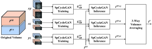
Figure 1 shows a block diagram of the proposed 3D images deconvolution method. We denote as a 3D image volume of size . Note that is a section with focal plane along the -direction in a volume, where . Similarly, is a section with focal plane along -direction, where , and is a section with focal plane along -direction, where . In addition, let be a subvolume of , whose -coordinate is , -coordinate is , and -coordinate is . For example, is a subvolume of where the subvolume is cropped between slice and slice in -direction, between slice and slice in -direction, and between slice and slice in -direction.
As shown in Figure 1, we divide an original florescence microscopy volume denoted as into two subvolumes such as an out-of-focus and noisy subvolume and a well-defined subvolume denoted as and , respectively. In particular, we choose from deep sections and from shallow sections since shallow sections of fluorescence microscopy volumes typically have a better image quality than deep sections. These two volumes are sliced in the -, -, and -direction to form the , , and sections of the images. Then, the sections from and are used for the training of the SpCycleGAN [24] to obtain the trained generative network denoted as . Similarly doing this with the sections and the sections, trained generative networks and are obtained. These generative networks are used for inference with a test volume denoted as in the , , and sections. Next, these synthetically generated results by the SpCycleGAN inference are stacked with -, -, and -direction to form 3D volumes denoted as , , and , respectively. Finally, we obtain the final volume by voxelwise weighted averaging of these volumes.
2.1 Spatially Constrained CycleGAN (SpCycleGAN)
This SpCycleGAN was introduced in our previous work [24] which extended the CycleGAN [22] by adding one more term to the loss function and introducing an additional generative network. The SpCycleGAN was used for generating synthetic microscopy volumes from a synthetic binary volume. One problem with the CycleGAN is that the generated images sometimes are misaligned with the input images. We added a spatial constrained term () to the loss function and minimize the loss function together with the two original GAN losses () and the cycle consistent loss () as:
| (1) |
where
Note that and are the controllable coefficients for and . Also, and represent and norms, respectively.
The generative model transfers to and the generative model transfers to .
Similarly, the discriminative model and distinguish between and and between and .
In particular, is a transfer function using model and is another transfer function using model .
For example, is a synthetically restored volume generated by model using a blurred and noisy volume. Also, is a synthetically generating blurred and noisy volume by model using a well-defined volume. Additionally, another generative model takes as an input to generate a synthetically blurred and noisy volume using synthetically restored volume. This generative model minimizes loss between and .


2.2 3-Way SpCycleGAN and Volumes Averaging
One drawback of the SpCycleGAN is that it works only in 2D. Since our fluorescence microscopy data is a 3D volume, we form the 3D volume by stacking 2D images obtained from different focal planes during data acquisition [27]. Therefore, we employ -Way SpCycleGAN training which uses the SpCycleGAN in the , , and sections independently and obtain the generative models per each sections. We use three generative models (, , and ) for the inference using which transfer noisy and out-of-focus images to well-defined and focused images in the , , and sections. More specifically, the test volume is sliced into three sets of sectional images and each image is used as an input of inference to generate synthetic well-defined and focused image. Then, these synthetically generated images are stacked in the -, -, and -direction to form , , and , respectively. In general, the number of the , , and sections are different from each other, we use zero padding to make the dimension of three volumes identical. Lastly, the final volume () is obtained as
| (2) |
where , , and are weight coefficients of , , and , respectively.
3 EXPERIMENTAL RESULTS
The performance of our proposed deconvolution method was tested on two different datasets:111Dataset-I and II were provided by Malgorzata Kamocka of the Indiana Center for Biological Microscopy. Dataset-I and II. Dataset-I and II are originally obtained at the same time with different fluorophores to delineate different biological structures. Dataset-I and II are both comprised of grayscale images, each of size pixels. We selected a blurred and noisy subvolume () from last images of given fluorescence microscopy volume as with a size of for Dataset-I and II. Also, a good quality subvolume () was selected based on a biologist’s opinion as with size of for Dataset-I and II. The test volume () for each dataset was selected at deeper tissue depth than as with size of .
Our -Way SpCycleGAN is implemented in PyTorch using the Adam optimizer [28] with constant learning rate for the first epochs and gradually decreased to for the next epochs. Also, we use the ResNet blocks [29] for all generative models (, , and ) with feature maps at the first layer. For the corresponding discriminative models ( and ), same discriminative models are used in the CycleGAN [22]. We randomly select patches size of from for the sections and from for the and sections for the SpCycleGAN training, respectively. We choose larger resolution for the sections since sections is a finer resolution than those and sections. Also, we set the coefficients for all -Way SpCycleGAN training for both Dataset-I and II. Lastly, the weights for -way volume averaging is set as so that each sectional results equally contribute the final volume.
| of the Dataset-I | of the Dataset-II | |||||
| Method | 3-Way | 3-Way | 3-Way | 3-Way | 3-Way | 3-Way |
| BRISQUE [30] | OG-IQA [31] | Microscopy IFQ [32] | BRISQUE [30] | OG-IQA [31] | Microscopy IFQ [32] | |
| RL [7, 8] | ||||||
| EpiDEMIC [14] | ||||||
| PureDenoise [15] | ||||||
| iterVSTpoissonDeb [17] | ||||||
| 3DacIC [18] | ||||||
| 3-Way SpCycleGAN | ||||||
| (Proposed) | ||||||
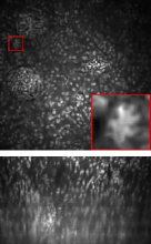
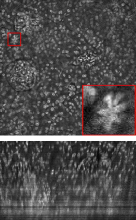
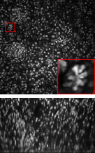
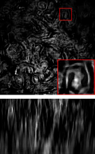
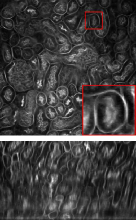
Our proposed deconvolution results were visually compared with five different techniques including RL [7, 8], EpiDEMIC [14], PureDenoise [15], iterVSTPoissonDeb [17], and 3DacIC [18] shown in Figure 2. Note that we used default settings for the methods RL and PureDenoise in ImageJ plugins, EpiDEMIC in Icy plugin, and iterVSTpoissonDeb.
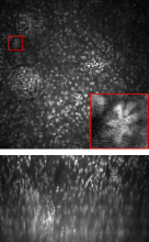
As shown in Figure 2, first column displays a sample section () and section () of original test volumes in Dataset-I and II, respectively. The original test volumes suffer from significant intensity inhomogeneity, blur, and noise. Also, this degradation gets worse at deeper depth as shown in the section. As observed, our proposed method showed the best performance among presented methods in terms of inhomogeneity correction, clarity of the shape of nuclei and tubules/glomeruli structure, and noise level. More specifically, two deconvolution methods (RL and EpiDEMIC) successfully reduced blur but the original shapes of the biological structures were lost. Also, EpiDEMIC’s section deconvolution results were all connected each other since EpiDEMIC learned 2D features as a prior to enhance 3D. Similarly, two denoising methods (PureDenoise and iterVSTpoissonDeb) successfully suppressed Poisson noise but these denoising results were still suffered from intensity inhomogeneity and blur. In fact, the denoising results added more blur than original test volume. Meanwhile, 3DacIC method successfully corrected inhomogeneity but this method amplified background noise level and aggravated image quality. Moreover, 3DacIC exacerbated line shape noise shown in the sections.
In addition to the visual comparison, three image quality metrics were utilized for evaluating volume quality of restored volumes of proposed and other presented methods. Since our microscopy volumes do not have reference volumes to compare, we need to use no reference image quality assessment (NR-IQA) [30] instead of traditional PSNR, SSIM, and FSIM. One problem is that there is no gold standard image quality metric for 3D fluorescence microscopy. We employed the blind/referenceless image spatial quality evaluator (BRISQUE) [30], the oriented-gradient image quality assessment (OG-IQA) [31], and the microscopy image focus quality assessment (Microscopy IFQ) [32] for evaluating quality of restored microscopy volumes. In particular, BRISQUE model is a regression model learned from local statistics of natural scenes in the spatial domain to measure image quality where the quality value range is from to . OG-IQA model is a gradient feature based model that maps from image features to image quality via an adaboosting back propagation neural network where the quality value is from to . Lastly, Microscopy IFQ measures discrete defocus level from to using local patches using a CNN. Instead of using discrete defocus level, we got a probability () for each corresponding defocus level () before the softmax layer and used these probabilities and corresponding defocus levels to obtain expected value which defined as
| (3) |
Since this Microscopy IFQ value was obtained for each individual local patches, we resized our images to be nearest integer multiple of local patch size and took an average through entire image. Note that the smaller values of all three image quality assessments indicate the better image quality. In addition, since these three image quality assessments can only measure the quality of 2D images, we again utilized -way idea to obtain the image quality of the , , and sections and took an average of them. The end result was a single representative value for volume quality per each volume.
We used these three image quality metrics to test seven different volumes including the original test volume. This is provided in Table 1. Note that we selected the most blurred and noisy image volumes from test volume as for the evaluation purpose. As mentioned above the smaller values are considered to be indicators of the better image volume quality. As observed in Table 1, our proposed method outperformed the other methods and original volume except from -Way BRISQUE in Dataset-II. This is because BRISQUE measures the quality from natural image statistics and this model is a favor of blurred volume. Therefore, RL and EpiDEMIC had higher values in BRISQUE image quality metric. Similarly, OG-IQA is a gradient based measurement so edge preserved restoration volume can get smaller image quality values. Also, Microscopy IFQ is a defocus level measurement. Hence, PureDenoise and iterVSTpoissonDeb had sometimes higher OG-IQA and Microscopy IFQ. 3DacIC produced reasonably lower values for the sections but the quality of the and sections were poor so that the entire volume quality was inferior than proposed method’s volume quality.
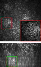
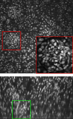
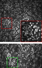
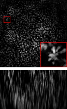
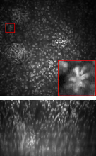
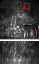
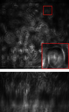
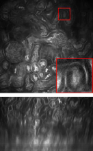
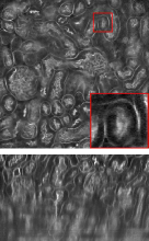
Lastly, Figure 3 portrays the visual comparison between proposed -Way SpCycleGAN and SpCycleGAN using the sections only (, ). Without having -direction information, SpCycleGAN using the sections cannot correctly restore the glomerulus displayed in the red box. Also, the -direction images are frequently discontinued as shown in the section in the green box. Compared to that, proposed -Way SpCycleGAN can successfully restore glomerulus and connect smoothly in -direction.
4 CONCLUSION AND FUTURE WORK
This paper has presented a blind image deconvolution method for fluorescence microscopy volumes using the -Way SpCycleGAN. Using the -Way SpCycleGAN, we can successfully restore the blurred and noisy volume to good quality volume so that deeper volume can be used for the biological research. Future work will include developing a 3D segmentation technique using our proposed deconvolution method as a preprocessing step.
References
- [1] D. W. Piston, “Imaging living cells and tissues by two-photon excitation microscopy,” Trends in Cell Biology, vol. 9, no. 2, pp. 66–69, February 1999.
- [2] C. Vonesch, F. Aguet, J. Vonesch, and M. Unser, “The colored revolution of bioimaging,” IEEE Signal Processing Magazine, vol. 23, no. 3, pp. 20–31, May 2006.
- [3] D. B. Murphy and M. W. Davidson, Fundamentals of Light Microscopy and Electronic Imaging, Wiley-Blackwell, Hoboken, NJ, 2nd edition, 2012.
- [4] S. Yang and B. U. Lee, “Poisson-Gaussian noise reduction using the hidden Markov model in contourlet domain for fluorescence microscopy images,” PLOS ONE, vol. 10, no. 9, pp. 1–19, September 2015.
- [5] S. Lee, C. Fu, P. Salama, K. W. Dunn, and E. J. Delp, “Tubule segmentation of fluorescence microscopy images based on convolutional neural networks with inhomogeneity correction,” Proceedings of the IS&T International Symposium on Electronic Imaging, vol. 2018, no. 15, pp. 199–1–199–8, January 2018, Burlingame, CA.
- [6] P. Sarder and A. Nehorai, “Deconvolution methods for 3-D fluorescence microscopy images,” IEEE Signal Processing Magazine, vol. 23, no. 3, pp. 32–45, May 2006.
- [7] W. H. Richardson, “Bayesian-based iterative method of image restoration,” Journal of the Optical Society of America, vol. 62, no. 1, pp. 55–59, January 1972.
- [8] L. B. Lucy, “An iterative technique for the rectification of observed distributions,” The Astronomical Journal, vol. 79, no. 6, pp. 745–754, June 1974.
- [9] N. Dey, L. Blanc-Feraud, C. Zimmer, P. Roux, Z. Kam, J.-C. Olivo-Marin, and J. Zerubia, “Richardson-Lucy algorithm with total variation regularization for 3D confocal microscope deconvolution,” Microscopy Research and Technique, vol. 69, no. 4, pp. 260–266, April 2006.
- [10] A. Shajkofci and M. Liebling, “Semi-blind spatially-variant deconvolution in optical microscopy with local point spread function estimation by use of convolutional neural networks,” Proceedings of the IEEE International Conference on Image Processing, pp. 3818–3822, October 2018, Athens, Greece.
- [11] D. A. Fish, A. M. Brinicombe, E. R. Pike, and J. G. Walker, “Blind deconvolution by means of the Richardson-Lucy algorithm,” Journal of the Optical Society of America A, vol. 12, no. 1, pp. 58–65, January 1995.
- [12] F. Soulez, L. Denis, Y. Tourneur, and E. Thiebaut, “Blind deconvolution of 3D data in wide field fluorescence microscopy,” Proceedings of the IEEE International Symposium on Biomedical Imaging, pp. 1735–1738, May 2012, Barcelona, Spain.
- [13] T. Kenig, Z. Kam, and A. Feuer, “Blind image deconvolution using machine learning for three-dimensional microscopy,” IEEE Transactions on Pattern Analysis and Machine Intelligence, vol. 32, no. 12, pp. 2191–2204, December 2010.
- [14] F. Soulez, “A learn 2D, apply 3D method for 3D deconvolution microscopy,” Proceedings of the IEEE International Symposium on Biomedical Imaging, pp. 1075–1078, April 2014, Beijing, China.
- [15] F. Luisier, C. Vonesch, T. Blu, and M. Unser, “Fast interscale wavelet denoising of Poisson-corrupted images,” Signal Processing, vol. 90, no. 2, pp. 415–427, February 2010.
- [16] J. Li, F. Luisier, and T. Blu, “PURE-LET deconvolution of 3D fluorescence microscopy images,” Proceedings of the IEEE International Symposium on Biomedical Imaging, pp. 723–727, April 2017, Melbourne, Australia.
- [17] L. Azzari and A. Foi, “Variance stabilization in Poisson image deblurring,” Proceedings of the IEEE International Symposium on Biomedical Imaging, pp. 728–731, April 2017, Melbourne, Australia.
- [18] S. Lee, P. Salama, K. W. Dunn, and E. J. Delp, “Segmentation of fluorescence microscopy images using three dimensional active contours with inhomogeneity correction,” Proceedings of the IEEE International Symposium on Biomedical Imaging, pp. 709–713, April 2017, Melbourne, Australia.
- [19] G. Litjens, T. Kooi, B. E. Bejnordi, A. A. A. Setio, F. Ciompi, M. Ghafoorian, J. A. van der Laak, B. van Ginneken, and C. I. Sanchez, “A survey on deep learning in medical image analysis,” Medical Image Analysis, vol. 42, no. 1, pp. 60–88, December 2017.
- [20] M. Weigert, L. Royer, F. Jug, and G. Myers, “Isotropic reconstruction of 3D fluorescence microscopy images using convolutional neural networks,” Proceedings of the International Conference on Medical Image Computing and Computer Assisted Intervention, pp. 126–134, September 2017, Quebec, Canada.
- [21] X. Yi, E. Walia, and P. Babyn, “Generative adversarial network in medical imaging: A review,” arXiv preprint arXiv:1809.07294, pp. 1–20, September 2018.
- [22] J. Y. Zhu, T. Park, P. Isola, and A. A. Efros, “Unpaired image-to-image translation using cycle-consistent adversarial networks,” Proceedings of the IEEE International Conference on Computer Vision, pp. 2242–2251, October 2017, Venice, Italy.
- [23] E. Kang, H. J. Koo, D. H. Yang, J. B. Seo, and J. C. Ye, “Cycle consistent adversarial denoising network for multiphase coronary CT angiography,” arXiv preprint arXiv:1806.09748, pp. 1–9, June 2018.
- [24] C. Fu, S. Lee, D. J. Ho, S. Han, P. Salama, K. W. Dunn, and E. J. Delp, “Three dimensional fluorescence microscopy image synthesis and segmentation,” Proceedings of the IEEE Conferences on Computer Vision and Pattern Recognition Workshop, pp. 2302–2310, June 2018, Salt Lake City, UT.
- [25] H. R. Roth, L. Lu, A. Seff, K. M. Cherry, J. Hoffman, S. Wang, J. Liu, E. Turkbey, and R. M. Summers, “A new 2.5D representation for lymph node detection using random sets of deep convolutional neural network observations,” Proceedings of the International Conference on Medical Image Computing and Computer Assisted Intervention, pp. 520–527, September 2014, Boston, MA.
- [26] S. Lee and D. Kim, “Background subtraction using the factored 3-way restricted Boltzmann machines,” arXiv preprint arXiv:1802.01522, pp. 1–10, February 2018.
- [27] D. Sage, L. Donati, F. Soulez, D. Fortun, G. Schmit, A. Seitz, R. Guiet, C. Vonesch, and M. Unser, “DeconvolutionLab2: An open-source software for deconvolution microscopy,” Methods, vol. 115, no. 1, pp. 28–41, February 2017.
- [28] D. P. Kingma and J. L. Ba, “Adam: A method for stochastic optimization,” arXiv preprint arXiv:1412.6980, pp. 1–15, January 2017.
- [29] K. He, X. Zhang, S. Ren, and J. Sun, “Deep residual learning for image recognition,” Proceedings of the IEEE Conference on Computer Vision and Pattern Recognition, pp. 770–778, June 2016, Las Vegas, NV.
- [30] A. Mittal, A. K. Moorthy, and A. C. Bovik, “No-reference image quality assessment in the spatial domain,” IEEE Transactions on Image Processing, vol. 21, no. 12, pp. 4695–4708, December 2012.
- [31] L. Liu, Y. Hua, Q. Zhao, H. Huang, and A. C. Bovik, “Blind image quality assessment by relative gradient statistics and adaboosting neural network,” Signal Processing: Image Communication, vol. 40, no. 1, pp. 1–15, January 2016.
- [32] S. J. Yang, M. Berndl, D. Michael Ando, M. Barch, A. Narayanaswamy, E. Christiansen, S. Hoyer, C. Roat, J. Hung, C. T. Rueden, A. Shankar, S. Finkbeiner, and P. Nelson, “Assessing microscope image focus quality with deep learning,” BMC Bioinformatics, vol. 19, no. 1, pp. 77–1–9, March 2018.