ICT Capital–Skill Complementarity and Wage Inequality:
Evidence from OECD Countries

Abstract

Although wage inequality has evolved in advanced countries over recent decades, it remains unknown the extent to which changes in wage inequality and their differences across countries are attributable to specific capital and labor quantities. We examine this issue by estimating a sector-level production function extended to allow for capital–skill complementarity and factor-biased technological change using cross-country and cross-industry panel data. Our results indicate that most of the changes in the skill premium are attributable to the relative quantities of ICT equipment, skilled labor, and unskilled labor in the goods and service sectors of the majority of advanced countries.

Keywords: Skill premium; capital–skill complementarity; technological change; information and communication technology (ICT); production function.
JEL classification: C33, E24, J24, J31, O50.

1 Introduction

One of the greatest changes in production activities over recent decades is the introduction and expansion of information and communication technology (ICT). The prevalence of new technology could result in a change in the relative demand for different types of labor, and thus, a change in their relative wages. According to the concept of capital–skill complementarity (Griliches, 1969), if ICT equipment is more complementary to skilled labor than unskilled labor, the increased use of ICT would raise the relative demand for skilled to unskilled labor, and thus, the relative wages of skilled to unskilled labor. Nevertheless, it is unknown the extent to which the increased use of ICT can account for changes in the relative wages of skilled to unskilled labor in many advanced countries.

We examine this issue by estimating a sector-level production function extended to allow for complementarity between ICT and skills. Our approach builds upon the aggregate production function developed by Fallon and Layard (1975) and Krusell, Ohanian, Rios-Rull, and Violante (2000). We focus on the relative wages of skilled to unskilled labor, which is referred to as the skill premium or sometimes as the college premium. The skill premium is a key metric used to evaluate the level of wage inequality and its differences across countries. Changes in the skill premium can be interpreted as the outcome of the race between supply shifts due to advances in education and demand shifts due to developments in technology (Tinbergen, 1974; Goldin and Katz, 2010), and thus, can be decomposed into a part due to shifts in the relative supply of skills and a part due to shifts in the relative demand for skills. We refer to the supply shifts as the relative labor quantity effect. The advantage of our approach is that it enables us to decompose the demand shifts into a part attributable to observed factors such as specific capital and labor quantities and a part attributable to unobserved factors such as factor-augmenting technology. We refer to the former as the capital–skill complementarity effect and the latter as the relative factor-augmenting technology effect. Consequently, we can evaluate the extent to which changes in the skill premium are attributable to the expansion of ICT equipment. The impact of policies that increase skilled labor depends on the mechanisms through which the skill premium has changed over recent decades. This study aims to expand our understanding of the sources and mechanisms of changes in the skill premium by measuring the quantitative contribution of the three effects to changes in the skill premium in the goods and service sectors of advanced countries.

For this purpose, we make use of cross-country and cross-industry panel data from 14 OECD countries for the years 1970 to 2005. This brings two major advantages to the analysis. First, we can exploit large variation in relative factor quantities across countries over time, which helps identify the elasticities of substitution between different types of capital and labor in production. In doing so, we exploit demand shocks in the service (goods) sector as a source of exogenous variation in factor supply in the goods (service) sector. Second, we can examine the sources and mechanisms of the differences in changes in the skill premium across countries. It is unclear from the literature the extent to which international differences in changes in the skill premium can be attributed to specific capital and labor quantities. Using the estimated production function, we decompose the sources of differences in changes in the skill premium across countries, as well as those of changes in the skill premium for each country and sector.

The main findings of this study can be summarized as follows. First, the estimated elasticity of substitution between ICT equipment and skilled labor is much smaller than that between ICT equipment and unskilled labor. This result supports the capital–skill complementarity hypothesis that ICT equipment is more complementary to skilled labor than unskilled labor. Second, the capital–skill complementarity effect associated with a rise in ICT equipment is large enough to account for a rise in the skill premium in the goods and service sectors of most OECD countries. The capital–skill complementarity effect is greater for the goods sector than the service sector in most OECD countries. Third, when ICT equipment is distinguished from non-ICT capital, changes in the skill premium are attributable mainly to observed capital and labor quantities in the goods and service sectors of the majority of OECD countries. Fourth, as its consequences, a large part of the differences in changes in the skill premium among those countries can be explained by the relative quantities of ICT equipment, skilled labor, and unskilled labor. Fifth, a rise in the relative demand for skilled to unskilled labor is attributable to a fall in the rental price of ICT equipment in the goods and service sectors of most OECD countries. Finally, a rise in skilled labor has a greater effect on reducing the skill premium in the presence than in the absence of capital–skill complementarity. This result points to the possibility that the contribution of higher education expansion to reducing the skill premium would be understated if capital–skill complementarity is not taken into account.

The remainder of this paper is organized as follows. The next section briefly reviews the related literature. Section 3 presents the sector-level production function used to account for changes in the skill premium. Section 4 describes the data and variables used in the analysis. Section 5 outlines the econometric specifications and techniques. Section 6 discusses the estimation results and their implications. The final section provides a summary and conclusions.

2 Related Literature

A cornerstone for the analysis of the skill premium has been the aggregate production function. Bound and Johnson (1992) and Katz and Murphy (1992) estimate an aggregate production function with two types of labor (skilled and unskilled labor) to understand the sources and mechanisms of changes in the skill premium in the United States from the 1960s or 1970s to the 1980s. These studies demonstrate that changes in the skill premium are partially attributable to the relative quantity of skilled labor but mostly to skill-biased technological change. For a given elasticity of substitution between skilled and unskilled labor, Acemoglu (2003) and Caselli and Coleman (2006) measure relative labor-augmenting technology in many countries using an aggregate production function with two types of labor. These studies consider cross-country differences in changes in the skill premium as a consequence of the differences in the direction of technological change.

Krusell et al. (2000) develop and estimate a four-factor production function in which not only skilled labor is distinguished from unskilled labor, but also capital equipment is distinguished from capital structure. They demonstrate that capital equipment is more complementary to skilled labor than unskilled labor, and attribute the rise in the skill premium in the United States from the years 1963 to 1992 mainly to a rise in capital equipment. Lindquist (2005) finds similar results to Krusell et al. (2000) in Sweden. Caselli and Coleman (2002) measure labor-augmenting technology in the United States during the same period using the same production function as in Krusell et al. (2000). They find that technological change was biased towards skilled labor.

A cornerstone for the analysis of the impact of ICT on demand for skills has been the factor-share equations derived from the translog cost or production function. Autor, Katz, and Krueger (1998) find that the wage-bill share of skilled labor increased with a rise in the proportion of workers using computers in the United States between the years 1984 and 1993. Michaels, Natraj, and Van Reenen (2014) find that the wage-bill share of high-skilled labor increased with a rise in ICT equipment in 11 OECD countries between the years 1980 and 2004, while the wage-bill share of medium-skilled labor decreased. Ruiz-Arranz (2003) confirms the presence of capital–skill complementarity when information technology equipment is distinguished from other types of capital. However, her results suggest that more than half of the rise in the skill premium in the United States between the years 1965 and 1999 is attributable to unobserved factors. Perez-Laborda and Perez-Sebastian (2020) find similar results to Ruiz-Arranz (2003) in many sectors of the United States between the years 1970 and 2005 when ICT equipment is distinguished from non-ICT capital.

A growing body of research focuses on the allocation of skills to tasks to examine the impact of new technology on the labor market. Autor, Levy, and Murnane (2003) find that the increased share of non-routine tasks and the decreased share of routine tasks are associated with the widespread use of computers. Their results suggest that more than half of the increased demand for skilled relative to unskilled labor in the United States between the years 1970 and 1998 is attributable to changes in the task composition. Acemoglu and Autor (2011) emphasize the importance of distinguishing between skills and tasks to shed light on some phenomena such as the polarization of employment and wages, while recognizing the value of the canonical model of the race between education and technology for the analysis of wage inequality. Eden and Gaggl (2018) estimate an aggregate production function in which capital is divided into ICT and non-ICT capital and labor is divided into routine and non-routine tasks. They demonstrate that about half of the decline in the labor income share in the United States between the years 1950 and 2013 is attributable to a rise in the income share of ICT equipment.

Acemoglu (2002) notes that skill-biased technological change is a threat to the identification of capital–skill complementarity when using time-series data from a single country. Duffy, Papageorgiou, and Perez-Sebastian (2004) estimate a three-factor production function with one type of capital and two types of labor using cross-country panel data from the Penn World Tables 5.6, and partially confirm the capital–skill complementarity hypothesis. However, the data used in their study do not contain information on wages. Karabarbounis and Neiman (2014) estimate the elasticity of substitution between capital and labor using cross-country panel data from multiple sources on the labor share of income and the relative price of investment to consumption goods, and demonstrate that about half of the global decline in the labor share of income between the years 1975 and 2012 is attributable to a fall in the relative price of investment.

Compared with previous studies, this study aims to examine the extent to which the expansion of ICT equipment can account for changes in the skill premium for each country and sector and the differences in such changes across countries. For this purpose, we estimate a sector-level production function with two types of capital (ICT and non-ICT capital) and two types of labor (skilled and unskilled labor) using data from a panel of OECD countries.

3 The Model

We start our analysis by considering a four-factor production function with capital–skill complementarity. Perhaps surprisingly, the production function presented here has not been estimated using cross-country panel data.

3.1 Production function

The economy consists of two sectors: goods and services. We assume that the output ($y$) is produced by a constant-returns-to-scale technology using ICT capital ($k_{i}$), non-ICT capital ($k_{o}$), skilled labor ($\ell_{h}$), and unskilled labor ($\ell_{u}$) for each sector. Following Fallon and Layard (1975) and Krusell et al. (2000), the four-factor production function is specified as

$$y=Ak_{o}^{\alpha}\left\{\lambda\left[\mu k_{i}^{\rho}+\left(1-\mu\right)\ell_{h}^{\rho}\right]^{\frac{\sigma}{\rho}}+\left(1-\lambda\right)\ell_{u}^{\sigma}\right\}^{\frac{1-\alpha}{\sigma}}\qquad\text{for }\sigma,\rho<1,$$ (1)

where $A$ is factor-neutral technology. The parameter $\sigma$ governs the degree of substitution between the $k_{i}$-$\ell_{h}$ composite and $\ell_{u}$, while the parameter $\rho$ governs the degree of substitution between $k_{i}$ and $\ell_{h}$. Production technology exhibits capital–skill complementarity if ICT capital is more complementary to, or less substitutable with, skilled labor than unskilled labor ($\sigma>\rho$). The specification of the production function (1) is consistent with the data in the sense that the parameter estimates satisfy $\sigma<1$ and $\rho<1$. The advantage of this approach over the translog approach is that it enables us to incorporate many factors with a small number of parameters and directly relate the skill premium to relative factor quantities.

The four-factor production function can also be represented as

$$f\left(k_{i},k_{o},\ell_{h},\ell_{u}\right)=k_{o}^{\alpha}\left\{\left[\left(A_{i}k_{i}\right)^{\rho}+\left(A_{h}\ell_{h}\right)^{\rho}\right]^{\frac{\sigma}{\rho}}+\left(A_{u}\ell_{u}\right)^{\sigma}\right\}^{\frac{1-\alpha}{\sigma}},$$ (2)

where factor-augmenting technology has the following form: $A_{i}=A^{\frac{1}{1-\alpha}}\lambda^{\frac{1}{\sigma}}\mu^{\frac{1}{\rho}}$, $A_{h}=A^{\frac{1}{1-\alpha}}\lambda^{\frac{1}{\sigma}}(1-\mu)^{\frac{1}{\rho}}$, and $A_{u}=A^{\frac{1}{1-\alpha}}(1-\lambda)^{\frac{1}{\sigma}}$. Let $w_{h}$ and $w_{u}$ denote the wages of skilled and unskilled labor, respectively, and $r_{i}$ and $r_{o}$ denote the rental prices of ICT and non-ICT capital, respectively. Profit maximization entails equating the value of marginal product with the marginal cost.

$$w_{h} = \omega_{h}\frac{\partial f}{\partial\ell_{h}},$$ (3)

$$w_{u} = \omega_{u}\frac{\partial f}{\partial\ell_{u}},$$ (4)

$$r_{i} = \omega_{i}\frac{\partial f}{\partial k_{i}},$$ (5)

$$r_{o} = \omega_{o}\frac{\partial f}{\partial k_{o}},$$ (6)

where $\omega$ is the wedge that represents the deviation from the profit-maximizing conditions in competitive markets. We allow the size of the wedge to differ across factor markets. Appendix A.1 provides a detailed derivation of the first-order conditions.

The first-order conditions (3) and (4) imply that the relative wages of skilled to unskilled labor are proportional to the marginal rate of technical substitution of unskilled for skilled labor. After simple algebra, the relative wages of skilled to unskilled labor are given by

$$\ln\left(\frac{w_{h}}{w_{u}}\right)=\sigma\ln\left(\frac{A_{h}}{A_{u}}\right)+\frac{\sigma-\rho}{\rho}\ln\left[\left(\frac{A_{i}k_{i}}{A_{h}\ell_{h}}\right)^{\rho}+1\right]-\left(1-\sigma\right)\ln\left(\frac{\ell_{h}}{\ell_{u}}\right)+\ln\left(\frac{\omega_{h}}{\omega_{u}}\right).$$ (7)

Within a reasonable range of parameter values ($0<\sigma<1$ and $\sigma>\rho$), the skill premium ($w_{h}/w_{u}$) increases with the ratio of skilled to unskilled labor-augmenting technology ($A_{h}/A_{u}$), the ratio of ICT capital- to skilled labor-augmenting technology ($A_{i}/A_{h}$), and the ratio of ICT capital to skilled labor ($k_{i}/\ell_{h}$) but decreases with the ratio of skilled to unskilled labor ($\ell_{h}/\ell_{u}$), holding the relative wedge ($\omega_{h}/\omega_{u}$) constant. We refer to the sum of the first and second effects associated with unobserved technology ($A_{h}/A_{u}$ and $A_{i}/A_{h}$) as the relative factor-augmenting technology effect. We refer to the third and fourth effects associated with observed factors ($k_{i}/\ell_{h}$ and $\ell_{h}/\ell_{u}$) as the capital–skill complementarity effect and the relative labor quantity effect, respectively. The capital–skill complementarity effect is proportional in magnitude to the difference in substitution parameters ($\sigma-\rho$), as well as $k_{i}/\ell_{h}$. The relative labor quantity effect is inversely proportional in magnitude to the substitution parameter $\sigma$, as well as proportional in magnitude to $\ell_{h}/\ell_{u}$. Whether the skill premium increases or decreases depends on the outcome of the race between demand shifts driven by developments in technology and supply shifts driven by advances in education. Demand shifts arise from the capital–skill complementarity effect and the relative factor-augmenting technology effect, while supply shifts arise from the relative labor quantity effect. If the capital–skill complementarity effect is ignored by assuming that ICT equipment is equally substitutable with skilled and unskilled labor (i.e., $\sigma=\rho$), the relative labor-augmenting technology effect is likely to be overstated because the residual unexplained by observed factors increases.

From a policy perspective, the expansion of tertiary education can prevent a rise in the skill premium as a result of raising skilled labor. Equation (7) implies that the expansion of tertiary education has a dual effect on the skill premium as it not only raises the relative labor quantity effect but also reduces the capital–skill complementarity effect. If the capital–skill complementarity effect is not taken into account, the role of education policies is likely to be understated because one of the two effects disappears.

The first-order conditions (3) and (5) imply that the ratio of the wages of skilled labor to the rental price of ICT capital is given by

$$\ln\left(\frac{w_{h}}{r_{i}}\right)=\rho\ln\left(\frac{A_{h}}{A_{i}}\right)-\left(1-\rho\right)\ln\left(\frac{\ell_{h}}{k_{i}}\right)+\ln\left(\frac{\omega_{h}}{\omega_{i}}\right).$$ (8)

Equation (8) is used to estimate the substitution parameter $\rho$, while equation (7) is used to estimate the substitution parameter $\sigma$.

3.2 Factor demand function

The production function described above involves more than two factors. We measure the degree of substitution between different types of capital and labor using the Morishima (1967) elasticity of substitution. The Morishima elasticity of substitution between two factors $a$ and $b$ is defined as

$$\epsilon_{ab}=-\frac{\partial\ln\left(\left.x_{a}\left(\boldsymbol{p},y,\boldsymbol{A}\right)\right/x_{b}\left(\boldsymbol{p},y,\boldsymbol{A}\right)\right)}{\partial\ln\left(\left.p_{a}\right/p_{b}\right)},$$ (9)

where $x_{a}$ denotes demand for factor $a$, and $p_{a}$ denotes the price of input $a$. Factor demand depends on the vector of factor prices ($\boldsymbol{p}$), output ($y$), and the vector of factor-augmenting technologies ($\boldsymbol{A}$). Appendix A.2 provides the exact expression for the factor demand function and the Morishima elasticities.

The relative demand for skilled to unskilled labor can be expressed in a simpler form:

$$\frac{\ell_{h}}{\ell_{u}}=f\left(w_{h},w_{u},r_{i};\frac{A_{h}}{A_{u}},\frac{A_{i}}{A_{h}}\right).$$ (10)

This equation is used to measure the contribution of factor prices to changes in the relative demand for skilled labor.

4 Data

We start this section by describing the sample and variables used in the analysis. We then discuss changes in factor prices and quantities in the United States and other OECD countries.

4.1 Sample and variables

The data used in the analysis are from the EU KLEMS database. This database is constructed from information collected by national statistical offices and is grounded in national accounts statistics (O’Mahony and Timmer, 2009). The advantage of the EU KLEMS database is that it provides detailed and internationally comparable information on the prices and quantities of capital and labor in many OECD countries. We use the March 2008 version because it contains the longest time series from the years 1970 to 2005. There is a difference across countries in the number of years for which data are available. We include as many countries and years as possible in the sample. Our sample comprises 14 OECD countries: Australia, Austria, the Czech Republic, Denmark, Finland, Germany, Italy, Japan, the Netherlands, Portugal, Slovenia, Sweden, the United Kingdom, and the United States. Each economy is divided into two sectors. The goods sector consists of 17 industries, while the service sector consists of 13 industries. In total, the sample comprises 682 country-sector-year observations.

Labor is divided into high-, medium-, and low-skilled labor. High-skilled labor consists of workers who completed college, medium-skilled labor consists of workers who entered college or completed high-school education, and low-skilled labor consists of workers who dropped out of high school or attended only compulsory education. As is standard in the analysis of the skill premium, we classify high-skilled labor as skilled labor and medium- and low-skilled labor as unskilled labor. Wages are calculated at each skill level by dividing total labor compensation by total hours worked. It would be worth mentioning that the relative wages reported here need not be the same as those in other studies because all workers (including part-time, self-employed, and family workers without age restrictions) in all industries (except private households with employed persons) and all jobs (including side jobs) are included in the calculation. Nonetheless, the pattern of changes in the skill premium in the United States aligns with the well-known trend that the skill premium declined in the 1970s and rose from the 1980s to the 2000s. We adjust for changes in labor composition and efficiency that can occur due to demographic changes in calculating the wages and quantities of labor. Appendix A.3 provides a detailed description of the adjustment.

Capital is divided into capital equipment (e.g., machines) and capital structure (e.g., buildings). Capital equipment is further divided into ICT and non-ICT equipment. We classify ICT equipment as ICT capital and non-ICT equipment and capital structure as non-ICT capital. The share of ICT equipment was close to zero, ranging from 0.2 to 2.4 percent, in the 1970s in all countries but increased to a level ranging from 5 to 21 percent in the 2000s. The rental price of capital, also known as the user cost of capital, is calculated without the assumption of competitive markets, as described in Jorgenson (1963) and Niebel and Saam (2016). Appendix A.4 provides a detailed description of the calculation.

All variables measured in monetary values are converted into U.S. dollars using the purchasing power parity index and deflated using the gross value-added deflator as described in Timmer, van Moergastel, Stuivenwold, Ypma, O’Mahony, and Kangasniemi (2007). The base year is 1995.

Figure 1: Skill premium in OECD countries

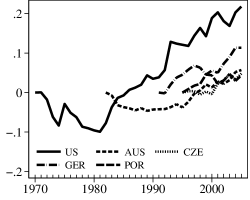
(a) (a) Increasing trend

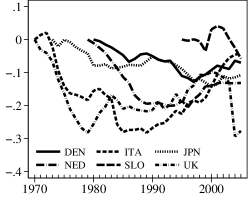
(b) (b) No clear trend

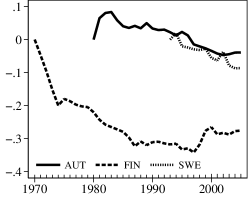
(c) (c) Decreasing trend

Notes: AUS: Australia, AUT: Austria, CZE: the Czech Republic, DEN: Denmark, FIN: Finland, GER: Germany, ITA: Italy, JPN: Japan, NED: the Netherlands, POR: Portugal, SLO: Slovenia, SWE: Sweden, UK: the United Kingdom, and US: the United States. All series are logged and normalized to zero in the initial year of observation.

4.2 Trends in factor prices and quantities

Trends in the skill premium vary across countries (Figure 1). The 14 countries are broadly divided into three groups for ease of visibility. The skill premium exhibits an increasing trend in five countries (Australia, the Czech Republic, Germany, Portugal, and the United States), no clear trend in six countries (Denmark, Italy, Japan, the Netherlands, Slovenia, and the United Kingdom), and a decreasing trend in three countries (Austria, Finland, and Sweden). As shown later, trends in the skill premium do not differ substantially across sectors.

Trends in the rental price of capital vary across capital types in the United States (Figure 2). The rental price of ICT capital fell steadily from the 1970s to the 2000s in the goods sector and from the mid-1980s to the 2000s in the service sector. Meanwhile, the rental price of non-ICT capital was roughly unchanged in the goods sector and slightly declined in the service sector from the 1970s to the 2000s. In all countries and sectors, the rental price of ICT capital declined much more than that of non-ICT capital (see Figures A1 and A2 in Appendix A.5 for countries other than the United States). The rate of decline in the rental price of ICT capital was greater for the goods sector than the service sector in the United States but not necessarily so in other countries.

Figure 2: Rental prices of ICT and non-ICT capital in the United States

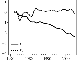
(a) (a) Goods sector

(b) (b) Service sector

Notes: The bold and dashed lines indicate the rental price of ICT capital ($r_{i}$) and the rental price of non-ICT capital ($r_{o}$), respectively. All series are logged and normalized to zero in the initial year.

Trends in capital and labor quantities vary across capital and labor types in the United States (Figure 3). The relative quantity of skilled to unskilled labor increased from the 1970s to the 2000s. The relative quantity of ICT equipment to skilled labor increased steadily and substantially after the mid-1970s, although the relative quantity of total capital equipment to skilled labor did not change substantially from the 1970s to the 2000s. The negative co-movement between the rental price and quantity of ICT equipment indicates technological change (Greenwood, Hercowitz, and Krusell, 1997). The capital–skill complementarity effect is proportional in magnitude to the ratio of ICT capital to skilled labor, while the relative labor quantity effect is proportional in magnitude to the ratio of skilled to unskilled labor. The observed trends in relative factor quantities suggest that the two effects would work in opposite directions. The same applies to all countries and sectors (see Figures A3 and A4 in Appendix A.5 for countries other than the United States). However, the magnitude and timing of changes in relative factor quantities vary greatly across countries and sectors. The rate of increase in the relative quantity of ICT equipment to skilled labor was greater in the goods sector than in the service sector in the United States but smaller in the goods sector than in the service sector in many other countries.

Figure 3: Relative factor quantities in the United States

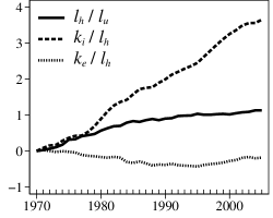
(a) (a) Goods sector

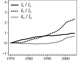
(b) (b) Service sector

Notes: The bold, dashed, and dotted lines indicate the ratios of skilled to unskilled labor ($\ell_{h}/\ell_{u}$), ICT capital to skilled labor ($k_{i}/\ell_{h}$), and capital equipment to skilled labor, ($k_{e}/\ell_{h}$), respectively. All series are logged and normalized to zero in the initial year.

5 Estimation

We start this section by specifying the estimating equations. We then discuss how we identify and estimate the parameters in the production function. We end this section by briefly describing how we decompose the sources of changes in the skill premium.

5.1 Econometric specifications

5.1.1 Factor-biased technological change

We incorporate factor-biased technological change, as well as capital–skill complementarity, in the production function. Technological change is said to be factor-biased (factor-neutral) if either or both of (neither) relative capital- and (nor) labor-augmenting technology changes over time. Technological change is said to be skill-biased if the ratio of skilled to unskilled labor-augmenting technology ($A_{h}/A_{u}$) increases over time. We can account for skill-biased technological change by allowing the share parameter $\lambda$ to increase over time. More flexibly, we can account for factor-biased technological change by allowing the two share parameters $\lambda$ and $\mu$ to change over time. The share parameters are specified to ensure that they lie between zero and one as follows:

$$\lambda_{cnt}=\frac{\exp\left(\sum_{\varsigma=0}^{S_{cn}^{\lambda}}\lambda_{\varsigma,cn}t^{\varsigma}\right)}{1+\exp\left(\sum_{\varsigma=0}^{S_{cn}^{\lambda}}\lambda_{\varsigma,cn}t^{\varsigma}\right)}\quad\text{and}\quad\mu_{cnt}=\frac{\exp\left(\sum_{\varsigma=0}^{S_{cn}^{\mu}}\mu_{\varsigma,cn}t^{\varsigma}\right)}{1+\exp\left(\sum_{\varsigma=0}^{S_{cn}^{\mu}}\mu_{\varsigma,cn}t^{\varsigma}\right)},$$ (11)

where $c$, $n$, and $t$ are the indices for countries, sectors, and years, respectively. Changes in the direction and magnitude of factor-biased technological change can be accounted for by adding higher-order trend terms. Differences in the speed and timing of factor-biased technological change can be accounted for by allowing the coefficients of trend terms to vary across countries and sectors. We choose the orders of polynomials ($S_{cn}^{\lambda}$ and $S_{cn}^{\mu}$) to fit the trends in the respective relative factor prices ($w_{h}/w_{u}$ and $w_{h}/r_{i}$) for each country and sector. This parameterization is sufficiently flexible to account for the trends in the relative factor prices for each country and sector, as shown below.

5.1.2 Wedge

Moreover, we allow the degree of competitiveness to vary across countries and sectors over time. The wedge can be decomposed as

$$\omega_{j,cnt}=\varpi_{j,cn}\varphi_{j,cnt}v_{j,cnt}^{\omega}\qquad\text{for}\enskip j\in\left\{h,u,i,o\right\},$$ (12)

where $\varpi$ is a time-invariant effect specific to each country and sector, $\varphi$ is a time-varying effect of wage-setting institutions, and $v^{\omega}$ is an idiosyncratic shock to the wedge. Any time-invariant country-specific factors can be eliminated by taking logs and differences over time, even though there are substantial and persistent differences in non-competitive and institutional factors across countries. Conceivably, however, the wedge may decrease as wage-setting institutions become less centralized. If the decrease in the wedge due to wage-setting institutions differs for skilled and unskilled labor, changes in the skill premium can be influenced by wage-setting institutions. We allow for this possibility in a robustness check by incorporating the collective bargaining coverage (i.e., the percentage of employees with the right to bargain) as a time-varying factor in the wedge. Information about the collective bargaining coverage can be obtained from OECD.Stat throughout the sample period.

5.1.3 Estimating equations

After substituting equations (11) and (12) into the marginal-rate-of-technical-substitution conditions (7) and (8) and taking differences over time, we obtain the following estimating equations:

$$\Delta\ln\left(\frac{w_{h,cnt}}{w_{u,cnt}}\right)=\sum_{\varsigma=1}^{S_{cn}^{\lambda}}\lambda_{\varsigma,cn}\Delta t^{\varsigma}-\frac{\sigma}{\rho}\Delta\ln\left[1+\exp\left(\sum_{\varsigma=0}^{S_{cn}^{\mu}}\mu_{\varsigma,cn}t^{\varsigma}\right)\right]\\ +\frac{\sigma-\rho}{\rho}\Delta\ln\left[\exp\left(\sum_{\varsigma=0}^{S_{cn}^{\mu}}\mu_{\varsigma,cn}t^{\varsigma}\right)\left(\frac{k_{i,cnt}}{\ell_{h,cnt}}\right)^{\rho}+1\right]-\left(1-\sigma\right)\Delta\ln\left(\frac{\ell_{h,cnt}}{\ell_{u,cnt}}\right)+\Delta\ln\left(\frac{\varphi_{h,cnt}}{\varphi_{u,cnt}}\right)+\Delta v_{1,cnt},$$ (13)

$$\Delta\ln\left(\frac{w_{h,cnt}}{r_{i,cnt}}\right)=-\sum_{\varsigma=1}^{S_{cn}^{\mu}}\mu_{\varsigma,cn}\Delta t^{\varsigma}-\left(1-\rho\right)\Delta\ln\left(\frac{\ell_{h,cnt}}{k_{i,cnt}}\right)+\Delta\ln\left(\frac{\varphi_{h,cnt}}{\varphi_{i,cnt}}\right)+\Delta v_{2,cnt},$$ (14)

where the error terms are $\Delta v_{1,cnt}=\Delta\ln(v_{h,cnt}^{\omega}/v_{u,cnt}^{\omega})$ and $\Delta v_{2,cnt}=\Delta\ln(v_{h,cnt}^{\omega}/v_{i,cnt}^{\omega})$. One of the substitution parameters ($\rho$) appears in both equations. The error terms are correlated across equations as the idiosyncratic shock $v_{h}^{\omega}$ is a component of the error terms in both equations. Thus, it is efficient to estimate the system of equations (13) and (14) jointly.

Two things could be worth mentioning. First, the error terms arise not from shocks to markup in the output market but from differences in shocks to the wedge across input markets. The error terms can also arise from changes in measurement errors in relative factor prices and quantities. Second, estimating equations (13) and (14) remain of the same form even if the wedge has time trends. In that case, the interpretation of decomposition results requires caution in that the relative factor-augmenting technology effect could be attributed in part to changes in the factor-specific wedge. However, following the convention in the literature, we use the term “technology” to refer to unobserved factors.

5.1.4 Instrumental variables

The substitution parameters ($\sigma$ and $\rho$) can be identified from variation in relative factor quantities across countries, sectors, and time. We allow for correlations between changes in factor quantities and idiosyncratic shocks, and estimate the substitution parameters using the shift–share instrument:

$$\Delta\ln z_{cnt}^{b}=\sum_{d\in\mathcal{D}_{n^{\prime}}}\frac{z_{dcn^{\prime}t_{0}}}{\sum_{d^{\prime}\in\mathcal{D}_{n^{\prime}}}z_{d^{\prime}cn^{\prime}t_{0}}}\Delta\ln\left(\sum_{c^{\prime}\neq c\in\mathcal{C}}z_{dc^{\prime}n^{\prime}t}\right)\qquad\text{for }z\in\left\{k_{i},\ell_{h},\ell_{u}\right\},$$ (15)

where $d$ is an index for subsectors (or equivalently industries), and $\mathcal{C}$ and $\mathcal{D}_{n}$ are the sets of countries and the set of subsectors in sector $n$, respectively. The shift–share instrument is the interaction between the growth rate of factors in each industry (shift), which measures global shocks to industries, and the lagged industry share of factors in each country (share), which measures local exposure to industry shocks. We construct the shift–share instrument using the data from the service (goods) sector to deal with the endogeneity of factor quantities in the goods (service) sector. The idea behind this is that a demand shock in one sector serves as a supply shifter in another sector to identify a demand curve (Oberfield and Raval, 2021). We evaluate the time-invariant measure of local industry shares at the initial year ($t=t_{0}$) to ensure the exogeneity of industry shares, and use the leave-one-out measure of global industry growth rates to ensure the exogeneity of industry shocks.

5.2 Generalized method of moments

We estimate the system of equations (13) and (14) jointly using the generalized method of moments (GMM). This approach is semi-parametric as it does not impose a distributional assumption on the error terms. We treat all capital and labor quantities as endogenous variables. Specifically, we use the change in the log ratio of the shift–share instruments, such as $\Delta\ln(\ell_{h}^{b}/\ell_{u}^{b})$ and $\Delta\ln(k_{i}^{b}/\ell_{h}^{b})$, as instrumental variables for the change in the log ratio of factor quantities, such as $\Delta\ln(\ell_{h}/\ell_{u})$ and $\Delta\ln(k_{i}/\ell_{h})$. We take five-year differences in the system of equations (13) and (14).

Let $\boldsymbol{\theta}$ denote the set of parameters to be estimated. The vector of parameters is $\boldsymbol{\theta}=(\sigma,\rho,\lambda_{1,cn},\ldots,\lambda_{S_{c}^{\lambda},cn},$ $\mu_{0,cn},\ldots,\mu_{S_{cn}^{\mu},cn})$. The GMM estimator $\widehat{\theta}$ is chosen to minimize the quadratic form:

$$\widehat{\boldsymbol{\theta}}=\arg\min_{\boldsymbol{\theta}}\enskip g_{N}\left(\boldsymbol{\theta}\right)^{\prime}\,\boldsymbol{W}_{N}\,g_{N}\left(\boldsymbol{\theta}\right),$$ (16)

where $g_{N}\left(\boldsymbol{\theta}\right)$ is a vector of the moment conditions, and $\boldsymbol{W}_{N}$ is a weighting matrix. Let $\boldsymbol{z}$ denote a vector of exogenous variables that include the instrumental variables and trend terms. The elements of $g_{N}\left(\theta\right)$ are $N^{-1}\sum_{c=1}^{14}\sum_{n=1}^{2}\sum_{t=1}^{T_{c}}\boldsymbol{z}_{m,cnt}v_{m,cnt}$ for $m=1,2$, where $T_{c}$ is the number of years used for estimation in country $c$, and $N$ is the sum of $T_{c}$ across countries multiplied by the number of sectors. The GMM estimator is consistent as the sample size ($N$) approaches infinity.

5.3 Decomposition

After estimating the production function, we decompose changes in the skill premium into the capital–skill complementarity effect associated with $k_{i}/\ell_{h}$, the relative labor quantity effect associated with $\ell_{h}/\ell_{u}$, and the relative factor-augmenting technology effect associated with $A_{h}/A_{u}$ or $A_{i}/A_{h}$ using equation (7). The three effects can be further decomposed into parts due to each factor and technology. The issue here is that the decomposition results generally depend on the order of decomposition as equation (7) is not additively linear in $k_{i}$, $\ell_{h}$, or $A_{i}/A_{h}$. The same issue arises when we decompose the sources of changes in the relative demand for skilled to unskilled labor using equation (10). We implement the Shapley decomposition to address the issue of path dependence (Shorrocks, 2013). Appendix A.6 provides a detailed description of the decomposition.

6 Results

We first present the estimates of the elasticities of substitution in production. We then discuss the sources and mechanisms of changes in the skill premium for each country and sector and of the differences in changes in the skill premium across countries.

6.1 Production function estimates

6.1.1 Capital–Skill complementarity

The four-factor production function involves two substitution parameters ($\sigma$ and $\rho$) and two share parameters ($\lambda$ and $\mu$). Table 1 presents the estimates of the substitution parameters. Although we focus on the results when we allow technological change to be factor-biased, we also report the results when we assume technological change to be factor-neutral for reference. The estimates of the substitution parameters are greater in absolute value in the former case than in the latter case. Subsequent figures present the estimates of the share parameters, which consist of higher-order trend terms and their country- and sector-specific coefficients, in the form of the relative factor-augmenting technology effect.

Table 1: Production function estimates

$\sigma$		$\rho$
Factor-biased
technological change
0.	888	–0.	162
(0.	029)	(0.	051)
[0.	026]	[0.	057]
Factor-neutral
technological change
0.	642	–0.	053
(0.	248)	(0.	047)
[0.	130]	[0.	053]

Notes: Standard errors in parentheses are clustered at the country-sector level, and those in square brackets are Newey–West adjusted with the optimal lag length (Newey and West, 1994).

Our results indicate that ICT equipment is much more complementary to skilled labor than unskilled labor even in the presence of factor-biased technological change, which strongly confirms the ICT capital–skill complementarity hypothesis (i.e., $\sigma>\rho$). The estimate of $\rho$, which governs the degree of substitution between $k_{i}$ and $\ell_{h}$, is close to that in Krusell et al. (2000), while the estimate of $\sigma$, which governs the degree of substitution between the $k_{i}$-$\ell_{h}$ composite and $\ell_{u}$, is greater than that in Krusell et al. (2000). Consequently, the estimated difference between the two substitution parameters ($\sigma-\rho$), to which the capital–skill complementarity effect is proportional, is slightly greater here. Polgreen and Silos (2008) show that the estimate of $\sigma$ becomes greater when using data from the National Income and Product Accounts (NIPA) than when using the data in Krusell et al. (2000). Our estimate of $\sigma$ is close to what Polgreen and Silos (2008) obtain from the NIPA data.

6.1.2 Robustness checks

We examine whether the results presented above are robust to the influence of international trade and wage-setting institutions. Table 2 presents the extent to which the estimates of the substitution parameters vary when splitting the sample by sector and when controlling for the collective bargaining coverage.

The first, second, and third rows of Table 2 report the estimated substitution parameters for all, goods, and service sectors, respectively. The estimates of $\sigma$ and $\rho$ are similar for the goods and service sectors. In addition, the estimated difference between the two substitution parameters ($\sigma-\rho$), to which the capital–skill complementarity effect is proportional, is almost the same for the goods and service sectors. The ICT capital–skill complementarity hypothesis appears to hold irrespective of the influence of international trade.

The last row of Table 2 indicates that the estimated substitution parameters remain almost unchanged even after allowing the wedge to vary with the degree of centralized wage bargaining. The coefficient of the collective bargaining coverage is insignificant, indicating that the skill premium is not associated with the collective bargaining coverage, conditional on the capital–skill complementarity effect, relative labor quantity effect, and relative factor-augmenting technology effect.

Table 2: Robustness checks

	$\sigma$	$\rho$
All sectors	0.888	–0.162
	(0.029)	(0.051)
Goods sector	0.847	–0.114
	(0.036)	(0.113)
Service sector	0.889	–0.123
	(0.032)	(0.043)
Collective bargaining coverage	0.873	–0.119
	(0.025)	(0.045)

Notes: Standard errors in parentheses are clustered at the country-sector level.

6.1.3 Morishima elasticities

Table 3 presents the estimates of the Morishima elasticities of substitution among ICT equipment, skilled labor, and unskilled labor. ICT equipment is much more substitutable with unskilled labor than skilled labor, while skilled labor is more substitutable with unskilled labor than ICT equipment. The former result confirms the presence of capital–skill complementarity. The latter result implies that the degree of labor–labor substitution is greater than that of capital–labor substitution. The Morishima elasticities are asymmetric. The estimated elasticity of $\ell_{u}$ with respect to $r_{i}$ is smaller than that of $k_{i}$ with respect to $w_{u}$.

Table 3: Morishima elasticities of substitution

	$k_{i}$		$\ell_{h}$		$\ell_{u}$
$k_{i}$			0.	860	8.	943
			(0.	038)	(2.	303)
$\ell_{h}$	0.	860			8.	943
	(0.	038)			(2.	303)
$\ell_{u}$	2.	324	7.	479
	(0.	629)	(2.	004)

Notes: Elasticities are evaluated at the sample means. Standard errors in parentheses are clustered at the country-sector level.

Figure 4: Actual and predicted skill premium ($w_{h}/w_{u}$) in the goods sector

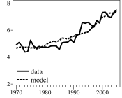
(a) (a) United States

(b) (b) Australia

(c) (c) Austria

(d) (d) Czech Republic

(e) (e) Denmark

(f) (f) Finland

(g) (g) Germany

(h) (h) Italy

(i) (i) Japan

(j) (j) Netherlands

(k) (k) Portugal

(l) (l) Slovenia

(m) (m) Sweden

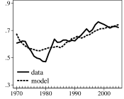
(n) (n) United Kingdom

Notes: The bold and dashed lines indicate the actual and predicted values, respectively. All series are logged.

Figure 5: Actual and predicted skill premium ($w_{h}/w_{u}$) in the service sector

(a) (a) United States

(b) (b) Australia

(c) (c) Austria

(d) (d) Czech Republic

(e) (e) Denmark

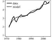
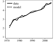
(f) (f) Finland

(g) (g) Germany

(h) (h) Italy

(i) (i) Japan

(j) (j) Netherlands

(k) (k) Portugal

(l) (l) Slovenia

(m) (m) Sweden

(n) (n) United Kingdom

Notes: The bold and dashed lines indicate the actual and predicted values, respectively. All series are logged.

Figure 6: Actual and predicted ratio of the wages of skilled labor to the rental price of ICT capital ($w_{h}/r_{i}$) in the goods sector

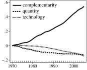
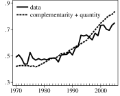
(a) (a) United States

(b) (b) Australia

(c) (c) Austria

(d) (d) Czech Republic

(e) (e) Denmark

(f) (f) Finland

(g) (g) Germany

(h) (h) Italy

(i) (i) Japan

(j) (j) Netherlands

(k) (k) Portugal

(l) (l) Slovenia

(m) (m) Sweden

(n) (n) United Kingdom

Notes: The bold and dashed lines indicate the actual and predicted values, respectively. All series are logged.

Figure 7: Actual and predicted ratio of the wages of skilled labor to the rental price of ICT capital ($w_{h}/r_{i}$) in the service sector

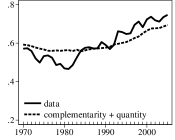
(a) (a) United States

(b) (b) Australia

(c) (c) Austria

(d) (d) Czech Republic

(e) (e) Denmark

(f) (f) Finland

(g) (g) Germany

(h) (h) Italy

(i) (i) Japan

(j) (j) Netherlands

(k) (k) Portugal

(l) (l) Slovenia

(m) (m) Sweden

(n) (n) United Kingdom

Notes: The bold and dashed lines indicate the actual and predicted values, respectively. All series are logged.

6.2 Skill premium

6.2.1 Accounting for changes in the skill premium

Changes in the skill premium over a few decades can be explained well by the production function with capital–skill complementarity and factor-augmenting technology for all countries and sectors. Figures 4 and 5 show that the actual values of the skill premium ($w_{h}/w_{u}$) almost overlap the predicted values from equation (7) in the goods and service sectors of all countries. Figures 6 and 7 show that the actual values of the ratio of skilled wages to the rental price of ICT capital ($w_{h}/r_{i}$) almost overlap the predicted values from equation (8) in the goods and service sectors of all countries. The orders of the trend polynomials in equation (11) are chosen to fit the data for each country and sector.

6.2.2 Decomposition of changes in the skill premium

We decompose changes in the skill premium into the capital–skill complementarity effect, relative labor quantity effect, and relative factor-augmenting technology effect. Figures 8 and 9 show the direction and magnitude of the three effects in the goods and service sectors of 14 OECD countries. The rise in the skill premium from the 1980s to the 2000s in the goods and service sectors of the United States is attributable mostly to the capital–skill complementarity effect, while the decline in the skill premium in the 1970s in the goods and service sectors of the United States is attributable to the relative labor quantity effect and relative factor-augmenting technology effect. Similarly, the increase in the skill premium in the service sector of Germany, the Czech Republic, and Portugal is attributable entirely to the capital–skill complementarity effect. Perhaps surprisingly, the relative factor-augmenting technology effect is not needed to account for the increasing trend in the skill premium in these countries. The capital–skill complementarity effect associated with a rise in ICT equipment is large enough to account for a rise in the skill premium in almost all countries. The increase in the skill premium in the goods sector of Germany and the United Kingdom is, however, attributable mainly to the relative factor-augmenting technology effect.

Figure 8: Decomposition of changes in the skill premium in the goods sector

(a) (a) United States

(b) (b) Australia

(c) (c) Austria

(d) (d) Czech Republic

(e) (e) Denmark

(f) (f) Finland

(g) (g) Germany

(h) (h) Italy

(i) (i) Japan

(j) (j) Netherlands

(k) (k) Portugal

(l) (l) Slovenia

(m) (m) Sweden

(n) (n) United Kingdom

Notes: The bold, dashed, and dotted lines indicate the capital–skill complementarity effect, relative labor quantity effect, and relative factor-augmenting technology effect, respectively. All series are logged and normalized to zero in the initial year.

Figure 9: Decomposition of changes in the skill premium in the service sector

(a) (a) United States

(b) (b) Australia

(c) (c) Austria

(d) (d) Czech Republic

(e) (e) Denmark

(f) (f) Finland

(g) (g) Germany

(h) (h) Italy

(i) (i) Japan

(j) (j) Netherlands

(k) (k) Portugal

(l) (l) Slovenia

(m) (m) Sweden

(n) (n) United Kingdom

Notes: The bold, dashed, and dotted lines indicate the capital–skill complementarity effect, relative labor quantity effect, and relative factor-augmenting technology effect, respectively. All series are logged and normalized to zero in the initial year.

Figure 10: Trends in the skill premium attributable to observed factors in the goods sector

(a) (a) United States

(b) (b) Australia

(c) (c) Austria

(d) (d) Czech Republic

(e) (e) Denmark

(f) (f) Finland

(g) (g) Germany

(h) (h) Italy

(i) (i) Japan

(j) (j) Netherlands

(k) (k) Portugal

(l) (l) Slovenia

(m) (m) Sweden

(n) (n) United Kingdom

Notes: The bold line indicates the actual values. The dashed line indicates the sum of the capital–skill complementarity effect and relative labor quantity effect. The relative factor-augmenting technology effect is held constant at the sample mean.

Figure 11: Trends in the skill premium attributable to observed factors the service sector

(a) (a) United States

(b) (b) Australia

(c) (c) Austria

(d) (d) Czech Republic

(e) (e) Denmark

(f) (f) Finland

(g) (g) Germany

(h) (h) Italy

(i) (i) Japan

(j) (j) Netherlands

(k) (k) Portugal

(l) (l) Slovenia

(m) (m) Sweden

(n) (n) United Kingdom

Notes: The bold line indicates the actual values. The dashed line indicates the sum of the capital–skill complementarity effect and relative labor quantity effect. The relative factor-augmenting technology effect is held constant at the sample mean.

It is common in all countries that the capital–skill complementarity effect contributes to widening the skill premium, while the relative labor quantity effect contributes to narrowing it. The magnitude of the two effects differs across countries and years, however. The capital–skill complementarity effect was particularly large in Denmark, Finland, and the United States, while the relative labor quantity effect was particularly large in the United Kingdom. The capital–skill complementarity effect was greater for the goods sector than the service sector in the majority of countries, while the relative labor quantity effect was similar for the goods and service sectors in most countries. The relative factor-augmenting technology effect differs in direction, as well as magnitude, across countries, sectors, and years.

Trends in the skill premium can be attributed to observed factors in the majority of countries. Figures 10 and 11 show the trends in the skill premium attributable to observed factors, which are calculated as the sum of the capital–skill complementarity effect and relative labor quantity effect, along with the actual trends in the goods and service sectors. The skill premium trends attributable to observed factors line up with the actual trends in the goods sector of eight countries (Australia, the Czech Republic, Italy, Japan, the Netherlands, Slovenia, Sweden, and the United States) and the service sector of nine countries (Australia, Austria, the Czech Republic, Germany, Portugal, Slovenia, Sweden, the United Kingdom, and the United States). Among these countries, the skill premium has an increasing trend in the goods (service) sector of the United States (the Czech Republic, Germany, Portugal, and the United States); no clear trend in the goods (service) sector of Australia, the Czech Republic, the Netherlands, and Slovenia (Australia, Austria, Slovenia, and the United Kingdom); and a decreasing trend in the goods (service) sector of Italy, Japan, and Sweden (Sweden). Trends in the skill premium attributable to observed factors also align partially with the actual trends in the service sector of three countries (Denmark, Japan, and the Netherlands). These results indicate that changes in the skill premium can be interpreted as a consequence of the capital–skill complementarity effect and relative labor quantity effect. Meanwhile, the skill premium trends attributable to observed factors do not align with the actual trends in the goods sector of six countries (Austria, Denmark, Finland, Germany, Portugal, and the United Kingdom) and the service sector of two countries (Finland and Italy). Unobserved factors cannot be disregarded as determinants of changes in the skill premium in these countries.

6.2.3 Decomposition of international differences in changes in the skill premium

We examine the extent to which international differences in changes in the skill premium are attributed to specific observed or unobserved factors. Table 4 presents the decomposition results of the differences in changes in the skill premium compared to the United States. The first two columns report the actual and predicted differences in changes in the skill premium from the first year of observation to the year 2005 between the United States and other countries. Almost all the values in the first column are positive, meaning that the rate of increase in the skill premium was greater in the United States than in other countries. The next five columns report the parts attributable to ICT equipment, skilled labor, unskilled labor, the ratio of skilled to unskilled labor-augmenting technology, and the ratio of ICT capital- to skilled labor-augmenting technology, respectively.

Table 4: Decomposition of the differences in changes in the skill premium compared to the United States

Countries		$\ln(w_{h}/w_{u})$					$k_{i}$		$\ell_{h}$		$\ell_{u}$		$A_{h}/A_{u}$		$A_{i}/A_{h}$
		Data		Model
AUS		0.	225	0.	182		0.	303	0.	050	–0.	005	0.	617	–0.	783
AUT		0.	162	0.	179		–0.	501	–0.	002	0.	030	–0.	666	1.	318
CZE		0.	084	0.	119		0.	141	–0.	006	0.	013	0.	348	–0.	377
DEN		0.	452	0.	447		0.	062	0.	050	0.	018	0.	727	–0.	410
FIN		0.	551	0.	499		–0.	318	–0.	080	0.	074	0.	179	0.	643
GER		–0.	011	–0.	014		0.	237	–0.	080	0.	041	0.	297	–0.	509
ITA		0.	503	0.	476		0.	588	–0.	169	0.	038	1.	145	–1.	125
JPN		0.	406	0.	357		0.	624	–0.	155	0.	049	0.	927	–1.	089
NED		0.	332	0.	378		0.	076	0.	261	0.	001	1.	166	–1.	126
POR		0.	117	0.	254		0.	052	0.	040	0.	002	0.	537	–0.	377
SLO		0.	133	0.	212		0.	201	0.	020	0.	019	0.	351	–0.	379
SWE		0.	195	0.	256		0.	191	0.	097	0.	004	0.	408	–0.	444
UK		0.	147	0.	204		0.	566	0.	049	0.	073	0.	824	–1.	309

(a) Goods sector

Countries		$\ln(w_{h}/w_{u})$					$k_{i}$		$\ell_{h}$		$\ell_{u}$		$A_{h}/A_{u}$		$A_{i}/A_{h}$
		Data		Model
AUS		0.	257	0.	193		0.	056	0.	133	–0.	004	0.	254	–0.	246
AUT		0.	289	0.	280		0.	124	–0.	004	0.	005	0.	421	–0.	265
CZE		0.	044	0.	027		0.	059	–0.	023	0.	007	0.	095	–0.	111
DEN		0.	313	0.	243		0.	032	–0.	001	0.	018	0.	459	–0.	265
FIN		0.	356	0.	297		–0.	458	0.	047	0.	020	–0.	013	0.	701
GER		0.	094	0.	084		0.	107	–0.	042	0.	011	0.	162	–0.	154
ITA		–0.	007	0.	014		0.	129	0.	002	–0.	012	0.	335	–0.	440
JPN		0.	352	0.	355		0.	082	–0.	008	0.	035	0.	575	–0.	329
NED		0.	339	0.	307		0.	128	0.	037	–0.	005	0.	422	–0.	276
POR		–0.	002	–0.	017		0.	021	–0.	011	–0.	011	0.	095	–0.	111
SLO		0.	173	0.	063		0.	061	0.	015	0.	003	0.	095	–0.	111
SWE		0.	177	0.	178		0.	089	0.	027	0.	016	0.	178	–0.	133
UK		0.	491	0.	470		0.	183	0.	187	0.	007	0.	549	–0.	456

(b) Service sector

Notes: The differences in changes in the skill premium between the United States and other countries are decomposed into the parts attributable to ICT capital ($k_{i}$), skilled labor ($\ell_{h}$), unskilled labor ($\ell_{u}$), the ratio of skilled to unskilled labor-augmenting technology ($A_{h}/A_{u}$), and the ratio of ICT capital- to skilled labor-augmenting technology ($A_{i}/A_{h}$).

Cross-country differences in changes in the skill premium can be explained by specific capital and labor quantities in the majority of countries. The main factors accounting for the differences are ICT equipment and skilled labor in the goods (service) sector of the Netherlands, Portugal, and Sweden (Australia and the United Kingdom), and ICT equipment in the goods (service) sector of Australia, Italy, Japan, and Slovenia (Austria, the Czech Republic, Germany, Japan, the Netherlands, Slovenia, and Sweden). The differences in changes in the skill premium compared to the United States are attributable at least in part to ICT equipment in almost all countries. This result reflects the fact that the contribution of ICT equipment to changes in the skill premium was large in the United States for two reasons. First, the rate of increase in ICT equipment ($k_{i}$) was large in the United States. Second, the rate of increase in the ratio of ICT capital- to skilled labor-augmenting technology ($A_{i}/A_{h}$) was small in the United States. The contribution of ICT equipment to changes in the skill premium increases with a decline in $A_{i}/A_{h}$ as the cross-derivative of the skill premium with respect to $k_{i}$ and $A_{i}/A_{h}$ is negative for $\sigma>\rho$ and $\rho<0$ in equation (7).

Not surprisingly, however, international differences in changes in the skill premium cannot be explained solely by observed factors. Especially in Finland, where the capital–skill complementarity effect is greater than or at least comparable to that in the United States, the differences in changes in the skill premium compared to the United States are attributed mainly to the relative factor-augmenting technology effect. The relative factor-augmenting technology effect can be decomposed into two parts, one attributable to $A_{h}/A_{u}$ and the other attributable to $A_{i}/A_{h}$, the former of which is typically referred to as skill-biased technological change when it increases over time. The sixth and seventh columns show that the two effects work in opposite directions in all countries. The relative factor-augmenting technology effect is negligible in the United States because the two effects are canceled out. Interestingly, skill-biased technological change is greater in the United States than in other countries.

6.2.4 Decomposition of changes in relative labor demand

We measure the contribution of factor prices to changes in the relative demand for skilled to unskilled labor. Table 5 presents the decomposition results of changes in relative labor demand into factor prices and relative factor-augmenting technology. The first two columns report the actual and predicted changes in relative labor quantity from the first year of observation till the year 2005 for each country. The changes predicted from the factor demand function fit reasonably well with the actual data, even though the parameters are not chosen to account for changes in the relative demand for skilled to unskilled labor.

The next five columns report the parts attributable to the rental price of ICT capital, the wages of skilled and unskilled labor, and two types of relative factor-augmenting technology, respectively. As seen in Figures 3, A3, and A4, the relative quantity of skilled to unskilled labor increased in all countries. On the one hand, as the relative demand for skilled labor should decline with a rise in the relative wages of skilled labor, a rise in relative labor quantity is not attributable to relative wages in countries such as the United States that saw a rise in the skill premium. On the other hand, as the relative demand for skilled labor should increase with a fall in the rental price of ICT capital in the presence of capital–skill complementarity, a rise in relative labor quantity may be attributable to the rental price. As seen in Figures 2, A1, and A2, the rental price of ICT capital fell in all countries. An important question here is the extent to which a rise in relative labor quantity is attributable to a fall in the rental price of ICT capital. The results indicate that a fall in the rental price of ICT capital is large enough to account for a rise in relative labor quantity in the goods and service sectors of the United States. The same applies to the goods or service sector of almost all countries.

Table 5: Decomposition of changes in relative labor demand

Countries		$\ln(\ell_{h}/\ell_{u})$					$r_{i}$		$w_{h}$		$w_{u}$		$A_{h}/A_{u}$		$A_{h}/A_{i}$
		Data		Model
US		1.	066	1.	207		2.	538	–4.	600	2.	795	8.	371	–7.	897
AUS		0.	990	0.	997		0.	591	–1.	043	0.	687	0.	762	0.	000
AUT		0.	688	1.	041		4.	053	–4.	906	5.	122	12.	668	–15.	896
CZE		0.	202	0.	626		0.	535	–2.	801	2.	892	0.	000	0.	000
DEN		1.	076	0.	982		2.	222	–1.	444	3.	150	0.	215	–3.	161
FIN		1.	222	1.	250		2.	846	–6.	969	9.	826	7.	464	–11.	916
GER		0.	212	0.	270		0.	302	–3.	051	1.	724	1.	295	0.	000
ITA		0.	966	1.	361		0.	576	–5.	448	7.	457	–1.	224	0.	000
JPN		1.	192	1.	180		0.	104	–9.	961	10.	901	–0.	126	0.	262
NED		1.	508	1.	418		2.	313	–1.	931	2.	728	–3.	498	1.	806
POR		0.	489	–0.	169		0.	633	–0.	408	0.	627	–1.	021	0.	000
SLO		0.	517	0.	552		0.	001	–1.	544	2.	104	–0.	020	0.	011
SWE		0.	789	1.	214		0.	001	–3.	356	4.	568	0.	000	0.	000
UK		2.	269	2.	632		0.	366	–7.	785	7.	058	2.	413	0.	580

(a) Goods sector

Countries		$\ln(\ell_{h}/\ell_{u})$					$r_{i}$		$w_{h}$		$w_{u}$		$A_{h}/A_{u}$		$A_{h}/A_{i}$
		Data		Model
US		0.	854	0.	875		1.	156	–3.	228	1.	800	3.	656	–2.	509
AUS		1.	302	1.	477		0.	870	–1.	584	1.	625	0.	566	0.	000
AUT		0.	681	0.	196		0.	745	–0.	530	0.	653	–0.	673	0.	000
CZE		0.	188	0.	062		0.	523	–1.	852	1.	391	0.	000	0.	000
DEN		0.	834	0.	863		1.	484	–1.	815	2.	210	–1.	016	0.	000
FIN		0.	943	0.	895		2.	732	–0.	295	1.	338	4.	155	–7.	036
GER		0.	103	–0.	108		0.	490	–1.	620	1.	021	0.	000	0.	000
ITA		1.	035	1.	764		1.	207	–0.	493	–0.	677	0.	651	1.	076
JPN		1.	192	1.	038		1.	145	–4.	304	5.	699	–1.	502	0.	000
NED		0.	925	0.	809		0.	646	0.	475	0.	256	–0.	569	0.	000
POR		0.	167	–0.	156		0.	557	–0.	110	–0.	604	0.	000	0.	000
SLO		0.	336	0.	881		0.	376	–0.	738	1.	243	0.	000	0.	000
SWE		0.	529	0.	412		0.	203	–0.	765	1.	357	–0.	382	0.	000
UK		2.	197	2.	752		0.	399	–0.	018	2.	438	–0.	173	0.	106

(b) Service sector

Notes: Changes in the relative demand for skilled to unskilled labor are decomposed into the parts attributable to the rental price of ICT capital ($r_{i}$), the wages of skilled labor ($w_{h}$), the wages of unskilled labor ($w_{u}$), the ratio of skilled to unskilled labor-augmenting technology ($A_{h}/A_{u}$), and the ratio of ICT capital- to skilled labor-augmenting technology ($A_{i}/A_{h}$).

6.2.5 Impact of higher education expansion

The increased use of ICT results in a widening of the wage gap between skilled and unskilled workers, while it would result in an increase in production efficiency. One way to prevent a rise in the skill wage gap is to raise the supply of skilled labor by expanding access to tertiary education. When ICT equipment is more complementary to skilled labor than unskilled labor, such a policy is more effective in reducing the skill premium as it not only raises the relative labor quantity effect but also reduces the capital–skill complementarity effect. We end our analysis by measuring the quantitative importance of capital–skill complementarity in the evaluation for the impact of higher education expansion.

Table 6: Contribution of an increase in skilled labor to reducing the skill premium

Countries		$\ell_{h}$			$\ell_{h}^{CSC}$		$\ell_{h}^{RLQ}$		$(\ell_{h}^{CSC}+\ell_{h}^{RLQ})/\ell_{h}^{RLQ}$
US		–0.	274		–0.	154	–0.	121	2.27
AUS		–0.	170		–0.	051	–0.	118	1.43
AUT		–0.	127		–0.	087	–0.	040	3.19
CZE		–0.	007		–0.	002	–0.	005	1.51
DEN		–0.	179		–0.	085	–0.	095	1.90
FIN		–0.	195		–0.	123	–0.	072	2.72
GER		0.	025		0.	008	0.	017	1.47
ITA		–0.	105		–0.	031	–0.	074	1.43
JPN		–0.	082		–0.	009	–0.	073	1.12
NED		–0.	404		–0.	248	–0.	156	2.59
POR		–0.	053		–0.	020	–0.	034	1.59
SLO		–0.	034		0.	000	–0.	033	1.00
SWE		–0.	133		–0.	041	–0.	092	1.45
UK		–0.	323		–0.	074	–0.	249	1.30

(a) Goods sector

Countries		$\ell_{h}$			$\ell_{h}^{CSC}$		$\ell_{h}^{RLQ}$		$(\ell_{h}^{CSC}+\ell_{h}^{RLQ})/\ell_{h}^{RLQ}$
US		–0.	275		–0.	120	–0.	155	1.77
AUS		–0.	284		–0.	096	–0.	189	1.51
AUT		–0.	166		–0.	057	–0.	109	1.52
CZE		–0.	033		–0.	011	–0.	022	1.49
DEN		–0.	169		–0.	056	–0.	113	1.49
FIN		–0.	322		–0.	183	–0.	139	2.32
GER		–0.	036		–0.	011	–0.	025	1.45
ITA		–0.	277		–0.	098	–0.	179	1.55
JPN		–0.	233		–0.	089	–0.	144	1.62
NED		–0.	213		–0.	068	–0.	145	1.47
POR		–0.	045		–0.	015	–0.	030	1.51
SLO		–0.	071		–0.	025	–0.	047	1.53
SWE		–0.	100		–0.	034	–0.	066	1.52
UK		–0.	462		–0.	114	–0.	348	1.33

(b) Service sector

Notes: Changes in the log of the skill premium attributable to skilled labor ($\ell_{h}$) are decomposed into the part attributable to the capital–skill complementarity effect ($\ell_{h}^{CSC}$) and the part attributable to the relative labor quantity effect ($\ell_{h}^{RLQ}$).

Table 6 decomposes the contribution of skilled labor to changes in the skill premium into the contribution through the capital–skill complementarity effect and the contribution through the relative labor quantity effect. The first column reports the extent to which a rise in skilled labor had an effect on changes in the log of the skill premium from the first year of observation to the year 2005 for each country. The second and third columns report the parts attributable to the capital–skill complementarity effect and the relative labor quantity effect, respectively. The contribution through the capital–skill complementarity effect is not negligible in all countries and is comparable to or greater than the contribution through the relative labor quantity effect in a few countries such as Finland and the United States. The fourth column reports the ratio of the impact of skilled labor on the skill premium in the presence and absence of capital–skill complementarity. The results imply that the impact of higher education expansion is 1.78 (1.58) times greater for the goods (service) sector on average when the capital–skill complementarity effect is taken into account than when it is not.

7 Conclusion

This study examines the sources and mechanisms of changes in the skill premium for each country and sector and the differences in such changes across countries. We estimate a sector-level production function extended to allow for capital–skill complementarity and factor-biased technological change using cross-country and cross-industry panel data. We then decompose changes in the skill premium into the capital–skill complementarity effect, relative labor quantity effect, and relative factor-augmenting technology effect in the goods and service sectors of 14 OECD countries from the 1970s to the 2000s. The capital–skill complementarity effect and relative labor quantity effect arise from changes in the composition of capital and labor in production, while the relative factor-augmenting technology effect arises from other factors such as unobserved factor-biased technological change. Our results indicate that most of the changes in the skill premium can be accounted for by the capital–skill complementarity effect and relative labor quantity effect in the majority of countries when ICT equipment is distinguished from non-ICT capital. A large part of the differences in changes in the skill premium among those countries can be explained by ICT equipment, skilled labor, and unskilled labor.

Consequently, we show that whether the skill premium would eventually increase or decrease depends on the outcome of the race between demand shifts driven by the expansion of ICT and supply shifts driven by the expansion of access to higher education. On the one hand, the skill premium can increase due to the capital–skill complementarity effect, the magnitude of which is proportional to the rate of increase in the ratio of ICT equipment to skilled labor. On the other hand, the skill premium can decrease due to the relative labor quantity effect, the magnitude of which is proportional to the rate of increase in the ratio of skilled to unskilled labor. The expansion of ICT can result in a widening of the wage gap between skilled and unskilled workers, although it can yield significant benefits to the economy as a whole. Our results imply that the expansion of access to higher education is effective in preventing a rise in the skill wage gap not only by raising the relative labor quantity effect but also by reducing the capital–skill complementarity effect.

Appendix A Appendix

A.1 Derivation of the first-order conditions

We consider the profit maximization problem of a representative firm in competitive markets. Production technology is given by

$$y_{t}=f\left(\boldsymbol{k}_{t},\boldsymbol{\ell}_{t};A_{t}\right),$$ (17)

where $\boldsymbol{k}_{t}$ and $\boldsymbol{\ell}_{t}$ are the vectors of capital and labor inputs in period $t$, that is, $\boldsymbol{k}_{t}=(k_{1t},\ldots,k_{jt},\ldots,k_{J_{k}t})$ and $\boldsymbol{\ell}_{t}=(\ell_{1t},\ldots,\ell_{jt},\ldots,\ell_{J_{\ell}t})$, respectively.

Let $\chi$ denote investment and $q$ the price of investment. The Bellman equation of the problem can be written as

$$V\left(\boldsymbol{k}_{t}\right)=\max_{k_{j,t+1},\ell_{jt},\chi_{jt}}\left\{y_{t}-\sum_{j=1}^{J_{k}}q_{jt}\chi_{jt}-\sum_{j=1}^{J_{\ell}}w_{jt}\ell_{jt}+\beta_{t+1}\mathbb{E}_{t}\left[V\left(\boldsymbol{k}_{t+1}\right)\right]\right\}$$ (18)

subject to the law of motion of capital:

$$k_{j,t+1}=\left(1-\delta_{j}\right)k_{jt}+\chi_{jt}.$$ (19)

The discount factor is given by $\beta_{t}=1/(1+i_{t})$, where $i$ is the interest rate.

The first-order condition with respect to $k_{j,t+1}$ is

$$q_{jt}=\beta_{t+1}\mathbb{E}_{t}\left[\frac{\partial V_{t+1}}{\partial k_{j,t+1}}\right].$$ (20)

From the envelope theorem,

$$\frac{\partial V_{t}}{\partial k_{jt}}=\frac{\partial f_{t}}{\partial k_{jt}}+q_{jt}\left(1-\delta_{j}\right).$$ (21)

Assume that the firm makes its investment decisions with knowledge of $A_{t+1}$ and $q_{j,t+1}$. The first-order condition can be rewritten as

$$\frac{\partial f_{t+1}}{\partial k_{j,t+1}}=\delta_{j}q_{j,t+1}+i_{t+1}q_{jt}-\left(q_{j,t+1}-q_{jt}\right)\equiv r_{j,t+1},$$ (22)

where $r_{jt}$ is referred to as the rental price of capital or the user cost of capital. The first-order condition with respect to $\ell_{jt}$ is given by

$$\frac{\partial f_{t}}{\partial\ell_{jt}}=w_{jt}.$$ (23)

Equations for the no-arbitrage condition for capital equipment and structure and for the wage-bill ratio in Krusell et al. (2000) can be obtained from equations (22) and (23), respectively. In the main text, we allow for the deviation from the profit-maximizing conditions in competitive markets.

A.2 Factor demand and substitution

The factor demand functions can be derived from the four-factor production function (2) as

$$\ell_{h} = y\left[\frac{\left(1-\alpha\right)r_{o}}{\omega_{o}\alpha}\right]^{\alpha}\left(\frac{\omega_{h}}{w_{h}}\right)^{\frac{1}{1-\rho}}A_{h}^{\frac{\rho}{1-\rho}}B^{-\frac{\sigma-\rho}{\left(1-\rho\right)\left(1-\sigma\right)}}C^{\frac{1-\alpha+\alpha\sigma}{1-\sigma}},$$ (24)

$$k_{i} = y\left[\frac{\left(1-\alpha\right)r_{o}}{\omega_{o}\alpha}\right]^{\alpha}\left(\frac{\omega_{i}}{r_{i}}\right)^{\frac{1}{1-\rho}}A_{i}^{\frac{\rho}{1-\rho}}B^{-\frac{\sigma-\rho}{\left(1-\rho\right)\left(1-\sigma\right)}}C^{\frac{1-\alpha+\alpha\sigma}{1-\sigma}},$$ (25)

$$\ell_{u} = y\left[\frac{\left(1-\alpha\right)r_{o}}{\omega_{o}\alpha}\right]^{\alpha}\left(\frac{\omega_{u}}{w_{u}}\right)^{\frac{1}{1-\sigma}}A_{u}^{\frac{\sigma}{1-\sigma}}C^{\frac{1-\alpha+\alpha\sigma}{1-\sigma}},$$ (26)

$$k_{o} = y\left[\frac{\left(1-\alpha\right)r_{o}}{\omega_{o}\alpha}\right]^{\alpha-1}C^{1-\alpha},$$ (27)

where

$$B = \left(\omega_{i}^{\frac{\rho}{1-\rho}}A_{i}^{\frac{\rho}{1-\rho}}r_{i}^{-\frac{\rho}{1-\rho}}+\omega_{h}^{\frac{\rho}{1-\rho}}A_{h}^{\frac{\rho}{1-\rho}}w_{h}^{-\frac{\rho}{1-\rho}}\right)^{-\frac{1-\rho}{\rho}},$$ (28)

$$C = \left(B^{-\frac{\sigma}{1-\sigma}}+\omega_{u}^{\frac{\sigma}{1-\sigma}}A_{u}^{\frac{\sigma}{1-\sigma}}w_{u}^{-\frac{\sigma}{1-\sigma}}\right)^{-\frac{1-\sigma}{\sigma}}.$$ (29)

The relative demand for skilled to unskilled labor can be written in logs using equations (24) and (26) as

$$\ln\left(\frac{\ell_{h}}{\ell_{u}}\right) = -\frac{1}{1-\rho}\ln w_{h}+\frac{1}{1-\sigma}\ln w_{u}-\frac{\sigma-\rho}{\left(1-\sigma\right)\left(1-\rho\right)}\ln D$$ (30)

$$+\frac{1}{1-\sigma}\left[\sigma\ln\left(\frac{A_{h}}{A_{u}}\right)+\ln\left(\frac{\omega_{h}}{\omega_{u}}\right)\right]-\frac{\sigma-\rho}{\left(1-\sigma\right)\left(1-\rho\right)}\left[\ln\left(\frac{A_{h}}{A_{i}}\right)+\ln\left(\frac{\omega_{h}}{\omega_{i}}\right)\right],$$

where

$$D=\left[r_{i}^{-\frac{\rho}{1-\rho}}+\left(\frac{\omega_{h}}{\omega_{i}}\right)^{\frac{\rho}{1-\rho}}\left(\frac{A_{h}}{A_{i}}\right)^{\frac{\rho}{1-\rho}}w_{h}^{-\frac{\rho}{1-\rho}}\right]^{-\frac{1-\rho}{\rho}}.$$ (31)

The wedge ratios ($\omega_{h}/\omega_{u}$ and $\omega_{h}/\omega_{i}$) can be calculated from the residuals in equations (7) and (8), respectively.

When the production function exhibits constant returns to scale, equation (9) can be rewritten as

$$\epsilon_{ab}=\frac{\partial\ln x_{a}\left(\boldsymbol{p},y,\boldsymbol{A}\right)}{\partial\ln p_{b}}-\frac{\partial\ln x_{b}\left(\boldsymbol{p},y,\boldsymbol{A}\right)}{\partial\ln p_{b}}.$$ (32)

The Morishima elasticity of substitution can be derived as

$$\epsilon_{k_{i}\ell_{u}}=\epsilon_{\ell_{h}\ell_{u}}=\frac{1}{1-\sigma},$$ (33)

$$\epsilon_{k_{i}\ell_{h}}=\epsilon_{\ell_{h}k_{i}}=\frac{1}{1-\rho},$$ (34)

$$\epsilon_{\ell_{u}k_{i}}=\frac{\sigma-\rho}{\left(1-\sigma\right)\left(1-\rho\right)}\left[\frac{r_{i}^{-\frac{\rho}{1-\rho}}}{r_{i}^{-\frac{\rho}{1-\rho}}+w_{h}^{-\frac{\rho}{1-\rho}}\left(\left.\omega_{h}\right/\omega_{i}\right)^{\frac{\rho}{1-\rho}}\left(\left.A_{h}\right/A_{i}\right)^{\frac{\rho}{1-\rho}}}\right]+\frac{1}{1-\rho},$$ (35)

$$\epsilon_{\ell_{u}\ell_{h}}=\frac{\sigma-\rho}{\left(1-\sigma\right)\left(1-\rho\right)}\left[\frac{w_{h}^{-\frac{\rho}{1-\rho}}\left(\left.\omega_{h}\right/\omega_{i}\right)^{\frac{\rho}{1-\rho}}\left(\left.A_{h}\right/A_{i}\right)^{\frac{\rho}{1-\rho}}}{r_{i}^{-\frac{\rho}{1-\rho}}+w_{h}^{-\frac{\rho}{1-\rho}}\left(\left.\omega_{h}\right/\omega_{i}\right)^{\frac{\rho}{1-\rho}}\left(\left.A_{h}\right/A_{i}\right)^{\frac{\rho}{1-\rho}}}\right]+\frac{1}{1-\rho}.$$ (36)

The Morishima elasticity of substitution between ICT equipment and unskilled labor is greater than that between ICT equipment and skilled labor if and only if $\sigma>\rho$.

A.3 Adjustment for labor composition and efficiency

When we construct the data on wages and hours worked for skilled and unskilled labor, we adjust for changes in labor composition and efficiency under the assumption that workers are perfect substitutes within skill groups in a similar way to Autor, Katz, and Kearney (2008). High-skilled labor constitutes skilled labor, while medium- and low-skilled labor constitute unskilled labor. Each skill type of labor can be divided into male and female labor, each of which can be subdivided into young (aged between 15 and 29 years), middle (aged between 30 and 49 years), and old (aged 50 years and older) labor, in the EU KLEMS database.

First, if no adjustment was needed, the wages for labor of skill type $j\in\left\{h,u\right\}$ in country $c$, sector $n$, and year $t$ could be calculated as $\widetilde{w}_{j,cnt}=\sum_{g_{j}}\theta_{j,cnt}^{g_{j}}\widetilde{w}_{j,cnt}^{g_{j}}$, where $\theta_{j,cnt}^{g_{j}}$ is the share of total hours worked by group $g_{h}$ $\in$ {male, female} $\times$ {young, middle, old} or $g_{u}$ $\in$ {medium-skilled, low-skilled} $\times$ {male, female} $\times$ {young, middle, old}, that is, $\theta_{j,cnt}^{g_{j}}=\widetilde{\ell}_{j,cnt}^{g_{j}}/\sum_{g_{j}}\widetilde{\ell}_{j,cnt}^{g_{j}}$. To adjust for compositional changes, the weight is fixed at its country-specific mean: $\overline{\theta}_{j,cn}^{g_{j}}=\sum_{t=1}^{T_{c}}\theta_{j,cnt}^{g_{j}}/T_{c}$, where $T_{c}$ is the number of years observed for country $c$. The composition-adjusted wages for labor of skill type $j$ in country $c$, sector $n$, and year $t$ are calculated as $w_{j,cnt}=\sum_{g_{j}}\overline{\theta}_{j,cn}^{g_{j}}\widetilde{w}_{j,cnt}^{g_{j}}$.

Similarly, if no adjustment was needed, the hours worked by labor of skill type $j$ in country $c$, sector $n$, and year $t$ could be calculated as $\widetilde{\ell}_{j,cnt}=\sum_{g_{j}}\widetilde{\ell}_{j,cnt}^{g_{j}}$. To adjust for compositional changes, the hours worked are weighted according to time-invariant labor efficiency. The composition-adjusted hours worked by labor of skill type $j$ in country $c$, sector $n$, and year $t$ are calculated as $\ell_{j,cnt}=\sum_{g_{j}}(\overline{w}_{j,cn}^{g_{j}}/\overline{w}_{j,cn}^{g_{j^{\prime}}})\widetilde{\ell}_{j,cnt}^{g_{j}}$, where the efficiency unit is measured by the country-specific mean of wages: $\overline{w}_{j,cn}^{g_{j}}=\sum_{t=1}^{T_{c}}\widetilde{w}_{j,cnt}^{g_{j}}/T_{c}$. The weight is normalized by the efficiency unit for the base group $g_{j^{\prime}}$. We choose male middle-aged skilled labor as the base group for skilled labor and male middle-aged medium-skilled labor as the base group for unskilled labor. However, our results do not depend on the choice of the base group.

A.4 The rental price of capital

Capital is classified into eight categories: (i) computing equipment, (ii) communications equipment, (iii) software, (iv) transport equipment, (v) other machinery and equipment, (vi) non-residential structures and infrastructures, (vii) residential structures, and (viii) other assets. We classify categories (i), (ii), and (iii) as ICT equipment, (iv) and (v) as non-ICT equipment, and (vi) as capital structure. Non-ICT capital consists of non-ICT equipment and capital structure.

As shown in equation (22), the rental price of capital ($r_{j}$) is determined by the price of investment ($q_{j}$), depreciation rate ($\delta_{j}$), and interest rate ($\iota$) for each $j\in\{i,o\}$. The price of investment is calculated by dividing the nominal value by the real value of investment. The depreciation rate is calculated as the time average of those obtained from the law of motion of capital in a similar way to that in Greenwood, Hercowitz, and Krusell (1997). Let $cpi$ denote the consumer price index, information about which can be obtained from OECD.Stat. Following Niebel and Saam (2016), the rental price of capital is calculated as

$$r_{j,cnt}=\delta_{j,cn}q_{j,cnt}+\iota_{ct}q_{j,cn,t-1}-\frac{1}{2}\left(\ln q_{j,cnt}-\ln q_{j,cn,t-2}\right)q_{j,cn,t-1},$$ (37)

where the interest rate is calculated as

$$\iota_{ct}=0.04+\frac{1}{5}\sum_{\tau=-2}^{2}\frac{cpi_{c,t-\tau}-cpi_{c,t-\tau-1}}{cpi_{c,t-\tau-1}}.$$ (38)

The advantage of this approach is that it does not require the assumption of competitive markets.

A.5 Trends in factor prices and quantities in OECD countries

Figures A1–A4 show the trends in the rental prices of ICT and non-ICT capital and the relative quantities of factors in OECD countries other than the United States.

Figure A1: Rental prices of ICT and non-ICT capital in the goods sector of OECD countries

(a) Australia

(b) Austria

(c) Czech Republic

(d) Denmark

(e) Finland

(f) Germany

(g) Italy

(h) Japan

(i) Netherlands

(j) Portugal

(k) Slovenia

(l) Sweden

(m) United Kingdom

Notes: The bold and dashed lines indicate the rental price of ICT capital ($r_{i}$) and the rental price of non-ICT capital ($r_{o}$), respectively. All series are logged and normalized to zero in the initial year.

Figure A2: Rental prices of ICT and non-ICT capital in the service sector of OECD countries

(a) Australia

(b) Austria

(c) Czech Republic

(d) Denmark

(e) Finland

(f) Germany

(g) Italy

(h) Japan

(i) Netherlands

(j) Portugal

(k) Slovenia

(l) Sweden

(m) United Kingdom

Notes: The bold and dashed lines indicate the rental price of ICT capital ($r_{i}$) and the rental price of non-ICT capital ($r_{o}$), respectively. All series are logged and normalized to zero in the initial year.

Figure A3: Relative factor quantities in the goods sector of OECD countries

(a) Australia

(b) Austria

(c) Czech Republic

(d) Denmark

(e) Finland

(f) Germany

(g) Italy

(h) Japan

(i) Netherlands

(j) Portugal

(k) Slovenia

(l) Sweden

(m) United Kingdom

Notes: The bold, dashed, and dotted lines indicate the ratios of skilled to unskilled labor ($\ell_{h}/\ell_{u}$), ICT capital to skilled labor ($k_{i}/\ell_{h}$), and capital equipment to skilled labor ($k_{e}/\ell_{h}$), respectively. All series are logged and normalized to zero in the initial year.

Figure A4: Relative factor quantities in the service sector of OECD countries

(a) Australia

(b) Austria

(c) Czech Republic

(d) Denmark

(e) Finland

(f) Germany

(g) Italy

(h) Japan

(i) Netherlands

(j) Portugal

(k) Slovenia

(l) Sweden

(m) United Kingdom

Notes: The bold, dashed, and dotted lines indicate the ratios of skilled to unskilled labor ($\ell_{h}/\ell_{u}$), ICT capital to skilled labor ($k_{i}/\ell_{h}$), and capital equipment to skilled labor ($k_{e}/\ell_{h}$), respectively. All series are logged and normalized to zero in the initial year.

A.6 Shapley decomposition

We implement the Shapley decomposition to measure the contribution of each factor to changes in the skill premium. Changes in the skill premium can be represented as:

$$\Delta\ln\left(\frac{w_{h}}{w_{u}}\right)=f\left(d_{1},d_{2},\ldots,d_{\mathcal{K}}\right),$$ (39)

where $d_{\kappa}$ for $\kappa\in\{1,2,\ldots,\mathcal{K}\}$ denotes the determinant factor of the skill premium. The subscripts $c$, $n$, and $t$ are suppressed for notational simplicity. Let $\Gamma(\Upsilon)$ denote the level of the skill premium if the factors, $d_{\kappa}$ for $\kappa\notin\Upsilon$, are held fixed at the initial value, $o=(o_{1},\ldots o_{\mathcal{K}})$ denote the order in which the factors are held fixed, and $\Upsilon(o_{\eta},o)=\{o_{\eta^{\prime}}|\eta^{\prime}>\eta\}$ denote the set of factors that remain unfixed after the $\eta$-th factor is held fixed. The marginal contribution of the $\kappa$-th factor can be written as

$$\Lambda_{d_{\kappa}}^{o}=\Gamma\left(\Upsilon\left(d_{\kappa},o\right)\cup\left\{d_{\kappa}\right\}\right)-\Gamma\left(\Upsilon\left(d_{\kappa},o\right)\right).$$ (40)

The Shapley decomposition is implemented by averaging the marginal contributions of each component over all possible sequences (Shorrocks, 2013). Let $\mathcal{O}$ denote the set of sequences. The Shapley decomposition is

$$\Lambda_{d_{\kappa}}=\frac{1}{\mathcal{K}!}\sum_{o\in\mathcal{O}}\Lambda_{d_{\kappa}}^{o}.$$ (41)

Changes in the skill premium can then be decomposed as

$$\Delta\ln\left(\frac{w_{h}}{w_{u}}\right)=\Lambda_{k_{i}}+\Lambda_{\ell_{h}}^{CSC}+\Lambda_{\ell_{h}}^{RLQ}+\Lambda_{\ell_{u}}+\Lambda_{A_{u}^{h}}+\Lambda_{A_{h}^{i}}.$$ (42)

where $\Lambda_{k_{i}}$ and $\Lambda_{\ell_{h}}^{CSC}$ represent the respective marginal contributions of $k_{i}$ and $\ell_{h}$ in the second term of equation (7), $\Lambda_{\ell_{h}}^{RLQ}$ and $\Lambda_{\ell_{u}}$ represent the respective marginal contributions of $\ell_{h}$ and $\ell_{u}$ in the third term of equation (7), and $\Lambda_{A_{u}^{h}}$ and $\Lambda_{A_{h}^{i}}$ represent the respective marginal contributions of $A_{h}/A_{u}$ in the first term and $A_{i}/A_{h}$ in the second term of equation (7). The capital–skill complementarity effect can be calculated as the sum of the first two terms, the relative labor quantity effect can be calculated as the sum of the third and fourth terms, and the relative factor-augmenting technology effect can be calculated as the sum of the last two terms. The differences in changes in the skill premium between the United States and other countries can be decomposed as

$$\Delta\ln\left(\frac{w_{h,\text{US},nt}}{w_{u,\text{US},nt}}\right)-\Delta\ln\left(\frac{w_{h,cnt}}{w_{u,cnt}}\right)=\sum_{d_{\kappa}}\left(\Lambda_{d_{\kappa},\text{US},nt}-\Lambda_{d_{\kappa},cnt}\right),$$ (43)

where $d_{\kappa}=\{k_{i},\ell_{h},\ell_{u},A_{h}/A_{u},A_{i}/A_{h}\}$, and $\Lambda_{\ell_{h}}=\Lambda_{\ell_{h}}^{CSC}+\Lambda_{\ell_{h}}^{RLQ}$.

References

- Acemoglu (2002) Acemoglu, D. (2002): “Technical Change, Inequality, and the Labor Market,” Journal of Economic Literature, 40, 7–72.
- Acemoglu (2003) ——— (2003): “Cross-country Inequality Trends,” The Economic Journal, 113, F121–F149.
- Acemoglu and Autor (2011) Acemoglu, D. and D. Autor (2011): “Skills, Tasks and Technologies: Implications for Employment and Earnings,” Handbook of Labor Economics, 4B, 1043–1171.
- Autor et al. (2003) Autor, D., F. Levy, and R. Murnane (2003): “The Skill Content of Recent Technological Change: An Empirical Exploration,” Quarterly Journal of Economics, 118, 1279–1333.
- Autor et al. (2008) Autor, D. H., L. F. Katz, and M. S. Kearney (2008): “Trends in U.S. Wage Inequality: Revising the Revisionists,” Review of Economics and Statistics, 90, 300–323.
- Autor et al. (1998) Autor, D. H., L. F. Katz, and A. B. Krueger (1998): “Computing Inequality: Have Computers Changed the Labor Market?” Quarterly Journal of Economics, 113, 1169–1213.
- Blackorby and Russell (1989) Blackorby, C. and R. R. Russell (1989): “Will the Real Elasticity of Substitution Please Stand Up? (A Comparison of the Allen/Uzawa and Morishima Elasticities),” American Economic Review, 79, 882–888.
- Bond and Van Reenen (2007) Bond, S. and J. Van Reenen (2007): “Microeconometric Models of Investment and Employment,” Handbook of Econometrics, 6A, 4417–4498.
- Borusyak et al. (2020) Borusyak, K., P. Hull, and X. Jaravel (2020): “Quasi-experimental Shift–Share Research Designs,” Review of Economic Studies, forthcoming.
- Bound and Johnson (1992) Bound, J. and G. Johnson (1992): “Changes in the Structure of Wages in the 1980’s: An Evaluation of Alternative Explanations,” American Economic Review, 82, 371–392.
- Caselli and Coleman (2002) Caselli, F. and W. J. Coleman (2002): “The U.S. Technology Frontier,” American Economic Review Papers and Proceedings, 92, 148–152.
- Caselli and Coleman (2006) ——— (2006): “The World Technology Frontier,” American Economic Review, 96, 499–522.
- Diamond et al. (1978) Diamond, P., D. McFadden, and M. Rodriguez (1978): “Measurement of the Elasticity of Factor Substitution and Bias of Technical Change,” Contributions to Economic Analysis, 2, 125–147.
- Duffy et al. (2004) Duffy, J., C. Papageorgiou, and F. Perez-Sebastian (2004): “Capital–Skill Complementarity? Evidence from a Panel of Countries,” Review of Economics and Statistics, 86, 327–344.
- Eden and Gaggl (2018) Eden, M. and P. Gaggl (2018): “On the Welfare Implications of Automation,” Review of Economic Dynamics, 29, 15–43.
- Fallon and Layard (1975) Fallon, P. R. and P. R. G. Layard (1975): “Capital–Skill Complementarity, Income Distribution, and Output Accounting,” Journal of Political Economy, 83, 279–302.
- Goldin and Katz (2010) Goldin, C. and L. F. Katz (2010): The Race between Education and Technology, Harvard University Press.
- Goldsmith-Pinkham et al. (2020) Goldsmith-Pinkham, P., I. Sorkin, and H. Swift (2020): “Bartik Instruments: What, When, Why, and How,” American Economic Review, 110, 2586–2624.
- Greenwood et al. (1997) Greenwood, J., Z. Hercowitz, and P. Krusell (1997): “Long-run Implications of Investment-specific Technological Change,” American Economic Review, 87, 342–362.
- Griliches (1969) Griliches, Z. (1969): “Capital–Skill Complementarity,” Review of Economics and Statistics, 51, 465–468.
- Jorgenson (1963) Jorgenson, D. W. (1963): “Capital Theory and Investment Behavior,” American Economic Review Papers and Proceedings, 53, 247–259.
- Karabarbounis and Neiman (2014) Karabarbounis, L. and B. Neiman (2014): “The Global Decline of the Labor Share,” Quarterly Journal of Economics, 129, 61–103.
- Katz and Murphy (1992) Katz, L. and K. M. Murphy (1992): “Changes in Relative Wages, 1963–1987: Supply and Demand Factors,” Quarterly Journal of Economics, 107, 35–78.
- Krusell et al. (2000) Krusell, P., L. E. Ohanian, J.-V. Rios-Rull, and G. L. Violante (2000): “Capital–Skill Complementarity and Inequality: A Macroeconomic Analysis,” Econometrica, 68, 1029–1053.
- Lindquist (2005) Lindquist, M. J. (2005): “Capital–Skill Complementarity and Inequality in Sweden,” Scandinavian Journal of Economics, 107, 711–735.
- Michaels et al. (2014) Michaels, G., A. Natraj, and J. Van Reenen (2014): “Has ICT Polarized Skill Demand? Evidence from Eleven Countries over Twenty-five Years,” Review of Economics and Statistics, 96, 60–77.
- Morishima (1967) Morishima, M. (1967): “A Few Suggestions on the Theory of Elasticity,” Keizai Hyoron (Economic Review), 16, 144–150.
- Newey and West (1994) Newey, W. K. and K. D. West (1994): “Automatic Lag Selection in Covariance Matrix Estimation,” Review of Economic Studies, 61, 631–653.
- Niebel and Saam (2016) Niebel, T. and M. Saam (2016): “ICT and Growth: The Role of Rates of Return and Capital Prices,” Review of Income and Wealth, 62, 283–310.
- Oberfield and Raval (2021) Oberfield, E. and D. Raval (2021): “Micro Data and Macro Technology,” Econometrica, 89, 703–732.
- O’Mahony and Timmer (2009) O’Mahony, M. and M. P. Timmer (2009): “Output, Input and Productivity Measures at the Industry Level: The EU KLEMS Database,” The Economic Journal, 119, F374–F403.
- Perez-Laborda and Perez-Sebastian (2020) Perez-Laborda, A. and F. Perez-Sebastian (2020): “Capital–Skill Complementarity and Biased Technical Change across US Sectors,” Journal of Macroeconomics, 66, 103255.
- Polgreen and Silos (2008) Polgreen, L. and P. Silos (2008): “Capital–Skill Complementarity and Inequality: A Sensitivity Analysis,” Review of Economic Dynamics, 11, 302–313.
- Ruiz-Arranz (2003) Ruiz-Arranz, M. (2003): “Wage Inequality in the U.S.: Capital–Skill Complementarity vs. Skill-biased Technological Change,” mimeo.
- Shorrocks (2013) Shorrocks, A. (2013): “Decomposition Procedures for Distributional Analysis: A Unified Framework Based on the Shapley Value,” Journal of Economic Inequality, 11, 99–126.
- Timmer et al. (2007) Timmer, M., T. van Moergastel, E. Stuivenwold, G. Ypma, M. O’Mahony, and M. Kangasniemi (2007): “EU KLEMS Growth and Productivity Accounts,” http://www.euklems.net/euk08I.shtml.
- Tinbergen (1974) Tinbergen, J. (1974): “Substitution of Graduate by Other Labour,” Kyklos, 27, 217–226.