A Unified Framework for Structured Graph Learning
via Spectral Constraints

\nameSandeep Kumar\emaileesandeep@ust.hk
\addrDepartment of Electronic and Computer Engineering
Hong Kong University of Science and Technology
Hong Kong \AND\nameJiaxi Ying\emailjx.ying@connect.ust.hk
\addrDepartment of Electronic and Computer Engineering
Hong Kong University of Science and Technology
Hong Kong \AND\nameJosé Vinícius de M. Cardoso \emailjvmirca@gmail.com
\addrDepartment of Electrical Engineering
Universidade Federal de Campina Grande
Brazil \AND\nameDaniel P. Palomar \emailpalomar@ust.hk
\addrDepartment of Electronic and Computer Engineering
Hong Kong University of Science and Technology
Hong Kong
Abstract

Graph learning from data represents a canonical problem that has received substantial attention in the literature. However, insufficient work has been done in incorporating prior structural knowledge onto the learning of underlying graphical models from data. Learning a graph with a specific structure is essential for interpretability and identification of the relationships among data. Useful structured graphs include the multi-component graph, bipartite graph, connected graph, sparse graph, and regular graph. In general structured graph learning is an NP-hard combinatorial problem therefore designing a general tractable optimization method is extremely challenging. In this paper, we introduce a unified graph learning framework lying at the integration of Gaussian graphical models and spectral graph theory. To impose a particular structure on a graph, we first show how to formulate the combinatorial constraints as an analytical property of the graph matrix. Then we develop an optimization framework that leverages graph learning with specific structures via spectral constraints on graph matrices. The proposed algorithms are provably convergent, computationally efficient, and practically amenable for numerous graph-based tasks. Extensive numerical experiments with both synthetic and real data sets illustrate the effectiveness of the proposed algorithms. The code for all the simulations is made available as open source repository.

Keywords: Gaussian graphical model, structured graph, spectral constraints, graph Laplacian, adjacency matrix, multi-component, bipartite, BSUM, GMRF, clustering, cancer, animals.

1 Introduction

Graphs are fundamental mathematical structures consisting of sets of nodes and weighted edges among them. The weight associated with each edge represents the similarity between the two vertices it connects. Graphical models provide an effective abstraction for expressing dependence relationships among data variables available across numerous applications (see Barabási et al., 2016; Wang et al., 2018; Friedman et al., 2008; Guo et al., 2011; Segarra et al., 2017; Banerjee et al., 2008). The aim of any graphical model is to encode the dependencies among the data in the form of a graph matrix, where non-zero entries of the matrix imply the dependencies among any two variables. Gaussian graphical modeling (GGM) encodes the conditional dependence relationships among a set of variables (Dempster, 1972; Lauritzen, 1996). GGM is a tool of increasing importance in a number of fields, including finance, biology, statistical learning, and computer vision (Friedman et al., 2008). In this framework, an undirected graph is matched to the variables, where each vertex corresponds to one variable, and an edge is present between two vertices if the corresponding random variables are conditionally dependent (Lauritzen, 1996). Putting it more formally, consider an plimit-from𝑝p-dimensional vector 𝐱=[x1,x2,,xp]T𝐱superscriptsubscript𝑥1subscript𝑥2subscript𝑥𝑝𝑇{\mathbf{x}}=[x_{1},x_{2},\cdots,x_{p}]^{T}, the GGM method aims to learn a graph through the following optimization problem

maximizeΘ𝒮++pΘsuperscriptsubscript𝒮absent𝑝maximize\displaystyle\underset{\Theta\in{\mathcal{S}}_{++}^{p}}{\text{maximize}} logdet(Θ)tr(ΘS)αh(Θ),ΘtrΘ𝑆𝛼Θ\displaystyle\begin{array}[]{c}\hskip 21.33955pt\log\det(\Theta)-\text{tr}\big{(}{\Theta S}\big{)}-\alpha h({\Theta}),\end{array} (2)

where Θp×pΘsuperscript𝑝𝑝\Theta\in{\mathbb{R}}^{p\times p} denotes the desired graph matrix with p𝑝p the number of nodes in the graph, 𝒮++psuperscriptsubscript𝒮absent𝑝{\mathcal{S}}_{++}^{p} denotes the set of positive definite matrices of size p𝑝p, Sp×p𝑆superscript𝑝𝑝S\in{\mathbb{R}}^{p\times p} is a similarity matrix, h()h(\cdot) is the regularization term, and α>0𝛼0\alpha>0 is the regularization parameter. When the observed data is distributed according to a zero-mean plimit-from𝑝p-variate Gaussian distribution and the similarity matrix is the sample covariance matrix (SCM), the optimization in (2) corresponds to the maximum likelihood estimation (MLE) of the inverse covariance (precision) matrix of the Gaussian random variable also known as Gaussian Markov Random Field (GMRF). With the graph inferred from ΘΘ{{\Theta}}, the random vector 𝐱𝐱{\mathbf{x}} follows the Markov property: Θij0subscriptΘ𝑖𝑗0{{\Theta}}_{ij}\neq 0 implies xisubscript𝑥𝑖x_{i} and xjsubscript𝑥𝑗x_{j} are conditionally dependent given the rest (see Lauritzen, 1996; Dempster, 1972).

In many real-world applications, prior knowledge about the underlying graph structure is usually available. For example, in gene network analysis, genes can be grouped into pathways, and connections within a pathway might be more likely than connections between pathways, forming a cluster (Marlin and Murphy, 2009). For better interpretability and precise identification of the structure in the data, it is desirable to enforce structures on the learned graph matrix ΘΘ{{\Theta}}. Furthermore, the structured graph also enables performing more sophisticated tasks such as prediction, community detection, clustering, and causal inference.

It is known that if the ultimate goal is structured graph learning, structure inference and graph weight estimation should be done in a single-step (Ambroise et al., 2009; Hao et al., 2018). Performing the structure inference (also known as model selection) prior to the weight estimation (also known as parameter estimation) in the selected model will, in fact, result in a non-robust procedure (Ambroise et al., 2009). Although GGM has been extended to incorporate structures on the learned graph, most of the existing methods perform graph structure learning and graph weight estimation separately. Essentially, the methods are either able to infer connectivity information (Ambroise et al., 2009) or with known connectivity information could perform the graph weights estimation (see Lee and Liu, 2015; Wang, 2015; Cai et al., 2016; Danaher et al., 2014; Pavez et al., 2018; Egilmez et al., 2017). Furthermore there are few recent works considering the two tasks jointly, but those methods are limited to some specific structures (e.g., multi-component in Hao et al., 2018) which cannot be extended to other graph structures. In addition, these methods involve computationally demanding multi-stage steps, which make it unsuitable for big data applications.

In general, structured graph learning is an NP-hard combinatorial problem (Anandkumar et al., 2012; Bogdanov et al., 2008) which brings difficulty in designing a general tractable optimization method. In this paper, we propose to integrate spectral graph theory with GGM graph learning, and convert combinatorial constraints of graph structure into analytical constraints on graph matrix eigenvalues. Realizing the fact that combinatorial structures of a family of graphs (e.g., multi-component graph, bipartite graph, etc.) are encoded in the eigenvalue properties of their graph matrices, we devise a general framework of Structured Graph (SG) learning by enforcing spectral constraints instead of combinatorial structure constraints directly. We develop computationally efficient and theoretically convergent algorithms that can learn graph structures and weights simultaneously.

1.1 Related work

The penalized likelihood approach with sparsity regularization has been widely studied in precision matrix estimation. An 1limit-fromsubscript1\ell_{1}-norm regularization (h(Θ)=i,j|Θij|1Θsubscript𝑖𝑗subscriptsubscriptΘ𝑖𝑗1h(\Theta)=\sum_{i,j}|\Theta_{ij}|_{1}) which promotes element-wise sparsity on the graph matrix ΘΘ{{\Theta}} is a common choice of regularization function to enforce a sparse structure (Yuan and Lin, 2007; Shojaie and Michailidis, 2010a, b; Ravikumar et al., 2010; Mazumder and Hastie, 2012; Fattahi and Sojoudi, 2019). Authors in Friedman et al. (2008) came up with an efficient computational method to solve (2) and proposed the well-known GLasso algorithm. In addition, non-convex penalties are proposed for sparse precision matrix estimation to reduce estimation bias (Shen et al., 2012; Lam and Fan, 2009). However, if a specific structure is required then simply a sparse graphical modeling is not sufficient, since it only enforces a uniform sparsity structure (Heinävaara et al., 2016; Tarzanagh and Michailidis, 2017). Towards this, the sparse GGM model should be extended to incorporate more specific structures.

In this direction, the work in Ambroise et al. (2009) has considered the problem of graph connectivity inference for multi-component structure and developed a two-stage framework lying at the integration of expectation maximization (EM) and the graphical Lasso framework. The works in Lee and Liu (2015); Wang (2015); Cai et al. (2016); Danaher et al. (2014); Guo et al. (2011); Sun et al. (2015); Tan et al. (2015) have considered the problem of edge-weight estimation with the known connectivity information. However, prior knowledge of connectivity information is not always available, in particular for the massive data with complex and unknown population structures (Hao et al., 2018; Jeziorski and Segal, 2015). Furthermore, considering simultaneous connectivity inference and graph weight estimation, two-stage methods based on Bayesian model (Marlin and Murphy, 2009) and expectation maximization (Hao et al., 2018) were proposed, but these methods are computationally prohibitive and limited to only multi-componet graph structures.

Other important graph structures have also been considered for example: factor models in Meng et al. (2014), scale free in (Liu and Ihler, 2011), eigenvector centrality prior in Fiori et al. (2012), degree-distribution in Huang and Jebara (2008), and overlapping structure with multiple graphical models in Tarzanagh and Michailidis (2017); Mohan et al. (2014), tree structure in Chow and Liu (1968); Anandkumar et al. (2012). Recently, there has been a considerable interest in enforcing the Laplacian structure (see Lake and Tenenbaum, 2010; Slawski and Hein, 2015; Pavez and Ortega, 2016; Kalofolias, 2016; Egilmez et al., 2017; Pavez et al., 2018) but all these methods are limited to learning a graph without specific structural constraints, or just learn Laplacian weights for a graph with the connectivity information.

Due to the complexity posed by the graph learning problem, owing to its combinatorial nature, existing methods are tailored to specific structures which cannot be generalized to other graph structures; require connectivity information for graph weight estimation; often involve multi-stage framework and become computationally prohibitive. Furthermore, there does not exist any GGM framework to learn a graph with useful structures such as bipartite structure, regular structure and multi-component bipartite structure.

1.2 Summary of contributions

Enforcing a structure onto a graph is generally an NP-hard combinatorial problem, which is difficult to solve via existing methods. In this paper, we propose a unified framework of structured graph learning. Our contributions are threefold:

First, we introduce new problem formulations that convert the combinatorial constraints into analytical spectral constraints on Laplacian and adjancency matrices, resulting in three main formulations:

  • Structured graph learning via Laplacian spectral constraints:
    This formulation utilizes the Laplacian matrix spectral properties to learn multi-component graph, regular graph, multi-component regular graph, sparse connected graph, modular graph, grid graph and other specific structured graphs.

  • Structured graph learning via adjacency spectral constraints
    This formulation utilizes spectral properties of the adjacency matrix for bipartite graph learning.

  • Structured graph learning via Laplacian and adjacency spectral constraints
    Under this formulation we simultaneously utilize spectral properties of Laplacian and adjacency matrices to enforce non-trivial structures including bipartite-regular graph, multi-component bipartite graph, and multi-component bipartite-regular graph structures.

Second, we develop algorithms based on the block majorization-minimization (MM) framework also known as block successive upper-bound minimization (BSUM) to solve the proposed formulations. The algorithms are theoretically convergent and computationally efficient with worst case complexity O(p3)𝑂superscript𝑝3O(p^{3}), which is same as that of GLasso.

Third, we verify the effectiveness of the proposed algorithms via extensive synthetic and real data sets experiments. We believe that the work carried out in this paper will provide a starting point for structured graph learning based on Gaussian Markov random fields and spectral graph theory, which in turn may have a significant and long-standing impact. The code for all the simulations is made available as open source repository on author’s website111 https://github.com/dppalomar/spectralGraphTopology.

1.3 Outline and Notation

This paper is organized as follows. The generalized problem formulation and related background are provided in Section 2. The detailed algorithm derivations and the associated convergence results are presented in Sections 3, 4, and 5. Then the simulation results with both real and synthetic data sets for the proposed algorithms are provided in Section 6. Finally, Section 7 concludes the paper with a list of plausible extensions.

In terms of notation, lower case (bold) letters denote scalars (vectors) and upper case letters denote matrices, whose sizes are not stated if they are clear from the context. The (i,j)𝑖𝑗(i,j)-th entry of a matrix X𝑋X is denoted by [X]ijsubscriptdelimited-[]𝑋𝑖𝑗[X]_{ij}. Xsuperscript𝑋X^{\dagger} and XTsuperscript𝑋𝑇X^{T} denote the pseudo inverse and transpose of matrix X𝑋X, respectively. The all-zero and all-one vectors or matrices of all sizes are denoted by 𝟎0{\mathbf{0}} and 𝟏1{\mathbf{1}}, respectively. X1subscriptnorm𝑋1\left\|X\right\|_{1}, XFsubscriptnorm𝑋𝐹\left\|X\right\|_{F} denote 1subscript1\ell_{1}-norm and Frobenius norm of X𝑋X, respectively. gdet(X)gdet𝑋\text{gdet}(X) is defined as the generalized determinant of a positive semidefinite matrix X𝑋X, i.e., the product of its non-zero eigenvalues. The inner product of two matrices is defined as X,Y=trace(XTY)𝑋𝑌tracesuperscript𝑋𝑇𝑌\langle X,Y\rangle=\text{trace}(X^{T}Y). Diag(X)Diag𝑋\text{Diag}(X) is a diagonal matrix with diagonal elements of X𝑋X filling its principal diagonal and diag(X)𝑋(X) is a vector with diagonal elements of X𝑋X as the vector elements. Operators are defined using calligraphic letters.

2 Problem Formulation

A graph is denoted by 𝒢=(𝒱,)𝒢𝒱\mathcal{G}=\left(\mathcal{V},\mathcal{E}\right), where 𝒱={1,2,,p}𝒱12𝑝\mathcal{V}=\{1,2,\ldots,p\} is the vertex set, and 𝒱×𝒱𝒱𝒱\mathcal{E}\in{\mathcal{V}}\times{\mathcal{V}} is the edge set. If there is an edge between vertices i𝑖i and j𝑗j we denote it by j𝒩i𝑗subscript𝒩𝑖j\in{\mathcal{N}}_{i}. We consider a simple undirected graph with positive weights wij>0subscript𝑤𝑖𝑗0w_{ij}>0, having no self-loops or multiple edges and therefore its edge set consists of distinct pairs. Graphs are conveniently represented by some matrix (such as Laplacian and adjacency graph matrices), whose nonzero entries correspond to edges in the graph. The choice of a matrix usually depends on modeling assumptions, properties of the desired graph, applications, and theoretical requirements.

A matrix Θp×pΘsuperscript𝑝𝑝{{\Theta}}\in{\mathbb{R}}^{p\times p} is called as a graph Laplacian matrix if its elements satisfy

𝒮Θ={Θ|Θij=Θji0forij;Θii=jiΘij}.subscript𝒮Θconditional-setΘformulae-sequencesubscriptΘ𝑖𝑗subscriptΘ𝑗𝑖0for𝑖𝑗subscriptΘ𝑖𝑖subscript𝑗𝑖subscriptΘ𝑖𝑗\displaystyle\mathcal{S}_{\Theta}=\Big{\{}\Theta|\Theta_{ij}=\Theta_{ji}\leq 0\ {\rm for}\ i\neq j;\Theta_{ii}=-\sum_{j\neq i}\Theta_{ij}\Big{\}}. (3)

The properties of the elements of ΘΘ\Theta in (3) imply that the Laplacian matrix ΘΘ\Theta is: i) diagonally dominant (i.e., |Θii|=|jiΘij|subscriptΘ𝑖𝑖subscript𝑗𝑖subscriptΘ𝑖𝑗|\Theta_{ii}|=|\sum_{j\neq i}\Theta_{ij}|); ii) positive semidefinite, implied from the diagonally dominant property (see den Hertog et al., 1993, Proposition 2.2.20.); iii) an M𝑀M-matrix, i.e., a positive semidefinite matrix with non-positive off-diagonal elements (Slawski and Hein, 2015); iv) zero row sum and column sum of ΘΘ\Theta (i.e., Θii+jiΘij=0subscriptΘ𝑖𝑖subscript𝑗𝑖subscriptΘ𝑖𝑗0\Theta_{ii}+\sum_{j\neq i}\Theta_{ij}=0), which means that the vector 𝟏=[1,1,,1]T1superscript111𝑇\mathbf{1}=[1,1,\dots,1]^{T} satisfies Θ𝟏=𝟎Θ10\Theta\mathbf{1}=\mathbf{0} (Chung, 1997).

We introduce the adjacency matrix ΘAsubscriptΘ𝐴{{\Theta}}_{A} as

ΘA={Θij,ifij0,ifi=j.subscriptΘ𝐴casessubscriptΘ𝑖𝑗if𝑖𝑗0if𝑖𝑗\displaystyle{{\Theta}}_{A}=\begin{cases}-\Theta_{ij},&\text{if}\;i\neq j\\ 0,\;&\text{if}\;\;i=j.\end{cases} (4)

The non-zero entries of the matrix encode edge weights as Θij=wijsubscriptΘ𝑖𝑗subscript𝑤𝑖𝑗{{\Theta}}_{ij}=-w_{ij} and Θij=0subscriptΘ𝑖𝑗0{{\Theta}}_{ij}=0 implies no connectivity between vertices i𝑖i and j𝑗j.

Definition 1.

Let ΘΘ{{\Theta}} be an p×p𝑝𝑝p\times p symmetric positive semidefinite matrix with rank pk>0𝑝𝑘0p-k>0. Then 𝐱=[x1,x2,,xp]T𝐱superscriptsubscript𝑥1subscript𝑥2subscript𝑥𝑝𝑇{\mathbf{x}}=[x_{1},x_{2},\ldots,x_{p}]^{T} is an improper GMRF (IGMRF) of rank pk𝑝𝑘p-k with parameters 𝝁,Θ𝝁Θ\bm{\mu},{{\Theta}} (assuming 𝝁=𝟎𝝁0\bm{\mu}={\mathbf{0}} without loss of generality), if its density is

p(𝐱)=(2π)(pk)2(gdet(Θ))12exp(12(𝐱Θ𝐱))𝑝𝐱superscript2𝜋𝑝𝑘2superscriptgdetΘ1212superscript𝐱topΘ𝐱\displaystyle p({\mathbf{x}})=(2\pi)^{\frac{-(p-k)}{2}}(\text{gdet}({{\Theta}}))^{\frac{1}{2}}\exp(-\frac{1}{2}({\mathbf{x}}^{\top}{{\Theta}}{\mathbf{x}})) (5)

where gdet()gdet\text{gdet}(\cdot) denotes the generalized determinant (Rue and Held, 2005) defined as the product of non-zero eigenvalues of ΘΘ\Theta. Furthermore, 𝐱𝐱{\mathbf{x}} is called IGMRF w.r.t to a graph 𝒢=(𝒱,)𝒢𝒱{\mathcal{G}}=({\mathcal{V}},{\mathcal{E}}), where

Θij0{i,j}ijiffsubscriptΘ𝑖𝑗0𝑖𝑗for-all𝑖𝑗\displaystyle{{\Theta}}_{ij}\neq 0\iff\{i,j\}\in{\mathcal{E}}\;\forall\;i\neq j (6)
Θij=0xixj|𝐱/(xi,xj).iffsubscriptΘ𝑖𝑗0perpendicular-tosubscript𝑥𝑖conditionalsubscript𝑥𝑗𝐱subscript𝑥𝑖subscript𝑥𝑗\displaystyle{{\Theta}}_{ij}=0\iff x_{i}\perp x_{j}|{\mathbf{x}}/(x_{i},x_{j}). (7)

It simply states that the nonzero pattern of ΘΘ{{\Theta}} determines 𝒢𝒢{\mathcal{G}}, so we can read off from ΘΘ{{\Theta}} whether xisubscript𝑥𝑖x_{i} and xjsubscript𝑥𝑗x_{j} are conditionally independent. If the rank of ΘΘ{{\Theta}} is exactly p𝑝p then 𝐱𝐱{\mathbf{x}} is called GMRF and parameters (𝝁,Θ𝝁Θ\bm{\mu},{{\Theta}}) represent the mean and precision matrix corresponding a p𝑝p-variate Gaussian distribution (Rue and Held, 2005). In addition, if precision ΘΘ{{\Theta}} has non-positive off-diagonal entries (Slawski and Hein, 2015) then random vector 𝐱𝐱{\mathbf{x}} is called an attractive improper GMRF.

2.1 A General Framework for Graph Learning under Spectral Constraints

A general scheme is to learn the matrix ΘΘ{{\Theta}} as a Laplacian matrix under some eigenvalue constraints, which are motivated from the a priori information for enforcing structure on the learned graph. Now we introduce a general optimization framework for structured graph learning via spectral constraints on the graph matrices,

maximizeΘloggdet(Θ)tr(ΘS)αh(Θ),subject toΘ𝒮Θ,𝝀𝒯(Θ)𝒮𝒯,ΘmaximizegdetΘtrΘ𝑆𝛼Θsubject toformulae-sequenceΘsubscript𝒮Θsubscript𝝀𝒯Θsubscript𝒮𝒯\displaystyle\begin{array}[]{ll}\underset{\Theta}{\text{maximize}}&\begin{array}[]{c}\hskip 21.33955pt\log\;\text{gdet}(\Theta)-\text{tr}\big{(}{\Theta S}\big{)}-\alpha h(\Theta),\end{array}\\ \text{subject to}&\begin{array}[t]{l}\hskip 21.33955pt\Theta\in\mathcal{S}_{\Theta},\ {\bm{\lambda}}_{\mathcal{T}}(\Theta)\in\mathcal{S}_{\mathcal{T}},\end{array}\end{array} (12)

where S𝑆S denotes the observed data statistics (e.g., the sample covariance matrix), ΘΘ\Theta is the sought graph matrix to be optimized, 𝒮Θsubscript𝒮Θ\mathcal{S}_{\Theta} is the Laplacian matrix structural constraint set (3), h()h(\cdot) is a regularization term (e.g., sparsity), 𝝀𝒯(Θ)subscript𝝀𝒯Θ{\bm{\lambda}}_{\mathcal{T}}(\Theta) denotes the eigenvalues of 𝒯(Θ)𝒯Θ\mathcal{T}(\Theta), which is the transformation of matrix ΘΘ\Theta. More specifically, if 𝒯𝒯\mathcal{T} is identity, then 𝒯(Θ)=Θ𝒯ΘΘ\mathcal{T}(\Theta)=\Theta, implying we impose constraints on the eigenvalues of the Laplacian matrix ΘΘ\Theta; if 𝒯(Θ)=ΘA𝒯ΘsubscriptΘ𝐴\mathcal{T}(\Theta)=\Theta_{A} defined in (4), then we enforce constraints on the eigenvalues of the adjacency matrix ΘAsubscriptΘ𝐴\Theta_{A}, and 𝒮𝒯subscript𝒮𝒯\mathcal{S}_{{\mathcal{T}}} is the set containing spectral constraints on the eigenvalues.

Fundamentally, the formulation in (12)italic-(12italic-)\eqref{CGL_L:0:a} aims to learn a structured graph Laplacian matrix ΘΘ\Theta given data statistics S𝑆S, where 𝒮Θsubscript𝒮Θ\mathcal{S}_{\Theta} enforces Laplacian matrix structure and 𝒮𝒯subscript𝒮𝒯\mathcal{S}_{\mathcal{T}} allows to include structural constraints of desired graph structure via spectral constraints on the eigenvalues. Observe that the formulation (12) has converted the complicated combinatorial structural constraints into the simple analytical spectral constraints, due to which, now the structured graph learning becomes a matrix optimization problem under the proper choice of spectral constraints.

Remark 1.

Apart from motivation of enforcing structure onto a graph, the Laplacian matrix is also desirable from numerous practical and theoretical considerations: i) Laplacian matrix is widely used in spectral graph theory, machine learning, graph regularization, graph signal processing, and graph convolution networks (Smola and Kondor, 2003; Defferrard et al., 2016; Egilmez et al., 2017; Chung, 1997); ii) in the high-dimensional setting where the number of the data samples is less than the dimension of the data, learning ΘΘ\Theta as an Mlimit-from𝑀M-matrix greatly simplifies the optimization problem by avoiding the need for the explicit regularization term h()h(\cdot) (Slawski and Hein, 2015); iii) the graph Laplacian is crucial for utilizing the GMRF framework, which requires the matrix ΘΘ\Theta to have the positive semi-definite property (Rue and Held, 2005); iv) the graph Laplacian allows flexibility in incorporating useful spectral properties of graph matrices(Chung, 1997; Spielman and Teng, 2011).

Remark 2.

From the probabilistic perspective, when the similarity matrix S𝑆S is the sample covariance matrix of Gaussian data, (12) can be viewed as penalized maximum likelihood estimation problem of structured precision matrix of an improper attractive GMRF model, see Definition 1. In a more general setting with arbitrarily distributed data, when the similarity matrix is positive definite matrix, then formulation (12) can be related to the log-determinant Bregman divergence regularized optimization problem (see Dhillon and Tropp, 2007; Duchi et al., 2012; Slawski and Hein, 2015), where the goal is to find the parameters of multivariate Gaussian model that best approximates the data.

In the coming subsections, we will specialize the optimization framework in (17) under Laplacian eigenvalue constraints, adjacency eigenvalue constraints, and joint Laplacian and adjacency eigenvalue constraints.

2.2 Structured Graph Learning Via Laplacian Spectral Constraints

To enforce spectral constraints on the Laplacian matrix ΘΘ{{\Theta}} (i.e., 𝒯(Θ)=Θ𝒯ΘΘ\mathcal{T}({{\Theta}})={{\Theta}} in (12)), we consider the following optimization problem:

maximizeΘ,𝝀,Uloggdet(Θ)tr(ΘS)αh(Θ),subject toΘ𝒮Θ,Θ=UDiag(𝝀)UT,𝝀𝒮λ,UTU=I,Θ𝝀𝑈maximizegdetΘtrΘ𝑆𝛼Θsubject toformulae-sequenceΘsubscript𝒮Θformulae-sequenceΘ𝑈Diag𝝀superscript𝑈𝑇formulae-sequence𝝀subscript𝒮𝜆superscript𝑈𝑇𝑈𝐼\displaystyle\begin{array}[]{ll}\underset{\Theta,{{\bm{\lambda}}},{U}}{\text{maximize}}&\begin{array}[]{c}\hskip 21.33955pt\log\;\text{gdet}(\Theta)-\text{tr}\big{(}{\Theta S}\big{)}-\alpha h(\Theta),\end{array}\\ \text{subject to}&\begin{array}[t]{l}\hskip 21.33955pt\Theta\in\mathcal{S}_{\Theta},\ \Theta={U}{\text{Diag}({\bm{\lambda}})}{U}^{T},\ {{\bm{\lambda}}}\in\mathcal{S}_{{\lambda}},\ {U}^{T}{U}={I},\end{array}\end{array} (17)

where ΘΘ{{\Theta}} is the desired Laplacian matrix and ΘΘ{{\Theta}} admits the decomposition Θ=UDiag(𝝀)UTΘ𝑈Diag𝝀superscript𝑈𝑇{{\Theta}}={U}\text{Diag}({\bm{\lambda}}){U}^{T}, Diag(𝝀)p×pDiag𝝀superscript𝑝𝑝\text{Diag}({\bm{\lambda}})\in{\mathbb{R}}^{p\times p} is a diagonal matrix containing 𝝀={λi}i=1p𝝀superscriptsubscriptsubscript𝜆𝑖𝑖1𝑝{\bm{\lambda}}=\{\lambda_{i}\}_{i=1}^{p} on its diagonal with 𝝀𝒮λ𝝀subscript𝒮𝜆{\bm{\lambda}}\in\mathcal{S}_{{\lambda}}, and Up×p𝑈superscript𝑝𝑝U\in{\mathbb{R}}^{p\times p} is a matrix satisfying UTU=Isuperscript𝑈𝑇𝑈𝐼{U}^{T}{U}={I}. We enforce ΘΘ{{\Theta}} to be a Laplacian matrix by the constraint Θ𝒮ΘΘsubscript𝒮Θ\Theta\in\mathcal{S}_{\Theta}, while we incorporate some specific spectral constraints on ΘΘ{{\Theta}} by forcing Θ=UDiag(𝝀)UTΘ𝑈Diag𝝀superscript𝑈𝑇{{\Theta}}={U}\text{Diag}({\bm{\lambda}}){U}^{T}, with 𝒮λsubscript𝒮𝜆\mathcal{S}_{{\lambda}} containing priori spectral information on the desired graph structure.

Next, we will introduce various choices of 𝒮λsubscript𝒮𝜆{\mathcal{S}}_{\lambda} that will enable (17) to learn numerous popular graph structures.

2.2.1 k𝑘k-component graph

A graph is said to be klimit-from𝑘k-component connected if its vertex set can be partitioned into k𝑘k disjoint subsets 𝒱=i=1k𝒱i𝒱superscriptsubscript𝑖1𝑘subscript𝒱𝑖{\mathcal{V}}=\cup_{i=1}^{k}{\mathcal{V}}_{i} such that any two nodes belonging to different subsets are not connected by an edge. Any edge in edge set isubscript𝑖{\mathcal{E}}_{i}\subset{\mathcal{E}} have end points in 𝒱isubscript𝒱𝑖{\mathcal{V}}_{i}, and no edge connect two different components. The klimit-from𝑘k-component structural property of a graph is directly encoded in the eigenvalues of its Laplacian matrix. The multiplicity of zero eigenvalue of a Laplacian matrix gives the number of connected components of a graph 𝒢𝒢\mathcal{G}.

Theorem 1.

(Chung, 1997) The eigenvalues of any Laplacian matrix can be expressed as:

𝒮λ={{λj=0}j=1k,c1λk+1λpc2}subscript𝒮𝜆superscriptsubscriptsubscript𝜆𝑗0𝑗1𝑘subscript𝑐1subscript𝜆𝑘1subscript𝜆𝑝subscript𝑐2\displaystyle\mathcal{S}_{\lambda}=\{\{\lambda_{j}=0\}_{j=1}^{k},\ c_{1}\leq\lambda_{k+1}\leq\ldots\leq\lambda_{p}\leq c_{2}\} (18)

where k1𝑘1k\geq 1 denotes the number of connected components in the graph, and c1,c2>0subscript𝑐1subscript𝑐20c_{1},c_{2}>0 are some constants that depend on the number of edges and their weights (see Spielman and Teng, 2011).

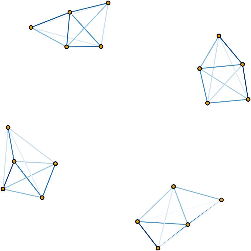
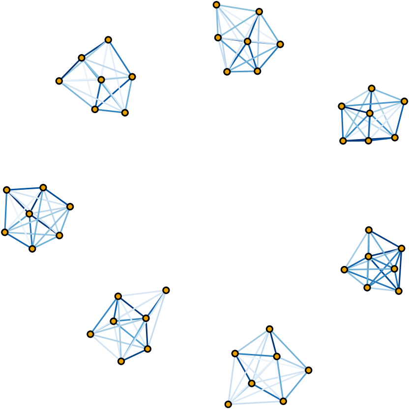
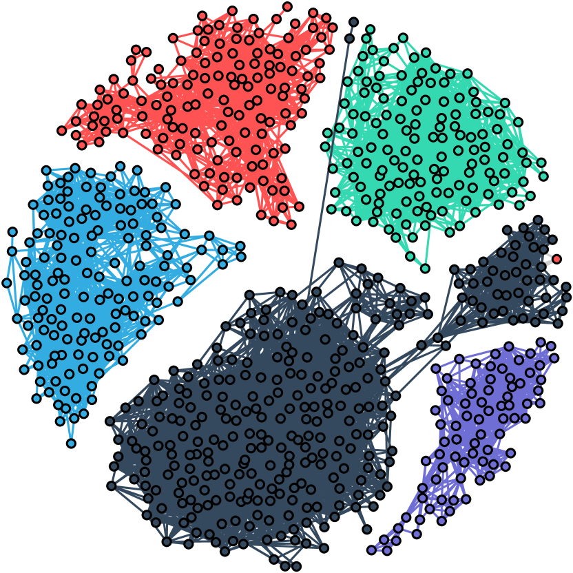
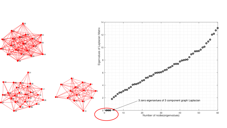
Figure 1 depicts a klimit-from𝑘k-component graph and its Laplacian eigenvalues with k𝑘k=3 connected components and zero eigenvalues.
Refer to caption
Figure 1: 333-component graph and its Laplacian matrix eigenvalues: three zero eigenvalues correspond to three components in the graph.

2.2.2 Connected sparse graph

A sparse graph is simply a graph with not many connections among the nodes. Often, making a graph highly sparse can split the graph into several disconnected components, which many times is undesirable (Sundin et al., 2017; Hassan-Moghaddam et al., 2016). The existing formulation cannot ensure both sparsity and connectedness, and there always exists a trade-off between the two properties. Within the formulation (17) we can achieve sparsity and connectedness by using the following spectral constraint:

𝒮λ={λ1=0,c1λ2λpc2}subscript𝒮𝜆formulae-sequencesubscript𝜆10subscript𝑐1subscript𝜆2subscript𝜆𝑝subscript𝑐2\displaystyle\mathcal{S}_{\lambda}=\{\lambda_{1}=0,c_{1}\leq\lambda_{2}\leq\ldots\leq\lambda_{p}\leq c_{2}\} (19)

with a proper choice of c1>0,c2>0formulae-sequencesubscript𝑐10subscript𝑐20c_{1}>0,c_{2}>0.

2.2.3 dlimit-from𝑑d-regular graph

All the nodes of a d𝑑d-regular graph have the same weighted degree (wi=d,i=1,2,,pformulae-sequencesubscript𝑤𝑖𝑑for-all𝑖12𝑝w_{i}=d,\;\forall i=1,2,\ldots,p), where weighted degree is defined as wi=j𝒩iwijsubscript𝑤𝑖subscript𝑗subscript𝒩𝑖subscript𝑤𝑖𝑗w_{i}=\sum_{j\in\mathcal{N}_{i}}w_{ij}, which implies:

Θ=dIΘA,diag(Θ)=d𝟏,ΘA𝟏=d𝟏.formulae-sequenceΘ𝑑𝐼subscriptΘ𝐴formulae-sequencediagΘ𝑑1subscriptΘ𝐴1𝑑1\displaystyle{{\Theta}}=d{{I}}-{{\Theta}}_{A},\;\;\text{diag}({{\Theta}})=d\mathbf{1},\;\;{{\Theta}}_{A}\mathbf{1}=d\mathbf{1}.

Within the above formulation (35) a dlimit-from𝑑d-regular structure on the matrix ΘΘ\Theta can be enforced by including the following constraints

𝒮λ={λ1=0,c1λ2λpc2},diag(Θ)=d𝟏.formulae-sequencesubscript𝒮𝜆formulae-sequencesubscript𝜆10subscript𝑐1subscript𝜆2subscript𝜆𝑝subscript𝑐2diagΘ𝑑1\displaystyle\mathcal{S}_{\lambda}=\{\lambda_{1}=0,c_{1}\leq\lambda_{2}\leq\cdots\leq\lambda_{p}\leq c_{2}\},\;\text{diag}({{\Theta}})=d\mathbf{1}. (20)

2.2.4 klimit-from𝑘k-component dlimit-from𝑑d-regular graph

A klimit-from𝑘k-component regular graph, also known as clustered regular graph is useful in providing improved perceptual grouping (Kim and Choi, 2009) for clustering applications. Within the above formulation (35) we can enforce this structure by including the following constraints

𝒮λ={{λj=0}j=1k,c1λk+1λpc2},diag(Θ)=d𝟏.formulae-sequencesubscript𝒮𝜆superscriptsubscriptsubscript𝜆𝑗0𝑗1𝑘subscript𝑐1subscript𝜆𝑘1subscript𝜆𝑝subscript𝑐2diagΘ𝑑1\displaystyle\mathcal{S}_{\lambda}=\{\{\lambda_{j}=0\}_{j=1}^{k},\ c_{1}\leq\lambda_{k+1}\leq\cdots\leq\lambda_{p}\leq c_{2}\},\;\text{diag}({{\Theta}})=d\mathbf{1}. (21)

2.2.5 Cospectral graphs

In many applications, it is motivated to learn ΘΘ\Theta with specific eigenvalues which is also known as cospectral graph learning (Godsil and McKay, 1982). One example is spectral sparsification of graphs (see Spielman and Teng, 2011; Loukas and Vandergheynst, 2018) which aims to learn a graph ΘΘ\Theta to approximate a given graph Θ¯¯Θ\bar{\Theta}, while ΘΘ\Theta is sparse and its eigenvalues λisubscript𝜆𝑖\lambda_{i} satisfy λi=f(λ¯i)subscript𝜆𝑖𝑓subscript¯𝜆𝑖\lambda_{i}=f(\bar{\lambda}_{i}), where {λi¯}i=1psuperscriptsubscript¯subscript𝜆𝑖𝑖1𝑝\{\bar{\lambda_{i}}\}_{i=1}^{p} are the eigenvalues of the given graph Θ¯¯Θ\bar{\Theta} and f𝑓f is some specific function. Therefore, for cospectral graph learning, we introduce the following constraint

𝒮λ={λi=f(λ¯i),i[1,p]}.subscript𝒮𝜆formulae-sequencesubscript𝜆𝑖𝑓subscript¯𝜆𝑖for-all𝑖1𝑝\displaystyle\mathcal{S}_{\lambda}=\{\lambda_{i}=f(\bar{\lambda}_{i}),\quad\forall i\in[1,p]\}. (22)

2.3 Structured Graph Learning Via Adjacency Spectral Constraints

To enforce spectral constraints on adjacency matrix ΘAsubscriptΘ𝐴{{\Theta}}_{A} (i.e., 𝒯(Θ)=ΘA𝒯ΘsubscriptΘ𝐴\mathcal{T}({{\Theta}})={{\Theta}}_{A} in (12)), we introduce the following optimization problem:

maximizeΘ,𝝍,Vloggdet(Θ)tr(ΘS)αh(Θ),subject toΘ𝒮Θ,ΘA=VDiag(𝝍)VT,𝝍𝒮ψ,VTV=I,Θ𝝍𝑉maximizegdetΘtrΘ𝑆𝛼Θsubject toformulae-sequenceΘsubscript𝒮Θformulae-sequencesubscriptΘ𝐴𝑉Diag𝝍superscript𝑉𝑇formulae-sequence𝝍subscript𝒮𝜓superscript𝑉𝑇𝑉𝐼\displaystyle\begin{array}[]{ll}\underset{{\Theta},{{\bm{{\psi}}}},{{V}}}{\text{maximize}}&\begin{array}[]{c}\hskip 21.33955pt\log\;\text{gdet}(\Theta)-\text{tr}\big{(}{\Theta S}\big{)}-\alpha h(\Theta),\end{array}\\ \text{subject to}&\begin{array}[t]{l}\hskip 21.33955pt\Theta\in\mathcal{S}_{\Theta},\ \Theta_{A}={V}{{{\text{Diag}}}(\bm{{\psi}})}{V}^{T},\ {\bm{{\psi}}}\in\mathcal{S}_{{\psi}},\ {V}^{T}{V}={I},\end{array}\end{array} (27)

where ΘΘ{{\Theta}} is the desired Laplacian matrix, ΘAsubscriptΘ𝐴{{\Theta}}_{A} is the corresponding adjacency matrix which admits the decomposition ΘA=VDiag(𝝍)VTsubscriptΘ𝐴𝑉Diag𝝍superscript𝑉𝑇{{\Theta}}_{A}={V}{{\text{Diag}}}({\bm{{\psi}}}){V}^{T} with 𝝍𝒮ψ𝝍subscript𝒮𝜓{\bm{{\psi}}}\in\mathcal{S}_{{\psi}} and VTV=Isuperscript𝑉𝑇𝑉𝐼{V}^{T}{V}={I}. We enforce ΘΘ{{\Theta}} to be a Laplacian matrix by the constraint Θ𝒮ΘΘsubscript𝒮Θ\Theta\in\mathcal{S}_{\Theta}, while we incorporate some specific spectral constraints on its adjacency matrix ΘAsubscriptΘ𝐴{{\Theta}}_{A} by forcing ΘA=VDiag(𝝍)VTsubscriptΘ𝐴𝑉Diag𝝍superscript𝑉𝑇{{\Theta}}_{A}={V}{{\text{Diag}}}({\bm{{\psi}}}){V}^{T}, with 𝒮ψsubscript𝒮𝜓\mathcal{S}_{{\psi}} containing priori spectral information of the desired graph structure.

Next, we will introduce various choices of 𝒮ψsubscript𝒮𝜓{\mathcal{S}}_{\psi} that will enable (27) to learn bipartite graph structures.

2.3.1 General bipartite graph

A graph is said to be bipartite if its vertex set can be partitioned into two disjoint subsets 𝒱=i=12𝒱i𝒱superscriptsubscript𝑖12subscript𝒱𝑖{\mathcal{V}}=\cup_{i=1}^{2}{\mathcal{V}}_{i} such that no two points belonging to the same subset are connected by an edge (Zha et al., 2001), i.e. for each (l,m)𝒱i×𝒱i𝑙𝑚subscript𝒱𝑖subscript𝒱𝑖(l,m)\in{\mathcal{V}}_{i}\times{\mathcal{V}}_{i} then (l,m)𝑙𝑚(l,m)\notin{\mathcal{E}}. Spectral graph theory states that a graph is bipartite if and only if the spectrum of the associated adjacency matrix is symmetric about the origin (Van Mieghem, 2010, Ch.5) (Mohar, 1997).

Theorem 2.

(see Mohar, 1997) A graph is bipartite if and only if the spectrum of the associated adjacency matrix is symmetric about the origin

𝒮ψ={ψi=ψpi+1,\displaystyle\mathcal{S}_{{\psi}}=\{\psi_{i}=-\psi_{p-i+1},\; i=1,,pfor-all𝑖1𝑝\displaystyle\forall i\;=1,\ldots,p (28)
ψ1ψ2ψp}.\displaystyle\psi_{1}\geq\psi_{2}\geq\cdots\geq\psi_{p}\big{\}}.

2.3.2 Connected bipartite graph

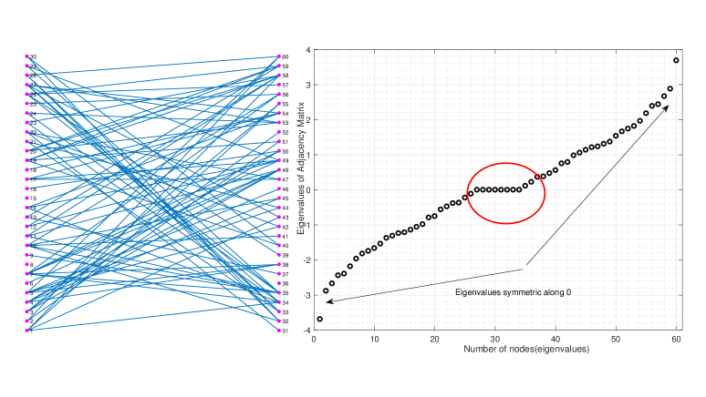
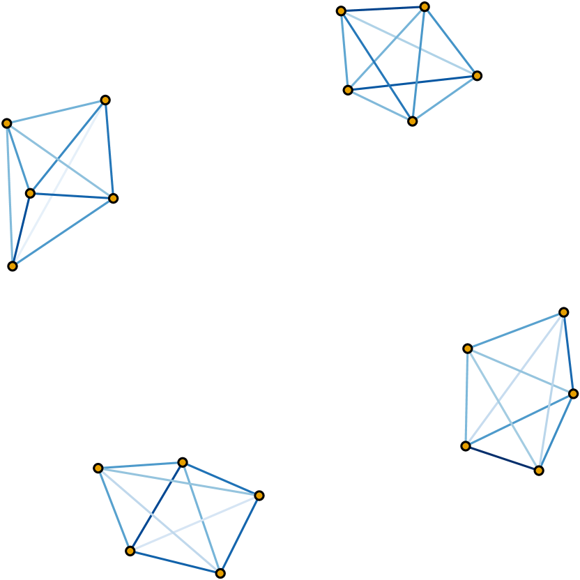
The Perron-Frobenius theorem states that if a graph is connected, then the largest eigenvalue ψpsubscript𝜓𝑝\psi_{p} of its adjacency matrix A𝐴{A} has multiplicity 1 (Mohar, 1997). Thus, a connected bipartite graph can be learned by including additional constraint on the multiplicity to be one on the largest and smallest eigenvalues, i.e. ψ1,ψpsubscript𝜓1subscript𝜓𝑝\psi_{1},\psi_{p} are not repeated. Figure 2 shows a connected bipartite graph and its adjacency symmetric eigenvalues.

Theorem 3.

(see Mohar, 1997) A graph is connected bipartite graph if and only if the spectrum of the associated adjacency matrix is symmetric about the origin with non-repeated extreme eigenvalues

𝒮ψ={ψi=ψpi+1,\displaystyle\mathcal{S}_{{\psi}}=\{\psi_{i}=-\psi_{p-i+1},\; i=1,,pfor-all𝑖1𝑝\displaystyle\forall\;i\;=1,\cdots,p (29)
ψ1>ψ2ψp1>ψp}.\displaystyle\psi_{1}>\psi_{2}\geq\cdots\geq\psi_{p-1}>\psi_{p}\big{\}}.
Refer to caption
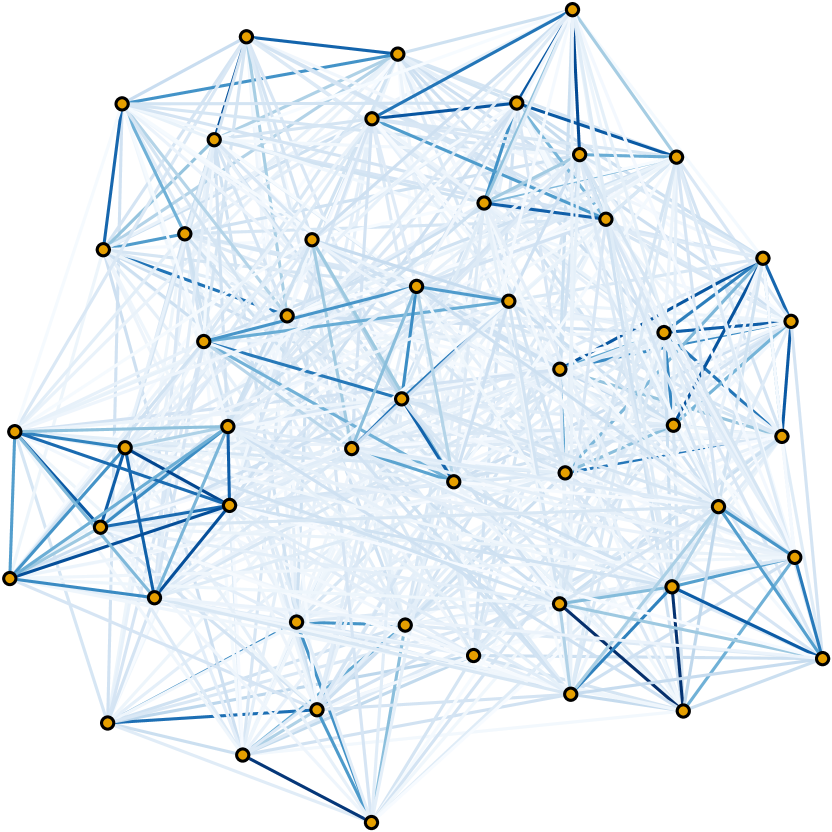
Figure 2: Bipartite graph adjacency matrix and its eigenvalues: eigenvalues are symmetric around 0.

2.4 Structured Graph Learning Via Joint Laplacian and Adjacency Spectral Constraints

To enforce spectral constraints on Laplacian matrix ΘΘ{{\Theta}} and adjacency matrix ΘAsubscriptΘ𝐴{{\Theta}}_{A}, we introduce the following optimization problem:

maximizeΘ,𝝀,𝝍,U,Vloggdet(Θ)tr(ΘS)αh(Θ),subject toΘ𝒮Θ,Θ=UDiag(𝝀)UT,ΘA=VDiag(𝝍)VT,𝝀𝒮λ,UTU=I,𝝍𝒮ψ,VTV=I.Θ𝝀𝝍𝑈𝑉maximizegdetΘtrΘ𝑆𝛼Θsubject toformulae-sequenceΘsubscript𝒮Θformulae-sequenceΘ𝑈Diag𝝀superscript𝑈𝑇subscriptΘ𝐴𝑉Diag𝝍superscript𝑉𝑇formulae-sequence𝝀subscript𝒮𝜆formulae-sequencesuperscript𝑈𝑇𝑈𝐼formulae-sequence𝝍subscript𝒮𝜓superscript𝑉𝑇𝑉𝐼\displaystyle\begin{array}[]{ll}\underset{{\Theta},{{\bm{\lambda}}},{\bm{{\psi}}},{{U}},{{V}}}{\text{maximize}}&\begin{array}[]{c}\hskip 21.33955pt\log\;\text{gdet}(\Theta)-\text{tr}\big{(}{\Theta S}\big{)}-\alpha h(\Theta),\end{array}\\ \text{subject to}&\begin{array}[t]{l}\hskip 21.33955pt\Theta\in\mathcal{S}_{\Theta},\ \Theta={U}{{{\text{Diag}}}({\bm{\lambda}})}{U}^{T},\ \Theta_{A}={V}{{\text{Diag}}}({\bm{{\psi}}}){V}^{T},\\ \hskip 21.33955pt{{\bm{\lambda}}}\in\mathcal{S}_{{\lambda}},\ {U}^{T}{U}={I},\ {\bm{{\psi}}}\in\mathcal{S}_{{\psi}},\ \ {V}^{T}{V}={I}.\end{array}\end{array} (35)

where ΘΘ{{\Theta}} is the desired Laplacian matrix which admits the decomposition Θ=UDiag(𝝀)UT,Θ𝑈Diag𝝀superscript𝑈𝑇\Theta={U}{{{\text{Diag}}}({\bm{\lambda}})}{U}^{T}, with 𝝀𝒮λ𝝀subscript𝒮𝜆{{\bm{\lambda}}}\in\mathcal{S}_{{\lambda}}, UTU=Isuperscript𝑈𝑇𝑈𝐼{U}^{T}{U}={I}, and ΘAsubscriptΘ𝐴{{\Theta}}_{A} is the corresponding adjacency matrix which admits the decomposition ΘA=VDiag(𝝍)VTsubscriptΘ𝐴𝑉Diag𝝍superscript𝑉𝑇{{\Theta}}_{A}={V}{{{\text{Diag}}}(\bm{{\psi}})}{V}^{T} with 𝝍𝒮ψ𝝍subscript𝒮𝜓{\bm{{\psi}}}\in\mathcal{S}_{{\psi}} and VTV=Isuperscript𝑉𝑇𝑉𝐼{V}^{T}{V}={I}. Observe that the above formulation learns a graph Laplacian matrix ΘΘ\Theta with a specific structure by enforcing the spectral constraints on the adjacency and Laplacian matrices simultaneously. Next, we will introduce various choices of 𝒮λsubscript𝒮𝜆{\mathcal{S}}_{\lambda} and 𝒮ψsubscript𝒮𝜓{\mathcal{S}}_{\psi} that will enable (35) to learn non-trivial complex graph popular graph structures.

2.4.1 klimit-from𝑘k-component bipartite graph

A klimit-from𝑘k-component bipartite graph, also known as bipartite graph clustering, has a significant relevance in many machine learning and financial applications (Zha et al., 2001). Recall that the bipartite structure can be enforced by utilizing the adjacency eigenvalues property (i.e., the constraints in (28)) and klimit-from𝑘k-component structure can be enforced by the Laplacian eigenvalues (i.e., the zero eigenvalues with multiplicity k𝑘k). These two disparate requirements can be simultaneously imposed in the current formulation (35), by choosing:

𝒮λ={{λj=0}j=1k,c1λk+1λpc2}subscript𝒮𝜆superscriptsubscriptsubscript𝜆𝑗0𝑗1𝑘subscript𝑐1subscript𝜆𝑘1subscript𝜆𝑝subscript𝑐2\displaystyle\mathcal{S}_{\lambda}=\{\{\lambda_{j}=0\}_{j=1}^{k},\ c_{1}\leq\lambda_{k+1}\leq\ldots\leq\lambda_{p}\leq c_{2}\} (36)
𝒮ψ={ψi:ψi=ψpi+1,i=1,,p}.subscript𝒮𝜓conditional-setsubscript𝜓𝑖formulae-sequencesubscript𝜓𝑖subscript𝜓𝑝𝑖1for-all𝑖1𝑝\displaystyle\mathcal{S}_{\psi}=\{\psi_{i}:\psi_{i}=-\psi_{p-i+1},\forall\;i=1,\cdots,p\}.

2.4.2 klimit-from𝑘k-component regular bipartite graph

The eigenvalue property of dlimit-from𝑑d-regular graph relates the eigenvalues of its adjacency matrix and Laplacian matrix, which is summarized in the following lemma.

Theorem 4.

(Mohar, 1997) Collecting the Laplacian eigenvalues in increasing order ({λj}j=1p\{\lambda_{j}\uparrow\}_{j=1}^{p}) and the adjacency eigenvalues in decreasing order ({ψi}i=1p\{\psi_{i}\downarrow\}_{i=1}^{p}), then the eigenvalue pairs for a d𝑑d-regular graph are related as follows:

λi=dψi,i=1,,p.formulae-sequencesubscript𝜆𝑖𝑑subscript𝜓𝑖for-all𝑖1𝑝\displaystyle\lambda_{i}=d-\psi_{i},\;\forall\;i=1,\cdots,p. (37)

A klimit-from𝑘k-component regular bipartite structure can be enforced by utilizing the adjacency eigenvalues property (for bipartite structure), Laplacian eigenvalues (for klimit-from𝑘k-component structure) along with the joint spectral properties for the regular graph structure:

𝒮λ={{λj=0}j=1k,c1λk+1λpc2}subscript𝒮𝜆superscriptsubscriptsubscript𝜆𝑗0𝑗1𝑘subscript𝑐1subscript𝜆𝑘1subscript𝜆𝑝subscript𝑐2\displaystyle\mathcal{S}_{\lambda}=\{\{\lambda_{j}=0\}_{j=1}^{k},\ c_{1}\leq\lambda_{k+1}\leq\ldots\leq\lambda_{p}\leq c_{2}\} (38)
𝒮ψ={ψi:ψi=dλi;ψi=ψpi+1,i=1,,p},subscript𝒮𝜓conditional-setsubscript𝜓𝑖formulae-sequencesubscript𝜓𝑖𝑑subscript𝜆𝑖formulae-sequencesubscript𝜓𝑖subscript𝜓𝑝𝑖1for-all𝑖1𝑝\displaystyle\mathcal{S}_{\psi}=\{\psi_{i}:\psi_{i}=d-\lambda_{i};\;\psi_{i}=-\psi_{p-i+1},\forall\;i=1,\cdots,p\},

2.5 Block Successive Upper-bound Minimization algorithm

The resulting optimization formulations presented in (17), (27), and (35) are still complicated. The aim here is to develop efficient optimization methods with low computational complexity based on the BSUM and majorization-minimization framework (Razaviyayn et al., 2013; Sun et al., 2016). To begin with, we present a general schematic of the BSUM optimization framework

minimize𝐱f(𝐱)subject to𝐱𝒳,𝐱minimize𝑓𝐱subject to𝐱𝒳\displaystyle\begin{array}[]{ll}\underset{{\mathbf{x}}}{\text{minimize}}&\begin{array}[]{c}f({\mathbf{x}})\end{array}\\ \text{subject to}&\begin{array}[t]{l}{\mathbf{x}}\in\mathcal{X},\end{array}\end{array} (43)

where the optimization variable 𝐱𝐱{\mathbf{x}} is partitioned into m𝑚m blocks as 𝐱=(𝐱1,𝐱2,,𝐱m)𝐱subscript𝐱1subscript𝐱2subscript𝐱𝑚{\mathbf{x}}=({\mathbf{x}}_{1},{\mathbf{x}}_{2},\cdots,{\mathbf{x}}_{m}), with 𝐱i𝒳isubscript𝐱𝑖subscript𝒳𝑖{\mathbf{x}}_{i}\in\mathcal{X}_{i}, 𝒳=i=1m𝒳i𝒳superscriptsubscriptproduct𝑖1𝑚subscript𝒳𝑖\mathcal{X}=\prod_{i=1}^{m}\mathcal{X}_{i} is a closed convex set, and f:𝐱:𝑓𝐱f:{\mathbf{x}}\rightarrow{\mathbb{R}} is a continuous function. At the tlimit-from𝑡t-th iteration, each block 𝐱isubscript𝐱𝑖{\mathbf{x}}_{i} is updated in a cyclic order by solving the following:

minimize𝐱igi(𝐱i|𝐱1t,,𝐱i1t,𝐱i+1t1,,𝐱mt1),subject to𝐱i𝒳i,subscript𝐱𝑖minimizesubscript𝑔𝑖conditionalsubscript𝐱𝑖superscriptsubscript𝐱1𝑡superscriptsubscript𝐱𝑖1𝑡superscriptsubscript𝐱𝑖1𝑡1superscriptsubscript𝐱𝑚𝑡1subject tosubscript𝐱𝑖subscript𝒳𝑖\displaystyle\begin{array}[]{ll}\underset{{\mathbf{x}}_{i}}{\text{minimize}}&\begin{array}[]{c}g_{i}({\mathbf{x}}_{i}|{\mathbf{x}}_{1}^{t},\cdots,{\mathbf{x}}_{i-1}^{t},{\mathbf{x}}_{i+1}^{t-1},\cdots,{\mathbf{x}}_{m}^{t-1}),\end{array}\\ \text{subject to}&\begin{array}[t]{l}{\mathbf{x}}_{i}\in\mathcal{X}_{i},\end{array}\end{array} (48)

where gi(𝐱i|𝐲it)subscript𝑔𝑖conditionalsubscript𝐱𝑖superscriptsubscript𝐲𝑖𝑡g_{i}({\mathbf{x}}_{i}|{\mathbf{y}}_{i}^{t}) with 𝐲it:=(𝐱1t,,𝐱i1t,𝐱it1,𝐱i+1t1,,𝐱mt1)assignsuperscriptsubscript𝐲𝑖𝑡superscriptsubscript𝐱1𝑡superscriptsubscript𝐱𝑖1𝑡superscriptsubscript𝐱𝑖𝑡1superscriptsubscript𝐱𝑖1𝑡1superscriptsubscript𝐱𝑚𝑡1{\mathbf{y}}_{i}^{t}:=({\mathbf{x}}_{1}^{t},\cdots,{\mathbf{x}}_{i-1}^{t},{\mathbf{x}}_{i}^{t-1},{\mathbf{x}}_{i+1}^{t-1},\cdots,{\mathbf{x}}_{m}^{t-1}) is a majorization function of f(𝐱)𝑓𝐱f({\mathbf{x}}) at 𝐲itsuperscriptsubscript𝐲𝑖𝑡{\mathbf{y}}_{i}^{t} satisfying

gi(𝐱i|𝐲it)is continuous in (𝐱i,𝐲it),i,subscript𝑔𝑖conditionalsubscript𝐱𝑖superscriptsubscript𝐲𝑖𝑡is continuous in subscript𝐱𝑖superscriptsubscript𝐲𝑖𝑡for-all𝑖\displaystyle g_{i}({\mathbf{x}}_{i}|{\mathbf{y}}_{i}^{t})\;\text{is continuous in }\;({\mathbf{x}}_{i},{\mathbf{y}}_{i}^{t}),\;\forall\;i, (49a)
gi(𝐱it|𝐲it)=f(𝐱1t,,𝐱i1t,𝐱it,𝐱i+1t1,,𝐱mt1),subscript𝑔𝑖conditionalsubscriptsuperscript𝐱𝑡𝑖superscriptsubscript𝐲𝑖𝑡𝑓superscriptsubscript𝐱1𝑡superscriptsubscript𝐱𝑖1𝑡superscriptsubscript𝐱𝑖𝑡superscriptsubscript𝐱𝑖1𝑡1superscriptsubscript𝐱𝑚𝑡1\displaystyle g_{i}({\mathbf{x}}^{t}_{i}|{\mathbf{y}}_{i}^{t})=f({\mathbf{x}}_{1}^{t},\cdots,{\mathbf{x}}_{i-1}^{t},{\mathbf{x}}_{i}^{t},{\mathbf{x}}_{i+1}^{t-1},\cdots,{\mathbf{x}}_{m}^{t-1}), (49b)
gi(𝐱i|𝐲it)f(𝐱1t,,𝐱i1t,𝐱i,𝐱i+1t1,,𝐱mt1),𝐱i𝒳i,𝐲i𝒳,i,formulae-sequencesubscript𝑔𝑖conditionalsubscript𝐱𝑖superscriptsubscript𝐲𝑖𝑡𝑓superscriptsubscript𝐱1𝑡superscriptsubscript𝐱𝑖1𝑡subscript𝐱𝑖superscriptsubscript𝐱𝑖1𝑡1superscriptsubscript𝐱𝑚𝑡1formulae-sequencefor-allsubscript𝐱𝑖subscript𝒳𝑖for-allsubscript𝐲𝑖𝒳for-all𝑖\displaystyle g_{i}({\mathbf{x}}_{i}|{\mathbf{y}}_{i}^{t})\geq f({\mathbf{x}}_{1}^{t},\cdots,{\mathbf{x}}_{i-1}^{t},{\mathbf{x}}_{i},{\mathbf{x}}_{i+1}^{t-1},\cdots,{\mathbf{x}}_{m}^{t-1}),\;\forall\;{\mathbf{x}}_{i}\in{\mathcal{X}}_{i},\forall\;{\mathbf{y}}_{i}\in{\mathcal{X}},\forall\;i, (49c)
gi(𝐱i;𝐝i|𝐲it)|𝐱i=𝐱it=f(𝐱1t,,𝐱i1t,𝐱i,𝐱i+1t1,,𝐱mt1;𝐝),evaluated-atsubscriptsuperscript𝑔𝑖subscript𝐱𝑖conditionalsubscript𝐝𝑖superscriptsubscript𝐲𝑖𝑡subscript𝐱𝑖superscriptsubscript𝐱𝑖𝑡superscript𝑓superscriptsubscript𝐱1𝑡superscriptsubscript𝐱𝑖1𝑡subscript𝐱𝑖superscriptsubscript𝐱𝑖1𝑡1superscriptsubscript𝐱𝑚𝑡1𝐝\displaystyle{g^{\prime}_{i}({\mathbf{x}}_{i};\mathbf{d}_{i}|{\mathbf{y}}_{i}^{t})|_{{\mathbf{x}}_{i}={\mathbf{x}}_{i}^{t}}=f^{\prime}({\mathbf{x}}_{1}^{t},\cdots,{\mathbf{x}}_{i-1}^{t},{\mathbf{x}}_{i},{\mathbf{x}}_{i+1}^{t-1},\cdots,{\mathbf{x}}_{m}^{t-1};\mathbf{d})},
𝐝=(𝟎,,𝐝i,,𝟎)such that𝐱it+𝐝i𝒳i,i,formulae-sequencefor-all𝐝0subscript𝐝𝑖0such thatsuperscriptsubscript𝐱𝑖𝑡subscript𝐝𝑖subscript𝒳𝑖for-all𝑖\displaystyle\hskip 85.35826pt{\forall\;\;\mathbf{d}=(\mathbf{0},\cdots,\mathbf{d}_{i},\cdots,\mathbf{0})\;\text{such that}\;{\mathbf{x}}_{i}^{t}+\mathbf{d}_{i}\in{\mathcal{X}}_{i},\;\forall\;i,} (49d)

where f(𝐱;𝐝)superscript𝑓𝐱𝐝f^{\prime}({\mathbf{x}};\mathbf{d}) stands for the directional derivative at 𝐱𝐱{\mathbf{x}} along 𝐝𝐝\mathbf{d} (Razaviyayn et al., 2013). In summary, the framework is based on a sequential inexact block coordinate approach, which updates the variable in one block keeping the other blocks fixed. If the surrogate functions gisubscript𝑔𝑖g_{i} is properly chosen, then the solution to (48) could be easier to obtain than solving (43) directly.

3 Structured Graph Learning Via Laplacian Spectral Constraints (SGL)

In this section, we develop a BSUM-based algorithm for Structured Graph learning via Laplacian spectral constraints (SGL). In particular, we consider solving (17) under klimit-from𝑘k-component Laplacian spectral constraints (18). To enforce sparsity we use the 1limit-fromsubscript1\ell_{1}-regularization function (i.e., h(Θ):=Θ1assignΘsubscriptnormΘ1h(\Theta):=\left\|{{\Theta}}\right\|_{1}). Next observing that the sign of ΘΘ{{\Theta}} is fixed by the constraints Θij0forijsubscriptΘ𝑖𝑗0for𝑖𝑗{{\Theta}}_{ij}\leq 0\,{\rm for}\,i\neq j and Θij0fori=jsubscriptΘ𝑖𝑗0for𝑖𝑗{{\Theta}}_{ij}\geq 0\,{\rm for}\,i=j, the regularization term αΘ1𝛼subscriptnormΘ1\alpha\left\|{{\Theta}}\right\|_{1} can be written by tr(ΘH)trΘ𝐻\text{tr}\left({{\Theta}}{{H}}\right), where H=α(2I𝟏𝟏T)𝐻𝛼2𝐼superscript11𝑇{{H}}=\alpha(2{{I}}-{\mathbf{1}}{\mathbf{1}}^{T}), problem (17) becomes

minimizeΘ,𝝀,Uloggdet(Θ)+tr(ΘK),subject toΘ𝒮Θ,Θ=UDiag(𝝀)UT,𝝀𝒮λ,UTU=I,Θ𝝀𝑈minimizegdetΘtrΘ𝐾subject toformulae-sequenceΘsubscript𝒮Θformulae-sequenceΘ𝑈Diag𝝀superscript𝑈𝑇formulae-sequence𝝀subscript𝒮𝜆superscript𝑈𝑇𝑈𝐼\displaystyle\begin{array}[]{ll}\underset{{{{\Theta}}},{{\bm{\lambda}}},{{U}}}{\text{minimize}}&\begin{array}[]{c}-\log\;\text{gdet}({{\Theta}})+\text{tr}\left({{\Theta}}{{K}}\right),\end{array}\\ \text{subject to}&\begin{array}[t]{l}{{{\Theta}}}\in{\mathcal{S}}_{{{\Theta}}},\ {{\Theta}}={{U}}{{\text{Diag}}}({\bm{\lambda}}){{U}}^{T},\ {\bm{\lambda}}\in{\mathcal{S}}_{\lambda},\ {{U}}^{T}{{U}}={{I}},\end{array}\end{array} (54)

where K=S+H𝐾𝑆𝐻{{K}}=S+{{H}}. The resulting problem is complicated and intractable in the current form due to i) Laplacian structural constraints 𝒮Θsubscript𝒮Θ{\mathcal{S}}_{{{\Theta}}}, ii) coupling variables Θ=UDiag(𝝀)UTΘ𝑈Diag𝝀superscript𝑈𝑇{{\Theta}}={{U}}{{\text{Diag}}}({\bm{\lambda}}){{U}}^{T}, and iii) generalized determinant on ΘΘ{{\Theta}}. In order to derive a more feasible formulation, we first introduce a linear operator {\mathcal{L}} which transforms the Laplacian structural constraints to simple algebraic constraints and then relax the eigen-decomposition expression into the objective function.

3.1 Graph Laplacian operator {\mathcal{L}}

The Laplacian matrix ΘΘ{{\Theta}} belonging to 𝒮Θsubscript𝒮Θ{\mathcal{S}}_{{{\Theta}}} satisfies i) Θij=Θji0subscriptΘ𝑖𝑗subscriptΘ𝑗𝑖0\Theta_{ij}=\Theta_{ji}\leq 0, ii) Θ𝟏=𝟎Θ10{{\Theta}}{\mathbf{1}}={\mathbf{0}}, implying the target matrix is symmetric with degrees of freedom of ΘΘ{{{\Theta}}} equal to p(p1)/2𝑝𝑝12p(p-1)/2. Therefore, we introduce a linear operator {\mathcal{L}} that transforms a non-negative vector 𝐰+p(p1)/2𝐰superscriptsubscript𝑝𝑝12\mathbf{{w}}\in\mathbb{R}_{+}^{p(p-1)/2} into the matrix 𝐰p×p𝐰superscript𝑝𝑝{\mathcal{L}}\mathbf{{w}}\in{\mathbb{R}}^{p\times p} that satisfies the Laplacian constraints ([𝐰]ij=[𝐰]ji,forijformulae-sequencesubscriptdelimited-[]𝐰𝑖𝑗subscriptdelimited-[]𝐰𝑗𝑖for𝑖𝑗[{\mathcal{L}}\mathbf{{w}}]_{ij}=[{\mathcal{L}}\mathbf{{w}}]_{ji},{\rm for}\,i\neq j and [𝐰]𝟏=𝟎delimited-[]𝐰10[{\mathcal{L}}\mathbf{{w}}]{\mathbf{1}}={\mathbf{0}}).

Definition 2.

The linear operator :𝐰+p(p1)2𝐰p×p:𝐰superscriptsubscript𝑝𝑝12𝐰superscript𝑝𝑝{\mathcal{L}}:\mathbf{{w}}\in\mathbb{R}_{+}^{\frac{p(p-1)}{2}}\rightarrow{\mathcal{L}}\mathbf{{w}}\in{\mathbb{R}}^{p\times p} is defined as

[𝐰]ij={wi+dji>j,[𝐰]jii<j,ij[𝐰]iji=j,subscriptdelimited-[]𝐰𝑖𝑗casessubscript𝑤𝑖subscript𝑑𝑗𝑖𝑗subscriptdelimited-[]𝐰𝑗𝑖𝑖𝑗subscript𝑖𝑗subscriptdelimited-[]𝐰𝑖𝑗𝑖𝑗[{\mathcal{L}}\mathbf{{w}}]_{ij}=\begin{cases}-w_{i+d_{j}}\;&\;\;i>j,\\ [{\mathcal{L}}\mathbf{{w}}]_{ji}\;&\;\;i<j,\\ \sum_{i\neq j}[{\mathcal{L}}\mathbf{{w}}]_{ij}\;&\;\;i=j,\end{cases}

where dj=j+j12(2pj).subscript𝑑𝑗𝑗𝑗122𝑝𝑗d_{j}=-j+\frac{j-1}{2}(2p-j).

We derive the adjoint operator superscript{\mathcal{L}}^{*} of {\mathcal{L}} by making superscript{\mathcal{L}}^{*} satisfy 𝐰,Y=𝐰,Y𝐰𝑌𝐰superscript𝑌\langle{\mathcal{L}}\mathbf{{w}},{{Y}}\rangle=\langle\mathbf{{w}},{\mathcal{L}}^{*}{{Y}}\rangle.

Lemma 1.

The adjoint operator :Yp×pYp(p1)2:superscript𝑌superscript𝑝𝑝maps-tosuperscript𝑌superscript𝑝𝑝12{\mathcal{L}}^{*}:{{Y}}\in{\mathbb{R}}^{p\times p}\mapsto{\mathcal{L}}^{*}{{Y}}\in{\mathbb{R}}^{\frac{p(p-1)}{2}} is defined by

[Y]k=yi,iyi,jyj,i+yj,j,k=ij+j12(2pj),formulae-sequencesubscriptdelimited-[]superscript𝑌𝑘subscript𝑦𝑖𝑖subscript𝑦𝑖𝑗subscript𝑦𝑗𝑖subscript𝑦𝑗𝑗𝑘𝑖𝑗𝑗122𝑝𝑗[{\mathcal{L}}^{*}{{Y}}]_{k}=y_{i,i}-y_{i,j}-y_{j,i}+y_{j,j},\;\;k=i-j+\frac{j-1}{2}(2p-j),

where i,j+𝑖𝑗superscripti,j\in\mathbb{Z}^{+} satisfy k=ij+j12(2pj)𝑘𝑖𝑗𝑗122𝑝𝑗k=i-j+\frac{j-1}{2}(2p-j) and i>j𝑖𝑗i>j.

A toy example is given to illustrate the operators {\mathcal{L}} and superscript{\mathcal{L}}^{*} more clearly. Consider a weight vector 𝐰=[w1,w2,w3,w4,w5,w6]T𝐰superscriptsubscript𝑤1subscript𝑤2subscript𝑤3subscript𝑤4subscript𝑤5subscript𝑤6𝑇\mathbf{{w}}=[w_{1},w_{2},w_{3},w_{4},w_{5},w_{6}]^{T}. The Laplacian operator {\mathcal{L}} on 𝐰𝐰\mathbf{{w}} gives

𝐰=[i=1,2,3wiw1w2w3w1i=1,4,5wiw4w5w2w4i=2,4,6wiw6w3w5w6i=3,5,6wi].𝐰delimited-[]subscript𝑖123subscript𝑤𝑖subscript𝑤1subscript𝑤2subscript𝑤3subscript𝑤1subscript𝑖145subscript𝑤𝑖subscript𝑤4subscript𝑤5subscript𝑤2subscript𝑤4subscript𝑖246subscript𝑤𝑖subscript𝑤6subscript𝑤3subscript𝑤5subscript𝑤6subscript𝑖356subscript𝑤𝑖{\mathcal{L}}\mathbf{{w}}=\left[\begin{array}[]{cccc}\sum_{i=1,2,3}w_{i}&-w_{1}&-w_{2}&-w_{3}\\ -w_{1}&\sum_{i=1,4,5}w_{i}&-w_{4}&-w_{5}\\ -w_{2}&-w_{4}&\sum_{i=2,4,6}w_{i}&-w_{6}\\ -w_{3}&-w_{5}&-w_{6}&\sum_{i=3,5,6}w_{i}\par\end{array}\right]. (55)

The operation of superscript{\mathcal{L}}^{*} on a 4×4444\times 4 symmetric matrix Y𝑌{{Y}} returns a vector

Y=[y11y21y12+y22y11y31y13+y33y11y41y14+y44y22y32y23+y33y22y42y24+y44y33y43y34+y44].superscript𝑌delimited-[]subscript𝑦11subscript𝑦21subscript𝑦12subscript𝑦22subscript𝑦11subscript𝑦31subscript𝑦13subscript𝑦33subscript𝑦11subscript𝑦41subscript𝑦14subscript𝑦44subscript𝑦22subscript𝑦32subscript𝑦23subscript𝑦33subscript𝑦22subscript𝑦42subscript𝑦24subscript𝑦44subscript𝑦33subscript𝑦43subscript𝑦34subscript𝑦44{\mathcal{L}}^{*}{{Y}}=\left[\begin{array}[]{c}y_{11}-y_{21}-y_{12}+y_{22}\\ y_{11}-y_{31}-y_{13}+y_{33}\\ y_{11}-y_{41}-y_{14}+y_{44}\\ y_{22}-y_{32}-y_{23}+y_{33}\\ y_{22}-y_{42}-y_{24}+y_{44}\\ y_{33}-y_{43}-y_{34}+y_{44}\end{array}\right]. (56)

By the definition of {\mathcal{L}}, we have Lemma 2.

Lemma 2.

The operator norm 2subscriptnorm2\|{\mathcal{L}}\|_{2} is 2p2𝑝\sqrt{2p}, where 2sup𝐱=1𝐱Fapproaches-limitsubscriptnorm2subscriptsupremumnorm𝐱1subscriptnorm𝐱𝐹\|{\mathcal{L}}\|_{2}\doteq\sup_{\left\|{\mathbf{x}}\right\|=1}\left\|{\mathcal{L}}{\mathbf{x}}\right\|_{F} with 𝐱p(p1)2𝐱superscript𝑝𝑝12{\mathbf{x}}\in{\mathbb{R}}^{\frac{p(p-1)}{2}}.

Proof.

Follows from the definitions of {\mathcal{L}} and superscript{\mathcal{L}}^{*}: see Appendix 8.1 for detailed proof. ∎

We have introduced the operator {\mathcal{L}} that helps to transform the complicated structural matrix variable ΘΘ{{\Theta}} to a simple vector variable 𝐰𝐰\mathbf{{w}}. The linear operator {\mathcal{L}} is an important component of the SGL framework.

3.2 SGL algorithm

To solve (54), we represent the Laplacian matrix Θ𝒮ΘΘsubscript𝒮Θ{{\Theta}}\in{\mathcal{S}}_{{{\Theta}}} as 𝐰𝐰{\mathcal{L}}\mathbf{{w}} and then develop an algorithm based on quadratic methods (Nikolova and Ng, 2005; Ying et al., 2018). We introduce the term β2𝐰UDiag(𝝀)UTF2𝛽2superscriptsubscriptnorm𝐰𝑈Diag𝝀superscript𝑈𝑇𝐹2\frac{\beta}{2}\|{\mathcal{L}}\mathbf{{w}}-{{{U}}}{{\text{Diag}}}({\bm{\lambda}}){{{U}}}^{T}\|_{F}^{2} to keep 𝐰𝐰{\mathcal{L}}\mathbf{{w}} close to UDiag(𝝀)UT𝑈Diag𝝀superscript𝑈𝑇{{{U}}}{{\text{Diag}}}({\bm{\lambda}}){{{U}}}^{T} instead of exactly solving the constraint 𝐰=UDiag(𝝀)UT𝐰𝑈Diag𝝀superscript𝑈𝑇{\mathcal{L}}\mathbf{{w}}={{{U}}}{{\text{Diag}}}({\bm{\lambda}}){{{U}}}^{T}, where β>0𝛽0\beta>0. Note that this relaxation can be made tight by choosing β𝛽\beta sufficient large or iteratively increasing β𝛽\beta. Now, the original problem can be formulated as

minimize𝐰,𝝀,Uloggdet(Diag(𝝀))+tr(K𝐰)+β2𝐰UDiag(𝝀)UTF2,subject to𝐰0,𝝀𝒮λ,UTU=I,𝐰𝝀𝑈minimizegdetDiag𝝀tr𝐾𝐰𝛽2superscriptsubscriptnorm𝐰𝑈Diag𝝀superscript𝑈𝑇𝐹2subject toformulae-sequence𝐰0formulae-sequence𝝀subscript𝒮𝜆superscript𝑈𝑇𝑈𝐼\displaystyle\begin{array}[]{ll}\underset{{\mathbf{{w}}},{{\bm{\lambda}}},{{{U}}}}{\text{minimize}}&\begin{array}[]{c}-\log\text{gdet}({{\text{Diag}}}({\bm{\lambda}}))+\text{tr}\left({{K}}{\mathcal{L}}\mathbf{{w}}\right)+\frac{\beta}{2}\|{\mathcal{L}}\mathbf{{w}}-{{U}}{{\text{Diag}}}({\bm{\lambda}}){{U}}^{T}\|_{F}^{2},\end{array}\\ \text{subject to}&\begin{array}[t]{l}\mathbf{{w}}\geq 0,\ {\bm{\lambda}}\in{\mathcal{S}}_{\lambda},\ {{U}}^{T}{{U}}={{I}},\end{array}\end{array} (61)

where 𝐰0𝐰0\mathbf{{w}}\geq 0 means each entry of 𝐰𝐰\mathbf{{w}} is non-negative. When solving (61) to learn the klimit-from𝑘k-component graph structure with the constraints in (18), the first k𝑘k zero eigenvalues as well as the corresponding eigenvectors can be dropped from the optimization formulation. Now the 𝝀𝝀{\bm{\lambda}} only contains q=pk𝑞𝑝𝑘q=p-k non-zero eigenvalues in increasing order {λj}j=k+1psuperscriptsubscriptsubscript𝜆𝑗𝑗𝑘1𝑝\{\lambda_{j}\}_{j=k+1}^{p}, then we can replace generalized determinant with determinant on Diag(𝝀)Diag𝝀{{\text{Diag}}}({\bm{\lambda}}) in (61). Up×q𝑈superscript𝑝𝑞{{{U}}}\in\mathbb{R}^{p\times q} contains the eigenvectors corresponding to the non-zero eigenvalues in the same order, and the orthogonality constraints on U𝑈{{U}} becomes UTU=Iqsuperscript𝑈𝑇𝑈subscript𝐼𝑞{{U}}^{T}{{U}}={{I}}_{q}. The non-zero eigenvalues are ordered and lie in the given set,

𝒮λ={c1λk+1λpc2}.subscript𝒮𝜆subscript𝑐1subscript𝜆𝑘1subscript𝜆𝑝subscript𝑐2\displaystyle\mathcal{S}_{{\lambda}}=\{\ c_{1}\leq\lambda_{k+1}\leq\ldots\leq\lambda_{p}\leq c_{2}\}. (62)

Collecting the variables in three block as 𝐱=(𝐰p(p1)/2,𝝀q,Up×q)𝐱formulae-sequence𝐰superscript𝑝𝑝12formulae-sequence𝝀superscript𝑞𝑈superscript𝑝𝑞{\mathbf{x}}=\left(\mathbf{{w}}\in{\mathbb{R}}^{p(p-1)/2},{\bm{\lambda}}\in{\mathbb{R}}^{q},{{U}}\in{\mathbb{R}}^{p\times q}\right), we develop a BSUM-based algorithm which updates only one variable each time with the other variables fixed.

3.2.1 Update of 𝐰𝐰\mathbf{{w}}

Treating 𝐰𝐰\mathbf{{w}} as a variable with U𝑈{{U}} and 𝝀𝝀{\bm{\lambda}} fixed, and ignoring the terms independent of 𝐰𝐰\mathbf{{w}}, we have the following sub-problem:

minimize𝐰0tr(K𝐰)+β2𝐰UDiag(𝝀)UTF2.𝐰0minimizetr𝐾𝐰𝛽2superscriptsubscriptnorm𝐰𝑈Diag𝝀superscript𝑈𝑇𝐹2\displaystyle\underset{\mathbf{{w}}\geq 0}{\text{minimize}}\qquad\text{tr}\left({{K}}{\mathcal{L}}\mathbf{{w}}\right)+\frac{\beta}{2}\|{\mathcal{L}}\mathbf{{w}}-{{U}}{{\text{Diag}}}({\bm{\lambda}}){{{U}}}^{T}\|_{F}^{2}. (63)

The problem (63) can be written as a non-negative quadratic problem,

minimize𝐰0f(𝐰)=12𝐰F2𝐜T𝐰,𝐰0minimize𝑓𝐰12subscriptsuperscriptnorm𝐰2𝐹superscript𝐜𝑇𝐰\displaystyle\underset{\mathbf{{w}}\geq 0}{\text{minimize}}\qquad f(\mathbf{{w}})=\frac{1}{2}\left\|{\mathcal{L}}\mathbf{{w}}\right\|^{2}_{F}-{{\mathbf{c}}}^{T}\mathbf{{w}}, (64)

where 𝐜=(UDiag(𝝀)UTβ1K)𝐜superscript𝑈Diag𝝀superscript𝑈𝑇superscript𝛽1𝐾{\mathbf{c}}={\mathcal{L}}^{*}({{U}}{{\text{Diag}}}({\bm{\lambda}}){{{U}}}^{T}-\beta^{-1}{{K}}).

Lemma 3.

The sub-problem (64) is a strictly convex optimization problem.

Proof.

From the definition of operator {\mathcal{L}} and the property of its adjoint superscript{\mathcal{L}}^{*}, we have

𝐰F2=𝐰,𝐰=𝐰,𝐰=𝐰T𝐰>0,𝐰𝟎.formulae-sequencesuperscriptsubscriptnorm𝐰𝐹2𝐰𝐰𝐰superscript𝐰superscript𝐰𝑇superscript𝐰0for-all𝐰0\displaystyle\|{\mathcal{L}}\mathbf{{w}}\|_{F}^{2}=\langle{\mathcal{L}}\mathbf{{w}},{\mathcal{L}}\mathbf{{w}}\rangle=\langle\mathbf{{w}},{\mathcal{L}}^{*}{\mathcal{L}}\mathbf{{w}}\rangle=\mathbf{{w}}^{T}{\mathcal{L}}^{*}{\mathcal{L}}\mathbf{{w}}>0,\;\;\forall\;\mathbf{{w}}\neq{\mathbf{0}}. (65)

The above result implies that f(𝐰)𝑓𝐰f(\mathbf{{w}}) is a strictly convex function. Together with the fact that the non-negativity set is convex, we conclude the sub-problem (64) is strictly convex. But, it is not possible here to derive a closed-form solution due to the non-negativity constraint (𝐰0𝐰0\mathbf{{w}}\geq 0), and thus we derive a majorijation function. ∎

Lemma 4.

The function f(𝐰)𝑓𝐰f(\mathbf{{w}}) in (64) is majorized at 𝐰tsuperscript𝐰𝑡\mathbf{{w}}^{t} by the function

g(𝐰|𝐰t)𝑔conditional𝐰superscript𝐰𝑡\displaystyle g(\mathbf{{w}}|\mathbf{{w}}^{t}) =f(𝐰t)+(𝐰𝐰t)Tf(𝐰t)+L12𝐰𝐰t2,absent𝑓superscript𝐰𝑡superscript𝐰superscript𝐰𝑡𝑇𝑓superscript𝐰𝑡subscript𝐿12superscriptnorm𝐰superscript𝐰𝑡2\displaystyle=f(\mathbf{{w}}^{t})+(\mathbf{{w}}-\mathbf{{w}}^{t})^{T}\nabla f(\mathbf{{w}}^{t})+\frac{L_{1}}{2}\left\|\mathbf{{w}}-\mathbf{{w}}^{t}\right\|^{2}, (66)

where 𝐰tsuperscript𝐰𝑡\mathbf{{w}}^{t} is the update from previous iteration and L1=22=2psubscript𝐿1superscriptsubscriptnorm222𝑝L_{1}=\left\|{\mathcal{L}}\right\|_{2}^{2}=2p (see Lemma 2).

It is easy to check the conditions (49) for the majorization function (See more details in Sun et al., 2016; Song et al., 2015) and we ignore the proof here. Note that the majorization function as g(𝐰|𝐰t)𝑔conditional𝐰superscript𝐰𝑡g(\mathbf{{w}}|\mathbf{{w}}^{t}) in (66) is in accordance with the requirement of the majorization as in (49b), because in the problem (64), 𝐰tsuperscript𝐰𝑡\mathbf{{w}}^{t} and the other coordinates (𝝀t,Utsuperscript𝝀𝑡superscript𝑈𝑡{\bm{\lambda}}^{t},U^{t}) are fixed. For notational brevity, we present the majorization function as g(𝐰|𝐰t)𝑔conditional𝐰superscript𝐰𝑡g(\mathbf{{w}}|\mathbf{{w}}^{t}) instead of g(𝐰|𝐰t,Ut,𝝀t)𝑔conditional𝐰superscript𝐰𝑡superscript𝑈𝑡superscript𝝀𝑡g(\mathbf{{w}}|\mathbf{{w}}^{t},U^{t},{\bm{\lambda}}^{t}).

After ignoring the constant terms in (66), the majorized problem of (64) at 𝐰tsuperscript𝐰𝑡\mathbf{{w}}^{t} is given by

minimize𝐰0g(𝐰|𝐰t)=12𝐰T𝐰𝒂T𝐰,𝐰0minimize𝑔conditional𝐰superscript𝐰𝑡12superscript𝐰𝑇𝐰superscript𝒂𝑇𝐰\displaystyle\underset{\mathbf{{w}}\geq 0}{\text{minimize}}\qquad g(\mathbf{{w}}|\mathbf{{w}}^{t})=\frac{1}{2}{\mathbf{{w}}}^{T}\mathbf{{w}}-{\bm{a}}^{T}\mathbf{{w}}, (67)

where a=𝐰t1L1f(𝐰t)𝑎superscript𝐰𝑡1subscript𝐿1𝑓superscript𝐰𝑡{a}=\mathbf{{w}}^{t}-\frac{1}{L_{1}}\nabla f(\mathbf{{w}}^{t}) and f(𝐰t)=(𝐰t)𝐜𝑓superscript𝐰𝑡superscriptsuperscript𝐰𝑡𝐜\nabla f(\mathbf{{w}}^{t})={\mathcal{L}}^{*}({\mathcal{L}}\mathbf{{w}}^{t})-\mathbf{c}.

Lemma 5.

From the KKT optimality conditions we can easily obtain the optimal solution to (67) as

𝐰t+1=(𝐰t1L1f(𝐰t))+,superscript𝐰𝑡1superscriptsuperscript𝐰𝑡1subscript𝐿1𝑓superscript𝐰𝑡\displaystyle\mathbf{{w}}^{t+1}=\left(\mathbf{{w}}^{t}-\frac{1}{L_{1}}\nabla f(\mathbf{{w}}^{t})\right)^{+}, (68)

where (x)+:=max(x,0)assignsuperscript𝑥𝑥0(x)^{+}:=\max(x,0).

3.2.2 Update of U𝑈{{U}}

Treating U𝑈{{U}} as a variable block, and fixing for 𝐰𝐰\mathbf{{w}} and 𝝀𝝀{\bm{\lambda}}, we obtain the following sub-problem:

minimize𝑈β2𝐰UDiag(𝝀)UTF2,subject toUTU=Iq.𝑈minimize𝛽2superscriptsubscriptnorm𝐰𝑈Diag𝝀superscript𝑈𝑇𝐹2subject tosuperscript𝑈𝑇𝑈subscript𝐼𝑞\displaystyle\underset{{{U}}}{\text{minimize}}\qquad\frac{\beta}{2}\|{\mathcal{L}}\mathbf{{w}}-{{U}}{{\text{Diag}}}({\bm{\lambda}}){{U}}^{T}\|_{F}^{2},\quad\text{subject to}\ {{U}}^{T}{{U}}={{I}}_{q}. (69)

The equivalent problem is reformulated as follows

maximize𝑈tr(UT𝐰UDiag(𝝀)),subject toUTU=Iq.𝑈maximizetrsuperscript𝑈𝑇𝐰𝑈Diag𝝀subject tosuperscript𝑈𝑇𝑈subscript𝐼𝑞\displaystyle\underset{{{U}}}{\text{maximize}}\qquad{\rm tr}({{U}}^{T}{\mathcal{L}}\mathbf{{w}}{{U}}{{\text{Diag}}}({\bm{\lambda}})),\quad\text{subject to}\quad\ {{U}}^{T}{{U}}={{I}}_{q}. (70)

The problem (70) is an optimization on the orthogonal Stiefel manifold St(p,q)={Up×q:UTU=Iq}St𝑝𝑞conditional-set𝑈superscript𝑝𝑞superscript𝑈𝑇𝑈subscript𝐼𝑞\text{St}(p,q)=\{{{{U}}}\in\mathbb{R}^{p\times q}:{{U}}^{T}{{U}}={{I}}_{q}\}. From (Absil et al., 2009; Benidis et al., 2016) the maximizer of (70) is the eigenvectors of 𝐰𝐰{\mathcal{L}}\mathbf{{w}} (suitably ordered).

Lemma 6.

From the KKT optimality conditions the solution to (70) is given by

U=eigenvectors(𝐰)[k+1:p]\displaystyle{{U}}=\textsf{eigenvectors}({\mathcal{L}}\mathbf{{w}})[k+1:p] (71)

that is, the pk𝑝𝑘p-k principal eigenvectors of the matrix 𝐰𝐰{\mathcal{L}}\mathbf{{w}} in the increasing order of the eigenvalue magnitude (Absil et al., 2009; Benidis et al., 2016).

3.2.3 Update for λ𝜆{\lambda}

We obtain the following sub-problem for the 𝝀𝝀{\bm{\lambda}} update

minimize𝝀𝒮λ𝝀subscript𝒮𝜆minimize\displaystyle\underset{{\bm{\lambda}}\in{\mathcal{S}}_{\lambda}}{\text{minimize}}\quad logdetDiag(𝝀)+β2𝐰UDiag(𝝀)UTF2.Diag𝝀𝛽2superscriptsubscriptnorm𝐰𝑈Diag𝝀superscript𝑈𝑇𝐹2\displaystyle-\log\det{{\text{Diag}}}({\bm{\lambda}})+\frac{\beta}{2}\|{\mathcal{L}}\mathbf{{w}}-{{U}}{{\text{Diag}}}({\bm{\lambda}}){{U}}^{T}\|_{F}^{2}. (72)

The optimization (72) can be rewritten as

minimize𝝀𝒮λ𝝀subscript𝒮𝜆minimize\displaystyle\underset{{\bm{\lambda}}\in{\mathcal{S}}_{\lambda}}{\text{minimize}}\quad logdetDiag(𝝀)+β2UT(𝐰)UDiag(𝝀)F2.Diag𝝀𝛽2superscriptsubscriptnormsuperscript𝑈𝑇𝐰𝑈Diag𝝀𝐹2\displaystyle-\log\det{{\text{Diag}}}({\bm{\lambda}})+\frac{\beta}{2}\|{{U}}^{T}({\mathcal{L}}\mathbf{{w}}){{U}}-{{\text{Diag}}}({\bm{\lambda}})\|_{F}^{2}. (73)

With slight abuse of notation and for ease of exposition, we denote the indices for the non-zero eigenvalues λisubscript𝜆𝑖\lambda_{i} in (62) from 111 to q=pk𝑞𝑝𝑘q=p-k instead of k+1𝑘1k+1 to p𝑝p. The problem (73) can be further written as

minimizec1λ1λqc2subscript𝑐1subscript𝜆1subscript𝜆𝑞subscript𝑐2minimize\displaystyle\underset{c_{1}\leq\lambda_{1}\leq\cdots\leq\lambda_{q}\leq c_{2}}{\text{minimize}}\quad i=1qlogλi+β2𝝀𝐝22,superscriptsubscript𝑖1𝑞subscript𝜆𝑖𝛽2superscriptsubscriptnorm𝝀𝐝22\displaystyle-\sum_{i=1}^{q}\log\lambda_{i}+\frac{\beta}{2}\|{\bm{\lambda}}-\mathbf{d}\|_{2}^{2}, (74)

where 𝝀=[λ1,,λq]T𝝀superscriptsubscript𝜆1subscript𝜆𝑞𝑇{\bm{\lambda}}=[\lambda_{1},\cdots,\lambda_{q}]^{T} and 𝐝=[d1,,dq]T𝐝superscriptsubscript𝑑1subscript𝑑𝑞𝑇\mathbf{d}=[d_{1},\cdots,d_{q}]^{T} with disubscript𝑑𝑖d_{i} the i𝑖i-th diagonal element of Diag(UT(𝐰)U)Diagsuperscript𝑈𝑇𝐰𝑈{\rm Diag}({{{U}}}^{T}({\mathcal{L}}\mathbf{{w}}){{{U}}}). We derive a computationally efficient method to solve (74) from KKT optimality conditions. The update rule for 𝝀𝝀{\bm{\lambda}} follows an iterative procedure summarized in Algorithm 1. The sub-problem (74) is a convex optimization problem. One can solve the convex problem (74) with a solver (e.g., CVX) but we can do it more efficiently with our algorithm for large scale problems.

Lemma 7.

The iterative-update procedure summarized in Algorithm 1 converges to the KKT point of Problem (74).

Proof.

Please refer to the Appendix 8.2 for the detailed proof. ∎

Algorithm 1 Update rule for λ1,,λqsubscript𝜆1subscript𝜆𝑞\lambda_{1},\cdots,\lambda_{q}
1:  Compute: λi=(di+di2+4/β)/2subscript𝜆𝑖subscript𝑑𝑖superscriptsubscript𝑑𝑖24𝛽2\lambda_{i}=(d_{i}+\sqrt{d_{i}^{2}+4/\beta})/2 for 1iq1𝑖𝑞1\leq i\leq q.
2:  if 𝝀𝝀{\bm{\lambda}} satisfies c1λ1λqc2subscript𝑐1subscript𝜆1subscript𝜆𝑞subscript𝑐2c_{1}\leq\lambda_{1}\leq\cdots\leq\lambda_{q}\leq c_{2} then
3:     RETURN λ1,,λqsubscript𝜆1subscript𝜆𝑞\lambda_{1},\cdots,\lambda_{q}.
4:  end if
5:  while 𝝀𝝀{\bm{\lambda}} violates c1λ1λqc2subscript𝑐1subscript𝜆1subscript𝜆𝑞subscript𝑐2c_{1}\leq\lambda_{1}\leq\cdots\leq\lambda_{q}\leq c_{2} do
6:     check situation 1:
7:     if c1λ1λrsubscript𝑐1subscript𝜆1subscript𝜆𝑟c_{1}\geq\lambda_{1}\geq\cdots\geq\lambda_{r} with at least one inequality strict and r1𝑟1r\geq 1,
8:      Set λ1==λr=c1subscript𝜆1subscript𝜆𝑟subscript𝑐1\lambda_{1}=\cdots=\lambda_{r}=c_{1}.
9:     end if
10:     check situation 2:
11:     if λsλqc2subscript𝜆𝑠subscript𝜆𝑞subscript𝑐2\lambda_{s}\geq\cdots\geq\lambda_{q}\geq c_{2} with at least one equality strict and sq𝑠𝑞s\leq q,
12:      Set λs==λq=c2subscript𝜆𝑠subscript𝜆𝑞subscript𝑐2\lambda_{s}=\cdots=\lambda_{q}=c_{2}.
13:     end if
14:     check situation 3:
15:     if λiλmsubscript𝜆𝑖subscript𝜆𝑚\lambda_{i}\geq\cdots\geq\lambda_{m} with at least one equality strict and 1imq1𝑖𝑚𝑞1\leq i\leq m\leq q,
Setλi==λm=(d¯im+d¯im2+4/β)/2,withd¯im=1mi+1j=imdj.formulae-sequenceSetsubscript𝜆𝑖subscript𝜆𝑚subscript¯𝑑𝑖𝑚superscriptsubscript¯𝑑𝑖𝑚24𝛽2withsubscript¯𝑑𝑖𝑚1𝑚𝑖1superscriptsubscript𝑗𝑖𝑚subscript𝑑𝑗\displaystyle\text{Set}\;\lambda_{i}=\cdots=\lambda_{m}=\big{(}\bar{d}_{i\rightarrow m}+\sqrt{\bar{d}_{i\rightarrow m}^{2}+4/\beta}\big{)}/2,\text{with}\;\bar{d}_{i\rightarrow m}=\frac{1}{m-i+1}\sum\nolimits_{j=i}^{m}d_{j}.
16:     end if
17:  end while
18:  RETURN λ1,,λqsubscript𝜆1subscript𝜆𝑞\lambda_{1},\cdots,\lambda_{q}

To update λisubscript𝜆𝑖\lambda_{i}’s, Algorithm 1 iteratively check situations [cf. steps 6, 10 and 14] and updates the λisubscript𝜆𝑖\lambda_{i}’s accordingly until c1λ1,λqc2c_{1}\leq\lambda_{1}\leq\ldots,\leq\lambda_{q}\leq c_{2} is satisfied. If some situation happens, then the corresponding λisubscript𝜆𝑖\lambda_{i}’s need to be updated accordingly. Note that the situations are independent from each other, i.e., each λisubscript𝜆𝑖\lambda_{i} will not involve two situations simultaneously. Furthermore, λisubscript𝜆𝑖\lambda_{i}’s are updated iteratively according to the above situations until all of them satisfy the KKT conditions, the maximum number of iterations is q+1𝑞1q+1.

Remark 3.

The problem of the form (74) is popularly known as a regularized isotonic regression problem. The isotonic regression is a well-researched problem that has found applications in numerous domains see (see Best and Chakravarti, 1990; Lee et al., 1981; Barlow and Brunk, 1972; Luss and Rosset, 2014; Bartholomew, 2004). To the best of our knowledge, however, there does not exist any computationally efficient method comparable to the Algorithm 1. The proposed algorithm can obtain a globally optimal solution within a maximum of q+1𝑞1q+1 iterations for the q𝑞q-dimensional regularized isotonic regression problem, and can be potentially adapted to solve other isotonic regression problems. The computationally efficient Algorithm 1 also holds an important contribution for the isotonic regression literature.

3.2.4 SGL algorithm summary

SGL in Algorithm 2 summarizes the implementation of the structured graph learning via Laplacian spectral constraints.

Algorithm 2 SGL
1:  Input: SCM S𝑆S, k,c1,c2,β𝑘subscript𝑐1subscript𝑐2𝛽k,c_{1},c_{2},\beta.
2:  Output: Θ^^Θ\hat{{{\Theta}}}
3:  t0𝑡0t\leftarrow 0
4:  while Stopping criteria not met do
5:     Update 𝐰t+1superscript𝐰𝑡1\mathbf{{w}}^{t+1} as in (68).
6:     Update Ut+1superscript𝑈𝑡1{{U}}^{t+1} as in (71).
7:     Update 𝝀t+1superscript𝝀𝑡1{\bm{\lambda}}^{t+1} as in Algorithm 1.
8:     tt+1𝑡𝑡1t\leftarrow t+1
9:  end while
10:  RETURN Θ^t+1=𝐰t+1superscript^Θ𝑡1superscript𝐰𝑡1\hat{{{\Theta}}}^{t+1}={\mathcal{L}}\mathbf{{w}}^{t+1}

In Algorithm 2, the computationally most demanding step is the eigen-decomposition step required for the update of U𝑈{{U}}. Implying O(p3)𝑂superscript𝑝3O(p^{3}) as the worst-case computational complexity of the algorithm. This can further be improved by utilizing the sparse structure and the properties of the symmetric Laplacian matrix for eigen-decomposition. The most widely used GLasso method (Friedman et al., 2008) has similar worst-case complexity, although the GLasso learns a graph without structural constraints. While considering specific structural requirements, the SGL algorithm has a considerable advantage over other competing structured graph learning algorithms in Marlin and Murphy (2009); Hao et al. (2018); Ambroise et al. (2009).

Theorem 5.

The sequence (𝐰t,Ut,𝛌t)superscript𝐰𝑡superscript𝑈𝑡superscript𝛌𝑡(\mathbf{{w}}^{t},{{U}}^{t},{\bm{\lambda}}^{t}) generated by Algorithm 2 converges to the set of KKT points of (61).

Proof.

The detailed proof is deferred to the Appendix 8.3. ∎

Remark 4.

Note that the SGL is not only limited to klimit-from𝑘k-component graph learning, but can be easily adapted to learn other graph structures under aforementioned spectral constraints in (19), (20), (21), and (22). Furthermore, the SGL can also be utilized to learn popular connected graph structures (e.g., Erdos-Renyi graph, modular graph, grid graph, etc.) even without specific spectral constraints just by choosing the eigenvalue constraints corresponding to one component graph (i.e., k=1𝑘1k=1) and setting c1,c2subscript𝑐1subscript𝑐2c_{1},c_{2} to very small and large values respectively. Detailed experiments with important graph structures are carried out in the simulation section.

4 Structured Graph Learning Via Adjacency Spectral Constraints (SGA)

In this section, we develop a BSUM-based algorithm for Structured Graph learning via Adjacencny spectral constraints (SGA). In particular, we consider to solve (27) for connected bipartite graph structure by introducing the spectral constraints on the adjacency eigenvalues (28). Since ΘΘ{{\Theta}} is a connected graph, the term loggdet(Θ)gdetΘ\log\text{gdet}({{\Theta}}) can be simplified according to the following lemma.

Lemma 8.

If ΘΘ{{\Theta}} is a Laplacian matrix for a connected graph, then

gdet(Θ)=det(Θ+J),gdetΘdetΘ𝐽\displaystyle\text{gdet}({{\Theta}})=\text{det}({{\Theta}}+{{J}}), (75)

where J=1p𝟏𝟏T𝐽1𝑝superscript11𝑇{{J}}=\frac{1}{p}{\mathbf{1}}{\mathbf{1}}^{T}.

Proof.

It is easy to establish (75) by the fact that Θ𝟏=𝟎Θ10{{\Theta}}{\mathbf{1}}={\mathbf{0}}. ∎

4.1 Graph adjacency operator 𝒜𝒜{\mathcal{A}}

To guarantee the structure of adjacency matrix, we introduce a linear operator 𝒜𝒜{\mathcal{A}}.

Definition 3.

We define a linear operator 𝒜:𝐰+p(p1)/2𝒜𝐰p×p:𝒜𝐰superscriptsubscript𝑝𝑝12𝒜𝐰superscript𝑝𝑝{\mathcal{A}}:\mathbf{{w}}\in{\mathbb{R}}_{+}^{p(p-1)/2}\rightarrow{\mathcal{A}}\mathbf{{w}}\in{\mathbb{R}}^{p\times p} satisfying

[𝒜𝐰]ij={wi+dji>j,[𝒜𝐰]jii<j,0i=j,subscriptdelimited-[]𝒜𝐰𝑖𝑗casessubscript𝑤𝑖subscript𝑑𝑗𝑖𝑗subscriptdelimited-[]𝒜𝐰𝑗𝑖𝑖𝑗0𝑖𝑗[{\mathcal{A}}\mathbf{{w}}]_{ij}=\begin{cases}-w_{i+d_{j}}\;&\;\;i>j,\\ [{\mathcal{A}}\mathbf{{w}}]_{ji}\;&\;\;i<j,\\ 0\;&\;\;i=j,\end{cases}

where dj=j+j12(2pj)subscript𝑑𝑗𝑗𝑗122𝑝𝑗d_{j}=-j+\frac{j-1}{2}(2p-j).

An example for 𝒜𝐰𝒜𝐰{\mathcal{A}}\mathbf{{w}} on weight vector of 6 elements 𝐰=[w1,w2,,w6]T𝐰superscriptsubscript𝑤1subscript𝑤2subscript𝑤6𝑇\mathbf{{w}}=[w_{1},w_{2},\cdots,w_{6}]^{T} is given below

𝒜𝐰=[0w1w2w3w10w4w5w2w40w6w3w5w60].𝒜𝐰delimited-[]0subscript𝑤1subscript𝑤2subscript𝑤3subscript𝑤10subscript𝑤4subscript𝑤5subscript𝑤2subscript𝑤40subscript𝑤6subscript𝑤3subscript𝑤5subscript𝑤60{\mathcal{A}}\mathbf{{w}}=\left[\begin{array}[]{cccc}0&w_{1}&w_{2}&w_{3}\\ w_{1}&0&w_{4}&w_{5}\\ w_{2}&w_{4}&0&w_{6}\\ w_{3}&w_{5}&w_{6}&0\par\end{array}\right]. (76)

We derive the adjoint operator 𝒜superscript𝒜{\mathcal{A}}^{*} of 𝒜𝒜{\mathcal{A}} by making 𝒜superscript𝒜{\mathcal{A}}^{*} satisfy 𝒜𝐰,Y=𝐰,𝒜Y𝒜𝐰𝑌𝐰superscript𝒜𝑌\langle{\mathcal{A}}\mathbf{{w}},{{Y}}\rangle=\langle\mathbf{{w}},{\mathcal{A}}^{*}{{Y}}\rangle.

Lemma 9.

The adjoint operator 𝒜:Yp×p𝒜Y+p(p1)/2:superscript𝒜𝑌superscript𝑝𝑝maps-tosuperscript𝒜𝑌superscriptsubscript𝑝𝑝12{\mathcal{A}}^{*}:{{Y}}\in{\mathbb{R}}^{p\times p}\mapsto{\mathcal{A}}^{*}{{Y}}\in{\mathbb{R}}_{+}^{p(p-1)/2} is defined by

[𝒜Y]k=yij+yji,subscriptdelimited-[]superscript𝒜𝑌𝑘subscript𝑦𝑖𝑗subscript𝑦𝑗𝑖[{\mathcal{A}}^{*}{{Y}}]_{k}=y_{ij}+y_{ji}, (77)

where i𝑖i, j+𝑗superscriptj\in\mathbb{Z}^{+} satisfy ij+j12(2pj)=k𝑖𝑗𝑗122𝑝𝑗𝑘i-j+\frac{j-1}{2}(2p-j)=k and i>j𝑖𝑗i>j.

Lemma 10.

The operator norm 𝒜2subscriptnorm𝒜2\|{\mathcal{A}}\|_{2} is 22\sqrt{2}, 𝒜2sup𝐱=1𝒜𝐱Fapproaches-limitsubscriptnorm𝒜2subscriptsupremumnorm𝐱1subscriptnorm𝒜𝐱𝐹\|{\mathcal{A}}\|_{2}\doteq\sup_{\left\|{\mathbf{x}}\right\|=1}\left\|{\mathcal{A}}{\mathbf{x}}\right\|_{F} with 𝐱p(p1)2𝐱superscript𝑝𝑝12{\mathbf{x}}\in{\mathbb{R}}^{\frac{p(p-1)}{2}}.

Proof.

Directly from the definition of operator norm, we have

𝒜2=sup𝐱=1𝒜𝐱F=sup𝐱=12𝐱=2,subscriptnorm𝒜2subscriptsupremumnorm𝐱1subscriptnorm𝒜𝐱𝐹subscriptsupremumnorm𝐱12norm𝐱2\displaystyle\left\|{\mathcal{A}}\right\|_{2}=\sup_{\left\|{\mathbf{x}}\right\|=1}\left\|{\mathcal{A}}{\mathbf{x}}\right\|_{F}=\sup_{\left\|{\mathbf{x}}\right\|=1}\sqrt{2}\left\|{\mathbf{x}}\right\|=\sqrt{2}, (78)

concluding the proof. ∎

4.2 SGA algorithm

By introducing the operators {\mathcal{L}} and 𝒜𝒜{\mathcal{A}} and relaxing the constraint 𝒜𝐰=VDiag(𝝍)VT𝒜𝐰𝑉Diag𝝍superscript𝑉𝑇{\mathcal{A}}\mathbf{{w}}={{V}}{{\text{Diag}}}(\bm{{\psi}}){{V}}^{T} in (27) to the objective function, we obtain the following formulation:

minimize𝐰,𝝍,Vlogdet(𝐰+J)+tr(K𝐰)+γ2𝒜𝐰VDiag(𝝍)VTF2,subject to𝐰0,𝝍𝒮ψ,VTV=I,𝐰𝝍𝑉minimize𝐰𝐽tr𝐾𝐰𝛾2superscriptsubscriptnorm𝒜𝐰𝑉Diag𝝍superscript𝑉𝑇𝐹2subject toformulae-sequence𝐰0formulae-sequence𝝍subscript𝒮𝜓superscript𝑉𝑇𝑉𝐼\displaystyle\begin{array}[]{ll}\underset{{\mathbf{{w}}},{\bm{{\psi}}},{{{V}}}}{\text{minimize}}&\begin{array}[]{c}-\log\det({\mathcal{L}}\mathbf{{w}}+{{J}})+\text{tr}\left({{K}}{\mathcal{L}}\mathbf{{w}}\right)+\frac{\gamma}{2}\|\mathcal{A}\mathbf{{w}}-{{V}}{{\text{Diag}}}(\bm{{\psi}}){{V}}^{T}\|_{F}^{2},\end{array}\\ \text{subject to}&\begin{array}[t]{l}\mathbf{{w}}\geq 0,\ \bm{{\psi}}\in{\mathcal{S}}_{\psi},\ {{V}}^{T}{{V}}={{I}},\end{array}\end{array} (83)

where γ>0𝛾0\gamma>0 is the penalty parameter. Suppose there are z𝑧z zero eigenvalues in the set 𝒮ψsubscript𝒮𝜓{\mathcal{S}}_{\psi} with z0𝑧0z\geq 0. From the symmetry property of the eigenvalues, the zero eigenvalues are positioned in the middle, i.e., in (28) the eigenvalues ψpz2+1subscript𝜓𝑝𝑧21\psi_{\frac{p-z}{2}+1} to ψp+z2subscript𝜓𝑝𝑧2\psi_{\frac{p+z}{2}} will be zero. Both (p+z)𝑝𝑧(p+z) and (pz)𝑝𝑧(p-z) must be even by the symmetry property. As a consequence, the zero eigenvalues and the corresponding eigenvectors can be dropped from the formulation. Now 𝝍b𝝍superscript𝑏\bm{{\psi}}\in{\mathbb{R}}^{b} contains b𝑏b number of the non-zero eigenvalue and Vp×b𝑉superscript𝑝𝑏V\in{\mathbb{R}}^{p\times b} contains the corresponding eigenvectors, and satisfy VTV=Ibsuperscript𝑉𝑇𝑉subscript𝐼𝑏V^{T}V=I_{b}. The non-zero eigenvalues are required to lie in the following set:

𝒮ψ:={\displaystyle{\mathcal{S}}_{\psi}:=\big{\{} ψi=ψb+1ifori=1,,b/2formulae-sequencesubscript𝜓𝑖subscript𝜓𝑏1𝑖for𝑖1𝑏2\displaystyle\psi_{i}=-\psi_{b+1-i}\;\;\text{for}\;\;i=1,\cdots,b/2 (84)
c1ψ1ψ2ψb/2c2,}.\displaystyle c_{1}\geq\psi_{1}\geq\psi_{2}\geq\cdots\geq\psi_{b/2}\geq c_{2},\big{\}}\;.

where c1,c2>0subscript𝑐1subscript𝑐20c_{1},c_{2}>0 are some constants which depend on the graph properties. Collecting the variables in three block as 𝐱=(𝐰p(p1)/2,𝝍b,Vp×b)𝐱formulae-sequence𝐰superscript𝑝𝑝12formulae-sequence𝝍superscript𝑏𝑉superscript𝑝𝑏{\mathbf{x}}=\left(\mathbf{{w}}\in{\mathbb{R}}^{p(p-1)/2},\bm{{\psi}}\in{\mathbb{R}}^{b},{{V}}\in{\mathbb{R}}^{p\times b}\right), we develop a BSUM-based method which updates one variable each time with the other blocks fixed.

4.2.1 Update of 𝐰𝐰\mathbf{{w}}

Optimization of (83) with respect to 𝐰𝐰\mathbf{{w}}: ignoring the terms independent of 𝐰𝐰\mathbf{{w}}, we have the following sub-problem:

minimize𝐰0𝐰0minimize\displaystyle\underset{{\mathbf{{w}}\geq 0}}{\text{minimize}}\quad logdet(𝐰+J)+tr(K𝐰)+γ2𝒜𝐰VDiag(𝝍)VTF2.𝐰𝐽tr𝐾𝐰𝛾2superscriptsubscriptnorm𝒜𝐰𝑉Diag𝝍superscript𝑉𝑇𝐹2\displaystyle-\log\det({\mathcal{L}}\mathbf{{w}}+{{J}})+\text{tr}\left({{K}}{\mathcal{L}}\mathbf{{w}}\right)+\frac{\gamma}{2}\|\mathcal{A}\mathbf{{w}}-{{V}}{{\text{Diag}}}(\bm{{\psi}}){{V}}^{T}\|_{F}^{2}. (85)

The problem (85) can be equivalent written as

minimize𝐰01γlogdet(𝐰+J)+12𝒜𝐰F2𝐜~T𝐰,𝐰0minimize1𝛾𝐰𝐽12subscriptsuperscriptnorm𝒜𝐰2𝐹superscript~𝐜𝑇𝐰\displaystyle\underset{\mathbf{{w}}\geq 0}{\text{minimize}}\qquad-\frac{1}{\gamma}\log\det({\mathcal{L}}\mathbf{{w}}+{{J}})+\frac{1}{2}\left\|{\mathcal{A}}\mathbf{{w}}\right\|^{2}_{F}-{\tilde{{\mathbf{c}}}}^{T}\mathbf{{w}}, (86)

where 𝐜~=𝒜(VDiag(𝝍)VT)γ1K~𝐜superscript𝒜𝑉Diag𝝍superscript𝑉𝑇superscript𝛾1superscript𝐾\tilde{{\mathbf{c}}}=\mathcal{A}^{*}({{V}}{{\text{Diag}}}(\bm{{\psi}}){{V}}^{T})-\gamma^{-1}{\mathcal{L}}^{*}{{K}}.

Lemma 11.

The sub-problem (86) is strictly convex.

Proof.

First, we can see logdet(𝐰+J)𝐰𝐽-\log\det({\mathcal{L}}\mathbf{{w}}+{{J}}) is a convex function. From the definition of the operator 𝒜𝒜{\mathcal{A}} and the property of its adjoint 𝒜superscript𝒜{\mathcal{A}}^{*}, we have

𝒜𝐰F2=𝒜𝐰,𝒜𝐰=𝐰,𝒜𝒜𝐰=𝐰T𝒜𝒜𝐰>0,for any𝐰𝟎,formulae-sequencesuperscriptsubscriptnorm𝒜𝐰𝐹2𝒜𝐰𝒜𝐰𝐰superscript𝒜𝒜𝐰superscript𝐰𝑇superscript𝒜𝒜𝐰0for any𝐰0\displaystyle\|{\mathcal{A}}\mathbf{{w}}\|_{F}^{2}=\langle{\mathcal{A}}\mathbf{{w}},{\mathcal{A}}\mathbf{{w}}\rangle=\langle\mathbf{{w}},{\mathcal{A}}^{*}{\mathcal{A}}\mathbf{{w}}\rangle=\mathbf{{w}}^{T}{\mathcal{A}}^{*}{\mathcal{A}}\mathbf{{w}}>0,\;\text{for any}\;\mathbf{{w}}\neq{\mathbf{0}}, (87)

implying the cost function in (86) is a convex function. Furthermore, the non-negativity set is convex. Therefore, the sub-problem (86) is strictly convex. However, due to the non-negativity constraint (𝐰0𝐰0\mathbf{{w}}\geq 0), there is no closed-form solution to (86) and thus we derive a majorized function. ∎

Lemma 12.

The function h(𝐰)=1γlogdet(𝐰+J)+12𝒜𝐰F2𝐜~T𝐰𝐰1𝛾𝐰𝐽12subscriptsuperscriptnorm𝒜𝐰2𝐹superscript~𝐜𝑇𝐰h(\mathbf{{w}})=-\frac{1}{\gamma}\log\det({\mathcal{L}}\mathbf{{w}}+{{J}})+\frac{1}{2}\left\|{\mathcal{A}}\mathbf{{w}}\right\|^{2}_{F}-{\tilde{{\mathbf{c}}}}^{T}\mathbf{{w}} in (86) is majorized at 𝐰tsuperscript𝐰𝑡\mathbf{{w}}^{t} by the function

q(𝐰|𝐰t)=h(𝐰t)+(𝐰𝐰t)T(h(𝐰t))+L2(𝐰𝐰t)T(𝐰𝐰t)𝑞conditional𝐰superscript𝐰𝑡superscript𝐰𝑡superscript𝐰superscript𝐰𝑡𝑇superscript𝐰𝑡𝐿2superscript𝐰superscript𝐰𝑡𝑇𝐰superscript𝐰𝑡\displaystyle q(\mathbf{{w}}|\mathbf{{w}}^{t})=h(\mathbf{{w}}^{t})+(\mathbf{{w}}-\mathbf{{w}}^{t})^{T}\left(\nabla h(\mathbf{{w}}^{t})\right)+\frac{L}{2}(\mathbf{{w}}-\mathbf{{w}}^{t})^{T}(\mathbf{{w}}-\mathbf{{w}}^{t}) (88)

where L=(𝒜22+L2/γ)𝐿subscriptsuperscriptnorm𝒜22subscript𝐿2𝛾L=(\left\|{\mathcal{A}}\right\|^{2}_{2}+L_{2}/\gamma), in which 𝒜22=2subscriptsuperscriptnorm𝒜222\left\|{\mathcal{A}}\right\|^{2}_{2}=2, and logdet(𝐰+J)𝐰𝐽-\log\det({\mathcal{L}}\mathbf{{w}}+{{J}}) is assumed to be L2subscript𝐿2L_{2}-Lipschitz continuous gradient.

Proof.

Easy to see, when h1(𝐰)=logdet(𝐰+J)subscript1𝐰𝐰𝐽h_{1}(\mathbf{{w}})=-\log\det({\mathcal{L}}\mathbf{{w}}+{{J}}) is L2subscript𝐿2L_{2}-Lipschitz continuous gradient, we have

h1(𝐰)subscript1𝐰\displaystyle h_{1}(\mathbf{{w}}) h1(𝐰t)+(𝐰𝐰t)Th1(𝐰t)+L22𝐰𝐰t2.absentsubscript1superscript𝐰𝑡superscript𝐰superscript𝐰𝑡𝑇subscript1superscript𝐰𝑡subscript𝐿22superscriptnorm𝐰superscript𝐰𝑡2\displaystyle\leq h_{1}(\mathbf{{w}}^{t})+(\mathbf{{w}}-\mathbf{{w}}^{t})^{T}\nabla h_{1}(\mathbf{{w}}^{t})+\frac{L_{2}}{2}\left\|\mathbf{{w}}-\mathbf{{w}}^{t}\right\|^{2}. (89)

By Taylor expansion for h2(𝐰)=12𝒜𝐰F2𝐜~T𝐰subscript2𝐰12subscriptsuperscriptnorm𝒜𝐰2𝐹superscript~𝐜𝑇𝐰h_{2}(\mathbf{{w}})=\frac{1}{2}\left\|{\mathcal{A}}\mathbf{{w}}\right\|^{2}_{F}-{\tilde{{\mathbf{c}}}}^{T}\mathbf{{w}}, we can get

h2(𝐰)subscript2𝐰\displaystyle h_{2}(\mathbf{{w}}) =h2(𝐰t)+(𝐰𝐰t)Th(𝐰t)+12𝐰𝐰t,𝒜𝒜(𝐰𝐰t)absentsubscript2superscript𝐰𝑡superscript𝐰superscript𝐰𝑡𝑇superscript𝐰𝑡12𝐰superscript𝐰𝑡superscript𝒜𝒜𝐰superscript𝐰𝑡\displaystyle=h_{2}(\mathbf{{w}}^{t})+(\mathbf{{w}}-\mathbf{{w}}^{t})^{T}\nabla h(\mathbf{{w}}^{t})+\frac{1}{2}\left\langle\mathbf{{w}}-\mathbf{{w}}^{t},\;{\mathcal{A}}^{*}{\mathcal{A}}(\mathbf{{w}}-\mathbf{{w}}^{t})\right\rangle
=h2(𝐰t)+(𝐰𝐰t)Th(𝐰t)+12𝒜(𝐰𝐰t)F2absentsubscript2superscript𝐰𝑡superscript𝐰superscript𝐰𝑡𝑇superscript𝐰𝑡12superscriptsubscriptnorm𝒜𝐰superscript𝐰𝑡𝐹2\displaystyle=h_{2}(\mathbf{{w}}^{t})+(\mathbf{{w}}-\mathbf{{w}}^{t})^{T}\nabla h(\mathbf{{w}}^{t})+\frac{1}{2}\left\|{\mathcal{A}}(\mathbf{{w}}-\mathbf{{w}}^{t})\right\|_{F}^{2} (90)
h2(𝐰t)+(𝐰𝐰t)Th(𝐰t)+12𝒜22𝐰𝐰t2,absentsubscript2superscript𝐰𝑡superscript𝐰superscript𝐰𝑡𝑇superscript𝐰𝑡12subscriptsuperscriptnorm𝒜22superscriptnorm𝐰superscript𝐰𝑡2\displaystyle\leq h_{2}(\mathbf{{w}}^{t})+(\mathbf{{w}}-\mathbf{{w}}^{t})^{T}\nabla h(\mathbf{{w}}^{t})+\frac{1}{2}\left\|{\mathcal{A}}\right\|^{2}_{2}\left\|\mathbf{{w}}-\mathbf{{w}}^{t}\right\|^{2},

where the inequality is established due to Lemma 10. We can finish the proof by combining (89) and (4.2.1). ∎

After ignoring the constant terms in (88), the majorized problem of (86) at 𝐰tsuperscript𝐰𝑡\mathbf{{w}}^{t} is given by

minimize𝐰012𝐰T𝐰𝐛T𝐰,𝐰0minimize12superscript𝐰𝑇𝐰superscript𝐛𝑇𝐰\displaystyle\underset{\mathbf{{w}}\geq 0}{\text{minimize}}\qquad\frac{1}{2}{\mathbf{{w}}}^{T}\mathbf{{w}}-{{\mathbf{b}}}^{T}\mathbf{{w}}, (91)

where 𝐛=𝐰t1L(1γ(𝐰t+J)1+𝒜𝒜(𝐰t)𝐜~)𝐛superscript𝐰𝑡1𝐿1𝛾superscriptsuperscriptsuperscript𝐰𝑡𝐽1superscript𝒜𝒜superscript𝐰𝑡~𝐜{\mathbf{b}}=\mathbf{{w}}^{t}-\frac{1}{L}\left(\frac{1}{\gamma}{\mathcal{L}}^{*}({\mathcal{L}}\mathbf{{w}}^{t}+{{J}})^{-1}+{\mathcal{A}}^{*}{\mathcal{A}}(\mathbf{{w}}^{t})-\tilde{{\mathbf{c}}}\right).

Lemma 13.

From the KKT optimality conditions we can obtain the optimal solution as

𝐰t+1=(𝐰t1L(1γ(𝐰t+J)1+𝒜𝒜(𝐰t)𝐜~))+,superscript𝐰𝑡1superscriptsuperscript𝐰𝑡1𝐿1𝛾superscriptsuperscriptsuperscript𝐰𝑡𝐽1superscript𝒜𝒜superscript𝐰𝑡~𝐜\displaystyle\mathbf{{w}}^{t+1}=\left(\mathbf{{w}}^{t}-\frac{1}{L}\left(\frac{1}{\gamma}{\mathcal{L}}^{*}({\mathcal{L}}\mathbf{{w}}^{t}+{{J}})^{-1}+{\mathcal{A}}^{*}{\mathcal{A}}(\mathbf{{w}}^{t})-\tilde{{\mathbf{c}}}\right)\right)^{+}, (92)

where (a)+:=max(a,0)assignsuperscript𝑎𝑎0(a)^{+}:=\max(a,0).

Remark 5.

The Lipschtiz constant L2subscript𝐿2L_{2} of the function logdet(𝐰+J)𝐰𝐽-\log\det({\mathcal{L}}\mathbf{{w}}+{{J}}) is related to the smallest non-zero eigenvalue of 𝐰𝐰{\mathcal{L}}\mathbf{{w}}. The smallest non-zero eigenvalue λmin(𝐰)subscript𝜆𝐰\lambda_{\min}({\mathcal{L}}\mathbf{{w}}) is also known as the algebraic connectivity of the graph, which is bounded as follows λmin(𝐰)ϵw(p1)2subscript𝜆𝐰subscriptitalic-ϵ𝑤superscript𝑝12\lambda_{\min}({\mathcal{L}}\mathbf{{w}})\geq\frac{\epsilon_{w}}{(p-1)^{2}} (see Lemma 1, Rajawat and Kumar, 2017), where ϵw>0subscriptitalic-ϵ𝑤0\epsilon_{w}>0 is the minimum non-zero graph weight. Note that, the graph weight in our formulation is not imposed to be lower bounded away from zero and thus the Lipschitz constant L2subscript𝐿2L_{2} may be unbounded. However, for practical purposes the edges with very small weights can be ignored and set to be zero, and we can assume that the non-zero weights are bounded by some constant ϵw>0subscriptitalic-ϵ𝑤0\epsilon_{w}>0. To strictly force the minimum weight property, one can modify the non-negativity constraint 𝐰0𝐰0\mathbf{{w}}\geq 0 in problem (83) as 𝐰ϵw𝐰subscriptitalic-ϵ𝑤\mathbf{{w}}\geq\epsilon_{w}. On the other hand, we do not need a tight Lipschtiz constant L2subscript𝐿2L_{2}. Actually, any L2L2subscriptsuperscript𝐿2subscript𝐿2L^{\prime}_{2}\geq L_{2} can still make the function q(𝐰|𝐰t)𝑞conditional𝐰superscript𝐰𝑡q(\mathbf{{w}}|\mathbf{{w}}^{t}) satisfy the majorization function conditions (49).

4.2.2 Update of V𝑉V

To update V𝑉{{V}}, we get the following sub-problem:

maximize𝑉tr(VT𝒜𝐰VDiag(𝝍)),subject toVTV=Ib.𝑉maximizetrsuperscriptVT𝒜𝐰VDiag𝝍subject tosuperscript𝑉𝑇𝑉subscript𝐼𝑏\displaystyle\begin{array}[]{ll}\underset{{{{V}}}}{\text{maximize}}&\begin{array}[]{c}{\rm\text{tr}\left({{V}}^{T}\mathcal{A}\mathbf{{w}}{{V}}{{\text{Diag}}}(\bm{{\psi}})\right)},\end{array}\\ \text{subject to}&\begin{array}[t]{l}{{V}}^{T}{{V}}={{I}}_{b}.\end{array}\end{array} (97)

The problem (97) is an optimization on the orthogonal Stiefel manifold St(p,b)={Vp×b:VTV=Ib}St𝑝𝑏conditional-set𝑉superscript𝑝𝑏superscript𝑉𝑇𝑉subscript𝐼𝑏\text{St}(p,b)=\{{{V}}\in\mathbb{R}^{p\times b}:{{V}}^{T}{{V}}={{I}}_{b}\}.

Lemma 14.

From the KKT optimality conditions the solution to (97) is given by

V=eigenvectors(𝒜𝐰)[1:(pz)2,(p+z)2+1:p]\displaystyle{{V}}=\textsf{eigenvectors}({\mathcal{A}}\mathbf{{w}})\left[1:\frac{(p-z)}{2},\ \frac{(p+z)}{2}+1:p\right] (98)

that is, the eigenvectors of the matrix 𝒜𝐰𝒜𝐰{\mathcal{A}}\mathbf{{w}} in the same order of the eigenvalues, where z𝑧z is the number of zero eigenvalues.

The solution (98) satisfies the optimality condition of (97) on the orthogonal Stiefel manifold and more details about the derivation can be found in Absil et al. (2009).

4.2.3 Update for ψ𝜓\mathbf{\psi}

Solving for (83) with respect to 𝝍𝝍\bm{{\psi}}, ignoring the terms independent of 𝝍𝝍\bm{{\psi}}, we have the following sub-problem:

minimize𝝍𝒜𝐰VDiag(𝝍)VTF2.subject to𝝍𝒮ψ,𝝍minimizesuperscriptsubscriptnorm𝒜𝐰𝑉Diag𝝍superscript𝑉𝑇𝐹2subject to𝝍subscript𝒮𝜓\displaystyle\begin{array}[]{ll}\underset{{\bm{{\psi}}}}{\text{minimize}}&\begin{array}[]{c}\|\mathcal{A}\mathbf{{w}}-{{V}}{{\text{Diag}}}(\bm{{\psi}}){{V}}^{T}\|_{F}^{2}.\end{array}\\ \text{subject to}&\begin{array}[t]{l}\ \bm{{\psi}}\in{\mathcal{S}}_{\psi},\end{array}\end{array} (103)

The optimization (103) can also be written as

minimize𝝍𝒮ψ𝝍subscript𝒮𝜓minimize\displaystyle\underset{\bm{\psi}\in{\mathcal{S}}_{\psi}}{\text{minimize}}\quad 𝝍𝐞22,superscriptsubscriptnorm𝝍𝐞22\displaystyle\|\bm{\psi}-{\mathbf{e}}\|_{2}^{2}, (104)

where 𝝍=[ψ1,ψ2,,ψb]T𝝍superscriptsubscript𝜓1subscript𝜓2subscript𝜓𝑏𝑇\bm{\psi}=[\psi_{1},\psi_{2},\cdots,\psi_{b}]^{T} and 𝐞=[e1,e2,,eb]T𝐞superscriptsubscript𝑒1subscript𝑒2subscript𝑒𝑏𝑇{\mathbf{e}}=[e_{1},e_{2},\cdots,e_{b}]^{T}, in which ψisubscript𝜓𝑖\psi_{i} and eisubscript𝑒𝑖e_{i} correspond to the i𝑖i-th diagonal element of Diag(𝝍)Diag𝝍{{\text{Diag}}}(\bm{{\psi}}) and Diag(VT𝒜𝐰V)Diagsuperscript𝑉𝑇𝒜𝐰𝑉\text{Diag}({{V}}^{T}{\mathcal{A}}\mathbf{{w}}{{V}}), respectively. The problem in (104) is a convex optimization problem with simple linear constraints. Furthermore, upon utilizing the symmetry property of the constraint set 𝒮ψsubscript𝒮𝜓{\mathcal{S}}_{\psi} (i.e., ψi=ψb+1isubscript𝜓𝑖subscript𝜓𝑏1𝑖\psi_{i}=-\psi_{b+1-i}, i=1,,b/2𝑖1𝑏2i=1,\cdots,b/2), we can reformulate an equivalent problem which only requires to solve a problem for the first half of the variables [ψ1,ψ2,,ψb/2]Tsuperscriptsubscript𝜓1subscript𝜓2subscript𝜓𝑏2𝑇[\psi_{1},\psi_{2},\cdots,\psi_{b/2}]^{T}.

Lemma 15.

Consider the following isotonic regression problem for 𝛙~=[ψ1,ψ2,,ψb/2]T~𝛙superscriptsubscript𝜓1subscript𝜓2subscript𝜓𝑏2𝑇{\tilde{\bm{\psi}}=[\psi_{1},\psi_{2},\cdots,\psi_{b/2}]^{T}}

minimize𝝍~𝝍~𝐞~22,subject toc1ψ1ψ2ψb/2c2,~𝝍minimizesuperscriptsubscriptnorm~𝝍~𝐞22subject tosubscript𝑐1subscript𝜓1subscript𝜓2subscript𝜓𝑏2subscript𝑐2\displaystyle\begin{array}[]{ll}\underset{{\tilde{\bm{\psi}}}}{\text{minimize}}&\begin{array}[]{c}\|\tilde{\bm{\psi}}-\tilde{\mathbf{e}}\|_{2}^{2},\end{array}\\ \text{subject to}&\begin{array}[t]{l}c_{1}\geq\psi_{1}\geq\psi_{2}\geq\cdots\geq\psi_{b/2}\geq c_{2},\end{array}\end{array} (109)

where c1,c2>0subscript𝑐1subscript𝑐20c_{1},c_{2}>0 and 𝐞~=[e~1,e~2,,e~b/2]T~𝐞superscriptsubscript~𝑒1subscript~𝑒2subscript~𝑒𝑏2𝑇\tilde{\mathbf{e}}=[\tilde{e}_{1},\tilde{e}_{2},\cdots,\tilde{e}_{b/2}]^{T}, e~i=ei+eb+1i2,i=1,2,,b/2formulae-sequencesubscript~𝑒𝑖subscript𝑒𝑖subscript𝑒𝑏1𝑖2𝑖12𝑏2\tilde{e}_{i}=\frac{e_{i}+e_{b+1-i}}{2},\;i=1,2,\cdots,b/2. The first half of the solution to the problem (104) is same as the solution to (109).

Proof.

This holds from the symmetry property of the eigenvalue constraints, ψi=ψb+1isubscript𝜓𝑖subscript𝜓𝑏1𝑖\psi_{i}=-\psi_{b+1-i}, i=1,,b/2𝑖1𝑏2i=1,\cdots,b/2. See the Appendix 8.4 for the derivation. The formulation in (109) is also similar to the problem in (74) without the log determinant term. The solution to the problem (109) can be obtained by following the iterative procedure discussed in Algorithm 1, by setting ψisubscript𝜓𝑖{\psi}_{i}=e~isubscript~𝑒𝑖\tilde{e}_{i} for i=1,2,,b/2𝑖12𝑏2i=1,2,\cdots,b/2, and iteratively updating and checking all the situations until all the ψisubscript𝜓𝑖\psi_{i}’s satisfy c1ψ1ψ2,,ψb/2c2formulae-sequencesubscript𝑐1subscript𝜓1subscript𝜓2subscript𝜓𝑏2subscript𝑐2c_{1}\geq\psi_{1}\geq\psi_{2},\cdots,\psi_{b/2}\geq c_{2}. Next, the solution for the other half of the variables {ψi}i=b/2+1bsuperscriptsubscriptsubscript𝜓𝑖𝑖𝑏21𝑏\{\psi_{i}\}_{i=b/2+1}^{b} in (104) are obtained by setting ψb/2+1+i=ψisubscript𝜓𝑏21𝑖subscript𝜓𝑖\psi_{b/2+1+i}=-\psi_{i}, for i=1,,b/2.𝑖1𝑏2i=1,\cdots,b/2.

4.2.4 SGA algorithm summary

Algorithm 3 summarizes the implementation of structured graph learning (SGA) via adjacency spectral constraints. The computationally most demanding steps of SGA are the eigenvalue decomposition and matrix inversion of p×p𝑝𝑝p\times p matrices, implying O(p3)𝑂superscript𝑝3O(p^{3}) as the worst-case computational complexity of the algorithm. But it can be improved by utilizing the sparse structure and the properties of the symmetric adjacency matrix and Laplacian matrix for the eigenvalue decomposition and matrix inversion (Livne and Brandt, 2012; Koutis et al., 2011), respectively.

Algorithm 3 SGA
1:  Input: SCM S𝑆S, c1,c2,γsubscript𝑐1subscript𝑐2𝛾c_{1},c_{2},\gamma
2:  Output: Θ^^Θ\hat{{{\Theta}}}
3:  t0𝑡0t\leftarrow 0
4:  while Stopping criteria not met do
5:     Update 𝐰tsuperscript𝐰𝑡\mathbf{{w}}^{t} as in (92);
6:     Update Vtsuperscript𝑉𝑡{{V}}^{t} as in (98);
7:     Update 𝝍tsuperscript𝝍𝑡\bm{{\psi}}^{t} by solving (109);
8:     tt+1𝑡𝑡1t\leftarrow t+1
9:  end while
10:  RETURN Θ^t+1=𝐰t+1superscript^Θ𝑡1superscript𝐰𝑡1\hat{{{\Theta}}}^{t+1}={\mathcal{L}}\mathbf{{w}}^{t+1}

The subsequence convergence result for SGA algorithm is established.

Theorem 6.

The sequence (𝐰t,Vt,𝛙t)superscript𝐰𝑡superscript𝑉𝑡superscript𝛙𝑡(\mathbf{{w}}^{t},V^{t},\bm{{\psi}}^{t}) generated by Algorithm 3 converges to the set of KKT points of Problem (83).

Proof.

The proof of Theorem 6is similar to that of Theorem 5 and thus is omitted. ∎

Remark 6.

Combinatorially, finding a bipartite structure is equivalent to a max-cut problem between 𝒱1subscript𝒱1{\mathcal{V}}_{1} and 𝒱2subscript𝒱2{\mathcal{V}}_{2}, which is an NP-hard problem. A recent work in Pavez et al. (2018) considered an approximate bipartite graph estimation under structured GGM setting. The algorithm consists of a two-stage procedure: first, they learn a bipartite structure by Goemans-Williamson (GM) algorithm (Goemans and Williamson, 1995); then, they learn the Laplacian weights by the generalized graph Laplacian (GGL) learning method (Egilmez et al., 2017). The GM algorithm, dominated by a semi-definite programming and Cholesky decomposition of p×p𝑝𝑝p\times p matrix, has a worst-case complexity of order O(p3)𝑂superscript𝑝3O(p^{3}) and O(p3)𝑂superscript𝑝3O(p^{3}), respectively, while the GGL method has the computational complexity of order O(p3)𝑂superscript𝑝3O(p^{3}). Therefore, SGA algorithm enjoys a smaller worst-case computational complexity than that in Pavez et al. (2018). In addition, to the best of our knowledge, SGA is the first single stage algorithm for learning bipartite graph structure directly from the data sample covariance matrix.

5 Structured Graph Learning Via Joint Laplacian and Adjacency Spectral Constraints (SGLA)

Now we consider the problem (35) for Structured Graph learning via joint Laplacian and Adjacency spectral constraints (SGLA). Following from the discussions in previous sections: upon utilizing the Laplacian operator {\mathcal{L}}, the adjacency operator 𝒜𝒜{\mathcal{A}} and moving the constraints 𝒜𝐰=VDiag(𝝍)VT𝒜𝐰𝑉Diag𝝍superscript𝑉𝑇{\mathcal{A}}\mathbf{{w}}={{V}}{{\text{Diag}}}(\bm{{\psi}}){{V}}^{T} and 𝐰=UDiag(𝝀)UT𝐰𝑈Diag𝝀superscript𝑈𝑇{\mathcal{L}}\mathbf{{w}}={{U}}{{\text{Diag}}}({\bm{\lambda}}){{U}}^{T} into the objective function, a tractable approximation of (35) can be written as

minimize𝐰,𝝀,U,𝝍,V𝐰𝝀𝑈𝝍𝑉minimize\displaystyle\underset{{\mathbf{{w}}},{{\bm{\lambda}}},{{{U}}},\bm{{\psi}},{{V}}}{\text{minimize}} logdetDiag(𝝀)+tr(K𝐰)+β2𝐰UDiag(𝝀)UTF2Diag𝝀tr𝐾𝐰𝛽2superscriptsubscriptnorm𝐰𝑈Diag𝝀superscript𝑈𝑇𝐹2\displaystyle\;\;\;-\log\det{{\text{Diag}}}({\bm{\lambda}})+\text{tr}\left({{K}}{\mathcal{L}}\mathbf{{w}}\right)+\frac{\beta}{2}\|{\mathcal{L}}\mathbf{{w}}-{{U}}{{\text{Diag}}}({\bm{\lambda}}){{U}}^{T}\|_{F}^{2} (110)
+γ2𝒜𝐰VDiag(𝝍)VTF2,𝛾2superscriptsubscriptnorm𝒜𝐰𝑉Diag𝝍superscript𝑉𝑇𝐹2\displaystyle\hskip 184.9429pt+\frac{\gamma}{2}\|{\mathcal{A}}\mathbf{{w}}-{{V}}{{\text{Diag}}}(\bm{{\psi}}){{V}}^{T}\|_{F}^{2},
subject to 𝐰0,𝝀𝒮λ,UTU=I,𝝍𝒮ψ,VTV=I,formulae-sequence𝐰0formulae-sequence𝝀subscript𝒮𝜆formulae-sequencesuperscript𝑈𝑇𝑈𝐼formulae-sequence𝝍subscript𝒮𝜓superscript𝑉𝑇𝑉𝐼\displaystyle\;\;\;\mathbf{{w}}\geq 0,\ {\bm{\lambda}}\in{\mathcal{S}}_{\lambda},\ {{U}}^{T}{{U}}={{I}},\ \bm{{\psi}}\in{\mathcal{S}}_{\psi},\ {{V}}^{T}{{V}}={{I}}, (111)

where β,γ>0𝛽𝛾0\beta,\gamma>0 are the tradeoff between each term in (110). Following the discussion from the derivation of Algorithms in 2 and 3 and collecting the variables 𝐱=(𝐰,𝝀,U,𝝍,V)𝐱𝐰𝝀𝑈𝝍𝑉{\mathbf{x}}=\big{(}\mathbf{{w}},{\bm{\lambda}},{{U}},\bm{{\psi}},{{V}}\big{)} : a BSUM-type method for solving the problem (110) is summarized below.

Ignoring the terms independent of 𝐰𝐰\mathbf{{w}}, we have the following sub-problem:

minimize𝐰0tr(K𝐰)+β2𝐰UDiag(𝝀)UTF2+γ2𝒜𝐰VDiag(𝝍)VTF2.𝐰0minimizetr𝐾𝐰𝛽2superscriptsubscriptnorm𝐰𝑈Diag𝝀superscript𝑈𝑇𝐹2𝛾2superscriptsubscriptnorm𝒜𝐰𝑉Diag𝝍superscript𝑉𝑇𝐹2\displaystyle\underset{\mathbf{{w}}\geq 0}{\text{minimize}}\qquad\text{tr}\left({{K}}{\mathcal{L}}\mathbf{{w}}\right)+\frac{\beta}{2}\|{\mathcal{L}}\mathbf{{w}}-{{U}}{{\text{Diag}}}({\bm{\lambda}}){{U}}^{T}\|_{F}^{2}+\frac{\gamma}{2}\|{\mathcal{A}}\mathbf{{w}}-{{V}}{{\text{Diag}}}(\bm{{\psi}}){{V}}^{T}\|_{F}^{2}. (112)

Following some simple manipulation, an equivalent problem is

minimize𝐰0f(𝐰):=f1(𝐰)+f2(𝐰)assign𝐰0minimize𝑓𝐰subscript𝑓1𝐰subscript𝑓2𝐰\displaystyle\underset{\mathbf{{w}}\geq 0}{\text{minimize}}\qquad f(\mathbf{{w}}):=f_{1}(\mathbf{{w}})+f_{2}(\mathbf{{w}}) (113)

where f1(𝐰)=β2𝐰F2𝐜1T𝐰subscript𝑓1𝐰𝛽2subscriptsuperscriptnorm𝐰2𝐹superscriptsubscript𝐜1𝑇𝐰f_{1}(\mathbf{{w}})=\frac{\beta}{2}\left\|{\mathcal{L}}\mathbf{{w}}\right\|^{2}_{F}-{\mathbf{c}}_{1}^{T}\mathbf{{w}}, f2(𝐰)=γ2𝒜𝐰F2𝐜2T𝐰subscript𝑓2𝐰𝛾2subscriptsuperscriptnorm𝒜𝐰2𝐹superscriptsubscript𝐜2𝑇𝐰f_{2}(\mathbf{{w}})=\frac{\gamma}{2}\left\|{\mathcal{A}}\mathbf{{w}}\right\|^{2}_{F}-{\mathbf{c}}_{2}^{T}\mathbf{{w}}, and 𝐜1=β(UDiag(𝝀)UTβ1K)subscript𝐜1𝛽superscript𝑈Diag𝝀superscript𝑈𝑇superscript𝛽1𝐾{\mathbf{c}}_{1}=\beta{\mathcal{L}}^{*}({{U}}{{\text{Diag}}}({\bm{\lambda}}){{U}}^{T}-\beta^{-1}{{K}}), 𝐜2=γ𝒜(VDiag(𝝍)VT)subscript𝐜2𝛾superscript𝒜𝑉Diag𝝍superscript𝑉𝑇{\mathbf{c}}_{2}=\gamma{\mathcal{A}}^{*}({{V}}{{\text{Diag}}}(\bm{{\psi}}){{V}}^{T}). A closed form update for problem can be obtained by utilizing the MM framework.

Lemma 16.

The function f(𝐰)𝑓𝐰f(\mathbf{{w}}) in (113) is majorized at 𝐰tsuperscript𝐰𝑡\mathbf{{w}}^{t} by the function

g(𝐰|𝐰t)𝑔conditional𝐰superscript𝐰𝑡\displaystyle g(\mathbf{{w}}|\mathbf{{w}}^{t}) =f1(𝐰t)+(𝐰𝐰t)Tf1(𝐰t)+L12𝐰𝐰t2,absentsubscript𝑓1superscript𝐰𝑡superscript𝐰superscript𝐰𝑡𝑇subscript𝑓1superscript𝐰𝑡subscript𝐿12superscriptnorm𝐰superscript𝐰𝑡2\displaystyle=f_{1}(\mathbf{{w}}^{t})+(\mathbf{{w}}-\mathbf{{w}}^{t})^{T}\nabla f_{1}(\mathbf{{w}}^{t})+\frac{L_{1}}{2}\left\|\mathbf{{w}}-\mathbf{{w}}^{t}\right\|^{2}, (114)
+f2(𝐰t)+(𝐰𝐰t)Tf2(𝐰t)+L22𝐰𝐰t2subscript𝑓2superscript𝐰𝑡superscript𝐰superscript𝐰𝑡𝑇subscript𝑓2superscript𝐰𝑡subscript𝐿22superscriptnorm𝐰superscript𝐰𝑡2\displaystyle+f_{2}(\mathbf{{w}}^{t})+(\mathbf{{w}}-\mathbf{{w}}^{t})^{T}\nabla f_{2}(\mathbf{{w}}^{t})+\frac{L_{2}}{2}\left\|\mathbf{{w}}-\mathbf{{w}}^{t}\right\|^{2} (115)

where 𝐰tsuperscript𝐰𝑡\mathbf{{w}}^{t} is the update from previous iteration, L1=β22=2pβsubscript𝐿1𝛽subscriptsuperscriptnorm222𝑝𝛽L_{1}=\beta\left\|{\mathcal{L}}\right\|^{2}_{2}=2p\beta and L2=γ𝒜22=2γsubscript𝐿2𝛾subscriptsuperscriptnorm𝒜222𝛾L_{2}=\gamma\left\|{\mathcal{A}}\right\|^{2}_{2}=2\gamma. The condition for the majorization function can be easily checked (Sun et al., 2016; Song et al., 2015).

Lemma 17.

From the KKT optimality conditions the optimal solution for 𝐰t+1superscript𝐰𝑡1\mathbf{{w}}^{t+1} takes the following form

𝐰t+1=[𝐰t1L1+L2(f1(𝐰t)+f2(𝐰t))]+,superscript𝐰𝑡1superscriptdelimited-[]superscript𝐰𝑡1subscript𝐿1subscript𝐿2subscript𝑓1superscript𝐰𝑡subscript𝑓2superscript𝐰𝑡\displaystyle\mathbf{{w}}^{t+1}=\left[\mathbf{{w}}^{t}-\frac{1}{L_{1}+L_{2}}\big{(}\nabla f_{1}(\mathbf{{w}}^{t})+\nabla f_{2}(\mathbf{{w}}^{t})\big{)}\right]^{+}, (116)

where (a)+:=max(a,0)assignsuperscript𝑎𝑎0(a)^{+}:=\max(a,0), and f1(𝐰t)=β(𝐰t)𝐜1subscript𝑓1superscript𝐰𝑡𝛽superscriptsuperscript𝐰𝑡subscript𝐜1\nabla f_{1}(\mathbf{{w}}^{t})=\beta{\mathcal{L}}^{*}({\mathcal{L}}\mathbf{{w}}^{t})-{\mathbf{c}}_{1}, f2(𝐰t)=γ𝒜(𝒜𝐰t)𝐜2subscript𝑓2superscript𝐰𝑡𝛾superscript𝒜𝒜superscript𝐰𝑡subscript𝐜2\nabla f_{2}(\mathbf{{w}}^{t})=\gamma{\mathcal{A}}^{*}({\mathcal{A}}\mathbf{{w}}^{t})-{\mathbf{c}}_{2}, L1+L2=2(pβ+γ)subscript𝐿1subscript𝐿22𝑝𝛽𝛾L_{1}+L_{2}=2(p\beta+\gamma).

The update for U𝑈{{U}} and V𝑉{{V}} take the same forms as discussed in (71) and (98). The update for 𝝀𝝀{\bm{\lambda}} can be solved by Algorithm 1, since the Laplacian spectral set 𝒮λsubscript𝒮𝜆{\mathcal{S}}_{\lambda} for any graph structure can always be presented in the form of (18). Next, the sub-problem for 𝝍𝝍\bm{{\psi}} takes a similar form as presented in (104) with a specific 𝒮ψsubscript𝒮𝜓{\mathcal{S}}_{\psi} depending on the graph structure. For the structures belonging to bipartite graph families (e.g., connected bipartite, multi-component bipartite and regular bipartite graph), the sub-problem for 𝝍𝝍\bm{{\psi}} can be solved efficiently by the algorithm in 4.2.3. When we consider a more general convex set 𝒮ψsubscript𝒮𝜓{\mathcal{S}}_{\psi}, the problem (104) is still a convex optimization problem and thus can be solved by using some standard solvers like CVX. Note that the sub-problems involving (U,𝝀)𝑈𝝀(U,{\bm{\lambda}}) and (V,𝝍)𝑉𝝍(V,\bm{{\psi}}) are decoupled. As a consequence of it, the update steps for U,𝝀𝑈𝝀U,{\bm{\lambda}} and V,𝝍𝑉𝝍V,\bm{{\psi}} can be done in parallel.

5.1 SGLA algorithm summary

Algorithm 4 summarizes the implementation of the structured graph learning (SGLA) via joint Laplacian and adjacency spectral constraints. In Algorithm 4, the computationally most demanding step is the eigenvalue decomposition, implying O(p3)𝑂superscript𝑝3O(p^{3}) as the worst-case computational complexity of the algorithm. Note that we need to conduct eigenvalue decomposition twice in each iteration and how to cut down the computational complexity will be considered in future work.

Algorithm 4 SGLA
1:  Input: SCM S𝑆S, 𝒮λ,𝒮ψ,β,γsubscript𝒮𝜆subscript𝒮𝜓𝛽𝛾{\mathcal{S}}_{\lambda},{\mathcal{S}}_{\psi},\beta,\gamma.
2:  Output: Θ^^Θ\hat{{{\Theta}}}
3:  t0𝑡0t\leftarrow 0
4:  while Stopping criteria not met do
5:     Update 𝐰tsuperscript𝐰𝑡\mathbf{{w}}^{t} as in (116);
6:     Update Utsuperscript𝑈𝑡{{U}}^{t} using (71);
7:     Update Vtsuperscript𝑉𝑡{{V}}^{t} using (98);
8:     Update 𝝀tsuperscript𝝀𝑡{\bm{\lambda}}^{t} using Algorithm 1 under 𝒮λsubscript𝒮𝜆{\mathcal{S}}_{\lambda};
9:     Update 𝝍tsuperscript𝝍𝑡\bm{{\psi}}^{t} by solving (104) under 𝒮ψ;subscript𝒮𝜓{\mathcal{S}}_{\psi};
10:     tt+1𝑡𝑡1t\leftarrow t+1
11:  end while
12:  RETURN Θ^t+1=𝐰t+1superscript^Θ𝑡1superscript𝐰𝑡1\hat{{{\Theta}}}^{t+1}={\mathcal{L}}\mathbf{{w}}^{t+1}

In the SGLA algorithm, consideration of the spectral constraints of the two graph matrices jointly is the enabling factor for enforcing some of the intricate structure. Consider case of learning a k𝑘k-component bipartite graph structure popularly also known as bipartite graph clustering. This structure seeks partition of the nodes into k𝑘k disjoint partitions along with k𝑘k bi-partitions, which seems to be an incompatible goal. For the klimit-from𝑘k-disjoint components, it requires that there are edges only connecting the nodes within the same partition (i.e., no intra-partition edges), while for the k𝑘k bi-partition we require the edges connecting two nodes not belonging to the same partition (i.e., no inter-partition edges). The intricate structure requirement makes such a problem extremely challenging and until, there is no one-stage method capable of learning this structure directly from the data. Whereas within the SGLA algorithm we can easily satisfy the structural requirements by plugin the Laplacian spectral properties for the k𝑘k-component structure along with the adjacency spectral constraints for the bipartite structure (i.e., 𝒮λsubscript𝒮𝜆{\mathcal{S}}_{\lambda} and 𝒮ψsubscript𝒮𝜓{\mathcal{S}}_{\psi} as in (36)) in Algorithm 4 [cf. step 8, 9].

The subsequence convergence result for SGLA algorithm is established.

Theorem 7.

The sequence (𝐰t,Ut,𝛌t,Vt,𝛙t)superscript𝐰𝑡superscript𝑈𝑡superscript𝛌𝑡superscript𝑉𝑡superscript𝛙𝑡(\mathbf{{w}}^{t},U^{t},{\bm{\lambda}}^{t},V^{t},\bm{{\psi}}^{t}) generated by Algorithm 4 converges to the set of KKT points of Problem (110).

Proof.

The detailed proof is deferred to the Appendix 8.5. ∎

6 Experiments

In this section, we present experimental results for comprehensive evaluation of the proposed algorithms SGL, SGA, and SGLA222An R package for SGL, SGA, and SGLA is available at https://github.com/dppalomar/spectralGraphTopology. . The advantage of incorporating spectral information in the proposed framework is clearly illustrated. First, we introduce the experimental settings in Subsection 6.1 and the benchmarks for comparison in 6.2. Then the experiments are organized in the following three parts: Subsection 6.3 evaluates SGL for learning the following graph structures: Grid, Modular, and multi-component graphs; Subsection 6.4 shows bipartite graph learning by SGA, and Subsection 6.4 shows multi-component bipartite graph learning via SGLA.

6.1 Experimental settings

For synthetic experiments we create several synthetic data sets based on different graph structures 𝒢𝒢{\mathcal{G}}. First, we generate an improper GMRF model parameterized by the true precision matrix Θ𝒢subscriptΘ𝒢{{\Theta}}_{\mathcal{G}}, which follows the Laplacian constraints in (3) as well as the specific graph structure. Then, a total of n𝑛n samples {𝐱ip}i=1nsuperscriptsubscriptsubscript𝐱𝑖superscript𝑝𝑖1𝑛\{{\mathbf{x}}_{i}\in{\mathbb{R}}^{p}\}_{i=1}^{n} are drawn from the IGMRF model with Θ𝒢subscriptΘ𝒢{{\Theta}}_{\mathcal{G}}: 𝐱i𝒩(𝟎,Θ𝒢)similar-tosubscript𝐱𝑖𝒩0subscriptsuperscriptΘ𝒢{\mathbf{x}}_{i}\sim\mathcal{N}({\mathbf{0}},{{\Theta}}^{\dagger}_{\mathcal{G}}), ifor-all𝑖\forall i. The sample covariance matrix S𝑆S is computed as,

S=1ni=1n(𝐱i𝐱¯i)(𝐱i𝐱¯i)T,with𝐱¯i=1ni=1n𝐱i.formulae-sequence𝑆1𝑛superscriptsubscript𝑖1𝑛subscript𝐱𝑖subscript¯𝐱𝑖superscriptsubscript𝐱𝑖subscript¯𝐱𝑖𝑇withsubscript¯𝐱𝑖1𝑛superscriptsubscript𝑖1𝑛subscript𝐱𝑖\displaystyle S=\frac{1}{n}\sum_{i=1}^{n}({\mathbf{x}}_{i}-\bar{{\mathbf{x}}}_{i})({\mathbf{x}}_{i}-\bar{{\mathbf{x}}}_{i})^{T},\;\;\text{with}\;\;\bar{{\mathbf{x}}}_{i}=\frac{1}{n}\sum_{i=1}^{n}{{\mathbf{x}}_{i}}. (117)

Algorithms use the SCM S𝑆S and prior information regarding target graph families, if available (e.g., number of connected components k𝑘k, bipartite, and, etc.). We set c1subscript𝑐1c_{1} and c2subscript𝑐2c_{2} to very small and large value, respectively, and the choice of β𝛽\beta, γ𝛾\gamma and α𝛼\alpha are discussed for each case separately. For each scenario, 20 Monte Carlo simulations are performed. For performance evaluation, we use following metrics, namely, relative error (RE) and F-score (FS):

Relative Error=Θ^ΘtrueFΘtrueF,F-Score=2tp2tp+fp+fn,formulae-sequenceRelative Errorsubscriptnorm^ΘsubscriptΘtrue𝐹subscriptnormsubscriptΘtrue𝐹F-Score2tp2tpfpfn\displaystyle\textsf{Relative Error}=\frac{\left\|\hat{{{\Theta}}}-{{\Theta}}_{\text{true}}\right\|_{F}}{\left\|{{\Theta}}_{\text{true}}\right\|_{F}},\;\;\textsf{F-Score}=\frac{2\textsf{tp}}{2\textsf{tp}+\textsf{fp}+\textsf{fn}}, (118)

where Θ^=𝐰^^Θ^𝐰\hat{{{\Theta}}}={\mathcal{L}}\hat{\mathbf{{w}}} is the final estimation result of the algorithm and ΘtruesubscriptΘtrue{{\Theta}}_{\text{true}} is the true reference graph Laplacian matrix, true positive (tp) stands for the case when there is an actual edge and the algorithm detects it; false positive (fp) stands for the case when algorithm detects an edge but no actual edge present; and false negative (fn) stands for the case when algorithm misses an actual edge present. Further, we disregard an edge if its weight value is less than 0.10.10.1. The F-score metric takes values in [0,1]01[0,1] where 1 indicates perfect structure recovery (Egilmez et al., 2017). To check the performance evolution for each iteration t𝑡t we evaluate the RE and FS with Θ^tsuperscript^Θ𝑡\hat{{{\Theta}}}^{t}. Algorithms are terminated when the relative change in 𝐰tsuperscript𝐰𝑡{\mathbf{{w}}}^{t} is relatively small.

6.2 Benchmarks

The CGL algorithm proposed in Egilmez et al. (2017) is the state-of-the-art method for estimating a connected combinatorial graph Laplacian matrix from the sample covariance matrix. For synthetic data experiments with connected graph structure (e.g., modular, grid, and connected bipartite), we compare the performance of the SGL algorithm against CGL. Additionally, for more insight, we also compare against some heuristic based approaches. These are i) the pseudo-inverse of the sample covariance matrix Ssuperscript𝑆S^{\dagger}, denoted as Naive and ii) the solution of following quadratic program 𝐰qp=argmin𝐰0S𝐰F2,subscript𝐰qpsubscriptargmin𝐰0subscriptsuperscriptnormsuperscript𝑆𝐰2𝐹\mathbf{{w}}_{\text{qp}}=\operatorname*{arg\,min}_{\mathbf{{w}}\geq 0}\left\|S^{\dagger}-{\mathcal{L}}\mathbf{{w}}\right\|^{2}_{F}, denoted as QP.

For the comparison on multi-component graph learning, as per our knowledge, there is no existing method to learn graph Laplacian matrix with multiple components (e.g., klimit-from𝑘k-component and klimit-from𝑘k-component bipartite). Thereby, for the sake of completeness, we compare against Naive and QP, which are expected to give meaningful comparisons for high sample scenarios.

For experiments with real data, we compare the algorithm performance with GLasso (Friedman et al., 2008), GGL333Code for the methods CGL, GGL is available at https://github.com/STAC-USC/Graph_Learning, constrained Laplacian rank algorithm CLR (Nie et al., 2016), Spectral clustering (Ng et al., 2002), and klimit-from𝑘k-means clustering. Unlike CGL, the GGL algorithm aims to estimate a generalized graph Laplacian matrix. As observed in Egilmez et al. (2017), GGL performance is always superior than CGL, therefore, for real data we omit the comparison with CGL. Note that the GGL and GLasso cannot estimate the standard Laplacian matrix in (3), thereby, we cannot compare against those for the synthetic experiments. For CGL, GGL, and GLasso the sparsity parameter α𝛼\alpha is chosen according to the suggested procedures (Egilmez et al., 2017; Zhao et al., 2012).

6.3 Performance evaluation for SGL Algorithm

In this Subsection, we evaluate the performance of the SGL algorithm, i.e., Algorithm 2 on grid graph, modular graph, multi-component graph, popular synthetic structures for clustering, and real data (animal:cancer).

6.3.1 Grid graph

We consider a grid graph structure denoted as 𝒢𝗀𝗋𝗂𝖽(p)subscript𝒢𝗀𝗋𝗂𝖽𝑝{\mathcal{G}}_{\mathsf{grid}}(p), where p=64𝑝64p=64 are the number of nodes, each node is attached to their 444 nearest neighbors (except the vertices at the boundaries), edge weights are selected randomly uniformly from [0.1,3]0.13[0.1,3]. Figure 3 depicts the graph structures learned by SGL and CGL for n/p=100𝑛𝑝100n/p=100, edges smaller than 0.050.050.05 were discarded. For CGL we use α=0.005𝛼0.005\alpha=0.005 whereas, for SGL, we fix β=20𝛽20\beta=20 and α=0.005𝛼0.005\alpha=0.005.

Refer to caption
(a) True grid graph
Refer to caption
(b) CGL
Refer to caption
(c) SGL(Proposed)
Figure 3: Sample results of learning 𝒢𝗀𝗋𝗂𝖽(64)subscript𝒢𝗀𝗋𝗂𝖽64\mathcal{G}_{\mathsf{grid}}{(64)} (a) True grid graph, (b) CGL (𝖱𝖤=0.09163,𝖥𝖲=0.8057)formulae-sequence𝖱𝖤0.09163𝖥𝖲0.8057(\mathsf{RE}=0.09163,\mathsf{FS}=0.8057), and (c) SGL (𝖱𝖤=0.0490,𝖥𝖲=0.9955).formulae-sequence𝖱𝖤0.0490𝖥𝖲0.9955(\mathsf{RE}=0.0490,\mathsf{FS}=0.9955).

Figure 4 compares the performance of the algorithms for different sample size regimes on the grid graph model. This is with respect to the number of data samples, used to calculate sample covariance S𝑆S, per number of vertices (i.e., n/p𝑛𝑝n/p), see (117). For n/p<=100𝑛𝑝100n/p<=100, we fix β=10𝛽10\beta=10, otherwise we fix β=100𝛽100\beta=100. Additionally, we fix α=0𝛼0\alpha=0. For QP and Naive we do not need to set any parameters. It is observed in Figure 4, the SGL algorithm significantly outperforms the baseline approaches: for all the sample ratios SGL can achieve a lower average RE and higher average FS. For instance, to achieve a low RE (e.g., 0.1), SGL requires a lower sample ratio (n/p=5𝑛𝑝5n/p=5) than Naive (n/p=80𝑛𝑝80n/p=80), QP (n/p=29𝑛𝑝29n/p=29) and CGL (n/p=30𝑛𝑝30n/p=30).

Refer to caption
Refer to caption
Figure 4: Average performance results for learning Laplacian matrix of a 𝒢𝗀𝗋𝗂𝖽subscript𝒢𝗀𝗋𝗂𝖽\mathcal{G}_{\mathsf{grid}} graph. The SGL algorithm outperforms Naive, QP, and CGL for all the sample ratios.

6.3.2 Modular graph

We consider a random modular graph, also known as stochastic block model, 𝒢𝗆𝗈(p,k,1,2)subscript𝒢𝗆𝗈𝑝𝑘subscriptWeierstrass-p1subscriptWeierstrass-p2{\mathcal{G}}_{\mathsf{mo}}{(p,k,\wp_{1},\wp_{2})} with p=64𝑝64p=64 vertices and k=4𝑘4k=4 modules (subgraphs), where 1=0.01subscriptWeierstrass-p10.01\wp_{1}=0.01 and 2=0.3subscriptWeierstrass-p20.3\wp_{2}=0.3 are the probabilities of having an edge across modules and within modules, respectively. Edge weights are selected randomly uniformly from [0.1,3]0.13[0.1,3]. Figure 5 illustrates the graph learning performances under different nodes to sample ratio (n/p𝑛𝑝n/p). It is observed in Figure 4, the SGL and the CGL algorithm significantly outperforms the Naive and QP. Furthermore, for low sample ratio (i.e., n/p<2𝑛𝑝2n/p<2) SGL achieves better performance than CGL, while they perform similarly for a higher sample ratio (i.e., n/p>2𝑛𝑝2n/p>2).

Refer to caption
Refer to caption
Figure 5: Average performance results for learning Laplacian matrix of a modular graph 𝒢𝗆𝗈subscript𝒢𝗆𝗈\mathcal{G}_{\mathsf{mo}} with four modules. The proposed SGL for β=100,α=0formulae-sequence𝛽100𝛼0\beta=100,\alpha=0 method outperforms the base line approaches.

6.3.3 Multi-component graph

We consider to learn a multi-component graph also known as block-structured graph denoted as 𝒢𝗆𝖼(p,k,)subscript𝒢𝗆𝖼𝑝𝑘Weierstrass-p{\mathcal{G}}_{\mathsf{mc}}(p,k,\wp), with p=64𝑝64p=64, k=4𝑘4k=4 and =0.5Weierstrass-p0.5\wp=0.5, where p𝑝p is the number of nodes, k𝑘k is the number of components, and Weierstrass-p\wp is the probability of having an edge between any two nodes inside a component while the probability of having an edge between any two nodes from different components is zero. Edge weights are selected randomly uniformly from [0.1,3]0.13[0.1,3]. Figure 6 illustrates the graph learning performances of different methods in terms of average RE and FS.
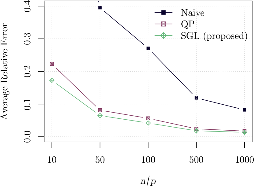
Refer to caption
Refer to caption
Figure 6: Average performance results as, a function of the number of samples, for learning Laplacian matrix of a 4-component graph. The SGL method demonstrates good performance for multi-component graph learning, and significantly outperforms the baseline approaches Naive and QP.

6.3.4 Multi-component graph: noisy setting

Here we aim to learn a multi-component graph under noisy setting. At first we generate a 4 component graph 𝒢mc(20,4,1)subscript𝒢mc2041{\mathcal{G}}_{\textsf{mc}}(20,4,1) with equal number of nodes in all the components, the nodes inside a component are fully connected and the edges are drawn randomly uniformly from [0,1]01[0,1]. Then we add random noise to all the in-component and out component edges. The noise is an Erdos-Renyi graph 𝒢𝖤𝖱(p,)subscript𝒢𝖤𝖱𝑝Weierstrass-p\mathcal{G}_{\mathsf{ER}}(p,\wp), where p=20𝑝20p=20 is the number of nodes, =0.35Weierstrass-p0.35\wp=0.35 is the probability of having an edge between any two pair of nodes, and edge weights are randomly uniformly drawn from [0,κ]0𝜅[0,\kappa]. Specifically, we consider a scenario where each sample 𝐱i𝒩(𝟎,Θ𝗇𝗈𝗂𝗌𝗒)similar-tosubscript𝐱𝑖𝒩0superscriptsubscriptΘ𝗇𝗈𝗂𝗌𝗒{\mathbf{x}}_{i}\sim\mathcal{N}({\mathbf{0}},{{\Theta}}_{\mathsf{noisy}}^{\dagger}) used for calculating SCM as in (117) is drawn from the noisy precision matrix,

Θ𝗇𝗈𝗂𝗌𝗒=Θ𝗍𝗋𝗎𝖾+Θ𝖤𝖱,subscriptΘ𝗇𝗈𝗂𝗌𝗒subscriptΘ𝗍𝗋𝗎𝖾subscriptΘ𝖤𝖱\displaystyle{{\Theta}}_{\mathsf{noisy}}={{\Theta}}_{\mathsf{true}}+{{\Theta}}_{\mathsf{ER}}, (119)

where Θ𝗍𝗋𝗎𝖾subscriptΘ𝗍𝗋𝗎𝖾{{\Theta}}_{\mathsf{true}} is the true Laplacian matrix and Θ𝖤𝖱subscriptΘ𝖤𝖱{{\Theta}}_{\mathsf{ER}} is the noise Laplacian matrix, which follows the ER graph structure. Figure 7 illustrates an instance of the SGL performance for noisy-multi component graph with fixed n/p=30𝑛𝑝30n/p=30, β=400𝛽400\beta=400, α=0.1𝛼0.1\alpha=0.1, and κ=0.45𝜅0.45\kappa=0.45.

Refer to caption
(a) ΘtruesubscriptΘtrue\Theta_{\textsf{true}}
Refer to caption
(b) ΘnoisysubscriptΘnoisy\Theta_{\textsf{noisy}}
Refer to caption
(c) ΘlearnedsubscriptΘlearned\Theta_{\textsf{learned}}
Refer to caption
(d) 𝒢truesubscript𝒢true{\mathcal{G}}_{\textsf{true}}
Refer to caption
(e) 𝒢noisysubscript𝒢noisy{\mathcal{G}}_{\textsf{noisy}}
Refer to caption
(f) 𝒢learnedsubscript𝒢learned{\mathcal{G}}_{\textsf{learned}}
Figure 7: An example of estimating a 4-component graph. Heat maps of the graph matrices: (a) the ground truth graph Laplacian matrix Θ𝗍𝗋𝗎𝖾subscriptΘ𝗍𝗋𝗎𝖾{{\Theta}}_{\mathsf{true}}, (b) Θ𝗇𝗈𝗂𝗌𝗒subscriptΘ𝗇𝗈𝗂𝗌𝗒{{\Theta}}_{\mathsf{noisy}} after being corrupted by noise, (c) ΘlearnedsubscriptΘlearned\Theta_{\textsf{learned}} the learned graph Laplacian with a performance of (𝖱𝖤,𝖥𝖲)=(0.210,1)𝖱𝖤𝖥𝖲0.2101(\mathsf{RE},\mathsf{FS})=(0.210,1), which means a perfect structure recovery even in a noisy setting that heavily suppresses the ground truth weights. The panels (d), (e), and (f) correspond to the graphs represented by the Laplacian matrices in (a), (b), and (c), respectively.

6.3.5 Multi-component graph: components number mismatch

For learning a multi-component graph structure, SGL requires the knowledge of the number of components k𝑘k, as a prior information, which is a common assumption for similar frameworks. If not available, one can infer k𝑘k by using existing methods for model selection e.g., cross validation, Bayesian information criteria (BIC), or Akaike information criteria (AIC). Furthermore, we also investigate the performance when accurate information about the true number of clusters is not available.

We consider an experiment involving model mismatch: the underlying Laplacian matrix that generates the data has j𝑗j number of components but we actually use k𝑘k, kj𝑘𝑗k\neq j, number of components to estimate it. We generate a k=7𝑘7k=7 multi-component graph 𝒢mc(49,7,1)subscript𝒢mc4971{\mathcal{G}}_{\textsf{mc}}(49,7,1), the edge weights are randomly uniformly are drawn from [0,1]01[0,1]. Additionally, we consider a noisy model as in (119) i.e., Θ𝗇𝗈𝗂𝗌𝗒=Θ𝗍𝗋𝗎𝖾+Θ𝖤𝖱subscriptΘ𝗇𝗈𝗂𝗌𝗒subscriptΘ𝗍𝗋𝗎𝖾subscriptΘ𝖤𝖱{{\Theta}}_{\mathsf{noisy}}={{\Theta}}_{\mathsf{true}}+{{\Theta}}_{\mathsf{ER}}, where the noise is an Erdos-Renyi graph 𝒢𝖤𝖱(49,0.25)subscript𝒢𝖤𝖱490.25\mathcal{G}_{\mathsf{ER}}(49,0.25) with edge randomly uniformly drawn from [0,0.45]00.45[0,0.45]. Figure 8 shows an example where the underlying graph has seven components, and we apply the SGL algorithm with j=2𝑗2j=2. As we can see, even though the number of components is mismatched and the data is noisy, the SGL algorithm is still able to identify the true structure with a reasonable performance in terms of F-score and average relative error. The take away from Figure 8 is that, even in the lack of true information regarding the number of components in a graph, the graph learned from the SGL algorithm can yield an initial approximate graph very close to the true graph, which can be used as an input to other algorithms for post-processing to infer more accurate graph.
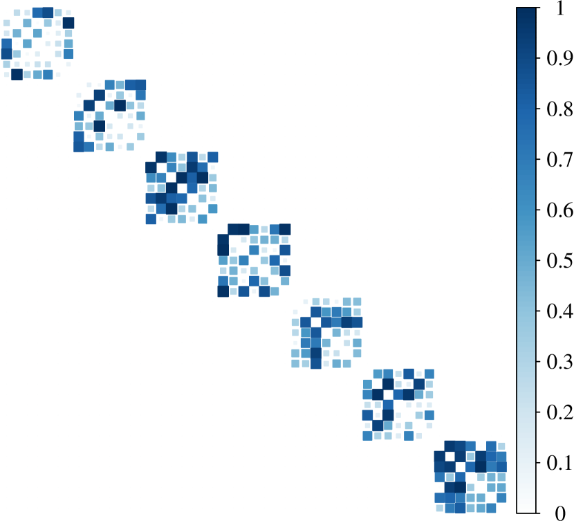
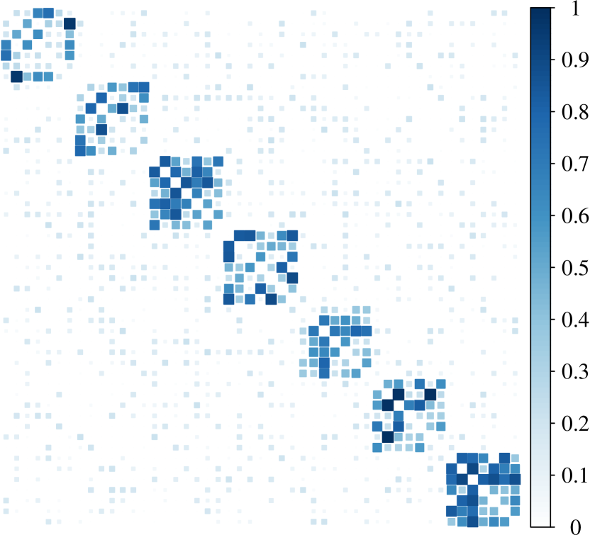
Refer to caption
(a) ΘtruesubscriptΘtrue\Theta_{\textsf{true}} with k=7𝑘7k=7
Refer to caption
(b) ΘnoisysubscriptΘnoisy\Theta_{\textsf{noisy}}
Refer to caption
(c) ΘlearnedsubscriptΘlearned\Theta_{\textsf{learned}} with k=2𝑘2k=2
Refer to caption
(d) 𝒢truesubscript𝒢true{\mathcal{G}}_{\textsf{true}} with k=7𝑘7k=7
Refer to caption
(e) 𝒢noisysubscript𝒢noisy{\mathcal{G}}_{\textsf{noisy}}
Refer to caption
(f) 𝒢learnedsubscript𝒢learned{\mathcal{G}}_{\textsf{learned}} with k=2𝑘2k=2
Figure 8: Heat maps of the graph matrices: (a) the ground truth graph Laplacian of a seven-component graph Θ𝗍𝗋𝗎𝖾subscriptΘ𝗍𝗋𝗎𝖾{{\Theta}}_{\mathsf{true}}, (b) Θ𝗇𝗈𝗂𝗌𝗒subscriptΘ𝗇𝗈𝗂𝗌𝗒{{\Theta}}_{\mathsf{noisy}} after being corrupted by noise, (c) Θ𝗅𝖾𝖺𝗋𝗇𝖾𝖽subscriptΘ𝗅𝖾𝖺𝗋𝗇𝖾𝖽{{\Theta}}_{\mathsf{learned}} the learned graph Laplacian with a performance of (𝖱𝖤,𝖥𝖲)=(0.18,0.81)𝖱𝖤𝖥𝖲0.180.81(\mathsf{RE},\mathsf{FS})=(0.18,0.81). The panels (d), (e), and (f) correspond to the graphs represented by the Laplacian matrices in (a), (b), and (c), respectively. For Figure 8 (c) and (f) we are essentially getting results corresponding to a two-component graph, which is imperative from the usage of spectral constraints of k=2𝑘2k=2. It is observed that the true graph (d) with k=7𝑘7k=7 components are contained exactly in the learned graph (f), the extra edges, which are due to the inaccurate spectral information when removed from 8 (f) can yield the true graph. One can use some simple post-processing techniques (e.g., thresholding of elements in the learned matrix ΘΘ\Theta), to recover the true component structure.
Refer to caption
Figure 9: Average performance results as a function of the number of components k𝑘k: best results are obtained for true number of components. As we can note, the performance is monotonically increasing and eventually reaches a perfect F-score when k=7𝑘7k=7.

Figure 9 depicts the average performance of SGL as a function of k𝑘k. The settings for the experiment is same as in Figure 8, except now we use different number of components information for each instances. It is observed that the SGL has its best performance when k𝑘k matches with the true number of the components in the graph. This also suggests that the SGL algorithm has the potential to be seamlessly integrated with model selection techniques to dynamically determine the number of clusters to use, in a single algorithm (Figueiredo and Jain, 2002; Schaeffer, 2007; Fraley and Raftery, 2007).

6.3.6 Popular multi-component structures

Here we consider the classical problem of clustering for some popular synthetic structures. To do that, we generate 100 nodes per cluster distributed according to structures colloquially known as two moons, two circles, three spirals, three circles, worms and helix 3d. Figure 10 depicts the results of learning the clusters structures using the proposed algorithm SGL.
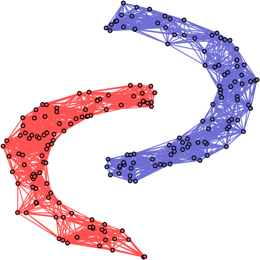
Refer to caption
(a) two moons
Refer to caption
(b) two circles
Refer to caption
(c) three spirals
Refer to caption
(d) three circles
Refer to caption
(e) worms
Refer to caption
(f) helix 3d
Figure 10: SGL is able to perfectly classify the data points according to the cluster membership for all the structures.

6.3.7 Real data: animals data set

Herein, animals data set (Osherson et al., 1991; Lake and Tenenbaum, 2010) is taken into consideration to learn weighted graphs. Graph vertices denote animals, and edge weights representing similarity among them. The data set consists of binary values (categorical non-Gaussian data) which are the answers to questions such as “is warm-blooded?,” “has lungs?”, etc. There are a total of 102 such questions, which make up the features for 33 animal categories. Figure 11 shows the results of estimating the graph of the animals data set using the SGL algorithm with β=1/2𝛽12\beta=1/2 and α=0𝛼0\alpha=0, GGL with α=0.05𝛼0.05\alpha=0.05 and GLasso α=0.05𝛼0.05\alpha=0.05. The input for all the algorithms is the sample covariance matrix plus an identity matrix scaled by 1/3131/3 (see Egilmez et al. (2017)). The evaluation of the estimated graphs is based on the visual inspection. It is expected that similar animals such as (ant, cockroach), (bee, butterfly), and (trout, salmon) would be grouped together. Based on this premise, it can be seen that the SGL algorithm yields a more clear graph than the ones learned by GGL and GLasso.
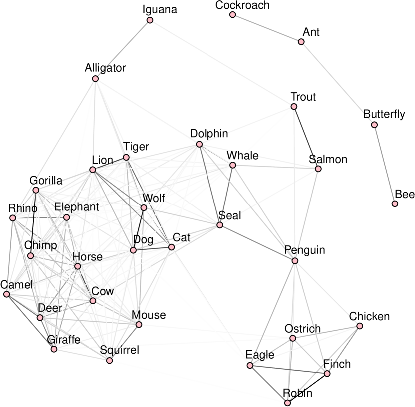
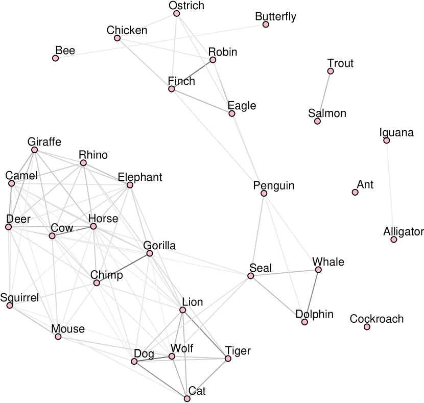
Refer to caption
(a) GLasso(Friedman et al., 2008)
Refer to caption
(b) GGL(Egilmez et al., 2017)
Refer to caption
(c) SGL with k=1𝑘1k=1(proposed)
Refer to caption
(d) SGL with k=5𝑘5k=5(proposed)
Figure 11: Learning the connectivity of the animals data set with (a) GLasso, (b)GGL, (c) SGL with k=1𝑘1k=1 and (d) SGL with k=5𝑘5k=5. All methods obtain perceptual graphs of animal connections: darker edges denote stronger connections among animals. The methods (a) GGL, (b) GLasso, and (c) SGL k=1𝑘1k=1 were expected to obtain sparse-connected graphs. But, GGL, GLasso split the graph into multiple components due to the sparsity regularization. While SGL using sparsity regularization along with spectral constraint k=1𝑘1k=1(connectedness) yields a sparse-connected graph. (d) SGL with k=5𝑘5k=5 obtains a graph with component which depicts a more fine-grained representation of animal connection by grouping similar animals in respective components, highlighting the fact that the explicit control of the number of components may yield an improved visualization. Furthermore, the animal data is categorical (non-Gaussian) which does not follow the IGMRF assumption, the above result also establishes the capability of SGL under mismatch of the data model.

Figure 12 compares the clustering performance of the SGL method for k=10𝑘10k=10 clusters against the state-of-the-art clustering algorithms: (a) klimit-from𝑘k-means clustering, (b) spectral clustering 444 Code for spectral and klimit-from𝑘k-means is available at https://cran.r-project.org/web/packages/kernlab (Karatzoglou et al., 2004), (c) CLR, and (d) SGL with k=10𝑘10k=10. It is remarked that all the algorithms except the SGL are designed only for clustering (grouping) task and are not capable of specifying further connectivity inside a group while SGL is capable of doing both the task of clustering and connectivity(edge weights) estimation jointly.

Refer to caption
(a) klimit-from𝑘k-means
Refer to caption
(b) Spectral (Ng et al., 2002)
Refer to caption
(c) CLR (Nie et al., 2016)
Refer to caption
(d) SGL with k=10𝑘10k=10(proposed)
Figure 12: All the methods obtain 10 components intending to group similar animals together. Clustering with klimit-from𝑘k-means and spectral methods yield components with un-common(possibly wrong) groupings. For example, in (a) seal, cow, horse are grouped together: characteristics of seal does not seem to fit with the cow and horse, and in (b) cockroach, lion, iguana, tiger, ant, alligator are grouped together which is also in contrary to the expectation. On the other hand, it is observed that both CLR (c) and SGL (d) are able to obtain groupings of animal adhering to our general expectation of the animal behaviors. Although both the results vary slightly, the final results from both the methods are meaningful. For example, CLR groups all the insects (bee, butterfly, cockroach, ant) together in one group while SGL splits them into two groups, one with ant, cockroach and another with bee, butterfly. On the other hand, SGL groups the herbivore mammals (horse, elephant, giraffe, deer, camel, rhino, cow) together in one group, while CLR splits these animals into two groups, one containing rhino, elephant and another group containing the rest.

6.3.8 Real data: Cancer Genome data set

For a big-data application, we consider the RNA-Seq Cancer Genome Atlas Research Network (Weinstein et al., 2013) data set available at the UC-Irvine Machine Learning Database (Dheeru and Karra Taniskidou, 2017). This data set consists of genetic features which map 5 types of cancer namely: breast carcinoma (BRCA), kidney renal clear-cell carcinoma (KIRC), lung adenocarcinoma (LUAD), colon adenocarcinoma (COAD), and prostate adenocarcinoma (PRAD). In Figure 13, they are labeled with colors555Please see the plots in color version, black, blue, red, violet, and green, respectively. The data set consists of 801 labeled samples, in which every sample has 20531 genetic features. An important goal with this data set is to classify and group the samples, according to their tumor type, on the basis of those genetic features. We apply the SGL for k=5,β=5formulae-sequence𝑘5𝛽5k=5,\beta=5 algorithm that exploits the spectral constraints to obtain 555 component graph structure: we do not consider the label information.

We also compare the SGL performance against the existing state-of-the-art methods for graph learning algorithms namely GLasso with α=1.71𝛼1.71\alpha=1.71 and GGL with α=1.71𝛼1.71\alpha=1.71 algorithms, and also with the graph-based clustering algorithm CLR with m=10𝑚10m=10, where m𝑚m is the number of neighbors taken into the consideration for creating affinity matrix. We also conducted CLR experiments with different choices of m=3,5,7𝑚357m=3,5,7, and we observed similar performances666The authors in Nie et al. (2016) report that the CLR is insensitive with the choice of m𝑚m for all the values of m𝑚m. See Figure 13 GLasso and GGL are not able to enforce component structure and learn a connected graph with many wrong undesirable edges. SGL method outperforms CLR for the clustering task as well, even though the later is a specialized clustering algorithm.

The improved performance of the SGL can be attributed to two main reasons i) SGL is able to estimate the graph structure and weight simultaneously, which is essentially an optimal joint procedure, ii) SGL is able to capture the conditional dependencies (i.e., the precision matrix entries) among nodes which consider a global view of relationships, while the CLR encodes the connectivity via the direct pairwise distances. The conditional dependencies relationships are expected to give improved performance for clustering tasks (Hao et al., 2018). The performance with SGL shows a perfect clustering, which indicates that SGL may be used to perform simultaneous clustering and graph learning.
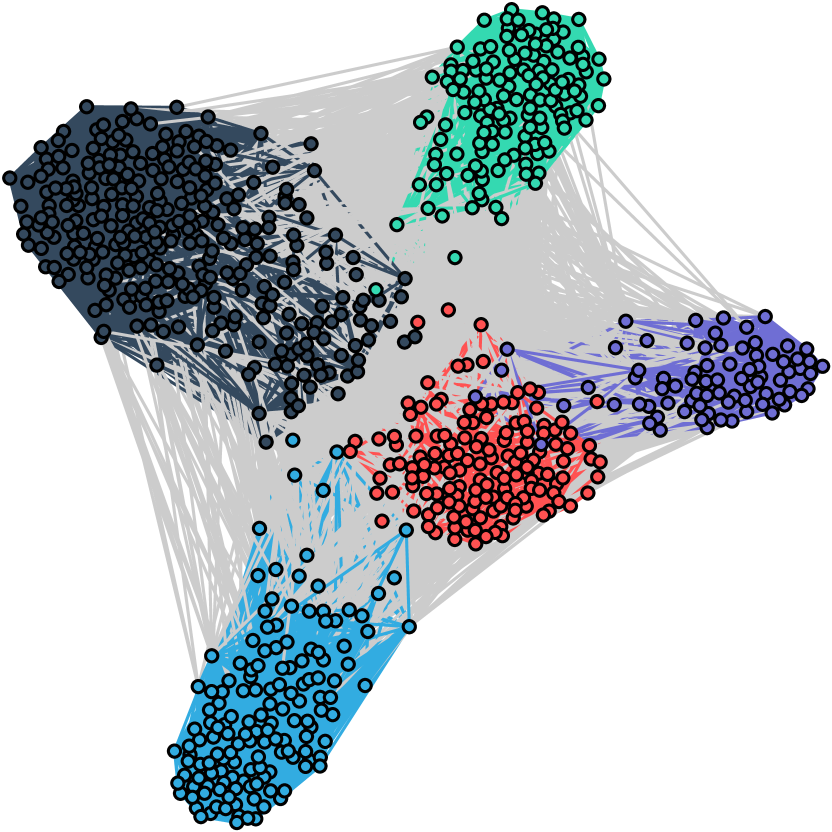
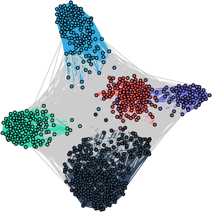
Refer to caption
(a) GLasso(Friedman et al., 2008)
Refer to caption
(b) GGL(Egilmez et al., 2017)
Refer to caption
(c) CLR(Nie et al., 2016)
Refer to caption
(d) SGL(proposed)
Figure 13: Learning the clustered graph for the full 801 genetic samples with 20531 features of the PANCAN data set. Please see the plots in color version. Graph learned with (a) GLasso, (b) GGL method: grey colored edges indicate wrong connections, (c) CLR method: there are two misclassified points in the black group and 10 misclassified points in the red group, and (d) Graph learned with proposed SGL method. Herein, the label information is not taken into consideration. The result for SGL is consistent with the label information: samples belonging to each set are connected together and the components are fairly separated with only few wrongly inter component connections. Furthermore, the graph for the BRCA (black) data sample highlights an inner sub-grouping: suggesting for further biological investigation. This indicates that SGL has the potential to perform both the clustering and multiple graph learning simultaneously.

6.3.9 Effect of the parameter β𝛽\beta

In the current subsection, we study the effect of the parameter β𝛽\beta on the algorithm performance in terms of RE and FS. It is observed from Figure 14 that a large β𝛽\beta enables the SGL to obtain a low RE and a high FS. For a large β𝛽\beta, the formulation puts more weight on the relaxation term so as to make it closer to the spectral constraints. In addition, along with the increase of β𝛽\beta the RE and FS tend to be stable. But empirically it is observed that a huge β𝛽\beta slows down the convergence speed of the algorithm. Similar observations are also made regarding the parameter γ𝛾\gamma for SGA and SGLA algorithms.

Refer to caption
Refer to caption
Figure 14: Effect of the parameter β𝛽\beta on the SGL algorithm. We consider here estimating of a multi-component graph structure 𝒢𝗆𝖼(32,4,0.5)subscript𝒢𝗆𝖼3240.5{\mathcal{G}}_{\mathsf{mc}}(32,4,0.5) edge weights drawn randomly uniformly from [0,1]. It is observed from that a large β𝛽\beta enables the SGL to obtain a low RE and high FS.

6.4 Performance evaluation for SGA Algorithm

A bipartite graph is denoted as 𝒢𝖻𝗂(p1,p2,)subscript𝒢𝖻𝗂subscript𝑝1subscript𝑝2Weierstrass-p{\mathcal{G}}_{\mathsf{bi}}(p_{1},p_{2},\wp), having two disjoint subsets with p1subscript𝑝1p_{1} vertices in one subset and p2subscript𝑝2p_{2} vertices in the another subset, with Weierstrass-p\wp as the probability of having an edge between the nodes of two disjoint subsets. Figure 15 depicts the average performance of the algorithms for different sample size regimes for the following bipartite graph structure 𝒢𝖻𝗂(p1=40,p2=24,=0.6)subscript𝒢𝖻𝗂formulae-sequencesubscript𝑝140formulae-sequencesubscript𝑝224Weierstrass-p0.6{\mathcal{G}}_{\mathsf{bi}}(p_{1}=40,p_{2}=24,\wp=0.6) with edge weights are randomly uniformly selected from [1,3]13[1,3]. We set γ=105𝛾superscript105\gamma=10^{5}. Here we consider a connected bipartite graph, thus SGA is also compared against CGL.
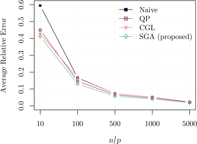
Refer to caption
Refer to caption
Figure 15: Average performance results for learning Laplacian matrix of a bipartite graph structure 𝒢𝖻𝗂subscript𝒢𝖻𝗂\mathcal{G}_{\mathsf{bi}}. The proposed SGA method significantly outperforms the base line approaches, Naive, QP and CGL.

6.4.1 Bipartite graph leaning: noisy setting

We consider here learning of a bipartite graph structure under the noisy setting (119), i.e., the samples used for calculating the SCM is obtained from noisy precision matrix, for which, the ground truth precision matrix corresponds to a bipartite graph. At first we generate 𝒢bi(40,24,0.70)subscript𝒢bi40240.70{\mathcal{G}}_{\textsf{bi}}(40,24,0.70) and the edge weights are drawn from [0.1,1]0.11[0.1,1]. Then we add random noise to all the possible connections, by adding edge weights following the ER graph 𝒢𝖤𝖱(64,0.35)subscript𝒢𝖤𝖱640.35\mathcal{G}_{\mathsf{ER}}(64,0.35) graph model. Figure 16 illustrates an instance of SGA algorithm performance for learning bipartite graph structure from noisy sample data.
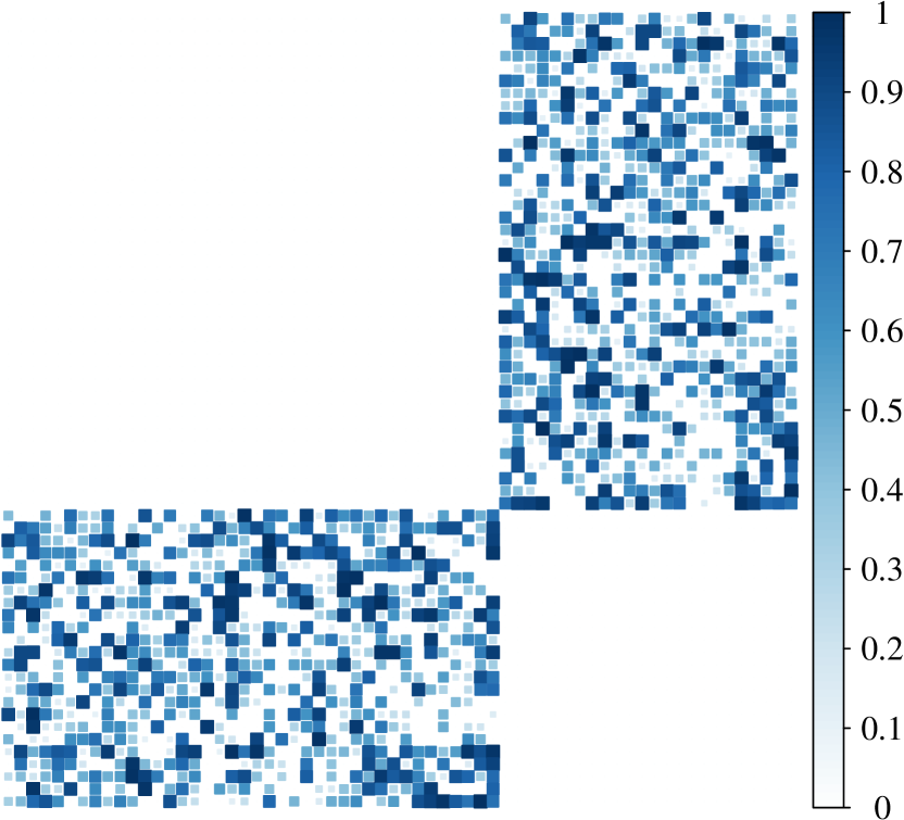
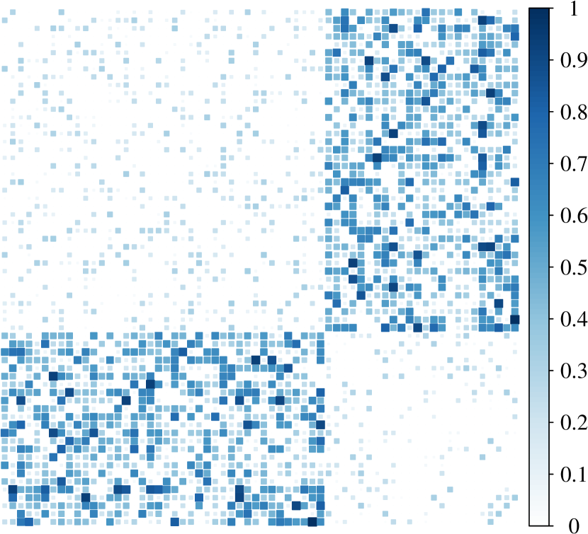
Refer to caption
(a) ΘtruesubscriptΘtrue\Theta_{\textsf{true}}
Refer to caption
(b) ΘnoisysubscriptΘnoisy\Theta_{\textsf{noisy}}
Refer to caption
(c) ΘlearnedsubscriptΘlearned\Theta_{\textsf{learned}}
Figure 16: An instance of bipartite graph learning with SGA algorithm with data generated from noisy graph Laplacian, and fixing n/p=500𝑛𝑝500n/p=500 and γ=105𝛾superscript105\gamma=10^{5}. (a) the ground truth Laplacian matrix (Θ𝗍𝗋𝗎𝖾subscriptΘ𝗍𝗋𝗎𝖾{{\Theta}}_{\mathsf{true}}), (b) Θ𝗇𝗈𝗂𝗌𝗒subscriptΘ𝗇𝗈𝗂𝗌𝗒{{\Theta}}_{\mathsf{noisy}} after being corrupted by noise, (c) the learned graph Laplacian with a performance of (𝖱𝖤=0.219,𝖥𝖲=0.872)formulae-sequence𝖱𝖤0.219𝖥𝖲0.872(\mathsf{RE}=0.219,\mathsf{FS}=0.872).

6.5 Performance evaluation for SGLA Algorithm

Herein, we consider learning of a multi-component bipartite graph structure. This structure is widely used in a lot of applications including medicine and biology (see Nie et al., 2017; Pavlopoulos et al., 2018), which makes it appealing from both the practical as well as theoretical and algorithmic perspective. To learn multi-component bipartite graph structure from the SCM of data S𝑆S, we plugin the Laplacian spectral properties (𝒮λsubscript𝒮𝜆{\mathcal{S}}_{\lambda} as in (18)) corresponding to the multi-component structure along with the adjacency spectral constraints corresponding to the bipartite structure (i.e., 𝒮ψsubscript𝒮𝜓{\mathcal{S}}_{\psi} as in (28)) in Algorithm 4 [cf. step 8, 9].
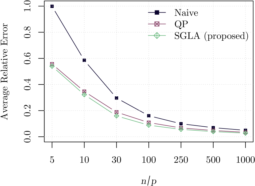
Refer to caption
Refer to caption
Figure 17: Average performance results for learning Laplacian matrix of a 𝒢𝖻𝗂subscript𝒢𝖻𝗂\mathcal{G}_{\mathsf{bi}}. The proposed SGLA method significantly outperforms the base line approaches, QP and Naive.

Figure 17 depicts the average performance of the algorithms for different sample size regimes for a block- bipartite graph structure three components k=3𝑘3k=3 with unequal number of nodes, where each component represents a bipartite graph structure, denoted by 𝒢bi1(20,8,0.5)subscriptsuperscript𝒢1bi2080.5{\mathcal{G}}^{1}_{\textsf{bi}}(20,8,0.5), 𝒢bi2(12,8,0.6)2subscriptsuperscript𝒢2bisuperscript1280.62{\mathcal{G}}^{2}_{\textsf{bi}}(12,8,0.6)^{2}, and 𝒢bi3(8,8,0.7)subscriptsuperscript𝒢3bi880.7{\mathcal{G}}^{3}_{\textsf{bi}}(8,8,0.7), bipartite edge weights are randomly uniformly drawn from [0.1,3]0.13[0.1,3]. We fix β=103𝛽superscript103\beta=10^{3} and γ=103𝛾superscript103\gamma=10^{3}. Here we consider a multi-component bipartite graph, therefore we can only compare against, QP and Naive. In terms of RE, QP performance is comparable with SGLA but in terms of FS, SGLA significantly outperforms the baseline approaches.

6.5.1 Multi-component bipartite graph: noisy setting

We consider here learning of a block-bipartite graph structure under the noisy setting (119), i.e., the samples used for calculating the SCM is obtained from noisy precision matrix, for which, the ground truth precision matrix corresponds to a multi-component bipartite graph. We first generate a graph of p=32𝑝32p=32 nodes and three components k=3𝑘3k=3 with unequal number of nodes, where each component represents a bipartite graph structure, denoted by 𝒢bi1(10,4,0.7)subscriptsuperscript𝒢1bi1040.7{\mathcal{G}}^{1}_{\textsf{bi}}(10,4,0.7), 𝒢bi2(6,4,0.8)2subscriptsuperscript𝒢2bisuperscript640.82{\mathcal{G}}^{2}_{\textsf{bi}}(6,4,0.8)^{2}, and 𝒢bi3(4,4,0.9)subscriptsuperscript𝒢3bi440.9{\mathcal{G}}^{3}_{\textsf{bi}}(4,4,0.9), bipartite edge weights are drawn from [1,3]13[1,3]. Then we add random noise to all the possible edges between any two vertices by adding edge weights following the ER graph 𝒢𝖤𝖱(32,.35)subscript𝒢𝖤𝖱32.35\mathcal{G}_{\mathsf{ER}}(32,.35) with edges drawn from [0,1]01[0,1], and we fix n/p=250𝑛𝑝250n/p=250, γ=105𝛾superscript105\gamma=10^{5} and β=105𝛽superscript105\beta=10^{5}. Figure 18 depicts one instance of the performance of SGLA for noisy bipartite graph structure.
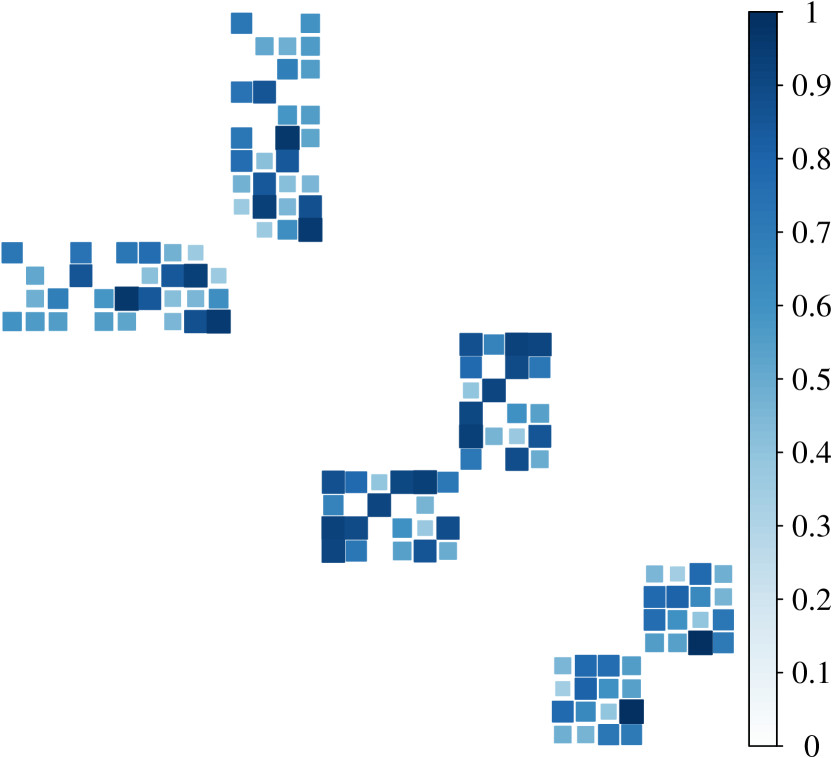
Refer to caption
(a) ΘtruesubscriptΘtrue\Theta_{\textsf{true}}
Refer to caption
(b) ΘnoisysubscriptΘnoisy\Theta_{\textsf{noisy}}
Refer to caption
(c) ΘlearnedsubscriptΘlearned\Theta_{\textsf{learned}}
Figure 18: An example of learning a 3-component bipartite graph structure with SGLA algorithm, the samples used for calculating the SCM is obtained from noisy Laplacian precision matrix. Heat maps of the graph matrices: (a) Θ𝗍𝗋𝗎𝖾subscriptΘ𝗍𝗋𝗎𝖾{{\Theta}}_{\mathsf{true}} the ground truth Laplacian matrix, (b) Θ𝗇𝗈𝗂𝗌𝗒subscriptΘ𝗇𝗈𝗂𝗌𝗒{{\Theta}}_{\mathsf{noisy}} after being corrupted by noise, (c) ΘlearnedsubscriptΘlearned\Theta_{\textsf{learned}} the learned graph Laplacian with a performance of (𝖱𝖤=0.225,𝖥𝖲=0.947)formulae-sequence𝖱𝖤0.225𝖥𝖲0.947(\mathsf{RE}=0.225,\mathsf{FS}=0.947), which means a perfect structure recovery even in a noisy model that heavily suppresses the ground truth weights.

7 Discussion and Conclusion

In this paper, for learning graphs with specific structures, we have considered the spectral constraints on the eigenvalues of graph matrices under the GGM setting. We have developed a unified optimization framework which is very general and putsforth plausible directions for future works.

7.1 Discussion

The extensions of this paper include considering more specific prior information on eigenvalues constraints, obtaining structured graph transform for graph signal processing applications and, extending the framework by considering other statistical models.

7.1.1 Other spectral prior information

In addition to the spectral properties considered in this paper, there are numerous interesting results in the literature relating other properties to some specific graph structures, we refer readers to the comprehensive exposition in (see for Laplacian eigenvalues, Das and Bapat, 2005; Yu and Lu, 2014; Farber and Kaminer, 2011; Berman and Farber, 2011; Chung, 1997; Spielman and Teng, 2011) see (Chung, 1997; Mohar, 1997; Yang et al., 2003; Van Mieghem, 2010; Schulte, 1996; Lin et al., 2014). The proposed framework has the potential to be extended for undertaking those prior spectral information.

7.1.2 Structured statistical models

Although, the focus of the current paper is on the unification of spectral graph theory with the GGM framework, but the proposed spectral constraints and developed algorithms are very general and can be integrated with other statistical models such as structured Ising model (Ravikumar et al., 2010), structured Gaussian covariance graphical models (Drton and Richardson, 2008), structured Gaussian graphical models with latent variables (Chandrasekaran et al., 2010), least-square formulation for graph learning (Nie et al., 2016), structured linear regression, and vector auto-regression models (Basu et al., 2015).

7.1.3 Structured graph signal processing

One of the motivations of the present work comes from Graph signal processing (GSP), which provides a promising tool for the representation, processing and analysis of complex networked-data (e.g., social, energy, finance, biology and, etc.), where the data are defined on the vertices of a graph (Shuman et al., 2013; Ortega et al., 2018). The eigenvector of graph matrices are used to define graph Fourier transform also known as dictionaries, used in a variety applications including, graph-based filtering, graph-based transforms, and sampling for graph signals. More recently it is realized that the graph eigenvectors with additional properties (e.g., sparsity) could be instrumental in doing some complex tasks. For example, sparse eigenvectors of the graph matrices are important to investigate the uncertainty principle over graphs (Teke and Vaidyanathan, 2017). Few other examples include sparsifying eigenvectors (Sardellitti et al., 2018) and robust eigenvectors(Maretic et al., 2017). Within the proposed formulation, one can easily enforce desired properties on the eigenvectors by pairing the optimization step of (27), (35) and (17) with specific constraints on the eigenvectors (e.g., through regularization). Joint learning structured graphs with specific properties on the eigenvectors have significant potential for GSP applications, which have not been investigated yet, and constitute a promising research direction.

7.2 Conclusion

Summarizing, in this paper, we have shown how to convert the combinatorial constraints of structured graph learning into analytical constraints of the graph matrix eigenvalues. We have developed three algorithms SGL, SGA, and SGLA that can learn structured graphs from a large class of graph families. The algorithms are capable of learning the graph structure and their weights simultaneously by utilizing the spectral constraints of graph matrices directly into the Gaussian graphical modeling framework. The algorithms enjoy comprehensive theoretical convergence properties along with low computational complexity. Extensive numerical experiments with both synthetic and real data sets demonstrate the effectiveness of the proposed methods. The paper also puts forth several extensions worthy of possible future research direction.

8 Appendix

8.1 Proof of Lemma 2

Proof.

We define an index set ΩtsubscriptΩ𝑡\Omega_{t}:

Ωt:={l|[𝐱]tt=lΩtxl},t[1,p].formulae-sequenceassignsubscriptΩ𝑡conditional-set𝑙subscriptdelimited-[]𝐱𝑡𝑡subscript𝑙subscriptΩ𝑡subscript𝑥𝑙𝑡1𝑝\displaystyle\Omega_{t}:=\left\{l\ |[{\mathcal{L}}{\mathbf{x}}]_{tt}=\sum_{l\in\Omega_{t}}x_{l}\right\},\quad t\in[1,p]. (120)

For any 𝐱p(p1)2𝐱superscript𝑝𝑝12{\mathbf{x}}\in{\mathbb{R}}^{\frac{p(p-1)}{2}}, we have

𝐱F2superscriptsubscriptnorm𝐱𝐹2\displaystyle\left\|{\mathcal{L}}{\mathbf{x}}\right\|_{F}^{2} =2k=1p(p1)2xk2+i=1p([𝐱]ii)2absent2superscriptsubscript𝑘1𝑝𝑝12superscriptsubscript𝑥𝑘2superscriptsubscript𝑖1𝑝superscriptsubscriptdelimited-[]𝐱𝑖𝑖2\displaystyle=2\sum_{k=1}^{\frac{p(p-1)}{2}}x_{k}^{2}+\sum_{i=1}^{p}([{\mathcal{L}}{\mathbf{x}}]_{ii})^{2} (121)
=4k=1p(p1)2xk2+t=1ni,jΩt,ijxixjabsent4superscriptsubscript𝑘1𝑝𝑝12superscriptsubscript𝑥𝑘2superscriptsubscript𝑡1𝑛subscriptformulae-sequence𝑖𝑗subscriptΩ𝑡𝑖𝑗subscript𝑥𝑖subscript𝑥𝑗\displaystyle=4\sum_{k=1}^{\frac{p(p-1)}{2}}x_{k}^{2}+\sum_{t=1}^{n}\sum_{i,j\in\Omega_{t},\ i\neq j}x_{i}x_{j} (122)
4k=1p(p1)2xk2+12t=1ni,jΩt,ijxi2+xj2absent4superscriptsubscript𝑘1𝑝𝑝12superscriptsubscript𝑥𝑘212superscriptsubscript𝑡1𝑛subscriptformulae-sequence𝑖𝑗subscriptΩ𝑡𝑖𝑗superscriptsubscript𝑥𝑖2superscriptsubscript𝑥𝑗2\displaystyle\leq 4\sum_{k=1}^{\frac{p(p-1)}{2}}x_{k}^{2}+\frac{1}{2}\sum_{t=1}^{n}\sum_{i,j\in\Omega_{t},\ i\neq j}x_{i}^{2}+x_{j}^{2} (123)
=(4+2(|Ωt|1))k=1p(p1)2xk2absent42subscriptΩ𝑡1superscriptsubscript𝑘1𝑝𝑝12superscriptsubscript𝑥𝑘2\displaystyle=(4+2(|\Omega_{t}|-1))\sum_{k=1}^{\frac{p(p-1)}{2}}x_{k}^{2} (124)
=2p𝐱2,absent2𝑝superscriptnorm𝐱2\displaystyle=2p\left\|{\mathbf{x}}\right\|^{2}, (125)

where the second equality is due to the fact that each xksubscript𝑥𝑘x_{k} only appears twice on the diagonal; the first inequality achieves equality when each xksubscript𝑥𝑘x_{k} is equal; the last equality follows the fact that |Ωt|=p1subscriptΩ𝑡𝑝1|\Omega_{t}|=p-1.

Therefore, by the definition of operator norm, we can obtain

2=sup𝐱=1𝐱F=2p,subscriptnorm2subscriptsupremumnorm𝐱1subscriptnorm𝐱𝐹2𝑝\displaystyle\left\|{\mathcal{L}}\right\|_{2}=\sup_{\left\|{\mathbf{x}}\right\|=1}\left\|{\mathcal{L}}{\mathbf{x}}\right\|_{F}=\sqrt{2p}, (126)

concluding the proof.

8.2 Proof for Lemma 7

The Lagrangian of the optimization (74) is

L(𝝀,𝝁)𝐿𝝀𝝁\displaystyle L({\bm{\lambda}},\bm{\mu}) =i=1qlogλi+β2𝝀𝐝22absentsuperscriptsubscript𝑖1𝑞subscript𝜆𝑖𝛽2superscriptsubscriptnorm𝝀𝐝22\displaystyle=-\sum_{i=1}^{q}\log\lambda_{i}+\frac{\beta}{2}\|{\bm{\lambda}}-\mathbf{d}\|_{2}^{2} (127)
+μ1(c1λ1)+i=2qμi(λi1λi)+μq+1(λqc2).subscript𝜇1subscript𝑐1subscript𝜆1superscriptsubscript𝑖2𝑞subscript𝜇𝑖subscript𝜆𝑖1subscript𝜆𝑖subscript𝜇𝑞1subscript𝜆𝑞subscript𝑐2\displaystyle+\mu_{1}(c_{1}-\lambda_{1})+\sum_{i=2}^{q}\mu_{i}(\lambda_{i-1}-\lambda_{i})+\mu_{q+1}(\lambda_{q}-c_{2}).

The KKT optimality conditions are derived as:

1λi+β(λidi)μi+μi+11subscript𝜆𝑖𝛽subscript𝜆𝑖subscript𝑑𝑖subscript𝜇𝑖subscript𝜇𝑖1\displaystyle-\frac{1}{\lambda_{i}}+\beta(\lambda_{i}-d_{i})-\mu_{i}+\mu_{i+1} =0,i=1,,q;formulae-sequenceabsent0𝑖1𝑞\displaystyle=0,\ i=1,\cdots,q; (128)
c1λ1subscript𝑐1subscript𝜆1\displaystyle c_{1}-\lambda_{1} 0;absent0\displaystyle\leq 0; (129)
λi1λisubscript𝜆𝑖1subscript𝜆𝑖\displaystyle\lambda_{i-1}-\lambda_{i} 0,i=2,,q;formulae-sequenceabsent0𝑖2𝑞\displaystyle\leq 0,\ i=2,\cdots,q; (130)
λqc2subscript𝜆𝑞subscript𝑐2\displaystyle\lambda_{q}-c_{2} 0;absent0\displaystyle\leq 0; (131)
μisubscript𝜇𝑖\displaystyle\mu_{i} 0,i=1,,q+1;formulae-sequenceabsent0𝑖1𝑞1\displaystyle\geq 0,\ i=1,\cdots,q+1; (132)
μ1(c1λ1)subscript𝜇1subscript𝑐1subscript𝜆1\displaystyle\mu_{1}(c_{1}-\lambda_{1}) =0;absent0\displaystyle=0; (133)
μi(λi1λi)subscript𝜇𝑖subscript𝜆𝑖1subscript𝜆𝑖\displaystyle\mu_{i}(\lambda_{i-1}-\lambda_{i}) =0,i=2,,q;formulae-sequenceabsent0𝑖2𝑞\displaystyle=0,\ i=2,\cdots,q; (134)
μq+1(λqc2)subscript𝜇𝑞1subscript𝜆𝑞subscript𝑐2\displaystyle\mu_{q+1}(\lambda_{q}-c_{2}) =0;absent0\displaystyle=0; (135)
Lemma 18.

The solution of the KKT system (128)-(135) is λi=(di+di2+4/β)/2subscript𝜆𝑖subscript𝑑𝑖superscriptsubscript𝑑𝑖24𝛽2\lambda_{i}=(d_{i}+\sqrt{d_{i}^{2}+4/\beta})/2, for i=1,,q𝑖1𝑞i=1,\cdots,q, if c1λ1cqc2subscript𝑐1subscript𝜆1subscript𝑐𝑞subscript𝑐2c_{1}\leq\lambda_{1}\leq\cdots\leq c_{q}\leq c_{2} hold.

Proof.

It is obvious that it conditions c1λ1λqc2subscript𝑐1subscript𝜆1subscript𝜆𝑞subscript𝑐2c_{1}\leq\lambda_{1}\leq\cdots\leq\lambda_{q}\leq c_{2} hold, then the solutions of the primal and dual variables satisfy all equations. ∎

We start from the corresponding unconstrained version of the problem (74) whose solution is

λi(0)=(di+di2+4/β)/2.superscriptsubscript𝜆𝑖0subscript𝑑𝑖superscriptsubscript𝑑𝑖24𝛽2\displaystyle\lambda_{i}^{(0)}=\left(d_{i}+\sqrt{d_{i}^{2}+4/\beta}\right)/2. (136)

If this solution satisfies all the KKT conditions (128)-(135), then it is also the optimal. Otherwise, each λi(0)superscriptsubscript𝜆𝑖0\lambda_{i}^{(0)} that violates the conditions c1λ1(0)λq(0)c2subscript𝑐1superscriptsubscript𝜆10superscriptsubscript𝜆𝑞0subscript𝑐2c_{1}\leq\lambda_{1}^{(0)}\leq\cdots\leq\lambda_{q}^{(0)}\leq c_{2} needs to be updated.

Situation 1: c1λ1(0)λr(0)subscript𝑐1superscriptsubscript𝜆10superscriptsubscript𝜆𝑟0c_{1}\geq\lambda_{1}^{(0)}\geq\cdots\geq\lambda_{r}^{(0)}, implying c11c1βd1drsubscript𝑐11subscript𝑐1𝛽subscript𝑑1subscript𝑑𝑟c_{1}-\frac{1}{c_{1}\beta}\geq d_{1}\geq\cdots\geq d_{r}, where at least one inequality is strict and r1𝑟1r\geq 1. Without loss of generality, let the j𝑗j-th inequality is strict with 1jr1𝑗𝑟1\leq j\leq r, i.e. dj>dj+1subscript𝑑𝑗subscript𝑑𝑗1d_{j}>d_{j+1}. The KKT optimality conditions for this pare are:

1λj+β(λjdj)μj+μj+11subscript𝜆𝑗𝛽subscript𝜆𝑗subscript𝑑𝑗subscript𝜇𝑗subscript𝜇𝑗1\displaystyle-\frac{1}{\lambda_{j}}+\beta(\lambda_{j}-d_{j})-\mu_{j}+\mu_{j+1} =0;absent0\displaystyle=0; (137)
1λj+1+β(λj+1dj+1)μj+1+μj+21subscript𝜆𝑗1𝛽subscript𝜆𝑗1subscript𝑑𝑗1subscript𝜇𝑗1subscript𝜇𝑗2\displaystyle-\frac{1}{\lambda_{j+1}}+\beta(\lambda_{j+1}-d_{j+1})-\mu_{j+1}+\mu_{j+2} =0;absent0\displaystyle=0; (138)
λjλj+1subscript𝜆𝑗subscript𝜆𝑗1\displaystyle\lambda_{j}-\lambda_{j+1} 0;absent0\displaystyle\leq 0; (139)
μisubscript𝜇𝑖\displaystyle\mu_{i} 0,i=j,j+1,j+2;formulae-sequenceabsent0𝑖𝑗𝑗1𝑗2\displaystyle\geq 0,\ i=j,j+1,j+2; (140)
μj+1(λjλj+1)subscript𝜇𝑗1subscript𝜆𝑗subscript𝜆𝑗1\displaystyle\mu_{j+1}(\lambda_{j}-\lambda_{j+1}) =0;absent0\displaystyle=0; (141)

We subtract the first two equations and obtain:

2μj+1=μj+2+μj+(1λj1λj+1)+β(λj+1λj)+β(djdj+1)>0,2subscript𝜇𝑗1subscript𝜇𝑗2subscript𝜇𝑗1subscript𝜆𝑗1subscript𝜆𝑗1𝛽subscript𝜆𝑗1subscript𝜆𝑗𝛽subscript𝑑𝑗subscript𝑑𝑗10\displaystyle 2\mu_{j+1}=\mu_{j+2}+\mu_{j}+(\frac{1}{\lambda_{j}}-\frac{1}{\lambda_{j+1}})+\beta(\lambda_{j+1}-\lambda_{j})+\beta(d_{j}-d_{j+1})>0, (142)

due to the fact that dj>dj+1subscript𝑑𝑗subscript𝑑𝑗1d_{j}>d_{j+1} and λjλj+1subscript𝜆𝑗subscript𝜆𝑗1\lambda_{j}\leq\lambda_{j+1}. Since μj+1>0subscript𝜇𝑗10\mu_{j+1}>0, we also have

2μj=μj+1+μj1+(1λj11λj)+β(λjλj1)+β(dj1dj)>0,2subscript𝜇𝑗subscript𝜇𝑗1subscript𝜇𝑗11subscript𝜆𝑗11subscript𝜆𝑗𝛽subscript𝜆𝑗subscript𝜆𝑗1𝛽subscript𝑑𝑗1subscript𝑑𝑗0\displaystyle 2\mu_{j}=\mu_{j+1}+\mu_{j-1}+(\frac{1}{\lambda_{j-1}}-\frac{1}{\lambda_{j}})+\beta(\lambda_{j}-\lambda_{j-1})+\beta(d_{j-1}-d_{j})>0, (143)

where dj1djsubscript𝑑𝑗1subscript𝑑𝑗d_{j-1}\geq d_{j} and λj1λjsubscript𝜆𝑗1subscript𝜆𝑗\lambda_{j-1}\leq\lambda_{j}. Similarly, we can obtain μj>0subscript𝜇𝑗0\mu_{j}>0 with 2jr2𝑗𝑟2\leq j\leq r. In addition,

μ1subscript𝜇1\displaystyle\mu_{1} =1λ1+β(λ1d1)+μ2absent1subscript𝜆1𝛽subscript𝜆1subscript𝑑1subscript𝜇2\displaystyle=-\frac{1}{\lambda_{1}}+\beta(\lambda_{1}-d_{1})+\mu_{2} (144)
1c1+β(c1d1)+μ2>0.1subscript𝑐1𝛽subscript𝑐1subscript𝑑1subscript𝜇20\displaystyle-\frac{1}{c_{1}}+\beta(c_{1}-d_{1})+\mu_{2}>0. (145)

Totally, we have μj>0subscript𝜇𝑗0\mu_{j}>0 with 1jr1𝑗𝑟1\leq j\leq r. By (133) and (134), we obtain λ1==λr=c1subscript𝜆1subscript𝜆𝑟subscript𝑐1\lambda_{1}=\cdots=\lambda_{r}=c_{1}. Therefore, we update

λ1(1)==λr(1)=c1.superscriptsubscript𝜆11superscriptsubscript𝜆𝑟1subscript𝑐1\displaystyle\lambda_{1}^{(1)}=\cdots=\lambda_{r}^{(1)}=c_{1}. (146)

Situation 2: λs(0)λq(0)c2superscriptsubscript𝜆𝑠0superscriptsubscript𝜆𝑞0subscript𝑐2\lambda_{s}^{(0)}\geq\cdots\geq\lambda_{q}^{(0)}\geq c_{2}, implying dsdqc21c2βsubscript𝑑𝑠subscript𝑑𝑞subscript𝑐21subscript𝑐2𝛽d_{s}\geq\cdots\geq d_{q}\geq c_{2}-\frac{1}{c_{2}\beta}, where at least one inequality is strict and sq𝑠𝑞s\leq q.

Similar to situation 1, we can also obtain μj>0subscript𝜇𝑗0\mu_{j}>0 with s+1jm+1𝑠1𝑗𝑚1s+1\leq j\leq m+1 and thus λs==λq=c2subscript𝜆𝑠subscript𝜆𝑞subscript𝑐2\lambda_{s}=\cdots=\lambda_{q}=c_{2}. Therefore, we update λs(0),,λq(0)superscriptsubscript𝜆𝑠0superscriptsubscript𝜆𝑞0\lambda_{s}^{(0)},\cdots,\lambda_{q}^{(0)} by λs(1)==λq(1)=c2superscriptsubscript𝜆𝑠1superscriptsubscript𝜆𝑞1subscript𝑐2\lambda_{s}^{(1)}=\cdots=\lambda_{q}^{(1)}=c_{2}.

Situation 3: λi(0)λm(0)superscriptsubscript𝜆𝑖0superscriptsubscript𝜆𝑚0\lambda_{i}^{(0)}\geq\cdots\geq\lambda_{m}^{(0)}, implying didmsubscript𝑑𝑖subscript𝑑𝑚d_{i}\geq\cdots\geq d_{m}, where at least one inequality is strict and 1imq1𝑖𝑚𝑞1\leq i\leq m\leq q. Here we assume λi1(0)<λi(0)superscriptsubscript𝜆𝑖10superscriptsubscript𝜆𝑖0\lambda_{i-1}^{(0)}<\lambda_{i}^{(0)} (c1<λ1(0)subscript𝑐1superscriptsubscript𝜆10c_{1}<\lambda_{1}^{(0)} if i=1𝑖1i=1) and λm(0)<λm+1(0)superscriptsubscript𝜆𝑚0superscriptsubscript𝜆𝑚10\lambda_{m}^{(0)}<\lambda_{m+1}^{(0)} (λq(0)<c2superscriptsubscript𝜆𝑞0subscript𝑐2\lambda_{q}^{(0)}<c_{2} if m=q𝑚𝑞m=q). Otherwise, this will be reduced to situation 1 or 3.

Similar to situation 1, we can also obtain μj>0subscript𝜇𝑗0\mu_{j}>0 with i+1jm𝑖1𝑗𝑚i+1\leq j\leq m and thus λi(1)=λi+1(1)==λm(1)superscriptsubscript𝜆𝑖1superscriptsubscript𝜆𝑖11superscriptsubscript𝜆𝑚1\lambda_{i}^{(1)}=\lambda_{i+1}^{(1)}=\cdots=\lambda_{m}^{(1)}.

We sum up equations (137) with ijm𝑖𝑗𝑚i\leq j\leq m and obtain

1λj+βλj1mi+1(βj=imdj+μiμm+1)=0,j=i,,m.formulae-sequence1subscript𝜆𝑗𝛽subscript𝜆𝑗1𝑚𝑖1𝛽superscriptsubscript𝑗𝑖𝑚subscript𝑑𝑗subscript𝜇𝑖subscript𝜇𝑚10𝑗𝑖𝑚\displaystyle-\frac{1}{\lambda_{j}}+\beta\lambda_{j}-\frac{1}{m-i+1}(\beta\sum_{j=i}^{m}d_{j}+\mu_{i}-\mu_{m+1})=0,\quad j=i,\cdots,m. (147)

Here we need to use iterative method to find the solution that satisfies KKT conditions. It is easy to check that μi=μm+1=0subscript𝜇𝑖subscript𝜇𝑚10\mu_{i}=\mu_{m+1}=0 when λi1(0)<λi(0)superscriptsubscript𝜆𝑖10superscriptsubscript𝜆𝑖0\lambda_{i-1}^{(0)}<\lambda_{i}^{(0)} and λm(0)<λm+1(0)superscriptsubscript𝜆𝑚0superscriptsubscript𝜆𝑚10\lambda_{m}^{(0)}<\lambda_{m+1}^{(0)}. In that case, according to (147), we have

λj=(d¯im+d¯im2+4/β)/2,j=i,,m.formulae-sequencesubscript𝜆𝑗subscript¯𝑑𝑖𝑚subscriptsuperscript¯𝑑2𝑖𝑚4𝛽2𝑗𝑖𝑚\displaystyle\lambda_{j}=\left(\bar{d}_{i\to m}+\sqrt{\bar{d}^{2}_{i\to m}+4/\beta}\right)/2,\quad j=i,\cdots,m. (148)

where d¯im=1mi+1j=imdjsubscript¯𝑑𝑖𝑚1𝑚𝑖1superscriptsubscript𝑗𝑖𝑚subscript𝑑𝑗\bar{d}_{i\to m}=\frac{1}{m-i+1}\sum_{j=i}^{m}d_{j}. Therefore, we update λi(0),,λm(0)superscriptsubscript𝜆𝑖0superscriptsubscript𝜆𝑚0\lambda_{i}^{(0)},\cdots,\lambda_{m}^{(0)} by

λi(1)==λm(1)=(d¯im+d¯im2+4/β)/2.superscriptsubscript𝜆𝑖1superscriptsubscript𝜆𝑚1subscript¯𝑑𝑖𝑚subscriptsuperscript¯𝑑2𝑖𝑚4𝛽2\displaystyle\lambda_{i}^{(1)}=\cdots=\lambda_{m}^{(1)}=\left(\bar{d}_{i\to m}+\sqrt{\bar{d}^{2}_{i\to m}+4/\beta}\right)/2. (149)

If there exists the case that λi1(1)>λi(1)superscriptsubscript𝜆𝑖11superscriptsubscript𝜆𝑖1\lambda_{i-1}^{(1)}>\lambda_{i}^{(1)}, we need to further update λi1(1),λi(1),,λm(1)superscriptsubscript𝜆𝑖11superscriptsubscript𝜆𝑖1superscriptsubscript𝜆𝑚1\lambda_{i-1}^{(1)},\lambda_{i}^{(1)},\cdots,\lambda_{m}^{(1)} in the next iteration. It will include two cases to discuss:

1. λi1(1)superscriptsubscript𝜆𝑖11\lambda_{i-1}^{(1)} has not been updated by (149), implying that λi1(1)=λi1(0)=(d¯i1+di12+4/β)/2superscriptsubscript𝜆𝑖11superscriptsubscript𝜆𝑖10subscript¯𝑑𝑖1subscriptsuperscript𝑑2𝑖14𝛽2\lambda_{i-1}^{(1)}=\lambda_{i-1}^{(0)}=\left(\bar{d}_{i-1}+\sqrt{d^{2}_{i-1}+4/\beta}\right)/2. So λi1(1)>λi(1)superscriptsubscript𝜆𝑖11superscriptsubscript𝜆𝑖1\lambda_{i-1}^{(1)}>\lambda_{i}^{(1)} means di1>d¯imsubscript𝑑𝑖1subscript¯𝑑𝑖𝑚d_{i-1}>\bar{d}_{i\to m}. KKT conditions for this pare are:

1λi1+β(λi1di1)μi1+μi1subscript𝜆𝑖1𝛽subscript𝜆𝑖1subscript𝑑𝑖1subscript𝜇𝑖1subscript𝜇𝑖\displaystyle-\frac{1}{\lambda_{i-1}}+\beta(\lambda_{i-1}-d_{i-1})-\mu_{i-1}+\mu_{i} =0;absent0\displaystyle=0; (150)
1λi+β(λid¯im)μi+μm+11subscript𝜆𝑖𝛽subscript𝜆𝑖subscript¯𝑑𝑖𝑚subscript𝜇𝑖subscript𝜇𝑚1\displaystyle-\frac{1}{\lambda_{i}}+\beta(\lambda_{i}-\bar{d}_{i\to m})-\mu_{i}+\mu_{m+1} =0;absent0\displaystyle=0; (151)
λi1λisubscript𝜆𝑖1subscript𝜆𝑖\displaystyle\lambda_{i-1}-\lambda_{i} 0;absent0\displaystyle\leq 0; (152)
μpsubscript𝜇𝑝\displaystyle\mu_{p} 0,p=i1,i,m+1;formulae-sequenceabsent0𝑝𝑖1𝑖𝑚1\displaystyle\geq 0,\ p=i-1,i,m+1; (153)
μi(λi1λi)subscript𝜇𝑖subscript𝜆𝑖1subscript𝜆𝑖\displaystyle\mu_{i}(\lambda_{i-1}-\lambda_{i}) =0;absent0\displaystyle=0; (154)

We subtract the first two equations and obtain

2μi=μi1+μm+1+(1λi11λi)+β(λiλi1)+β(di1d¯im)>0,2subscript𝜇𝑖subscript𝜇𝑖1subscript𝜇𝑚11subscript𝜆𝑖11subscript𝜆𝑖𝛽subscript𝜆𝑖subscript𝜆𝑖1𝛽subscript𝑑𝑖1subscript¯𝑑𝑖𝑚0\displaystyle 2\mu_{i}=\mu_{i-1}+\mu_{m+1}+(\frac{1}{\lambda_{i-1}}-\frac{1}{\lambda_{i}})+\beta(\lambda_{i}-\lambda_{i-1})+\beta(d_{i-1}-\bar{d}_{i\to m})>0, (155)

and thus λi1=λi==λmsubscript𝜆𝑖1subscript𝜆𝑖subscript𝜆𝑚\lambda_{i-1}=\lambda_{i}=\cdots=\lambda_{m}. Then the equation (147) can be written as

1λj+βλj1mi+2(βj=i1mdj+μi1μm+1)=0,j=i1,,m.formulae-sequence1subscript𝜆𝑗𝛽subscript𝜆𝑗1𝑚𝑖2𝛽superscriptsubscript𝑗𝑖1𝑚subscript𝑑𝑗subscript𝜇𝑖1subscript𝜇𝑚10𝑗𝑖1𝑚\displaystyle-\frac{1}{\lambda_{j}}+\beta\lambda_{j}-\frac{1}{m-i+2}(\beta\sum_{j=i-1}^{m}d_{j}+\mu_{i-1}-\mu_{m+1})=0,\quad j=i-1,\cdots,m. (156)

Hence, we update

λi1(2)==λm(2)=(d¯(i1)m+d¯(i1)m2+4/β)/2.superscriptsubscript𝜆𝑖12superscriptsubscript𝜆𝑚2subscript¯𝑑𝑖1𝑚superscriptsubscript¯𝑑𝑖1𝑚24𝛽2\displaystyle\lambda_{i-1}^{(2)}=\cdots=\lambda_{m}^{(2)}=\left(\bar{d}_{(i-1)\to m}+\sqrt{\bar{d}_{(i-1)\to m}^{2}+4/\beta}\right)/2. (157)

2. λi1(1)superscriptsubscript𝜆𝑖11\lambda_{i-1}^{(1)} has been updated by (149), implying that λt(1)==λi1(1)=(d¯t(i1)+dt(i1)2+4/β)/2superscriptsubscript𝜆𝑡1superscriptsubscript𝜆𝑖11subscript¯𝑑𝑡𝑖1subscriptsuperscript𝑑2𝑡𝑖14𝛽2\lambda_{t}^{(1)}=\cdots=\lambda_{i-1}^{(1)}=\left(\bar{d}_{t\to(i-1)}+\sqrt{d^{2}_{t\to(i-1)}+4/\beta}\right)/2 with t<i1𝑡𝑖1t<i-1. Then λi1(1)>λi(1)superscriptsubscript𝜆𝑖11superscriptsubscript𝜆𝑖1\lambda_{i-1}^{(1)}>\lambda_{i}^{(1)} means d¯t(i1)>d¯imsubscript¯𝑑𝑡𝑖1subscript¯𝑑𝑖𝑚\bar{d}_{t\to(i-1)}>\bar{d}_{i\to m}. Similarly, we can also obtain λt=λt+1==λmsubscript𝜆𝑡subscript𝜆𝑡1subscript𝜆𝑚\lambda_{t}=\lambda_{t+1}=\cdots=\lambda_{m} by deriving KKT conditions. We sum up equations (128) over tjm𝑡𝑗𝑚t\leq j\leq m and obtain

1λj+βλj1mt+1(βj=tmdj+μtμm+1)=0,j=t,,m.formulae-sequence1subscript𝜆𝑗𝛽subscript𝜆𝑗1𝑚𝑡1𝛽superscriptsubscript𝑗𝑡𝑚subscript𝑑𝑗subscript𝜇𝑡subscript𝜇𝑚10𝑗𝑡𝑚\displaystyle-\frac{1}{\lambda_{j}}+\beta\lambda_{j}-\frac{1}{m-t+1}(\beta\sum_{j=t}^{m}d_{j}+\mu_{t}-\mu_{m+1})=0,\quad j=t,\cdots,m. (158)

So we update

λt(2)==λm(2)=(d¯tm+d¯tm2+4/β)/2.superscriptsubscript𝜆𝑡2superscriptsubscript𝜆𝑚2subscript¯𝑑𝑡𝑚superscriptsubscript¯𝑑𝑡𝑚24𝛽2\displaystyle\lambda_{t}^{(2)}=\cdots=\lambda_{m}^{(2)}=\left(\bar{d}_{t\to m}+\sqrt{\bar{d}_{t\to m}^{2}+4/\beta}\right)/2. (159)

For the case that λm(1)>λm+1(1)superscriptsubscript𝜆𝑚1superscriptsubscript𝜆𝑚11\lambda_{m}^{(1)}>\lambda_{m+1}^{(1)}, the update strategy is similar to the case λi1(1)>λi(1)superscriptsubscript𝜆𝑖11superscriptsubscript𝜆𝑖1\lambda_{i-1}^{(1)}>\lambda_{i}^{(1)}.

We iteratively check each situation and update the corresponding λisubscript𝜆𝑖\lambda_{i} accordingly. We can check that the algorithm will be terminated with the maximum number of iterations q+1𝑞1q+1 and c1λ1(q+1)λq(q+1)c2subscript𝑐1superscriptsubscript𝜆1𝑞1superscriptsubscript𝜆𝑞𝑞1subscript𝑐2c_{1}\leq\lambda_{1}^{(q+1)}\leq\cdots\leq\lambda_{q}^{(q+1)}\leq c_{2} holds for all variables. Because each updating above is derived by KKT optimality conditions for Problem (74), the iterative-update procedure summarized in Algorithm 1 converges to the KKT point of Problem (74).

8.3 Proof for Theorem 5

Proof.

The proof of algorithm convergence is partly based on the proof of BSUM in Razaviyayn et al. (2013). We first show the linear independence constraint qualification on unitary constraint set 𝒮U{Up×q|UTU=Iq}subscript𝒮𝑈conditional-set𝑈superscript𝑝𝑞superscript𝑈𝑇𝑈subscript𝐼𝑞{\mathcal{S}}_{{U}}\triangleq\{{U}\in\mathbb{R}^{p\times q}|{U}^{T}{U}={I}_{q}\}.

Lemma 19.

Linear independence constraint qualification (LICQ) holds on each U𝒮U𝑈subscript𝒮𝑈{U}\in{\mathcal{S}}_{{U}}.

Proof.

We rewrite 𝒮Usubscript𝒮𝑈{\mathcal{S}}_{{U}} as

{Up×q|gij(U)=k=1pukiukjIij,1ijq},conditional-set𝑈superscript𝑝𝑞formulae-sequencesubscript𝑔𝑖𝑗𝑈superscriptsubscript𝑘1𝑝subscript𝑢𝑘𝑖subscript𝑢𝑘𝑗subscript𝐼𝑖𝑗for-all1𝑖𝑗𝑞\displaystyle\{{U}\in\mathbb{R}^{p\times q}|g_{ij}(U)=\sum_{k=1}^{p}u_{ki}u_{kj}-I_{ij},\forall 1\leq i\leq j\leq q\}, (160)

where uijsubscript𝑢𝑖𝑗u_{ij} and Iijsubscript𝐼𝑖𝑗I_{ij} are the elements of U𝑈U and identity matrix I𝐼I in i𝑖i-th row and j𝑗j-th column, respectively. It is observed that

gij(U)={[0p×(i1);2ui;0p×(qi)],ifi=j;[0p×(i1);uj;0p×(ji1);ui;0p×(qj)],otherwise.subscript𝑔𝑖𝑗𝑈casessubscript0𝑝𝑖12subscript𝑢𝑖subscript0𝑝𝑞𝑖if𝑖𝑗subscript0𝑝𝑖1subscript𝑢𝑗subscript0𝑝𝑗𝑖1subscript𝑢𝑖subscript0𝑝𝑞𝑗otherwise\nabla g_{ij}(U)=\left\{\begin{array}[]{lc}{[0_{p\times(i-1)};2u_{i};0_{p\times(q-i)}],}&{\rm if}\ i=j;\\ {[0_{p\times(i-1)};u_{j};0_{p\times(j-i-1)};u_{i};0_{p\times(q-j)}],}&{\rm otherwise}.\end{array}\right. (161)

We can see uisubscript𝑢𝑖u_{i} from gii(U)subscript𝑔𝑖𝑖𝑈\nabla g_{ii}(U) will only appear in i𝑖i-th column, but uisubscript𝑢𝑖u_{i} from gij(U)subscript𝑔𝑖𝑗𝑈\nabla g_{ij}(U) with ij𝑖𝑗i\neq j will not appear in i𝑖i-th column. Consequently, each gij(U)subscript𝑔𝑖𝑗𝑈\nabla g_{ij}(U) cannot be expressed as a linear combination of the others, thus each gij(U)subscript𝑔𝑖𝑗𝑈\nabla g_{ij}(U) is linear independent. ∎

Now we prove Theorem 5. It is easy to check that the level set {(𝐰,U,𝝀)|f(𝐰,U,𝝀)f(𝐰(0),U(0),𝝀(0))}conditional-set𝐰𝑈𝝀𝑓𝐰𝑈𝝀𝑓superscript𝐰0superscript𝑈0superscript𝝀0\{(\mathbf{{w}},U,{\bm{\lambda}})|f(\mathbf{{w}},U,{\bm{\lambda}})\leq f(\mathbf{{w}}^{(0)},U^{(0)},{\bm{\lambda}}^{(0)})\} is compact, where f(𝐰,U,𝝀)𝑓𝐰𝑈𝝀f(\mathbf{{w}},U,{\bm{\lambda}}) is the cost function in Problem (54). Furthermore, the sub-problems (63) and (72) have unique solutions since they are strictly convex problems and we get the global optima. According to Theorem 2 in Razaviyayn et al. (2013), we obtain that the sequence (𝐰(t),U(t),𝝀(t))superscript𝐰𝑡superscript𝑈𝑡superscript𝝀𝑡(\mathbf{{w}}^{(t)},U^{(t)},{\bm{\lambda}}^{(t)}) generated by Algorithm 2 converges to the set of stationary points. Note that U𝑈U is constrained on the orthogonal Stiefel manifold that is nonconvex, while BSUM framework does not cover nonconvex constraints. But the subsequence convergence can still be established (Fu et al., 2017) due to the fact that the cost function value here is non-increasing and bounded below in each iteration.

Next we will further show that each limit of the sequence (𝐰(t),U(t),𝝀(t))superscript𝐰𝑡superscript𝑈𝑡superscript𝝀𝑡(\mathbf{{w}}^{(t)},U^{(t)},{\bm{\lambda}}^{(t)}) satisfies KKT conditions of Problem (61). Let (𝐰,U,𝝀)𝐰𝑈𝝀({\mathbf{{w}}},{U},{{\bm{\lambda}}}) be a limit point of the generated sequence. The Lagrangian function of (61) is

L(𝐰,U,𝝀,𝝁1,𝝁2,M)=𝐿𝐰𝑈𝝀subscript𝝁1subscript𝝁2𝑀absent\displaystyle L(\mathbf{{w}},U,{\bm{\lambda}},\bm{\mu}_{1},\bm{\mu}_{2},M)= loggdet(Diag(𝝀))+tr(K𝐰)+β2𝐰UDiag(𝝀)UTF2gdetDiag𝝀tr𝐾𝐰𝛽2superscriptsubscriptnorm𝐰𝑈Diag𝝀superscript𝑈𝑇𝐹2\displaystyle-\log\text{gdet}({{\text{Diag}}}({\bm{\lambda}}))+\text{tr}\left(K{\mathcal{L}}\mathbf{{w}}\right)+\frac{\beta}{2}\|{\mathcal{L}}\mathbf{{w}}-U{{\text{Diag}}}({\bm{\lambda}})U^{T}\|_{F}^{2}
𝝁1T𝐰+𝝁2Th(𝝀)+tr(MT(UTUIq)),superscriptsubscript𝝁1𝑇𝐰superscriptsubscript𝝁2𝑇𝝀trsuperscript𝑀𝑇superscript𝑈𝑇𝑈subscript𝐼𝑞\displaystyle-\bm{\mu}_{1}^{T}\mathbf{{w}}+\bm{\mu}_{2}^{T}h({\bm{\lambda}})+\text{tr}\left(M^{T}(U^{T}U-I_{q})\right), (162)

where 𝝁1subscript𝝁1\bm{\mu}_{1}, 𝝁2subscript𝝁2\bm{\mu}_{2} and M𝑀M are dual variables, and 𝝁2Th(𝝀)=μ2,1(α1λ1)+i=2qμ2,i(λi1λi)+μ2,q+1(λqα2)superscriptsubscript𝝁2𝑇𝝀subscript𝜇21subscript𝛼1subscript𝜆1superscriptsubscript𝑖2𝑞subscript𝜇2𝑖subscript𝜆𝑖1subscript𝜆𝑖subscript𝜇2𝑞1subscript𝜆𝑞subscript𝛼2\bm{\mu}_{2}^{T}h({\bm{\lambda}})=\mu_{2,1}(\alpha_{1}-\lambda_{1})+\sum_{i=2}^{q}\mu_{2,i}(\lambda_{i-1}-\lambda_{i})+\mu_{2,q+1}(\lambda_{q}-\alpha_{2}) with 𝝁2=[μ2,1,,μ2,q+1]Tsubscript𝝁2superscriptsubscript𝜇21subscript𝜇2𝑞1𝑇\bm{\mu}_{2}=[\mu_{2,1},\cdots,\mu_{2,q+1}]^{T}.

(1) we can see 𝝀𝝀{{\bm{\lambda}}} is derived from KKT conditions of sub-problem (72). Obviously, 𝝀𝝀{{\bm{\lambda}}} also satisfies KKT conditions of Problem (61).

(2) we show 𝐰𝐰{\mathbf{{w}}} satisfies KKT conditions (61). The KKT conditions with 𝐰𝐰\mathbf{{w}} can be derived as:

𝐰(UDiag(𝝀)UTβ1K)β1𝝁1=0;superscript𝐰superscript𝑈Diag𝝀superscript𝑈𝑇superscript𝛽1𝐾superscript𝛽1subscript𝝁10\displaystyle{\mathcal{L}}^{*}{\mathcal{L}}\mathbf{{w}}-{\mathcal{L}}^{*}(U{{\text{Diag}}}({\bm{\lambda}})U^{T}-\beta^{-1}K)-\beta^{-1}\bm{\mu}_{1}=0; (163)
𝝁1T𝐰=0;superscriptsubscript𝝁1𝑇𝐰0\displaystyle\bm{\mu}_{1}^{T}\mathbf{{w}}=0; (164)
𝐰0;𝐰0\displaystyle\mathbf{{w}}\geq 0; (165)
𝝁10;subscript𝝁10\displaystyle\bm{\mu}_{1}\geq 0; (166)

Know 𝐰𝐰{\mathbf{{w}}} is derived by KKT system see Lemma 5, we obtain

𝐰(𝐰1L1(𝐰c))μ=0,𝐰𝐰1subscript𝐿1superscript𝐰𝑐𝜇0\displaystyle{\mathbf{{w}}}-({\mathbf{{w}}}-\frac{1}{L_{1}}({\mathcal{L}}^{*}{\mathcal{L}}{\mathbf{{w}}}-c))-\mu=0, (167)

and c=(UDiag(𝝀)UTβ1K)𝑐superscript𝑈Diag𝝀superscript𝑈𝑇superscript𝛽1𝐾c={\mathcal{L}}^{*}({U}{{{\text{Diag}}}({\bm{\lambda}})}{U}^{T}-\beta^{-1}K). So we have

𝐰(UDiag(𝝀)UTβ1K)1L1μ=0,superscript𝐰superscript𝑈Diag𝝀superscript𝑈𝑇superscript𝛽1𝐾1subscript𝐿1𝜇0\displaystyle{\mathcal{L}}^{*}{\mathcal{L}}{\mathbf{{w}}}-{\mathcal{L}}^{*}({U}{{{\text{Diag}}}({\bm{\lambda}})}{U}^{T}-\beta^{-1}K)-\frac{1}{L_{1}}\mu=0, (168)

Therefore, 𝐰𝐰{\mathbf{{w}}} also satisfies KKT conditions (61).

(3) KKT conditions with respect to U𝑈U are as below:

𝐰UDiag(𝝀)12U(Diag(𝝀)2+β1(M+MT))=0;𝐰𝑈Diag𝝀12𝑈Diagsuperscript𝝀2superscript𝛽1𝑀superscript𝑀𝑇0\displaystyle{\mathcal{L}}\mathbf{{w}}U{{\text{Diag}}}({\bm{\lambda}})-\frac{1}{2}U({{\text{Diag}}}({\bm{\lambda}})^{2}+\beta^{-1}(M+M^{T}))=0; (169)
UTU=Iq.superscript𝑈𝑇𝑈subscript𝐼𝑞\displaystyle U^{T}U=I_{q}. (170)

Since U𝑈{U} admits the first order optimality condition on orthogonal Stiefel manifold, we have

𝐰UDiag(𝝀)U(UT𝐰UDiag(𝝀)12[UT𝐰U,Diag(𝝀)])=0,𝐰𝑈Diag𝝀𝑈superscript𝑈𝑇𝐰𝑈Diag𝝀12superscript𝑈𝑇𝐰𝑈Diag𝝀0\displaystyle{\mathcal{L}}{\mathbf{{w}}}{U}{{\text{Diag}}}({\bm{\lambda}})-{U}({U}^{T}{\mathcal{L}}{\mathbf{{w}}}{U}{{{\text{Diag}}}({\bm{\lambda}})}-\frac{1}{2}[{U}^{T}{\mathcal{L}}{\mathbf{{w}}}{U},{{{\text{Diag}}}({\bm{\lambda}})}])=0, (171)

where [A,B]=ABBA𝐴𝐵𝐴𝐵𝐵𝐴[A,B]=AB-BA. Note that UT𝐰Usuperscript𝑈𝑇𝐰𝑈{U}^{T}{\mathcal{L}}{\mathbf{{w}}}{U} is a diagonal matrix according to the update of U𝑈U. So there must exist a M𝑀M such that U𝑈{U} satisfies (169). Therefore, (𝐰,U,𝝀)𝐰𝑈𝝀({\mathbf{{w}}},{U},{{\bm{\lambda}}}) satisfies KKT conditions of Problem (61).

8.4 Proof for Lemma 15

Proof.

Note that both 𝝍𝝍\bm{\psi} and 𝐞𝐞{\mathbf{e}} are diagonal, and additionally we require the values for 𝝍𝝍\bm{\psi} to be symmetric across zero. We can express the least square 𝝍𝐞22superscriptsubscriptnorm𝝍𝐞22\|\bm{\psi}-{\mathbf{e}}\|_{2}^{2} in (104) as

𝝍𝐞22=superscriptsubscriptnorm𝝍𝐞22absent\displaystyle\|\bm{\psi}-{\mathbf{e}}\|_{2}^{2}= i=1b/2(ψiei)2+(ψiebi+1)2superscriptsubscript𝑖1𝑏2superscriptsubscript𝜓𝑖subscript𝑒𝑖2superscriptsubscript𝜓𝑖subscript𝑒𝑏𝑖12\displaystyle\sum_{i=1}^{b/2}(\psi_{i}-e_{i})^{2}+(\psi_{i}-e_{b-i+1})^{2}
=2i=1b/2(ψi22ψiei+ebi+12+ei2+ebi+122)absent2superscriptsubscript𝑖1𝑏2superscriptsubscript𝜓𝑖22subscript𝜓𝑖subscript𝑒𝑖subscript𝑒𝑏𝑖12superscriptsubscript𝑒𝑖2superscriptsubscript𝑒𝑏𝑖122\displaystyle=2\sum_{i=1}^{b/2}\left(\psi_{i}^{2}-2\psi_{i}\frac{e_{i}+e_{b-i+1}}{2}+\frac{e_{i}^{2}+e_{b-i+1}^{2}}{2}\right) (172)
=2i=1b/2((ψiei+ebi+12)2+(ei+ebi+12)2+ei2+ebi+122)absent2superscriptsubscript𝑖1𝑏2superscriptsubscript𝜓𝑖subscript𝑒𝑖subscript𝑒𝑏𝑖122superscriptsubscript𝑒𝑖subscript𝑒𝑏𝑖122subscriptsuperscript𝑒2𝑖superscriptsubscript𝑒𝑏𝑖122\displaystyle=2\sum_{i=1}^{b/2}\left(\left(\psi_{i}-\frac{e_{i}+e_{b-i+1}}{2}\right)^{2}+\left(\frac{e_{i}+e_{b-i+1}}{2}\right)^{2}+\frac{e^{2}_{i}+e_{b-i+1}^{2}}{2}\right) (173)

Thus, we can write

𝝍𝐞22=constant+𝝍~𝐞~22superscriptsubscriptnorm𝝍𝐞22constantsuperscriptsubscriptnorm~𝝍~𝐞22\displaystyle\|\bm{\psi}-{\mathbf{e}}\|_{2}^{2}=\text{constant}+\|\tilde{\bm{\psi}}-\tilde{{\mathbf{e}}}\|_{2}^{2} (174)

where 𝝍~=[ψ1,ψ2,,ψb/2]~𝝍subscript𝜓1subscript𝜓2subscript𝜓𝑏2\tilde{\bm{\psi}}=[\psi_{1},\psi_{2},\cdots,\psi_{b/2}] are the first half elements of 𝝍𝝍{\bm{\psi}}, and 𝐞~=[e~1,e~2,,e~b/2]~𝐞subscript~𝑒1subscript~𝑒2subscript~𝑒𝑏2\tilde{\mathbf{e}}=[\tilde{e}_{1},\tilde{e}_{2},\cdots,\tilde{e}_{b/2}], with {e~i=ei+ebi+12}i=1b/2superscriptsubscriptsubscript~𝑒𝑖subscript𝑒𝑖subscript𝑒𝑏𝑖12𝑖1𝑏2\{\tilde{e}_{i}=\frac{e_{i}+e_{b-i+1}}{2}\}_{i=1}^{b/2}. ∎

8.5 Proof for Theorem 7

Proof.

We cannot directly apply the established convergence results of BSUM in (Razaviyayn et al., 2013) to prove our algorithm, because there are two variables U𝑈U and V𝑉V that may not have unique solutions in iterations while the paper (Razaviyayn et al., 2013) only allows one variable to enjoy multiple optimal solutions. However, we can still establish the subsequence convergence as below by following the proof in (Razaviyayn et al., 2013) together with the fact that 𝝀𝝀{\bm{\lambda}} and U𝑈U are updated independently with 𝝍𝝍\bm{{\psi}} and V𝑉V.

For the convenience of description, let 𝐱=(𝐱1,𝐱2,𝐱3,𝐱4,𝐱5)=(𝐰,𝝀,U,𝝍,V)𝐱subscript𝐱1subscript𝐱2subscript𝐱3subscript𝐱4subscript𝐱5𝐰𝝀𝑈𝝍𝑉{\mathbf{x}}=({\mathbf{x}}_{1},{\mathbf{x}}_{2},{\mathbf{x}}_{3},{\mathbf{x}}_{4},{\mathbf{x}}_{5})=(\mathbf{{w}},{\bm{\lambda}},U,\bm{{\psi}},V) with each 𝐱i𝒳isubscript𝐱𝑖subscript𝒳𝑖{\mathbf{x}}_{i}\in\mathcal{X}_{i}. Since the iterates 𝐱ksuperscript𝐱𝑘{\mathbf{x}}^{k} are in a compact set, there must be a limit point for the sequence {𝐱k}superscript𝐱𝑘\{{\mathbf{x}}^{k}\}. Now we need to show every limit point of the iterates is a stationary point of (110).

Let 𝐱¯=(𝐱¯1,𝐱¯2,𝐱¯3,𝐱¯4,𝐱¯5)¯𝐱subscript¯𝐱1subscript¯𝐱2subscript¯𝐱3subscript¯𝐱4subscript¯𝐱5\bar{{\mathbf{x}}}=(\bar{{\mathbf{x}}}_{1},\bar{{\mathbf{x}}}_{2},\bar{{\mathbf{x}}}_{3},\bar{{\mathbf{x}}}_{4},\bar{{\mathbf{x}}}_{5}) is a limit point of {𝐱k}superscript𝐱𝑘\{{\mathbf{x}}^{k}\}, and {𝐱kj}superscript𝐱subscript𝑘𝑗\{{\mathbf{x}}^{k_{j}}\} be the subsequence converging to 𝐱¯¯𝐱\bar{{\mathbf{x}}}. Without loss of generality, we can assume that

𝐱1kj=argmin𝐱1g(𝐱1|𝐱kj1),superscriptsubscript𝐱1subscript𝑘𝑗subscriptsubscript𝐱1𝑔conditionalsubscript𝐱1superscript𝐱subscript𝑘𝑗1\displaystyle{\mathbf{x}}_{1}^{k_{j}}=\arg\min_{{\mathbf{x}}_{1}}g({\mathbf{x}}_{1}|{\mathbf{x}}^{k_{j}-1}), (175)

where g(𝐱1|𝐱kj1)𝑔conditionalsubscript𝐱1superscript𝐱subscript𝑘𝑗1g({\mathbf{x}}_{1}|{\mathbf{x}}^{k_{j}-1}) is the majorized function defined in (114).

For the convenience of proof, we change the updating order along with (𝐰,𝝀,U,𝝍,V)𝐰𝝀𝑈𝝍𝑉(\mathbf{{w}},{\bm{\lambda}},U,\bm{{\psi}},V) and have the following updating procedure:

𝐱1kj=argmin𝐱1g(𝐱1|𝐱kj1),superscriptsubscript𝐱1subscript𝑘𝑗subscriptsubscript𝐱1𝑔conditionalsubscript𝐱1superscript𝐱subscript𝑘𝑗1\displaystyle{\mathbf{x}}_{1}^{k_{j}}=\arg\min_{{\mathbf{x}}_{1}}g({\mathbf{x}}_{1}|{\mathbf{x}}^{k_{j}-1}), (176)
𝐱kj=[𝐱1kj,𝐱2kj1,𝐱3kj1,𝐱4kj1,𝐱5kj1]T;superscript𝐱subscript𝑘𝑗superscriptsuperscriptsubscript𝐱1subscript𝑘𝑗superscriptsubscript𝐱2subscript𝑘𝑗1superscriptsubscript𝐱3subscript𝑘𝑗1superscriptsubscript𝐱4subscript𝑘𝑗1superscriptsubscript𝐱5subscript𝑘𝑗1𝑇\displaystyle{\mathbf{x}}^{k_{j}}=[{\mathbf{x}}_{1}^{k_{j}},{\mathbf{x}}_{2}^{k_{j}-1},{\mathbf{x}}_{3}^{k_{j}-1},{\mathbf{x}}_{4}^{k_{j}-1},{\mathbf{x}}_{5}^{k_{j}-1}]^{T}; (177)
𝐱2kj+1=argmin𝐱2F2(𝐱2|𝐱kj),superscriptsubscript𝐱2subscript𝑘𝑗1subscriptsubscript𝐱2subscript𝐹2conditionalsubscript𝐱2superscript𝐱subscript𝑘𝑗\displaystyle{\mathbf{x}}_{2}^{k_{j}+1}=\arg\min_{{\mathbf{x}}_{2}}F_{2}({\mathbf{x}}_{2}|{\mathbf{x}}^{k_{j}}), (178)
𝐱kj+1=[𝐱1kj,𝐱2kj+1,𝐱3kj,𝐱4kj,𝐱5kj]T;superscript𝐱subscript𝑘𝑗1superscriptsuperscriptsubscript𝐱1subscript𝑘𝑗superscriptsubscript𝐱2subscript𝑘𝑗1superscriptsubscript𝐱3subscript𝑘𝑗superscriptsubscript𝐱4subscript𝑘𝑗superscriptsubscript𝐱5subscript𝑘𝑗𝑇\displaystyle{\mathbf{x}}^{k_{j}+1}=[{\mathbf{x}}_{1}^{k_{j}},{\mathbf{x}}_{2}^{k_{j}+1},{\mathbf{x}}_{3}^{k_{j}},{\mathbf{x}}_{4}^{k_{j}},{\mathbf{x}}_{5}^{k_{j}}]^{T}; (179)
𝐱3kj+2=argmin𝐱3F3(𝐱3|𝐱kj+1),superscriptsubscript𝐱3subscript𝑘𝑗2subscriptsubscript𝐱3subscript𝐹3conditionalsubscript𝐱3superscript𝐱subscript𝑘𝑗1\displaystyle{\mathbf{x}}_{3}^{k_{j}+2}=\arg\min_{{\mathbf{x}}_{3}}F_{3}({\mathbf{x}}_{3}|{\mathbf{x}}^{k_{j}+1}), (180)
𝐱kj+2=[𝐱1kj+1,𝐱2kj+1,𝐱3kj+2,𝐱4kj+1,𝐱5kj+1]T;superscript𝐱subscript𝑘𝑗2superscriptsuperscriptsubscript𝐱1subscript𝑘𝑗1superscriptsubscript𝐱2subscript𝑘𝑗1superscriptsubscript𝐱3subscript𝑘𝑗2superscriptsubscript𝐱4subscript𝑘𝑗1superscriptsubscript𝐱5subscript𝑘𝑗1𝑇\displaystyle{\mathbf{x}}^{k_{j}+2}=[{\mathbf{x}}_{1}^{k_{j}+1},{\mathbf{x}}_{2}^{k_{j}+1},{\mathbf{x}}_{3}^{k_{j}+2},{\mathbf{x}}_{4}^{k_{j}+1},{\mathbf{x}}_{5}^{k_{j}+1}]^{T}; (181)
𝐱4kj+3=argmin𝐱4F4(𝐱4|𝐱kj+2),superscriptsubscript𝐱4subscript𝑘𝑗3subscriptsubscript𝐱4subscript𝐹4conditionalsubscript𝐱4superscript𝐱subscript𝑘𝑗2\displaystyle{\mathbf{x}}_{4}^{k_{j}+3}=\arg\min_{{\mathbf{x}}_{4}}F_{4}({\mathbf{x}}_{4}|{\mathbf{x}}^{k_{j}+2}), (182)
𝐱kj+3=[𝐱1kj+2,𝐱2kj+2,𝐱3kj+2,𝐱4kj+3,𝐱5kj+2]T;superscript𝐱subscript𝑘𝑗3superscriptsuperscriptsubscript𝐱1subscript𝑘𝑗2superscriptsubscript𝐱2subscript𝑘𝑗2superscriptsubscript𝐱3subscript𝑘𝑗2superscriptsubscript𝐱4subscript𝑘𝑗3superscriptsubscript𝐱5subscript𝑘𝑗2𝑇\displaystyle{\mathbf{x}}^{k_{j}+3}=[{\mathbf{x}}_{1}^{k_{j}+2},{\mathbf{x}}_{2}^{k_{j}+2},{\mathbf{x}}_{3}^{k_{j}+2},{\mathbf{x}}_{4}^{k_{j}+3},{\mathbf{x}}_{5}^{k_{j}+2}]^{T}; (183)
𝐱5kj+4=argmin𝐱5F5(𝐱5|𝐱kj+3),superscriptsubscript𝐱5subscript𝑘𝑗4subscriptsubscript𝐱5subscript𝐹5conditionalsubscript𝐱5superscript𝐱subscript𝑘𝑗3\displaystyle{\mathbf{x}}_{5}^{k_{j}+4}=\arg\min_{{\mathbf{x}}_{5}}F_{5}({\mathbf{x}}_{5}|{\mathbf{x}}^{k_{j}+3}), (184)
𝐱kj+4=[𝐱1kj+3,𝐱2kj+3,𝐱3kj+3,𝐱4kj+3,𝐱5kj+4]T;superscript𝐱subscript𝑘𝑗4superscriptsuperscriptsubscript𝐱1subscript𝑘𝑗3superscriptsubscript𝐱2subscript𝑘𝑗3superscriptsubscript𝐱3subscript𝑘𝑗3superscriptsubscript𝐱4subscript𝑘𝑗3superscriptsubscript𝐱5subscript𝑘𝑗4𝑇\displaystyle{\mathbf{x}}^{k_{j}+4}=[{\mathbf{x}}_{1}^{k_{j}+3},{\mathbf{x}}_{2}^{k_{j}+3},{\mathbf{x}}_{3}^{k_{j}+3},{\mathbf{x}}_{4}^{k_{j}+3},{\mathbf{x}}_{5}^{k_{j}+4}]^{T}; (185)

where Fi(𝐱i|𝐱kj+i1)subscript𝐹𝑖conditionalsubscript𝐱𝑖superscript𝐱subscript𝑘𝑗𝑖1F_{i}({\mathbf{x}}_{i}|{\mathbf{x}}^{k_{j}+i-1}) is the cost function F(𝐱)𝐹𝐱F({\mathbf{x}}) in (110) with respect to 𝐱isubscript𝐱𝑖{\mathbf{x}}_{i} and other variables fixed, i.e., Fi(𝐱i|𝐱kj+i1)=F(𝐱1kj+i1,,𝐱i1kj+i1,𝐱i,𝐱i+1kj+i1,𝐱5kj+i1)subscript𝐹𝑖conditionalsubscript𝐱𝑖superscript𝐱subscript𝑘𝑗𝑖1𝐹superscriptsubscript𝐱1subscript𝑘𝑗𝑖1superscriptsubscript𝐱𝑖1subscript𝑘𝑗𝑖1subscript𝐱𝑖superscriptsubscript𝐱𝑖1subscript𝑘𝑗𝑖1superscriptsubscript𝐱5subscript𝑘𝑗𝑖1F_{i}({\mathbf{x}}_{i}|{\mathbf{x}}^{k_{j}+i-1})=F({\mathbf{x}}_{1}^{k_{j}+i-1},\cdots,{\mathbf{x}}_{i-1}^{k_{j}+i-1},{\mathbf{x}}_{i},{\mathbf{x}}_{i+1}^{k_{j}+i-1},{\mathbf{x}}_{5}^{k_{j}+i-1}), i{2,3,4,5}𝑖2345i\in\{2,3,4,5\}. Note that here we increase the iteration number k𝑘k when updating each variable, which is different with the notation t𝑡t in Algorithm 4 where we increase t𝑡t only after updating all the variables.

We further restrict the subsequence such that

limj𝐱kj+i=𝐳i,i=1,0,1,,4,formulae-sequencesubscript𝑗superscript𝐱subscript𝑘𝑗𝑖superscript𝐳𝑖for-all𝑖1014\displaystyle\lim_{j\to\infty}{\mathbf{x}}^{k_{j}+i}=\mathbf{z}^{i},\quad\forall i=-1,0,1,\cdots,4, (186)

where 𝐳0=𝐱¯superscript𝐳0¯𝐱{\mathbf{z}}^{0}=\bar{{\mathbf{x}}}.

Since the cost function F(𝐱)𝐹𝐱F({\mathbf{x}}) in (110) is continuous and nonincreasing, we have

F(𝐳1)=F(𝐳0)==F(𝐳4).𝐹superscript𝐳1𝐹superscript𝐳0𝐹superscript𝐳4\displaystyle F({\mathbf{z}}^{-1})=F({\mathbf{z}}^{0})=\cdots=F({\mathbf{z}}^{4}). (187)

By the majorized function property (49b), we have

F(𝐱kj)g(𝐱1kj|𝐱kj1)g(𝐱1kj1|𝐱kj1)=F(𝐱kj1).𝐹superscript𝐱subscript𝑘𝑗𝑔conditionalsuperscriptsubscript𝐱1subscript𝑘𝑗superscript𝐱subscript𝑘𝑗1𝑔conditionalsuperscriptsubscript𝐱1subscript𝑘𝑗1superscript𝐱subscript𝑘𝑗1𝐹superscript𝐱subscript𝑘𝑗1\displaystyle F({\mathbf{x}}^{k_{j}})\leq g({\mathbf{x}}_{1}^{k_{j}}|{\mathbf{x}}^{k_{j}-1})\leq g({\mathbf{x}}_{1}^{k_{j}-1}|{\mathbf{x}}^{k_{j}-1})=F({\mathbf{x}}^{k_{j}-1}). (188)

By the continuity of g()𝑔g(\cdot) according to (49a), we take the limit j𝑗j\to\infty and obtain

g(𝐳10|𝐳1)=g(𝐳11|𝐳1),𝑔conditionalsubscriptsuperscript𝐳01superscript𝐳1𝑔conditionalsubscriptsuperscript𝐳11superscript𝐳1\displaystyle g({\mathbf{z}}^{0}_{1}|{\mathbf{z}}^{-1})=g({\mathbf{z}}^{-1}_{1}|{\mathbf{z}}^{-1}), (189)

Since 𝐳10superscriptsubscript𝐳10{\mathbf{z}}_{1}^{0} is the minimizer of g(𝐱1|𝐳1)𝑔conditionalsubscript𝐱1superscript𝐳1g({\mathbf{x}}_{1}|{\mathbf{z}}^{-1}) and g(𝐱1|𝐳1)𝑔conditionalsubscript𝐱1superscript𝐳1g({\mathbf{x}}_{1}|{\mathbf{z}}^{-1}) has the unique minimizer, we have 𝐳10=𝐳11superscriptsubscript𝐳10superscriptsubscript𝐳11{\mathbf{z}}_{1}^{0}={\mathbf{z}}_{1}^{-1}. We can see only 𝐳1subscript𝐳1{\mathbf{z}}_{1} is updated from 𝐳1superscript𝐳1{\mathbf{z}}^{-1} to 𝐳0superscript𝐳0{\mathbf{z}}^{0}, so we further obtain 𝐳0=𝐳1superscript𝐳0superscript𝐳1{\mathbf{z}}^{0}={\mathbf{z}}^{-1}.

Regarding 𝐱2subscript𝐱2{\mathbf{x}}_{2}, we have

F(𝐱kj+1)F2(𝐱2kj+1|𝐱kj)F2(𝐱2kj|𝐱kj)=F(𝐱kj).𝐹superscript𝐱subscript𝑘𝑗1subscript𝐹2conditionalsuperscriptsubscript𝐱2subscript𝑘𝑗1superscript𝐱subscript𝑘𝑗subscript𝐹2conditionalsuperscriptsubscript𝐱2subscript𝑘𝑗superscript𝐱subscript𝑘𝑗𝐹superscript𝐱subscript𝑘𝑗\displaystyle F({\mathbf{x}}^{k_{j}+1})\leq F_{2}({\mathbf{x}}_{2}^{k_{j}+1}|{\mathbf{x}}^{k_{j}})\leq F_{2}({\mathbf{x}}_{2}^{k_{j}}|{\mathbf{x}}^{k_{j}})=F({\mathbf{x}}^{k_{j}}). (190)

By the continuity of F2()subscript𝐹2F_{2}(\cdot), we take the limit j𝑗j\to\infty and get

F2(𝐳21|𝐳0)=F2(𝐳20|𝐳0).subscript𝐹2conditionalsubscriptsuperscript𝐳12superscript𝐳0subscript𝐹2conditionalsubscriptsuperscript𝐳02superscript𝐳0\displaystyle F_{2}({\mathbf{z}}^{1}_{2}|{\mathbf{z}}^{0})=F_{2}({\mathbf{z}}^{0}_{2}|{\mathbf{z}}^{0}). (191)

Considering F2(𝐱2|𝐳0)subscript𝐹2conditionalsubscript𝐱2superscript𝐳0F_{2}({\mathbf{x}}_{2}|{\mathbf{z}}^{0}) has the unique minimizer, we have 𝐳21=𝐳20superscriptsubscript𝐳21superscriptsubscript𝐳20{\mathbf{z}}_{2}^{1}={\mathbf{z}}_{2}^{0}. Similarly, only 𝐳2subscript𝐳2{\mathbf{z}}_{2} is updated from 𝐳0superscript𝐳0{\mathbf{z}}^{0} to 𝐳1superscript𝐳1{\mathbf{z}}^{1} and thus 𝐳1=𝐳0superscript𝐳1superscript𝐳0{\mathbf{z}}^{1}={\mathbf{z}}^{0}. We can also obtain 𝐳3=𝐳2superscript𝐳3superscript𝐳2{\mathbf{z}}^{3}={\mathbf{z}}^{2} by the uniqueness of the minimizer of F4()subscript𝐹4F_{4}(\cdot).

Since 𝐱2subscript𝐱2{\mathbf{x}}_{2} and 𝐱3subscript𝐱3{\mathbf{x}}_{3} are updated independently with 𝐱4subscript𝐱4{\mathbf{x}}_{4} and 𝐱5subscript𝐱5{\mathbf{x}}_{5}, we have

F4(𝐱4kj+3|𝐱kj+2)subscript𝐹4conditionalsuperscriptsubscript𝐱4subscript𝑘𝑗3superscript𝐱subscript𝑘𝑗2\displaystyle F_{4}({\mathbf{x}}_{4}^{k_{j}+3}|{\mathbf{x}}^{k_{j}+2}) =F4(𝐱4kj+3|𝐱kj)(F(𝐱kj+1)F(𝐱kj+2))(F(𝐱kj)F(𝐱kj+1))absentsubscript𝐹4conditionalsuperscriptsubscript𝐱4subscript𝑘𝑗3superscript𝐱subscript𝑘𝑗𝐹superscript𝐱subscript𝑘𝑗1𝐹superscript𝐱subscript𝑘𝑗2𝐹superscript𝐱subscript𝑘𝑗𝐹superscript𝐱subscript𝑘𝑗1\displaystyle=F_{4}({\mathbf{x}}_{4}^{k_{j}+3}|{\mathbf{x}}^{k_{j}})-(F({\mathbf{x}}^{k_{j}+1})-F({\mathbf{x}}^{k_{j}+2}))-(F({\mathbf{x}}^{k_{j}})-F({\mathbf{x}}^{k_{j}+1})) (192)
F4(𝐱4kj|𝐱kj)(F(𝐱kj+1)F(𝐱kj+2))(F(𝐱kj)F(𝐱kj+1))absentsubscript𝐹4conditionalsuperscriptsubscript𝐱4subscript𝑘𝑗superscript𝐱subscript𝑘𝑗𝐹superscript𝐱subscript𝑘𝑗1𝐹superscript𝐱subscript𝑘𝑗2𝐹superscript𝐱subscript𝑘𝑗𝐹superscript𝐱subscript𝑘𝑗1\displaystyle\leq F_{4}({\mathbf{x}}_{4}^{k_{j}}|{\mathbf{x}}^{k_{j}})-(F({\mathbf{x}}^{k_{j}+1})-F({\mathbf{x}}^{k_{j}+2}))-(F({\mathbf{x}}^{k_{j}})-F({\mathbf{x}}^{k_{j}+1})) (193)
=F(𝐱kj)(F(𝐱kj+1)F(𝐱kj+2))(F(𝐱kj)F(𝐱kj+1)).absent𝐹superscript𝐱subscript𝑘𝑗𝐹superscript𝐱subscript𝑘𝑗1𝐹superscript𝐱subscript𝑘𝑗2𝐹superscript𝐱subscript𝑘𝑗𝐹superscript𝐱subscript𝑘𝑗1\displaystyle=F({\mathbf{x}}^{k_{j}})-(F({\mathbf{x}}^{k_{j}+1})-F({\mathbf{x}}^{k_{j}+2}))-(F({\mathbf{x}}^{k_{j}})-F({\mathbf{x}}^{k_{j}+1})). (194)

and

F4(𝐱4kj+3|𝐱kj+2)F(𝐱kj+3).subscript𝐹4conditionalsuperscriptsubscript𝐱4subscript𝑘𝑗3superscript𝐱subscript𝑘𝑗2𝐹superscript𝐱subscript𝑘𝑗3\displaystyle F_{4}({\mathbf{x}}_{4}^{k_{j}+3}|{\mathbf{x}}^{k_{j}+2})\geq F({\mathbf{x}}^{k_{j}+3}). (195)

Then we take the limit j𝑗j\to\infty and obtain

F(𝐳3)F4(𝐳43|𝐳2)=F4(𝐳43|𝐳0)F4(𝐳40|𝐳0)=F(𝐳0).𝐹superscript𝐳3subscript𝐹4conditionalsuperscriptsubscript𝐳43superscript𝐳2subscript𝐹4conditionalsuperscriptsubscript𝐳43superscript𝐳0subscript𝐹4conditionalsuperscriptsubscript𝐳40superscript𝐳0𝐹superscript𝐳0\displaystyle F({\mathbf{z}}^{3})\leq F_{4}({\mathbf{z}}_{4}^{3}|{\mathbf{z}}^{2})=F_{4}({\mathbf{z}}_{4}^{3}|{\mathbf{z}}^{0})\leq F_{4}({\mathbf{z}}_{4}^{0}|{\mathbf{z}}^{0})=F({\mathbf{z}}^{0}). (196)

Together with F(𝐳3)=F(𝐳0)𝐹superscript𝐳3𝐹superscript𝐳0F({\mathbf{z}}^{3})=F({\mathbf{z}}^{0}), we have

F4(𝐳43|𝐳0)=F4(𝐳40|𝐳0).subscript𝐹4conditionalsuperscriptsubscript𝐳43superscript𝐳0subscript𝐹4conditionalsuperscriptsubscript𝐳40superscript𝐳0\displaystyle F_{4}({\mathbf{z}}_{4}^{3}|{\mathbf{z}}^{0})=F_{4}({\mathbf{z}}_{4}^{0}|{\mathbf{z}}^{0}). (197)

Since 𝐳43superscriptsubscript𝐳43{\mathbf{z}}_{4}^{3} is the minimizer of F4(𝐱4|𝐳2)subscript𝐹4conditionalsubscript𝐱4superscript𝐳2F_{4}({\mathbf{x}}_{4}|{\mathbf{z}}^{2}) as well as F4(𝐱4|𝐳0)subscript𝐹4conditionalsubscript𝐱4superscript𝐳0F_{4}({\mathbf{x}}_{4}|{\mathbf{z}}^{0}), and the minimizer of F4(𝐱|𝐳0)subscript𝐹4conditional𝐱superscript𝐳0F_{4}({\mathbf{x}}|{\mathbf{z}}^{0}) is unique, we can get

𝐳43=𝐳40.superscriptsubscript𝐳43superscriptsubscript𝐳40\displaystyle{\mathbf{z}}_{4}^{3}={\mathbf{z}}_{4}^{0}. (198)

By the fact that 𝐳10superscriptsubscript𝐳10{\mathbf{z}}_{1}^{0} is the minimizer of g(𝐱1|𝐳1)𝑔conditionalsubscript𝐱1superscript𝐳1g({\mathbf{x}}_{1}|{\mathbf{z}}^{-1}) and 𝐱¯=𝐳0=𝐳1¯𝐱superscript𝐳0superscript𝐳1\bar{{\mathbf{x}}}={\mathbf{z}}^{0}={\mathbf{z}}^{-1}, we have

g(𝐱¯1|𝐱¯)g(𝐱1|𝐱¯),𝐱1𝒳1.formulae-sequence𝑔conditionalsubscript¯𝐱1¯𝐱𝑔conditionalsubscript𝐱1¯𝐱for-allsubscript𝐱1subscript𝒳1\displaystyle g(\bar{{\mathbf{x}}}_{1}|\bar{{\mathbf{x}}})\leq g({\mathbf{x}}_{1}|\bar{{\mathbf{x}}}),\quad\forall\ {\mathbf{x}}_{1}\in\mathcal{X}_{1}. (199)

which implies

g(𝐱1|𝐱¯)|𝐱1=𝐱¯1=𝟎.evaluated-atsuperscript𝑔conditionalsubscript𝐱1¯𝐱subscript𝐱1subscript¯𝐱10\displaystyle g^{\prime}({\mathbf{x}}_{1}|\bar{{\mathbf{x}}})|_{{\mathbf{x}}_{1}=\bar{{\mathbf{x}}}_{1}}=\mathbf{0}. (200)

By the majorized function property (49d) and F()𝐹F(\cdot) is differentiable, we can get

F(𝐱1,𝐱¯2,𝐱¯3,𝐱¯4,𝐱¯5)|𝐱1=𝐱¯1=𝟎.evaluated-atsuperscript𝐹subscript𝐱1subscript¯𝐱2subscript¯𝐱3subscript¯𝐱4subscript¯𝐱5subscript𝐱1subscript¯𝐱10\displaystyle F^{\prime}({\mathbf{x}}_{1},\bar{{\mathbf{x}}}_{2},\bar{{\mathbf{x}}}_{3},\bar{{\mathbf{x}}}_{4},\bar{{\mathbf{x}}}_{5})|_{{\mathbf{x}}_{1}=\bar{{\mathbf{x}}}_{1}}=\mathbf{0}. (201)

Similarly, we can also obtain

F2(𝐱¯2|𝐱¯)F2(𝐱2|𝐱¯),𝐱2𝒳2.formulae-sequencesubscript𝐹2conditionalsubscript¯𝐱2¯𝐱subscript𝐹2conditionalsubscript𝐱2¯𝐱for-allsubscript𝐱2subscript𝒳2\displaystyle F_{2}(\bar{{\mathbf{x}}}_{2}|\bar{{\mathbf{x}}})\leq F_{2}({\mathbf{x}}_{2}|\bar{{\mathbf{x}}}),\quad\forall\ {\mathbf{x}}_{2}\in\mathcal{X}_{2}. (202)

implying

F(𝐱¯1,𝐱2,𝐱¯3,𝐱¯4,𝐱¯5)|𝐱2=𝐱¯2=𝟎.evaluated-atsuperscript𝐹subscript¯𝐱1subscript𝐱2subscript¯𝐱3subscript¯𝐱4subscript¯𝐱5subscript𝐱2subscript¯𝐱20\displaystyle F^{\prime}(\bar{{\mathbf{x}}}_{1},{\mathbf{x}}_{2},\bar{{\mathbf{x}}}_{3},\bar{{\mathbf{x}}}_{4},\bar{{\mathbf{x}}}_{5})|_{{\mathbf{x}}_{2}=\bar{{\mathbf{x}}}_{2}}=\mathbf{0}. (203)

By the fact that 𝐳43superscriptsubscript𝐳43{\mathbf{z}}_{4}^{3} is the minimizer of F4(𝐱4|𝐳0)subscript𝐹4conditionalsubscript𝐱4superscript𝐳0F_{4}({\mathbf{x}}_{4}|{\mathbf{z}}^{0}), and Eq. (198), we get

F4(𝐱¯4|𝐱¯)F4(𝐱4|𝐱¯),𝐱4𝒳4.formulae-sequencesubscript𝐹4conditionalsubscript¯𝐱4¯𝐱subscript𝐹4conditionalsubscript𝐱4¯𝐱for-allsubscript𝐱4subscript𝒳4\displaystyle F_{4}(\bar{{\mathbf{x}}}_{4}|\bar{{\mathbf{x}}})\leq F_{4}({\mathbf{x}}_{4}|\bar{{\mathbf{x}}}),\quad\forall\ {\mathbf{x}}_{4}\in\mathcal{X}_{4}. (204)

and thus

F(𝐱¯1,𝐱¯2,𝐱3,𝐱¯4,𝐱¯5)|𝐱3=𝐱¯3=𝟎.evaluated-atsuperscript𝐹subscript¯𝐱1subscript¯𝐱2subscript𝐱3subscript¯𝐱4subscript¯𝐱5subscript𝐱3subscript¯𝐱30\displaystyle F^{\prime}(\bar{{\mathbf{x}}}_{1},\bar{{\mathbf{x}}}_{2},{\mathbf{x}}_{3},\bar{{\mathbf{x}}}_{4},\bar{{\mathbf{x}}}_{5})|_{{\mathbf{x}}_{3}=\bar{{\mathbf{x}}}_{3}}=\mathbf{0}. (205)

For 𝐱3subscript𝐱3{\mathbf{x}}_{3}, we have

F(𝐱kj+2)F3(𝐱3kj+2|𝐱kj+1)F3(𝐱3kj+1|𝐱kj+1)=F(𝐱kj+1).𝐹superscript𝐱subscript𝑘𝑗2subscript𝐹3conditionalsuperscriptsubscript𝐱3subscript𝑘𝑗2superscript𝐱subscript𝑘𝑗1subscript𝐹3conditionalsuperscriptsubscript𝐱3subscript𝑘𝑗1superscript𝐱subscript𝑘𝑗1𝐹superscript𝐱subscript𝑘𝑗1\displaystyle F({\mathbf{x}}^{k_{j}+2})\leq F_{3}({\mathbf{x}}_{3}^{k_{j}+2}|{\mathbf{x}}^{k_{j}+1})\leq F_{3}({\mathbf{x}}_{3}^{k_{j}+1}|{\mathbf{x}}^{k_{j}+1})=F({\mathbf{x}}^{k_{j}+1}). (206)

By the continuity of F3()subscript𝐹3F_{3}(\cdot), we take the limit j𝑗j\to\infty and get

F3(𝐳32|𝐳1)=F3(𝐳31|𝐳1).subscript𝐹3conditionalsubscriptsuperscript𝐳23superscript𝐳1subscript𝐹3conditionalsubscriptsuperscript𝐳13superscript𝐳1\displaystyle F_{3}({\mathbf{z}}^{2}_{3}|{\mathbf{z}}^{1})=F_{3}({\mathbf{z}}^{1}_{3}|{\mathbf{z}}^{1}). (207)

Since 𝐳31superscriptsubscript𝐳31{\mathbf{z}}_{3}^{1} is the minimizer of F3(𝐱3|𝐳1)subscript𝐹3conditionalsubscript𝐱3superscript𝐳1F_{3}({\mathbf{x}}_{3}|{\mathbf{z}}^{1}). By 𝐳1=𝐳0=𝐱¯superscript𝐳1superscript𝐳0¯𝐱{\mathbf{z}}^{1}={\mathbf{z}}^{0}=\bar{{\mathbf{x}}}, we obtain

F3(𝐱¯3|𝐱¯)F3(𝐱3|𝐱¯),𝐱3𝒳3.formulae-sequencesubscript𝐹3conditionalsubscript¯𝐱3¯𝐱subscript𝐹3conditionalsubscript𝐱3¯𝐱for-allsubscript𝐱3subscript𝒳3\displaystyle F_{3}(\bar{{\mathbf{x}}}_{3}|\bar{{\mathbf{x}}})\leq F_{3}({\mathbf{x}}_{3}|\bar{{\mathbf{x}}}),\quad\forall\ {\mathbf{x}}_{3}\in\mathcal{X}_{3}. (208)

implying

F(𝐱¯1,𝐱¯2,𝐱¯3,𝐱4,𝐱¯5)|𝐱4=𝐱¯4=𝟎.evaluated-atsuperscript𝐹subscript¯𝐱1subscript¯𝐱2subscript¯𝐱3subscript𝐱4subscript¯𝐱5subscript𝐱4subscript¯𝐱40\displaystyle F^{\prime}(\bar{{\mathbf{x}}}_{1},\bar{{\mathbf{x}}}_{2},\bar{{\mathbf{x}}}_{3},{\mathbf{x}}_{4},\bar{{\mathbf{x}}}_{5})|_{{\mathbf{x}}_{4}=\bar{{\mathbf{x}}}_{4}}=\mathbf{0}. (209)

Similarly, we can also have

F5(𝐱¯5|𝐱¯)F5(𝐱5|𝐱¯),𝐱5𝒳5.formulae-sequencesubscript𝐹5conditionalsubscript¯𝐱5¯𝐱subscript𝐹5conditionalsubscript𝐱5¯𝐱for-allsubscript𝐱5subscript𝒳5\displaystyle F_{5}(\bar{{\mathbf{x}}}_{5}|\bar{{\mathbf{x}}})\leq F_{5}({\mathbf{x}}_{5}|\bar{{\mathbf{x}}}),\quad\forall\ {\mathbf{x}}_{5}\in\mathcal{X}_{5}. (210)

and thus

F(𝐱¯1,𝐱¯2,𝐱¯3,𝐱¯4,𝐱5)|𝐱5=𝐱¯5=𝟎.evaluated-atsuperscript𝐹subscript¯𝐱1subscript¯𝐱2subscript¯𝐱3subscript¯𝐱4subscript𝐱5subscript𝐱5subscript¯𝐱50\displaystyle F^{\prime}(\bar{{\mathbf{x}}}_{1},\bar{{\mathbf{x}}}_{2},\bar{{\mathbf{x}}}_{3},\bar{{\mathbf{x}}}_{4},{\mathbf{x}}_{5})|_{{\mathbf{x}}_{5}=\bar{{\mathbf{x}}}_{5}}=\mathbf{0}. (211)

Together with Eq. (201), (203), (205), (209) and (211), we can conclude that 𝐱¯¯𝐱\bar{{\mathbf{x}}} is a stationary point of (110). Next, we only need to prove that each limit of the sequence 𝐱ksuperscript𝐱𝑘{\mathbf{x}}^{k} satisfies KKT conditions of (110). The proof is very similar to that for Theorem 5 and thus we omit it here.

References

  • Absil et al. (2009) P-A Absil, Robert Mahony, and Rodolphe Sepulchre. Optimization algorithms on matrix manifolds. Princeton University Press, 2009.
  • Ambroise et al. (2009) Christophe Ambroise, Julien Chiquet, Catherine Matias, et al. Inferring sparse gaussian graphical models with latent structure. Electronic Journal of Statistics, 3:205–238, 2009.
  • Anandkumar et al. (2012) Animashree Anandkumar, Vincent YF Tan, Furong Huang, and Alan S Willsky. High-dimensional gaussian graphical model selection: Walk summability and local separation criterion. Journal of Machine Learning Research, 13(Aug):2293–2337, 2012.
  • Banerjee et al. (2008) Onureena Banerjee, Laurent El Ghaoui, and Alexandre d’Aspremont. Model selection through sparse maximum likelihood estimation for multivariate Gaussian or binary data. Journal of Machine Learning Research, 9(Mar):485–516, 2008.
  • Barabási et al. (2016) Albert-László Barabási et al. Network Sciene. Cambridge university press, 2016.
  • Barlow and Brunk (1972) Richard E Barlow and Hugh D Brunk. The isotonic regression problem and its dual. Journal of the American Statistical Association, 67(337):140–147, 1972.
  • Bartholomew (2004) DJ Bartholomew. Isotonic inference. Encyclopedia of Statistical Scienes, 6, 2004.
  • Basu et al. (2015) Sumanta Basu, Ali Shojaie, and George Michailidis. Network granger causality with inherent grouping structure. The Journal of Machine Learning Research, 16(1):417–453, 2015.
  • Benidis et al. (2016) Konstantinos Benidis, Ying Sun, Prabhu Babu, and Daniel P Palomar. Orthogonal sparse pca and covariance estimation via procrustes reformulation. IEEE Transactions on Signal Processing, 64(23):6211–6226, 2016.
  • Berman and Farber (2011) Abraham Berman and Miriam Farber. A lower bound for the second largest laplacian eigenvalue of weighted graphs. Electronic Journal of Linear Algebra, 22(1):79, 2011.
  • Best and Chakravarti (1990) Michael J Best and Nilotpal Chakravarti. Active set algorithms for isotonic regression; a unifying framework. Mathematical Programming, 47(1-3):425–439, 1990.
  • Bogdanov et al. (2008) Andrej Bogdanov, Elchanan Mossel, and Salil Vadhan. The complexity of distinguishing markov random fields. In Approximation, Randomization and Combinatorial Optimization. Algorithms and Techniques, pages 331–342. Springer, 2008.
  • Cai et al. (2016) T Tony Cai, Hongzhe Li, Weidong Liu, and Jichun Xie. Joint estimation of multiple high-dimensional precision matrices. Statistica Sinica, 26(2):445, 2016.
  • Chandrasekaran et al. (2010) Venkat Chandrasekaran, Pablo A Parrilo, and Alan S Willsky. Latent variable graphical model selection via convex optimization. In 2010 48th Annual Allerton Conference on Communication, Control, and Computing (Allerton), pages 1610–1613. IEEE, 2010.
  • Chow and Liu (1968) C Chow and Cong Liu. Approximating discrete probability distributions with dependence trees. IEEE transactions on Information Theory, 14(3):462–467, 1968.
  • Chung (1997) Fan RK Chung. Spectral graph theory. American Mathematical Soc., 1997.
  • Danaher et al. (2014) Patrick Danaher, Pei Wang, and Daniela M Witten. The joint graphical lasso for inverse covariance estimation across multiple classes. Journal of the Royal Statistical Society: Series B (Statistical Methodology), 76(2):373–397, 2014.
  • Das and Bapat (2005) Kinkar Ch. Das and RB Bapat. A sharp upper bound on the largest laplacian eigenvalue of weighted graphs. Linear Algebra and its Applications, 409:153–165, 2005.
  • Defferrard et al. (2016) Michaël Defferrard, Xavier Bresson, and Pierre Vandergheynst. Convolutional neural networks on graphs with fast localized spectral filtering. In Advances in Neural Information Processing Systems, pages 3844–3852, 2016.
  • Dempster (1972) Arthur P Dempster. Covariance selection. Biometrics, pages 157–175, 1972.
  • den Hertog et al. (1993) Dick den Hertog, Cornelis Roos, and Tamás Terlaky. The linear complimentarity problem, sufficient matrices, and the criss-cross method. Linear Algebra and Its Applications, 187:1–14, 1993.
  • Dheeru and Karra Taniskidou (2017) Dua Dheeru and Efi Karra Taniskidou. UCI machine learning repository, 2017. URL https://archive.ics.uci.edu/ml/datasets/gene+expression+cancer+RNA-Seq#.
  • Dhillon and Tropp (2007) Inderjit S Dhillon and Joel A Tropp. Matrix nearness problems with bregman divergences. SIAM Journal on Matrix Analysis and Applications, 29(4):1120–1146, 2007.
  • Drton and Richardson (2008) Mathias Drton and Thomas S Richardson. Graphical methods for efficient likelihood inference in gaussian covariance models. Journal of Machine Learning Research, 9(May):893–914, 2008.
  • Duchi et al. (2012) John Duchi, Stephen Gould, and Daphne Koller. Projected subgradient methods for learning sparse gaussians. arXiv preprint arXiv:1206.3249, 2012.
  • Egilmez et al. (2017) Hilmi E Egilmez, Eduardo Pavez, and Antonio Ortega. Graph learning from data under laplacian and structural constrints. IEEE Journal of Selected Topics in Signal Processing, 11(6):825–841, 2017.
  • Farber and Kaminer (2011) Miriam Farber and Ido Kaminer. Upper bound for the laplacian eigenvalues of a graph. arXiv preprint arXiv:1106.0769, 2011.
  • Fattahi and Sojoudi (2019) Salar Fattahi and Somayeh Sojoudi. Graphical lasso and thresholding: Equivalence and closed-form solutions. Journal of Machine Learning Research, 20(10):1–44, 2019.
  • Figueiredo and Jain (2002) Mario A. T. Figueiredo and Anil K. Jain. Unsupervised learning of finite mixture models. IEEE Transactions on Pattern Analysis and Machine Intelligence, 24(3):381–396, 2002.
  • Fiori et al. (2012) Marcelo Fiori, Pablo Musé, and Guillermo Sapiro. Topology constraints in graphical models. In Advances in Neural Information Processing Systems, pages 791–799, 2012.
  • Fraley and Raftery (2007) Chris Fraley and Adrian E Raftery. Bayesian regularization for normal mixture estimation and model-based clustering. Journal of Classification, 24(2):155–181, 2007.
  • Friedman et al. (2008) Jerome Friedman, Trevor Hastie, and Robert Tibshirani. Sparse inverse covariance estimation with the graphical lasso. Biostatistics, 9(3):432–441, 2008.
  • Fu et al. (2017) Xiao Fu, Kejun Huang, Mingyi Hong, Nicholas D Sidiropoulos, and Anthony Man-Cho So. Scalable and flexible multiview max-var canonical correlation analysis. IEEE Transactions on Signal Processing, 65(16):4150–4165, 2017.
  • Godsil and McKay (1982) Chris D Godsil and BD McKay. Constructing cospectral graphs. Aequationes Mathematicae, 25(1):257–268, 1982.
  • Goemans and Williamson (1995) Michel X Goemans and David P Williamson. Improved approximation algorithms for maximum cut and satisfiability problems using semidefinite programming. Journal of the ACM (JACM), 42(6):1115–1145, 1995.
  • Guo et al. (2011) Jian Guo, Elizaveta Levina, George Michailidis, and Ji Zhu. Joint estimation of multiple graphical models. Biometrika, 98(1):1–15, 2011.
  • Hao et al. (2018) Botao Hao, Will Wei Sun, Yufeng Liu, and Guang Cheng. Simultaneous clustering and estimation of heterogeneous graphical models. Journal of Machine Learning Research, 18(217):1–58, 2018.
  • Heinävaara et al. (2016) Otte Heinävaara, Janne Leppä-Aho, Jukka Corander, and Antti Honkela. On the inconsistency of 1subscript1\ell_{1}-penalised sparse precision matrix estimation. BMC Bioinformatics, 17(16):448, 2016.
  • Huang and Jebara (2008) Bert Huang and Tony Jebara. Maximum likelihood graph structure estimation with degree distributions. In Analyzing Graphs: Theory and Applications, NIPS Workshop, volume 14, 2008.
  • Jeziorski and Segal (2015) Przemyslaw Jeziorski and Ilya Segal. What makes them click: Empirical analysis of consumer demand for search advertising. American Economic Journal: Microeconomics, 7(3):24–53, 2015.
  • Kalofolias (2016) Vassilis Kalofolias. How to learn a graph from smooth signals. In Artificial Intelligence and Statistics, pages 920–929, 2016.
  • Karatzoglou et al. (2004) Alexandros Karatzoglou, Alex Smola, Kurt Hornik, and Achim Zeileis. kernlab-an s4 package for kernel methods in r. Journal of Statistical Software, 11(9):1–20, 2004.
  • Kim and Choi (2009) Jong Kyoung Kim and Seungjin Choi. Clustering with r-regular graphs. Pattern Recognition, 42(9):2020–2028, 2009.
  • Koutis et al. (2011) Ioannis Koutis, Gary L Miller, and David Tolliver. Combinatorial preconditioners and multilevel solvers for problems in computer vision and image processing. Computer Vision and Image Understanding, 115(12):1638–1646, 2011.
  • Lake and Tenenbaum (2010) Brenden Lake and Joshua Tenenbaum. Discovering structure by learning sparse graphs. In Proceedings of the 33rd Annual Cognitive Science Conference., 2010.
  • Lam and Fan (2009) Clifford Lam and Jianqing Fan. Sparsistency and rates of convergence in large covariance matrix estimation. Annals of statistics, 37(6B):4254, 2009.
  • Lauritzen (1996) Steffen L Lauritzen. Graphical models. Clarendon Press, 1996.
  • Lee et al. (1981) Chu-In Charles Lee et al. The quadratic loss of isotonic regression under normality. The Annals of Statistics, 9(3):686–688, 1981.
  • Lee and Liu (2015) Wonyul Lee and Yufeng Liu. Joint estimation of multiple precision matrices with common structures. The Journal of Machine Learning Research, 16(1):1035–1062, 2015.
  • Lin et al. (2014) Huiqiu Lin, Ruifang Liu, and Jinlong Shu. Some results on the largest and least eigenvalues of graphs. Electronic Journal of Linear Algebra, 27(1):259, 2014.
  • Liu and Ihler (2011) Qiang Liu and Alexander Ihler. Learning scale free networks by reweighted l1 regularization. In Proceedings of the Fourteenth International Conference on Artificial Intelligence and Statistics, pages 40–48, 2011.
  • Livne and Brandt (2012) Oren E Livne and Achi Brandt. Lean algebraic multigrid (lamg): Fast graph laplacian linear solver. SIAM Journal on Scientific Computing, 34(4):B499–B522, 2012.
  • Loukas and Vandergheynst (2018) Andreas Loukas and Pierre Vandergheynst. Spectrally approximating large graphs with smaller graphs. arXiv preprint arXiv:1802.07510, 2018.
  • Luss and Rosset (2014) Ronny Luss and Saharon Rosset. Generalized isotonic regression. Journal of Computational and Graphical Statistics, 23(1):192–210, 2014.
  • Maretic et al. (2017) Hermina Petric Maretic, Dorina Thanou, and Pascal Frossard. Graph learning under sparsity priors. In IEEE International Conference on Acoustics, Speech and Signal Processing (ICASSP), 2017, pages 6523–6527. IEEE, 2017.
  • Marlin and Murphy (2009) Benjamin M Marlin and Kevin P Murphy. Sparse gaussian graphical models with unknown block structure. In Proceedings of the 26th Annual International Conference on Machine Learning, pages 705–712. ACM, 2009.
  • Mazumder and Hastie (2012) Rahul Mazumder and Trevor Hastie. The graphical lasso: New insights and alternatives. Electronic journal of statistics, 6:2125, 2012.
  • Meng et al. (2014) Zhaoshi Meng, Brian Eriksson, and Al Hero. Learning latent variable gaussian graphical models. In International Conference on Machine Learning, pages 1269–1277, 2014.
  • Mohan et al. (2014) Karthik Mohan, Palma London, Maryam Fazel, Daniela Witten, and Su-In Lee. Node-based learning of multiple gaussian graphical models. The Journal of Machine Learning Research, 15(1):445–488, 2014.
  • Mohar (1997) Bojan Mohar. Some applications of Laplace eigenvalues of graphs. In Graph Symmetry: Algebraic Methods and Applications., pages 225–275. Springer, 1997.
  • Ng et al. (2002) Andrew Y Ng, Michael I Jordan, and Yair Weiss. On spectral clustering: Analysis and an algorithm. In Advances in Neural Information Processing Systems, pages 849–856, 2002.
  • Nie et al. (2016) Feiping Nie, Xiaoqian Wang, Michael I Jordan, and Heng Huang. The constrained laplacian rank algorithm for graph-based clustering. In Thirtieth AAAI Conference on Artificial Intelligence, 2016.
  • Nie et al. (2017) Feiping Nie, Xiaoqian Wang, Cheng Deng, and Heng Huang. Learning a structured optimal bipartite graph for co-clustering. In Advances in Neural Information Processing Systems, pages 4132–4141, 2017.
  • Nikolova and Ng (2005) Mila Nikolova and Michael K Ng. Analysis of half-quadratic minimization methods for signal and image recovery. SIAM Journal on Scientific Computing, 27(3):937–966, 2005.
  • Ortega et al. (2018) Antonio Ortega, Pascal Frossard, Jelena Kova𝐯𝐯\mathbf{v}cević, José MF Moura, and Pierre Vandergheynst. Graph signal processing: Overview, challenges, and applications. Proceedings of the IEEE, 106(5):808–828, 2018.
  • Osherson et al. (1991) Daniel N Osherson, Joshua Stern, Ormond Wilkie, Michael Stob, and Edward E Smith. Default probability. Cognitive Science, 15(2):251–269, 1991.
  • Pavez and Ortega (2016) Eduardo Pavez and Antonio Ortega. Generalized laplacian precision matrix estimation for graph signal processing. In Acoustics, Speech and Signal Processing (ICASSP), 2016 IEEE International Conference on, pages 6350–6354. IEEE, 2016.
  • Pavez et al. (2018) Eduardo Pavez, Hilmi E Egilmez, and Antonio Ortega. Learning graphs with monotone topology properties and multiple connected components. IEEE Transactions on Signal Processing, 66(9):2399–2413, 2018.
  • Pavlopoulos et al. (2018) Georgios A Pavlopoulos, Panagiota I Kontou, Athanasia Pavlopoulou, Costas Bouyioukos, Evripides Markou, and Pantelis G Bagos. Bipartite graphs in systems biology and medicine: a survey of methods and applications. GigaScience, 7(4):giy014, 2018.
  • Rajawat and Kumar (2017) Ketan Rajawat and Sandeep Kumar. Stochastic multidimensional scaling. IEEE Transactions on Signal and Information Processing over Networks, 3(2):360–375, 2017.
  • Ravikumar et al. (2010) Pradeep Ravikumar, Martin J Wainwright, John D Lafferty, et al. High-dimensional ising model selection using 1subscript1\ell_{1}-regularized logistic regression. The Annals of Statistics, 38(3):1287–1319, 2010.
  • Razaviyayn et al. (2013) Meisam Razaviyayn, Mingyi Hong, and Zhi-Quan Luo. A unified convergence analysis of block successive minimization methods for nonsmooth optimization. SIAM Journal on Optimization, 23(2):1126–1153, 2013.
  • Rue and Held (2005) Havard Rue and Leonhard Held. Gaussian Markov random fields: theory and applications. CRC press, 2005.
  • Sardellitti et al. (2018) Stefania Sardellitti, Sergio Barbarossa, and Paolo Di Lorenzo. Graph topology inference based on sparsifying transform learning. arXiv preprint arXiv:1806.01701, 2018.
  • Schaeffer (2007) Satu Elisa Schaeffer. Graph clustering. Computer Science Review, 1(1):27–64, 2007.
  • Schulte (1996) U Schulte. Constructing trees in bipartite graphs. Discrete Mathematics, 154(1-3):317–320, 1996.
  • Segarra et al. (2017) Santiago Segarra, Antonio G Marques, Gonzalo Mateos, and Alejandro Ribeiro. Network topology inference from spectral templates. IEEE Transactions on Signal and Information Processing over Networks, 3(3):467–483, 2017.
  • Shen et al. (2012) Xiaotong Shen, Wei Pan, and Yunzhang Zhu. Likelihood-based selection and sharp parameter estimation. Journal of the American Statistical Association, 107(497):223–232, 2012.
  • Shojaie and Michailidis (2010a) Ali Shojaie and George Michailidis. Penalized likelihood methods for estimation of sparse high-dimensional directed acyclic graphs. Biometrika, 97(3):519–538, 2010a.
  • Shojaie and Michailidis (2010b) Ali Shojaie and George Michailidis. Penalized principal component regression on graphs for analysis of subnetworks. In Advances in Neural Information Processing Systems, pages 2155–2163, 2010b.
  • Shuman et al. (2013) D. I. Shuman, S. K. Narang, P. Frossard, A. Ortega, and P. Vandergheynst. The emerging field of signal processing on graphs: Extending high-dimensional data analysis to networks and other irregular domains. IEEE Signal Processing Magazine, 30(3):83–98, 2013.
  • Slawski and Hein (2015) Martin Slawski and Matthias Hein. Estimation of positive definite m-matrices and structure learning for attractive gaussian markov random fields. Linear Algebra and its Applications, 473:145–179, 2015.
  • Smola and Kondor (2003) Alexander J Smola and Risi Kondor. Kernels and regularization on graphs. In Learning Theory and Kernel Machines, pages 144–158. Springer, 2003.
  • Song et al. (2015) Junxiao Song, Prabhu Babu, and Daniel P Palomar. Sparse generalized eigenvalue problem via smooth optimization. IEEE Transactions on Signal Processing, 63(7):1627–1642, 2015.
  • Spielman and Teng (2011) Daniel A Spielman and Shang-Hua Teng. Spectral sparsification of graphs. SIAM Journal on Computing, 40(4):981–1025, 2011.
  • Sun et al. (2015) Siqi Sun, Hai Wang, and Jinbo Xu. Inferring block structure of graphical models in exponential families. In Artificial Intelligence and Statistics, pages 939–947, 2015.
  • Sun et al. (2016) Ying Sun, Prabhu Babu, and Daniel P. Palomar. Majorization-minimization algorithms in signal processing, communications, and machine learning. IEEE Transactions on Signal Processing, 65(3):794–816, 2016.
  • Tan et al. (2015) Kean Ming Tan, Daniela Witten, and Ali Shojaie. The cluster graphical lasso for improved estimation of gaussian graphical models. Computational statistics and data analysis, 85:23–36, 2015.
  • Tarzanagh and Michailidis (2017) Davoud Ataee Tarzanagh and George Michailidis. Estimation of graphical models through structured norm minimization. The Journal of Machine Learning Research, 18(1):7692–7739, 2017.
  • Teke and Vaidyanathan (2017) Oguzhan Teke and PP Vaidyanathan. Uncertainty principles and sparse eigenvectors of graphs. IEEE Transactions on Signal Processing, 65(20):5406–5420, 2017.
  • Van Mieghem (2010) Piet Van Mieghem. Graph spectra for complex networks. Cambridge University Press, 2010.
  • Wang et al. (2018) Bo Wang, Armin Pourshafeie, Marinka Zitnik, Junjie Zhu, Carlos D Bustamante, Serafim Batzoglou, and Jure Leskovec. Network enhancement as a general method to denoise weighted biological networks. Nature Communications, 9(1):3108, 2018.
  • Wang (2015) Junhui Wang. Joint estimation of sparse multivariate regression and conditional graphical models. Statistica Sinica, pages 831–851, 2015.
  • Weinstein et al. (2013) John N Weinstein, Eric A Collisson, Gordon B Mills, Kenna R Mills Shaw, Brad A Ozenberger, Kyle Ellrott, Ilya Shmulevich, Chris Sander, Joshua M Stuart, Cancer Genome Atlas Research Network, et al. The cancer genome atlas pan-cancer analysis project. Nature Genetics, 45(10):1113, 2013.
  • Yang et al. (2003) Huazhong Yang, Guanzhang Hu, and Yuan Hong. Bounds of spectral radii of weighted trees. Tsinghua Science and Technology, 8(5):517–520, 2003.
  • Ying et al. (2018) Jiaxi Ying, Jian-Feng Cai, Di Guo, Gongguo Tang, Zhong Chen, and Xiaobo Qu. Vandermonde factorization of hankel matrix for complex exponential signal recovery — application in fast nmr𝑛𝑚𝑟nmr spectroscopy. IEEE Transactions on Signal Processing, 66(21):5520–5533, 2018.
  • Yu and Lu (2014) Aimei Yu and Mei Lu. Lower bounds on the (laplacian) spectral radius of weighted graphs. Chinese Annals of Mathematics, Series B, 35(4):669–678, 2014.
  • Yuan and Lin (2007) Ming Yuan and Yi Lin. Model selection and estimation in the gaussian graphical model. Biometrika, 94(1):19–35, 2007.
  • Zha et al. (2001) Hongyuan Zha, Xiaofeng He, Chris Ding, Horst Simon, and Ming Gu. Bipartite graph partitioning and data clustering. In Proceedings of the 10th International Conference on Information and knowledge Management, pages 25–32. ACM, 2001.
  • Zhao et al. (2012) Tuo Zhao, Han Liu, Kathryn Roeder, John Lafferty, and Larry Wasserman. The huge package for high-dimensional undirected graph estimation in r. Journal of Machine Learning Research, 13(1):1059–1062, April 2012. ISSN 1532-4435.