Reduced Chandrasekhar mass limit due to the fine-structure constant

Abstract

The electromagnetic interaction alters the Chandrasekhar mass limit by a factor which depends, as computed in the literature, on the atomic number of the positively charged nuclei present within the degenerate matter. Unfortunately, the methods employed for such computations break Lorentz invariance ab initio. By employing the methods of finite temperature relativistic quantum field theory, we show that in the leading order, the effect of electromagnetic interaction reduces the Chandrasekhar mass limit for non-general-relativistic, spherically symmetric white dwarfs by a universal factor of $(1-3\alpha/4\pi)$, $\alpha$ being the fine-structure constant.

Introduction.– The first-ever detection of the gravitational waves Abbott et al. (2016) has provided an unprecedented window to probe fundamental physics at a much deeper level. The recent observation of the gravitational waves from the merger of the binary neutron stars Abbott et al. (2017) has also been accompanied by the electromagnetic observation of the same event. These combined observations, the so-called multi-messenger gravitational wave astronomy, has already began to put stringent constraint on the possible form of the equation state of the nuclear matter within the neutron stars Annala et al. (2018); Abbott et al. (2018); Nandi et al. (2018). The future detection of low-frequency gravitational waves Amaro-Seoane et al. (2012) from the extreme mass-ratio merger of a black whole with a white dwarf could determine the equation of state of the degenerate matter within the white dwarf with an accuracy reaching up to $0.1\%$ Han and Fan (2018). Such a high-precision measurement would imply a significant jump in accuracy in determining the equation of state of the white dwarfs over current astronomical measurements Holberg et al. (2012); Tremblay et al. (2017); Magano et al. (2017) and would be able to test the expected corrections due to the electromagnetic interaction.

In the study of white dwarf physics, as pioneered by Chandrasekhar Chandrasekhar (1931, 1935), the effects of electromagnetic interaction i.e. Coulomb effects on the equation of state were considered by Kothari Kothari (1938), Auluck and Mathur Auluck and Mathur (1959) and later more accurately by Salpeter Salpeter (1961). Usually these effects are considered by including the ‘classical’ electrostatic energy of uniformly distributed degenerate electrons within Wigner-Seitz cells. Each of these primitive cells contains a positively charged nucleus at the center to make it overall charge neutral. Additionally, one considers the so-called Thomas-Fermi corrections which arise due to the radial variation of electron density within a Wigner-Seitz cell. Other corrections are obtained by considering the ‘exchange energy’, the ‘correlation energy’ of interacting electrons and relativistic corrections of Thomas-Fermi model Rotondo et al. (2011). These corrections modify the Chandrasekhar mass limit by a factor which depends on the atomic number of the positively charged nuclei Hamada and Salpeter (1961); Nauenberg (1972).

On the other hand, the existence of the Chandrasekhar mass limit follows from the physics of special relativity. Therefore, the methods which rely on the electrostatic consideration to compute modifications to Chandrasekhar mass limit are not very reliable as they break Lorentz invariance ab initio. A natural approach to compute the effects of electromagnetic interaction on the Chandrasekhar mass limit in a Lorentz invariant manner which also considers the fact that white dwarfs have finite temperature, would be to employ the methods of the finite temperature relativistic quantum field theory. Following the pioneering work of Matsubara Matsubara (1955), these techniques were used to compute the ground state energy of the relativistic electron gas including corrections due to the fine-structure constant in the context of quantum electrodynamics (QED) by Akhiezer and Peletminskii Akhiezer and Peletminskii (1960), and later by Freedman and McLerran Freedman and McLerran (1977). However, to describe the degenerate matter within white dwarfs, the action of QED alone is not sufficient as it does not describe the interaction between the degenerate electrons and the positively charged heavier nuclei which are usually bosonic degrees of freedom. We address this issue here by considering a Lorentz invariant interaction between the electrons and the positively charged nuclei.

In order to understand the scales of the system, let us consider a well known white dwarf Sirius B which has observed mass density $\rho\approx 2.8\times 10^{6}~{}gm/cc$ and the effective temperature $T\approx 25922~{}\mathrm{K}$ Joyce et al. (2018). In natural units (i.e. Planck constant $\hbar$ and speed of light $c$ are set to unity), the corresponding temperature scale is $\beta^{-1}\equiv k_{B}T=2.2~{}\mathrm{eV}$ whereas the associated Fermi momentum is $k_{F}=(3\pi^{2}n_{e})^{1/3}\approx 0.57~{}\mathrm{MeV}$ with $n_{e}$ being the number density of the degenerate electrons within the white dwarf. These two together then provide a key dimensionless parameter to characterize the white dwarf as

$$\beta k_{F}\approx 2.6\times 10^{5}~{}.$$ (1)

For different white dwarfs the parameter (1) varies between $10^{4}-10^{7}$. To describe the interior spacetime within white dwarfs we ignore the effects of general relativity and consider the spacetime to be described by the Minkowski metric $\eta_{\mu\nu}$. For spherically symmetric white dwarfs then it leads to the usual hydro-static equilibrium condition $dP/dr=-GM(r)\rho/r^{2}$ where $M(r)=\int_{0}^{r}4\pi r^{\prime 2}\rho dr^{\prime}$ denotes ‘the enclosed mass’ within a radial distance $r$. $P$ and $\rho$ are pressure and mass density respectively.

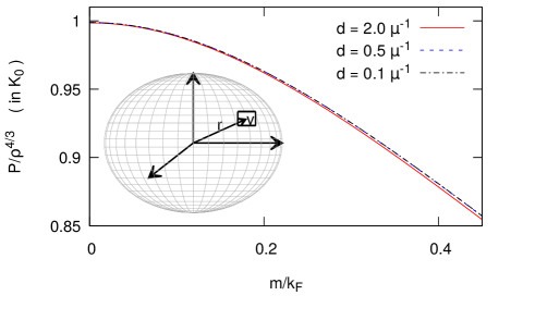
Figure 1: (i) A finite box of volume $V$ at the given coordinate $r$ within a spherical star (inset figure). (ii) Different values of $d$ lead to same polytropic constant in the ultra-relativistic limit of the general equation of state.

Within a spherically symmetric white dwarf, the pressure and mass density vary radially. However, to employ the techniques of finite temperature quantum field theory we have to consider a spatial region which is in thermal equilibrium at a given temperature $T$ along with uniform pressure and mass density. Therefore, around a given radial coordinate, we consider a finite spatial box which is sufficiently small so that the pressure and energy density can be treated to be uniform and yet sufficiently large to contain enough degrees of freedom to achieve required thermodynamical equilibrium (see FIG.1). The partition function that describes the degrees of freedom within the box, can be expressed as $\mathcal{Z}=Tr[e^{-\beta(\hat{H}-\mu\hat{Q})}]$, where $\beta=1/k_{B}T$ with $k_{B}$ being the Boltzmann constant, $\mu$ is the chemical potential and $Q$ refers to the conserved charge of the system. The Hamiltonian operator $\hat{H}$ represents the matter fields.

Matter fields.– The degenerate electrons within the box along with the spacetime metric $\eta_{\mu\nu}=diag(-1,1,1,1)$, are represented by the Dirac spinor field $\psi$ with the free-field action

$$S_{\psi}=\int d^{4}x\mathcal{L}_{\psi}=-\int d^{4}x~{}\bar{\psi}[i\gamma^{\mu}\partial_{\mu}+m]\psi~{},$$ (2)

where the Dirac matrices $\gamma^{\mu}$ satisfies the anti-commutation relation $\{\gamma^{\mu},\gamma^{\nu}\}=-2\eta^{\mu\nu}\mathbb{I}$. The minus sign in front of $\eta^{\mu\nu}$ is chosen such that the Dirac matrices satisfies the usual relations $(\gamma^{0})^{2}=\mathbb{I}$ and $(\gamma^{k})^{2}=-\mathbb{I}$ where $k=1,2,3$. The electromagnetic interaction between the electrons are mediated by the gauge fields $A_{\mu}$ and described by the action

$$S_{I}^{-}=\int d^{4}x\mathcal{L}_{I}^{-}=\int d^{4}x~{}\bar{\psi}[e~{}\gamma^{\mu}A_{\mu}]\psi~{},$$ (3)

where $e$ is the electromagnetic coupling constant. On the other hand the free-field dynamics of $A_{\mu}$ is governed by the Maxwell action

$$S_{A}=\int d^{4}x\mathcal{L}_{A}=\int d^{4}x~{}\left[-\frac{1}{4}F_{\mu\nu}F^{\mu\nu}\right]~{},$$ (4)

where the field strength $F_{\mu\nu}=\partial_{\mu}A_{\nu}-\partial_{\nu}A_{\mu}$. The actions (2,3,4) together form the total action, say $S_{QED}$, used in the quantum electrodynamics.

The conserved 4-current corresponding to the action (2) is given by $j^{\mu}=\bar{\psi}\gamma^{\mu}\psi$ which represents the contribution from the electrons. Similarly, we may consider a background 4-current, say $J^{\mu}$, to represent the contribution from the positively charged nuclei which are usually bosonic degrees of freedom. Therefore, to describe the interaction between the electrons and the positively charged nuclei, here we consider a Lorentz invariant current-current interaction term as follows

$$S_{I}^{+}=\int d^{4}x\mathcal{L}_{I}^{+}=\int d^{4}x~{}[-Ze^{2}d^{2}~{}J_{\mu}\bar{\psi}\gamma^{\mu}\psi]~{}.$$ (5)

In Eq. (5), the coupling constant contains the term $-Ze^{2}$ which signifies the strength of the attractive interaction between an electron and a positively charged nucleus with atomic number $Z$. The parameter $d$ which has the dimension of length, is introduced to make the action (5) dimensionless and it represents the interaction scale associated with the current-current interaction between the electrons and the nuclei. Therefore, the total action that describes the dynamics of the degenerate electrons within a white dwarf is given by

$$S=S_{QED}+S_{I}^{+}=S_{\psi}+S_{A}+S_{I}=:\int d^{4}x\mathcal{L}~{},$$ (6)

where $S_{I}=S_{I}^{-}+S_{I}^{+}$. Inclusion of the additional interaction term (5) preserves the symmetry of the action $S_{QED}$. In other words, apart from being Lorentz invariant, the total action (6) is also invariant under local U(1) gauge transformations $\psi(x)\rightarrow e^{i\alpha(x)}\psi(x)$ and $A_{\mu}\rightarrow A_{\mu}-\frac{1}{e}\partial_{\mu}\alpha(x)$ with $\alpha(x)$ being an arbitrary function. Given the coupling constant $e$ is small, we can study the interacting theory by perturbative techniques of finite temperature quantum field theory.

Partition function.– To evaluate the partition function here we follow the path integral approach. In order to avoid over-counting of gauge degrees of freedom of $A_{\mu}$, it is convenient to introduce the Faddeev-Popov ghost fields $C$ and $\bar{C}$ along with its action $S_{C}=\int d^{4}x\mathcal{L}_{C}=\int d^{4}x\partial^{\mu}\bar{C}\partial_{\mu}C$ Weinberg (1995); Nair (2005). These Grassmann-valued fields effectively cancel the contributions from two gauge degrees of freedom. Therefore, the thermal partition function containing contributions from all the physical fields can be written as

$$\mathcal{Z}=\int\mathcal{D}\bar{\psi}\mathcal{D}\psi\mathcal{D}A_{\mu}\mathcal{D}\bar{C}~{}\mathcal{D}C~{}e^{-S^{\beta}}~{},$$ (7)

where Euclidean action $S^{\beta}=\int_{0}^{\beta}d\tau\int d^{3}\mathbf{x}~{}[\mathcal{L}+\mu\psi^{\dagger}\psi]_{|t=i\tau}=:S_{\psi}^{\beta}+(S_{A}^{\beta}+S_{C}^{\beta})+S_{I}^{\beta}$ with $S_{\psi}^{\beta}=\int_{0}^{\beta}d\tau\int d^{3}\mathbf{x}[\mathcal{L}_{\psi}+\mu\psi^{\dagger}\psi]_{|t=i\tau}$. We can express the total partition function using perturbative methods as $\ln\mathcal{Z}=\ln\mathcal{Z}_{\psi}+\ln\mathcal{Z}_{A}+\ln\mathcal{Z}_{I}$.

In the functional integral (7) both fields $A_{\mu}(x)$ and $C(x)$ are subject to the periodic boundary conditions $A_{\mu}(\tau,\mathbf{x})=A_{\mu}(\tau+\beta,\mathbf{x})$ and $C(\tau,\mathbf{x})=C(\tau+\beta,\mathbf{x})$ whereas the spinor field is subject to the anti-periodic boundary condition $\psi(\tau,\mathbf{x})=-\psi(\tau+\beta,\mathbf{x})$. The spinor field can be Fourier transformed as

$$\psi(\tau,\mathbf{x})=\frac{1}{\sqrt{V}}\sum_{n,\mathrm{k}}~{}e^{i(\omega_{n}\tau+\mathrm{k}\cdot\mathbf{x})}\tilde{\psi}(n,\mathrm{k})~{},$$ (8)

where $V$ is the spatial volume of the box. The spinor field has mass dimension $3/2$ in natural units. So the Fourier modes $\tilde{\psi}(n,\mathrm{k})$ are dimensionless. Further, the anti-periodic boundary condition implies that the Matsubara frequencies $\omega_{n}=(2n+1)\pi~{}\beta^{-1}$ where $n$ is an integer. Using Eq. (8), the Euclidean action for the spinor field can be expressed as

$$S_{\psi}^{\beta}=\sum_{n,\mathrm{k}}~{}\bar{\tilde{\psi}}~{}\beta\left[\not{p}-m\right]\tilde{\psi}~{},$$ (9)

where $p_{\mu}=(p_{0},\vec{p})=(-i\omega_{n}+\mu,\mathrm{k})$ and $\not{p}=\gamma^{\mu}p_{\mu}$. The Eq. (9) leads to momentum space thermal propagator for the free spinor field as $\mathcal{G}^{0}(\omega_{n},\mathrm{k})=1/(\not{p}-m)=-(\not{p}+m)/(p^{2}+m^{2})$ where $p^{2}=p^{\mu}p_{\mu}$. If one carries out the summation over $n$ by disregarding the formally divergent terms and the contribution from the anti-particles then fermionic part of the partition function becomes $\ln\mathcal{Z}_{\psi}=2\sum_{\mathrm{k}}\left[\ln\left(1+e^{-\beta(\omega-\mu)}\right)\right]$ where $\omega^{2}=(\mathrm{k}^{2}+m^{2})$. The factor of 2 here denotes the spin-degeneracy of the electrons. To carry out the summation over $\mathrm{k}$, one may convert it to an integral as $\sum_{\mathrm{k}}\to V\int\frac{d^{3}\mathrm{k}}{(2\pi)^{3}}$. The Fermi momentum $k_{F}\equiv\sqrt{\mu^{2}-m^{2}}$ implies that for typical white dwarfs $\beta\mu\gg 1$. This strong inequality in turns allows the approximation $(e^{\beta(\omega-\mu)}+1)^{-1}\simeq\Theta(\mu-\omega)-\mathrm{sgn}(\mu-\omega)e^{-\beta|\mu-\omega|}$ where $\Theta(\mu-\omega)$ is the Theta function and $\mathrm{sgn}(x)$ is the signum function. The evaluation of the integral Joseph I. Kapusta (2006); Hossain and Mandal (2019) then leads to

$$\ln\mathcal{Z}_{\psi}=\frac{\beta V}{24\pi^{2}}\left[2\mu k_{F}^{3}-3m^{2}\bar{k}_{F}^{2}+\frac{48\mu k_{F}}{\beta^{2}}\right]~{},$$ (10)

where $\bar{k}_{F}^{2}\equiv\mu k_{F}-m^{2}\ln\left((\mu+k_{F})/m\right)$. The physical contribution from the gauge fields can be written as $\ln\mathcal{Z}_{A}=\ln(\int\mathcal{D}A_{\mu}\mathcal{D}\bar{C}~{}\mathcal{D}C~{}e^{-(S_{A}^{\beta}+S_{C}^{\beta})})=\tfrac{1}{45}V\pi^{2}\beta^{-3}$ which makes negligible contribution to the white dwarf equation of state and henceforth neglected.

The leading order contribution from the interaction terms can be expressed as $\ln\mathcal{Z}_{I}=\tfrac{1}{2}\langle(S_{-}^{\beta})^{2}\rangle-\langle{S_{+}^{\beta}}\rangle$ where $\langle.\rangle$ denotes ensemble average. The contribution due to the self-interaction of the electrons is Joseph I. Kapusta (2006); Hossain and Mandal (2019)

$$\langle(S_{-}^{\beta})^{2}\rangle=\frac{\beta Ve^{2}}{4\pi^{2}}\left(\frac{\bar{k}_{F}^{4}}{4\pi^{2}}+\frac{\bar{k}_{F}^{2}}{3\beta^{2}}\right)~{}.$$ (11)

Using the Eq. (5), we can express the contribution due to the interaction between the electrons and positively charged nuclei as

$$\langle S_{+}^{\beta}\rangle=-Ze^{2}d^{2}\int_{0}^{\beta}d\tau\int d^{3}\mathbf{x}J_{\mu}(\tau,\mathbf{x})\langle\overline{\psi}(\tau,\mathbf{x})\gamma^{\mu}\psi(\tau,\mathbf{x})\rangle~{}.$$ (12)

The Fourier space thermal propagator $\mathcal{G}(\omega_{n},\mathrm{k})=\int_{0}^{\beta}d\tau\int d^{3}\mathbf{x}~{}e^{-i(\omega_{n}\tau+\mathrm{k}\cdot\mathbf{x})}\langle\psi(\tau_{1},\mathbf{x}_{1})\overline{\psi}(\tau_{2},\mathbf{x}_{2})\rangle$ along with $\tau=\tau_{1}-\tau_{2}$, $\mathbf{x}=\mathbf{x}_{1}-\mathbf{x}_{2}$, leads the Eq. (12) to become

$$\langle S_{+}^{\beta}\rangle=-Ze^{2}d^{2}\tilde{J}_{\mu}(\beta)\sum_{n,\mathrm{k}}~{}\mathrm{Tr}\left[\gamma^{\mu}\mathcal{G}(\omega_{n},\mathrm{k})\right]~{},$$ (13)

where the trace is over the Dirac indices and the average background 4-current density is $\tilde{J}_{\mu}(\beta)=(\beta V)^{-1}\int_{0}^{\beta}d\tau\int d^{3}\mathbf{x}~{}J_{\mu}(\tau,\mathbf{x})$. We assume background 3-current density $\tilde{J}^{k}$ of the heavier nuclei is vanishing and identify corresponding charge density as $n_{+}\equiv\tilde{J}^{0}=-\tilde{J}_{0}$. The Eq. (13) then simplifies to

$$\langle S_{+}^{\beta}\rangle=\frac{\beta VZe^{2}d^{2}k_{F}^{3}n_{+}}{3\pi^{2}}~{}.$$ (14)

Overall the system is electrically neutral. So the number density of positively charged nuclei must satisfy $Zn_{+}=n_{e}$ where $n_{e}$ is the number density of the electrons. So the contribution to the partition function from the combined interaction becomes

$$\ln\mathcal{Z}_{I}=\frac{\beta Ve^{2}}{96\pi^{4}}\left(3\bar{k}_{F}^{4}-32\pi^{2}dn_{e}k_{F}^{3}\right)~{},$$ (15)

where we have ignored finite temperature corrections inside the parenthesis as the $(\beta k_{F})^{-1}$ and coupling constant $e$ both are small.

Equation of state.– In order to understand the Chandrasekhar mass limit it is sufficient to evaluate the equation of state in its ultra-relativistic limit i.e. when $k_{F}\gg m$, $\bar{k}_{F}\simeq k_{F}$ and $\mu\simeq k_{F}$ (see Hossain and Mandal (2019) for general equation of state). As $(\beta k_{F})^{-2}\sim 10^{-9}$ for typical white dwarfs then the Eqs. (10, 15) imply that the finite temperature corrections are much smaller compared to the corrections arising due to the fine-structure constant $\alpha\equiv e^{2}/4\pi\simeq 1/137$. Therefore, in the ultra-relativistic limit, the total partition function including the leading order $\alpha$ corrections but ignoring the finite temperature corrections, can be expressed as

$$\ln\mathcal{Z}=\frac{\beta V}{12\pi^{2}}\left[k_{F}^{4}+\frac{\alpha}{2\pi}\left(3k_{F}^{4}-32\pi^{2}d^{2}n_{e}k_{F}^{3}\right)\right]~{}.$$ (16)

The number density of the degenerate electrons can be computed as $n_{e}\equiv\langle N\rangle/V=(\beta V)^{-1}(\partial\ln\mathcal{Z}/\partial\mu)$. Given total partition function (15) itself depends on the electron number density, it leads to an algebraic equation for $n_{e}$ as given below

$$n_{e}=\frac{k_{F}^{3}}{3\pi^{2}}\left[1+\frac{3\alpha}{2\pi}\left(1-8\pi^{2}d^{2}n_{e}k_{F}^{-1}\right)\right]~{}.$$ (17)

The Eq. (17) can be solved to express the corresponding mass density $\rho\equiv\mu_{e}m_{u}n_{e}$ as

$$\rho=\frac{\mu_{e}m_{u}k_{F}^{3}}{3\pi^{2}}\left[1+\frac{\alpha}{2\pi}\left(3-2d_{+}^{2}\right)\right]~{},$$ (18)

where $d_{+}\equiv 2d\mu$ and $m_{u}$ is the atomic mass unit. The chemical potential $\mu$ in the partition function provides a natural scale to construct the dimensionless parameter $d_{+}$ which characterizes the electron-nuclei interaction. The parameter $\mu_{e}\equiv(A/Z)$ with $A$ being the atomic mass number, is defined so that $\mu_{e}m_{u}$ specifies ‘the average mass per electron’.

In a grand canonical ensemble, we may read off the degeneracy pressure of the electrons as $P=(\beta V)^{-1}\ln\mathcal{Z}$ which leads to

$$P=\frac{k_{F}^{4}}{12\pi^{2}}\left[1+\frac{\alpha}{6\pi}\left(9-8d_{+}^{2}\right)\right]~{}.$$ (19)

By Combining the Eqs. (18) and (19), it is straightforward to write down a polytropic equation of state $P=\mathrm{K}\rho^{4/3}$ with

$$\mathrm{K}=\frac{(3\pi^{2})^{1/3}(1-\alpha/2\pi)}{4(\mu_{e}m_{u})^{4/3}}=\mathrm{K}_{0}(1-\alpha/2\pi)~{},$$ (20)

where $K_{0}$ is the polytropic constant without $\alpha$ corrections. Clearly, the ratio $P/\rho^{4/3}$ for the degenerate matter becomes independent of the interaction between the electrons and the nuclei in the ultra-relativistic limit $k_{F}\gg m$ (see FIG.1 for its dependence on $m/K_{F}$). However, in the non-relativistic limit, this interaction does contribute Hossain and Mandal (2019).

Chandrasekhar mass limit.– In order to find the Chandrasekhar mass limit, it is convenient to express the pressure as $P=\mathrm{K}\rho^{1+1/n}$ where $n=3$. Subsequently, one defines a dimensionless function $\theta(r)$ so that the mass density can be written as $\rho(r)=\rho_{c}\theta^{n}$. The identification of $\rho_{c}$ with central density implies $\theta(0)=1$. The second boundary condition $\theta^{\prime}(0)=0$ follows from the condition $dP/dr=0$ at $r=0$. Further, one defines a dimensionless variable $\xi=r/a$ where $a^{2}=(\mathrm{K}/\pi G)\rho_{c}^{-2/3}$. The hydro-static equilibrium condition then leads to the Lane-Emden equation $\xi^{-2}\frac{d}{d\xi}\left(\xi^{2}\frac{d\theta}{d\xi}\right)=-\theta^{n}$. The Chandrasekhar mass limit is then defined as $M_{ch}=\int_{0}^{R}4\pi r^{\prime 2}\rho(r^{\prime})dr^{\prime}$ where $R$ is the radius of the white dwarf. As $n=3$ here, the Chandrasekhar mass limit can be explicitly expressed as $M_{ch}=(4/\sqrt{\pi})\left(\mathrm{K}/G\right)^{3/2}|\xi_{0}^{2}~{}\theta^{\prime}(\xi_{0})|$ where at the boundary $\xi_{0}=R/a$ the mass density vanishes i.e. $\theta(\xi_{0})=0$. The Lane-Emden equation can be solved numerically to find $|\xi_{0}^{2}~{}\theta^{\prime}(\xi_{0})|\simeq 2.02$. Therefore, including the leading order effect of the fine structure constant, the Chandrasekhar mass limit becomes

$$M_{ch}=M_{ch}^{0}\left(1-\frac{3\alpha}{4\pi}\right)~{},$$ (21)

where $M_{ch}^{0}$ denotes the Chandrasekhar mass limit without $\alpha$ corrections. In other words, the effects of fine-structure constant reduces the Chandrasekhar mass limit by a universal factor which in the leading order does not depend on the atomic number $Z$ of the positively charge nuclei of the degenerate matter, unlike the results obtained in Hamada and Salpeter (1961); Nauenberg (1972).

Using the value of the fine structure constant $\alpha\simeq 1/137$, we observe that the Chandrasekhar mass limit is reduced by $0.17\%$ and similar order corrections are present in the corresponding equation of state. The future detection of low-frequency gravitational waves from the extreme mass-ratio merger of a black whole with a white dwarf could determine the equation of state of the degenerate matter within the white dwarf with an accuracy reaching up to $0.1\%$ Han and Fan (2018). Therefore, the effects of fine-structure constant corrections as studied here would be within the detection threshold of such gravitational wave detectors in the future.

Acknowledgments.– SM thanks CSIR, India for supporting this work through a doctoral fellowship.

References

- Abbott et al. (2016) B. P. Abbott et al. (LIGO Scientific, Virgo), Phys. Rev. Lett. 116, 061102 (2016), eprint arXiv:1602.03837.
- Abbott et al. (2017) B. Abbott et al. (LIGO Scientific, Virgo), Phys. Rev. Lett. 119, 161101 (2017), eprint arXiv:1710.05832.
- Annala et al. (2018) E. Annala, T. Gorda, A. Kurkela, and A. Vuorinen, Phys. Rev. Lett. 120, 172703 (2018), eprint 1711.02644.
- Abbott et al. (2018) B. P. Abbott et al. (LIGO Scientific, Virgo), Phys. Rev. Lett. 121, 161101 (2018), eprint arXiv:1805.11581.
- Nandi et al. (2018) R. Nandi, P. Char, and S. Pal (2018), eprint arXiv:1809.07108.
- Amaro-Seoane et al. (2012) P. Amaro-Seoane, S. Aoudia, S. Babak, P. Binetruy, E. Berti, A. Bohe, C. Caprini, M. Colpi, N. J. Cornish, K. Danzmann, et al., Classical and Quantum Gravity 29, 124016 (2012).
- Han and Fan (2018) W.-B. Han and X.-L. Fan, Astrophys. J. 856, 82 (2018), eprint arXiv:1711.08628.
- Holberg et al. (2012) J. B. Holberg, T. D. Oswalt, and M. A. Barstow, Astron. J. 143, 68 (2012), eprint arXiv:1201.3822.
- Tremblay et al. (2017) P.-E. Tremblay, N. Gentile-Fusillo, R. Raddi, S. Jordan, C. Besson, B. T. Gänsicke, S. G. Parsons, D. Koester, T. Marsh, R. Bohlin, et al., Monthly Notices of the Royal Astronomical Society 465, 2849 (2017), eprint arXiv:1611.00629.
- Magano et al. (2017) D. M. N. Magano, J. M. A. Vilas Boas, and C. J. A. P. Martins, Phys. Rev. D96, 083012 (2017), eprint arXiv:1710.05828.
- Chandrasekhar (1931) S. Chandrasekhar, The Astrophysical Journal 74, 81 (1931).
- Chandrasekhar (1935) S. Chandrasekhar, Monthly Notices of the Royal Astronomical Society 95, 207 (1935).
- Kothari (1938) D. Kothari, Proceedings of the Royal Society of London. Series A, Mathematical and Physical Sciences pp. 486–500 (1938).
- Auluck and Mathur (1959) F. Auluck and V. Mathur, Zeitschrift fur Astrophysik 48, 28 (1959).
- Salpeter (1961) E. E. Salpeter, The Astrophysical Journal 134, 669 (1961).
- Rotondo et al. (2011) M. Rotondo, J. A. Rueda, R. Ruffini, and S.-S. Xue, Phys. Rev. D 84, 084007 (2011).
- Hamada and Salpeter (1961) T. Hamada and E. Salpeter, The Astrophysical Journal 134, 683 (1961).
- Nauenberg (1972) M. Nauenberg, The Astrophysical Journal 175, 417 (1972).
- Matsubara (1955) T. Matsubara, Progress of theoretical physics 14, 351 (1955).
- Akhiezer and Peletminskii (1960) I. Akhiezer and S. Peletminskii, Zh. Eksp. Teor. Fiz. 11, 1316 (1960).
- Freedman and McLerran (1977) B. A. Freedman and L. D. McLerran, Phys. Rev. D 16, 1147 (1977).
- Joyce et al. (2018) S. R. G. Joyce, M. A. Barstow, J. B. Holberg, H. E. Bond, S. L. Casewell, and M. R. Burleigh, Monthly Notices of the Royal Astronomical Society 481, 2361 (2018), eprint arXiv:1809.01240.
- Weinberg (1995) S. Weinberg, Quantum theory of fields. Foundations, vol. Volume 1 (Cambridge University Press, 1995), 1st ed.
- Nair (2005) V. P. Nair, Quantum Field Theory: A Modern Perspective, Graduate Texts in Contemporary Physics (Springer, 2005), 1st ed.
- Joseph I. Kapusta (2006) C. G. Joseph I. Kapusta, Finite-Temperature Field Theory: Principles and Applications, Cambridge Monographs on Mathematical Physics (Cambridge University Press, 2006), 2nd ed.
- Hossain and Mandal (2019) G. M. Hossain and S. Mandal (2019), eprint arXiv:1904.09174.