Non-local Attention Optimized Deep Image Compression

Abstract

This paper proposes a novel Non-Local Attention Optimized Deep Image Compression (NLAIC) framework, which is built on top of the popular variational auto-encoder (VAE) structure. Our NLAIC framework embeds non-local operations in the encoders and decoders for both image and latent feature probability information (known as hyperprior) to capture both local and global correlations, and apply attention mechanism to generate masks that are used to weigh the features for the image and hyperprior, which implicitly adapt bit allocation for different features based on their importance. Furthermore, both hyperpriors and spatial-channel neighbors of the latent features are used to improve entropy coding. The proposed model outperforms the existing methods on Kodak dataset, including learned (e.g., Balle2019 [18], Balle2018 [5]) and conventional (e.g., BPG, JPEG2000, JPEG) image compression methods, for both PSNR and MS-SSIM distortion metrics.

1 Introduction

Most recently proposed machine learning based image compression algorithms [5, 20, 17] leverage the autoencoder structure, which transforms raw pixels into compressible latent features via stacked convolutional neural networks (CNNs). These latent features are entropy coded subsequently by exploiting the statistical redundancy. Recent prior works have revealed that compression efficiency can be improved when exploring the conditional probabilities via the contexts of spatial neighbors and hyperpriors [17, 11, 5]. Typically, rate-distortion optimization [21] is fulfilled by minimizing Lagrangian cost $J$ = $R$ + $\lambda$$D$, when performing the end-to-end training. Here, $R$ is referred to as entropy rate, and $D$ is the distortion measured by either mean squared error (MSE) or multiscale structural similarity (MS-SSIM) [25].

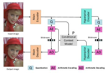
Figure 1: Proposed NLAIC framework using a variational autoencoder structure with embedded non-local attention optimization in the main and hyperprior encoders and decoders.

However, existing methods still present several limitations. For example, most of the operations, such as stacked convolutions, are performed locally with limited receptive field, even with pyramidal decomposition. Furthermore, latent features are treated with equal importance in either spatial or channel dimension in most works, without considering the diverse visual sensitivities to various contents (such as texture and edge). Thus, attempts have been made in [11, 17] to exploit importance maps on top of latent feature vectors for adaptive bit allocation. But these methods require the extra explicit signaling overhead to carry the importance maps.

In this paper, we introduce non-local operation blocks proposed in [24] into the variational autoencoder (VAE) structure to capture both local and global correlations among pixels, and generate the attention masks which help to yield more compact distributions of latent features and hyperpriors.Different from those existing methods in [11, 17], we use non-local processing to generate attention masks at different layers (not only for quantized features), to allocate the bits intelligently through the end-to-end training. We also improve the context modeling of the entropy engine for better latent feature compression, by using a masked 3D CNN (i.e., 5$\times$5$\times$5) on the latent features to generate the conditional statistics of the latent features.

Two different model implementations are provided, one is the “NLAIC joint” , which uses both hyperpriors and spatial-channel neighbors in the latent features for context modeling, and the other is the “NLAIC baseline” with contexts only from hyperpriors. Our joint model outperforms all existing learned and traditional image compression methods, in terms of the rate distortion efficiency for the distortion measured by both MS-SSIM and PSNR.

To further verify the efficiency of our framework, we also conduct ablation studies to discuss model variants such as removing non-local operations and attention mechanisms layer by layer, as well as the visual comparison. These additional experiments provide further evidence of the superior performance of our proposed NLAIC framework over a broad dataset.

The main contributions of this paper are highlighted as follows:

• We are the first to introduce non-local operations into compression framework to capture both local and global correlations among the pixels in the original image and feature maps.

• We apply attention mechanism together with aforementioned non-local operations to generate implicit importance masks to guide the adaptive processing of latent features. These masks essentially allocate more bits to more important features that are critical for reducing the image distortion.

• We employ a one-layer masked 3D CNN to exploit the spatial and cross channel correlations in the latent features, the output of which is then concatenated with hyperpriors to estimate the conditional statistics of the latent features, enabling more efficient entropy coding.

Table 1: Detailed Parameter Settings in NLAIC as shown in Fig. 1: “Conv” denotes a convolution layer with kernel size and number of output channels. “s” is the stride (e.g.,s2 means a down/up-sampling with stride 2). NLAM represents the non-local attention modules. “$\times$3” means cascading 3 residual blocks (ResBlock).

Main Encoder	Main Decoder	Hyperprior Encoder	Hyperprior Decoder	Conditional Context Model
Conv: 5$\times$5$\times$192 s2	NLAM	ResBlock($\times$3): 3$\times$3$\times$192	NLAM	Masked: 5$\times$5$\times$5$\times$24 s1
ResBlock($\times$3): 3$\times$3$\times$192	Deconv: 5$\times$5$\times$192 s2	Conv: 5$\times$5$\times$192 s2	Deconv: 5$\times$5$\times$192 s2	Conv: 1$\times$1$\times$1$\times$48 s1
Conv: 5$\times$5$\times$192 s2	ResBlock($\times$3): 3$\times$3$\times$192	ResBlock($\times$3): 3$\times$3$\times$192	ResBlock($\times$3): 3$\times$3$\times$192	ReLU
NLAM	Deconv: 5$\times$5$\times$192 s2	Conv: 5$\times$5$\times$192 s2	Deconv: 5$\times$5$\times$192 s2	Conv: 1$\times$1$\times$1$\times$96 s1
Conv: 5$\times$5$\times$192 s2	NLAM	NLAM	ResBlock($\times$3): 3$\times$3$\times$192	ReLU
ResBlock($\times$3): 3$\times$3$\times$192	Deconv: 5$\times$5$\times$192 s2		Conv: 5$\times$5$\times$384 s1	Conv: 1$\times$1$\times$1$\times$2 s1
Conv: 5$\times$5$\times$192 s2	ResBlock($\times$3): 3$\times$3$\times$192
NLAM	Conv: 5$\times$5$\times$3 s2

2 Related Work

Non-local Operations. Most traditional filters (such as Gaussian and mean) process the data locally, by using a weighted average of spatially neighboring pixels. It usually produces over-smoothed reconstructions. Classical non-local methods for image restoration problems (e.g., low-rank modeling [9], joint sparsity [16] and non-local means [7]) have shown their superior efficiency for quality improvement by exploiting non-local correlations. Recently, non-local operations haven been included into the deep neural networks (DNN) for video classification [24], image restoration (e.g., denoising, artifacts removal and super-resolution) [13, 27], etc, with significant performance improvement reported. It is also worth to point out that non-local operations have been applied in other scenarios, such as intra block copy in screen content extension of the High-Efficiency Video Coding (HEVC) [26].

Self Attention. Self-attention mechanism is widely used in deep learning based natural language processing (NLP) [15, 8, 23]. It can be described as a mapping strategy which queries a set of key-value pairs to an output. For example, Vaswani et. al [23] have proposed multi-headed attention methods which are extensively used for machine translation. For those low-level vision tasks [27, 11, 17], self-attention mechanism makes generated features with spatial adaptive activation and enables adaptive information allocation with the emphasis on more challenging areas (i.e., rich textures, saliency, etc).

In image compression, quantized attention masks are commonly used for adaptive bit allocation, e.g., Li et. al [11] uses 3 layers of local convolutions and Mentzer et. al [17] selects one of the quantized features. Unfortunately, these methods require the extra explicit signaling overhead. Our model adopts attention mechanism that is close to [11, 17] but applies multiple layers of non-local as well as convolutional operations to automatically generate attention masks from the input image. The attention masks are applied to the temporary latent features directly to generate the final latent features to be coded. Thus, there is no need to use extra bits to code the masks.

Image Compression Architectures. DNN based image compression generally relies on well-known autoencoders. Its back propagation scheme requires all the steps differentiable in an end-to-end manner. Several methods (e.g., adding uniform noise [4], replacing the direct derivative with the derivative of the expectation [22] and soft-to-hard quantization [3]) are developed to approximate the non-differentiable quantization process. On the other hand, entropy rate modeling of quantized latent features is another critical issue for learned image compression. PixelCNNs [19] and VAE are commonly used for entropy estimation following the Bayesian generative rules. Recently, conditional probability estimates based on autoregressive neighbors of the latent feature maps and hyperpriors jointly has shown significant improvement in entropy coding.

3 Non-Local Attention Implementation

3.1 General Framework

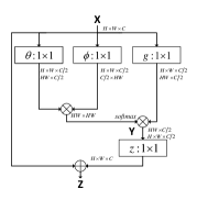
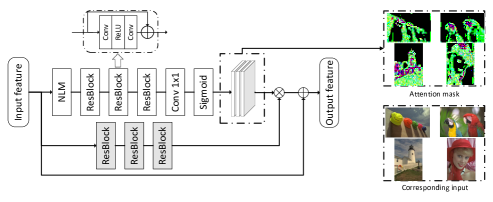
Figure 2: (a) Non-local module (NLM). $H\times{W}\times{C}$ denotes the size of fearure maps with height $H$, width $W$ and channel $C$. $\oplus$ is the add operation and $\otimes$ is the matrix multiplication. (b) Non-local attention module (NLAM). The main branch consists of 3 residual blocks.The mask branch combines non-local modules with residual blocks for attention mask generation. The details of residual blocks are shown in the dash frame.

Fig. 1 illustrates our NLAIC framework. It is built on a variational autoencoder structure [5], with non-local attention modules (NLAM) as basic units in both main and hyperprior encoder-decoder pairs (i.e., ${\mathbb{E}}_{M}$, ${\mathbb{D}}_{M}$, ${\mathbb{E}}_{h}$ and ${\mathbb{D}}_{h}$). ${\mathbb{E}}_{M}$ with quantization $Q$ are used to generate latent quantized features and ${\mathbb{E}}_{D}$ decodes the features into the reconstructed image. ${\mathbb{E}}_{h}$ and ${\mathbb{D}}_{h}$ generate much smaller side information as hyperpriors. The hyperpriors as well as autoregressive neighbors of the latent features are then processed through the conditional context model ${\mathbb{P}}$ to generate the conditional probability estimates for entropy coding of the latent quantized features.

Table 1 details the network structures and associated parameters of five different components in the proposed NLAIC framework. The NLAM module is shown in Fig. 2, and explained in Sections 3.2 and 3.3.

3.2 Non-local Module

Our NLAM adopts the non-local network proposed in  [24] as a basic block, as shown in Fig. 2. As shown in Fig. 2, the non-local module (NLM) computes the output at pixel $i$, $Y_{i}$, using a weighted average of the transformed feature values at pixel $j$, $X_{j}$, as below:

$$Y_{i}=\frac{1}{C(X)}{\sum_{{\forall}j}}f(X_{i},X_{j})g(X_{j}),$$ (1)

where $i$ is the location index of output vector $Y$ and $j$ represents the index that enumerates all accessible positions of input $X$. $X$ and $Y$ share the same size. The function $f(\cdot)$ computes the correlations between $X_{i}$ and $X_{j}$, and $g(\cdot)$ computes the representation of the input at the position $j$. $C(X)$ is a normalizing factor to generate the final response which is set as $C(X)=\sum_{\forall j}f(X_{i},X_{j})$. Note that a variety of function forms of $f(\cdot)$ have been already discussed in [24]. Thus in this work, we directly use the embedded Gaussian function for $f(\cdot)$, i.e.,

$$f(X_{i},X_{j})=e^{\theta(X_{i}^{T})\phi(X_{j})}.$$ (2)

Here, $\theta(X_{i})=W_{\theta}{X_{i}}$ and $\phi(X_{j})=W_{\phi}{X_{j}}$, where $W_{\theta}$ and $W_{\phi}$ denote the cross-channel transform using 1$\times$1 convolution in our framework. The weights $f(X_{i},X_{j})$ are further modified by a softmax operation. The operation defined in Eq. (1) can be written in matrix form [24] as:

$$Y={\tt softmax}({X}^{T}W_{\theta}^{T}W_{\phi}{X})g(X).$$ (3)

In addition, residual connection can be applied for better convergence as suggested in [24], as shown in Fig. 2, i.e.,

$$Z_{i}=W_{z}Y_{i}+X_{i},$$ (4)

where $W_{z}$ is also a linear 1$\times$1 convolution across all channels, and $Z_{i}$ is the final output vector.

3.3 Non-local Attention Module

Importance map has been adopted in [11, 17] to adaptively allocate information to quantized latent features. For instance, we can give more bits to textured area but less bits to elsewhere, resulting in better visual quality at the similar bit rate. Such adaptive allocation can be implemented by using an explicit mask, which must be specified with additional bits. As aforementioned, existing mask generation methods in [11, 17] are too simple to handle areas with more complex content characteristics.

Inspired by [27], we propose to use a cascade of a non-local module and regular convolutional layers to generate the attention masks, as shown in Fig. 2. The NLAM consists of two branches. The main branch uses conventional stacked networks to generate features and the mask branch applies the NLM with three residual blocks [10], one 1$\times$1 convolution and sigmoid activation to produce a joint spatial-channel attention mask $M$, i.e.,

$$M={\tt sigmoid}(F_{\rm NLM}(X)),$$ (5)

where $M$ denotes the attention mask and $X$ is the input features. $F_{\rm NLM}(\cdot)$ represents the operations of using NLM with subsequent three residual blocks and 1$\times$1 convolution which are shown in Fig. 2. This attention mask $M$, having its element $0<M_{k}<1,M_{k}\in{\mathbb{R}}$, is element-wise multiplied with feature maps from the main branch to perform adaptive processing. Finally a residual connection is added for faster convergence.

We avoid any batch normalization (BN) layers and only use one ReLU in our residual blocks, justified through our experimental observations.

Note that in existing learned image compression methods, particularly for those with superior performance [4, 5, 18, 14], GDN activation has proven its better efficiency compared with ReLU, tanh, sigmoid, leakyReLU, etc. This may be due to the fact that GDN captures the global information across all feature channels at the same pixel location. However, we just use the simple ReLU function, and rely on our proposed NLAM to capture both the local and global correlations. We also find through experiments that inserting two pairs of two layers of NLAM for the main encoder-decoder, and one layer of NLAM in the hyperprior encoder-decoder, provides the best performance. As will be shown in subsequent Section 4, our NLAIC has demonstrated the state-of-the-art coding efficiency.

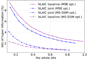
Figure 3: Illustration of percentage of $\hat{z}$ in the entire bitstream. For the case that model is optimized using MSE loss, $\hat{z}$ occupies less percentage for joint model than the baseline; But the outcome is reversed for the case that model is tuned with MS-SSIM loss. The percentage of $\hat{z}$ for MSE loss optimized method is noticeably higher than the scenario using MS-SSIM loss.

3.4 Entropy Rate Modeling

Previous sections present our novel NLAM scheme to transform the input pixels into more compact latent features. This section details the entropy rate modeling part that is critical for the overall rate-distortion efficiency.

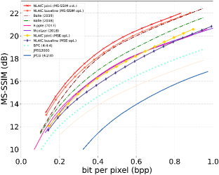
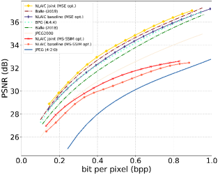
Figure 4: Illustration of the rate-distortion performance on Kodak. (a) distortion is measured by MS-SSIM (dB). Here we use $-10\log_{10}(1-d)$ to represent raw MS-SSIM ($d$) in dB scale. (b) PSNR is used for distortion measurement.

3.4.1 Context Modeling Using Hyperpriors

Similar as [5], a non-parametric, fully factorized density model is used for hyperpriors $\hat{z}$, which is described as:

$$p_{\hat{z}|\psi}(\hat{z}|\psi)={\prod_{i}}(p_{z_{i}|\psi^{(i)}}(\psi^{(i)})*\mathcal{U}(-\frac{1}{2},\frac{1}{2}))(\hat{z}_{i}),$$ (6)

where $\psi^{(i)}$ represents the parameters of each univariate distribution $p_{\hat{z}|\psi^{(i)}}$.

For quantized latent features $\hat{y}$, each element $\hat{y}_{i}$ can be modeled as a conditional Gaussian distribution as:

$$p_{\hat{y}|\hat{z}}(\hat{y}|\hat{z})={\prod_{i}}(\mathcal{N}(\mu_{i},{\sigma_{i}}^{2})*\mathcal{U}(-\frac{1}{2},\frac{1}{2}))(\hat{y}_{i}),$$ (7)

where its $\mu_{i}$ and $\sigma_{i}$ are predicted using the distribution of $\hat{z}$. We evaluate the bits of $\hat{y}$ and $\hat{z}$ using:

$$R_{\hat{y}} =-{\sum\nolimits_{i}}{\log_{2}}(p_{\hat{y}_{i}|\hat{z}_{i}}(\hat{y}_{i}|\hat{z}_{i})),$$ (8)

$$R_{\hat{z}} =-{\sum\nolimits_{i}}{\log_{2}}(p_{\hat{z}_{i}|\psi^{(i)}}({\hat{z}_{i}}|\psi^{(i)})).$$ (9)

Usually, we take $\hat{z}$ as side information for estimating $\mu_{i}$ and $\sigma_{i}$ and $\hat{z}$ only occupies a very small fraction of bits, shown in Fig. 3.

3.4.2 Context Modeling Using Neighbors

PixelCNNs and PixelRNNs [19] have been proposed for effective modeling of probabilistic distribution of images using local neighbors in an autoregressive way. It is further extended for adaptive context modeling in compression framework with noticeable improvement. For example, Minnen et al. [18] have proposed to extract autoregressive information by a 2D 5$\times$5 masked convolution, which is combined with hyperpriors using stacked 1$\times$1 convolution, for probability estimation. It is the first deep-learning based method with better PSNR compared with the BPG444 at the same bit rate.

In our NLAIC, we use a one-layer 5$\times$5$\times$5 3D masked convolution to exploit the spatial and cross-channel correlation. For simplicity, a 3$\times$3$\times$3 example is shown in Fig. 5.

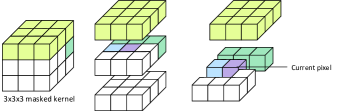
Figure 5: In 3$\times$3$\times$3 masked convolution, the current pixel (in purple) is predicted by the processed pixels (in yellow, green and blue) in a 3D space. The unprocessed pixels (in white) and the current pixel are masked with zeros.

Traditional 2D PixelCNNs need to search for a well structured channel order to exploit the conditional probability efficiently. Instead, our proposed 3D masked convolutions implicitly exploit correlation among adjacent channels. Compared to 2D masked CNN used in  [18], our 3D CNN approach significantly reduces the network parameters for the conditional context modeling. Leveraging the additional contexts from neighbors via an autoregressive fashion, we can obtain a better conditional Gaussian distribution to model the entropy as:

$$p_{\hat{y}}(\hat{y}_{i}|\hat{y}_{1},..., \hat{y}_{i-1},\hat{z})=$$

$${\prod_{i}}(\mathcal{N}(\mu_{i},{\sigma_{i}}^{2})*\mathcal{U}(-\frac{1}{2},\frac{1}{2}))(\hat{y}_{i}),$$ (10)

where $\hat{y}_{1},{\hat{y}}_{2},...,\hat{y}_{i-1}$ denote the causal (and possibly reconstructed) pixels prior to current pixel $\hat{y}_{i}$.

4 Experiments

4.1 Training

We use COCO [12] and CLIC [2] datasets to train our NLAIC framework. We randomly crop images into 192$\times$192$\times$3 patches for subsequent learning. Rate-distortion optimization (RDO) is applied to do end-to-end training at various bit rate, i.e.,

$$L={\lambda}{\cdot}d(\hat{x},x)+R_{y}+R_{z}.$$ (11)

$d(\cdot)$ is a distortion measurement between reconstructed image $\hat{x}$ and the original image $x$. Both negative MS-SSIM and MSE are used in our work as distortion loss for evaluation, which are marked as “MS-SSIM opt.” and “MSE opt.”, respectively. $R_{y}$ and $R_{z}$ represent the estimated bit rates of latent features and hyperpriors, respectively. Note that all components of our NLAIC are trained together. We set learning rates (LR) for ${\mathbb{E}}_{M}$, ${\mathbb{D}}_{M}$, ${\mathbb{E}}_{h}$, ${\mathbb{D}}_{h}$ and ${\mathbb{P}}$ at $3{\times}10^{-5}$ in the beginning. But for ${\mathbb{P}}$, its LR is clipped to $10^{-5}$ after 30 epochs. Batch size is set to 16 and the entire model is trained on 4-GPUs in parallel.

To understand the contribution of the context modeling using spatial-channel neighbors, we offer two different implementations: one is “NLAIC baseline” that only uses the hyperpriors to estimate the means and variances of the latent features (see Eq. (7)), while the other is “NLAIC joint” that uses both hyperpriors and previously coded pixels in the latent feature maps (see Eq. (10)). In this work, we first train the “NLAIC baseline” models. To train the “NLAIC joint” model, one way is fixing the main and hyperprior encoders and decoders in the baseline model, and updating only the conditional context model $\mathbb{P}$. Compared with the “NLAIC baseline”, such transfer learning based “NLAIC joint” provides 3% bit rate reduction at the same distortion. Alternatively, we could use the baseline models as the start point, and refine all the modules in the “NLAIC joint” system. In this way, “NLAIC joint” offers more than 9% bit rate reduction over the “NLAIC baseline” at the same quality. Thus, we choose the latter one for better performance.

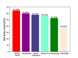
Figure 6: Coding efficiency comparison using JPEG as anchor. It shows our NLAIC achieves the best BD-Rate gains among all popular algorithms.

4.2 Performance Efficiency

We evaluate our NLAIC models by comparing the rate-distortion performance averaged on publicly available Kodak dataset. Fig. 4 shows the performance when distortion is measured by MS-SSIM and PSNR, respectively, that are widely used in image and video compression tasks. Here, PSNR represents the pixel-level distortion while MS-SSIM describes the structural similarity. MS-SSIM is reported to offer higher correlation with human perceptual inception, particularly at low bit rate [25]. As we can see, our NLAIC provides the state-of-the-art performance with noticeable performance margin compared with the existing leading methods, such as Ballé2019 [18] and Ballé2018 [5].

Specifically, as shown in Fig. 4 using MS-SSIM for both loss and final distortion measurement, “NLAIC baseline” outperforms the existing methods while the “NLAIC joint” presents even larger performance margin. For the case that uses MSE as loss and PSNR as distortion measurement, “NLAIC joint” still offers the best performance, as illustrated in Fig. 4. “NLAIC baseline” is slightly worse than the model in [18] that uses contexts from both hyperpriors and neighbors jointly as our “NLAIC joint”, but better than the work [5] that only uses the hyperpriors to do contexts modeling for a fair comparison. Fig. 6 compares the average BD-Rate reductions by various methods over the legacy JPEG encoder. Our “NLAIC joint” model shows 64.39% and 12.26% BD-Rate [6] reduction against JPEG420 and BPG444, respectively.

4.3 Ablation Studies

We further analyze our NLAIC in following aspects:
Impacts of NLAM: To further discuss the efficiency of newly introduced NLAM, we remove the mask branch in the NLAM pairs gradually, and retrain our framework for performance evaluation. For this study, we use the baseline context modeling in all cases, and use the MSE as the loss function and PSNR as the final distortion measurement, shown in Fig. 7. For illustrative understanding, we also provide two anchors, i.e., “Ballé2018” [5] and “NLAIC joint” respectively. However, to see the degradation caused by gradually removing the mask branch in NLAMs, one should compare with the NLAIC baseline curve.

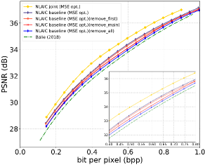
Figure 7: Ablation studies on NLAM where we gradually remove the NLAM components and re-train the model

Removing the mask branches of the first NLAM pair in the main encoder-decoders (referred to as “remove_first”) yields a PSNR drop of about 0.1dB compared to “NLAIC baseline” at the same bit rate. PSNR drop is further enlarged noticeably when removing all NLAM pairs’ mask branches in main encoder-decoders (a.k.a., “remove_main”). It gives the worst performance when further disabling the NLAM pair’s mask branches in hyperprior encoder-decoders, resulting in the traditional variational autoencoder without non-local characteristics explorations (i.e., “remove_all”).

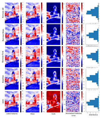
Figure 8: Prediction error with different model at similar bit rate. Column-wisely, it depicts the latent features, the predicted mean, predicted scale, normalized prediction error ( i.e., $\frac{feature-mean}{scale}$) and the distribution of the normalized prediction error from left to right plots. Each row represents a different model (e.g., various combinations of NLAM components, and contexts prediction). These figures show that with NLAM and joint contexts from hyperprior and autoregressive neighbors, the latent features capture more information (indicated by a layer dynamic range), which leads to a large scale (standard deviation of features), and the final normalized feature prediction error has the most compact distribution, which leads to the lowest bit rate.

Impacts of Joint Contexts Modeling: We further compare conditional context modeling efficiency of the model variants in Fig. 8. As we can see, with embedded NLAM and joint contexts modeling, our “NLAIC joint” could provide more powerful latent features, and more compact normalized feature prediction error, both contributing to its leading coding efficiency.

Hyperpriors $\bf{\hat{z}:}$ Hyperpriors $\hat{z}$ has noticeable contribution to the overall compression performance  [18, 5]. Its percentage decreases as the overall bit rate increases, shown in Fig. 3. The percentage of $\hat{z}$ for MSE loss optimized model is higher than the case using MS-SSIM loss optimization. Another interesting observation is that $\hat{z}$ exhibits contradictive distributions of joint and baseline models, for respective MSE and MS-SSIM loss based schemes. More explorations is highly desired in this aspect to understand the bit allocation of hyperpriors in our future study.

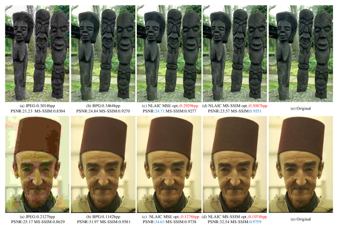
Figure 9: Visual comparison among JPEG420, BPG444, NLAIC joint MSE opt., MS-SSIM opt. and the original image from left to right. Our method achieves the best visual quality containing more texture without blocky nor blurring artifacts.

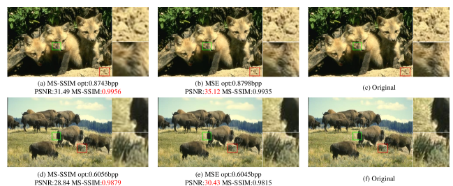
Figure 10: Illustrative reconstruction samples of respective PSNR and MS-SSIM loss optimized compression

4.4 Visual Comparison

We also evaluate our method on BSD500 [1] dataset, which is widely used in image restoration problems. Fig. 9 shows the results of different image codecs at the similar bit rate. Our NLAIC provides the best subjective quality with relative smaller bit rate.

Considering that MS-SSIM loss optimized results demonstrate much smaller PSNR at high bit rate in Fig. 4, we also show our model comparison optimized for respective PSNR and MS-SSIM loss at high bit rate scenario. We find it that MS-SSIM loss optimized results exhibit worse details compared with PSNR loss optimized models at high bit rate, as shown in Fig. 10. This may be due to the fact that pixel distortion becomes more significant at high bit rate, but structural similarity puts more weights at a fair low bit rate. It will be interesting to explore a better metric to cover the advantages of PSNR at high bit rate and MS-SSIM at low bit rate for an overall optimal efficiency.

5 Conclusion

In this paper, we proposed a non-local attention optimized deep image compression (NLAIC) method and achieve the state-of-the-art performance. Specifically, we have introduced the non-local operation to capture both local and global correlation for more compact latent feature representations. Together with the attention mechanism, we can enable the adaptive processing of latent features by allocating more bits to important area using the attention maps generated by non-local operations. Joint contexts from autoregressive spatial-channel neighbors and hyperpriors are leveraged to improve the entropy coding efficiency.

Our NLAIC outperforms the existing image compression methods, including well known BPG, JPEG2000, JPEG as well as the most recent learning based schemes [18, 5, 20], in terms of both MS-SSIM and PSNR evaluation at the same bit rate.

For future study, we can make our context model deeper to improve image compression performance. Parallelization and acceleration are important to deploy the model for actual usage in practice, particularly for mobile platforms. In addition, it is also meaningful to extend our framework for end-to-end video compression framework with more priors acquired from spatial and temporal information.

References

- [1] The berkeley segmentation dataset and benchmark.
- [2] Challenge on learned image compression 2018.
- [3] E. Agustsson, F. Mentzer, M. Tschannen, L. Cavigelli, R. Timofte, L. Benini, and L. V. Gool. Soft-to-hard vector quantization for end-to-end learning compressible representations. In Advances in Neural Information Processing Systems, pages 1141–1151, 2017.
- [4] J. Ballé, V. Laparra, and E. P. Simoncelli. End-to-end optimized image compression. arXiv preprint arXiv:1611.01704, 2016.
- [5] J. Ballé, D. Minnen, S. Singh, S. J. Hwang, and N. Johnston. Variational image compression with a scale hyperprior. arXiv preprint arXiv:1802.01436, 2018.
- [6] G. Bjontegaard. Calculation of average psnr differences between rd-curves. VCEG-M33, 2001.
- [7] A. Buades, B. Coll, and J.-M. Morel. A non-local algorithm for image denoising. In 2005 IEEE Computer Society Conference on Computer Vision and Pattern Recognition (CVPR’05), volume 2, pages 60–65. IEEE, 2005.
- [8] O. Firat, K. Cho, and Y. Bengio. Multi-way, multilingual neural machine translation with a shared attention mechanism. arXiv preprint arXiv:1601.01073, 2016.
- [9] S. Gu, L. Zhang, W. Zuo, and X. Feng. Weighted nuclear norm minimization with application to image denoising. In Proceedings of the IEEE conference on computer vision and pattern recognition, pages 2862–2869, 2014.
- [10] K. He, X. Zhang, S. Ren, and J. Sun. Deep residual learning for image recognition. In Proceedings of the IEEE conference on computer vision and pattern recognition, pages 770–778, 2016.
- [11] M. Li, W. Zuo, S. Gu, D. Zhao, and D. Zhang. Learning convolutional networks for content-weighted image compression. arXiv preprint arXiv:1703.10553, 2017.
- [12] T.-Y. Lin, M. Maire, S. Belongie, J. Hays, P. Perona, D. Ramanan, P. Dollár, and C. L. Zitnick. Microsoft coco: Common objects in context. In European conference on computer vision, pages 740–755. Springer, 2014.
- [13] D. Liu, B. Wen, Y. Fan, C. C. Loy, and T. S. Huang. Non-local recurrent network for image restoration. In Advances in Neural Information Processing Systems, pages 1680–1689, 2018.
- [14] H. Liu, T. Chen, P. Guo, Q. Shen, and Z. Ma. Gated context model with embedded priors for deep image compression. arXiv preprint arXiv:1902.10480, 2019.
- [15] M.-T. Luong, H. Pham, and C. D. Manning. Effective approaches to attention-based neural machine translation. arXiv preprint arXiv:1508.04025, 2015.
- [16] J. Mairal, F. Bach, J. Ponce, G. Sapiro, and A. Zisserman. Non-local sparse models for image restoration. In 2009 IEEE 12th International Conference on Computer Vision (ICCV), pages 2272–2279. IEEE, 2009.
- [17] F. Mentzer, E. Agustsson, M. Tschannen, R. Timofte, and L. Van Gool. Conditional probability models for deep image compression. In IEEE Conference on Computer Vision and Pattern Recognition (CVPR), volume 1, page 3, 2018.
- [18] D. Minnen, J. Ballé, and G. D. Toderici. Joint autoregressive and hierarchical priors for learned image compression. In Advances in Neural Information Processing Systems, pages 10794–10803, 2018.
- [19] A. v. d. Oord, N. Kalchbrenner, and K. Kavukcuoglu. Pixel recurrent neural networks. arXiv preprint arXiv:1601.06759, 2016.
- [20] O. Rippel and L. Bourdev. Real-time adaptive image compression. arXiv preprint arXiv:1705.05823, 2017.
- [21] G. J. Sullivan, T. Wiegand, et al. Rate-distortion optimization for video compression. IEEE signal processing magazine, 15(6):74–90, 1998.
- [22] G. Toderici, D. Vincent, N. Johnston, S.-J. Hwang, D. Minnen, J. Shor, and M. Covell. Full resolution image compression with recurrent neural networks. CoRR, abs/1608.05148, 2016.
- [23] A. Vaswani, N. Shazeer, N. Parmar, J. Uszkoreit, L. Jones, A. N. Gomez, Ł. Kaiser, and I. Polosukhin. Attention is all you need. In Advances in Neural Information Processing Systems, pages 5998–6008, 2017.
- [24] X. Wang, R. Girshick, A. Gupta, and K. He. Non-local neural networks. In Proceedings of the IEEE Conference on Computer Vision and Pattern Recognition, pages 7794–7803, 2018.
- [25] Z. Wang, E. P. Simoncelli, and A. C. Bovik. Multiscale structural similarity for image quality assessment. In The Thrity-Seventh Asilomar Conference on Signals, Systems & Computers, 2003, volume 2, pages 1398–1402. Ieee, 2003.
- [26] X. Xu, S. Liu, T. Chuang, Y. Huang, S. Lei, K. Rapaka, C. Pang, V. Seregin, Y. Wang, and M. Karczewicz. Intra block copy in hevc screen content coding extensions. IEEE Journal on Emerging and Selected Topics in Circuits and Systems, 6(4):409–419, Dec 2016.
- [27] Y. Zhang, K. Li, K. Li, B. Zhong, and Y. Fu. Residual non-local attention networks for image restoration. 2018.