Local Deep-Feature Alignment for Unsupervised Dimension Reduction

Abstract

This paper presents an unsupervised deep-learning framework named Local Deep-Feature Alignment (LDFA) for dimension reduction. We construct neighbourhood for each data sample and learn a local Stacked Contractive Auto-encoder (SCAE) from the neighbourhood to extract the local deep features. Next, we exploit an affine transformation to align the local deep features of each neighbourhood with the global features. Moreover, we derive an approach from LDFA to map explicitly a new data sample into the learned low-dimensional subspace. The advantage of the LDFA method is that it learns both local and global characteristics of the data sample set: the local SCAEs capture local characteristics contained in the data set, while the global alignment procedures encode the interdependencies between neighbourhoods into the final low-dimensional feature representations. Experimental results on data visualization, clustering and classification show that the LDFA method is competitive with several well-known dimension reduction techniques, and exploiting locality in deep learning is a research topic worth further exploring.

I Introduction

Recent years have witnessed an increase in the use of deep learning in various research domains, such as audio recognition, image and video analysis, and natural language processing. Deep learning methods can be divided into two groups: supervised learning and unsupervised learning. Supervised learning aims to learn certain classification functions based on known training samples and their labels for pattern recognition, while unsupervised learning aims to learn useful representations from unlabeled data. Both groups of methods have achieved great success, but we are particularly interested in the unsupervised learning methods because their mechanisms are closer to the learning mechanism of human brain and simpler than those of supervised methods [1].

A commonly used group of unsupervised deep-learning methods are Auto-encoders (AEs). An AE learns a single transformation matrix for embedding all the data, which means it does not discriminate between data and treats every data sample in the same way. This is coincident with some linear learning methods, such as PCA [2] and ICA [3], which usually assume that the training data obey a single Gaussian distribution. However, this assumption is not quite exact even for the same kind of data. In fact, the data used in various real-world applications often exhibit a trait of multiple Gaussian distribution. When we use multiple Gaussian models to depict the data distribution, each Gaussian model in fact reflects some local characteristic or the locality of the data set. Therefore it could be important for the AEs to preserve the local characteristic during feature learning. This concern has been supported by some previous works [4] in which an AE was equipped with a regularization term, forcing it to be sensitive only to the data variations along the data manifold where the locality was preserved. However, the regularization term was originally designed for improving robustness more than preserving locality.

A successful group of approaches to locality preservation are manifold learning algorithms [5, 6, 7, 8]. They exploit a structure called a neighbourhood graph to learn the interrelations between data and transfer the interrelations to low-dimensional space. Some algorithms assume that if some data are close to one another in the high-dimensional space, they should also be close in the low-dimensional space [6, 8]. Some algorithms assume that an unknown low-dimensional data sample can be reconstructed by its neighbours in the same way as its high-dimensional counterpart is reconstructed in the original space [5]. These objectives differ largely from that of AEs. In comparison, Local Tangent Space Alignment (LTSA) [7] computes a linear transformation for each neighbourhood to align the local tangent-space coordinates of each neighbourhood with the low-dimensional representations in a global coordinate system. Since the local tangent-space coordinates can exactly reconstruct each neighbourhood, LTSA shares more similarity with AEs. The only difference between them is that each neighbourhood in LTSA has a distinct reconstruction function and all the data in AEs share the same reconstruction function.

Enlightened by LTSA, we propose an unsupervised deep-learning framework for dimension reduction, in which the low-dimensional feature representations are obtained by aligning local features of a series of data subsets that capture the locality of the original data set. Specifically, we construct a neighbourhood for each data sample using the current sample and its neighbouring samples. Next, we stack several regularized AEs (Contractive AE or CAE [4]) together to form a deep neural network called Stacked CAE (SCAE) for mining local features from the neighbourhood. We derive the final low-dimensional feature representations by imposing a local affine transformation on the features of each neighbourhood to transfer the features from each local coordinate system to a global coordinate system. The local features learned by each SCAE reflect the deep-level characteristics of the neighbourhood, thus the proposed method can be named Local Deep-Feature Alignment (LDFA). We also derive an explicit mapping from the LDFA framework to map a new data sample to the learned low-dimensional subspace. It is worthwhile to highlight several aspects of the proposed method:

1. The locality characteristics contained in the neighbourhood can be effectively preserved by the local SCAEs.

2. The regularization term of each SCAE facilitates estimating the parameters from a neighbourhood that usually does not contain much data.

3. The number of ”variations” of the local embedding function is small [9] due to the data similarity among each neighbourhood, which reduces the difficulty in robust feature learning.

4. The local features are learned from a small amount of data in a neighbourhood, so the proposed method can work well when the data amount is not large.

The rest of this paper is organized as follows: In Section 2, we will review the related works to give the readers more insight into deep learning and locality-preserving learning. In Section 3, we will introduce the proposed method in detail. In Section 4, we will show a series of experimental results on different applications. Section 5 will present the paper’s conclusions.

II Related works

II-A Deep Learning

Deep learning algorithms (DLA) receive much attention because they can extract more representative features [10, 11, 12] from data. The current DLAs include supervised methods and unsupervised methods. The most representative supervised methods are Convolutional Neural Networks (CNNs), which are constructed by stacking three kinds of layers together, i.e., the Convolutional Layer (CL), Pooling Layer (PL), and Fully Connected Layer (FCL) [13]. The CL and PL differ from layers of regular neural networks in that the neurons in each of these two layers are only connected to a small region of the previous layer, instead of to all the neurons in a fully connected manner. This greatly reduces the number of parameters in the network and makes CNNs particularly suitable for dealing with images. However, CNNs require every data sample to have a label indicating the class tag of the sample, so they are not applicable to unsupervised feature extraction.

The most representative unsupervised deep-learning methods are AEs [14]. An AE aims to learn the low-dimensional feature representations that can best reconstruct the original data. Some researchers have enhanced AEs to increase the robustness to noise [15]. AEs are often used to construct deep neural network structures for feature extraction [16].

However, traditional AEs train a single transformation matrix for embedding all the data into low-dimensional space. Thus traditional AEs capture only the global characteristics of the data and do not consider the local characteristics. This might be inappropriate because locality has proved to be a very useful characteristic in pattern recognition [17, 18].

II-B Locality-Preserving Learning

Manifold learning methods are well known for their capabilities of preserving the local characteristics of the data set during dimension reduction [5, 6, 7, 8, 19]. The local characteristics of the original data set are contained in a structure called the neighbourhood graph, where each node representing a data sample is connected to its nearest neighbuoring nodes by arcs. The neighbourhood graph is then fed to some local estimators [9] that are capable of transferring the locality to the learned low-dimensional feature representations. Different manifold algorithms have different locality-preservation strategies.

Locally Linear Embedding (LLE) [5] reconstructs each data sample by linearly combining its neighboring data samples, and assumes the low-dimensional feature representation of the data sample can be reconstructed by its neighbours using the same combination weights. Laplacian Eigenmap (LE) [6] assumes that if two data samples are close to each other in the original data set, their low-dimensional counterparts should also be close to each other. Locality Preserving Projections (LPP) [8] shares the same objective with LE, but is realized in a linear way. Local Tangent Space Alignment (LTSA) [7] transfers the local characteristics of the data set to a low-dimensional feature space using a series of local Principal Component Analysis (PCA) applications, and then obtains the low-dimensional feature representations by aligning the local features learned by these local PCAs. In LTSA, the local estimators realized by these local PCAs are explicit and can be easily used for projecting data into low-dimensional space. This is important in dimension reduction algorithms. The locality characteristic of data can also be preserved using the joint/conditional probability distribution of data pairs based on their neighbouring structures. A typical relevant method is t-distributed stochastic neighbor embedding (t-SNE)[20] that is particularly effective in data visualization.

Some manifold-based methods encode discriminative information in neighbourhood construction. The study in [21] simultaneously extracts a pair of manifolds based on the data similarity among neighbourhoods such that the two manifolds complement each other to enhance the discriminative power of the features. In [22], the neighbourhood of each data is defined by the identity and pose information of a subject, so that the learned manifolds can be applied to person-independent human pose estimation.

However, Bengio confirmed that each of these manifold algorithms could be reformed as a single-layer nonlinear neural network [9] that fails to discover deep-level features from the original data. In addition, it does not make much sense to stack manifold learning algorithms directly as a layered structure to learn deep features because the objective functions of manifold learning methods are deliberately designed for one-layer learning. To achieve deep-level feature learning based on manifold methods, we might want to combine the locality-preservation capability of manifold methods with deep-learning methods.

II-C Combination of Deep Learning and Locality Preserving Learning

There is still no conclusion about how to encode the locality learning into the deep-learning process. Rifai [4, 23] showed that a certain kind of smoothness regularization might be useful in preserving the data locality. In [4, 23], the smoothness regularization forces AEs to be sensitive only to the data variations along the data manifold where locality is preserved. However, the smoothness regularization was originally designed for improving robustness more than preserving locality, so it only indirectly models the data locality.

Some works have been proposed to enhance deep learning with some straightforward locality-preserving constraints. A Deep Adaptive Exemplar Auto-Encoder was proposed in [24] to extract deep discriminant features by knowledge transferring. In this method, a low-rank coding regularizer transfers the knowledge of the source domain to a shared subspace with the target domain, while keeping the source and target domains well aligned through the use of locality-awareness reconstruction. This method is particularly useful in domain adaptation where the data in source domain should be labeled. [25] trained CNNs for each class of data and combined the learning results of these CNNs at the top layers using the maximal manifold-margin criterion. However, this criterion preserves discriminative information between classes by directly evaluating the Euclidean distances between the deep features learned by these CNNs. This is not quite exact because the features learned from different CNNs actually lie in different coordinate systems. In addition, all the parameters of these CNNs should be solved simultaneously in the feature-learning process, which makes the optimization process highly nonlinear and hard to solve. More importantly, the method can still not learn features without data labels.

III Local Deep Feature Alignment Framework

III-A Contractive Auto-Encoder (CAE)

The original AEs are designed for learning a feature representation from the input data sample that can be used to reconstruct the input data sample as accurately as possible [26]. Given a set of training data $\bm{{\rm X}}=[\bm{{\rm x}}_{1},\bm{{\rm x}}_{2},\dots,\bm{{\rm x}}_{N}]\in R^{D}$, the encoding (embedding) and decoding (reconstruction) process can be described as:

$$\left\{\begin{aligned} &\bm{{\rm h}}_{i}=g(\bm{{\rm Wx}}_{i}+\bm{{\rm b}})\\ &\bm{{\rm\tilde{x}}}_{i}=g(\bm{{\rm W}}^{T}\bm{{\rm h}}_{i}+\bm{{\rm c}}),\end{aligned}\right.$$ (1)

where $\bm{{\rm h}}_{i}\in R^{d}$ is the feature representation, $\bm{{\rm W}}$ describes the weight matrix of the encoding, $\bm{{\rm b}}$ and $\bm{{\rm c}}$ are the bias terms, $\bm{{\rm\tilde{x}}}_{i}$ is the reconstructed data sample and $g(\cdot)$ represents the activation function which is usually a sigmoid function:

$$g(z)=\frac{1}{1+exp(-z)}.$$ (2)

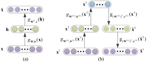
Figure 1: The Auto-encoder (AE) and a two-layer Stacked Contractive Auto-encoder (SCAE). (a) The diagram of an AE where $g_{\bm{{\rm W}},\bm{{\rm b}}}(\cdot)$ maps $\bm{{\rm x}}$ to its feature representation $\bm{{\rm h}}$ that is used to reconstruct $\bm{{\rm x}}$ as $\bm{{\rm\tilde{x}}}$ through $g_{\bm{{\rm W}}^{T},\bm{{\rm c}}}(\cdot)$. (b) The diagram of a two-layer SCAE where $g_{\bm{{\rm W}}^{(l)},\bm{{\rm b}}^{(l)}}(\cdot)(l=1,2)$ maps $\bm{{\rm x}}^{1}$ to $\bm{{\rm x}}^{3}$ that is used to obtain $\bm{{\rm\tilde{x}}}^{1}$ through $g_{(\bm{{\rm W}}^{(l)})^{T},\bm{{\rm c}}^{(l)}}(\cdot)(l=1,2)$. The superscript $l$ indicates the layer of the network.

Next, the parameters of an AE can be obtained by solving the following optimization problem:

$$\min_{\bm{{\rm h}}_{i},\bm{{\rm W}},\bm{{\rm b}},\bm{{\rm c}}}\sum_{i=1}^{N}\|\bm{{\rm h}}_{i}-g_{\bm{{\rm W}},\bm{{\rm b}}}(\bm{{\rm x}}_{i})\|^{2}+\|\bm{{\rm x}}_{i}-g_{\bm{{\rm W}}^{T},\bm{{\rm c}}}(\bm{{\rm h}}_{i})\|^{2}.$$ (3)

The functionality of an AE is depicted in Fig. 1 (a).

However, the learning process of an AE will be not robust enough in some cases, for example, when the number of data samples is much smaller than the dimension. To improve the robustness, some researchers propose to use smoothness prior to regularize the AE and thus derive the Contractive Auto-encoder (CAE) [23] whose objective function in matrix form is

$$\begin{split}&\|\bm{{\rm H}}-g_{\bm{{\rm W}},\bm{{\rm b}}}(\bm{{\rm X}})\|_{F}^{2}+\|\bm{{\rm X}}-g_{\bm{{\rm W}}^{T},\bm{{\rm c}}}(\bm{{\rm H}})\|_{F}^{2}+\\ &\lambda trace\big{(}\bm{{\rm W}}^{T}(\bm{{\rm H}}\odot(\bm{{\rm E}}-\bm{{\rm H}}))(\bm{{\rm H}}\odot(\bm{{\rm E}}-\bm{{\rm H}}))^{T}\bm{{\rm W}}\big{)},\end{split}$$ (4)

where $\bm{{\rm H}}=[\bm{{\rm h}}_{1},\dots,\bm{{\rm h}}_{N}]$, $\bm{{\rm E}}$ is a matrix in which every entry is equal to one, and $\odot$ denotes the dot product. The third term in (4) (the smoothness regularization term) keeps the feature learning process insensitive to data variations while competent for data reconstruction. This helps to extract robust low-dimensional features [23].

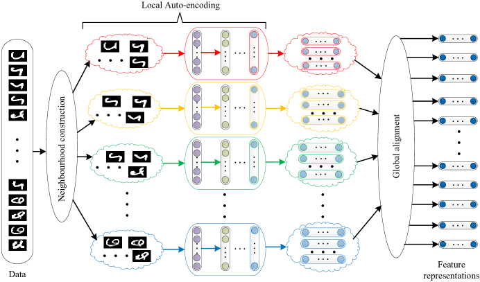
Figure 2: The basic framework of the proposed method: First, compute the neighbourhood for each data sample; Second, extract deep-level features from each neighbourhood using the local SCAEs; At last, align the local features to obtain the global feature representations.

CAEs can be used as components to form a deep neural network, where the lower layer’s output serves as the higher and adjacent layer’s input. An example of a two-layer Stacked CAE (SCAE) is shown in Fig. 1 (b). We believe the SCAE will extract more robust features than the one-layer CAE. The SCAE can be described as:

$$\begin{split}&\min_{\bm{{\rm W}},\bm{{\rm b}},\bm{{\rm c}}}\sum_{l=1}^{L}\|\bm{{\rm H}}^{l}-g_{\bm{{\rm W}}^{(l)},\bm{{\rm b}}^{(l)}}(\bm{{\rm X}}^{l})\|_{F}^{2}+\|\bm{{\rm X}}^{l}-g_{(\bm{{\rm W}}^{(l)})^{T},\bm{{\rm c}}^{(l)}}(\bm{{\rm H}}^{l})\|_{F}^{2}\\ &+\lambda trace\big{(}(\bm{{\rm W}}^{(l)})^{T}(\bm{{\rm H}}^{l}\odot(\bm{{\rm E}}-\bm{{\rm H}}^{l}))(\bm{{\rm H}}^{l}\odot(\bm{{\rm E}}-\bm{{\rm H}}^{l}))^{T}\bm{{\rm W}}^{(l)})\big{)},\\ &s.t.\quad\bm{{\rm H}}^{l}=\bm{{\rm X}}^{l+1},l=1,\ldots,L-1,\end{split}$$ (5)

where $\bm{{\rm X}}^{l}$ and $\bm{{\rm H}}^{l}$ represents the input and output of the $l_{th}$ layer respectively, and the superscript $(l)$ indicates that the parameters correspond to the $l_{th}$ layer, and we reuse $\bm{{\rm W}}$, $\bm{{\rm b}}$ and $\bm{{\rm c}}$ to represent the parameters of the SCAE.

III-B Objective Function of Local Deep-Feature Alignment

Our basic concern is to extract deep-level features from each local data subset that reflect some local characteristic of the data subset. Then we align these local features to form the global deep features.

To this end, we propose to construct a neighbourhood for each data sample that includes the sample and a number of its closest neighbouring samples. Then we use an SCAE to extract deep-level features from each neighbourhood and impose a local affine transformation on the deep features of each neighbourhood to align the features from each local coordinate system with a global coordinate system. The framework of the method is illustrated in Fig. 2.

The objective function of the method should include two parts, local deep-feature learning and global alignment of local features. For each $\bm{{\rm x}}_{i}$, we define its neighbourhood $\bm{{\rm X}}_{i}$ as $\bm{{\rm X}}_{i}=[\bm{{\rm x}}_{i},\bm{{\rm x}}_{i_{1}},\ldots,\bm{{\rm x}}_{i_{k_{i}}}]$ where $k_{i}$ is its number of neighbours. Hence the error of the SCAEs used for local feature extraction from all the neighbourhoods can be represented as:

$$\begin{split}&\sum_{i=1}^{N}\sum_{l=1}^{L}\|\bm{{\rm H}}_{i}^{l}-g_{\bm{{\rm W}}_{i}^{(l)},\bm{{\rm b}}_{i}^{(l)}}(\bm{{\rm X}}_{i}^{l})\|_{F}^{2}+\|\bm{{\rm X}}_{i}^{l}-g_{(\bm{{\rm W}}_{i}^{(l)})^{T},\bm{{\rm c}}_{i}^{(l)}}(\bm{{\rm H}}_{i}^{l})\|_{F}^{2}\\ &+\lambda trace\big{(}(\bm{{\rm W}}_{i}^{(l)})^{T}(\bm{{\rm H}}_{i}^{l}\odot(\bm{{\rm E}}-\bm{{\rm H}}_{i}^{l}))(\bm{{\rm H}}_{i}^{l}\odot(\bm{{\rm E}}-\bm{{\rm H}}_{i}^{l}))^{T}\bm{{\rm W}}_{i}^{(l)})\big{)},\\ &s.t.\quad\bm{{\rm H}}_{i}^{l}=\bm{{\rm X}}_{i}^{l+1},l=1,\ldots,L-1\end{split}$$ (6)

where the subscript $i$ is the index of the neighbourhood and other symbols have the same meanings as in formula (5).

The top-layer local deep features $\bm{{\rm H}}_{i}^{L}$ learned so far are neighbour-wise, and we need to derive the global deep features. Based on the success of LTSA, it is reasonable to assume that there exists an affine transformation between $\bm{{\rm H}}_{i}^{L}$ and their global counterparts. Let $\bm{{\rm A}}_{i}$ be the affine transformation matrix, the alignment error of each neighbourhood can be described as

$$\|\bm{{\rm H}}_{i}\bm{{\rm T}}_{i}-\bm{{\rm A}}_{i}\bm{{\rm H}}_{i}^{L}\|_{F}^{2},$$ (7)

where $\bm{{\rm T}}_{i}=\bm{{\rm I}}_{k_{i}+1}-\bm{{\rm e}}_{k_{i}+1}\bm{{\rm e}}_{k_{i}+1}^{T}/(k_{i}+1)$ moves the feature representations in $\bm{{\rm H}}_{i}$ to their geometric centre, $\bm{{\rm H}}_{i}$ is the global deep features corresponding to the $i_{th}$ neighbourhood. We need to find $\bm{{\rm A}}_{i}$ and $\bm{{\rm H}}_{i}$ such that $\bm{{\rm H}}_{i}$ preserves as much of the locality characteristics contained in $\bm{{\rm H}}_{i}^{L}$ as possible. This problem can be solved by minimizing the overall alignment error:

$$\sum_{i=1}^{N}\|\bm{{\rm H}}_{i}\bm{{\rm T}}_{i}-\bm{{\rm A}}_{i}\bm{{\rm H}}_{i}^{L}\|_{F}^{2}.$$ (8)

Combining (6) and (8) together, we describe the proposed method as the following optimization problem:

$$\begin{split}&\min_{\bm{{\rm H}}_{i},\bm{{\rm W}}_{i},\bm{{\rm b}}_{i},\bm{{\rm c}}_{i}}\big{(}\sum_{i=1}^{N}\sum_{l=1}^{L}\|\bm{{\rm H}}_{i}^{l}-g_{\bm{{\rm W}}_{i}^{(l)},\bm{{\rm b}}_{i}^{(l)}}(\bm{{\rm X}}_{i}^{l})\|_{F}^{2}+\\ &\|\bm{{\rm X}}_{i}^{l}-g_{(\bm{{\rm W}}_{i}^{(l)})^{T},\bm{{\rm c}}_{i}^{(l)}}(\bm{{\rm H}}_{i}^{l})\|_{F}^{2}+\\ &\lambda trace\big{(}(\bm{{\rm W}}_{i}^{(l)})^{T}(\bm{{\rm H}}_{i}^{l}\odot(\bm{{\rm E}}-\bm{{\rm H}}_{i}^{l}))(\bm{{\rm H}}_{i}^{l}\odot(\bm{{\rm E}}-\bm{{\rm H}}_{i}^{l}))^{T}\bm{{\rm W}}_{i}^{(l)})\big{)}\big{)}+\\ &\sum_{i=1}^{N}\|\bm{{\rm H}}_{i}\bm{{\rm T}}_{i}-\bm{{\rm A}}_{i}\bm{{\rm H}}_{i}^{L}\|_{F}^{2},\\ &s.t.\quad\bm{{\rm H}}_{i}^{l}=\bm{{\rm X}}_{i}^{l+1},l=1,\ldots,L-1\end{split}$$ (9)

where $\bm{{\rm T}}_{i}=\bm{{\rm I}}_{k_{i}+1}-\bm{{\rm e}}_{k_{i}+1}\bm{{\rm e}}_{k_{i}+1}^{T}/(k_{i}+1)$.

III-C Optimization

We adopt a two-stage strategy to optimize the problem (9). In the first stage, we learn the local deep features using a series of SCAEs. In the second stage, we align the local features to form the global feature representations.

Stage 1: In training each SCAE, to achieve optimized encoding and decoding, we can separately pre-train each CAE and optimize the deep network with the parameters initialized by the pre-trained parameters of each layer. The problem can be solved using a gradient descent algorithm with back-propagation [27]. The optimization process of an SCAE is shown in Fig. 3.

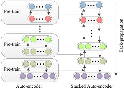
Figure 3: The optimization process of an SCAE: Pre-train each CAE layer by layer to obtain the initial parameters, then initialize the SCAE using these parameters and fine-tune the SCAE using gradient descent algorithm with back-propagation.

Stage 2: According to (8), the optimal-alignment matrix $\bm{{\rm A}}_{i}$ is given by $\bm{{\rm A}}_{i}=\bm{{\rm H}}_{i}\bm{{\rm T}}_{i}(\bm{{\rm H}}_{i}^{L})^{\dagger}$ where $(\bm{{\rm H}}_{i}^{L})^{\dagger}$ is the Moore-Penrose generalized inverse of $\bm{{\rm H}}_{i}^{L}$. Hence (8) can be rewritten as

$$\sum_{i=1}^{N}\|\bm{{\rm H}}_{i}\bm{{\rm T}}_{i}(\bm{{\rm I}}_{k_{i}+1}-(\bm{{\rm H}}_{i}^{L})^{\dagger}\bm{{\rm H}}_{i}^{L})\|_{F}^{2}.$$ (10)

Suppose $\bm{{\rm H}}=[\bm{{\rm h}}_{1},\bm{{\rm h}}_{2},\dots,\bm{{\rm h}}_{N}]\in R^{d}$ are the final feature representations where $\bm{{\rm h}}_{i}$ corresponds to $\bm{{\rm x}}_{i}$, and let $\bm{{\rm S}}_{i}$ be the 0-1 selection matrix such that $\bm{{\rm H}}\bm{{\rm S}}_{i}=\bm{{\rm H}}_{i}$. We then need to find $\bm{{\rm H}}$ to minimize the overall alignment error:

$$\sum_{i=1}^{N}\|\bm{{\rm H}}_{i}\bm{{\rm T}}_{i}(\bm{{\rm I}}_{k_{i}+1}-(\bm{{\rm H}}_{i}^{L})^{\dagger}\bm{{\rm H}}_{i}^{L})\|_{F}^{2}=\|\bm{{\rm H}}\bm{{\rm S}}\bm{{\rm M}}\|_{F}^{2},$$ (11)

where $\bm{{\rm S}}=[\bm{{\rm S}}_{1},\ldots,\bm{{\rm S}}_{N}]$ and $\bm{{\rm M}}={diag}(\bm{{\rm M}}_{1},\ldots,\bm{{\rm M}}_{N})$ with

$$\bm{{\rm M}}_{i}=(\bm{{\rm I}}_{k_{i}+1}-\bm{{\rm e}}_{k_{i}+1}\bm{{\rm e}}_{k_{i}+1}^{T}/(k_{i}+1))(\bm{{\rm I}}_{k_{i}+1}-(\bm{{\rm H}}_{i}^{L})^{\dagger}\bm{{\rm H}}_{i}^{L}).$$ (12)

Let $\bm{{\rm\Phi}}=\bm{{\rm S}}\bm{{\rm M}}\bm{{\rm M}}^{T}\bm{{\rm S}}^{T}$. Then, (11) can be rewritten as $trace(\bm{{\rm H}}\bm{{\rm\Phi}}\bm{{\rm H}}^{T})$, thus we reformulate the problem as:

$$\min_{\bm{{\rm H}}}trace(\bm{{\rm H}}\bm{{\rm\Phi}}\bm{{\rm H}}^{T}),$$ (13)

which is a typical eigenvalue problem and can be easily solved by existing methods.

Given the high-dimensional data samples $\bm{{\rm X}}=[\bm{{\rm x}}_{1},\bm{{\rm x}}_{2},\dots,\bm{{\rm x}}_{N}]$, the algorithm of the Local Deep Feature Alignment (LDFA) method can be summarized as Algorithm 1 to obtain the low-dimensional feature representations $\bm{{\rm H}}=[\bm{{\rm h}}_{1},\bm{{\rm h}}_{2},\dots,\bm{{\rm h}}_{N}]$.

Algorithm 1 The LDFA algorithm for dimension reduction.

Step 1: Compute the neighbourhood $\bm{{\rm X}}_{i}$ for each data sample $\bm{{\rm x}}_{i}$ based on the Euclidean distance metric;

Step 2: For each $\bm{{\rm X}}_{i}$, train a local deep SCAE: separately pre-train each CAE, initialize the deep SCAE using the pre-trained parameters of each layer and optimize the SCAE via the gradient-descent algorithm with back-propagation;

Step 3: Compute the top-layer local deep features $\bm{{\rm H}}_{i}^{L}$ using each SCAE’s embedding process, which can be found in (6);

Step 4: Define $\bm{{\rm S}}_{i}$ via the index set of the data contained in $\bm{{\rm X}}_{i}$, derive $\bm{{\rm M}}_{i}$ from $\bm{{\rm H}}_{i}^{L}$ following (12), and construct $\bm{{\rm S}}$ and $\bm{{\rm M}}$ ;

Step 5: Construct $\bm{{\rm\Phi}}$ using $\bm{{\rm S}}$ and $\bm{{\rm M}}$, and obtain $\bm{{\rm H}}$ by solving the eigenvalue problem (13).

III-D Embedding a New Data Sample

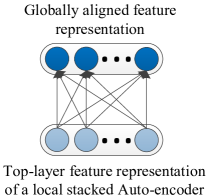
Figure 4: The fully connected network between the local feature representation of a data sample and its global counterpart.

Our proposed method can be easily extended to embed a new data sample into the learned low-dimensional subspace. We seek to construct an explicit embedding function for each local neighbourhood. Then, given a new data sample, we can find the closest sample to it in the training set, and use the corresponding embedding function to obtain the low-dimensional representation of the new data sample.

To this end, we use a one-layer fully connected feed-forward neural network to model the mapping from the top-layer local features $\bm{{\rm H}}_{i}^{L}$ to the global feature representations $\bm{{\rm H}}_{i}$. This one-layer network still exploits the sigmoid activation function and its optimization can be described as:

$$\min_{\bm{{\rm\Theta}}_{i},\bm{{\rm u}}_{i}}\left\|\bm{{\rm H}}_{i}-\frac{1}{1+exp(-(\bm{{\rm\Theta}}_{i}\bm{{\rm H}}_{i}^{L}+\bm{{\rm u}}_{i}\bm{{\rm e}}^{T}))}\right\|_{F}^{2}.$$ (14)

Fig. 4 illustrates the one-layer fully connected network.

Next, we replace the local affine-transformation matrix between $\bm{{\rm H}}_{i}^{L}$ and $\bm{{\rm H}}_{i}$ with the aforementioned fully connected network so that it is stacked on the top of the local SCAE, whose top-layer output are $\bm{{\rm H}}_{i}^{L}$. This is shown in Fig. 5.

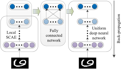
Figure 5: Construction of a new uniform deep neural network for explicitly embedding data into a low-dimensional subspace.

Note that a CAE is also realized by a one-layer neural network, which means that the fully connected network defined in (14) shares the same mathematical form with a CAE. For this reason, each SCAE, together with the corresponding fully connected network, forms a new uniform deep neural network that is able to explicitly embed a data sample into the learned low-dimensional subspace to obtain the globally aligned feature representation. The advantage of using the fully connected network for local feature alignment is that we can initialize the uniform deep neural network using the parameters of the learned SCAE and fine-tune the uniform deep network via the gradient-descent algorithm with back-propagation. The construction of a uniform deep neural network is also shown in Fig. 5. It is worthwhile to point out that the back-propagation can be used only when the local feature alignment is achieved by fully connected neural network. Therefore Algorithm 1 does not include back-propagation in local feature alignment.

Suppose each SCAE has $L$ layers. We build an $L+1$-layer deep neural network for each neighbourhood, and then initialize the parameters of the first $L$ layers with the trained SCAE and initialize the parameters of the ${L+1}_{th}$ layer with the fully connected network. Specifically, let $\bm{{\rm U}}^{i}(\cdot)$ be the explicit embedding function representing the uniform deep neural network, such that $\bm{{\rm U}}_{\bm{{\rm Q}}_{i},\bm{{\rm v}}_{i}}^{i}(\bm{{\rm X}}_{i})=\bm{{\rm H}}_{i}$. We initialize its parameters $\bm{{\rm Q}}_{i}$ and $\bm{{\rm v}}_{i}$ in the following way.

$$\left\{\begin{aligned} &{\bm{{\rm Q}}_{i}}^{(l)}={\bm{{\rm W}}_{i}}^{(l)},\quad{\bm{{\rm v}}_{i}}^{(l)}={\bm{{\rm b}}_{i}}^{(l)},\quad(l=1,\ldots,L)\\ &{\bm{{\rm Q}}_{i}}^{(l)}=\bm{{\rm\Theta}}_{i},\quad{\bm{{\rm v}}_{i}}^{(l)}=\bm{{\rm u}}_{i},\quad l=L+1,\\ \end{aligned}\right.$$ (15)

where the superscript $(l)$ indicates the parameters in the $l_{th}$ layer of the uniform deep network. Once $\bm{{\rm U}}^{i}(\cdot)$ is obtained, we can locate the nearest neighbour of a new data sample in the training set, and use the corresponding $\bm{{\rm U}}^{i}(\cdot)$ to embed the data sample into a low-dimensional subspace.

To realize the embedding of a new data sample $\bm{{\rm\tilde{x}}}$, we modify the original LDFA algorithm such that it splits into Algorithm 2 and Algorithm 3, which describe the training and embedding process respectively.

Algorithm 2 Training of LDFA for out-of-sample data embedding.

Step 1: Compute the neighbourhood $\bm{{\rm X}}_{i}$ for each data sample $\bm{{\rm x}}_{i}$ based on the Euclidean distance metric;

Step 2: For each $\bm{{\rm X}}_{i}$, train a local deep SCAE: separately pre-train each CAE, initialize the deep SCAE using the pre-trained parameters of each layer and optimize the SCAE via the gradient-descent algorithm with back-propagation;

Step 3: Compute the top-layer local deep features $\bm{{\rm H}}_{i}^{L}$ using each SCAE’s embedding process, which can be found in (6);

Step 4: Define $\bm{{\rm S}}_{i}$ via the index set of the data contained in $\bm{{\rm X}}_{i}$, derive $\bm{{\rm M}}_{i}$ from $\bm{{\rm H}}_{i}^{L}$ following (12), and construct $\bm{{\rm S}}$ and $\bm{{\rm M}}$ ;

Step 5: Construct $\bm{{\rm\Phi}}$ using $\bm{{\rm S}}$ and $\bm{{\rm M}}$, obtain $\bm{{\rm H}}$ by solving the eigenvalue problem (13);

Step 6: Build a one-layer fully connected neural network between each pair $\bm{{\rm H}}_{i}^{L}$ and $\bm{{\rm H}}_{i}$ according to (14);

Step 7: Initialize the uniform deep neural networks $\bm{{\rm U}}^{i}(\cdot)$ through (15) and fine-tune the networks using back-propagation.

Algorithm 3 Out-of-sample embedding using trained LDFA.

Step 1: Locate $\bm{{\rm\tilde{x}}}$’s nearest neighbour $\bm{{\rm x}}_{j}$ in $\bm{{\rm X}}$, and then obtain the neighbourhood $\bm{{\rm X}}_{j}$;

Step 2: Use $\bm{{\rm U}}^{j}(\cdot)$ to embed $\bm{{\rm\tilde{x}}}$ into a low-dimensional subspace and obtain its low-dimensional feature representation.

IV Experiments

We will use the proposed LDFA method in several representative applications and evaluate its performances. Dimension reduction is commonly used as a preprocessing step for subsequent data-visualization, data-clustering and data-classification tasks. Therefore, we will first examine LDFA’s image-visualization capability and clustering accuracy based on the images that have been dimension reduced using LDFA. In addition, we will determine the classification accuracy based on the LDFA feature representations. Both qualitative and quantitative experimental results will be reported, and a comparison with other existing methods will be provided.

The clustering accuracy is defined as the purity, which is computed as the ratio between the number of correctly clustered samples and the total number of samples:

$$purity(\Omega,C)=\frac{1}{N}\sum_{i}\max_{j}\{\omega_{i},c_{j}\},\quad$$

$$i=1,\dots,N_{c},j=1,\dots,N_{c},$$

where $\Omega=\{\omega_{1},\ldots,\omega_{N_{c}}\}$ is the clustered data set with $\omega_{i}$ representing the data in the $i_{th}$ cluster and $C=\{c_{1},\ldots,c_{N_{c}}\}$ is the original data set with $c_{j}$ representing the data in the $j_{th}$ class.

IV-A The Data Sets

The experiments adopt seven benchmark data sets for image visualization/clustering/classification, the data sets include the MNIST Digits , USPS Digits , Olivetti Faces , the UMist Faces , the NABirds , the Stanford Dogs , and the Caltech-256 data sets.

Table I shows the attributes of these data sets and how we use these data sets in the experiments. The attributes of each data set are the class number, the total number of data and the data dimension. Considering the computational efficiency, we are not going to use all the data for evaluation. Table I clearly indicates how many images (and per class) are involved in the experiments, and how many images are chosen for training and testing respectively. Particularly, the NABirds data set covers 400 species, but only 100 species are involved in our experiments. All the experiments are repeated 10 times, with randomly selected images in each time, and we show the statistical results of these experiments using box plot.

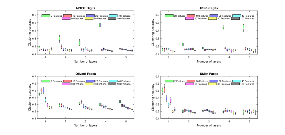
Figure 6: Clustering accuracy of the LDFA method with different numbers of layers of local SCAEs and different feature dimensions.

TABLE I: A brief description of the data sets used in the experiments.

Data Sets	Class number	Total number of data	Data dimension	Number of data in use	Number of data per class	Number of training data per class	Number of testing data per class
MNIST Digits	10	70000	784	1000	100	70	30
USPS Digits	10	11000	256	1000	100	70	30
Olivetti Faces	40	400	4096	200	5	4	1
UMist Faces	20	575	10304	360	18	15	3
NABirds	400	48000	variable	3000	30	20	10
Stanford Dogs	120	20580	variable	3600	30	20	10
Caltech-256	257	30608	variable	1,2850	50	30	20

IV-B Data Visualization and Clustering

In data visualization, the original data are embedded into a two- or three-dimensional subspace and the low-dimensional embeddings are rendered to show the spatial relationships between data samples. A good visualization result usually groups data of the same class together and separates data from different classes. In this sense, a good data-visualization result leads to high data-clustering accuracy, and viceversa. The result of data visualization and the accuracy of clustering reflect the discriminative information contained in the data, so they are commonly used for evaluating the feature representations learned by unsupervised dimension reduction algorithms.

Three factors may influence the clustering performance of the LDFA algorithm: the number of layers of the local SCAEs, the dimension of the output feature representations, and the size of the neighbourhood. Hence we want to find the proper number of layers, feature dimensions and neighbourhood size for the LDFA algorithm. First, we fix the neighbourhood size to 10, which often generates good results in many locality-preserving dimension reduction algorithms [28], and run Algorithm 1 dozens of times with different combinations of numbers of layers and feature dimensions on the MNIST Digits data set, USPS Digits data set, Olivetti Faces data set and UMist Faces data set. We perform K-means clustering [29] using the output feature representations and compute the clustering accuracies. The results of ten repeated experiments are shown in Fig. 6, where we find that four- to five-layer local SCAEs with two-dimensional features are sufficient to obtain good result for digit data sets, while one-layer local SCAEs with two- to ten-dimensional features are sufficient to get good result for face data set. Specifically, the appropriate network structures of the local SCAEs applied to the MNIST Digits, USPS Digits, UMist Faces and Olivetti Faces data sets for data visualization can be 784-300-200-150-2, 256-300-250-200-150-2, 10304-2, and 4096-2, respectively. The number of neurons in the network are smaller than that used in [30]; we believe the reason for this is that LDFA learns features from neighbourhoods, which usually contain only very similar data samples, thus it does not need a very complex network structure.

Then, using the network depth described above, we change the neighbourhood size in Algorithm 1 from 10 to 100 by intervals of 10, and the clustering accuracies of ten repeated experiments on the MNIST and USPS data sets are shown in Fig. 7. We find that the performance of the LDFA algorithm drops dramatically when the neighbourhood size increases from 10 to 20. Therefore, we believe LDFA learns discriminative local features well with relatively small neighbourhood size.

To further testify our speculation about the neighbourhood size, we perform another four tests on Caltech-256 data set that covers much more classes than MNIST and USPS data sets. In the first test, we choose 1000 samples from 50 classes with 20 samples per class and extract 59-dimension Local Binary Pattern (LBP) features [31] from these images. Then we compute the clustering accuracies based on the two dimensional features extracted by the LDFA, with the neighbourhood size varying from 10 to 90. In the second test, 2000 samples are chosen from 100 classes, and the neighbourhood size varies from 10 to 200. In the third test, 3000 samples are chosen from 150 classes, and the neighbourhood size varies from 10 to 250. In the last test, 4000 samples are selected from 200 classes, and the neighbourhood size varies from 10 to 300. The network structure is 59-30-10-2, and the experiments are also repeated 10 times with randomly selected samples each time. The clustering accuracies of these four tests are shown in Fig. 8 where we find the clustering accuracies are not increasing with bigger neighbourhood sizes when more classes are given.

Consequently, we fix the neighbourhood size in the LDFA algorithm to 10 to reduce the dimension of the aforementioned four data sets. The 2-D visualization results of the four data sets are depicted in Fig. LABEL:fig:vis_mnist, Fig. 10, Fig. 11 and Fig. 12. For comparison, we also demonstrate the visualization results of three other methods: the PCA, the t-SNE [20] and the Locally Linear Coordination (LLC) [19]. The t-SNE solves a problem known as the crowding problem during dimension reduction, which could be severe when the embedding dimension is very low. Therefore it is anticipated that the 2-D features learned by the t-SNE can well reflect the real data distribution. Fig. LABEL:fig:vis_mnist through Fig. 12 show that the LDFA are close to or comparable with t-SNE in data visualization, but better than the PCA and the LLC. This is owing to the ability of the LDFA to capture not only the global but also the local deep-level characteristics of the data sets.

To quantitatively evaluate the dimension reduction results of Fig. LABEL:fig:vis_mnist through Fig. 12, we show the clustering accuracies based on those 2-D features in Fig. 13, where we also show the clustering accuracies derived from the LTSA, the basic stacked Auto-encoders (SAE) and the SCAE. Different from other methods, the features learned by the SAE and SCAE for clustering are of 30 dimensions for good performance.In this experiment, we apply the same network structure to the SAE, SCAE and LDFA except for the dimension of the output data. The clustering on each data set is also repeated 10 times. On MNIST and USPS data sets, the LDFA is better than the PCA, LTSA, LLC, SAE and SCAE owing to the ability to capture local deep features, but inferior to the t-SNE, whose good performance is predictable from the dimension reduction results shown in Fig. LABEL:fig:vis_mnist through Fig. 12. On Olivetti and UMist Faces data sets, the LDFA achieves the best performances. It is noteworthy that the SCAE performs worse than the SAE on MNIST and USPS data sets. We think this can be explained by the characteristic of the SCAE’s regularization term to ignore the data variations that are significant even for the same kind of digits. On Olivetti and UMist Faces data sets, the performance of the SCAE is much better than the SAE because human faces share very similar structure and differenciate from one another mainly in texture, thus are more suitable to be processed by the SCAE. Also, we believe the training of the SAE needs relatively large sample set because the SAE tends to fail in capturing the data variations when the sample set is small. This explains why the clustering accuracies of the SAE on Olivetti and UMist Faces data sets are low in Fig. 13.

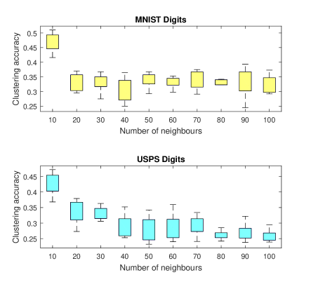
Figure 7: Clustering accuracy of the LDFA method on the MNIST data set and USPS data set with neighbourhood sizes ranging from 10 through 100.

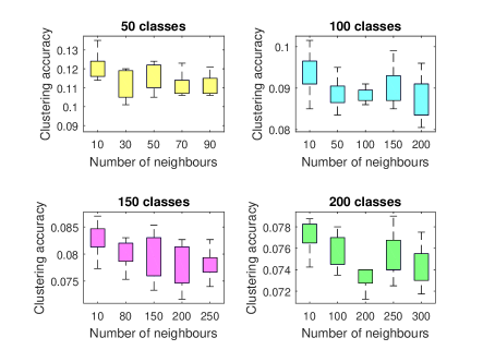
Figure 8: Clustering accuracy of the LDFA method on the Caltech-256 data set with different number of classes and neighbourhood sizes.

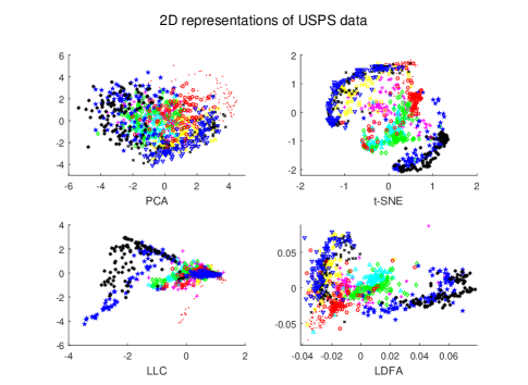
Figure 10: The 2-D visualization result of the USPS Digits data set by PCA, t-SNE, LLC and LDFA.

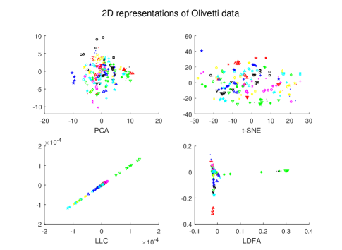
Figure 11: The 2-D visualization result of the Olivetti Faces data set by PCA, t-SNE, LLC and LDFA.

Figure 12: The 2-D visualization result of the UMist Faces data set by PCA, t-SNE, LLC and LDFA.

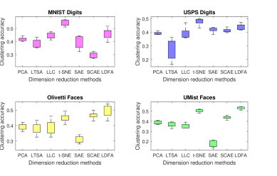
Figure 13: The clustering accuracies base on the dimension reduction results of PCA, LTSA, LLC, t-SNE, SAE, SCAE and LDFA.

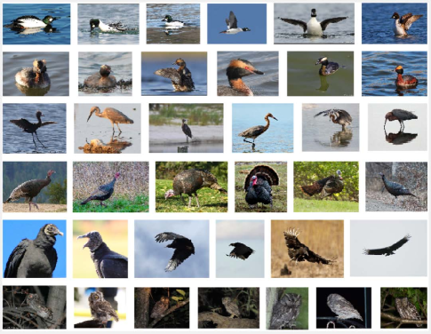
Figure 14: Some sample images selected from the NABirds data set.

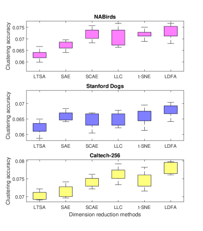
Figure 15: Clustering accuracies of LTSA, SAE, SCAE,LLC,t-SNE and LDFA on three bigger data sets.

Additionally, we perform image clustering on three bigger data sets-the NABirds, Stanford Dogs and Caltech-256, using the low-dimensional features produced by the aforementioned dimension reduction algorithms. These three data sets are much more challenging for feature learning because the foreground objects in the images are usually shown in different poses and sizes, and a large number of images are cluttered with natural scenes in the background. Some of the sample images randomly selected from the NABirds data set are shown in Fig.14, where each row represents a breed of birds. It is obvious that there exists great differences between the images of the same class. In order to improve the robustness, we extract a 59-dimension LBP feature descriptor from each image to represent it. For the SAE, SCAE and LDFA, we use the same network structure. For the LTSA, LLC and t-SNE, we use the default settings in the existing implementations. We repeat the experiment 10 times. The clustering accuracies derived from these dimension reduction algorithms are depicted in Fig. 15 where the LDFA outperforms the other five algorithms.

IV-C Data Classification

To further evaluate the discriminative information contained in the low-dimensional feature representations, we also perform image classification using the dimension-reduced data. The classification algorithms are carefully tuned so that they can generate their best results. Note that we aim to compare the feature representations learned by different methods, not to achieve the highest possible classification accuracy. Thus, we deliberately do not use some state-of-the-art classification methods.

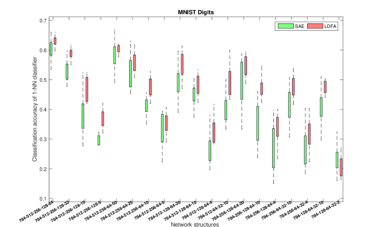
Figure 16: Classification accuracies derived from SAE and LDFA using different network structures on the MNIST data set.

Designating a very low data dimension in learning might cause the features extracted by the AEs to ”collapse” onto the same dimension [23], and this will undoubtedly influence the classification accuracy. We believe similar problem may happen to the SAE. Hence, we need to redesign the network structure for data classification. As pointed out by [32], four layers should be appropriate for an AE to learn good features. So we define 19 different four-layer network structures and implement the SAE using these structures to extract features, which are then fed into a 1-NN classifier. The classification is performed 10 times and the results are show in Fig.16 where the SAE with a 784-512-256-128-64 structure generates the best results. In addition, we plot the classification results derived from the LDFA using the 19 structures. It is clear that the LDFA outperforms the SAE with the same network structure. We will not raise the dimension of the feature representations any higher to prevent introducing the noise and instability into the feature learning [33].

Guided by similar exploration processes, we determine the network structures to be applied on the USPS, Olivetti Faces and UMist Faces data sets as 256-64-30, 4096-64 and 10304-64 respectively. Then we perform dimension reduction again using the LLC, t-SNE, SAE, SCAE and LDFA, and feed the low-dimensional feature representations to the 1-NN, random forest [34] and the naive Bayes [35] classifiers. For different dimension reduction methods, we reduce the data to the same dimension. The experiment is repeated 10 times with randomly chosen samples, and the classification accuracies can be found in Fig. 17 where the low-dimensional feature representations learned by the LDFA algorithm achieve the highest classification accuracy in most cases except for the Bayes classification on the USPS Digits and UMist Faces data sets. We believe the good performance of LDFA stems from its ability to learn not only the global characteristic but also the local deep-level characteristic of the data sets.

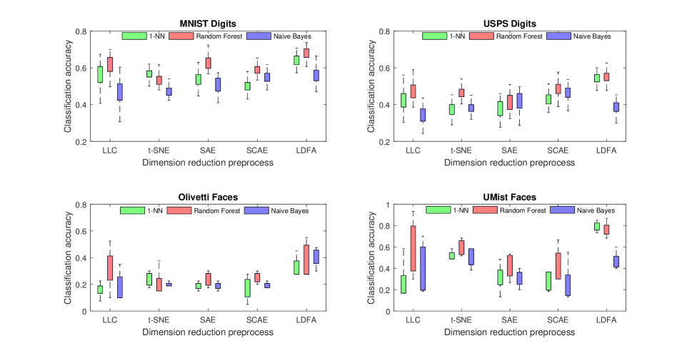
Figure 17: Classification accuracies of three common classification approaches with different dimension reduction preprocesses on the MNIST Digits, USPS Digits, Olivetti Faces and UMist Faces data sets.

In addition, we extract the LBP feature descriptors from the NABirds, Stanford Dogs and Caltech-256 data sets and conduct classification using the low-dimensional representations learned from these LBP descriptors by the LTSA, SAE, SCAE, LLC, t-SNE and the LDFA. We use the same network structure that has been adopted in Section IV-B, and this procedure is also repeated 10 times. The classification results of the 1-NN, random forest, naive Bayes, AdaBoost ensemble [36], and LDA [37] classifiers are shown in Fig. 18 through Fig. 20, which indicate that the LDFA produces the best classification results in that the features learned by LDFA generate not only the highest but also the best mean classification accuracy with respect to each classification algorithm. The only exception is the random forest classification on the Stanford Dogs data set.

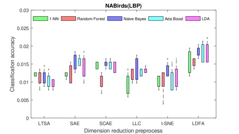
Figure 18: Classification accuracies of five common classification approaches with different dimension reduction preprocesses on the LBP features of the NABirds data set.

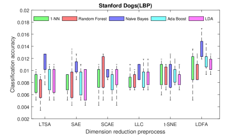
Figure 19: Classification accuracies of five common classification approaches with different dimension reduction preprocesses on the the LBP features of the Stanford Dogs data set.

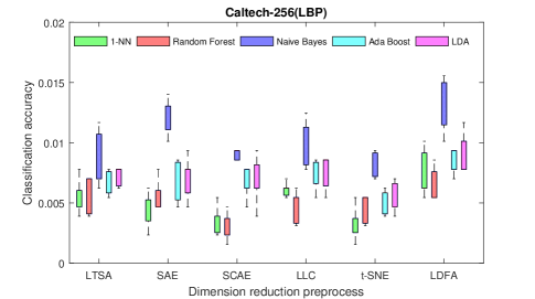
Figure 20: Classification accuracies of five common classification approaches with different dimension reduction preprocesses on the the LBP features of the Caltech-256 data set.

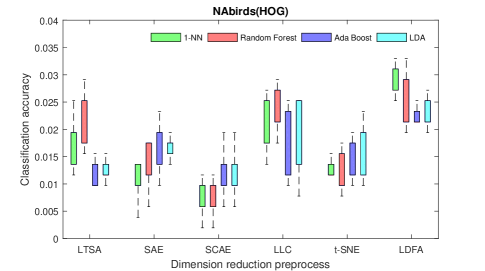
Figure 21: Classification accuracies of four common classification approaches with different dimension reduction preprocesses on the HOG features of the NABirds data set.

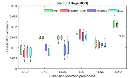
Figure 22: Classification accuracies of four common classification approaches with different dimension reduction preprocesses on the HOG features of the Stanford Dogs data set.

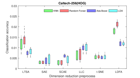
Figure 23: Classification accuracies of four common classification approaches with different dimension reduction preprocesses on the HOG features of the Caltech-256 data set.

Furthermore, we use Histogram of Oriented Gradients (HOG) [38] feature descriptors of the NABirds, Stanford Dogs and Caltech-256 data sets to evaluate the aforementioned dimension reduction methods. Specifically, we re-scale all the bird images to the same size of 512$\times$512, and set the size of the cells as 8$\times$8. Hence, the extracted HOG descriptors are of 142884 dimensions. Similarly, we resize all the dog and object images to 256$\times$256 while keeping the cell size unchanged to obtain 34596-dimension HOG descriptors. For the sake of computational convenience, the dimensions of all the HOG descriptors are reduced to 500 through PCA firstly. Then we use the LTSA, SAE, SCAE, LLC, t-SNE and LDFA to extract 30-dimension representations from the 500-dimension HOG descriptors, and conduct the classification based on the extracted representations. The experiment is also performed 10 times with randomly chosen data each time. The classification accuracies of four classification algorithms on the NABirds, Stanford Dogs and Caltech-256 data sets are demonstrated in Fig. 21 through Fig. 23 where the LDFA still produces the best results except for the AdaBoost and LDA classification on Stanford Dogs data set. Therefore, we believe the LDFA algorithm can learn more discriminative and more robust feature representations.

V Conclusion

We have proposed an unsupervised deep-learning method named Local Deep-Feature Alignment (LDFA). We define a neighbourhood for each data sample and learn the local deep features via SCAEs. Then we align the local features with global features by local affine transformations. Additionally, we provide an explicit approach to mapping new data into the learned low-dimensional subspace.

The proposed LDFA method has been used as a pre-processing step for image visualization, image clustering and image classification in our experiments. We found that SCAE could extract discriminative local deep features robustly from a small number of data samples (neighbourhood) with few network layers. These experimental results persuaded us that using SCAE to capture the local characteristics of data sets would improve the performance of the unsupervised deep-learning method.

Jian Zhang received the Ph.D. degree from Zhejiang University, Zhejiang, China. He is currently an Associate Professor with the School of Science and Technology, Zhejiang International Studies University, Hangzhou, China. From 2009 to 2011, he was with Department of Mathematics of Zhejiang university as a Post-doctoral Research Fellow. In 2016, he had been doing research on machine learning at Simon Fraser University (SFU) as a Visiting Scholar. His research interests include but not limited to machine learning, computer animation and image processing. He serves as a reviewer of several prestigious journals in his research domain.

Jun Yu (M’13) received the B.Eng. and Ph.D. degrees from Zhejiang University, Zhejiang, China. He is currently a Professor with the School of Computer Science and Technology, Hangzhou Dianzi University, Hangzhou, China. He was an Associate Professor with the School of Information Science and Technology, Xiamen University, Xiamen, China. From 2009 to 2011, he was with Nanyang Technological University, Singapore. From 2012 to 2013, he was a Visiting Researcher at Microsoft Research Asia (MSRA). Over the past years, his research interests have included multimedia analysis, machine learning, and image processing. He has authored or coauthored more than 60 scientific articles. In 2017 Prof. Yu received the IEEE SPS Best Paper Award. Prof. Yu has (co-)chaired several special sessions, invited sessions, and workshops. He served as a program committee member or reviewer of top conferences and prestigious journals. He is a Professional Member of the Association for Computing Machinery (ACM) and the China Computer Federation (CCF).

Dacheng Tao (F 15) is Professor of Computer Science and ARC Laureate Fellow in the School of Information Technologies and the Faculty of Engineering and Information Technologies, and the Inaugural Director of the UBTECH Sydney Artificial Intelligence Centre, at the University of Sydney. He mainly applies statistics and mathematics to Artificial Intelligence and Data Science. His research interests spread across computer vision, data science, image processing, machine learning, and video surveillance. His research results have expounded in one monograph and 500+ publications at prestigious journals and prominent conferences, such as IEEE T-PAMI, T-NNLS, T-IP, JMLR, IJCV, NIPS, ICML, CVPR, ICCV, ECCV, ICDM; and ACM SIGKDD, with several best paper awards, such as the best theory/algorithm paper runner up award in IEEE ICDM 07, the best student paper award in IEEE ICDM 13, the distinguished student paper award in the 2017 IJCAI, the 2014 ICDM 10-year highest-impact paper award, and the 2017 IEEE Signal Processing Society Best Paper Award. He received the 2015 Australian Scopus-Eureka Prize, the 2015 ACS Gold Disruptor Award and the 2015 UTS Vice-Chancellor s Medal for Exceptional Research. He is a Fellow of the IEEE, AAAS, OSA, IAPR and SPIE.

References

- [1] Y. LeCun, Y. Bengio, and G. Hinton, “Deep learning,” Nature, vol. 521, no. 7553, pp. 436–444, 2015.
- [2] K. Pearson, “Liii. on lines and planes of closest fit to systems of points in space,” The London, Edinburgh, and Dublin Philosophical Magazine and Journal of Science, vol. 2, no. 11, pp. 559–572, 1901.
- [3] A. Hyvärinen, J. Karhunen, and E. Oja, Independent component analysis. John Wiley & Sons, 2004, vol. 46.
- [4] G. Alain, Y. Bengio, and S. Rifai, “Regularized auto-encoders estimate local statistics,” Proceedings of CoRR, vol. abs/1211.4246, no. 11, pp. 1–17, 2012.
- [5] S. T. Roweis and L. K. Saul, “Nonlinear dimensionality reduction by locally linear embedding,” Science, vol. 290, no. 5500, pp. 2323–2326, 2000.
- [6] M. Belkin and P. Niyogi, “Laplacian eigenmaps and spectral techniques for embedding and clustering,” in Advances in neural information processing systems, 2002, pp. 585–591.
- [7] Z. Zhang and H. Zha, “Principal manifolds and nonlinear dimensionality reduction via tangent space alignment,” SIAM journal on scientific computing, vol. 26, no. 1, pp. 313–338, 2004.
- [8] X. He and P. Niyogi, “Locality preserving projections,” in Advances in neural information processing systems, 2004, pp. 153–160.
- [9] Y. Bengio, “Learning deep architectures for ai,” Foundations and trends® in Machine Learning, vol. 2, no. 1, pp. 1–127, 2009.
- [10] C. Jia, M. Shao, and Y. Fu, “Sparse canonical temporal alignment with deep tensor decomposition for action recognition,” IEEE Transactions on Image Processing, vol. 26, no. 2, pp. 738–750, 2017.
- [11] G. Li and Y. Yu, “Visual saliency detection based on multiscale deep cnn features,” IEEE Transactions on Image Processing, vol. 25, no. 11, pp. 5012–5024, 2016.
- [12] D. Liu, Z. Wang, B. Wen, J. Yang, W. Han, and T. S. Huang, “Robust single image super-resolution via deep networks with sparse prior,” IEEE Transactions on Image Processing, vol. 25, no. 7, pp. 3194–3207, 2016.
- [13] K. He, X. Zhang, S. Ren, and J. Sun, “Spatial pyramid pooling in deep convolutional networks for visual recognition,” IEEE Transactions on Pattern Analysis and Machine Intelligence, vol. 37, no. 9, pp. 1904–1916, 2015.
- [14] S. C. AP, S. Lauly, H. Larochelle, M. Khapra, B. Ravindran, V. C. Raykar, and A. Saha, “An autoencoder approach to learning bilingual word representations,” in Advances in Neural Information Processing Systems, 2014, pp. 1853–1861.
- [15] G. Alain and Y. Bengio, “What regularized auto-encoders learn from the data-generating distribution.” Journal of Machine Learning Research, vol. 15, no. 1, pp. 3563–3593, 2014.
- [16] P. Vincent, H. Larochelle, I. Lajoie, Y. Bengio, and P.-A. Manzagol, “Stacked denoising autoencoders: Learning useful representations in a deep network with a local denoising criterion,” Journal of Machine Learning Research, vol. 11, no. Dec, pp. 3371–3408, 2010.
- [17] L. Liu, M. Yu, and L. Shao, “Unsupervised local feature hashing for image similarity search,” IEEE transactions on cybernetics, vol. 46, no. 11, pp. 2548–2558, 2016.
- [18] J. Tang, L. Shao, X. Li, and K. Lu, “A local structural descriptor for image matching via normalized graph laplacian embedding,” IEEE transactions on cybernetics, vol. 46, no. 2, pp. 410–420, 2016.
- [19] S. T. Roweis, L. K. Saul, and G. E. Hinton, “Global coordination of local linear models,” in Advances in neural information processing systems, 2002, pp. 889–896.
- [20] L. v. d. Maaten and G. Hinton, “Visualizing data using t-sne,” Journal of Machine Learning Research, vol. 9, no. Nov, pp. 2579–2605, 2008.
- [21] Y. Su, S. Li, S. Wang, and Y. Fu, “Submanifold decomposition,” IEEE Transactions on Circuits and Systems for Video Technology, vol. 24, no. 11, pp. 1885–1897, 2014.
- [22] S. Yan, H. Wang, Y. Fu, J. Yan, X. Tang, and T. S. Huang, “Synchronized submanifold embedding for person-independent pose estimation and beyond,” IEEE Transactions on Image Processing, vol. 18, no. 1, pp. 202–210, 2009.
- [23] S. Rifai, P. Vincent, X. Muller, X. Glorot, and Y. Bengio, “Contractive auto-encoders: Explicit invariance during feature extraction,” in Proceedings of the 28th International Conference on Machine Learning, 2011, pp. 833–840.
- [24] M. Shao, Z. Ding, H. Zhao, and Y. Fu, “Spectral bisection tree guided deep adaptive exemplar autoencoder for unsupervised domain adaptation.” in AAAI, 2016, pp. 2023–2029.
- [25] J. Lu, G. Wang, W. Deng, P. Moulin, and J. Zhou, “Multi-manifold deep metric learning for image set classification,” in Proceedings of the IEEE Conference on Computer Vision and Pattern Recognition, 2015, pp. 1137–1145.
- [26] P. Baldi, “Autoencoders, unsupervised learning, and deep architectures.” ICML unsupervised and transfer learning, vol. 27, no. 37-50, p. 1, 2012.
- [27] Y. Chauvin and D. E. Rumelhart, Backpropagation: Theory, architectures, and applications. Hove,United Kingdom: Psychology Press, 1995.
- [28] A. Smith, H. Zha, and X.-m. Wu, “Convergence and rate of convergence of a manifold-based dimension reduction algorithm,” in Advances in Neural Information Processing Systems, 2008, pp. 1529–1536.
- [29] J. A. Hartigan and M. A. Wong, “Algorithm as 136: A k-means clustering algorithm,” Journal of the Royal Statistical Society. Series C (Applied Statistics), vol. 28, no. 1, pp. 100–108, 1979.
- [30] G. E. Hinton and R. R. Salakhutdinov, “Reducing the dimensionality of data with neural networks,” Science, vol. 313, no. 5786, pp. 504–507, 2006.
- [31] T. Ahonen, A. Hadid, and M. Pietikainen, “Face description with local binary patterns: Application to face recognition,” IEEE transactions on pattern analysis and machine intelligence, vol. 28, no. 12, pp. 2037–2041, 2006.
- [32] L. Van Der Maaten, E. Postma, and J. Van den Herik, “Dimensionality reduction: a comparative review,” Journal of Machine Learning Research, vol. 10, pp. 66–71, 2009.
- [33] E. Levina and P. J. Bickel, “Maximum likelihood estimation of intrinsic dimension,” in Advances in neural information processing systems, 2005, pp. 777–784.
- [34] T. K. Ho, “Random decision forests,” in Proceedings of the Third International Conference on Document Analysis and Recognition, vol. 1. IEEE, 1995, pp. 278–282.
- [35] C. Elkan, “Boosting and naive bayesian learning,” Department of Computer Science and Engineering, University of California, San Diego La Jolla, California 92093-0114, Tech. Rep. CS97-557, 1997.
- [36] H.-B. Shen and K.-C. Chou, “Ensemble classifier for protein fold pattern recognition,” Bioinformatics, vol. 22, no. 14, pp. 1717–1722, 2006.
- [37] R. A. Fisher, “The use of multiple measurements in taxonomic problems,” Annals of human genetics, vol. 7, no. 2, pp. 179–188, 1936.
- [38] N. Dalal and B. Triggs, “Histograms of oriented gradients for human detection,” in Proceedings of the IEEE Conference on Computer Vision and Pattern Recognition, vol. 1. IEEE, 2005, pp. 886–893.