Diamagnetic levitation and thermal gradient driven motion of graphite

Abstract

We theoretically study the diamagnetic levitation and the thermal-driven motion of graphite. Using the quantum-mechanically derived magnetic susceptibility, we compute the equilibrium position of levitating graphite over a periodic arrangement of magnets, and investigate the dependence of the levitation height on the susceptibility and the geometry. We find that the levitation height is maximized at a certain period of the magnets, and the maximum height is then linearly proportional to the susceptibility of the levitating object. We compare the ordinary AB-stacked graphite and a randomly stacked graphite, and show that the latter exhibits a large levitation length particularly in low temperatures, because of its diamagnetism inversely proportional to the temperature. Finally, we demonstrate that the temperature gradient moves the levitating object towards the high temperature side, and estimate the generated force as a function of susceptibility.

I Introduction

Diamagnetism is a property of material to repel a magnetic field. Materials with strong diamagnetism can even levitate freely over a magnet, and it is called the diamagnetic levitation. The best known example of this is the Meissner effect of superconductors, while normal-state diamagnetic materials can also levitate under an appropriate experimental setup. The stable levitation of graphite and bismuth was first demonstrated in 1930’s.Braunbek (1939) It was more recently shown that even a piece of wood and plastic Beaugnon and Tournier (1991) and also a living frog Berry and Geim (1997); Simon and Geim (2000) and cell Winkleman et al. (2004) are able to levitate with a powerful magnet, due to their tiny diamagnetism.

Graphite is one of the strongest diamagnetic materials among natural substances, and its anomalous magnetic susceptibility originates from the orbital motion of the Dirac-like electrons. McClure (1956); Fukuyama and Kubo (1970); Sharma et al. (1974); Fukuyama (2007); Koshino and Ando (2007a) The diamagnetic levitation of graphite was also extensively studied and various applications have been proposed. Waldron (1966); Moser and Bleuler (2002); Moser et al. (2002); Boukallel et al. (2003); Cansiz and Hull (2004); Li et al. (2006); Liu et al. (2008); Mizutani et al. (2012); Kustler (2012); Kobayashi and Abe (2012); Hilber and Jakoby (2013); Su et al. (2015); Kang et al. (2018); Niu et al. (2018); Ewall-Wice et al. (2019) A typical experimental setup used for the diamagnetic levitation is a checkerboard arrangement of NdFeB magnet as shown in Fig. 1, where the alternating pattern of magnetic poles generates a magnetic field gradient to support a diamagnetic object in a free space. Moser et al. (2002); Kustler (2012); Mizutani et al. (2012); Kobayashi and Abe (2012); Niu et al. (2018); Ewall-Wice et al. (2019) A recent experiment performed a detailed measurement of the levitation height of a graphite piece in this geometry. Kobayashi and Abe (2012) The same experiment also demonstrated an optical motion control in the diamagnetic levitation, where the levitating graphite is moved towards the photo irradiated spot, motivated by the photothermal change in the magnetic susceptibility. Kobayashi and Abe (2012); Ewall-Wice et al. (2019)

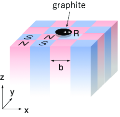
Figure 1: Diamagnetic levitation of graphite on a checkerboard array of magnets.

In this paper, we present a detailed theoretical study of the diamagnetic levitation and the thermal-driven motion of graphite. Using the orbital diamagnetic susceptibility $\chi$ calculated from the standard band model, we compute the equilibrium levitating position of a diamagnetic object over the checkerboard magnet, and obtain the levitation height as a function of $\chi$, the checkerboard period, and the size of the object. We find that the levitation height is maximized at a certain period of the magnets, and the maximum height is then linearly proportional to $\chi$. Finally we demonstrate that the temperature gradient moves the levitating object to the high temperature side, and estimate the generated force as a function of susceptibility.

In addition to the ordinary graphite with AB (Bernal) stacking structure [Fig. 2(a)], we also consider a randomly stacked graphite [Fig. 2(b)], in which successive graphene layers are stacked with random in-plane rotations. There the reduced interlayer coupling leads to a strong diamagnetism inversely proportional to the temperature Ominato and Koshino (2013), and therefore a large levitation length is achieved in low temperatures. In the liquid nitrogen temperature (77K), for example, the maximum levitation length is found to be about 5 mm, which is 10 times as large as the typical levitation height of the AB-stacked graphite.

The paper is organized as follows. In Sec. II, we briefly introduce the magnetic susceptibility of AB-stacked graphite and randomly-stacked graphite. We then calculate the magnetic levitation of general diamagnetic objects in the checkerboard magnet array in Sec. III. We consider the thermal-gradient force in magnetic levitation in Sec. IV. A brief conclusion is given in Sec. V. The susceptibility calculation for the AB-stacked graphite is presented in Appendix A.

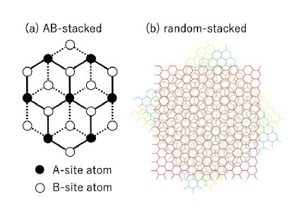
Figure 2: Atomic structure of (a) AB-stacked graphite and (b) randomly stacked graphite.

II Magnetic Susceptibility

We calculate the magnetic susceptibility of graphite using the quantum mechanical liner-response formula Fukuyama (1971), and the standard band model. Wallace (1947); McClure (1957); Slonczewski and Weiss (1958); Dresselhaus and Dresselhaus (2002) The detail description of the calculation is presented in Appendix A. Figure 3(a) plots the susceptibility $\chi$ of AB-stacked graphite as a function of temperature. Throughout the paper, we define $\chi$ as the dimensionless susceptibility in the SI unit (the perfect diamagnetism is $\chi=-1$). In decreasing temperature, $\chi$ slowly increases nearly in a logarithmic manner, and finally saturate around $T\sim 50$ K. The logarithmic increase is related to the quadratic band touching in the in-plane dispersion, and the saturation caused by the semimetallic band structure of graphite, as argued in Appendix A.

The susceptibility of random-stacked graphite is approximately given by that of an infinite stack of independent monolayer graphenes. This simplification is valid when the twist angle $\theta$ between adjacent layers is not too small ($\theta\gg 1^{\circ}$). If a small twist angle happens to occur somewhere in the random stack, these two layers are strongly coupled to form flat bands Bistritzer and MacDonald (2011); de Laissardiere et al. (2012), and do not participate in the large diamagnetism given by the nearly-independent graphene part. By neglecting this, the susceptibility at the charge neutral point is explicitly written as Ominato and Koshino (2013)

$$\chi=\frac{-1}{1+k_{B}T/\Delta},$$ (1)

where $\Delta$ is a characteristic energy scale defined by

$$\Delta=\frac{g_{v}g_{s}}{6}\left(\frac{v}{c}\right)^{2}\frac{e^{2}}{4\pi\epsilon_{0}d}\approx 0.03\ \mbox{meV},$$ (2)

and $c$ is the light velocity. The susceptibility is nearly proportional to $1/T$ in $k_{B}T\ll\Delta$ ($T\gg 0.35$ K). As plotted in Fig. 3(b), the susceptibility of random-stacked graphite is much greater than that of AB-stacked graphite particularly in the low-temperature regime. The real system should have some disorder potential, and then we expect that $\chi$ saturates at $k_{B}T\sim\Gamma$, where $\Gamma$ is the broadening broadening near the Dirac point of graphene.

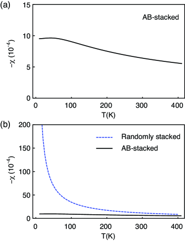
Figure 3: (a) Temperature dependence of the total susceptibility $\chi$ of AB-stacked graphite with $\mu=0$. (b) Similar plot for the randomly stacked graphite (blue dashed), compared to that of AB-stacked graphite (black solid).

III Magnetic Levitation

We consider magnetic levitation of graphite in the geometry illustrated in Fig. 4(a). Here the N-pole and S-pole of square-shaped magnets of size $b$ are alternately arranged in a checkerboard pattern. We place a round-shaped graphite disk of radius $R$ and the thickness $w$ right above a grid point where four magnet blocks meet. We assume the surface of the magnet top and the graphite disk is perpendicular to the gravitational direction, $z$. The graphite is attracted to the grid point where the magnetic field is the weakest.

When the magnetic field distribution $\mathbf{B}=\mathbf{B}(x,y,z)$ is given, the total energy $U$ of the graphite disk is given by

$$U=Mgz+w\int_{S}dxdy\frac{-1}{2\mu_{0}}\chi B_{z}(x,y,z)^{2},$$ (3)

Here $g$ is the gravitational acceleration, $M$ is the mass of the disk, $S$ is the area of the disk, $\chi$ is the magnetic susceptibility of graphite, and $z$ is the vertical position of the disk. We assumed the thickness of graphite is thin enough. The equilibrium position $z=z_{\rm lev}$ (i.e., the levitation length) is obtained by solving $\partial U/\partial z=0$, or

$$\left\langle\frac{dB_{z}^{2}}{dz}\right\rangle_{S}=2\mu_{0}\frac{\rho g}{\chi}.$$ (4)

Here $\rho\approx 2.2$ g/cm³ is the mass density of graphite, and $\langle\cdots\rangle_{S}$ is the average over the graphite area. For the magnetic levitation, therefore, the squared magnetic field gradient $dB_{z}^{2}/dz$ matters more than the absolute field amplitude itself.

Now we consider an infinite checkerboard arrangement of square blocks of NdFeB magnet. The $z$-component of the magnetic field generated by a single block can be calculated by the formula, Camacho and Sosa (2013)

$$B^{(1)}_{z}(x,y,z)=-\frac{B_{0}}{2\pi}[F_{1}(-x,y,z)+F_{1}(-x,y,-z)$$

$$+F_{1}(-x,-y,z)+F_{1}(-x,-y,-z)+F_{1}(x,y,z)$$

$$+F_{1}(x,y,-z)+F_{1}(x,-y,z)+F_{1}(x,-y,-z)],$$ (5)

with

$$F_{1}(x,y,z)=$$

$$\arctan\frac{\left(x+\frac{b_{x}}{2}\right)\left(y+\frac{b_{y}}{2}\right)}{\left(z+\frac{b_{z}}{2}\right)\sqrt{\left(x+\frac{b_{x}}{2}\right)^{2}+\left(y+\frac{b_{y}}{2}\right)^{2}+\left(z+\frac{b_{z}}{2}\right)^{2}}},$$ (6)

where $B_{0}$ is the amplitude of the surface magnetic field, and $b_{x}$, $b_{y}$ and $b_{z}$, are the side lengths, and the $N$ and $S$ poles of the magnet correspond to the faces of $z=b_{z}/2$ and $-b_{z}/2$, respectively. The total magnetic field $B_{z}(x,y,z)$ is obtained as an infinite sum of $B^{(1)}_{z}$ over all the blocks composing the checkerboard array. We take $B_{0}=500$ mT as a typical value for NdFeB magnet, and assume the square and long shape, i.e., $b_{x}=b_{y}\equiv b$, and $b_{z}\to\infty$.

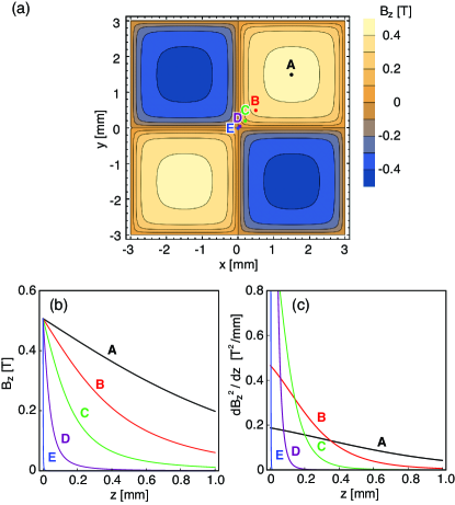
Figure 4: (a) Distribution of $B_{z}$ on $xy$-plane, at $0.2$ mm height over an infinite checkerboard magnet array with $b=3$ mm. (b) Plot of $B_{z}$ as functions of $z$, at the five points $A=(1.5,1.5),B=(0.5,0.5),C=(0.2,0.2),D=(0.05,0.05)$ and $E=(0.001,0.001)$ (in units of mm) which are indicated in the panel (a). (c) Similar plot for $dB_{z}^{2}/dz$.

Figure 4(a) shows the actual distribution of $B_{z}$ at $0.2$ mm height from the surface for $b=3$ mm magnet array. Figures 4(b) and (c) are the plots of $B_{z}$ and $dB_{z}^{2}/dz$ as functions of $z$, respectively, at the five points $A=(1.5,1.5),B=(0.5,0.5),C=(0.2,0.2),D=(0.05,0.05)$ and $E=(0.001,0.001)$ in units of mm. Here the coordinate origin is taken to a grid point on the upper surface of the arranged magnets. At any $xy$-points, the magnetic field $B_{z}$ exponentially decays in $z$, and its decay length is shorter when closer to the origin, and so does $dB_{z}^{2}/dz$.

The averaged squared magnetic field $\langle B_{z}^{2}\rangle_{S}$ can also be well approximated by an exponential function in $z$ as,

$$\langle B_{z}^{2}\rangle_{S}\approx\alpha B_{0}^{2}e^{-z/\lambda},$$ (7)

where $\alpha$ is the dimensionless constant of the order of 1, and $\lambda$ is the length scale determined by the geometry. Then Eq. (4) is explicitly solved as

$$z_{\rm lev}\approx\lambda\log\frac{\alpha\lambda_{0}}{\lambda}$$ (8)

with the characteristic length,

$$\lambda_{0}=\frac{|\chi|B_{0}^{2}}{2\mu_{0}\rho g}.$$ (9)

The negative solution of Eq. (8) indicates that the graphite does not levitate.

If the graphite radius $R$ is much greater than the magnet grid size $b$, in particular, $\langle B_{z}^{2}\rangle_{S}$ is replaced by the average value over whole $xy$-plane, and then $\lambda$ depends solely on $b$ (not on $R$). In this limit, we have $\alpha\sim 0.7$ and $\lambda\sim\eta b$ with $\eta\sim 0.11$. Figure 5(a) plots the levitation height $z_{\rm lev}$ as a function of the grid size $b$, calculated for different $\chi$’s in this limit, The solid curves are the numerical solution of Eq. (4), and the dashed curves are the approximate expression Eq. (8) with $\alpha=0.7$ and $\eta=0.11$. The curves with different $\chi$’s are just scaled through the length parameter $\lambda_{0}$. Here we take $-\chi=2,5,10,20,50(\times 10^{-4})$ ($\rho$ is fixed), which give $\lambda_{0}$ is $0.9,2.2,4.5,9.0,22.4$mm, respectively. As is obvious from its analytic form, the approximate curve peaks at $b=\alpha\lambda_{0}/(\eta e)\approx 2.3\lambda_{0}$ ($e$ is the base of the natural logarithm), where the levitation height takes the maximum value,

$$z^{\rm(max)}_{\rm lev}=\frac{\alpha\lambda_{0}}{e}\approx 0.26\lambda_{0}.$$ (10)

We see that the approximation fails for $b$ greater than the peak position. This is because Eq. (7) is not accurate $z<\lambda$, where the actual $\langle B_{z}^{2}\rangle_{S}$ becomes higher than the approximation. The gradient $d\langle B_{z}^{2}\rangle_{S}/dz$ at $z=0$ is given by $-B_{0}^{2}/(\eta^{\prime}b)$ with $\eta^{\prime}\sim 0.05$, and it gives the vanishing point of $z_{\rm lev}$ at $b=\lambda_{0}/\eta^{\prime}\sim 20\lambda_{0}$. This is much further than the end of the approximate curve, $b=\alpha\lambda_{0}/\eta\approx 6.2\lambda_{0}$. The approximate formula is still useful for qualitative estimation of the maximum levitation length $z^{\rm(max)}$.

The important fact is that all the length scales of the system, such as the levitation height and the grid period, are scaled by a single parameter $\lambda_{0}$ [Eq. (9)], which is proportional to $\chi$. If $\chi$ is doubled, therefore, we have the same physics with all the length scale doubled. For the typical susceptibility of AB-stacked graphite at the room temperature, $\chi=-5\times 10^{-4}$, the characteristic length becomes $\lambda_{0}=2.23$ mm, and we have $z^{\rm(max)}=0.65$ mm at $b=7.5$ mm. For the randomly-stacked graphite at 77K, on the other hand, the susceptibility is about $\chi=-45\times 10^{-4}$, giving $z^{\rm(max)}=5.9$ mm at $b=68$ mm.

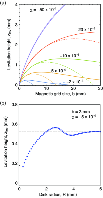
Figure 5: (a) Levitation height $z_{\rm lev}$ as a function of the magnetic grid size $b$, calculated for different $\chi$’s with the limit of $R\gg b$. Solid curves are the numerical solution of Eq. (4), and the dashed curves are the approximate expression Eq. (8). (b) $R$-dependence of the levitation height in $\chi=-5\times 10^{-4}$ and the magnetic grid with $b=3$ mm. The horizontal dashed line indicates the asymptotic value in $R\to\infty$.

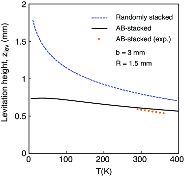
Figure 6: Temperature dependence of the levitation height of the AB-stacked graphite (blue dashed) and randomly-stacked graphite (black solid) of radius $R=1.5$ mm, in the magnetic grid with $b=3$ mm. The orange dots represent the levitation length of AB-stack graphite measured in the experiment. Kobayashi and Abe (2012)

The levitation also depends on the size of the disk. Figure 5(b) shows the levitation height as a function of the disk radius $R$, at $\chi=-5\times 10^{-4}$ and $b=3$ mm. In increasing $R$, the levitation length first monotonically increases, and then eventually approaches to the asymptotic value (dashed line) argued above, after some oscillation. The monotonic increasing region corresponds to the disk size smaller than the magnet grid size $b$. There a smaller disk has a smaller levitation, because as seen in Fig.  4(c), $dB_{z}^{2}/dz$ near the origin quickly decays in $z$, so a tiny disk can levitate only in a small distance to catch the finite $dB_{z}^{2}/dz$.

In Fig. 6, we show the temperature dependence of the levitation length $z_{\rm lev}$ of the AB-stacked graphite and randomly stacked graphite, with a disk radius $R=1.5$ mm. In a fixed geometry, $z_{\rm lev}$ is proportional to $\log|\chi|$ according to Eq. (8). We see that the $z_{\rm lev}$ of AB-stacked graphite shows a similar temperature dependence to the susceptibility itself [Fig. 3(a)]. The randomly stacked graphite exhibits a $\log T$ behavior because $z_{\rm lev}\propto\log|\chi|$ and $\chi\propto 1/T$. The orange dots in Fig. 6 indicate the levitation length of AB-stack graphite measured in the experiment. Kobayashi and Abe (2012) We can see a good quantitative agreement between the simulation and experiment without any parameter fitting. The simulation underestimates the slope of the temperature dependence, suggesting that the susceptibility in the real system decreases more rapidly in temperature than in our model calculation. A possible reason for this would be the effect of phonon scattering, which increases the energy broadening $\Gamma$ in higher temperature and reduces the susceptibility.

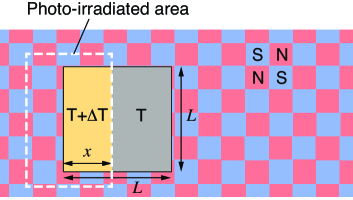
Figure 7: Setup of the thermal-driven motion of levitating graphite. A square-shaped graphite piece levitates on the magnet checkerboard and it is partially heated by photo irradiation.

IV Thermal gradient driven motion

A graphite piece much larger than the magnet size $b$ freely moves along the horizontal direction while floating over the magnets, because it covers a number of magnetic periods and the total energy hardly depends on the $xy$ position. Now we consider a situation illustrated in Fig. 7, where a part of the levitating graphite piece is heated by photo irradiation. We assume that the irradiated area is fixed to the rest frame of the magnets, and consider the movement of graphite against it. In the experiment, it was shown that the graphite is attracted to the photo irradiated region. Kobayashi and Abe (2012); Ewall-Wice et al. (2019) This can be understood that the graphite minimizes the total energy by moving to the high temperature area, where the diamagnetism is smaller so that the energy cost is lower under the same magnetic field.

We can estimate the magnitude of the thermal gradient force as following. We consider a $L\times L$ square-shaped graphite piece with thickness $w$, and assume that the graphite in the irradiated area is instantly heated up to temperature $T+\Delta T$, while otherwise the temperature remains $T$, as in Fig. 7. The length of the high temperature region is denoted by a variable $x$. i.e., when the graphite is moved to the left, then $x$ increases. We neglect the heat transport on the graphite for simplicity. The total energy of graphite contributed by magnetic field is written as

$$U=-\frac{1}{2\mu_{0}}\chi(T+\Delta T)\langle B_{z}^{2}\rangle wLx$$

$$\qquad\qquad-\frac{1}{2\mu_{0}}\chi(T)\langle B_{z}^{2}\rangle wL(L-x),$$ (11)

where $\langle B_{z}^{2}\rangle$ is the square magnetic field at the levitation height averaged over $xy$-plane. The force $f$ can be calculated as the derivative of the free energy We can show that the free energy is dominated by the magnetic part, and then the force is obtained as

$$f\approx-\frac{\partial U}{\partial x}\approx\frac{1}{2\mu_{0}}\frac{\partial\chi}{\partial T}\Delta T\langle B_{z}^{2}\rangle wL.$$ (12)

For example, if we take a AB-stack graphite piece of $L=10$ mm and $w=0.025$ mm, and apply a temperature difference of $\Delta T=10$ K under $T=300$ K, then we have $f=2\times 10^{-3}$ mg-force, which gives the acceleration of 4 mm/s².

On the other hand, we have much greater force in the random stack graphite in low temperature, because $\partial\chi/\partial T\propto 1/T^{2}$. For a piece of random-stack graphite of the same shape with $T=77$ K and $\Delta T=10$ K, the acceleration becomes 63 mm/s².

V Conclusion

We have studied the diamagnetic levitation and the thermal-driven motion of graphite on a checkerboard magnet array. We showed that the physics is governed by the length scale $\lambda_{0}$ [Eq. (9)], which depends on the susceptibility $\chi$ and the mass density of the levitating object as well as the field amplitude of the magnet. The maximum levitation length and the required grid size are both proportional to $\lambda_{0}$, and therefore proportional to $\chi$. We showed a randomly stacked graphite exhibits much greater levitation length than the AB-stacked graphite, and it is even enhanced in low temperatures because of $\chi$ inversely proportional to the temperature. We investigated the motion of the levitating object driven by the temperature gradient, and estimate the generated force as a function of susceptibility.

Appendix A Band Model and magnetic susceptibility of AB-stacked graphite

In this Appendix, we present the detailed description of the band model and the susceptibility calculation for the AB-stacked graphite. We consider AB(Bernal)-stacked graphite as shown in Fig. 2(a). A unit cell is composed of four atoms, labelled $A_{1}$, $B_{1}$ on the layer 1 and $A_{2}$, $B_{2}$ on the layer 2, where $B_{1}$ and $A_{2}$ are vertically located, while $A_{1}$ and $B_{2}$ are directly above or below the hexagon center of the other layer. The lattice constant within a single layer is given by $a=0.246$ nm and the distance between adjacent graphene layers is $d=0.334$ nm. The lattice constant in the perpendicular direction is $2d$. The low-energy electronic states can be described by a ${\bf k}\cdot{\bf p}$ Hamiltonian around the valley center $K_{\pm}$. Wallace (1947); McClure (1957); Slonczewski and Weiss (1958); Dresselhaus and Dresselhaus (2002), Here, we include band parameters $\gamma_{i}\,(i=0,1,\cdots,5)$ and $\Delta^{\prime}$, where $\gamma_{i}$ represents the tight-binding hopping energy between carbon atoms as depicted in Fig.2, and $\Delta^{\prime}$ is related on-site energy difference between dimer sites ($B_{1},A_{2}$) and non-dimer sites ($A_{1},B_{2}$) . The parameters adopted in this work are summarized in Table 1. Charlier et al. (1991)

$\gamma_{0}$	$\gamma_{1}$	$\gamma_{2}$	$\gamma_{3}$	$\gamma_{4}$	$\gamma_{5}$	$\Delta$
3.16	0.39	-0.019	0.315	0.044	0.038	0.049

Table 1: Examples of the band parameters (in unit of eV) for the graphite. Charlier et al. (1991)

Let $\ket{A_{j}}$ and $\ket{B_{j}}$ ($j=1,2$) be the Bloch functions at the corresponding sublattices. If the basis is taken as $\ket{A_{1}},\ket{B_{1}},\ket{A_{2}},\ket{B_{2}}$, the effective Hamiltonian is written as Guinea et al. (2006); Partoens and Peeters (2006); Guinea et al. (2007); Koshino and Ando (2007a, 2008)

$${\cal H}(\mathbf{k})=\begin{pmatrix}\alpha\gamma_{2}&vp_{-}&-\lambda v_{4}p_{-}&\lambda v_{3}p_{+}\\ vp_{+}&\alpha\gamma_{5}+\Delta&\lambda\gamma_{1}&-\lambda v_{4}p_{-}\\ -\lambda v_{4}p_{+}&\lambda\gamma_{1}&\alpha\gamma_{5}+\Delta&vp_{-}\\ \lambda v_{3}p_{-}&-\lambda v_{4}p_{+}&vp_{+}&\alpha\gamma_{2}\end{pmatrix}$$ (13)

where $\mathbf{k}=(k_{x},k_{y},k_{z})$, $p_{\pm}=\hbar(\xi k_{x}\pm ik_{y})$, $k_{x}$ and $k_{y}$ are the in-plane wavenumber measured from the valley center $K_{\xi}$, and $\xi=\pm$ is the valley index. We defined $\lambda(k_{z})=2\cos{k_{z}d}$ and $\alpha(k_{z})=\cos{2k_{z}d}$ with the out-of-plane wavenumber $k_{z}$. The parameter $v=(\sqrt{3}/2)\gamma_{0}a/\hbar$ is the band velocity of monolayer graphene, and $v_{3}$ and $v_{4}$ are given by $v_{i}=(\sqrt{3}/2)\gamma_{i}a/\hbar\,(i=3,4)$. Here $\gamma_{3}$ is responsible for the trigonal warping of the energy bands, and $\gamma_{4}$ is for the electron-hole asymmetry.

Figure 8 shows the energy bands as a function of $k_{x}$ with $k_{y}$ fixed to 0. Here the subbands labeled by different $k_{z}$’s are separately plotted with horizontal shifts. The lower panel is the magnified plot near zero energy. The band structure of each fixed $k_{z}$ is similar to that of bilayer graphene. McCann and Koshino (2013) where a pair of electron and hole bands are touching near the zero energy with quadratic dispersion. At the zone boundary, $k_{z}=\pi/(2d)$, the energy band becomes a linear Dirac cone like monolayer graphene’s. We see that the electron-hole band touching point slightly disperses in $k_{z}$ as $\alpha(k_{z})\gamma_{2}$, and this is the origin of the semimetallic nature of graphite.

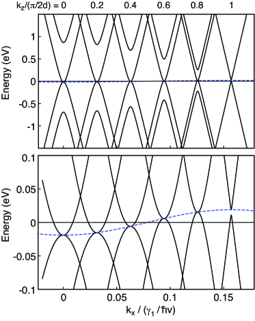
Figure 8: The band structure of AB-stacked bilayer graphene as a function of $k_{x}$ (with $k_{y}=0$). The subbands labeled by different $k_{z}$’s are separately plotted with horizontal shifts. The lower panel is the magnified plot of the same bands near zero energy. Blue dashed curves indicate the dispersion of the band touching point as a function of $k_{z}$.

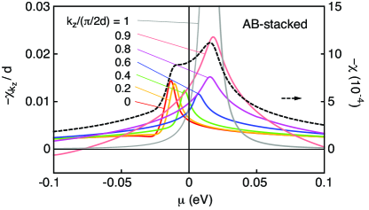
Figure 9: Magnetic susceptibility of AB-stacked graphite as a function of the chemical potential $\mu$, separately plotted for different $k_{z}$’s. The dashed curve is the total susceptibility.

For the magnetic susceptibility, we use the general expression based on the linear response theory,Fukuyama (1971)

$$\chi(\mu,T)=\int_{-\infty}^{\infty}d\epsilon f(\epsilon)\mbox{Im}F(\epsilon+i0),$$ (14)

with

$$F(z)=-\mu_{0}\frac{g_{v}g_{s}}{2\pi L^{3}}\frac{e^{2}}{\hbar^{2}}\sum_{\bf k}\mbox{tr}(G\mathcal{H}_{x}G\mathcal{H}_{y}G\mathcal{H}_{x}G\mathcal{H}_{y}).$$ (15)

Here $\mu$ is the chemical potential of electrons, $T$ is the temperature, $g_{v}=2$ and $g_{s}=2$ is the valley and spin degeneracy, respectively, $L$ is the system size, and $\mu_{0}$ is the vacuum permeability. We also defined $\mathcal{H}_{x}=\partial\mathcal{H}/\partial k_{x}$, $\mathcal{H}_{y}=\partial\mathcal{H}/\partial k_{y}$, $G(z)=(z-\mathcal{H})^{-1}$, and $f(\epsilon)=[1+e^{(\epsilon-\mu)/k_{B}T}]^{-1}$. The $\chi$ of this definition is the dimensionless susceptibility in the SI unit. The energy density of the magnetic field is given by $-\chi B^{2}/(2\mu_{0})$. By integration by parts in Eq.(14), we have

$$\chi(\mu,T)=\int_{-\infty}^{\infty}d\epsilon\left(-\frac{\partial f(\epsilon)}{\partial\epsilon}\right)\chi(\mu,T=0),$$ (16)

which relates the susceptibility at finite temperature with that at zero temperature. We include the energy broadening effect induced by the disorder potential by replacing $i0$ in Eq. (14) with a small self-energy $i\Gamma$ in the Green’s function. We assume the constant scattering rate $\Gamma=5$ meV in the following calculations.

Figure 9 plots the magnetic susceptibility of AB-stack graphite at fixed $k_{z}$’s (denoted as $\chi_{k_{z}}$) as a function of the chemical potential with the temperature $T=50$K, where the dashed curve is the total susceptibility $\chi=\int^{\pi/(2d)}_{-\pi/(2d)}\chi_{k_{z}}dk_{z}$. Approximately, $\chi_{k_{z}}$ is equivalent to that of bilayer graphene, which is a logarithmic peak centered at the band touching point and truncated at energies of $\pm\lambda(k_{z})\gamma_{1}$. Koshino and Ando (2007a, b) In increasing $k_{z}$, the peak becomes higher and it finally becomes a broadened delta function at the zone edge $k_{z}=\pi/(2d)$, which is an analog of the susceptibility of monolayer graphene. McClure (1956) The center of the peak moves as a function of $k_{z}$, in accordance with the shift of the band toughing point caused by $\gamma_{2}$ [Fig. 8]. We notice that the curves near $k_{z}=0$ has an additional sharp peak on top of the logarithmic background, which originates from the trigonal warping caused by $\gamma_{3}$. Koshino and Ando (2007a) The total susceptibility exhibits a broadened peak structure bound by $k_{z}=0$ peak and $k_{z}=\pi/(2d)$ peak, and its total width is of the order of $2\gamma_{2}\sim 0.04$eV.

Figure 3(a) shows the temperature dependence of the total susceptibility $\chi$ of AB-stacked graphite at $\mu=0$ (charge neutral). The temperature effect on the susceptibility can be understood by using Eq. (16), where $\chi(\mu)$ in a finite temperature is obtained by averaging $\chi(\mu)$ of zero temperature over an energy range of a few $k_{B}T$. In Fig.  3(a), $\chi$ logarithmically decreases as temperature increases, and this is understood as thermal broadening of the logarithmic peak of $\chi(\mu)$. When $k_{B}T$ is much smaller than the peak width of $\chi(\mu)$, the susceptibility does not depend much on the temperature, and this explains the nearly flat region in $T<50$ K in Fig. 3(a).

References

- Braunbek (1939) W. Braunbek, Zeitschrift für Physik 112, 764 (1939).
- Beaugnon and Tournier (1991) E. Beaugnon and R. Tournier, Nature 349, 470 (1991).
- Berry and Geim (1997) M. V. Berry and A. K. Geim, European Journal of Physics 18, 307 (1997).
- Simon and Geim (2000) M. Simon and A. Geim, Journal of applied physics 87, 6200 (2000).
- Winkleman et al. (2004) A. Winkleman, K. L. Gudiksen, D. Ryan, G. M. Whitesides, D. Greenfield, and M. Prentiss, Applied physics letters 85, 2411 (2004).
- McClure (1956) J. W. McClure, Phys. Rev. 104, 666 (1956).
- Fukuyama and Kubo (1970) H. Fukuyama and R. Kubo, J. Phys. Soc. Jpn. 28, 570 (1970).
- Sharma et al. (1974) M. Sharma, L. Johnson, and J. McClure, Physical Review B 9, 2467 (1974).
- Fukuyama (2007) H. Fukuyama, J. Phys. Soc. Jpn. 76, 043711 (2007).
- Koshino and Ando (2007a) M. Koshino and T. Ando, Phys. Rev. B 76, 085425 (2007a).
- Waldron (1966) R. D. Waldron, Review of Scientific Instruments 37, 29 (1966).
- Moser and Bleuler (2002) R. Moser and H. Bleuler, IEEE Transactions on applied superconductivity 12, 937 (2002).
- Moser et al. (2002) R. Moser, F. Barrot, J. Sandtner, and H. Bleuler, in 17th International Conference on Magnetically Levitated Systems and Linear Drives (Maglev) (2002).
- Boukallel et al. (2003) M. Boukallel, J. Abadie, and E. Piat, in 2003 IEEE International Conference on Robotics and Automation (Cat. No. 03CH37422), Vol. 3 (IEEE, 2003) pp. 3219–3224.
- Cansiz and Hull (2004) A. Cansiz and J. R. Hull, IEEE transactions on magnetics 40, 1636 (2004).
- Li et al. (2006) Q. Li, K.-S. Kim, and A. Rydberg, Review of scientific instruments 77, 065105 (2006).
- Liu et al. (2008) W. Liu, W.-Y. Chen, W.-P. Zhang, X.-G. Huang, and Z.-R. Zhang, Electronics Letters 44, 681 (2008).
- Mizutani et al. (2012) Y. Mizutani, A. Tsutsumi, T. Iwata, and Y. Otani, Journal of Applied Physics 111, 023909 (2012).
- Kustler (2012) G. Kustler, IEEE Transactions on Magnetics 48, 2044 (2012).
- Kobayashi and Abe (2012) M. Kobayashi and J. Abe, Journal of the American Chemical Society 134, 20593 (2012).
- Hilber and Jakoby (2013) W. Hilber and B. Jakoby, IEEE Sensors Journal 13, 2786 (2013).
- Su et al. (2015) Y. Su, Z. Xiao, Z. Ye, and K. Takahata, IEEE Electron Device Letters 36, 393 (2015).
- Kang et al. (2018) S. Kang, J. Kim, J.-B. Pyo, J. H. Cho, and T.-S. Kim, International Journal of Precision Engineering and Manufacturing-Green Technology 5, 341 (2018).
- Niu et al. (2018) C. Niu, F. Lin, Z. M. Wang, J. Bao, and J. Hu, Journal of Applied Physics 123, 044302 (2018).
- Ewall-Wice et al. (2019) M. Ewall-Wice, S. Yee, K. DeLawder, S. R. Montgomery, P. J. Joyce, C. Brownell, and H. ElBidweihy, IEEE Transactions on Magnetics (2019).
- Ominato and Koshino (2013) Y. Ominato and M. Koshino, Phys. Rev. B 87, 115433 (2013).
- Fukuyama (1971) H. Fukuyama, Prog. Theor. Phys. 45, 704 (1971).
- Wallace (1947) P. Wallace, Phys. Rev 71, 622 (1947).
- McClure (1957) J. W. McClure, Phys. Rev. 108, 612 (1957).
- Slonczewski and Weiss (1958) J. C. Slonczewski and P. R. Weiss, Phys. Rev. 109, 272 (1958).
- Dresselhaus and Dresselhaus (2002) M. S. Dresselhaus and G. Dresselhaus, Adv. Phys. 51, 1 (2002).
- Bistritzer and MacDonald (2011) R. Bistritzer and A. MacDonald, Proc. Natl. Acad. Sci. 108, 12233 (2011).
- de Laissardiere et al. (2012) G. T. de Laissardiere, D. Mayou, and L. Magaud, Phys. Rev. B 86, 125413 (2012).
- Camacho and Sosa (2013) J. Camacho and V. Sosa, Revista mexicana de física E 59, 8 (2013).
- Charlier et al. (1991) J.-C. Charlier, X. Gonze, and J.-P. Michenaud, Phys. Rev. B 43, 4579 (1991).
- Guinea et al. (2006) F. Guinea, A. Castro Neto, and N. Peres, Phys. Rev. B 73, 245426 (2006).
- Partoens and Peeters (2006) B. Partoens and F. Peeters, Phys. Rev. B 74, 075404 (2006).
- Guinea et al. (2007) F. Guinea, A. Castro Neto, and N. Peres, Solid state communications 143, 116 (2007).
- Koshino and Ando (2008) M. Koshino and T. Ando, Phys. Rev. B 77, 115313 (2008).
- McCann and Koshino (2013) E. McCann and M. Koshino, Reports on Progress in Physics 76, 056503 (2013).
- Koshino and Ando (2007b) M. Koshino and T. Ando, Phys. Rev. B 75, 235333 (2007b).