Structural Self-adaptation for Decentralized Pervasive Intelligence

Abstract

Communication structure plays a key role in the learning capability of decentralized systems. Structural self-adaptation, by means of self-organization, changes the order as well as the input information of the agents’ collective decision-making. This paper studies the role of agents’ repositioning on the same communication structure, i.e. a tree, as the means to expand the learning capacity in complex combinatorial optimization problems, for instance, load-balancing power demand to prevent blackouts or efficient utilization of bike sharing stations. The optimality of structural self-adaptations is rigorously studied by constructing a novel large-scale benchmark that consists of 4000 agents with synthetic and real-world data performing 4 million structural self-adaptations during which almost 320 billion learning messages are exchanged. Based on this benchmark dataset, 124 deterministic structural criteria, applied as learning meta-features, are systematically evaluated as well as two online structural self-adaptation strategies designed to expand learning capacity. Experimental evaluation identifies metrics that capture agents with influential information and their optimal positioning. Significant gain in learning performance is observed for the two strategies especially under low-performing initialization. Strikingly, the strategy that triggers structural self-adaptation in a more exploratory fashion is the most cost-effective.

I Introduction

The rise of distributed pervasive intelligence in the Internet of Things provides new unprecedented means to perform decentralized optimization and learning over communication networks [1]. Autonomous agents running on embedded devices can collaboratively solve complex optimization and learning problems without involvement of centralized third parties that do not scale, are single points of failure, require trust and privacy-sensitive data [2]. The critical role that structure plays in conventional machine learning algorithms has been earlier underlined, for instance, the number of layers in neural networks or the dropout of neurons to prevent over-fitting [3, 4]. However, little is known how communication structure influences decentralized learning in multi-agent systems.

This paper fills this gap by studying fixed and dynamic structural self-adaptations as the means of improving learning performance in challenging decentralized combinatorial optimization problems. Fixed adaptations concern deterministic criteria with which agents are repositioned within the same communication structure. This influences the order and the input information in agents’ collective decision-making. Dynamic adaptations concern a deterministic or random repositioning of agents during runtime to explore higher-performing solutions and escape from suboptimal trapped solutions. A novel methodology is introduced to study optimality of decentralized collective learning under structural self-adaptations. It relies on empirical data from real-world pilot projects for load-balancing power demand and bike sharing stations.

The contributions of this paper are outlined as follows: (i) A formal modeling approach of structural self-adaptation as a bijection of isomorphic graphs. (ii) A comparison of 124 structural self-adaptation criteria used as meta-features to improve offline or online learning performance. (iii) A modeling approach for designing online structural self-adaptations. (iv) Two customizable structural self-adaptation strategies to improve online learning performance. (v) A methodological approach to study the optimality of large-scale combinatorial optimization independent of data and application. (vi) An open benchmark dataset [5] of synthetic and real-world data for optimality evaluation. It contains 4 million performance profiles of structural self-adaptations generating almost 320 billion learning interactions among 4000 agents. (vii) Findings on the role of structural self-adaptations in learning aspects: optimality, application scenarios, network topology, self-adaptation parameters as well as computational and communication cost.

This paper is outlined as follows: Section II positions this work and Section III outlines related work. Section IV formalizes fixed and dynamic structural self-adaptations. Section V and VI discuss each of them respectively. Two online structural self-adaptation strategies are designed in Section VII. The experimental methodology is outlined in Section VIII and the experimental evaluation in Section IX. Finally, Section X concludes this paper and outlines future work.

II Research Positioning

This paper studies collective decision-making in multi-agent systems, in which agents have a set of discrete options to choose from. These options are resource consumption or production plans that are used for resource scheduling and allocation. For instance, a plan $\mathbf{p}$ can represent when a user charges its electric vehicle [6], the household energy demand over time, or the bike sharing stations from which a user picks up a bike or leaves one [2]. In practice, plans are sequences of real values. Each agent $a$ has multiple plans $\mathcal{P}_{a}$ that model the flexibility of the agent, its alternative options. Each agent may have preferences over its plans measured by a local cost assigned to each plan. For instance, the distance of a user from different bike sharing stations can measure the costs of plans.

An agent’s plan selection over the discrete planning options can satisfy local and global objectives, which can often be orthogonal to each other. Meeting local objectives is about choosing the plan with the lowest local cost, while global objectives concern the minimization of a global cost function with input the aggregate of all selected plans, i.e. element-wise summation. Agents can self-determine their preferences over the two objectives. On the one hand, linear cost functions can be minimized locally without coordinating the agents’ plan selections. For instance, minimizing the total power demand in the Smart Grid is a result of locally choosing the plan with the lowest power demand. On the other hand, minimization of quadratic cost functions, such as the minimization of variance, is a challenging non-convex combinatorial optimization problem that is NP-hard with complexity $O(k^{\mathsf{N}})$, where $k$ is the number of plans per agent and $\mathsf{N}$ is the total number of agents [7, 8, 2]. Coordination between the agents’ plan selections is required. The variance is used in this paper as a balancing indicator, e.g. lowering power peaks to prevent blackouts [9] or preserving a uniform number of bikes available at all bike sharing stations [2]. Methods that parallelize computations are one approach to solve such complex computational problems, for instance, BnB-ADOPT [10], NCBB [11] and DPOP [12]. However, such methods require universal access to agents’ information and therefore they are not designed for decentralized multi-agent systems preserving agents’ privacy and autonomy.

The alternative approach is to introduce a self-organzing communication structure that orchestrates in a cooperative and decentralized way searching of the combinatorial space [13]. This paper studies the role of such an agents’ structure in performance. It focuses on a certain structural self-adaptation that is the repositioning of the agents in a fixed topology as the means to explore the combinatorial solutions space. Agents’ positioning governs the input information from other agents based on which plan selections are made. In hierarchical structures such as trees, agents often interact in a bottom-up and top-down fashion [14]. The agents’ positioning governs the order of decision-making. A certain sequence of decision-making is a actually a coordination pattern: a traversal of the combinatorial solutions space. Different traversal strategies, i.e. criteria of agents’ positioning, may be trapped in different suboptimal solutions with different performance status.

It is fair to underline the challenge of determining causal relationships between performance and structure. Algorithmic artifacts introduce biases that are hard to distinguish from the role that the underlying structure plays. Given this challenge, this paper studies the decentralized collective learning system of I-EPOS, the Iterative Economic Planning and Optimized Selections [2, 15]. The interactive agents of I-EPOS self-organize in tree communication structures to coordinate plan selections. The exact mechanics of this coordination is subject of earlier work [2]. The structural self-adaptations studied in this paper are independent of I-EPOS that is used as a black box and a benchmark scenario given the following: (i) High efficiency as shown in comparisons with state of the art algorithms [2, 16, 17]. A high performance profile provides isolation of the performance analysis on structure, while inefficiencies by other algorithmic design choices are minimized. (ii) The core of the algorithm does not rely on exploration. Therefore the effect of structural self-adaptation as an exploration strategy can be easier isolated and studied.

III Related Work

There is evidence that structure plays a key role in exploration as certain topological properties support more effective communication and information diffussion [18]. Agents’ coordinated communication in reinforcement learning can be dynamically adapted to regulate learning performance and communication cost in distributed constraint optimization problems [19]. Similarly, performance of reinforcement learning can be improved by self-organizing agents into a supervisory network on top of an agents’ learning network. The latter is structured in dynamically formed groups via agents’ negotiation [20]. Structure may change as a result of network uncertainties such as network failures, latency and limited computational resources. Loss of learning performance as a result of such structural changes can be mitigated by localizing the learning process in part of a surviving network [21].

All aforementioned approaches involve (self-)organizational changes to improve learning performance, i.e. topological changes are performed. In contrast, this paper studies the agents’ relative repositioning over a fixed network and how it influences learning performance. Therefore, the scope of this paper has a more foundational character, while the findings illustrated are expected to provide new insights on the design of self-organization mechanisms for collective intelligence.

The agents’ positioning in a fixed learning structure can also be seen as an initialization problem of machine learning algorithms such as choosing the number of clusters and initial centroids in k-means that may result in slow convergence and empty clusters [22]. Bootstrapping solutions have been studied in this context [23]. Oscillating neural networks around optimal solutions may be a result of exploding gradients caused by high initializing weights [24, 25], instead of more random ones around zero [26]. It has also been shown that linearly non-separable data require hidden layers between input and output layers [27], while more than three hidden layers do not improve the learning performance of a feed-forward multi-layer perceptron [4]. Finally, adaptation of a neural network structure to the dimensionality of training data is critical to generalize and prevent over-fitting [3]. Applying these findings in the context of multi-agent systems and decentralized learning over networks with uncertainties is challenging and subject of ongoing research.

IV Structural Self-adaptation

Structural self-adaption is the repositioning of a set of agents $\mathcal{A}$ in a fixed tree topology and can be formalized as a bijection of isomorphic graphs:

Definition 1 (Bijection).

Let two tree graphs $\mathcal{G}$ and $\mathcal{H}$ having each a set of vertices $\mathcal{V}\left(\mathcal{G}\right)$, $\mathcal{V}\left(\mathcal{H}\right)$ and edges $\mathcal{E}\left(\mathcal{G}\right)$, $\mathcal{E}\left(\mathcal{H}\right)$ such that $\lvert\mathcal{V}\left(\mathcal{G}\right)\rvert=\lvert\mathcal{V}\left(\mathcal{H}\right)\rvert=\lvert\mathcal{A}\rvert=\mathsf{N}$ and $\lvert\mathcal{E}\left(\mathcal{G}\right)\rvert=\lvert\mathcal{E}\left(\mathcal{H}\right)\rvert=\mathsf{N}-1$. A bijection $b$ between the vertex sets of graphs $\mathcal{G}$ and $\mathcal{H}$ is defined as $b:\mathcal{V}\left(\mathcal{G}\right)\rightarrow\mathcal{V}\left(\mathcal{H}\right)$ such that two vertices $v$ and $w$ are adjacent in $\mathcal{G}$ if and only if vertices $b\left(v\right)$ and $b\left(w\right)$ are adjacent in $\mathcal{H}$.

Definition 2 (Isomorphism).

A graph $\mathcal{H}$ obtained by a bijection $b$ on graph $\mathcal{G}$ is an isomorphic graph to $\mathcal{G}\simeq\mathcal{H}$.

These definitions determine a fixed tree topology for the graphs $\mathcal{G}$ and $\mathcal{H}$, whose vertices host agents in different relative positions. There are $\lvert\mathcal{B}\rvert=\mathsf{N}!$ possible bijections, where $\mathcal{B}$ denotes all possible bijections on $\mathcal{G}$. Two bijection types are distinguished: (i) Fixed: These concern the agents’ positioning according to deterministic criteria. This paper reviews 124 criteria derived from metrics that measure features of the agents’ plans. They are used to sort agents in an ascending or descending order and position agents in the tree in a bottom-up breadth-first manner. Fixed bijections can be compared to show how different metrics with which sorting is performed influence learning performance. (ii) Dynamic: These concern the random or deterministic repositioning of the agents during learning runtime as the means to perform exploration of the solutions space so that learning performance improves by escaping from suboptimal trapped solutions. Four design elements model dynamic bijections and they are used to construct two online structural self-adaptation strategies.

In a decentralized environment in which each agent has a partial view of other agents, bijections of isomorphic tree graphs can be applied with two approaches: (i) migration and (ii) self-organization. Migration is the transfer of a piece of software and its state from one host to another. Migrations are earlier applied to multicasting trees and wireless sensor networks [28]. They have the advantage that no topological changes are required in the communication network, i.e. TCP connections are preserved. However, software migrations pose security challenges and may consume significant bandwidth resources. On the other hand, self-organization preserves the software locality, while the parent-child connections are adapted via a communication protocol. AETOS, the Adaptive Epidemic Tree Overlay Service is an example of such a self-organization mechanism [29]. Agents realize a bijection by interacting with each other to discover their new parent and children without any centralized mediating trusted party. A new pairing of two agents can be determined by their proximity e.g. Euclidean distance, between the ranking score of the two agents. The ranking score is calculated by deterministic metrics, i.e. Table I, or by a random score assignment, in case of an exploration. Decentralized building and maintenance of tree topologies has been extensively studied in earlier work with applications covering multimedia multicasting [30] and distributed databases [31]. In contrast, this paper focuses on (i) the impact of agents’ repositioning on the learning performance by self-organization as well as (ii) how repositioning can be triggered to improve learning performance. These challenges are not addressed in earlier work. They are the subject and contributions of this paper.

V Fixed Bijections

Fixed bijections are a subset of $\mathcal{B}$ and they are applied by executing the following steps: (1) Determine agents’ information based on which the ranking score is calculated. (2) Determine a metric to represent the agents’ information of Step 1. (3) Calculate the ranking score of each agent with the metric of Step 2. (4) Reposition and sort agents in a bottom-up breadth-first manner according to their ranking score.

In Step 1, agents may determine their ranking score based on the following: (i) the plans, (ii) the plan costs or (iii) their preferences on the global vs. local objective. This paper focuses on the plans to limit the number of studied dimensions.

Step 2 determines plan representations based on which isomorphic tree graphs are generated. Such representations are meta-features measuring deterministic plan characteristics. Table I introduces 62 metrics some of which include the following: minimum and maximum value of the possible plans, several correlation coefficients, metrics based on discrete sine and cosine transformations of the possible plans as well as metrics based on the Fourier transformation.

Table I: Reference list of structural self-adaptation metrics used as meta-features to improve learning performance. The mean operator $\mu_{\cdot}\left(\cdot\right)$ iterates over the subscript elements, while $\sigma(\cdot)$ indicates the standard deviation and $\times$ the Cartesian product.

Display Name	Full Name	Formula
avg-stdev	average standard deviation	$\mu_{\mathbf{p}\in\mathcal{P}_{a}}\left(\sigma\left(\mathbf{p}\right)\right)$
max-stdev	maximal standard deviation	$\underset{\mathbf{p}\in\mathcal{P}_{a}}{\max}{\sigma\left(\mathbf{p}\right)}$
min-stdev	minimal standard deviation	$\underset{\mathbf{p}\in\mathcal{P}_{a}}{\min}{\sigma\left(\mathbf{p}\right)}$
max-value	maximum value	$\underset{\mathbf{p}\in\mathcal{P}_{a},j=1,...,\mathsf{d}}{\max}\mathbf{p}_{j}$
min-value	minimum value	$\underset{\mathbf{p}\in\mathcal{P}_{a},j=1,...,\mathsf{d}}{\min}\mathbf{p}_{j}$
avg-corr-pearson	average Pearson coefficient	$\mu_{\mathbf{p}_{1},\mathbf{p}_{2}\in\mathcal{P}_{a}\times\mathcal{P}_{a}}\left(\mu_{j=1,...,\mathsf{d}}\left(corr_{p}\left(\mathbf{p}_{1},\mathbf{p}_{2}\right)_{j}\right)\right)$
avg-corr-kendall	average Kendall coefficient	$\mu_{\mathbf{p}_{1},\mathbf{p}_{2}\in\mathcal{P}_{a}\times\mathcal{P}_{a}}\left(\mu_{j=1,...,\mathsf{d}}\left(corr_{k}\left(\mathbf{p}_{1},\mathbf{p}_{2}\right)_{j}\right)\right)$
avg-corr-spearman	average Spearman coefficient	$\mu_{\mathbf{p}_{1},\mathbf{p}_{2}\in\mathcal{P}_{a}\times\mathcal{P}_{a}}\left(\mu_{j=1,...,\mathsf{d}}\left(corr_{s}\left(\mathbf{p}_{1},\mathbf{p}_{2}\right)_{j}\right)\right)$
max-avg-corr-pearson	max average Pearson coefficient	$\underset{\mathbf{p}_{1},\mathbf{p}_{2}\in\mathcal{P}_{a}\times\mathcal{P}_{a}}{\max}\mu_{j=1,...,\mathsf{d}}\left(corr_{p}\left(\mathbf{p}_{1},\mathbf{p}_{2}\right)_{j}\right)$
max-avg-corr-kendall	max average Kendall coefficient	$\underset{\mathbf{p}_{1},\mathbf{p}_{2}\in\mathcal{P}_{a}\times\mathcal{P}_{a}}{\max}\mu_{j=1,...,\mathsf{d}}\left(corr_{k}\left(\mathbf{p}_{1},\mathbf{p}_{2}\right)_{j}\right)$
max-avg-corr-spearman	max average Spearman coefficient	$\underset{\mathbf{p}_{1},\mathbf{p}_{2}\in\mathcal{P}_{a}\times\mathcal{P}_{a}}{\max}\mu_{j=1,...,\mathsf{d}}\left(corr_{s}\left(\mathbf{p}_{1},\mathbf{p}_{2}\right)_{j}\right)$
min-avg-corr-pearson	min average Pearson coefficient	$\underset{\mathbf{p}_{1},\mathbf{p}_{2}\in\mathcal{P}_{a}\times\mathcal{P}_{a}}{\min}\mu_{j=1,...,\mathsf{d}}\left(corr_{p}\left(\mathbf{p}_{1},\mathbf{p}_{2}\right)_{j}\right)$
min-avg-corr-kendall	min average Kendall coefficient	$\underset{\mathbf{p}_{1},\mathbf{p}_{2}\in\mathcal{P}_{a}\times\mathcal{P}_{a}}{\min}\mu_{j=1,...,\mathsf{d}}\left(corr_{k}\left(\mathbf{p}_{1},\mathbf{p}_{2}\right)_{j}\right)$
min-avg-corr-spearman	min average Spearman coefficient	$\underset{\mathbf{p}_{1},\mathbf{p}_{2}\in\mathcal{P}_{a}\times\mathcal{P}_{a}}{\min}\mu_{j=1,...,\mathsf{d}}\left(corr_{s}\left(\mathbf{p}_{1},\mathbf{p}_{2}\right)_{j}\right)$
avg-max-corr-pearson	average max Pearson coefficient	$\mu_{\mathbf{p}_{1},\mathbf{p}_{2}\in\mathcal{P}_{a}\times\mathcal{P}_{a}}\left(\underset{j=1,...,\mathsf{d}}{\max}\quad corr_{p}\left(\mathbf{p}_{1},\mathbf{p}_{2}\right)_{j}\right)$
avg-max-corr-kendall	average max Kendall coefficient	$\mu_{\mathbf{p}_{1},\mathbf{p}_{2}\in\mathcal{P}_{a}\times\mathcal{P}_{a}}\left(\underset{j=1,...,\mathsf{d}}{\max}\quad corr_{k}\left(\mathbf{p}_{1},\mathbf{p}_{2}\right)_{j}\right)$
avg-max-corr-spearman	average max Spearman coefficient	$\mu_{\mathbf{p}_{1},\mathbf{p}_{2}\in\mathcal{P}_{a}\times\mathcal{P}_{a}}\left(\underset{j=1,...,\mathsf{d}}{\max}\quad corr_{s}\left(\mathbf{p}_{1},\mathbf{p}_{2}\right)_{j}\right)$
avg-min-corr-pearson	average min Pearson coefficient	$\mu_{\mathbf{p}_{1},\mathbf{p}_{2}\in\mathcal{P}_{a}\times\mathcal{P}_{a}}\left(\underset{j=1,...,\mathsf{d}}{\min}\quad corr_{p}\left(\mathbf{p}_{1},\mathbf{p}_{2}\right)_{j}\right)$
avg-min-corr-kendall	average min Kendall coefficient	$\mu_{\mathbf{p}_{1},\mathbf{p}_{2}\in\mathcal{P}_{a}\times\mathcal{P}_{a}}\left(\underset{j=1,...,\mathsf{d}}{\min}\quad corr_{k}\left(\mathbf{p}_{1},\mathbf{p}_{2}\right)_{j}\right)$
avg-min-corr-spearman	average min Spearman coefficient	$\mu_{\mathbf{p}_{1},\mathbf{p}_{2}\in\mathcal{P}_{a}\times\mathcal{P}_{a}}\left(\underset{j=1,...,\mathsf{d}}{\min}\quad corr_{s}\left(\mathbf{p}_{1},\mathbf{p}_{2}\right)_{j}\right)$
max-corr-pearson	max Pearson coefficient	$\underset{\mathbf{p}_{1},\mathbf{p}_{2}\in\mathcal{P}_{a}\times\mathcal{P}_{a}}{\max}{\underset{j=1,...,\mathsf{d}}{\min}\quad corr_{p}\left(\mathbf{p}_{1},\mathbf{p}_{2}\right)_{j}}$
max-corr-kendall	max Kendall coefficient	$\underset{\mathbf{p}_{1},\mathbf{p}_{2}\in\mathcal{P}_{a}\times\mathcal{P}_{a}}{\max}{\underset{j=1,...,\mathsf{d}}{\min}\quad corr_{k}\left(\mathbf{p}_{1},\mathbf{p}_{2}\right)_{j}}$
max-corr-spearman	max Spearman coefficient	$\underset{\mathbf{p}_{1},\mathbf{p}_{2}\in\mathcal{P}_{a}\times\mathcal{P}_{a}}{\max}{\underset{j=1,...,\mathsf{d}}{\min}\quad corr_{s}\left(\mathbf{p}_{1},\mathbf{p}_{2}\right)_{j}}$
min-corr-pearson	min Pearson coefficient	$\underset{\mathbf{p}_{1},\mathbf{p}_{2}\in\mathcal{P}_{a}\times\mathcal{P}_{a}}{\min}{\underset{j=1,...,\mathsf{d}}{\min}\quad corr_{p}\left(\mathbf{p}_{1},\mathbf{p}_{2}\right)_{j}}$
min-corr-kendall	min Kendall coefficient	$\underset{\mathbf{p}_{1},\mathbf{p}_{2}\in\mathcal{P}_{a}\times\mathcal{P}_{a}}{\min}{\underset{j=1,...,\mathsf{d}}{\min}\quad corr_{k}\left(\mathbf{p}_{1},\mathbf{p}_{2}\right)_{j}}$
min-corr-spearman	min Spearman coefficient	$\underset{\mathbf{p}_{1},\mathbf{p}_{2}\in\mathcal{P}_{a}\times\mathcal{P}_{a}}{\min}{\underset{j=1,...,\mathsf{d}}{\min}\quad corr_{s}\left(\mathbf{p}_{1},\mathbf{p}_{2}\right)_{j}}$
avg-dct1-coeff	average DCT 1 coefficient	$\mu_{\mathbf{p}\in\mathcal{P}_{a}}\left(\mu_{j=1,...,\mathsf{d}}\left(dct_{1}\left(\mathbf{p}\right)_{j}\right)\right)$
avg-dct2-coeff	average DCT 2 coefficient	$\mu_{\mathbf{p}\in\mathcal{P}_{a}}\left(\mu_{j=1,...,\mathsf{d}}\left(dct_{2}\left(\mathbf{p}\right)_{j}\right)\right)$
avg-dct3-coeff	average DCT 3 coefficient	$\mu_{\mathbf{p}\in\mathcal{P}_{a}}\left(\mu_{j=1,...,\mathsf{d}}\left(dct_{3}\left(\mathbf{p}\right)_{j}\right)\right)$
max-dct1-coeff	max DCT 1 coefficient	$\underset{\mathbf{p}\in\mathcal{P}_{a}}{\max}\quad\underset{j=1,...,\mathsf{d}}{\max}\quad dct_{1}\left(\mathbf{p}\right)_{j}$

Display Name	Full Name	Formula
max-dct2-coeff	max DCT 2 coefficient	$\underset{\mathbf{p}\in\mathcal{P}_{a}}{\max}\quad\underset{j=1,...,\mathsf{d}}{\max}\quad dct_{2}\left(\mathbf{p}\right)_{j}$
max-dct3-coeff	max DCT 3 coefficient	$\underset{\mathbf{p}\in\mathcal{P}_{a}}{\max}\quad\underset{j=1,...,\mathsf{d}}{\max}\quad dct_{3}\left(\mathbf{p}\right)_{j}$
min-dct1-coeff	min DCT 1 coefficient	$\underset{\mathbf{p}\in\mathcal{P}_{a}}{\min}\quad\underset{j=1,...,\mathsf{d}}{\min}\quad dct_{1}\left(\mathbf{p}\right)_{j}$
min-dct2-coeff	min DCT 2 coefficient	$\underset{\mathbf{p}\in\mathcal{P}_{a}}{\min}\quad\underset{j=1,...,\mathsf{d}}{\min}\quad dct_{2}\left(\mathbf{p}\right)_{j}$
min-dct3-coeff	min DCT 3 coefficient	$\underset{\mathbf{p}\in\mathcal{P}_{a}}{\min}\quad\underset{j=1,...,\mathsf{d}}{\min}\quad dct_{3}\left(\mathbf{p}\right)_{j}$
avg-max-dct1-coeff	average max DCT 1 coefficient	$\mu_{\mathbf{p}\in\mathcal{P}_{a}}\left(\underset{j=1,...,\mathsf{d}}{\max}\quad dct_{1}\left(\mathbf{p}\right)_{j}\right)$
avg-max-dct2-coeff	average max DCT 2 coefficient	$\mu_{\mathbf{p}\in\mathcal{P}_{a}}\left(\underset{j=1,...,\mathsf{d}}{\max}\quad dct_{2}\left(\mathbf{p}\right)_{j}\right)$
avg-max-dct3-coeff	average max DCT 3 coefficient	$\mu_{\mathbf{p}\in\mathcal{P}_{a}}\left(\underset{j=1,...,\mathsf{d}}{\max}\quad dct_{3}\left(\mathbf{p}\right)_{j}\right)$
avg-min-dct1-coeff	average min DCT 1 coefficient	$\mu_{\mathbf{p}\in\mathcal{P}_{a}}\left(\underset{j=1,...,\mathsf{d}}{\min}\quad dct_{1}\left(\mathbf{p}\right)_{j}\right)$
avg-min-dct2-coeff	average min DCT 2 coefficient	$\mu_{\mathbf{p}\in\mathcal{P}_{a}}\left(\underset{j=1,...,\mathsf{d}}{\min}\quad dct_{2}\left(\mathbf{p}\right)_{j}\right)$
avg-min-dct3-coeff	average min DCT 3 coefficient	$\mu_{\mathbf{p}\in\mathcal{P}_{a}}\left(\underset{j=1,...,\mathsf{d}}{\min}\quad dct_{3}\left(\mathbf{p}\right)_{j}\right)$
avg-dst1-coeff	average DST 1 coefficient	$\mu_{\mathbf{p}\in\mathcal{P}_{a}}\left(\mu_{j=1,...,\mathsf{d}}\left(dst_{1}\left(\mathbf{p}\right)_{j}\right)\right)$
avg-dst2-coeff	average DST 2 coefficient	$\mu_{\mathbf{p}\in\mathcal{P}_{a}}\left(\mu_{j=1,...,\mathsf{d}}\left(dst_{2}\left(\mathbf{p}\right)_{j}\right)\right)$
avg-dst3-coeff	average DST 3 coefficient	$\mu_{\mathbf{p}\in\mathcal{P}_{a}}\left(\mu_{j=1,...,\mathsf{d}}\left(dst_{3}\left(\mathbf{p}\right)_{j}\right)\right)$
max-dst1-coeff	max DST 1 coefficient	$\underset{\mathbf{p}\in\mathcal{P}_{a}}{\max}\quad\underset{j=1,...,\mathsf{d}}{\max}\quad dst_{1}\left(\mathbf{p}\right)_{j}$
max-dst2-coeff	max DST 2 coefficient	$\underset{\mathbf{p}\in\mathcal{P}_{a}}{\max}\quad\underset{j=1,...,\mathsf{d}}{\max}\quad dst_{2}\left(\mathbf{p}\right)_{j}$
max-dst3-coeff	max DST 3 coefficient	$\underset{\mathbf{p}\in\mathcal{P}_{a}}{\max}\quad\underset{j=1,...,\mathsf{d}}{\max}\quad dst_{3}\left(\mathbf{p}\right)_{j}$
min-dst1-coeff	min DST 1 coefficient	$\underset{\mathbf{p}\in\mathcal{P}_{a}}{\min}\quad\underset{j=1,...,\mathsf{d}}{\min}\quad dst_{1}\left(\mathbf{p}\right)_{j}$
min-dst2-coeff	min DST 2 coefficient	$\underset{\mathbf{p}\in\mathcal{P}_{a}}{\min}\quad\underset{j=1,...,\mathsf{d}}{\min}\quad dst_{2}\left(\mathbf{p}\right)_{j}$
min-dst3-coeff	min DST 3 coefficient	$\underset{\mathbf{p}\in\mathcal{P}_{a}}{\min}\quad\underset{j=1,...,\mathsf{d}}{\min}\quad dst_{3}\left(\mathbf{p}\right)_{j}$
avg-max-dst1-coeff	average max DST 1 coefficient	$\mu_{\mathbf{p}\in\mathcal{P}_{a}}\left(\underset{j=1,...,\mathsf{d}}{\max}\quad dst_{1}\left(\mathbf{p}\right)_{j}\right)$
avg-max-dst2-coeff	average max DST 2 coefficient	$\mu_{\mathbf{p}\in\mathcal{P}_{a}}\left(\underset{j=1,...,\mathsf{d}}{\max}\quad dst_{2}\left(\mathbf{p}\right)_{j}\right)$
avg-max-dst3-coeff	average max DST 3 coefficient	$\mu_{\mathbf{p}\in\mathcal{P}_{a}}\left(\underset{j=1,...,\mathsf{d}}{\max}\quad dst_{3}\left(\mathbf{p}\right)_{j}\right)$
avg-min-dst1-coeff	average min DST 1 coefficient	$\mu_{\mathbf{p}\in\mathcal{P}_{a}}\left(\underset{j=1,...,\mathsf{d}}{\min}\quad dst_{1}\left(\mathbf{p}\right)_{j}\right)$
avg-min-dst2-coeff	average min DST 2 coefficient	$\mu_{\mathbf{p}\in\mathcal{P}_{a}}\left(\underset{j=1,...,\mathsf{d}}{\min}\quad dst_{2}\left(\mathbf{p}\right)_{j}\right)$
avg-min-dst3-coeff	average min DST 3 coefficient	$\mu_{\mathbf{p}\in\mathcal{P}_{a}}\left(\underset{j=1,...,\mathsf{d}}{\min}\quad dst_{3}\left(\mathbf{p}\right)_{j}\right)$
sum-of-0-dft-coeff	sum of $0^{th}$ DFT coefficient	$\left\lvert\sum_{\mathbf{p}\in\mathcal{P}_{a}}\mathcal{F}\left(\mathbf{p}\right)_{0}\right\rvert$
max-of-0-dft-coeff	max of $0^{th}$ DFT coefficient	$\left\lvert\underset{\mathbf{p}\in\mathcal{P}_{a}}{\max}\quad\mathcal{F}\left(\mathbf{p}\right)_{0}\right\rvert$
sum-non0-dft-coeff	sum of non-$0^{th}$ DFT coefficient	$\left\lvert\sum_{\mathbf{p}\in\mathcal{P}_{a}}\sum_{j=1,...,\mathsf{d}}\mathcal{F}\left(\mathbf{p}\right)_{j}\right\rvert$
max-non0-dft-coeff	max of non-$0^{th}$ DFT coefficient	$\left\lvert\underset{\mathbf{p}\in\mathcal{P}_{a}}{\max}\quad\underset{j=1,...,\mathsf{d}}{\max}\quad\mathcal{F}\left(\mathbf{p}\right)_{j}\right\rvert$
sum-all-dft-coeff	sum of DFT coefficient	$\left\lvert\sum_{\mathbf{p}\in\mathcal{P}_{a}}\sum_{j=1,...,\mathsf{d}}\mathcal{F}\left(\mathbf{p}\right)_{j}\right\rvert$
avg-stdev-dft-coeff	average std dev of DFT coefficients	$\left\lvert\mu_{\mathbf{p}\in\mathcal{P}_{a}}\left(\sigma\left(\mathcal{F}\left(\mathbf{p}\right)\right)\right)\right\rvert$

Next in Step 3, agents use the selected metrics to calculate their ranking score with which a proximity between agent pairs can be determined, e.g. Euclidean distance.

Finally, in Step 4, self-organization mechanisms, such as AETOS [29], use the agents’ proximity information to reposition agents on the same balanced tree by sorting them in a bottom-up breadth-first manner as shown in Figure 1. Agents can be positioned in both ascending and descending order.

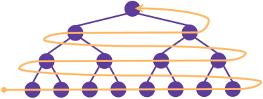
Figure 1: Bottom-up, breadth-first in a balanced tree.

To incept the impact of fixed bijections on learning performance consider a sequence of consecutive agents’ decisions that progresses from the leaves up to the root. Each agent that performs its plan selection coordinates with the other agents underneath, i.e. takes into account the aggregate selected plans of these agents. Assume an agent with highly influential plans in the sense that when these plans aggregate with the plans of other agents, the global cost explodes. This can be because of plans with extreme oscillations or plans, whose mean value is significantly higher than the one of the other agents. The closer to the root this agent with the influential plans is, the lower the likelihood to adjust the aggregate selections of the agents underneath. This is because the number of the remaining agents above decreases and the remaining plan selections may not be enough to lower down the global cost. Therefore, learning performance can potentially improve if this agent is positioned at the bottom part of the tree to preserve a higher number of agents above to compensate and eventually drop down the global cost.

VI Dynamic Bijections

A structural self-adaptation via a bijection initializes a new learning phase in which learning performance improves further. Four design elements are introduced to model strategies for structural self-adaptations: (i) A mechanism to realize a bijection. (ii) A memory scheme of solutions for initializing the next learning phase. (iii) A criterion to trigger structural self-adaptation. (iv) A bijection type to apply.

VI-A Realizing a bijection

Agents can realize themselves a structural self-adaptation without relying on a trusted third party. Assuming agents can execute a migration [28] or self-organization service such as AETOS [29], this execution can be independently triggered by each I-EPOS agent based on system-wide criteria. For instance, the global cost, i.e. variance, is calculated using the final aggregate plan propagated during the top-down phase of each learning iteration. This approach assumes common criteria for all agents, otherwise agents need to reach consensus of when to perform the bijection. Such consensus can be reached via, for instance, voting mechanisms, which are broadly used in distributed ledgers and blockchain technologies [32].

A migration or self-organization service can also been seen as a black box: Each agent provides as input its ranking score as well as its current children and parent, while it receives as output the respective new ones. Aggregate plans become outdated by establishing a new structure. Descendants change and the learning process requires reinitialization. Nevertheless, the selected plans at an earlier learning phase remain valid and represent a (good) found solution. Therefore, the learning process with the new agents’ positioning can be initialized with these plans, instead of default random ones, to explore whether this previous solution can be further improved while preventing performance degradation. Structural self-adaptation can be triggered multiple times to explore the solution space until one or more conditions are met, e.g. the global cost is lower than some threshold or until a maximal number of learning iterations is performed.

VI-B Reinitialization via short-term vs. long-term memory

After structural self-adaptation, a new learning process is initialized with selected plans from the earlier learning phase. A (i) short-term and (ii) long-term memory scheme are introduced that assume limited resources: memory is bounded to the storage of a single earlier selected plan.

Short-term memory restores the selected plans from the last iteration of the earlier learning phase. Long term memory restores the selected plans from an iteration of the earlier phase determined by a fixed memory offset. This offset is the learning iteration on which the selected plans are memorized. For instance, agents with an offset of 3, memorize the selected plans at the $3^{rd}$ iteration, which are restored at iteration $0$ of the next learning phase. An offset equals to the convergence iteration is equivalent to short-term memory. Different offset values are studied in this paper provided as learning parameters.

While short-term memory memorizes the selected plans of a suboptimal trapped solution found on convergence, long-term memory sacrifices learning performance as the means to escape from this trapped solution and potentially discover a better performing one at the next learning phase. Between consecutive learning phases with offset $>0$, the global cost is monotonically non-increasing: at least as low as the one of the offset iteration during the previous learning phase.

VI-C Criteria to trigger structural self-adaptation

Two criteria for triggering structural self-adaptation are introduced: (i) convergence and (ii) global cost reduction.

The convergence criterion triggers structural self-adaptation when convergence is reached, i.e. when the global cost in two consecutive iterations remains the same. The criterion of global cost reduction triggers a structural self-adaptation when global cost drops below a certain threshold, provided as system parameter. This threshold represents a sufficient decrease of the global cost measured by the slope. The higher the slope, the higher the global cost reduction. Consequently, larger reduction steps are still in progress and further learning iterations are required for convergence. On the contrary, when the slope is low, global cost reduction decreases and as a result learning approaches convergence. The slope is measured by the relative difference between the global cost $G^{\left(t\right)}$ and $G^{\left(t-1\right)}$ of two consecutive learning iterations $t$ and $t-1$: $s=\frac{G^{\left(t-1\right)}-G^{\left(t\right)}}{G^{\left(t-1\right)}}$. The absolute difference between the global costs at two consecutive iterations $w=G^{\left(t-1\right)}-G^{\left(t\right)}$ is referred to as a residual. The slope and the respective threshold receive values in the range $[0,1]$. A threshold value of 0 prohibits structural self-adaptation, while a value of 1 forces such self-adaptation every two iterations, given that a current and a previous iterations are required to compute a residual.

VI-D Bijection types

Two bijection types are distinguished: (i) deterministic and (ii) random. Deterministic bijections are the ones generated with metrics such as the ones of Table I. These metrics calculate the ranking score of the agents based on which sorting is performed. Determining the effectiveness of deterministic bijections in online structural self-adaptations is not straightforward as it highly depends on the memory scheme employed as well as the shape of the combinatorial landscape, i.e. the plans and their cost. Therefore, offline deterministic bijections are studied to understand their primitive role on learning performance before moving to an online context that is subject of future work. Random bijections are generated by assigning a random ranking score to each agent. Based on this random score, the self-organization service returns a repositioning of the agents, a bijection $b\in\mathcal{B}$. Random bijections are used during the learning runtime as an exploratory strategy to escape from suboptimum trapped solutions.

VII Online Structural Self-adaptation

Figure 2 introduces two online structural self-adaptation strategies based on dynamic bijections.

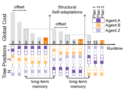
(a) Convergence criterion with long-term memory.

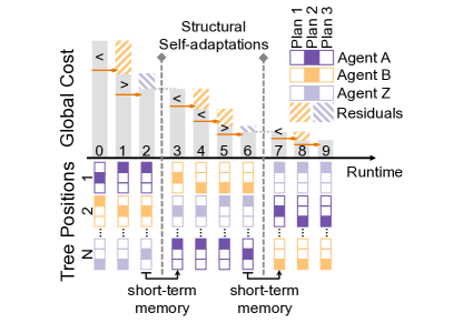
(b) Global cost criterion with short-term memory.

Figure 2: The two online structural self-adaptation strategies.

Figure 2a illustrates the strategy based on the convergence criterion with long-term memory. It is shown for an offset of $2$. Convergence is detected on the 5th iteration triggering structural self-adaptation. The new learning phase begins on the $6^{th}$ iteration initialized by the selected plans of the $2^{nd}$ iteration as indicated by the vertical dotted line. The process repeats until the $13{th}$ iteration when the algorithm terminates. The termination condition is the detection of convergence before reaching the offset iteration.

Figure 2b shows the strategy based on the global cost reduction criterion with short-term memory. A threshold of 25% is marked by horizontal pointers between the bars of two consecutive iterations. The residual on the 1st iteration is higher than the 25% threshold that prevents self-adaptation. The slope drops below threshold on the $2^{nd}$ iteration triggering self-adaptation. The new learning phase is initialized on the $3^{rd}$ iteration with the selected plans of the $2^{nd}$ iteration indicated by the vertical dotted line. Note the preservation of the global cost reduction. The strategy criterion is met next on the $6^{th}$ iteration. Termination is detected on the $9^{th}$ iteration when no change in the slope is observed.

VIII Experimantal Methodology

This section introduces the evaluation methodology of fixed and dynamic bijections. The employed synthetic and real-world datasets are discussed, followed by the parameterization of I-EPOS and the studied variables, i.e. number of children. A novel evaluation methodology is introduced for assessing the optimality of the solutions independent of the employed dataset. This methodology allows the systematic evaluation of the online strategies for structural self-adaptation.

VIII-A Synthetic and real-world datasets

Table II outlines the datasets [33] and the main experimental settings. A synthetic dataset with plan values drawn from a Normal distribution is used as well as two real-world datasets from pilot projects [2]: (i) Energy–This dataset is a disaggregation result of the zonal power transmission system in the Pacific Northwest Smart Grid demonstration project [34]. The first plan is the original disaggregated load. The following three plans are computed by the SHUFFLE plan generation scheme that randomly shuffles the values of the first plan. The next three plans are computed by the SWAP-15 generation scheme that randomly selects 15 pairs of values to swap. The final three plans are generated respectively via SWAP-30. Consequently, the mean and the standard deviation of all possible plans are equal for each agent. (ii) Bicycle–This dataset consists of the trip records of the Hubway bike sharing system in Paris [2]. Trips match to users via the data fields of zip code, year of birth and gender. Each plan value measures the difference in the number of incoming and outgoing trips at a bike station. For example, if a user cycled between stations 1 and 3, the corresponding possible plan is $\{-1,0,1,0,...\}$. Different trips of a user are encoded as different possible plans.

Table II: An outline of the datasets and experimental settings.

Parameter		Datasets [33]
		Bicycle	Energy	Synthetic
Global cost function		minimization of variance
Tree type		default: binary $\mathcal{H}_{b},\quad\forall b\in\mathcal{S}$
Number of agents		$\mathsf{N}=1000$	$\mathsf{N}=1000$	$\mathsf{N}=1000$
Number of plans		$\lvert\mathcal{P}_{a}\rvert\leq 23,\forall a\in\mathcal{A}$	$\lvert\mathcal{P}_{a}\rvert=10,\forall a\in\mathcal{A}$	$\lvert\mathcal{P}_{a}\rvert=16,\forall a\in\mathcal{A}$
Dimension of plans		$\mathsf{d}=98$	$\mathsf{d}=144$	$\mathsf{d}=100$
Number of iterations		$T=40$	$T=40$	$T=40$

VIII-B Collective learning parameterization

I-EPOS runs by default on a binary balanced tree. A varied number of children, from 2 to 14, is evaluated for fixed bijections. A higher number of children for each agent results in more informed plan selections, however, the number of leaves that make plan selections without information from descendants increases: for a balanced binary tree with 1000 agents, the number of leaves is 500 (50%), whereas for a 14-ary balanced tree, the number of leaves is 928 (92.8%). I-EPOS minimizes the global cost function that is the variance used as a balancing criterion: reducing the power peaks and load-balancing the utilization of the bike sharing stations. To stretch the collective learning performance, only the global cost function is optimized and therefore the I-EPOS parameter of $\lambda=0$ ignores the local cost function.

VIII-C Evaluation approach for optimality

The empirical evaluation of optimality concerns the ranking of the found solution in terms of global cost out of all possible solutions in the combinatorial space that is $k^{\mathsf{N}}$. As the scale of the combinatorial space explodes for a high number of plans and agents, such an evaluation is particularly challenging. Earlier work limits the optimality evaluation to a low number of agents and plans per agent, e.g. $k^{\mathsf{N}}=2^{20}=4^{10}$ [2]. This paper contributes an alternative approach that constructs a representative sample of potentially high-performing solutions using I-EPOS operating with random bijections applied on isomorphic tree graphs. This approach has the following advantages: (i) A profiling of high-performing solutions for different datasets using the same learning methodology, I-EPOS, without employing other heuristics or brute-force. (ii) An efficient computation of a large number of random bijections and their learning performance is feasible and can be performed offline using parallel batch processing.

A benchmark dataset is generated using the aforementioned approach with both deterministic and random bijections applied to I-EPOS. This dataset [5] is a contribution of this paper and it can be used to encourage and support further research on combinatorial optimization and learning. A total of 1 million ($\lvert\mathcal{S}\rvert=10^{6}$) random bijections are generated for each dataset. I-EPOS runs for 40 iterations with each of these bijections. In total, $10^{6}$ bijections $\ast$ $4$ datasets $\ast$ $40$ iterations $\ast$ $(1000-1)$ $\ast$ $2$ messages per iteration calculate the total of $\approx 320$ billion learning messages. I-EPOS instances run in parallel in their own Java virtual machine on a Hetzner dedicated server.

The performance profiling of the solutions discovered via random bijections depends on the application, i.e. the data values of the plans. The ranking of the solutions, according to global cost, can be generalized by calculating instead the percentile in which a solution is found. This method assumes a common distribution of the global cost among the different datasets. To test this assumption, the global cost is modeled as a random variable $\mathcal{X}$ that has unknown distribution but is dependent on the random bijections $\mathcal{B}$.

At first the probability density function of $\mathcal{X}$ is estimated in a non-parametric way using the kernel density estimation fed with the global cost of I-EPOS for all isomorphic graphs of $\mathcal{S}$. A Gaussian kernel is used with a bandwidth suggested in earlier work [35]: $n^{-\frac{1}{5}}$, which is equal to $0.0631$ for $n=10^{6}$.

Next the global cost as a random variable $\mathcal{X}$ is modeled by a Gaussian distribution with unknown expectation and variance that are estimated using the mean ($50^{th}$ percentile) and variance of the global costs from the benchmark dataset.

If the non-parametric kernel density estimation matches the parametric one, the learning performance based on percentiles can be reliably compared among the different datasets. With this methodology, the optimality of deterministic bijections can be rigorously studied by generalizing and linking their performance profile to the performance percentiles of random bijections. For each of the 62 metrics of Table I, two bijections are applied, each of them sorts agents in ascending and descending order. From the total of 124 fixed bijections, 39 of them are selected for illustration in this paper.

VIII-D Evaluation approach for self-adaptation strategies

For the evaluation of the two structural self-adaptation strategies, I-EPOS is initialized with three random isomorphic tree networks corresponding to the $10^{th}$, $50^{th}$ and $90^{th}$ percentile referred to as baselines, while a structural self-adaptation is triggered with a sample of an isomorphic tree graph from the whole set $\mathcal{B}$. Due to the random sampling involved, the execution of the two strategies repeats 100 times. Their learning performance is evaluated with the average relative improvement in the global cost reduction between the baselines and the strategies over all repetitions. A positive relative improvement results in higher learning performance by the strategies compared to the baselines, while a negative one results in a lower learning performance respectively. The memory offset and the threshold for each of the two strategies vary in the range $[1,20]$ and $[0.1,0.9]$ respectively, with a step $0.1$ for the latter. The total learning runtime is 100 iterations during which structural self-adaptations are performed.

Controlling the number of structural self-adaptations is critical for the cost-effectiveness of learning. Repositioning agents requires communication and computational cost, e.g. AETOS introduces interactions between agents to discover and connect the parent and child with the closest proximity [29]. The two strategies are also compared in terms of the number of self-adaptation they perform until termination.

IX Experimantal Evaluation

This section validates the methodology for assessing learning optimality with isomorphic tree graphs followed by the evaluation of fixed and dynamic bijections.

IX-A Learning optimality with isomorphic tree graphs

The one million isomorphic graphs are sorted from high to low according to the global cost at convergence for each dataset and are shown in Figure 3a, 3b and 3c. The following observations can be made: (i) The shape of all sorted solutions is similar among datasets, i.e. very few solutions at extremes while the majority decreases linearly. (ii) The solutions shape resembles the ones obtained for small-scale networks via brute-force as shown in Figure 21 and 22 of earlier work [2]. (iii) There is accurate correspondence of the percentiles among the different datasets. (iv) The global cost reduction compared to the maximal observed value is 58.6%, 71.2%, 65.07% for the synthetic, energy and bicycle dataset respectively.

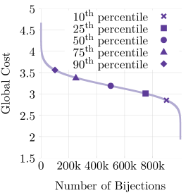
(a) Synthetic dataset

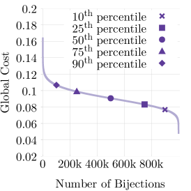
(b) Energy dataset

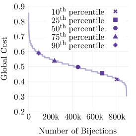
(c) Bicycle dataset

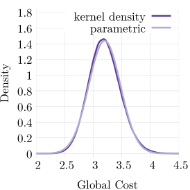
(d) synthetic dataset

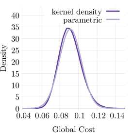
(e) Energy dataset

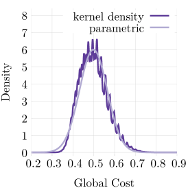
(f) Bicycle dataset

Figure 3: Performance profiling of $10^{6}$ random bijections.

The parametric and non-parametric global cost distributions obtained with random isomorphic graphs are compared in Figure 3d, 3e and 3f for each dataset.

The expectation and variance of the parametric Gaussian distribution are estimated using the benchmark dataset constructed as follows: $\mathcal{X}_{\text{s}}\sim\mathcal{N}\left(\mu=3.1989,\sigma^{2}=0.0771\right)$, $\mathcal{X}_{\text{e}}\sim\mathcal{N}\left(\mu=0.0913,\sigma^{2}=0.0001\right)$ and $\mathcal{X}_{\text{b}}\sim\mathcal{N}\left(\mu=0.4981,\sigma^{2}=0.0044\right)$ for the synthetic, energy and bicycle dataset respectively. The kernel density estimator approximates very closely the parametric densities in all three datasets without making any assumptions about the underlying data and therefore it holds that $\mathcal{X}\sim\mathcal{N}\left(\mu,\sigma^{2}\right)$.

IX-B Learning performance with fixed bijections

Figure 4 illustrates the learning performance of the 39 selected metrics, listed in an ascending order. Note that metrics such as ASC-min-corr-pearson or ASC-min-dst1-coeff have high performance in all three datasets and they are likely to capture fundamental structural characteristics influencing collective learning. The metric DESC-min-value reaches the $25^{th}$ percentile, while its ascending version reaches the $51^{st}$ percentile. This confirms the earlier intuition about the higher impact of agents with influential plan values when placed closer to the root. Note also the avg-min-dst1-coeff metric: it results in the highest performance of the $5^{th}$ percentile for agents sorted in descending order with a standard deviation of 0.004 among datasets indicating consistent behavior. In contrast, the ascending version of this metric results in one of the lowest performing solutions close to $73^{rd}$ percentile. Respectively, the min-dst1-coeff metric is on the $24^{th}$ and $76^{th}$ percentile for descending and ascending order. This polarization on sorting is also observed for avg-min-dst3-coeff and min-dct3-coeff.

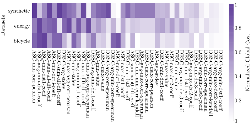
Figure 4: Learning performance of selected metrics for fixed bijections sorted according to the global cost obtained with all three datasets.

Overall, averaging metrics do not usually perform well or they are around the mean percentile. Discrete sine and cosine transformations may result in alternating positive and negative values that average to zero causing information loss. Instead, metrics that rely on minimal or maximal values convey more information. The ascending order maximizes or minimizes performance and vice versa for the descending order.

Figure 5 illustrates the optimality of fixed bijections under a varying number of children in the range $[2,14]$. Although structure does not show large influence on the synthetic and energy dataset, for the bicycle dataset with sparser plans [2] the agents’ positioning plays a more significant role. The following observations can be made for the bicycle dataset: (i) On average, the learning performance improves for all metrics by increasing the number of children per agent. (ii) The impact of the agents’ positioning is significantly higher for a binary tree as a higher deviation is observed among the metrics compared to trees with more than 8 children per agent.

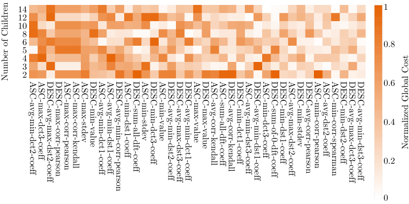
(a) Synthetic dataset

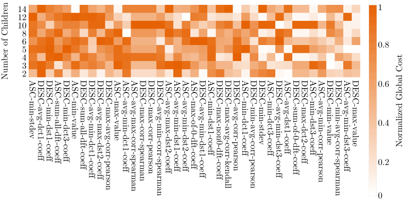
(b) Energy dataset

(c) Bicycle dataset

Figure 5: Learning performance of selected metrics for fixed bijections under varying number of children and sorted according to the global cost obtained with all three datasets.

IX-C Learning performance with dynamic bijections

Figure 6 compares the two online strategies for different datasets, baseline percentiles, memory offsets and thresholds. The optimality of the initial tree structure significantly influences learning performance. Starting from the $10^{th}$ percentile, self-adaptations are likely to decrease performance, nevertheless, to a low extent and there are cases in which performance improves as indicated by the area representing the standard deviation. In contrast, the $90^{th}$ percentile results in significantly lower global cost. The $50^{th}$ percentile shows a low performance improvement, mainly for the bicycle dataset. Note though that in case improved solutions are memorized or highly performing fixed bijections are applied, as shown in Section IX-B, learning performance can further improve.

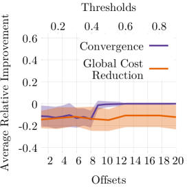
(a) Synthetic dataset, $10^{th}$ percentile

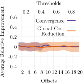
(b) Synthetic dataset, $50^{th}$ percentile

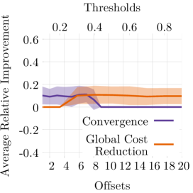
(c) Synthetic dataset, $90^{th}$ percentile

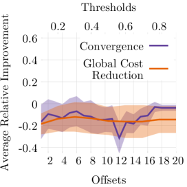
(d) Energy dataset, $10^{th}$ percentile

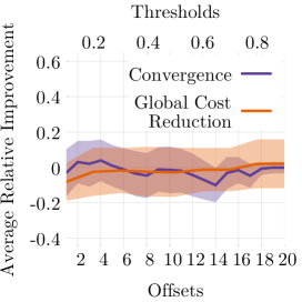
(e) Energy dataset, $50^{th}$ percentile

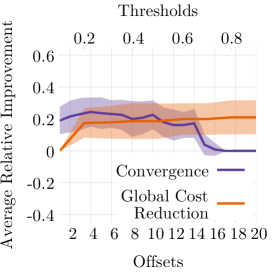
(f) Energy dataset, $90^{th}$ percentile

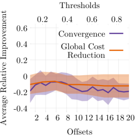
(g) Bicycle dataset, $10^{th}$ percentile

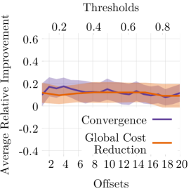
(h) Bicycle dataset, $50^{th}$ percentile

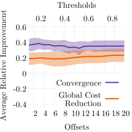
(i) Bicycle dataset, $90^{th}$ percentile

Figure 6: Learning performance of the two structural self-adaptation strategies for different datasets, baseline percentiles, memory offsets and thresholds.

The following observations can be made for the two strategies: (i) On average, the relative improvement of the convergence criterion with long-term memory is $-0.3\%$, $0.33\%$ and $11.01\%$ for the bicycle, energy and synthetic datasets respectively. For the global cost reduction criterion with short-term memory the respective numbers are $-1.7$%, $0.13\%$ and $7.03\%$. (ii) High memory offsets favor initialization with a highly performing tree structure ($10^{th}$ percentile), while low memory offsets favor initialization with a low performing tree ($90^{th}$ percentile). The likelihood of improving further a high-performing learning structure is lower unless solutions close to convergence are memorized. On the other hand, low-performing learning structures benefit from exploration with low memory offsets. (ii) The convergence criterion with long-term memory and low offsets maximize performance optimality across all baseline percentiles and datasets. (iii) Learning can be trapped into the first suboptimal solution for offsets higher than 10 using the convergence criterion with long-term memory as well as for threshold values lower than 0.2 using the global cost reduction with short-term memory,

Figure 7 illustrates the cumulative number of self-adaptations during the learning runtime for each of the two strategies and for different offsets, thresholds and datasets. Results are averaged out over all benchmark percentiles.

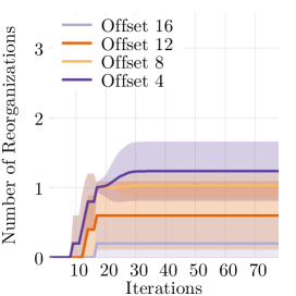
(a) Synthetic dataset, convergence criterion with long-term memory

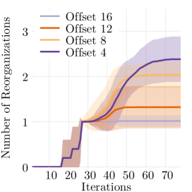
(b) Energy dataset, convergence criterion with long-term memory

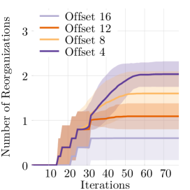
(c) Bicycle dataset, convergence criterion with long-term memory

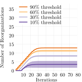
(d) Synthetic dataset, global cost reduction criterion with short-term memory

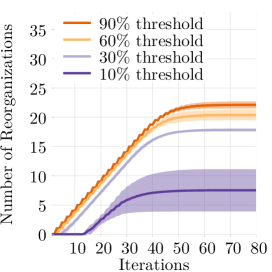
(e) Energy dataset, global cost reduction criterion with short-term memory

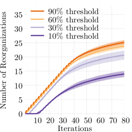
(f) Bicycle dataset, global cost reduction criterion with short-term memory

Figure 7: Cumulative number of self-adaptations over the learning runtime for the different strategies, memory offsets, thresholds and datasets.

The convergence criterion with long-term memory results in significantly lower structural self-adaptations. I-EPOS requires very few iterations, 10 or 15 for instance [2], to converge. Dividing the number of iterations with the offset iteration indicates the number of structural self-adaptation to expect. The higher the offset, the higher the optimality of the memorized solution and as a result the higher the likelihood of early termination at the next learning phase.

The global cost reduction criterion with short-term memory shows a higher number of self-adaptations, especially for the energy and bicycle dataset. The termination criterion measuring the slope of the global cost prevents early termination of I-EPOS by triggering self-adaptation early before convergence. This is especially the case for higher thresholds. Self-adaptations are triggered throughout the learning runtime for the bicycle dataset, while termination is observed around the $25^{th}$ and $40^{th}$ iteration for the synthetic and energy dataset.

X Conclusion and Future Work

This paper concludes that structure has a foundational role for the cost-effectiveness of decentralized pervasive intelligence as confirmed by the following: (i) Deterministic meta-feature criteria with which fixed structural self-adaptations are performed influence learning performance. (ii) Online structural self-adaptations can improve learning performance and prevent suboptimal trapped solutions, especially under low-performing initialization. A large-scale benchmark dataset for optimality evaluation is made openly available. It relies on real-world datasets of residential power demand, bike sharing and charging of electric vehicles. Millions of structural self-adaptation in networks of thousands of agents exchanging billion of learning messages provide representative performance profiles as shown with a comparison of parametric vs. non-parametric density estimations of the solutions space.

The construction of smarter online structural self-adaptations that consider the communication and computational cost of the agents’ repositioning is part of future work. Studying other communication structures besides trees can provide further insights and fundamental understanding.

References

- [1] F. Sadri, “Ambient intelligence: A survey,” ACM Computing Surveys (CSUR), vol. 43, no. 4, p. 36, 2011.
- [2] E. Pournaras, P. Pilgerstorfer, and T. Asikis, “Decentralized collective learning for self-managed sharing economies,” ACM Transactions on Autonomous and Adaptive Systems (TAAS), vol. 13, no. 2, p. 10, 2018.
- [3] S. Walczak and N. Cerpa, “Heuristic principles for the design of artificial neural networks,” Information and software technology, vol. 41, no. 2, pp. 107–117, 1999.
- [4] S. Karsoliya, “Approximating number of hidden layer neurons in multiple hidden layer bpnn architecture,” International Journal of Engineering Trends and Technology, vol. 3, no. 6, pp. 714–717, 2012.
- [5] E. Pournaras, “Optimality benchmark for combinatorial optimization,” Mar 2019. [Online]. Available: https://doi.org/10.6084/m9.figshare.7803005.v1
- [6] E. Pournaras, S. Jung, H. Zhang, X. Fang, and L. Sanders, “Socio-technical smart grid optimization via decentralized charge control of electric vehicles,” arXiv preprint arXiv:1701.06811, 2017.
- [7] R. T. Rockafellar, S. Uryasev et al., “Optimization of conditional value-at-risk,” Journal of risk, vol. 2, pp. 21–42, 2000.
- [8] Z. Allen-Zhu and E. Hazan, “Variance reduction for faster non-convex optimization,” in International Conference on Machine Learning, 2016, pp. 699–707.
- [9] M. Thapa, J. Espejo-Uribe, and E. Pournaras, “Measuring network reliability and repairability against cascading failures,” Journal of Intelligent Information Systems, pp. 1–22, 2017.
- [10] W. Yeoh, A. Felner, and S. Koenig, “Bnb-adopt: An asynchronous branch-and-bound dcop algorithm,” Journal of Artificial Intelligence Research, vol. 38, pp. 85–133, 2010.
- [11] A. Chechetka and K. Sycara, “No-commitment branch and bound search for distributed constraint optimization,” in Proceedings of the fifth international joint conference on Autonomous agents and multiagent systems. ACM, 2006, pp. 1427–1429.
- [12] A. Petcu and B. Faltings, “A scalable method for multiagent constraint optimization,” Tech. Rep., 2005.
- [13] D. Ye, M. Zhang, and A. V. Vasilakos, “A survey of self-organization mechanisms in multiagent systems,” IEEE Transactions on Systems, Man, and Cybernetics: Systems, vol. 47, no. 3, pp. 441–461, 2017.
- [14] A. Diaconescu, B. Porter, R. Rodrigues, and E. Pournaras, “Hierarchical self-awareness and authority for scalable self-integrating systems,” in 2018 IEEE 3rd International Workshops on Foundations and Applications of Self* Systems (FAS* W). IEEE, 2018, pp. 168–175.
- [15] E. Pournaras, “Epos software artifact,” Mar 2019. [Online]. Available: https://doi.org/10.1145/3277668
- [16] C. Hinrichs, S. Lehnhoff, and M. Sonnenschein, “Cohda: A combinatorial optimization heuristic for distributed agents,” in International Conference on Agents and Artificial Intelligence. Springer, 2013, pp. 23–39.
- [17] C. Hinrichs and M. Sonnenschein, “A distributed combinatorial optimisation heuristic for the scheduling of energy resources represented by self-interested agents.” IJBIC, vol. 10, no. 2, pp. 69–78, 2017.
- [18] W. Mason and D. J. Watts, “Collaborative learning in networks,” Proceedings of the National Academy of Sciences, vol. 109, no. 3, pp. 764–769, 2012.
- [19] C. Zhang and V. Lesser, “Coordinating multi-agent reinforcement learning with limited communication,” in Proceedings of the 2013 international conference on Autonomous agents and multi-agent systems. International Foundation for Autonomous Agents and Multiagent Systems, 2013, pp. 1101–1108.
- [20] C. Zhang, V. Lesser, and S. Abdallah, “Self-organization for coordinating decentralized reinforcement learning,” in Proceedings of the 9th International Conference on Autonomous Agents and Multiagent Systems: volume 1-Volume 1. International Foundation for Autonomous Agents and Multiagent Systems, 2010, pp. 739–746.
- [21] E. Pournaras, S. Yadhunathan, and A. Diaconescu, “Holarchic structures for decentralized deep learning: a performance analysis,” Cluster Computing, Feb 2019. [Online]. Available: https://doi.org/10.1007/s10586-019-02906-4
- [22] M. E. Celebi, “Improving the performance of k-means for color quantization,” Image and Vision Computing, vol. 29, no. 4, pp. 260–271, 2011.
- [23] P. S. Bradley and U. M. Fayyad, “Refining initial points for k-means clustering.” in ICML, vol. 98. Citeseer, 1998, pp. 91–99.
- [24] Y. Bengio, P. Simard, and P. Frasconi, “Learning long-term dependencies with gradient descent is difficult,” IEEE transactions on neural networks, vol. 5, no. 2, pp. 157–166, 1994.
- [25] R. Pascanu, T. Mikolov, and Y. Bengio, “On the difficulty of training recurrent neural networks,” in International Conference on Machine Learning, 2013, pp. 1310–1318.
- [26] J. Friedman, T. Hastie, and R. Tibshirani, The elements of statistical learning. Springer series in statistics New York, NY, USA:, 2001, vol. 1, no. 10.
- [27] S. Haykin, Neural networks: a comprehensive foundation. Prentice Hall PTR, 1994.
- [28] G. P. Gupta, M. Misra, and K. Garg, “An energy efficient distributed approach-based agent migration scheme for data aggregation in wireless sensor networks.” JIPS, vol. 11, no. 1, p. 148, 2015.
- [29] E. Pournaras, “Multi-level reconfigurable self-organization in overlay services,” Ph.D. dissertation, Delft University of Technology, 2013.
- [30] C. K. Yeo, B.-S. Lee, and M. H. Er, “A survey of application level multicast techniques,” Computer Communications, vol. 27, no. 15, pp. 1547–1568, 2004.
- [31] J. Risson and T. Moors, “Survey of research towards robust peer-to-peer networks: Search methods,” Computer networks, vol. 50, no. 17, pp. 3485–3521, 2006.
- [32] D. Mingxiao, M. Xiaofeng, Z. Zhe, W. Xiangwei, and C. Qijun, “A review on consensus algorithm of blockchain,” in 2017 IEEE International Conference on Systems, Man, and Cybernetics (SMC). IEEE, 2017, pp. 2567–2572.
- [33] E. Pournaras, “Agent-based planning portfolio,” Mar 2019. [Online]. Available: https://doi.org/10.6084/m9.figshare.7806548
- [34] E. Pournaras, M. Yao, and D. Helbing, “Self-regulating supply–demand systems,” Future Generation Computer Systems, vol. 76, pp. 73–91, 2017.
- [35] B. W. Silverman, Density estimation for statistics and data analysis. Routledge, 2018.