Communication for Generating Correlation:
A Unifying Survey

Abstract

The task of manipulating correlated random variables in a distributed setting has received attention in the fields of both Information Theory and Computer Science. Often shared correlations can be converted, using a little amount of communication, into perfectly shared uniform random variables. Such perfect shared randomness, in turn, enables the solutions of many tasks. Even the reverse conversion of perfectly shared uniform randomness into variables with a desired form of correlation turns out to be insightful and technically useful. In this article, we describe progress-to-date on such problems and lay out pertinent measures, achievability results, limits of performance, and point to new directions.

I Introduction

The ability to harness and work with randomness has been at the heart of information theory and modern computer science. Randomness has been used to model the “unknown” in information theory, be it a message produced by a source or the error introduced by a channel. In computer science, randomness is a resource that enables simpler, faster, and sometimes the only solution to many central problems. Of particular interest in this article is the use of randomness by a set of parties that are spread out geographically. Randomness enables such parties to generate secret keys and transmit messages securely [153]. It allows them to complete distributed computation tasks such as comparison of two strings using very few bits of communication [47, 186]. In Shannon theory, shared randomness is necessary to attain positive-rate channel codes for the arbitrary varying channel [31, 1]. Beyond these small sampling of applications which are directly related to the problems we shall consider in this article, there are many more applications of shared randomness, including synchronization, leader election, and consensus which are known to have no deterministic solutions for most multiparty settings of interest.

In many applications, it suffices to have a weak form of shared randomness instead of perfect uniform shared randomness. This leads to a quest for understanding weak forms of randomness and its limitations. A classic example of such a quest goes back to von Neumann (cf. [168]) who asked whether one could simulate an unbiased coin (uniform distribution over $\{0,1\}$) using a coin of unknown bias. His solution involves a sequence of tossing of pairs of coins till they show different outcomes. The first coin of this final pair is tantamount to a perfectly unbiased coin. If the biased coin has expected value $p$, then his solution tosses $1/(p(1-p))$ coins in expectation to get one unbiased coin. Improving the rate of usage of the biased coin and extending solutions to more general settings of imperfection, including correlations among coins, has lead to a rich theory of randomness extractors (cf. [152, 26, 101, 102, 90]).

In this paper, we shall be concerned with a different notion of imperfectness in randomness, namely that arising from distributed nature of problems. Many of the applications of randomness we listed earlier rely on, or can be interpreted as, a conversion of one form of such imperfect randomness into another, sometimes using communication between the parties. Focusing on two-party scenarios, we review research of this nature in this article and describe some of the unifying themes. We have divided these problems into four broad categories. We list these categories below, mention the sections where they appear, and highlight some interesting results in each category.

Generating common randomness using correlated observations and interactive communication (Section III)

The common randomness generation problem entails generating shared (almost) uniformly distributed bits at the parties, using initial correlated observations and interactive communication between the parties. When parties share copies of a uniform random string, they can accomplish several distributed tasks such as information-theoretically secure exchange of secrets. The study of common randomness generation is motivated by questions such as: what happens to such solutions when the parties share only some correlated variables? Is there an analog of the von Neumann solution that allows the parties to transform their random variables into identical ones with possibly less entropy? Does this require communication? If so, how much? Questions of this nature were raised in the seminal works of Maurer [126] and Ahlswede and Csiszár [2, 3] and continue to be the subject of active investigation.

A result of Gács and Körner [75] says that unless the parties shared bits to begin with, the number of bits of common randomness they can generate per observed independent sample without communicating goes to $0$. In fact, Witsenhausen [178] showed that the parties cannot even agree on a single bit without communicating. However, we shall see that by communicating the parties agree on more bits than they communicate [3]. These extra bits can be extracted as a secret key that is independent of the communication.

Generating secure common randomness, namely the problem of secret key agreement (Section IV)

The secret key agreement problem is closely related to common randomness generation and imposes an additional security requirement on the generated common randomness. Specifically, it requires that the generated common randomness be almost independent of the communication used to generate it. Such a common randomness will constitute a secret key that is information theoretically secure and can be used for cryptographic tasks such as secure message transmission and message authentication. The main result in this section says, roughly, that the rate of secret key that can be generated is given by the rate of common randomness minus the rate of communication. In fact, the two problems are intertwined and a complete characterization of communication-common randomness rate tradeoff will lead to a complete characterization of communication-secret key rate tradeoff.

Generating samples from a joint distribution without communicating (Section V)

In the next class of problems we consider, two parties observe correlated samples from a distribution and seek to generate samples from another. We consider the basic problems of approximation of output statistics, where the goal is to generate samples from a fixed distribution at the output of the channel by using a uniformly distributed input, and Wyner common information, where the goal is to generate samples from a fixed joint distribution using as few bits of shared randomness as possible. Another important problem in this class is that of correlated sampling where the knowledge of the joint distribution is not completely available to any single party.

From the many interesting results covered in this section, we highlight the following to pique the reader’s interest. A well-known result in probability theory and optimal transport theory states that given two distributions $\mathrm{P}$ and $\mathrm{Q}$, one can find a joint distribution $\mathrm{P}_{XY}$ such that $\mathrm{P}_{X}=\mathrm{P}$, $\mathrm{P}_{Y}=\mathrm{Q}$, and ${\mathrm{Pr}}\left(X\neq Y\right)=d\left(\mathrm{P},\mathrm{Q}\right)$, where $d\left(\cdot,\cdot\right)$ denotes variational distance. In fact, this is the least probability of disagreement possible for any such joint distribution $\mathrm{P}_{XY}$, which is known as the optimal coupling. We shall see that even when the knowledge of $\mathrm{P}$ and $\mathrm{Q}$ is only local, namely Party 1 knows $\mathrm{P}$ and Party 2 knows $\mathrm{Q}$, the same probability of disagreement as the optimal coupling can be attained up to a factor of $2$.

Generating samples from a distribution using communication (Section VI)

The final class of problems we consider is similar to the previous one, except that now the parties are allowed to communicate. Specific instances include the reverse Shannon theorem and interactive channel simulation, where the parties seek to simulate a given conditional distribution using as few bits of shared randomness and (noiseless) communication as possible; and simulation of interactive protocols, where the parties seek to simulate the distribution of transcripts of a given interactive protocol using minimum communication.

Many of these results have driven recent advances in communication complexity and even quantum information theory, and are also of independent interest. In particular, the reverse Shannon theorem says that, when the parties have access to shared randomness, they can simulate a channel by communicating at rate roughly equal to the mutual information between the input and the output, thereby establishing a “reverse” of Shannon’s classic channel capacity theorem. The interactive channel simulation problem is an abstraction that includes as a special case almost all problems we cover in this article. Thus, the reader might temper expectations for very general results for this problem. Note that the simulation problem is related closely to the (data) compression problem, which is well-studied in information theory. But there are some distinctions. While the latter necessitates obtaining an estimate for a given realization of a random variable, the former merely requires producing a copy of a random variable with a prescribed distribution. As a consequence, simulation of noisy channels typically requires less communication than compression; in simulation a part of communication can be realized from the shared randomness.

In addition to these topics, in Section II we review the basic tools from probability and randomness extraction that will be used throughout. Also, in Section VII we discuss some nonstandard applications of correlated sampling in approximate nearest neighbor search (locality sensitive hashing) and in showing hardness of approximation (the parallel repetition theorem). We conclude with pointers to extensions involving multiple parties and quantum correlation.

Many of the topics we cover are already the subjects of excellent review articles and monographs. See, for instance,  [164] for a review of information theoretic randomness extraction and its extension to the computational setting;  [60] for a chapter on information theoretic secret key agreement and wiretap channel;  [137] for common randomness and secret key generation by multiple parties; and the online manuscript [145] for simulation of protocols and its application to communication complexity. Our goal here is to present unifying themes underlying these diverse topics, with the hope of providing a treatment that is appealing to the information theorist as well as the computer scientist. To that end, we have reworked the presentation of some of the original proofs to bring out connections between various formulations.

Notation. All random variables are denoted by capital letters $X$, $Y$, etc., their realizations by $x$, $y$, etc., and their range sets by the corresponding calligraphic letters ${\mathcal{X}}$, ${\mathcal{Y}}$, etc.. The probability distribution of random variable $X$ is denoted by $\mathrm{P}_{X}$. The variational distance between $\mathrm{P}$ and $\mathrm{Q}$, denoted $d\left(\mathrm{P},\mathrm{Q}\right)$, is given by $\sup_{A\subseteq{\mathcal{X}}}\mathrm{P}(A)-\mathrm{Q}(A)$, which equals $1/2\sum_{x}|\mathrm{P}(x)-\mathrm{Q}(x)|$ for discrete distributions. The Kullback-Leibler (KL) divergence $D(\mathrm{P}\|\mathrm{Q})$ for discrete distributions $\mathrm{P}$ and $\mathrm{Q}$ equals $\sum_{x}\mathrm{P}(x)\log(\mathrm{P}(x)/\mathrm{Q}(x))$ when ${\tt supp}(\mathrm{P})\subseteq{\tt supp}(\mathrm{Q})$, and infinity otherwise. For random variables $X$ and $Y$, $I(X\wedge Y)=D(\mathrm{P}_{XY}\|\mathrm{P}_{X}\times\mathrm{P}_{Y})$ denotes the mutual information between $X$ and $Y$; we write $I(X\wedge(Y,Z))$ as $I(X\wedge Y,Z)$. The conditional mutual information $I(X\wedge Y|Z)$ denotes the conditional KL divergence $D(\mathrm{P}_{XY|Z}\|\mathrm{P}_{X|Z}\times\mathrm{P}_{Y|Z}|\mathrm{P}_{Z})={\mathbb{E}}_{Z}\left\{{D(\mathrm{P}_{XY|Z}\|\mathrm{P}_{X|Z}\times\mathrm{P}_{Y|Z})}\right\}$ and equals $I(X\wedge Y,Z)-I(X\wedge Z)$ (see [60] for further elaboration on our notation). Instead of instrumenting a consistent notation for the varied problems we consider, we abuse the notation $C$ and use it for expressing the fundamental limits in different contexts. The exact meaning will be clear from the context and the sub- and super-scripts used. Throughout, we shall denote asymptotic optimal quantities by $C$ and single-shot optimal quantities by $L$ .

II Preliminaries

In this section, we review some basic results and definitions that will be used throughout. Specifically, we review the leftover hash lemma, the maximal coupling lemma, and the basic measures of correlation such as maximal correlation and hypercontractivity. Further, we give a definition of interactive communication protocols with public coins and private coins, which will be used throughout. Finally, we provide a brief description of some informal terms that are common in information theory, but may not be familiar to a general reader. The presentation is brisk and introductory, and can be skipped if the reader is aware of these basic notions.

II-A Leftover hash and maximal coupling

We review two basic tools that underlie several proofs in this area. The leftover hash lemma allows us to extract uniform randomness that is a function of a given random variable $X$ and is almost independent of another random variable $Z$ correlated with $X$. Heuristically, the length of extractable uniform randomness is characterized by a measure of “leftover randomness” in $X$ given $Z$, such as the conditional entropy $H(X|Z)$. Even though this leftover randomness can be characterized using conditional entropy in the asymptotic setting, it turns out that a more relevant quantity in the non-asymptotic setting is the conditional min-entropy, to be defined below. The second result, termed the maximal coupling lemma, is classic in probability theory as well as analysis. Specifically, given two distributions $\mathrm{P}$ and $\mathrm{Q}$ on the same alphabet ${\mathcal{X}}$, the maximal coupling lemma yields a joint distribution $\mathrm{P}_{XY}$ with marginals $\mathrm{P}$ and $\mathrm{Q}$ such that ${\mathrm{Pr}}\left(X\neq Y\right)=d\left(\mathrm{P},\mathrm{Q}\right)$ (which is the least possible value of ${\mathrm{Pr}}\left(X\neq Y\right)$).

Traditionally, achievability proofs in information theory that use random binning arguments involved a randomly selected mapping from the set of all mappings with a given finite-size range. In fact, many of those proofs can be completed using a more economical construction that uses randomization over families of mappings with much smaller cardinality, termed a $2$-universal hash family, than the set of all mappings. This construction arose in the computer science literature in [47] and has gained popularity in information theory over the last decade. The leftover hash lemma uses $2$-universal hash families as well. We review their definition below.

Definition II.1 ($2$-Universal hash family).

A class of functions ${\mathcal{F}}$ from ${\mathcal{X}}$ to $\{0,1\}^{l}$ is called a $2$-universal hash family ($2$-UHF) if $\mathrm{P}\left(F(x)=F(x^{\prime})\right)\leq 2^{-l}$ for every $x\neq x^{\prime}\in{\mathcal{X}}$, where $F$ is distributed uniformly over the family ${\mathcal{F}}$.

Also, given random variables $(X,Z)$, we need a notion of residual randomness that will play a role in the leftover hash lemma and, at a high level, will constitute a single-shot variant of the conditional entropy $H(X|Z)$.

Definition II.2 (Min-entropy and conditional min-entropy).

The min-entropy of $\mathrm{P}$ is defined as

$$H_{\min}(\mathrm{P})\mathbin{:=}\min_{x\in{\cal X}}\log\frac{1}{\mathrm{P}(x)}.$$

For distributions $\mathrm{P}_{XZ}$ and $\mathrm{Q}_{Z}$, the conditional min-entropy of $\mathrm{P}_{XZ}$ given $\mathrm{Q}_{Z}$ is defined as

$$H_{\min}(\mathrm{P}_{XZ}|\mathrm{Q}_{Z})\mathbin{:=}\min_{x\in{\cal X},z\in\mathtt{supp}(\mathrm{Q}_{Z})}\log\frac{\mathrm{Q}_{Z}\left(z\right)}{\mathrm{P}_{XZ}\left(x,z\right)}.$$

Then, the conditional min-entropy of $\mathrm{P}_{XZ}$ given $Z$ is defined as

$$H_{\min}(\mathrm{P}_{XZ}|Z)\mathbin{:=}\max_{\mathrm{Q}_{Z}}H_{\min}(\mathrm{P}_{XZ}|\mathrm{Q}_{Z}),$$ (1)

where the maximization is taken over $\mathrm{Q}_{Z}$ satisfying $\mathtt{supp}(\mathrm{P}_{Z})\subseteq\mathtt{supp}(\mathrm{Q}_{Z})$.

While simple to define and operationally relevant (see [107]), the conditional min-entropy defined above is not easily amenable to theoretical analysis. It is more convenient to use its “smooth” variant defined next.

Definition II.3 (Smooth conditional min-entropy).

For distributions $\mathrm{P}_{XZ}$ and $\mathrm{Q}_{Z}$, and smoothing parameter $0\leq\varepsilon<1$, the smooth conditional min-entropy of $\mathrm{P}_{XZ}$ given $\mathrm{Q}_{Z}$ is defined as

$$H^{\varepsilon}_{\min}(\mathrm{P}_{XZ}|\mathrm{Q}_{Z})\mathbin{:=}\max_{\tilde{\mathrm{P}}_{XZ}\in{\cal B}_{\varepsilon}(\mathrm{P}_{XZ})}H_{\min}(\tilde{\mathrm{P}}_{XZ}|\mathrm{Q}_{Z}),$$ (2)

where

$${\cal B}_{\varepsilon}(\mathrm{P}_{XZ})\mathbin{:=}\big{\{}\tilde{\mathrm{P}}_{XZ}\in{\mathcal{P}}_{\tt sub}({\mathcal{X}}\times{\mathcal{Z}}):d(\tilde{\mathrm{P}}_{XZ},\mathrm{P}_{XZ})\leq\varepsilon\big{\}},$$

and ${\mathcal{P}}_{\tt sub}({\mathcal{X}}\times{\mathcal{Z}})$ is the set of subnormalized distributions on ${\mathcal{X}}\times{\mathcal{Z}}$, namely all nonnegative $\tilde{\mathrm{P}}_{XZ}$ such that $\sum_{x,z}\tilde{\mathrm{P}}_{XZ}(x,z)\leq 1$. The smooth conditional min-entropy of $\mathrm{P}_{XZ}$ given $Z$ is defined as

$$H^{\varepsilon}_{\min}(\mathrm{P}_{XZ}|Z)\mathbin{:=}\max_{\mathrm{Q}_{Z}}H^{\varepsilon}_{\min}(\mathrm{P}_{XZ}|\mathrm{Q}_{Z}),$$

where the maximization is taken over $\mathrm{Q}_{Z}$ satisfying $\mathtt{supp}(\mathrm{P}_{Z})\subseteq\mathtt{supp}(\mathrm{Q}_{Z})$.

Note that the maximum in (2) is taken over all subnormalized distributions, instead of just all distributions. This is simply for technical convenience; often, a smoothing over all distributions will suffice, but handling it requires more work.

An early variant of leftover hash lemma appeared in [26]. A version of the lemma closer to that stated below appeared in [101]; the appellation “leftover hash” was given in [102], perhaps motivated by the heuristic interpreation that the lemma provides a hash of “leftover randomness” in $X$ that is independent of side information. The form we present below, which is an extension of that in [90], is from [95] and can be proved using the treatment in [148]. This form involves additional side-information $V$ which takes values in a set ${\mathcal{V}}$ of finite cardinality $|{\mathcal{V}}|$.

Theorem II.1 (Leftover Hash Lemma).

Let $K=F(X)$ be a key of length $l$ generated by a mapping $F$ chosen uniformly at random from a $2$-UHF ${\mathcal{F}}$ and independently of $(X,Z,V)$. Then, it holds that

$$d\left(\mathrm{P}_{KZVF},\mathrm{P}_{{\mathcal{K}}}^{\mathtt{unif}}\times\mathrm{P}_{ZV}\times\mathrm{P}_{F}\right)$$

$$\leq 2\varepsilon+\frac{1}{2}\sqrt{2^{l-H^{\varepsilon}_{\min}(\mathrm{P}_{XZ}|Z)+\log|{\mathcal{V}}|}},$$

where $\mathrm{P}_{{\mathcal{K}}}^{\mathtt{unif}}$ is the uniform distribution on the range ${\mathcal{K}}$ of $F$.

Noting that $d\left(\mathrm{P}_{KZVF},\mathrm{P}_{{\mathcal{K}}}^{\mathtt{unif}}\times\mathrm{P}_{ZV}\times\mathrm{P}_{F}\right)$ equals ${\mathbb{E}}_{F}\left\{{d\left(\mathrm{P}_{F(X)ZV},\mathrm{P}_{{\mathcal{K}}}^{\mathtt{unif}}\times\mathrm{P}_{ZV}\right)}\right\}$, for a given source $\mathrm{P}_{XZV}$ we can derandomize the left-side and obtain a fixed mapping $f$ in ${\mathcal{F}}$ such that

$$d\left(\mathrm{P}_{f(X)ZV},\mathrm{P}_{{\mathcal{K}}}^{\mathtt{unif}}\times\mathrm{P}_{ZV}\right)\leq 2\varepsilon+\frac{1}{2}\sqrt{2^{l-H^{\varepsilon}_{\min}(\mathrm{P}_{XZ}|Z)+\log|{\mathcal{V}}|}}.$$

As a special case, we can find a fixed mapping $f$ for iid distribution $\mathrm{P}_{X^{n}Z^{n}}$ and $V$ given by a fixed mapping $g(X^{n},Z^{n})$. As a consequence, in our applications of leftover hash lemma below to common randomness generation and secret key agreement, we can attain the optimal rate using deterministic mappings.

In fact, we need not fix the distribution and the same derandomization can be extended to the case when the distribution $\mathrm{P}_{XZV}$ comes from a family ${\mathcal{P}}$ that is not too large. Interestingly, deterministic extractors even with one bit output do not exist for the broader class of sources with bounded min-entropy, i.e., ${\mathcal{P}}=\{\mathrm{P}_{X}:H_{\min}(\mathrm{P}_{X})\geq k\}$ for some threshold $k$, but one-bit deterministic extractors are possible for sources comprising two independent components each with min-entropy greater than a threshold [55]. A recent breakthrough result in this direction shows that we can find a deterministic extractor as long as the sum of min-entropies of two components is logarithmic in the input length (in bits) [54]. Review of this exciting topic is beyond the scope of this review article.

In a typical application, the random variable $Z$ represents the initial observation of an eavesdropper while the random variable $V$ represents an additional message revealed during the execution of a protocol. The result above roughly says that a secret key of length

$$l\simeq H^{\varepsilon}_{\min}(\mathrm{P}_{XZ}|Z)-\log|{\mathcal{V}}|$$

can be generated securely. The additional message $V$ could be included in the conditional side of the smooth min-entropy along with $Z$. But, the form above is more convenient since it does not depend on how $V$ is correlated to $(X,Z)$; an additional message of length $m$ decreases the key length by at most $m$ bit.

We remark that the smooth version is much easier to apply than the standard version with $\varepsilon=0$. Also, the proof of the smooth version is almost the same as that of the standard version and only applies triangle inequality in the first step additionally.

Next, we state the maximum coupling lemma, which in a more general form was shown by Strassen in [156] (see, also, [129, Lemma 11.3]).

Definition II.4.

Given two probability measures $\mathrm{P}$ and $\mathrm{Q}$ on the same alphabet ${\mathcal{X}}$, a coupling of $\mathrm{P}$ and $\mathrm{Q}$ is a pair of random variables $(X,Y)$ (or their joint distribution $\mathrm{P}_{XY}$) taking values in ${\mathcal{X}}\times{\mathcal{X}}$ such that the marginal of $X$ is $\mathrm{P}$ and of $Y$ is $\mathrm{Q}$. The set of all couplings of $\mathrm{P}$ and $\mathrm{Q}$ is denoted by ${\mathcal{P}}(\mathrm{P},\mathrm{Q})$.

Lemma II.2 (Maximal coupling lemma).

Given two probability measures $\mathrm{P}$ and $\mathrm{Q}$ on the same alphabet, for every $(X,Y)\in{\mathcal{P}}(\mathrm{P},\mathrm{Q})$,

$${\mathrm{Pr}}\left(X\neq Y\right)\geq d\left(\mathrm{P},\mathrm{Q}\right).$$

Furthermore, there exists a coupling which attains equality. (The equality-attaining coupling in the bound above is called a maximal coupling.)

II-B Maximal correlation and hypercontractivity

The notion of “correlation” lies at the heart of the topic of this paper. Various measures of correlation will be applied in presenting the results as well as in their proofs. One such measure is mutual information, which appears most prominently in our treatment. In this section, we review two other measures of correlation that are standard but perhaps are not known as widely.

The first measure captures roughly the maximum linear correlation that can be extracted from $X$ and $Y$. Specifically, given $\mathrm{P}_{XY}$, the maximal correlation $\rho_{m}(X,Y)$ between $X$ and $Y$ is defined as [151] (see, also,  [96, 77])

$$\rho_{m}(X,Y)=\max_{\begin{subarray}{c}f,g\,:\,{\mathbb{E}}\left[f(X)\right]={\mathbb{E}}\left[g(Y)\right]=0\\ \qquad\,{\mathbb{E}}\left[f^{2}(X)\right]={\mathbb{E}}\left[g^{2}(Y)\right]=1\end{subarray}}{\mathbb{E}}\left[f(X)g(Y)\right].$$

As an example, consider a binary symmetric source, denoted $BSS(\rho)$, $-1\leq\rho\leq 1$, comprising $(X_{1},X_{2})$ taking values in $\{0,1\}$ such that $\mathrm{P}_{X_{1}}\left(1\right)=1/2$ and

$$\mathrm{P}_{X_{1},X_{2}}\left(0,0\right)=\mathrm{P}_{X_{1},X_{2}}\left(1,1\right)=\frac{1}{4}(1+\rho).$$

For this source, the maximal correlation $\rho_{m}(X_{1},X_{2})=\rho$, and the functions $f$ and $g$ that achieve the maximum in the definition of $\rho_{m}$ are given by $f(x)=g(x)=(-1)^{x}$, $x\in\{0,1\}$. As another example, consider a Gaussian symmetric source, denoted $GSS(\rho)$, comprising jointly Gaussian $(X_{1},X_{2})$ with zero mean and covariance matrix given by

$$\begin{bmatrix}1&\rho\\ \rho&1\end{bmatrix}.$$

For this source the maximal correlation is attained by identity functions and is given by $\rho_{m}(X_{1},X_{2})=\rho$.

The second measure we describe, which is closely related to maximal correlation, is based on hypercontractivity (see [34, 83, 18, 5] for initial results and [138] for a historical review). Specifically, a distribution $\mathrm{P}_{XY}$ is $(p,q)$-hypercontractive for $1\leq q\leq p<\infty$ if for every bounded measurable function $f$ of $X$, the following holds:

$${\mathbb{E}}\left[|{\mathbb{E}}\left[f(X)|Y\right]|^{p}\right]^{\frac{1}{p}}\leq{\mathbb{E}}\left[|f(X)|^{q}\right]^{\frac{1}{q}}.$$ (3)

When $p=q$, (3) holds because of concavity of $p$-norm, which is sometimes known as contraction property of the conditional expectation operator. Since $p$-norm is monotonically non-decreasing in $p$, the $(p,q)$-hypercontractivity characterizes how much the contraction inequality can be strengthened. The condition above can be replaced equivalently by the following “Hölder” form: For all bounded measurable functions $f$ of $X$ and $g$ of $Y$

$${\mathbb{E}}\left[f(X)g(Y)\right]\leq\mathbb{E}\big{[}|f(X)|^{p^{\prime}}\big{]}^{\frac{1}{p^{\prime}}}\mathbb{E}\big{[}|g(Y)|^{q}\big{]}^{\frac{1}{q}},$$ (4)

where $p^{\prime}=p/(p-1)$ is the Hölder conjugate of $p\geq 1$. Again, when $p=q$, i.e., $p^{\prime}$ is the Hölder conjugate of $q$, (4) holds because of the Hölder inequality; the $(p,q)$-hypercontractivity also characterizes how much the Hölder inequality can be strengthened. The set of all $(p,q)$ satisfying the condition above is sometimes referred to as the hypercontractivity ribbon of $\mathrm{P}_{XY}$ and is denoted ${\mathcal{R}}(\mathrm{P}_{XY})$.

For $\mathrm{P}_{XY}$ given by a $BSS(\rho)$ or a $GSS(\rho)$, the following classic result of Bonami [34] (see, also, [18, 83]) characterizes the set of $p,q$ for which $\mathrm{P}_{XY}$ is $(p,q)$-hypercontractive.

Theorem II.3.

Suppose that $\mathrm{P}_{XY}$ corresponds to a $BSS(\rho)$ or a $GSS(\rho)$. Then, $\mathrm{P}_{XY}$ is $(p,q)$-hypercontractive if and only if

$$\frac{q-1}{p-1}\geq\rho^{2}.$$

Therefore, for $BSS(\rho)$ and $GSS(\rho)$ there is a close connection between hypercontractivity and maximal correlation $\rho_{m}(X,Y)$.

Ahlswede and Gács [5] highlighted a special parameter related to the hypercontractivity ribbon defined as

$$s^{*}(X,Y)=\lim_{p\rightarrow\infty}\inf_{q\,:\,(p,q)\in{\mathcal{R}}(\mathrm{P}_{XY})}\frac{q}{p}.$$

They showed in [5] that $s^{*}(X,Y)\geq\rho_{m}(X,Y)^{2}$. In fact, this inequality holds with equality for the cases of BSS and GSS (for further elaboration, see [8]).

The quantities $\rho_{m}(X,Y)$ and $s^{*}(X,Y)$ satisfy the following tensorization property: For independent $(X_{i},Y_{i})$, $1\leq i\leq n$,

$$\rho_{m}(X^{n},Y^{n}) =\max_{1\leq i\leq n}\rho_{m}(X_{i},Y_{i}),$$

$$s^{*}(X^{n},Y^{n}) =\max_{1\leq i\leq n}s^{*}(X_{i},Y_{i}).$$

Interestingly, the entire hypercontractivity ribbon tensorizes, $i.e.$,

$${\mathcal{R}}(X^{n},Y^{n})=\bigcap_{i=1}^{n}{\mathcal{R}}(X_{i},Y_{i}).$$ (5)

Note that information quantities such as mutual information satisfy an additivity (or subaddivity) property for independent $(X^{n},Y^{n})$, $i.e.$, $I(X^{n}\wedge Y^{n})=\sum_{i=1}^{n}I(X_{i}\wedge Y_{i})$. In fact, hypercontractivity has an information theoretic characterization (see [8], [136]), which also suggests a duality between additivity and tensorization (see [19]). An information theoretic characterization of the Brascamp-Lieb inequality, which includes the hypercontractivity bound as a special case, has been known earlier in the context of functional analysis [46]; for a recent treatment of the Brascamp-Lieb inequality in the context of information theory, see [20, 114].

II-C Communication protocols

The final concept we review in this section on preliminaries is that of interactive communication protocols, the key enabler of the tasks we consider in this paper. The reader may already have a heuristic notion of interactive communication in her mind, but a formal definition is necessary to specify the scope of our results, particularly of our converse bounds. Note that throughout we assume that the communication channel is noiseless which circumvents issues of synchronization that arise in interactive communication over noisy channels, and allows us to restrict ourselves to a simpler notion of interactive communication.

We restrict attention to tree protocols for interactive communication, which were introduced in the work of Yao [186]. Parties ${\mathcal{P}}_{1}$ and ${\mathcal{P}}_{2}$ observe input $X_{1}$ and $X_{2}$ generated from $\mathrm{P}_{X_{1}X_{2}}$, with ${\mathcal{P}}_{i}$ given access to $X_{i}$. Additionally, ${\mathcal{P}}_{i}$ has access to local randomness (private coins) $R_{{\tt pvt},i}$, $i\in\{1,2\}$, and both parties have access to shared randomness (public coins) $R_{{\tt pub}}$. We assume that random variables $R_{{\tt pvt},1},R_{{\tt pvt},2},R_{{\tt pub}}$ are mutually independent and are independent jointly of $(X_{1},X_{2})$. An interactive communication protocol $\pi$ is described by a labeled binary tree, where each node has a label from the set $\{1,2\}$. Starting from the root node, when the protocol reaches a node $v$ labeled $i$, ${\mathcal{P}}_{i}$ transmits a bit $b_{v}=b_{v}(X_{i},R_{{\tt pvt},i},R_{{\tt pub}})$, and the protocol proceeds to the left- or right-child of $v$ when $b_{v}$ is $1$ or $2$, respectively. The communication protocol terminates when a leaf node is reached, at which point each party declares an output. The (random) bit sequence representing the path from root to leaf is called the transcript of the protocol and is denoted by $\Pi$. Further, denoting by $O_{i}=O_{i}(X_{i},R_{{\tt pvt},i},R_{{\tt pub}},\Pi)$ the output of ${\mathcal{P}}_{i}$, $i\in\{1,2\}$, we say that the protocol $\pi$ has input $(X_{1},X_{2})$ and output $(O_{1},O_{2})$. The length of a protocol $\pi$, denoted $|\pi|$, is the maximum number of bits transmitted in any execution of the protocol and is given by the depth of the protocol tree for $\pi$. Figure 1 provides an illustration of a tree protocol. Note that the root is labeled $1$ denoting that ${\mathcal{P}}_{1}$ initiates the communication. Without loss of generality, this will be our assumption throughout the paper.

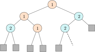
Figure 1: A two-party interactive protocol tree.

The protocols that allow a nonconstant shared randomness $R_{\tt pub}$ are referred to as public coin protocols. When shared randomness is not allowed, but local randomness is allowed, the protocols are referred to as private coin protocols. Finally, the protocols that do not allow private or shared randomness are called deterministic protocols.

The definition above allows the labels to switch arbitrarily along a path from the root to a leaf. A restricted class, termed $r$-round protocols, consists of protocols where the maximum number of times the label can switch along a path from the root to a leaf is $r$.

While the tree protocol structure described above is seemingly restrictive, typical lower bound proofs rely on some simple properties of such protocols.

1. Monotonicity of correlation. (cf. [126, 2]) For a private coin protocol $\pi$ with input $(X_{1},X_{2})$,

   $$I(X_{1}\wedge X_{2})\geq I(X_{1}\wedge X_{2}|\Pi).$$ (6)

   In particular, if $X_{1}$ and $X_{2}$ are independent, they remain so upon conditioning on $\Pi$.

2. Rectangle property. (cf. [186, 110]) For a private coin protocol $\pi$, denote by $p(\tau|x_{1},x_{2})$ the probability of $\Pi=\tau$ given that the input is $(x_{1},x_{2})$. Then, there exist functions $f_{\tau}$ and $g_{\tau}$ such that

   $$p(\tau|x_{1},x_{2})=f_{\tau}(x_{1})g_{\tau}(x_{2}),\quad\forall\,x_{1}\in{\mathcal{X}}_{1},x_{2}\in{\mathcal{X}}_{2}.$$

   For deterministic protocols, this implies that if a transcript $\tau$ appears for inputs $(x_{1},x_{2})$ and $(x_{1}^{\prime},x_{2}^{\prime})$, then it must appear for $(x_{1},x_{2}^{\prime})$ and $(x_{1}^{\prime},x_{2})$ as well. In other words, the set $\Pi^{-1}(\tau)$ constitutes a rectangle.

Both results above are, in essence, observations about the correlation we can build using tree protocols and are easy to prove. However, note that they are valid only for private coin protocols. When shared randomness (public coin) $R_{{\tt pub}}$ is used, the results above do not hold and the correlation has a more complicated structure. Nevertheless, even in this case, the results are recovered on conditioning additionally on $R_{{\tt pub}}$.

Closely related to the length of a protocol, namely the amount of information communicated in any execution of the protocol, is the so-called information cost of the protocol. Heuristically, information cost captures the number of bits of information that is revealed by the protocol. We recall two variants of information cost for private coin protocols.

The external information cost of a private coin protocol $\pi$ with inputs $(X_{1},X_{2})$ is given by [49]

$${\tt IC}_{\tt e}(\pi|X_{1},X_{2})=I(\Pi\wedge X_{1},X_{2}),$$

and its internal information cost is given by [16] (an early conference version appeared as [15])

$${\tt IC}_{\tt i}(\pi|X_{1},X_{2})=I(\Pi\wedge X_{1}|X_{2})+I(\Pi\wedge X_{2}|X_{1}).$$

Since

$${\tt IC}_{\tt e}(\pi|X_{1},X_{2})-{\tt IC}_{\tt i}(\pi|X_{1},X_{2})$$

$$=I(X_{1}\wedge X_{2})-I(X_{1}\wedge X_{2}|\Pi),$$ (7)

the following observation is equivalent to the monotonicity of correlation property (see, for instance, [62, 63, 16]):

$${\tt IC}_{\tt i}(\pi|X_{1},X_{2})\leq{\tt IC}_{\tt e}(\pi|X_{1},X_{2}).$$ (8)

The internal cost can be regarded as the amount of information conveyed between the parties, and the external cost can be regarded as the amount of information conveyed to an external observer of the transcripts. Thus, the inequality above says that parties share less information with each other than with an external observer, which is perhaps natural to expect since the inputs of the parties are correlated, and therefore, they have prior knowledge of each other’s input.

II-D Information theory parlance

In our narrative in this article, we shall be using the standard language of information theory. Some of the terms used are informal, but are standard occurrences in information theory parlance. Here we provide a quick listing of these terms for the benefit of the reader.

Several quantities in information theory are defined operationally as the optimal cost for a problem (such as minimum communication or maximum length of a secret key). These optimal costs are often characterized by a closed form formula which often finds applications beyond the original operational significance. The foremost example is that of channel capacity, which is an operationally defined quantity and is characterized as mutual information optimized over input distributions, but it has found use-cases beyond channel coding. Throughout this article, we endow information theoretic quantities with operational significance.

Another term that often shows up in Shannon theory is the so-called single-letter characterization, which we only describe informally here. Usually, operational quantities mentioned above can be easily characterized in terms of information theoretic quantities such as entropy, but involved random variables may take infinitely many values. Several open problems in information theory seek to express these quantities in terms of random variables taking finitely many values. Such expressions are called single-letter expressions in information theory. In the computer science literature, similar questions have been underlying the so-called direct-sum theorems where one seeks to solve a single instance of a problem using a protocol that solves multiple instances simultaneously.

Also, we take recourse to the notion of typical sets at several places. A formal definition of this notion can be found in the seminal textbook [60]. In particular, in the proof outline for Theorem III.2 we use the standard notion of $\mathrm{P}_{X}$-typical sets from [60], sometimes referred to as strongly typical sets, which is roughly the set of $n$-length sequences with normalized frequencies of each element $x$ close to $n\mathrm{P}_{X}\left(x\right)$.

III Common randomness generation

We begin with the common randomness (CR) generation problem. For simplicity, we restrict ourselves to private coin protocols in this section. As another simplifying assumption, we consider only the protocols that start at ${\mathcal{P}}_{1}$, namely the root of the protocol tree is labeled $1$. We also assume that the cardinalities $|{\mathcal{X}}_{1}|$ and $|{\mathcal{X}}_{2}|$ are finite; results for the Gaussian case are also highlighted whenever available.

Throughout this section, we restrict ourselves to source models where the parties are given correlated observations from a joint distribution. A richer model is a channel model where ${\mathcal{P}}_{1}$ can select an input $x\in{\mathcal{X}}$ for a channel $W:{\mathcal{X}}\to{\mathcal{Y}}$ whose output $Y$ is observed by ${\mathcal{P}}_{2}$. In addition, the parties can communicate over an error free channel using interactive protocols. We do not cover the results for this interesting setting; see [3, 165, 63] for initial results.

We present two variants of the CR generation problem: In the first, the amount of communication is fixed and the largest possible amount of CR that can be generated is characterized; and in the second, the amount of CR is fixed and the minimum amount of communication required is characterized. In principle, both variants above are closely related and studying one should shed light on the other. In practice, however, the specific formulations and the techniques considered in one case are difficult to transform to the other. Furthermore, the result we present in the second setting looks at very small probability of agreement, exponentially small in the CR length, and characterizes the minimum communication needed for generating a fixed length CR.

III-A CR using limited communication

The fundamental quantity of interest here is the following.

Definition III.1.

For jointly distributed random variables $(X_{1},X_{2})$, an integer $l$ is an $(\varepsilon,c,r)$-achievable CR length if there exists an $r$-round private coin protocol $\pi$ of length less than $c$ bits and with outputs $(S_{1},S_{2})$ such that, for a random string $S$ distributed uniformly over $\{0,1\}^{l}$,

$${\mathrm{Pr}}\left(S_{1}=S_{2}=S\right)\geq 1-\varepsilon.$$

The supremum over all $(\varepsilon,c,r)$-achievable CR lengths $l$ is denoted by $L_{\varepsilon,r}(c|X_{1},X_{2})$.

The random variable $S$ is referred to as an $(\varepsilon,c,r)$-CR of length $l$ using $\pi$; we omit the dependence on the parameters when it is clear from the context.

The formulation above was introduced by [2, 3] where they studied an asymptotic, capacity version of the quantity $L_{\varepsilon,r}(c|X_{1},X_{2})$.

Definition III.2 (Common randomness capacity).

For $R\geq 0$, $r\in{\mathbbm{N}}$, and an iid sequence $\{X_{1,i},X_{2,i}\}_{i=1}^{\infty}$, the $(\varepsilon,r)$-CR capacity for communication rate $R$, denoted $C_{\varepsilon,r}(R)$, is given by

$$C_{\varepsilon,r}(R)=\lim_{n\rightarrow\infty}\frac{1}{n}L_{\varepsilon,r}\big{(}nR|X_{1}^{n},X_{2}^{n}\big{)}.$$

Further, the $r$-round CR capacity for communication rate $R$, denoted $C_{r}(R)$, is given by $C_{r}(R)=\lim_{\varepsilon\rightarrow 0}C_{\varepsilon,r}(R)$. Finally, denote by $C(R)$ the supremum of $C_{r}(R)$ over $r\in{\mathbbm{N}}$.

The formulation of CR capacity in [3] allowed only two rounds of interaction, namely ${\mathcal{P}}_{1}$ upon observing $X_{1}^{n}$ sends $\Pi_{1}=f_{1}(X_{1}^{n})$ to ${\mathcal{P}}_{2}$, who in turn responds with $\Pi_{2}=f_{2}(\Pi_{1},X_{2}^{n})$. Furthermore, while [3] considered private coin $1$-round protocols, the extension to $2$ rounds was restricted to deterministic protocols. We denote this restricted notion of CR capacity using a $2$-round deterministic protocol of rate $R$ by $C_{2}^{d}(R)$; it is characterized as follows.

Theorem III.1 ([3]).

For $R\geq 0$ and random variable $(X_{1},X_{2})$ taking values in a finite set ${\mathcal{X}}_{1}\times{\mathcal{X}}_{2}$, we have

$$C_{2}^{d}(R)=\max_{\mathrm{P}_{UVX_{1}X_{2}}\in{\mathcal{P}}(R)}I(U\wedge X_{1})+I(V\wedge X_{2}|U)$$ (9)

where ${\mathcal{P}}(R)$ denotes the set of joint pmf $\mathrm{P}_{UVX_{1}X_{2}}$ such that the following conditions hold:

1. $\mathrm{P}_{UVX_{1}X_{2}}=\mathrm{P}_{X_{1}X_{2}}\mathrm{P}_{U|X_{1}}\mathrm{P}_{V|X_{2}U}$;

2. $U$ and $V$ take values in finite sets ${\mathcal{U}}$ and ${\mathcal{V}}$ such that $|{\mathcal{U}}|\leq|{\mathcal{X}}_{1}|+1$ and $|{\mathcal{V}}|\leq|{\mathcal{X}}_{2}||{\mathcal{U}}|+1$; and

3. $I(U\wedge X_{1}|X_{2})+I(V\wedge X_{2}|X_{1},U)\leq R$.

The expression on the right-side of (9) entails two interesting quantities: The first, $I(U\wedge X_{1})+I(V\wedge X_{2}|U)$ which in the view of the Markov relations $U-\!\!\!\!\circ\!\!\!\!-X_{1}-\!\!\!\!\circ\!\!\!\!-X_{2}$ and $V-\!\!\!\!\circ\!\!\!\!-(X_{2},U)-\!\!\!\!\circ\!\!\!\!-X_{1}$ equals $I(U,V\wedge X_{1},X_{2})$, and the second $I(U\wedge X_{1}|X_{2})+I(V\wedge X_{2}|X_{1},U)$ which appears in the constraints set and equals $I(U,V\wedge X_{1}|X_{2})+I(U,V\wedge X_{2}|X_{1})$. Both these quantities have a long history in the literature on network information theory; see, for instance, [181, 6, 183, 104]. In the computer science literature, these quantities have been rediscovered in a slightly different operational role, namely that of external and internal information costs defined in Section II. Specifically, consider a $2$-round protocol where ${\mathcal{P}}_{1}$ uses its private coin to sample $U$ using $\mathrm{P}_{U|X_{1}}$ and sends it to ${\mathcal{P}}_{2}$. Next, ${\mathcal{P}}_{2}$ samples $V$ using $\mathrm{P}_{V|X_{2},U}$ and sends it to ${\mathcal{P}}_{1}$. The overall joint distribution $\mathrm{P}_{UVX_{1}X_{2}}$ is maintained since $U-\!\!\!\!\circ\!\!\!\!-X_{1}-\!\!\!\!\circ\!\!\!\!-X_{2}$ and $V-\!\!\!\!\circ\!\!\!\!-(X_{2},U)-\!\!\!\!\circ\!\!\!\!-X_{1}$. Also, the protocol is a tree protocol since $|{\mathcal{U}}|$ and $|{\mathcal{V}}|$ can be restricted to be finite. It is easy to see that any $2$-round private coin protocol can be expressed similarly in terms of $U$ and $V$. Thus, (9) can be restated as follows:

$$C_{2}^{d}(R)=\max_{\pi:{\tt IC}_{\tt i}(\pi|{X_{1},X_{2}})\leq R}{\tt IC}_{\tt e}(\pi|X_{1},X_{2}),$$ (10)

where the maximum is restricted to $2$-round private coin protocols $\pi$. Note that while the “$n$-fold” problem for $C_{2}^{d}(R)$ did not allow randomization, the “single-letter” characterization above entails optimization over private coin protocols.

The result can be extended to the case when arbitrary (but fixed) round private coin protocols are allowed. This extension and its proof are perhaps known to specialists in this area, but it has not been formally reported anywhere. However, glimpses of this result can be seen, for instance, in [189], [80], [157], [117], and [78].

In fact, it is interesting to track the history of this result in information theory and computer science. Following the work of Ahlswede and Csiszár [2, 3], a multiparty extension of the CR agreement problem appeared in a specialized model appeared in [61] and for the related problem of secret key agreement in [62]. A result very similar to Theorem III.2 seems to have appeared first in [189, Theorem 5.3], albeit without a complete proof. The schemes in all these works in the information theory literature are based on the classic binning technique of Wyner and Ziv [183], which was also used for function computation in [141]. This is where the intersection with the computer science literature first appears. Specifically, the rates achieved by Wyner-Ziv binning entail terms of the form $I(U\wedge X|Y)$, namely internal information complexity of one round protocols. This quantity was used as a measure of information complexity for function computation in [15, 38], following the pioneering works [49, 13]. Interestingly, the same result as [38] was obtained independently in [121, 122] in the information theory literature, where the information complexity quantities facilitated Wyner-Ziv binning in the scheme; the converse proof in [122] used a method introduced in [104], which was slightly different from the “embedding” used in [38]. Till this point, these two lines of works bringing in information complexity emerged independently. This seems to have changed after a workshop at Banff on Interactive Information Theory in 2012 where the authors of [38] and [122] participated and learnt of these two views on the same results. Subsequently, review articles such as [36] appeared, but still the application of information complexity to CR generation was not explicitly mentioned anywhere. This connection was exploited in works such as [163] (for instance, [163, Eqn. 14] is a single-shot counterpart of (7)), but the first instance where this connection was explicitly mentioned is [78].

Let $C^{d}(R)$ be the analog of $C(R)$ for deterministic communication protocols. Our characterization of $C^{d}(R)$ and $C(R)$ involves a function $f(R)$, which is an extension of the function on the right-side of (10) to multiple rounds, given by

$$f(R):=\sup_{\pi:{\tt IC}_{\tt i}(\pi|{X_{1},X_{2}})\leq R}{\tt IC}_{\tt e}(\pi|{X_{1},X_{2}}),$$ (11)

where the supremum is taken over all protocols with arbitrary (finite) number of rounds.

Theorem III.2.

For $R\geq 0$ and random variable $(X_{1},X_{2})$ taking values in a finite set ${\mathcal{X}}_{1}\times{\mathcal{X}}_{2}$, we have

$$C^{d}(R)=f(R)$$ (12)

and

$$C(R)=\sup_{t\geq 0}f(R-t)+t.$$ (13)

Proof of Theorem III.2 for deterministic protocols

We first prove the lower bound (converse) part of (12), i.e., $C^{d}(R)\geq f(R)$. Consider an $(\varepsilon,c,r)$-CR $S$ of length $l$ that can be recovered using an $r$-round deterministic communication protocol $\pi_{n}$ with input $(X_{1}^{n},X_{2}^{n})$ where $X_{i}^{n}=(X_{i1},...,X_{in})$ denotes the observation of ${\mathcal{P}}_{i}$, $i=1,2$. For simplicity, we assume that ${\mathcal{P}}_{1}$ is the last party to communicate; the other case can be handled similarly. Denote by $\Pi_{i}$ the communication sent in round $i$ and by $S_{1}$ the estimate of $S$ formed at ${\mathcal{P}}_{1}$. Since $S$ is uniformly distributed, by Fano’s inequality we have

$$l\leq H(S_{1})+\varepsilon l+1.$$ (14)

Thus, it suffices to bound $H(S_{1})$. We show that there exists an $r$-round private coin protocol $\pi_{1}$ with input $(X_{1},X_{2})$ such that $H(S_{1})\leq n{\tt IC}_{\tt e}(\pi_{1}|X_{1},X_{2})$ and $n{\tt IC}_{\tt i}(\pi_{1}|X_{1},X_{2})\lesssim c$. Specifically, abbreviating $X_{ij}^{k}=X_{ij},...,X_{ik}$, $i=1,2$ and with $J$ distributed uniformly over $\{1,...,n\}$ independently of $(\Pi,X_{1}^{n},X_{2}^{n})$, let $U_{1}=(X_{11},...,X_{1(J-1)},X_{2(J+1)},...,X_{2n},\Pi_{1},J)$, $U_{i}=\Pi_{i}$ for $1<i<r$, and $U_{r}=(\Pi_{r},S_{1})$. The following Markov relation can be shown to hold: For $0\leq i\leq r$

$$U_{1}-\!\!\!\!\circ\!\!\!\!-X_{1J}-\!\!\!\!\circ\!\!\!\!-X_{2J},$$

$$U_{i+1}-\!\!\!\!\circ\!\!\!\!-(U^{i},X_{1J})-\!\!\!\!\circ\!\!\!\!-X_{2J},\quad i\text{ even},i\geq 2,$$

$$U_{i+1}-\!\!\!\!\circ\!\!\!\!-(U^{i},X_{2J})-\!\!\!\!\circ\!\!\!\!-X_{1J},\quad i\text{ odd},i\geq 1.$$ (15)

The Markov relations can be obtained as a consequence of monotonicity of correlation property of interactive communication (see Section II-C). We outline the proof for $U_{i+1}-\!\!\!\!\circ\!\!\!\!-(U^{i},X_{1J})-\!\!\!\!\circ\!\!\!\!-X_{2J}$ for even $i<r$; the remaining can be derived similarly. Consider a hypothetical situation in which ${\mathcal{P}}_{1}$ observes $(X_{1(j+1)}^{n},X_{2(j+1)}^{n})$ and ${\mathcal{P}}_{2}$ observes $(X_{11}^{j},X_{21}^{j})$, which are independent. First, ${\mathcal{P}}_{1}$ and ${\mathcal{P}}_{2}$ exchange $X_{2(j+1)}^{n}$ and $X_{11}^{j}$ so that ${\mathcal{P}}_{1}$ obtains $X_{1}^{n}$ and ${\mathcal{P}}_{2}$ obtains $X_{2}^{n}$, which enables them to simulate the transcript $\Pi^{i}$ via interactive communication. Then, using the monotonicity of correlation property, we get

$$0 =I(X_{1(j+1)}^{n},X_{2(j+1)}^{n}\wedge X_{11}^{j},X_{21}^{j})$$

$$\geq I(X_{1(j+1)}^{n},X_{2(j+1)}^{n}\wedge X_{11}^{j},X_{21}^{j}|X_{11}^{j},X_{2(j+1)}^{n},\Pi^{i})$$

$$=I(X_{1(j+1)}^{n},X_{2(j+1)}^{n},\Pi_{i+1}\wedge X_{11}^{j},X_{21}^{j}|X_{11}^{j},X_{2(j+1)}^{n},\Pi^{i})$$

$$\geq I(\Pi_{i+1}\wedge X_{2j}|X_{1j},X_{11}^{j-1},X_{2(j+1)}^{n},\Pi^{i})$$

where the second identity uses the fact that $\Pi_{i+1}$ is a function of $X_{1}^{n}$ given $\Pi^{i}$. Thus, $I(\Pi_{i+1}\wedge X_{2J}|U^{i})=0$, which given (15).

By noting the Markov relation $\Pi_{i}-\!\!\!\!\circ\!\!\!\!-(X_{1}^{n},\Pi^{i-1})-\!\!\!\!\circ\!\!\!\!-X_{2}^{n}$ for odd $i$ and $\Pi_{i}-\!\!\!\!\circ\!\!\!\!-(X_{2}^{n},\Pi^{i-1})-\!\!\!\!\circ\!\!\!\!-X_{1}^{n}$ for even $i$, we can get

$$H(S_{1})$$

$$\leq I(S_{1},\Pi\wedge X_{1}^{n},X_{2}^{n})$$

$$=\sum_{i=1:\mathrm{odd}}^{r-2}I(\Pi_{i}\wedge X_{1}^{n}|\Pi^{i-1})$$

$$~{}~{}~{}+\sum_{i=2:\mathrm{even}}^{r-1}I(\Pi_{i}\wedge X_{2}^{n}|\Pi^{i-1})+I(S_{1},\Pi_{r}\wedge X_{1}^{n}|\Pi^{r-1})$$

$$=H(X_{1}^{n})+\sum_{i=1:\mathrm{odd}}^{r-2}\big{[}H(X_{2}^{n}|\Pi^{i})-H(X_{1}^{n}|\Pi^{i})\big{]}$$

$$~{}~{}~{}+\sum_{i=2:\mathrm{even}}^{r-1}\big{[}H(X_{1}^{n}|\Pi^{i})-H(X_{2}^{n}|\Pi^{i})\big{]}-H(X_{1}^{n}|S_{1},\Pi^{r})$$

$$\leq nH(X_{1J})+\sum_{i=1:\mathrm{odd}}^{r-2}\big{[}H(X_{2}^{n}|\Pi^{i})-H(X_{1}^{n}|\Pi^{i})\big{]}$$

$$~{}~{}~{}+\sum_{i=2:\mathrm{even}}^{r-1}\big{[}H(X_{1}^{n}|\Pi^{i})-H(X_{2}^{n}|\Pi^{i})\big{]}-nH(X_{1,J}|U^{r})$$

$$=n\bigg{[}H(X_{1J})+\sum_{i=1:\mathrm{odd}}^{r-2}\big{[}H(X_{2J}|U^{i})-H(X_{1J}|U^{i})\big{]}$$

$$~{}~{}~{}+\sum_{i=2:\mathrm{even}}^{r-1}\big{[}H(X_{1J}|U^{i})-H(X_{2J}|U^{i})\big{]}-H(X_{1J}|U^{r})\bigg{]}$$

$$=nI(U^{r}\wedge X_{1J},X_{2J}),$$

where the second last equality uses

$$H(X_{1}^{n}|\Pi^{i})-H(X_{2}^{n}|\Pi^{i})$$

$$=n\big{[}H\big{(}X_{1J}|X_{11}^{J-1},X_{2(J+1)}^{n},\Pi^{i},J\big{)}$$

$$~{}~{}~{}-H\big{(}X_{2J}|X_{11}^{J-1},X_{2(J+1)}^{n},\Pi^{i},J\big{)}\big{]}.$$ (16)

Also, for deterministic protocols, the monotonicity of correlation property is the same as

$$H(\Pi)\geq H(\Pi\mid X_{1}^{n})+H(\Pi\mid X_{2}^{n}),$$

which together with the Fano inequality gives

$$H(\Pi) \geq I(\Pi\wedge X_{1}^{n}|X_{2}^{n})+I(\Pi\wedge X_{2}^{n}|X_{1}^{n})$$

$$\geq I(S_{1},\Pi\wedge X_{1}^{n}|X_{2}^{n})+I(S_{1},\Pi\wedge X_{2}^{n}|X_{1}^{n})-l\varepsilon-1.$$

In order to derive the single-letter characterization, again by noting the Markov relation $\Pi_{i}-\!\!\!\!\circ\!\!\!\!-(X_{1}^{n},\Pi^{i-1})-\!\!\!\!\circ\!\!\!\!-X_{2}^{n}$ for odd $i$ and $\Pi_{i}-\!\!\!\!\circ\!\!\!\!-(X_{2}^{n},\Pi^{i-1})-\!\!\!\!\circ\!\!\!\!-X_{1}^{n}$ for even $i$, we can get

$$I(S_{1},\Pi\wedge X_{1}^{n}|X_{2}^{n})+I(S_{1},\Pi\wedge X_{2}^{n}|X_{1}^{n})$$

$$=\sum_{i=1:\mathrm{odd}}^{r-2}I(\Pi_{i}\wedge X_{1}^{n}|X_{2}^{n},\Pi^{i-1})$$

$$~{}~{}~{}+\sum_{i=2:\mathrm{even}}^{r-1}I(\Pi_{i}\wedge X_{1}^{n}|X_{2}^{n},\Pi^{i-1})$$

$$~{}~{}~{}+I(S_{1},\Pi_{r}\wedge X_{1}^{n}|X_{2}^{n},\Pi^{r-1})$$

$$=H(X_{1}^{n}|X_{2}^{n})+\sum_{i=1:\mathrm{odd}}^{r-2}\big{[}H(X_{2}^{n}|X_{1}^{n},\Pi^{i})-H(X_{1}^{n}|X_{2}^{n},\Pi^{i})\big{]}$$

$$~{}~{}~{}+\sum_{i=2:\mathrm{even}}^{r-1}\big{[}H(X_{1}^{n}|X_{2}^{n},\Pi^{i})-H(X_{2}^{n}|X_{1}^{n},\Pi^{i})\big{]}$$

$$~{}~{}~{}-H(X_{1}^{n}|X_{2}^{n},S_{1},\Pi^{r})$$

$$\geq nH(X_{1J}|X_{2,J})$$

$$~{}~{}~{}+\sum_{i=1:\mathrm{odd}}^{r-2}\big{[}H(X_{2}^{n}|X_{1}^{n},\Pi^{i})-H(X_{1}^{n}|X_{2}^{n},\Pi^{i})\big{]}$$

$$~{}~{}~{}+\sum_{i=2:\mathrm{even}}^{r-1}\big{[}H(X_{1}^{n}|X_{2}^{n},\Pi^{i})-H(X_{2}^{n}|X_{1}^{n},\Pi^{i})\big{]}$$

$$~{}~{}~{}-nH(X_{1,J}|X_{2,J},U^{r})$$

$$=n\bigg{[}H(X_{1J}|X_{2,J})$$

$$~{}~{}~{}+\sum_{i=1:\mathrm{odd}}^{r-2}\big{[}H(X_{2J}|X_{1J},U^{i})-H(X_{1J}|X_{2J},U^{i})\big{]}$$

$$~{}~{}~{}+\sum_{i=2:\mathrm{even}}^{r-1}\big{[}H(X_{1J}|X_{2J},U^{i})-H(X_{2J}|X_{1J},U^{i})\big{]}$$

$$~{}~{}~{}-nH(X_{1J}|X_{2J},U^{r})\bigg{]}$$

$$=n\big{[}I(U^{r}\wedge X_{1J}|X_{2J})+I(U^{r}\wedge X_{2J}|X_{1J})\big{]},$$

where the second last inequality again uses (16) along with the identity

$$H(X_{2}^{n}|X_{1}^{n},\Pi^{i})-H(X_{1}^{n}|X_{2}^{n},\Pi^{i})$$

$$=H(X_{1}^{n}|\Pi^{i})-H(X_{2}^{n}|\Pi^{i}).$$

Therefore, noting that $(X_{1J},X_{2J})$ has the same distribution as $(X_{1},X_{2})$, in the limits as $n$ goes to infinity and $\varepsilon$ goes to zero (in that order), we get by (14) and the bounds above that the rate of CR is bounded above by $f(R)$ defined in (11). Also, to claim that $U^{r}$ correspond to a protocol, we need to bound the cardinalities of their support sets. Under our assumption of finite $|{\mathcal{X}}_{1}|$ and $|{\mathcal{X}}_{2}|$, we can restrict the cardinalities of ${\mathcal{U}}_{i}$ to be finite using the support lemma [60, Lemma 15.4].

For the proof of the upper bound (achievability) of the deterministic case, we begin with an outline of the proof for achieving $f(R)$ restricted to $r=1$, namely achieving

$$\max_{\begin{subarray}{c}U:U-\!\!\!\!\circ\!\!\!\!-X_{1}-\!\!\!\!\circ\!\!\!\!-X_{2}\\ \qquad I(U\wedge X_{1}|X_{2})\leq R\end{subarray}}I(U\wedge X_{1}).$$ (17)

We use standard typical set arguments to complete the proof [57, 59, 60]. Consider a random codebook

$${\mathcal{C}}=\{U^{n}(i,j),1\leq i\leq\lceil 2^{nR}\rceil,1\leq j\leq\lceil 2^{n\gamma}\rceil\},$$

where $U^{n}(i,j)\in{\mathcal{U}}^{n}$ are iid (for different $i,j$) and uniformly distributed over the $\mathrm{P}_{U}$-typical set. Consider the following protocol:

1. ${\mathcal{P}}_{1}$ finds the smallest $i$ for which there exists a $j$ such that $(X_{1}^{n},U^{n}(i,j))$ is $\mathrm{P}_{UX_{1}}$-typical. Let $\Pi_{1}$ denote this smallest index $i$ and $Y_{1}$ denote the sequence $U^{n}(i,j)$ identified above.

2. ${\mathcal{P}}_{1}$ sends $\Pi_{1}$ to ${\mathcal{P}}_{2}$.

3. ${\mathcal{P}}_{2}$ searches for the smallest index $j$ such that $(X_{2}^{n},U^{n}(\Pi_{1},j))$ is $\mathrm{P}_{UX_{2}}$-typical. Denote by $Y_{2}$ the sequence $U^{n}(\Pi_{1},j)$.

The standard covering and packing arguments in multiterminal information theory (cf. [60]) imply that for $\gamma=I(U\wedge X_{2})-2\delta$ and $R=I(U\wedge X_{1}|X_{2})+3\delta$, the protocol above yields $Y_{1}$ and $Y_{2}$ that agree with large probability (over the random input and the random codebook). Furthermore, for every fixed realization of the codebook ${\mathcal{C}}$, it can be shown using standard typical set arguments that with ${\mathcal{T}}$ denoting the $\mathrm{P}_{UX_{1}}$-typical set

$${\mathrm{Pr}}\left(Y_{1}=u^{n}(i,j)\right) \leq\mathrm{P}_{X_{1}^{n}}\left(\{x^{n}:(u^{n},x^{n})\in{\mathcal{T}}\}\right)$$

$$\leq\exp\left(-nI(U\wedge X_{1})+o(n)\right).$$

Therefore, using the leftover hash lemma (see Theorem II.1) with $Y_{1}$ in the role of $X$ and $(Z,V)$ set to constants, and noting that the min-entropy of $Y_{1}$ is roughly $nI(U\wedge X_{1})$ by the previous bound, there exists a fixed function $g$ of $Y_{1}$ and $S$ consisting of roughly $nI(U\wedge X_{1})$ uniformly distributed random bits such that $S_{1}=g(Y_{1})$ satisfies $d\left(\mathrm{P}_{S_{1}},\mathrm{P}_{S}\right)\leq\varepsilon/2$. Using the maximal coupling lemma (see Lemma II.2), there exists a joint distribution $\mathrm{P}_{S_{1}S}$ with the same marginals as the original $S_{1}$ and $S$ such that ${\mathrm{Pr}}\left(S_{1}\neq S\right)\leq\varepsilon/2$. Therefore, for $\mathrm{P}_{X_{1}^{n}X_{2}^{n}S_{1}S}=\mathrm{P}_{X_{1}^{n}X_{2}^{n}S_{1}}\mathrm{P}_{S|S_{1}}$, we have

$${\mathrm{Pr}}\left(S=S_{1}=S_{2}\right) \geq{\mathrm{Pr}}\left(S=S_{1}\right)+{\mathrm{Pr}}\left(S_{1}=S_{2}\right)-1$$

$$\geq 1-\varepsilon,$$

for all $n$ sufficiently large. The final step in our protocol is now simple:

1. ${\mathcal{P}}_{i}$ outputs $S_{i}=g(Y_{i})$, $i=1,2$.

Note that the rate of communication is no less than $R=I(U\wedge X_{1}|X_{2})+3\delta$ and the rate of CR generated is $I(U\wedge X_{1})$. Furthermore, since the mapping $g$ can be found for any fixed realization of the codebook ${\mathcal{C}}$, we can derandomize the argument above to obtain a deterministic scheme. This completes the achievability proof for the rate in (17). To extend the proof to $r=2$, we repeat the construction above but conditioned on the previously generated CR, namely the sequence $U^{n}$ found in Step 1. The analysis will remain the same in essence, except that the mutual information quantities will be replaced by conditional mutual information given $U$; leftover hash will be applied to the overall shared sequence pair. Extension to further higher number of rounds is obtained by repeating this argument recursively. ∎

Extending the proof to private coin protocols

We now move to the general case where private coin protocols are allowed and prove (13). Achievability follows from the time sharing between a (deterministic) scheme attaining CR rate $f(R-t)$ with communication rate $R-t$ and a trivial private coin scheme attaining CR rate $t$ with communication rate $t$ which simply shares $t$ random bits over the communication channel. To extend the proof of converse to private coin protocols, we assume without loss of generality that private randomness of ${\mathcal{P}}_{1}$ and ${\mathcal{P}}_{2}$, respectively, are given by iid sequences $W_{1}^{n}$ and $W_{2}^{n}$. We can then use the proof for the deterministic case to get a single-shot protocol $\pi_{1}$ such that the rate of CR is less than ${\tt IC}_{\tt e}(\pi_{1}|(X_{1},W_{1}),(X_{2},W_{2}))$ and the rate of communication is more than ${\tt IC}_{\tt i}(\pi_{1}|(X_{1},W_{1}),(X_{2},W_{2}))$. To complete the proof, we show that there exists another private coin protocol $\pi_{1}^{\prime}$ and nonnegative $t$ such that

$${\tt IC}_{\tt e}(\pi_{1}|(X_{1},W_{1}),(X_{2},W_{2}))={\tt IC}_{\tt e}(\pi_{1}^{\prime}|X_{1},X_{2})+t,$$ (18)

and

$${\tt IC}_{\tt i}(\pi_{1}|(X_{1},W_{1}),(X_{2},W_{2}))={\tt IC}_{\tt i}(\pi_{1}^{\prime}|X_{1},X_{2})+t,$$ (19)

whereby it follows that $C(R)\leq f(R-t)+t$ for some $t\geq 0$.

To see (18) and (19), for transcript $U^{r}$ of protocol $\pi_{1}$ and for every $1\leq i\leq r$, by the monotonicity of correlation we get

$$I(W_{1}\wedge X_{2},W_{2}|X_{1},U^{i}) =0,$$

$$I(W_{2}\wedge X_{1},W_{1}|X_{2},U^{i}) =0.$$

Indeed, the first relation follows by noting that $(X_{1},U^{i})$ is an interactive communication protocol for two parties where ${\mathcal{P}}_{1}$ observes $W_{1}$ and ${\mathcal{P}}_{2}$ observes $(X_{1},X_{2},W_{2})$; the second one can be obtained similarly. Using these conditional independence relations, for odd $i$ we have

$$I(U_{i}\wedge X_{2}|X_{1},U^{i-1})$$

$$\leq I(U_{i},W_{1}\wedge X_{2},W_{2}|X_{1},U^{i-1})$$

$$=I(W_{1}\wedge X_{2},W_{2}|X_{1},U^{i-1})$$

$$~{}~{}~{}+I(U_{i}\wedge X_{2},W_{2}|X_{1},W_{1},U^{i-1})$$

$$=0.$$

Similarly, for even $i$, we have

$$I(U_{i}\wedge X_{1}|X_{2},U^{i-1})=0.$$

Thus, we find that $U^{r}$ constitutes transcript of an interactive protocol $\pi_{1}^{\prime}$ with observation $(X_{1},X_{2})$. Furthermore, we can expand the information costs of $\pi_{1}$ as follows:

$${\tt IC}_{\tt e}(\pi_{1}|(X_{1},W_{1}),(X_{2},W_{2}))$$

$$=I(U^{r}\wedge X_{1},W_{1},X_{2},W_{2})$$

$$=\sum_{i:\mathrm{odd}}I(U_{i}\wedge X_{1},W_{1}|U^{i-1})+\sum_{i:\mathrm{even}}I(U_{i}\wedge X_{2},W_{2}|U^{i-1})$$

$$=\sum_{i:\mathrm{odd}}\big{[}I(U_{i}\wedge X_{1}|U^{i-1})+I(U_{i}\wedge W_{1}|X_{1},U^{i-1})\big{]}$$

$$~{}~{}~{}+\sum_{i:\mathrm{even}}\big{[}I(U_{i}\wedge X_{2}|U^{i-1})+I(U_{i}\wedge W_{2}|X_{2},U^{i-1})\big{]}$$

$$={\tt IC}_{\tt e}(\pi_{1}^{\prime}|X_{1},X_{2})+\sum_{i:\mathrm{odd}}I(U_{i}\wedge W_{1}|X_{1},U^{i-1})$$

$$~{}~{}~{}+\sum_{i:\mathrm{even}}I(U_{i}\wedge W_{2}|X_{2},U^{i-1})$$

and

$${\tt IC}_{\tt i}(\pi_{1}|(X_{1},W_{1}),(X_{2},W_{2}))$$

$$=I(U^{r}\wedge X_{1},W_{1}|X_{2},W_{2})+I(U^{r}\wedge X_{2},W_{2}|X_{1},W_{1})$$

$$=\sum_{i:\mathrm{odd}}\big{[}I(U_{i}\wedge X_{1},W_{1}|U^{i-1})-I(U_{i}\wedge X_{2},W_{2}|U^{i-1})\big{]}$$

$$~{}~{}~{}+\sum_{i:\mathrm{even}}\big{[}I(U_{i}\wedge X_{2},W_{2}|U^{i-1})-I(U_{i}\wedge X_{1},W_{1}|U^{i-1})\big{]}$$

$$=\sum_{i:\mathrm{odd}}\big{[}I(U_{i}\wedge X_{1}|U^{i-1})-I(U_{i}\wedge X_{2}|U^{i-1})\big{]}$$

$$~{}~{}~{}+\sum_{i:\mathrm{even}}\big{[}I(U_{i}\wedge X_{2}|U^{i-1})-I(U_{i}\wedge X_{1}|U^{i-1})\big{]}$$

$$~{}~{}~{}+\sum_{i:\mathrm{odd}}\big{[}I(U_{i}\wedge W_{1}|X_{1},U^{i-1})-I(U_{i}\wedge W_{2}|X_{2},U^{i-1})\big{]}$$

$$~{}~{}~{}+\sum_{i:\mathrm{even}}\big{[}I(U_{i}\wedge W_{2}|X_{2},U^{i-1})-I(U_{i}\wedge W_{1}|X_{1},U^{i-1})\big{]}$$

$$={\tt IC}_{\tt i}(\pi_{1}^{\prime}|X_{1},X_{2})+\sum_{i:\mathrm{odd}}I(U_{i}\wedge W_{1}|X_{1},U^{i-1})$$

$$~{}~{}~{}+\sum_{i:\mathrm{even}}I(U_{i}\wedge W_{2}|X_{2},U^{i-1}),$$

where the last identity holds since for odd $i$, we have

$$I(U_{i}\wedge W_{2}|X_{2},U^{i-1})$$

$$\leq I(U_{i},X_{1},W_{1}\wedge W_{2}|X_{2},U^{i-1})$$

$$=I(X_{1},W_{1}\wedge W_{2}|X_{2},U^{i-1})$$

$$~{}~{}~{}+I(U_{i}\wedge W_{2}|X_{1},W_{1},X_{2},U^{i-1})$$

$$=0,$$

and similarly for even $i$, $I(U_{i}\wedge W_{1}|X_{1},U^{i-1})=0$. The required bounds (18) and (19) follow upon setting

$$t=\sum_{i:\mathrm{odd}}I(U_{i}\wedge W_{1}|X_{1},U^{i-1})+\sum_{i:\mathrm{even}}I(U_{i}\wedge W_{2}|X_{2},U^{i-1}).$$

∎

Remark 1.

The proof of converse we have presented is very similar to the proof for $r=2$ given in [3] and uses a standard recipe in network information theory. The exact choice of “auxiliary” random variables $U^{r}$ that enable our proof is from [104]. In contrast, in the computer science literature, the standard approach has been to “embed” a single instance of a problem in an $n$-fold instance. Specifically, in the case above, the approach is to extract a protocol for generating CR from $(X_{1},X_{2})$ given a protocol for extracting CR from $(X_{1}^{n},X_{2}^{n})$ (see, for instance,  [16, 39]). Our proof can be interpretted similarly as follows. We can view $J$ in our proof above as the location where the single input must be fed and the rest of the inputs $(X_{11}^{J-1},X_{21}^{J-1},X_{1(J+1)}^{n},X_{2(J+1)}^{n})$ can be sampled from private and shared randomness in the manner of [39, Theorem 3.17]. Our proof shows that we can find random variables $U_{1},...,U_{r}$ that constitute an interactive communication protocol for single inputs with external and internal information costs equal to $(1/n)$ times the information costs of the original protocol $\Pi$ (see Section II-C for the definition of information cost).

Remark 2.

The proof of achievability is, in essence, from [3]; the extension to higher number of rounds is straightforward. While the arguments have been presented in an asymptotic form which uses typical sets, we can use an information spectrum approach to define typical sets and give single-shot arguments [86]. Such arguments were given, for instance, in [149, 150, 148]. The challenge lies in analyzing and establishing optimality (in an appropriate sense) of the resulting single-shot bounds.

Shape of $C(R)$

We first examine the shape of the function $f(R)$ on the right-side of (12). For a fixed number of rounds $r$, denote by $C_{r}^{d}(R)$ the maximum rate of common randomness that can be generated using $r$-round deterministic protocols. It is easy to see that $C_{r}^{d}(R)$ is a nondecreasing function of $R$. Also, it can be argued using a time-sharing argument that $C_{r}(R)$ is concave in $R$. Therefore, $C^{d}(R)=\sup_{r}C_{r}^{d}(R)$ must be concave and nondecreasing function of $R$ as well, and so must be the right-side of (12). Note that we can directly verify these properties by analysing $f(R)$ instead of using the operational definition of $C^{d}(R)$, but we find the proof above more illuminating.

Note that since $f(R)$ is a nonnegative, concave, and nondecreasing function of $R$, if $f(R^{\prime})\geq R^{\prime}$, then $f(R)\geq R$ for every $R\leq R^{\prime}$. Furthermore, for $R^{\prime}=H(X_{1}|X_{2})$, we can see by setting $\pi$ as the one round protocol with $\Pi_{1}=X_{1}$ that $f(R^{\prime})\geq H(X_{1})\geq R^{\prime}$. Thus, $f(R)\geq R$ for all $R\leq H(X_{1}|X_{2})$. This further implies that the slope $f^{\prime}(R)$ of $f(R)$ is greater than $1$ for every $R\leq R^{\prime}$. Denote by $R^{*}$ the least $R$ for which $f^{\prime}(R)$ equals $1$.

We claim that for $R\leq R^{*}$, $C(R)=f(R)$. Indeed, since $f$ is concave, $f^{\prime}(R)\geq 1$ for $R\leq R^{*}$, and so, $f(R-t)+t\leq f(R)$ for every $t$, which yields the claim by (13). Note that using the same arguments as above, $C(R)$, too, is a concave and nondecreasing function of $R$. Further, since $C(R)$ equals $f(R)$ for $R\leq R^{*}$, $R^{*}$ must also be the least $R$ for which the slope of $C(R)$ equals $1$. We have thus characterized the shape of $C(R)$ for $R\leq R^{*}$: It is a concave increasing function with slope at least $1$.

It remains to characterize the shape of $C(R)$ for $R>R^{*}$. For that, noting that

$${\tt IC}_{\tt e}(\pi|X_{1},X_{2})-{\tt IC}_{\tt i}(\pi|X_{1},X_{2})\leq I(X_{1}\wedge X_{2}),$$

we have $f(R)\leq g(R):=I(X_{1}\wedge X_{2})+R$. Therefore, using (13), $C(R)\leq\sup_{t\geq 0}g(R-t)+t=g(R)$. Also, graphs of both $f(R)$ and $g(R)$ pass through the point $(H(X_{1}|X_{2}),H(X_{1}))$, whereby $R^{*}$ is also the least $R$ for which $f(R)=g(R)$. Thus, for $R>R^{*}$, we can simply attain $C(R)=g(R)$ by using $t=R-R^{*}$.

We summarize these observations in the following corollary of Theorem III.2; see Figure 2 for an illustration.

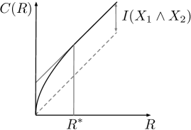
Figure 2: $C(R)$ as a function of $R$. $R^{\ast}$ denotes the point where $C(R)$ curve attains the slope $1$.

Corollary III.3.

For $R\geq 0$ and random variable $(X_{1},X_{2})$ taking values in a finite set ${\mathcal{X}}_{1}\times{\mathcal{X}}_{2}$, we have

$$C(R)=\left\{\begin{array}[]{ll}f(R)&\mbox{if }R\leq R^{*}\\ I(X_{1}\wedge X_{2})+R&\mbox{if }R>R^{*}\end{array}\right..$$

Another interesting point in the $C(R)$ curve is the slope at $R=0$, namely the amount of CR that can be generated per bit of communication. A related problem studied in [117, Proposition 2] gives a characterization of this quantity (with minor changes in the proof). If we restrict ourselves to $1$-round protocols, $i.e.$, the slope of $C_{1}(R)$ for $R=0$, it is given by $1/(1-s^{*}(X_{1},X_{2}))$ where $s^{*}(X_{1},X_{2})$ is defined in Section II-B.

III-B Communication for a fixed-length CR

The variant of the CR agreement problem that we describe in this section has been proposed recently, and the literature on it is thin in comparison with the classic formulation of the previous section. In fact, most of our treatment is based on a recent paper [84]. Nevertheless, the techniques used and the results are interesting. Furthermore, a comprehensive understanding of the CR problem requires a unified treatment that will yield both variants of the CR generation problem as special cases.

We are interested in the following quantity.

Definition III.3.

For jointly distributed random variables $(X_{1},X_{2})$, $c\geq 0$ is an $(\varepsilon,r)$-achievable communication length for CR of length $l$ if there exists an $r$-round private coin protocol $\pi$ of length less than $c$ and with outputs $(S_{1},S_{2})$ such that, for a random string $S$ distributed uniformly over $\{0,1\}^{l}$,

$${\mathrm{Pr}}\left(S_{1}=S_{2}=S\right)\geq 1-\varepsilon.$$

The infimum over all $(\varepsilon,r)$-achievable communication lengths for CR of length $l$ is denoted by $C_{\varepsilon,r}(l|X_{1},X_{2})$. Further, denote the infimum of $C_{\varepsilon,r}(l|X_{1},X_{2})$ over $r$ as $C_{\varepsilon}(l|X_{1},X_{2})$.

As in the previous section, we are interested in understanding the behavior of $C_{\varepsilon,r}(l|X_{1}^{n},X_{2}^{n})$ as a function of $l$ and $n$; the dependence on $r$ and $\varepsilon$ is also of interest, but perhaps more challenging to study. However, no general result characterizing the trade-off between the communication length, the CR length, and the number of samples $n$ is available. We shall focus on the limiting behavior as $n$ goes to infinity. This represents a fundamental trade-off between communication and CR lengths, regardless of the number of samples. In fact, we restrict ourselves to one round protocols and consider the following quantity:

$$\Gamma_{\varepsilon}(l)\mathbin{:=}\limsup_{n\rightarrow\infty}\,C_{\varepsilon,1}(l|X_{1}^{n},X_{2}^{n}).$$

We review a representative result of the treatment in [84] which focuses on a $BSS(\rho)$ . The notion of CR used in [84] is slightly different from the one we described above. In particular, the definition of CR in [84] requires that the estimate $S_{1}$ of ${\mathcal{P}}_{1}$ equals $S$ and replaces the uniformity of $S$ on $\{0,1\}^{l}$ with an alternative requirement of $H_{\tt min}(S_{1})\geq l$. The key technical difference is that this definition insists that one of the parties gets the exact CR $S$ (unlike our definition where both parties only obtained estimates of $S$). The following result of [84] applies to this restrictive notion of CR:

Theorem III.4.

Given $(X_{1},X_{2})$ generated by $BSS(\rho)$, $l>0$, and $\theta>0$, there exists $\varepsilon\leq 1-2^{-\theta l-{\mathcal{O}}(\log l)}$ such that

$$\Gamma_{\varepsilon}(l)\leq\big{(}(1-\rho^{2})(1-\theta)-2\rho\sqrt{(1-\rho^{2})\theta}\big{)}\cdot l.$$

Furthermore, for every $\varepsilon\leq 1-2^{-\theta l}$, it holds that

$$\Gamma_{\varepsilon}(l)\geq\big{(}(1-\rho^{2})(1-\theta)-2\rho\sqrt{(1-\rho^{2})\theta}\big{)}\cdot l.$$

Note that the result above focuses on very small probability of agreement and is uninteresting when $\varepsilon$ is required to be close to $0$. This regime is interesting for historical reasons. Specifically, the problem of generating CR without communicating goes back to the classic paper of Gács and Körner [75] which shows that (for indecomposable distributions) no positive rate of CR can be established without communicating, even when a fixed probability of error is allowed (see also [124] for an alternative proof). A companion result was shown by Witsenhausen [178] establishing that the parties cannot even agree on a single bit with non-vanishing (in observation length $n$) probability of agreement. An extension of this result appears in [33] (see [53] for further refinements) where it is shown that the largest probability with which the parties can agree on $\ell$ bits without communication is exponentially small in $\ell$ and the best exponent is established. Theorem III.4 is in a similar vein and shows that the two parties can agree on $\ell$ bits with exponentially small probability using $c\ell$ bits of communication where the constant $c$ depends on the exponent of the error. In fact, the scheme in [84] is related to [33] – both papers make the point that simple schemes where the CR is a subset of observed bits is suboptimal.

We remark that it is of interest to consider the problem of common randomness generation when no communication is allowed. We defer this discussion to Section V-C, where we consider the problem of generating correlated random variables without communicating. However, for comparison one can consider a simple scheme for the problem of this section where ${\mathcal{P}}_{1}$ and ${\mathcal{P}}_{2}$ simply declare their observed bits $X_{1}^{\ell}$ and $X_{2}^{\ell}$ as their respective estimates for CR. This scheme does not use any communication and yields $\varepsilon=1-(\frac{1}{2}(1-\rho))^{\ell}$.

Outline of achievability proof for Theorem III.4

The one-way communication scheme proposed in [84] is very similar to the one we reviewed in the previous section. Note that the typical set used in our scheme consists, in essence, of sequences which are correlated in the sense that they are jointly typical. However, since the focus here is on a simple BSS, a much simpler notion of correlation and typical sets can be used. In particular, we can make do with linear correlation. For simplicity, we assume that ${\mathcal{P}}_{1}$ and ${\mathcal{P}}_{2}$ observe $n$ iid samples $\{(X_{1i},X_{2i})\}_{i=1}^{n}$ from $\{-1,1\}$-valued $X_{1}$ and $X_{2}$ which have the same sign with probability $(1+\rho)/2$.

The CR generation protocol we describe below involves parameters $r>0,\eta>0$, and $c\in(0,1)$, which will be chosen later. Consider a random codebook comprising $2^{\ell}$ vectors $U^{n}(i,j)$, $1\leq i\leq 2^{c\ell}$ and $1\leq j\leq 2^{(1-c)\ell}$. The vectors $U^{n}(i,j)=(U_{1}(i,j),...,U_{n}(i,j))$ are iid for different $(i,j)$, each consisting of a uniformly generated vector from $\{-1,+1\}^{n}$. The protocol for CR generation is very similar to the one above:

1. ${\mathcal{P}}_{1}$ finds $\Pi_{1}$ which is the smallest $i$ for which there exists a $j$ such that the sequence $u^{n}=U^{n}(i,j)$ satisfies

   $$\langle X_{1}^{n}\,,\,u^{n}\rangle\mathbin{:=}\sum_{l=1}^{n}X_{1l}u_{l}\geq r\sqrt{n}.$$

   Denote by $Y_{1}$ the sequence $u^{n}$.

2. ${\mathcal{P}}_{1}$ sends $\Pi_{1}$ to ${\mathcal{P}}_{2}$.

3. ${\mathcal{P}}_{2}$ searches for the smallest index $j$ such that $v^{n}=U^{n}(\Pi_{1},j)$ satisfies $\langle X_{2}^{n},v^{n}\rangle\geq(1-\eta)r\sqrt{n}$. Denote by $Y_{2}$ the sequence $U^{n}(\Pi_{1},j)$.

The probability that $Y_{1}$ and $Y_{2}$ are the same is bounded below by the probability that the following hold:

• There exists $(i,j)$ such that for $u^{n}=U^{n}(i,j)$, $\langle X_{1}^{n}\,,\,u^{n}\rangle\geq r\sqrt{n}$ and $\langle X_{2}^{n}\,,\,u^{n}\rangle\geq(1-\eta)r\sqrt{n}$;

• for every other index pair $(i^{\prime},j^{\prime})$, $\langle X_{1}^{n}\,,\,U^{n}(i^{\prime},j^{\prime})\rangle<r\sqrt{n}$;

• for every other index $j^{\prime}$, $\langle X_{2}^{n}\,,\,U^{n}(i,j^{\prime})\rangle<(1-\eta)r\sqrt{n}$.

For sufficiently large $n$, we can approximate the random variables $\langle X_{1}^{n}\,,\,u^{n}\rangle$ and $\langle X_{2}^{n}\,,\,u^{n}\rangle$ with Gaussian random variables using the Bérry-Esséen theorem (cf. [73]). In particular, $\langle X_{1}^{n}\,,\,u^{n}\rangle$ can be approximated as a Gaussian random variable with mean $0$ and variance $n$. Therefore, ${\mathrm{Pr}}\left(\langle X_{1}^{n}\,,\,u^{n}\rangle\geq r\sqrt{n}\right)\approx Q(r)$, where $Q(x)={\mathrm{Pr}}\left(G>x\right)$ and $G$ is the standard Gaussian random variable. Furthermore, given a fixed realization $X_{1}^{n}=x_{1}^{n}$ such that $\langle x_{1}^{n}\,,\,u^{n}\rangle=r^{\prime}\sqrt{n}$ for some $r^{\prime}\geq r$, $\langle X_{2}^{n}\,,\,u^{n}\rangle$ can be approximated as a Gaussian random variable with mean $\rho r^{\prime}\sqrt{n}$ and variance $(1-\rho^{2})n$. Therefore,

$${\mathrm{Pr}}\left(\langle X_{2}^{n}\,,\,u^{n}\rangle\geq\eta r\sqrt{n}|X_{1}^{n}=x_{1}^{n}\right) \approx Q\left(\frac{\eta r-\rho r^{\prime}}{\sqrt{1-\rho^{2}}}\right)$$

$$\geq Q\left(\frac{(\eta-\rho)r}{\sqrt{1-\rho^{2}}}\right).$$

Thus, the probability of agreement can be seen to be bounded below roughly by

$$2^{\ell}Q(r)Q\left(\frac{(\eta-\rho)r}{\sqrt{1-\rho^{2}}}\right)(1-q_{2}-q_{3}),$$

where $q_{2}$ denotes the probability of event $(ii)$ above not happening given event $(i)$ and $q_{3}$ for event $(iii)$. Further, $q_{2}\leq 2^{\ell}Q(r)$ and $q_{3}\leq 2^{(1-c)\ell}Q((1-\eta)r)$. Also, note that for every fixed realization of the codebook, the probability that $Y_{1}$ equals $u^{n}=U^{n}(i,j)$ is bounded above by $Q(r)$ which yields $H_{\tt min}(Y_{1})\geq\ell$ upon choosing $Q(r)\approx 2^{-\ell}$. This fixes the value of $r$ as $\theta(\sqrt{\ell})$; the parameter $c$ is chosen as the minimum possible so that we can find some $\eta$ that yields the required probability of agreement.

Remark 3.

The scheme proposed in [84] uses a slightly different (structured) codebook construction, suggested in [33], which renders $Y_{1}$ uniformly distributed over $\{0,1\}^{\ell}$. Our alternative presentation above is aimed at pointing out the similarity between the scheme of [84] and the standard information theoretic approach used in [3].

Outline of converse proof for Theorem III.4

We have assumed that the CR $S$ equals $S_{1}$ and is a function, say $g$, of $X_{1}^{n}$, and $H_{\min}(g(X_{1}^{n}))\geq\ell$. The proof of lower bound we present remains valid for every $n$ by the tensorization property of hypercontractivity (cf. (5)); we fix $n=1$. For simplicity, we restrict ourselves to deterministic communication protocols $\pi$ of length $t$. For a fixed $x_{2}$ and different possible transcripts of the communication protocol, ${\mathcal{P}}_{2}$ can output different estimates for the CR; we denote this set of possible estimated CR values by ${\mathcal{Z}}_{x_{2}}$. Clearly, $|{\mathcal{Z}}_{x_{2}}|\leq 2^{t}$ for every $x_{2}\in{\mathcal{X}}_{2}$. It can be seen that

$$1-\varepsilon\leq{\mathbb{E}}\left[\sum_{z\in{\mathcal{Z}}_{X_{2}}}{\mathrm{Pr}}\left(g(X_{1})=z|X_{2}\right)\right].$$

Using Hölder’s inequality,

$$1-\varepsilon \leq\sum_{z}{\mathrm{Pr}}\left(z\in{\mathcal{Z}}_{X_{2}}\right)^{\frac{1}{p^{\prime}}}{\mathbb{E}}\left[{\mathrm{Pr}}\left(g(X_{1})=z|X_{2}\right)^{p}\right]^{1/p}$$

$$\leq\sum_{z}{\mathrm{Pr}}\left(z\in{\mathcal{Z}}_{X_{2}}\right)^{\frac{1}{p^{\prime}}}{\mathrm{Pr}}\left(g(X_{1})=z\right)^{\frac{1}{q}}$$

$$\leq 2^{-\frac{\ell}{q}}\sum_{z}{\mathrm{Pr}}\left(z\in{\mathcal{Z}}_{X_{2}}\right)^{\frac{1}{p^{\prime}}},$$

where the second inequality holds since $\mathrm{P}_{X_{1}X_{2}}$ is $(p,q)$-hypercontractive and the third by the assumptions that $H_{\tt min}(g(X_{1}))\geq\ell$. The sum on the right-side of the previous bound can be bounded further as

$$\sum_{z}{\mathrm{Pr}}\left(z\in{\mathcal{Z}}_{X_{2}}\right)^{\frac{1}{p^{\prime}}} \leq\left(\sum_{z}{\mathrm{Pr}}\left(z\in{\mathcal{Z}}_{X_{2}}\right)\right)^{\frac{1}{p^{\prime}}}|{\mathcal{Z}}|^{\frac{1}{p}}$$

$$={\mathbb{E}}\left[|Z_{X_{2}}|\right]^{\frac{1}{p^{\prime}}}|{\mathcal{Z}}|^{\frac{1}{p}}$$

$$\leq 2^{\frac{t}{p^{\prime}}+\frac{\ell}{p}}$$

where the first inequality uses Hölder’s inequality and the final uses $|{\mathcal{Z}}_{X_{2}}|\leq 2^{t}$. Finally, using the assumption $1-\varepsilon\geq 2^{-\theta\ell}$, together with the bounds above we get

$$t\geq\ell\cdot\left[\frac{p-q-\theta pq}{q(p-1)}\right].$$

Up to this point, our analysis applies to any distribution $\mathrm{P}_{X_{1}X_{2}}$. The best bound will be obtained by maximizing the previous lower bound for $t$ over all $(p,q)$ such that $\mathrm{P}_{X_{1}X_{2}}$ is $(p,q)$-hypercontractive. In general, this set of $(p,q)$ is not explicitly characterized. However, for our case of BSS, we can optimize over $(p,q)$ characterized in Theorem II.3 to get the stated result.

III-C Discussion

In spite of our understanding of the shape of $C(R)$ described above, several basic questions remain open. Specifically, it remains open if a finite round protocol can attain $C(R)$, $i.e.$, for a given $\mathrm{P}_{X_{1}X_{2}}$ and $r\in{\mathbbm{N}}$, is $C(R)=C_{r}(R)$? An interesting machinery for addressing such questions, which also exhibits its connection to hypercontractivity constants, has been developed recently in [117] (see, also, [123, 37]). In another direction, it is an important problem to investigate the dependency of CR rate on error $\varepsilon$. The first step toward this direction is to prove a strong converse, i.e., $C(R)=C_{\varepsilon}(R)$ for all $\varepsilon\in(0,1)$, where $C_{\varepsilon}(R)$ is the supremum of $C_{\varepsilon,r}(R)$ over $r\in{\mathbbm{N}}$. For $r=1$, the strong converse was proved in [115] by using the blowing-up lemma [60]. More recently, the strong converse for general $r\in{\mathbbm{N}}$ was proved by using a general recipe developed in [162]. Finer questions such as the second-order asymptotics of CR length in $n$ for a fixed allowed error $\varepsilon$ and bounds for $L_{\varepsilon,r}(c|X_{1},X_{2})$ are open; recently, a technique to derive the second-order converse bound using reverse hypercontractivity was developed in [118] (see also [113, Sec. 4.4.4]).

For the fixed-length CR case, the analysis for $BSS(\rho)$ presented above extends to $GSS(\rho)$ verbatim. But much remains open. For instance, the proof of the lower bound in [84] requires the nagging assumption that the CR is a function of only the observations of ${\mathcal{P}}_{1}$. It is easy to modify the proof to include local randomness, but it is unclear how to handle CR which depends on both $X_{1}^{n}$ and $X_{2}^{n}$. Perhaps a more interesting problem is the dependence of communication on the number of rounds; only a partial result is proved in [84] in this direction which shows that for binary symmetric sources interaction does not help if the CR is limited to a function of observation of one of the parties. Of course, the holy grail here is a complete trade-off between the communication length, the CR length, and the number of samples, which is far from understood. Some recent progress in this direction includes a sample efficient explicit scheme for CR generation in [78] and examples establishing lower bounds for number of round for fixed amount of communication per round in [12]. Yet several very basic questions remain open; perhaps the simplest to state is the following: Does interaction help to reduce communication for CR agreement for a binary symmetric source? An interested reader can see [117] for further discussion on this question.

The results we covered above were only for iid sources. We close this section with references to an interesting recent line of work [23, 21, 22] that extends the results of [75, 178] (a two-party extension of) the more general class of Santha-Vazirani sources (see [152].

IV Secret key agreement

We now introduce the secret key (SK) agreement problem which entails generating a CR that is independent of the communication used to generate it.

IV-A Secret keys using unlimited communication

We start with SK agreement when the amount of communication over the public channel is not restricted. Parties ${\mathcal{P}}_{1}$ and ${\mathcal{P}}_{2}$ observing $X_{1}$ and $X_{2}$, respectively, communicate over a noiseless public communication channel that is accessible by an eavesdropper, who additionally observes a random variable $Z$ such that the tuple $(X_{1},X_{2},Z)$ has a (known) distribution $\mathrm{P}_{X_{1}X_{2}Z}$.

The parties communicate using a private coin protocol $\pi$ to generate a CR $K$ taking values in ${\mathcal{K}}$ and with $K_{1}$ and $K_{2}$ denoting its estimates at ${\mathcal{P}}_{1}$ and ${\mathcal{P}}_{2}$, respectively. The CR $K$ constitutes an $(\varepsilon,\delta)$-SK of length $\log|{\mathcal{K}}|$ if it satisfies the following two conditions:

$$\Pr(K_{1}=K_{2}=K) \geq 1-\varepsilon,$$ (20)

$$d(\mathrm{P}_{K\Pi Z},\mathrm{P}_{\mathtt{unif}}\times\mathrm{P}_{\Pi Z}) \leq\delta,$$ (21)

where $\Pi$ denotes the random transcript of $\pi$ and $\mathrm{P}_{\mathtt{unif}}$ is the uniform distribution on ${\mathcal{K}}$. The first condition (20) guarantees the reliability of the SK and the second condition (21) guarantees secrecy.

Definition IV.1.

Given $\varepsilon,\delta\in[0,1)$, the supremum over the length $\log|{\mathcal{K}}|$ of $(\varepsilon,\delta)$-SK is denoted by $S_{\varepsilon,\delta}(X_{1},X_{2}|Z)$.

The only interesting case is when $\varepsilon+\delta<1$. In fact, when $\varepsilon+\delta\geq 1$, it can be shown that the parties can share arbitrarily long SK, i.e., $S_{\varepsilon,\delta}(X_{1},X_{2}|Z)=\infty$ [160, Remark 3].

Achievability techniques

Loosely speaking, the SK agreement schemes available in the literature can be divided into two steps: An information reconciliation step where the parties generate CR (which is not necessarily uniform or secure) using public communication; and a privacy amplification step where a SK independent of the observations of the eavesdropper, i.e $(Z,\Pi)$, is extracted from the CR.

In the CR generation problem of the previous section, the specific form of the randomness that the parties agreed on was not critical. In contrast, typical schemes for SK agreement generate CR comprising specific random variables such as $X_{1}$ or $(X_{1},X_{2})$. This gives us an analytic handle on the amount of randomness available for extracting the SK. Clearly, agreeing on $(X_{1},X_{2})$ makes available a larger amount of randomness for the parties to extract an SK. However, this will require a larger amount of public communication, thereby increasing the information leaked to the eavesdropper. To shed further light on this tradeoff, we review the details of the scheme where both parties agree on $X_{1}$ in the information reconciliation step.

In this case, ${\mathcal{P}}_{1}$ needs to send a message to ${\mathcal{P}}_{2}$ to enable the latter to recover $X_{1}$. This problem was studied first by Slepian and Wolf in their seminal work [154] where they characterized the optimal asymptotic rate required for the case where $(X_{1},X_{2}^{n})$ is iid. This asymptotic result can be recovered by setting $U=X_{1}$ and $V$ to be a constant in (9). In a single-shot setup, i.e., $n=1$, the Slepian-Wolf scheme can be described as follows: ${\mathcal{P}}_{1}$ sends the hash value $\Pi_{1}=F(X_{1})$ of observation $X_{1}$ where $F$ is generated uniformly from from a $2$-UHF. Then, ${\mathcal{P}}_{2}$ looks for a unique $x_{1}$ in a guess-list ${\cal L}_{x_{2}}\subseteq{\mathcal{X}}_{1}$ given $X_{2}=x_{2}$ that is compatible with the received message $\Pi_{1}$. A usual choice of the guess-list is the (conditionally) typical set: ${\cal T}_{\mathrm{P}_{X_{1}|X_{2}}}:=\{(x_{1},x_{2}):h_{\mathrm{P}_{X_{1}|X_{2}}}(x_{1}|x_{2})\leq t-\gamma\}$, where $h_{\mathrm{P}_{X_{1}|X_{2}}}(x_{1}|x_{2})=-\log\mathrm{P}_{X_{1}|X_{2}}\left(x_{1}|x_{2}\right)$ is the conditional entropy density, $t$ is the length of the message sent by ${\mathcal{P}}_{1}$ and $\gamma\geq 0$ is a slack parameter. In this case, the size of guess-list can be bounded as $|\{x_{1}:(x_{1},x_{2})\in{\cal T}_{\mathrm{P}_{X_{1}|X_{2}}}\}|\leq 2^{t-\gamma}$. Since ${\mathcal{P}}_{2}$’s recovery $\hat{X}_{1}$ may disagree with $X_{1}$ when $(X_{1},X_{2})$ is not included in the typical set or there exists $\hat{x}_{1}\neq X_{1}$ such that $(\hat{x}_{1},X_{2})\in{\cal T}_{\mathrm{P}_{X_{1}|X_{2}}}$ and $F(X_{1})=F(\hat{x}_{1})$, the error probability is bounded as (eg. see [86, Section 7.2] for details)

$$\Pr\bigg{(}X_{1}\neq\hat{X}_{1}\bigg{)}\leq\mathrm{P}_{X_{1}X_{2}}\left({\cal T}_{\mathrm{P}_{X_{1}|X_{2}}}^{c}\right)+2^{-\gamma}.$$

When the observations are iid, by the law of large numbers, the error probability converges to $0$ as long as the message rate is larger than the conditional entropy, i.e.,

$$t\geq n(H(X_{1}|X_{2})+\nu)$$ (22)

for some $\nu>0$.

Once the parties agree on $X_{1}$, the parties generate a SK from $X_{1}$ by using $2$-UHF. By an application of the leftover hash lemma with $X_{1}$ and $\Pi_{1}$ playing the role of $X$ and $V$ in Theorem II.1, a SK satisfying (21) can be generated as long as

$$\log|{\mathcal{K}}|\leq H^{(\delta-\eta)/2}_{\min}(\mathrm{P}_{X_{1}Z}|Z)-t-\log(1/4\eta^{2})$$

for some $0\leq\eta<\delta$. A common choice of smoothing is a truncated distribution

$$\tilde{\mathrm{P}}_{X_{1}Z}(x_{1},z)=\mathrm{P}_{X_{1}Z}\left(x_{1},z\right)\mathbf{1}\big{[}h_{\mathrm{P}_{X_{1}|Z}}(x_{1}|z)>r\big{]}$$

for some threshold $r$. Then, we have $H_{\min}(\tilde{\mathrm{P}}_{X_{1}Z}|Z)\geq r$. By adjusting the threshold $r$ so that $\tilde{\mathrm{P}}_{X_{1}Z}\in{\cal B}_{(\delta-\eta)/2}(\mathrm{P}_{X_{1}Z})$, we have

$$H^{(\delta-\eta)/2}_{\min}(\mathrm{P}_{X_{1}Z}|Z)$$

$$\geq\sup\big{\{}r:\Pr\big{(}h_{\mathrm{P}_{X_{1}|Z}}(X_{1}|Z)\leq r\big{)}\leq\delta-\eta\big{\}}.$$

When the observations are iid, by the law of large numbers, a secret key with vanishing security parameter $\delta$ can be generated as long as

$$\log|{\mathcal{K}}|\leq n(H(X_{1}|Z)-\nu)$$ (23)

for some $\nu>0$.

By combining the two bounds (22) and (23), for vanishing $\varepsilon,\delta$, we can conclude that $(\varepsilon,\delta)$-SK of length roughly $n[H(X_{1}|Z)-H(X_{1}|X_{2})]^{+}$ can be generated, where $[t]^{+}=\max\{t,0\}$.

Alternatively, the parties can agree on $(X_{1},X_{2})$ in the information reconciliation step. This is enabled by first communicating $X_{1}$ to ${\mathcal{P}}_{2}$ using the scheme outlined above and then $X_{2}$ to ${\mathcal{P}}_{1}$ using a standard Shannon-Fano code. For iid observations, this will require $n(H(X_{1}|X_{2})+H(X_{2}|X_{1}))$ bits of communication $(\Pi_{1},\Pi_{2})$. Furthermore, by using the leftover hash lemma with $(X_{1},X_{2})$ and $(\Pi_{1},\Pi_{2})$ playing the role of $X$ and $V$ in Theorem II.1, we will be able to extract a SK of length roughly $n[H(X_{1}X_{2}|Z)-H(X_{1}|X_{2})-H(X_{2}|X_{1})]^{+}$, which in general is not comparable with the rate attained in the previous scheme. However, when $Z$ is constant the two rates coincide. This observation was made first in [62] where the authors used the latter CR generation, termed attaining omniscience, for multiparty SK agreement. In fact, a remarkable result of [62] shows that, when $Z$ is constant, the omniscience leads to an optimal rate SK even in the multiparty setup with arbitrary number of parties.

Converse techniques

Moving now to the converse bounds, we begin with a simple bound based on Fano’s inequality. For special cases, this bound is asymptotically tight for iid observations, when $\varepsilon$ and $\delta$ vanish to $0$.

Theorem IV.1.

For every $0\leq\varepsilon,\delta<1$ with $0\leq\varepsilon+\delta<1$, it holds that

$$S_{\varepsilon,\delta}(X_{1},X_{2}|Z)\leq\frac{I(X_{1}\wedge X_{2}|Z)+h(\varepsilon)+h(\delta)}{1-\varepsilon-\delta}$$

The proof of Theorem IV.1 entails two steps. First, by using Fano’s inequality and the continuity of the Shannon entropy, an $(\varepsilon,\delta)$-SK with estimates $K_{1},K_{2}$ for ${\mathcal{P}}_{1},{\mathcal{P}}_{2}$, respectively, satisfies

$$\log|{\mathcal{K}}|\leq\frac{I(K_{1}\wedge K_{2}|Z,\Pi)+h(\varepsilon)+h(\delta)}{1-\varepsilon-\delta}.$$ (24)

The claimed bound then follows by using the monotonicity of correlation property of interactive communication (cf. (6)).

Next, we present a stronger converse bound which, in effect, replaces the multiplicative loss of $1/(1-\varepsilon-\delta)$ by an additive $\log 1/(1-\varepsilon-\delta)$. The bound relies on a quantity related to binary hypothesis testing; we review this basic problem first. For distributions $\mathrm{P}$ and $\mathrm{Q}$ on ${\mathcal{X}}$, a test is described by a (stochastic) mapping $\mathrm{T}:{\mathcal{X}}\to\{0,1\}$. Denote by $\mathrm{P}[T]$ and $\mathrm{Q}[T]$, respectively, the size of the test and the probability of missed detection, $i.e.$,

$$\mathrm{P}[\mathrm{T}] =\sum_{x}\mathrm{P}(x)\mathrm{T}(0|x),$$

$$\mathrm{Q}[\mathrm{T}] =\sum_{x}\mathrm{Q}(x)\mathrm{T}(0|x).$$

Of pertinence is the minimum probability of missed detection for tests of size greater than $1-\varepsilon$, $i.e.$,

$$\beta_{\varepsilon}(\mathrm{P},\mathrm{Q}):=\inf_{\mathrm{T}:\mathrm{P}[\mathrm{T}]\geq 1-\varepsilon}\mathrm{Q}[\mathrm{T}],$$

When $\mathrm{P}^{n}$ and $\mathrm{Q}^{n}$ are iid distributions, Stein’s lemma (cf. [60]) yields

$$\lim_{n\to\infty}-\frac{1}{n}\log\beta_{\varepsilon}(\mathrm{P}^{n},\mathrm{Q}^{n})=D(\mathrm{P}\|\mathrm{Q}),~{}\forall 0<\varepsilon<1.$$

The following upper bound for SK length from [159, 160] involves $\beta_{\varepsilon}$. Heuristically, it relates the length of SK to the difficulty in statistically distinguishing the distribution $\mathrm{P}_{X_{1}X_{2}Z}$ from a “useless” distribution in which the observations of the parties are independent when conditioned on the observations of the eavesdropper.

Theorem IV.2.

Given $0\leq\varepsilon,\delta<1$ and $0<\eta<1-\varepsilon-\delta$, it holds that

$$S_{\varepsilon,\delta}(X_{1},X_{2}|Z)$$

$$\leq-\log\beta_{\varepsilon+\delta+\eta}(\mathrm{P}_{X_{1}X_{2}Z},\mathrm{Q}_{X_{1}X_{2}Z})+2\log(1/\eta)$$

for any $\mathrm{Q}_{X_{1}X_{2}Z}$ satisfying $\mathrm{Q}_{X_{1}X_{2}Z}=\mathrm{Q}_{X_{1}|Z}\mathrm{Q}_{X_{2}|Z}\mathrm{Q}_{Z}$.

We outline the proof of Theorem IV.2. The first observation is that the reliability and secrecy conditions for an $(\varepsilon,\delta)$-SK impliy (and are roughly equivalent to) the following single condition:

$$d(\mathrm{P}_{K_{1}K_{2}Z\Pi},\mathrm{P}^{(2)}_{\mathtt{unif}}\times\mathrm{P}_{Z\Pi})\leq\varepsilon+\delta,$$ (25)

where

$$\mathrm{P}^{(2)}_{\mathtt{unif}}(k_{1},k_{2}):=\frac{{\mathds{1}}(k_{1}=k_{2})}{|{\mathcal{K}}|}.$$

Next, note that for a distribution $\mathrm{Q}_{X_{1}X_{2}Z}$ satisfying $\mathrm{Q}_{X_{1}X_{2}Z}=\mathrm{Q}_{X_{1}|Z}\mathrm{Q}_{X_{2}|Z}\mathrm{Q}_{Z}$, the property in (6) implies that the distribution $\mathrm{Q}_{K_{1}K_{2}Z\Pi}$ of the “view of the protocol” equals the product $\mathrm{Q}_{K_{1}|Z\Pi}\mathrm{Q}_{K_{2}|Z\Pi}\mathrm{Q}_{Z\Pi}$.

We will show that the two observations above yield the following bound: For any $(K_{1},K_{2})$ satisfying (25) and any $\mathrm{Q}_{K_{1}K_{2}Z\Pi}$ of the form $\mathrm{Q}_{K_{1}|Z\Pi}\mathrm{Q}_{K_{2}|Z\Pi}\mathrm{Q}_{Z\Pi}$, it holds that

$$\log|{\mathcal{K}}|\leq-\log\beta_{\varepsilon+\delta+\eta}(\mathrm{P}_{K_{1}K_{2}Z\Pi},\mathrm{Q}_{K_{1}K_{2}Z\Pi})+2\log(1/\eta).$$ (26)

The bound of Theorem IV.2 can be obtained by using the “data-processing inequality” for $\beta_{\varepsilon}(\mathrm{P}\circ W,\mathrm{Q}\circ W)\leq\beta_{\varepsilon}(\mathrm{P},\mathrm{Q})$, where $(\mathrm{P}\circ W)(y)=\sum_{x}\mathrm{P}(x)W(y|x)$.

For proving (26), we prove a reduction of independence testing to SK agreement. In particular, we use a given SK agreement protocol to construct a hypothesis test between $\mathrm{P}_{K_{1}K_{2}Z\Pi}$ and $\mathrm{Q}_{K_{1}K_{2}Z\Pi}$. The constructed test is a standard likelihood-ratio test, but instead of the likelihood ratio test between $\mathrm{P}_{K_{1}K_{2}Z\Pi}$ and $\mathrm{Q}_{K_{1}K_{2}Z\Pi}$, we consider the likelihood ratio of $\mathrm{P}^{(2)}_{\mathtt{unif}}\times\mathrm{P}_{Z\Pi}$ and $\mathrm{Q}_{K_{1}K_{2}Z\Pi}$. Specifically, the acceptance region for our test is given by

$${\cal A}:=\bigg{\{}(k_{1},k_{2},z,\tau):\log\frac{\mathrm{P}^{(2)}_{\mathtt{unif}}(k_{1},k_{2})}{\mathrm{Q}_{K_{1}K_{2}|Z\Pi}\left(k_{1},k_{2}|z,\tau\right)}\geq\lambda\bigg{\}},$$

where $\lambda=\log|{\cal K}|-2\log(1/\eta)$. Then, a change-of-measure argument of bounding probabilities under $\mathrm{Q}_{K_{1}K_{2}|Z\Pi}$ by those under $\mathrm{P}^{(2)}_{\mathtt{unif}}$ yields the following bound on the type II error probability:

$$\mathrm{Q}_{K_{1}K_{2}Z\Pi}\left({\cal A}\right)\leq\frac{1}{|{\mathcal{K}}|\eta^{2}}.$$

On the other hand, the security condition (cf. (25)) yields a bound on the type I error probability:

$$\mathrm{P}_{K_{1}K_{2}Z\Pi}\left({\cal A}^{c}\right)$$

$$\leq d(\mathrm{P}_{K_{1}K_{2}Z\Pi},\mathrm{P}^{(2)}_{\mathtt{unif}}\times\mathrm{P}_{Z\Pi})+\mathrm{P}^{(2)}_{\mathtt{unif}}\times\mathrm{P}_{Z\Pi}({\cal A}^{c})$$

$$\leq\varepsilon+\delta+\mathrm{P}^{(2)}_{\mathtt{unif}}\times\mathrm{P}_{Z\Pi}({\cal A}^{c}),$$

where the first inequality follows from the definition of the variational distance. For the second term, note that by the definition of the set ${\mathcal{A}}$ for any $(k,k,z,\tau)\in{\mathcal{A}}^{c}$

$$1\leq|{\mathcal{K}}|^{2}\eta^{2}\mathrm{Q}_{K_{1},K_{2}|Z\Pi}\left(k,k|z,\tau\right),$$

which yields

$$\sum_{(k_{1},k_{2}):(k_{1},k_{2},z,\tau)\in{\mathcal{A}}^{c}}\frac{{\mathds{1}}(k_{1}=k_{2})}{|{\mathcal{K}}|}$$

$$\leq\eta\sum_{k:(k,k,z,\tau)\in{\mathcal{A}}^{c}}\sqrt{\mathrm{Q}_{K_{1}K_{2}|Z\Pi}\left(k,k|z,\tau\right)}$$

$$\leq\eta\sqrt{\sum_{k}\mathrm{Q}_{K_{1}|Z\Pi}\left(k|z,\tau\right)\sum_{k}\mathrm{Q}_{K_{2}|Z\Pi}\left(k|z,\tau\right)}$$

$$=\eta,$$

where the last inequality uses the product form of $\mathrm{Q}_{K_{1}K_{2}|Z\Pi}$; (26) follows by combining the bounds above.

The proofs of the two converse bounds presented above follow roughly the same template: First, use the reliability and secrecy conditions to bound the length of an SK by a measure of correlation (see, for instance, (24) and (26)); and next, use properties of interactive communication and a data-processing inequality for the measure of correlation used to get the final bounds that entail only the original distribution. The monotone approach (cf. [48, 150, 80]) for proving converse bounds is an abstraction of these two steps. More specifically, the monotone approach seeks to identify measures of correlation that satisfy properties that enable the aforementioned bounds. This allows us to convert a problem of proving converse bounds to that of verifying these properties for appropriately chosen measures of correlation. The two bounds above, in essence, result upon choosing $I(X_{1}\wedge X_{2}|Z)$ and $\min_{\mathrm{Q}_{X_{1}X_{2}Z}}\beta_{\varepsilon}(\mathrm{P}_{X_{1}X_{2}Z},\mathrm{Q}_{X_{1}X_{2}Z})$ as those measures of correlation. This approach is used not only in the SK agreement analysis, but is also relevant in other related problems of “generating correlation” such as multiparty secure computation [179, 144] and entanglement distillation [69] in quantum information theory.

Secret key capacity

When the observations of the parties and the eavesdropper comprise an iid sequences $X_{1}^{n},X_{2}^{n},Z^{n}$, we are interested in examining how the maximum length of a SK that the parties can generate grows with $n$. The first order asymptotic term is the secret key capacity defined as

$$C^{\mathtt{sk}}_{\varepsilon,\delta}(X_{1},X_{2}|Z):=\liminf_{n\to\infty}\frac{1}{n}S_{\varepsilon,\delta}(X_{1}^{n},X_{2}^{n}|Z^{n})$$ (27)

and

$$C^{\mathtt{sk}}(X_{1},X_{2}|Z):=\lim_{\varepsilon,\delta\to 0}C^{\mathtt{sk}}_{\varepsilon,\delta}(X_{1},X_{2}|Z).$$ (28)

Evaluating the achievability bound derived above for iid observations, we get

$$C^{\mathtt{sk}}(X_{1},X_{2}|Z) \geq H(X_{1}|Z)-H(X_{1}|X_{2})$$ (29)

$$=I(X_{1}\wedge X_{2})-I(X_{1}\wedge Z).$$

For the converse bound, we can evaluate the single-shot result of Theorem IV.2 using Stein’s Lemma (cf. [60]) to obtain the following:

Theorem IV.3.

For $\varepsilon,\delta\in(0,1)$ with $\varepsilon+\delta<1$, we have

$$C^{\mathtt{sk}}_{\varepsilon,\delta}(X_{1},X_{2}|Z)\leq I(X_{1}\wedge X_{2}|Z).$$

The inequality holds with equality when $X_{1}$, $X_{2}$, and $Z$ form Markov chain in any order. In particular, when $Z$ is constant, the SK capacity is

$$C^{\mathtt{sk}}_{\varepsilon,\delta}(X_{1},X_{2})=I(X_{1}\wedge X_{2}).$$

The remarkable feature of this bound is that it holds for every fixed $0<\varepsilon,\delta$ such that $\varepsilon+\delta<1$. Note that if we used Theorem IV.1 in place of Theorem IV.2, we would have only obtained a matching bound when $\varepsilon$ and $\delta$ vanish to $0$, namely a weak converse result. Instead, using Theorem IV.2 leads to a characterization of capacity with a strong converse. When the Markov relation $X_{1}-\!\!\!\!\circ\!\!\!\!-X_{2}-\!\!\!\!\circ\!\!\!\!-Z$ holds, (29) and the identity $I(X_{1}\wedge X_{2}|Z)=H(X_{1}|Z)-H(X_{1}|X_{2})$ yield the claimed characterization of capacity. In such a case, Theorem IV.1 claims that the SK capacity does not depend on $\varepsilon$ and $\delta$ as long as $\varepsilon+\delta<1$. An interesting question is if $C^{\mathtt{sk}}_{\varepsilon,\delta}(X_{1},X_{2}|Z)$ only depends on $\varepsilon+\delta$ in general. In fact, a weaker claim can be proved: by using an argument to convert a high reliability protocol to a zero-secrecy protocol [95, Proposition 4], $C^{\mathtt{sk}}_{\varepsilon^{\prime},\delta^{\prime}}(X_{1},X_{2}|Z)\geq C^{\mathtt{sk}}_{\varepsilon,\delta}(X_{1},X_{2}|Z)$ holds as long as $\varepsilon^{\prime}\geq\varepsilon$ and $\varepsilon^{\prime}+\delta^{\prime}\geq\varepsilon+\delta$.

In general, a characterization of SK capacity is an open problem. It is also difficult to decide whether the SK capacity is positive or not, but there is a recent progress on this problem in [82]. In fact, it can be proved that the SK capacity is positive if and only if one-bit secret key with $\varepsilon+\delta<\frac{3-\sqrt{5}}{8}$ in (25) can be generated.

For the special case when we restrict ourselves to SK agreement protocols using one-round communication, say from ${\mathcal{P}}_{1}$ to ${\mathcal{P}}_{2}$, a characterization of SK capacity $C^{\mathtt{sk}}_{1}(X_{1},X_{2}|Z)$ was given in [2, Theorem 1].

Theorem IV.4.

For a pmf $\mathrm{P}_{X_{1}X_{2}Z}$,

$$C^{\mathtt{sk}}_{1}(X_{1},X_{2}|Z)=\max_{U,V}\big{[}I(V\wedge X_{2}|U)-I(V\wedge Z|U)\big{]},$$

where the maximum is taken over auxiliary random variables $(U,V)$ satisfying $U-\!\!\!\!\circ\!\!\!\!-V-\!\!\!\!\circ\!\!\!\!-X_{1}-\!\!\!\!\circ\!\!\!\!-(X_{2},Z)$. Moreover, it can be assumed that $V=(U,V^{\prime})$ and both $U$ and $V^{\prime}$ have range of size at most $|{\mathcal{X}}_{1}|$.

Returning to the general problem of unrestricted interactive protocols, we note that some improvements for the upper bound of Theorem IV.3 are known [127, 149, 80]. The following bound is roughly the state-of-the-art.

Theorem IV.5.

[80] For a pmf $\mathrm{P}_{X_{1}X_{2}Z}$,

$$C^{\mathtt{sk}}(X_{1},X_{2}|Z)\leq\inf\big{[}I(X_{1}\wedge X_{2}|U)+I(X_{1},X_{2}\wedge U|Z)\big{]},$$ (30)

where the infimum is taken over the conditional distributions $\mathrm{P}_{U|X_{1}X_{2}Z}$.

The bound of Theorem IV.5 is derived by an application of the monotone approach for proving converse bounds described earlier. A single-shot version of the asymptotic converse bound in Theorem IV.5 can be obtained using the bound in Theorem IV.2; see [160, Theorem 7] for details.

Moving to the achievability part, the lower bound of (29) is not tight and can be improved in general. In fact, even when the right-side of (29) is negative, a positive rate was shown to be possible in [126]. Interestingly, the scheme proposed in [126] uses interactive communication for information reconciliation, as opposed to one-way communication scheme that led to (29). This information reconciliation technique, termed “advantage distillation,” has been studied further in [127, 134, 135]. The best known lower bound for SK capacity appears in [80] which implies that

$$C^{\mathtt{sk}}(X_{1},X_{2}|Z)$$

$$\geq\sup_{\pi}{\tt IC}_{\tt e}(\pi|X_{1},X_{2})-{\tt IC}_{\tt i}(\pi|X_{1},X_{2})-I(\Pi\wedge Z)$$

where the supremum is over all private coin protocols $\pi$. Note that the form above is very similar to the one presented in Theorem III.2 and shows that the rate of the SK is obtained by subtracting from the rate of CR the rate of communication and the information leaked to the eavesdropper. In fact, the actual bound in [80], which we summarize below, is even stronger and allows us to condition on any initial part of the transcript, thereby recovering Theorem IV.4 as a special case.

Theorem IV.6.

For a pmf $\mathrm{P}_{X_{1}X_{2}Z}$,

$$C^{\mathtt{sk}}(X_{1},X_{2}|Z)$$

$$\geq\sup_{\pi}I(\Pi\wedge X_{1},X_{2}\mid\Pi^{t})-I(\Pi\wedge X_{1}|X_{2},\Pi^{t})$$

$$~{}~{}~{}-I(\Pi\wedge X_{2}|X_{1},\Pi^{t})-I(Z\wedge\Pi\mid\Pi^{t}),$$

where the supremum is over all private coin protocols $\pi$ and all $t$ less than $|\pi|$ and $\Pi^{t}$ denotes the transcript in the first $t$-rounds of communication.

The communication protocol attaining the bound above uses multiple rounds of interaction for information reconciliation. It was shown in [80] that the lower bound of Theorem IV.6 can strictly outperform the one-way SK capacity characterized in Theorem IV.4. However, the bound is not tight in general, even for binary symmetric sources [82].

Traditional notion of security used in the information theory literature is that of weak secrecy where information leakage is defined using mutual information normalized by block-length $n$ (see, for instance, [182, 126, 2]). In the past few decades, motivated by cryptography applications a more stringent notion of security with unnormalized mutual information, termed strong secrecy, has become popular. In fact, it turns out that the SK capacity under both notions of security coincide [128]. In this paper, we have employed the security definition with variational distance since it is commonly used in the cryptography literature and is consistent with other problems treated in this paper. In the i.i.d. setting, since the protocols reviewed above guarantee exponentially small secrecy in the variational distance, those protocols guarantee strong secrecy as well.

IV-B Secret key generation with communication constraint

In the previous section, there was no explicit constraint placed on the amount of public communication allowed. Of course, there is an implicit constraint implied by the secrecy condition. Nevertheless, not having an explicit constraint on communication facilitated schemes where the parties communicated as many bits as required to agree on $X_{1}$ or $(X_{1},X_{2})$ and accounted for the communication rate in the previous amplification step. We now consider a more demanding problem where the parties are required to generate a SK using private coin protocols $\pi$ of length $|\pi|$ no more than $c$.

Definition IV.2.

Given $\varepsilon,\delta\in[0,1)$ and $c>0$, the supremum over the length $\log|{\mathcal{K}}|$ of $(\varepsilon,\delta)$-SK that can be generated by a $r$-rounds protocol $\pi$ with $|\pi|\leq c$ is denoted by $S_{r,\varepsilon,\delta}(X_{1},X_{2}|Z;c)$.

Given a rate $R>0$, the rate-limited SK capacity is defined as follows:

$$C^{\mathtt{sk}}_{r,\varepsilon,\delta}(R):=\liminf_{n\to\infty}\frac{1}{n}S_{r,\varepsilon,\delta}(X_{1}^{n},X_{2}^{n}|Z^{n};nR)$$ (31)

and

$$C_{r}^{\mathtt{sk}}(R):=\lim_{\varepsilon,\delta\to 0}C^{\mathtt{sk}}_{r,\varepsilon,\delta}(R).$$ (32)

The problem of SK agreement using rate-limited communication was first studied in [61]. The general problem of characterizing $C^{\mathtt{sk}}_{r}(R)$ remains open. However, a complete characterization is available for two special cases: First, the rate-limited SK capacity $C^{\mathtt{sk}}_{1}(R)$ when we restrict ourselves to one-way communication protocols is known. Second, an exact expression for $C^{\mathtt{sk}}_{r}(R)$ is known when $Z$ is constant (cf. [157, 117]). Specifically, for the rate-limited SK capacity with one-way communication, the following result holds.

Theorem IV.7 ([61]).

The rate-limited SK capacity using one-way communication protocols is given by

$$C^{\mathtt{sk}}_{1}(R)=\max_{U,V}\big{[}I(V\wedge X_{2}|U)-I(V\wedge Z|U)\big{]},$$

where the maximization is taken over auxiliary random variables $(U,V)$ satisfying $U-\!\!\!\!\circ\!\!\!\!-V-\!\!\!\!\circ\!\!\!\!-X_{1}-\!\!\!\!\circ\!\!\!\!-(X_{2},Z)$ and

$$I(V\wedge X_{1}|U)-I(V\wedge X_{2}|U)\leq R.$$

Moreover, it may be assumed that $V=(U,V^{\prime})$ and both $U$ and $V^{\prime}$ have range of size at most $|{\mathcal{X}}_{1}|+1$.

Theorem IV.7 has the same expression as Theorem IV.4 except that there is additional communication rate constraint. Because of this additional constraint, unlike the Slepian-Wolf coding used in the proof of Theorem IV.4, we need to use quantize-and-binning scheme à la the Wyner-Ziv coding.

In general, the expression in Theorem IV.7 involves two auxiliary random variables and is difficult to compute. However, explicit formulae are available for the specific cases of Gaussian sources and binary sources [172, 56, 116].

When the adversary’s observation $Z$ is constant, the SK agreement is closely related to the CR generation problem studied earlier. Heuristically, if the communication used to generate a SK is as small as possible, it is almost uniform, and therefore, $L_{\varepsilon}(c|X_{1},X_{2})\gtrsim S_{r,\varepsilon,\delta}(X_{1},X_{2}|Z;c)+c$. On the other hand, using the leftover hash lemma we can show the following.

Proposition IV.8.

Given $\varepsilon,\delta\in[0,1)$ and $c>0$, we have

$$S_{r,\varepsilon,\delta}(X_{1},X_{2}|Z;c)\geq L_{\varepsilon}(c|X_{1},X_{2})-c-2\log(1/2\delta)-1.$$

Using these observations and Theorem III.2, we get the following characterization of rate-limited SK capacity.

Theorem IV.9.

For $R>0$ and finite-valued $(X_{1},X_{2})$,

$$C^{\tt SK}_{r}(R)=\sup{{\tt IC}_{\tt e}(\pi|X_{1},X_{2})-{\tt IC}_{\tt i}(\pi|X_{1},X_{2})},$$

where the supremum is over all $r$-round private coin protocols $\pi$ such that ${\tt IC}_{\tt i}(\pi|X_{1},X_{2})\leq R$.

In fact, it can be seen that $C_{r}^{\tt sk}(R)$ is $R$ less than the maximum rate of CR that can be generated using $r$-round communication protocols of rate less than $R$. Thus, the optimal rate of an SK that can be generated corresponds to the difference between the $C(R)$ curve and the slope $1$ line in Figure 2. Since the maximum possible rate of SK is $I(X_{1}\wedge X_{2})$, the quantity $R^{*}$ depicted in Figure 2 corresponds to the minimum rate of communication needed to generate a SK of rate equal to $I(X_{1}\wedge X_{2})$. This minimum rate was studied first in [157] where a characterization of $R^{*}$ was given. Furthermore, an example was provided where $R^{*}$ cannot be attained by simple (noninteractive) protocols, which in turn constitutes an example where two parties can generate a SK of rate $I(X_{1}\wedge X_{2})$ without agreeing on $X_{1}$ or $X_{2}$ or $(X_{1},X_{2})$.

IV-C Discussion

Several basic problems remain open in spite of decades of work in this area. Perhaps most importantly, a characterization of SK capacity $C^{\tt sk}(X_{1},X_{2}|Z)$ is open in general. As we pointed out, it is known that interaction is needed in general to attain this capacity. Even when $Z$ is a constant, although interaction is not needed to attain the SK capacity, we saw that it can help reduce the rate of communication needed to generate an optimal rate SK. In another direction, [95] studied the second-order asymptotic term in $S_{\varepsilon,\delta}(X_{1}^{n},X_{2}^{n}|Z^{n})$ and used an interactive scheme with $O(n^{1/4})$ rounds of interaction to attain the optimal term when the Markov relation $X_{1}-\!\!\!\!\circ\!\!\!\!-X_{2}-\!\!\!\!\circ\!\!\!\!-Z$ holds. It remains open if a noninteractive protocol can attain the optimal second-order term. One of the difficulties in quantifying the performance of noninteractive protocols is that the converse bound of Theorem IV.2 allows arbitrary interactive communication and a general bound which takes the number of rounds of interaction into account is unavailable. Recently, [161] provided a universal protocol for generating an SK at rate within a ${\mathcal{O}}(\sqrt{n\log n})$ gap to the SK capacity without knowing the distribution $\mathrm{P}_{X_{1}X_{2}}$. Moreover, this protocol is interactive and uses $O(\sqrt{n})$ rounds of interaction. Studying the role of interaction in SK agreement is an interesting research direction. A noteworthy recent work in this direction is [117] where a connection between the expression for rate-limited SK capacity and an extension of the notion of hypercontractivity is used to study the benefit of interaction for SK agreement.

Another refinement that has received attention is the exponential decay rate for secrecy parameter $\delta$ and the decay exponent for error parameter $\varepsilon$. Bounds for achievable error exponents were given in [62] and follow from the classic error exponents for Slepian-Wolf coding (cf. [60]). An exponential decay rate for $\delta$ was also reported in [62] and further refinements can be obtained using exponential-leakage refinements for the leftover hash lemma from, for instance, [92, 93]. All these works consider error and secrecy exponents in isolation, and the problem of characterizing exponents for secret key agreement is open.

Also, while our treatment has focused on a simple source model, several extensions to other multiterminal source models where one or more terminals act as helpers have been studied starting with [61]. We have not included a review of this and other related setting including channel models for SK agreement (cf. [2, 63, 50, 51, 81, 51, 52, 64, 158]). Some of these topics and references to related literature can be found in the monograph [137].

A variant of the two-party SK agreement problem reviewed in this section has been studied in the computer science literature under the name of “fuzzy extractors,” starting from [68]. Unlike our setup above, in the fuzzy extractors model, the exact distribution of the observations $(X_{1},X_{2})$ is not fixed. Specifically, ${\mathcal{P}}_{1}$ observes a $k$-source $X_{1}$, $i.e.$, a source that has min-entropy at least $k$, and ${\mathcal{P}}_{2}$ observes $X_{2}$ such that the Hamming distance between $X_{1}$ and $X_{2}$ is less than a threshold with probability $1$. This is a two-party extension of the classic model of randomness extraction introduced in [55]. Although this direction of research has developed independently of the one in the information theory community, the techniques used are related; for instance, see [95, 74]. Note that the universal setting of [161] constitutes another variant of the problem where the distribution of the observations is unknown. However, the protocols proposed are theoretical constructs and, typically, the work on fuzzy extractors seeks computationally tractable protocols.

V Simulation without communication

In this section, we address the distributed simulation (or generation) of samples from a specified distribution by using samples from another distribution, but without communicating. We begin with a classic problem of Wyner where two parties seek to generate samples from a distribution using shared randomness. Instead of providing the original treatment of this problem from [180], we recover the known results using the more powerful framework of approximation of output statistics (AOS) introduced in [87]. The latter is reviewed first. We then proceed to the general problem of simulation, and close with an important “distributed information structure” variant where each party has only partial information about the distribution to be simulated. In the following section, we consider variants of simulation problems where communication is allowed; results of this section will serve as basic tools for the setting with communication.

V-A Approximation of output statistics

A standard simulation step in several applications entails generation of a given random variable using samples from a uniform distribution. The AOS problem is an extension where we seek to generate a given distribution as the output of a noisy channel using a uniform distribution on a subset of its input. A version of this problem was originally introduced in [180] as a tool to prove the achievability part of “Wyner common information,” which will be discussed in the next section. The general formulation, also referred to as the channel resolvability problem, was introduced in [87] in part as a tool to prove the converse for the identification capacity theorem [4]. More recently, it has been used as a tool for proving the achievability part of the reverse Shannon theorem (which we will review in Section VI-A) and the wiretap channel capacity [182] (cf. [58, 45, 91, 32]). In the information theory literature, the AOS problem has emerged as a basic building block for enabling distributed simulation.

For a given input distribution $\mathrm{P}_{X}$ and channel $W(y|x)$, our goal in the AOS problem is to simulate a given output distribution

$$\mathrm{P}_{Y}\left(y\right):=\sum_{x}\mathrm{P}_{X}\left(x\right)W(y|x).$$

To that end, we construct a code ${\mathcal{C}}=\{x_{1},\ldots,x_{|{\mathcal{C}}|}\}$ so that the output distribution

$$\mathrm{P}_{{\mathcal{C}}}\left(y\right):=\sum_{x\in{\mathcal{C}}}\frac{1}{|{\mathcal{C}}|}W(y|x)$$

corresponding to a uniform distribution over the codewords approximates the target output distribution $\mathrm{P}_{Y}$. For a given size $|{\mathcal{C}}|$ of input randomness, we seek to make the approximation error as small as possible. Various measures of “distance” have been used in the literature to evaluate the approximation error: for instance, Kullback-Leibler divergence, normalized Kullback-Leibler divergence, and the variational distance. In our treatment here, we use variational distance to measure error and denote $\rho({\mathcal{C}},\mathrm{P}_{Y}):=d(\mathrm{P}_{{\mathcal{C}}},\mathrm{P}_{Y})$.

Definition V.1.

For a given $\varepsilon\in[0,1)$, the infimum over the length $\log|{\mathcal{C}}|$ of AOS codes satisfying $\rho({\mathcal{C}},\mathrm{P}_{Y})\leq\varepsilon$ is denoted by $L_{\varepsilon}(\mathrm{P}_{X},W)$.

When the input distribution is iid $\mathrm{P}_{X}^{n}$ and the channel $W^{n}=\prod_{t=1}^{n}W$ is discrete memoryless, we consider the asymptotic limits defined by

$$C^{\mathtt{AOS}}_{\varepsilon}(\mathrm{P}_{X},W):=\limsup_{n\to\infty}\frac{1}{n}L_{\varepsilon}(\mathrm{P}_{X}^{n},W^{n})$$

and

$$C^{\mathtt{AOS}}(\mathrm{P}_{X},W):=\lim_{\varepsilon\to 0}C_{\varepsilon}(\mathrm{P}_{X},W).$$

Theorem V.1.

[180, 87, 88, 99, 169] For a given $\varepsilon\in(0,1)$, we have

$$C^{\mathtt{AOS}}_{\varepsilon}(\mathrm{P}_{X},W)=C^{\mathtt{AOS}}(\mathrm{P}_{X},W)=\min_{\mathrm{P}_{\tilde{X}}}I(\tilde{X}\wedge\tilde{Y}),$$ (33)

where the minimum is taken over all input distribution $\mathrm{P}_{\tilde{X}}$ such that the output distribution $\mathrm{P}_{\tilde{Y}}\left(y\right)=\sum_{x}\mathrm{P}_{\tilde{X}}\left(x\right)W(y|x)$ coincides with the target output distribution $\mathrm{P}_{Y}=\mathrm{P}_{X}\circ W$.

In [87], the motivation to introduce the AOS problem was to show the (strong) converse part of the identification capacity theorem [4]. For that purpose, it is useful to consider the worst-case with respect to input distributions:

$$C^{\mathtt{AOS}}_{\varepsilon}(W):=\limsup_{n\to\infty}\sup_{\mathrm{P}_{X^{n}}}\frac{1}{n}L_{\varepsilon}(\mathrm{P}_{X^{n}},W^{n})$$ (34)

and

$$C^{\mathtt{AOS}}(W):=\lim_{\varepsilon\to 0}C^{\mathtt{AOS}}_{\varepsilon}(W),$$

where the supremum in (34) is taken over all input distribution $\mathrm{P}_{X^{n}}$ that are not necessarily iid (the output distribution we are trying to approximate are given by $\mathrm{P}_{X^{n}}\circ W^{n}$). Interestingly, this worst-case quantity coincides with Shannon’s channel capacity.

Theorem V.2 ([87]).

For a given $\varepsilon\in(0,1)$, we have

$$C^{\mathtt{AOS}}_{\varepsilon}(W)=C^{\mathtt{AOS}}(W)=\max_{\mathrm{P}_{X}}I(X\wedge Y).$$ (35)

Even though the worst case AOS is characterized by the maximization of the single-letter input distribution in (35), the worst input distribution attaining the supremum in (34) may not be iid in general (see [87, Example 1]).

We outline the achievability proof of Theorem V.1. For simplicity, we assume $\mathrm{P}_{X}$ itself is the optimal distribution attaining the minimum in (33). To construct an AOS code, we randomly generate codewords ${\cal C}_{n}=\{\mathbf{x}_{1},\ldots,\mathbf{x}_{|{\cal C}_{n}|}\}$ according to $\mathrm{P}_{X}^{n}$. Then, the approximation error $\rho(\mathrm{P}_{{\cal C}_{n}},\mathrm{P}_{Y}^{n})$ averaged over the random choice of the code ${\cal C}_{n}$ can be evaluated by techniques from [87, 91, 139, 65]. Specifically, if the rate $\frac{1}{n}\log|{\cal C}_{n}|$ of the constructed AOS code is larger than $I(X\wedge Y)$, the convergence of the approximation error is guaranteed. A technical tool involved is a bound for the resulting approximation error; such results have been aptly named soft covering lemmas starting from [65]. The traditional covering lemma, proved using combinatorial arguments in [60], claims that the typical set of size $2^{nH(Y)}$ in the output space can be covered by almost disjoint “balls” of size $2^{nH(Y|X)}$ each centered around $2^{nI(X\wedge Y)}$ codewords. Interestingly, the soft covering lemma claims that the same number of codewords suffice to cover the output space in the sense of approximating the output distribution of a channel.

Originally, a version of the soft covering lemma was proved in [87]. Later, alternative versions appeared in [91, Theorem 2] and [139, Lemma 3]; a general version of the lemma can be found in [65, Theorem 7.1]. The proofs in [91, 139, 65] are all based on a similar strategy using the Cauchy-Schwarz inequality to bound the variational distance ($\ell_{1}$-distance) in terms of the $\ell_{2}$-distance, which is reminiscent of the proof of the leftover hash lemma.

The AOS problem has been extended in various directions. In fact, [87] studied the AOS problem for general channels that may not be stationary or ergodic. The convergence speed (exponent) of the approximation error was studied in [91, 139] and a complete characterization for the random coding exponent was derived in [143] (see, also, [YagCuf19]) . The second-order asymptotic rate for this problem was characterized in [169] under additional assumptions. A general formula for the leading asymptotic term in the optimal length of AOS codes for general channels and general input distributions was characterized recently in [184].

V-B Wyner common information

In an attempt to define an operational notion of common information of two random variables, Wyner studied the amount of shared uniform randomness needed for two parties to generate $n$ independent samples from a given joint distribution $\mathrm{P}_{X_{1}X_{2}}$. The number of shared random bits needed per sample is termed Wyner common information [180].

Formally, ${\mathcal{P}}_{1}$ and ${\mathcal{P}}_{2}$ have access to shared randomness $U$ distributed uniformly over a set ${\mathcal{U}}$ (constituting public coins) and unlimited private randomness $U_{1}$ and $U_{2}$ (constituting private coins), respectively. They seek to generate a sample from a fixed distribution $\mathrm{P}_{X_{1}X_{2}}$. To that end, they execute a simulation protocol comprising channels $W_{1}(\cdot|u)$ and $W_{2}(\cdot|u)$ with a common input alphabet ${\mathcal{U}}$. The output distribution of the protocol is given by

$$\mathrm{P}_{{\mathcal{C}}}(x_{1},x_{2})=\sum_{u\in{\mathcal{U}}}\frac{1}{|{\mathcal{U}}|}W_{1}(x_{1}|u)W_{2}(x_{2}|u),$$ (36)

and the corresponding simulation error by

$$\rho({\mathcal{C}},\mathrm{P}_{X_{1}X_{2}})=d(\mathrm{P}_{{\mathcal{C}}},\mathrm{P}_{X_{1}X_{2}}).$$

Definition V.2.

For a given $\varepsilon\in[0,1)$, the infimum over the length $\log|{\mathcal{U}}|$ of simulation protocols satisfying $\rho({\mathcal{C}},\mathrm{P}_{X_{1}X_{2}})\leq\varepsilon$ is denoted by $L_{\varepsilon}(\mathrm{P}_{X_{1}X_{2}})$.

For iid distribution $\mathrm{P}_{X_{1}X_{2}}^{n}$, the Wyner common information of $(X_{1},X_{2})$ is defined as follows:

$$C_{\varepsilon}^{\mathtt{Wyn}}(X_{1},X_{2}):=\limsup_{n\to\infty}\frac{1}{n}L_{\varepsilon}(\mathrm{P}_{X_{1}X_{2}}^{n})$$

and

$$C^{\mathtt{Wyn}}({X_{1}X_{2}}):=\lim_{\varepsilon\to 0}C_{\varepsilon}^{\mathtt{Wyn}}(\mathrm{P}_{X_{1}X_{2}}).$$

A single-letter expression for Wyner common information $C^{\tt Wyn}(X_{1},X_{2})$ was given in [180]; a strong converse establishing $C_{\varepsilon}^{\tt Wyn}(X_{1},X_{2})=C^{\tt Wyn}(X_{1},X_{2})$ for all $0<\varepsilon<1$ has been claimed recently in [192]. We summarize both results below.

Theorem V.3.

[180, 192] For a given $\varepsilon\in(0,1)$, we have

$$C_{\varepsilon}^{\mathtt{Wyn}}(X_{1},X_{2})=C^{\mathtt{Wyn}}({X_{1},X_{2}})=\min I(V\wedge X_{1},X_{2}),$$ (37)

where the minimization is taken over all auxiliary random variable $V$ satisfying $X_{1}-\!\!\!\!\circ\!\!\!\!-V-\!\!\!\!\circ\!\!\!\!-X_{2}$. Moreover, the range of $V$ may be assumed to be $|{\mathcal{V}}|\leq|{\mathcal{X}}_{1}||{\mathcal{X}}_{2}|$.

This problem is closely related to the AOS problem considered in the previous section. In fact, to prove the achievability part of Theorem V.3, we construct an AOS code as follows. For the optimal joint distribution $\mathrm{P}_{VX_{1}X_{2}}$ attaining the minimum in (37), note that the distribution $\mathrm{P}_{X_{1}X_{2}|V}$ can be factorized as $\mathrm{P}_{X_{1}|V}\times\mathrm{P}_{X_{2}|V}$ using the Markov chain condition. Thus, if we have an AOS code that approximates the output distribution $\mathrm{P}^{n}_{X_{1}X_{2}}$, which is the output distribution of channel $\mathrm{P}^{n}_{X_{1}X_{2}|V}$ with input distribution $\mathrm{P}^{n}_{V}$, then the parties can simulate $\mathrm{P}^{n}_{X_{1}X_{2}}$ by using the AOS code as shared randomness and $\mathrm{P}_{X_{1}|V}^{n}$ and $\mathrm{P}^{n}_{X_{2}|V}$ as local channels for the simulation protocol, respectively.

In the problem formulation above, we studied the worst-case length of common randomness required for generating the target joint distribution with vanishing error. Alternatively, we can consider the expected length of common randomness required to generate the target joint distribution exactly. Such a variant of the problem, termed exact common information, was studied in [109] (see also [111] for a protocol that exactly generates target distributions on continuous alphabets). The exact common information is larger than or equal to the Wyner common information by definition. For some sources such as the binary double symmetric source, it is known that the former is strictly larger than the latter [191].

V-C Simulation of correlated random variables

One important special case of the CR capacity result given in Theorem III.2 is when the rate of communication $R=0$. By Theorem III.2, this is given by the supremum of $I(U\wedge X_{1})$ such that the Markov relations $U-\!\!\!\!\circ\!\!\!\!-X_{1}-\!\!\!\!\circ\!\!\!\!-X_{2}$ and $U-\!\!\!\!\circ\!\!\!\!-X_{2}-\!\!\!\!\circ\!\!\!\!-X_{1}$ hold. This double Markov condition enforces $U$ to be a common function of $X_{1}$ and $X_{2}$, namely a $U$ such that $H(U|X_{1})=H(U|X_{2})=0$; $e.g.$ see [60, Problem 16.25] and [61, Lemma 1.1] for a slight sharpening of this result. The maximum of such common functions is referred to as the Gács-Körner common information of $(X_{1},X_{2})$, denoted $GK(X_{1},X_{2})$ [75]. Gács and Körner showed in [75] that the maximum rate of CR that two parties observing iid samples from $\mathrm{P}_{X_{1}X_{2}}$ can generate without communicating is $GK(X_{1},X_{2})$. In fact, when $GK(X_{1},X_{2})=0$ and no communication is allowed, Witsenhausen [178] showed that parties cannot even agree on a single unbiased bit.

In this section, we are interested in a generalization of this question: When can parties observing $(X_{1},X_{2})$ generate a single sample from a given distribution $\mathrm{Q}_{U_{1}U_{2}}$ with ${\mathcal{P}}_{1}$ getting $U_{1}$ and ${\mathcal{P}}_{2}$ getting $U_{2}$. Formally, we consider the following problem.

Definition V.3 (Simulation without communication).

Given distributions $\mathrm{P}_{X_{1}X_{2}}$ and $\mathrm{Q}_{U_{1}U_{2}}$, we say that $\mathrm{P}_{X_{1}X_{2}}$ can simulate $\mathrm{Q}_{U_{1}U_{2}}$ if for every $\varepsilon>0$ there exists $n\geq 1$ and functions $f:{\mathcal{X}}_{1}^{n}\to{\mathcal{U}}_{1}$ and $g:{\mathcal{X}}_{2}^{n}\to{\mathcal{U}}_{2}$ such that $d\left(\mathrm{P}_{f(X_{1}^{n})g(X_{2}^{n})},\mathrm{Q}_{U_{1}U_{2}}\right)\leq\varepsilon$. Denote by ${\mathcal{S}}(\mathrm{P}_{X_{1}X_{2}})$ the set of all distributions $\mathrm{Q}_{U_{1}U_{2}}$ such that $\mathrm{P}_{X_{1}X_{2}}$ can simulate $\mathrm{Q}_{U_{1}U_{2}}$.

While private randomness is not allowed in our formulation, it can easily be extracted using samples from $\mathrm{P}_{X_{1}X_{2}}$. Note that the common randomness generation problem and the Wyner common information, respectively, entail simulating a uniformly distributed shared bits from a given distribution and vice-versa. Also, a related setting where we seek to simulate a given channel using an available channel was considered in [85]. We do not review this problem here and restrict ourselves to the simple source model setting above.

An elemental question is to characterize the set ${\mathcal{S}}(\mathrm{P}_{X_{1}X_{2}})$. Surprisingly, this basic question was formulated only recently in [9] (see, also, [10]). However, several important instances of this general question appear in the information theory literature and the treatment of randomness in the computer science literature. In particular, the following result was shown in [178]:

Theorem V.4.

Every distribution $\mathrm{P}_{X_{1},X_{2}}$ can simulate $BSS(\rho)$ if

$$\rho\leq\frac{2}{\pi}\cdot\arcsin(\rho_{m}(X_{1},X_{2})).$$

The proof is simple and entails first simulating correlated Gaussian random variables with correlation $\rho_{m}(X_{1},X_{2})$ (using the central limit theorem) and then declaring their signs. A result of Borell [35] shows that for jointly Gaussian vectors $\mathrm{P}_{X_{1},X_{2}}$, the maximum of $\rho_{m}(f_{1}(X_{1}),f_{2}(X_{2}))$ over binary-valued $f_{1},f_{2}$ is obtained when $f_{1}$ and $f_{2}$ correspond to half-planes, namely they have the form $f_{i}(x)=\mathrm{sign}(a_{i}\cdot(x-b_{i}))$. As a corollary of this result (applied to $X_{1}^{n},X_{2}^{n}$) and the theorem above, we obtain the following.

Corollary V.5.

For jointly Gaussian $(X_{1},X_{2})$ with zero mean and covariance matrix

$$\begin{bmatrix}1&\rho_{0}\\ \rho_{0}&1\end{bmatrix},$$

$\mathrm{P}_{X_{1}X_{2}}$ can simulate $BSS(\rho)$ iff $\rho\leq\frac{2}{\pi}\cdot arcsin(\rho_{0})$.

The previous result gives precise conditions for $BSS(\rho)$ to be contained in ${\mathcal{S}}(GSS(\rho))$. The characterization of the set ${\mathcal{S}}(GSS(\rho))$, and in general of ${\mathcal{S}}(\mathrm{P}_{X_{1}X_{2}})$ for a general distribution $\mathrm{P}_{X_{1}X_{2}}$, is open. Partial results are available in [10] which provide general necessary conditions for a distribution to lie in ${\mathcal{S}}(\mathrm{P}_{X_{1}X_{2}})$. We review this result below, in a slightly different form, where a measure of correlation is used to capture the relation $\mathrm{Q}_{X_{1}X_{2}}\in{\mathcal{S}}(\mathrm{P}_{X_{1}X_{2}})$. Instead of specifying a measure of correlation, the next result provides a general characterization of such measures of correlation which behave monotonically along the containment relation (this approach is similar to that of monotones used in [150, 80, 81]).

Theorem V.6.

Consider a function $\Gamma(X,Y)$ satisfying the following properties:

1. Data processing inequality. $\Gamma(f(X),g(Y))\leq\Gamma(X,Y)$ for all functions $f,g$;

2. Tensorization property. $\Gamma(X^{n},Y^{n})=\Gamma(X_{1},Y_{1})$ for iid $(X^{n},Y^{n})$;

3. Lower semicontinuity. $\Gamma(X,Y)$ is a lower semicontinuous function of $\mathrm{P}_{XY}$.

If $\mathrm{P}_{X_{1}X_{2}}$ can simulate $\mathrm{Q}_{U_{1},U_{2}}$, then $\Gamma(U_{1},U_{2})\leq\Gamma(X_{1},X_{2})$.

As was pointed-out in [10], both $\rho_{m}(X,Y)$ and $s^{*}(X,Y)$ satisfy the conditions required of $\Gamma$ in Theorem V.6. We note that a more general class of measures of correlation satisfying these conditions is available [24] (see, also, [19]). As a corollary, we have the following.

Corollary V.7.

$BSS(\rho_{1})$ can simulate $BSS(\rho_{2})$ iff $\rho_{1}\geq\rho_{2}$.

Next, we review a few simple properties of ${\mathcal{S}}(\mathrm{P}_{X_{1}X_{2}})$ which have not been reported in literature, but perhaps are well-known. Clearly, the set ${\mathcal{S}}(\mathrm{P}_{X_{1}X_{2}})$ is closed. We note that the simulation induces a partial order on the set of distributions. Specifically, denoting by $\mathrm{P}_{X_{1}X_{2}}\succeq\mathrm{Q}_{U_{1}U_{2}}$ the relation “$\mathrm{P}_{X_{1}X_{2}}$ can simulate $\mathrm{Q}_{U_{1}U_{2}}$,” it can be shown that $\succeq$ is a preorder. Furthermore, define an equivalence relation $\mathrm{P}\sim\mathrm{Q}$ iff $\mathrm{P}\succeq\mathrm{Q}$ and $\mathrm{Q}\succeq\mathrm{P}$, and consider the set of equivalence classes $[\mathrm{P}]$. Then, the set of equivalence classes is a poset under the partial order induced by the preorder $\succeq$. It is easy to see that constants constitute a minimal element for this poset and distributions $\mathrm{P}_{X_{1}X_{2}}$ with $GK(X_{1},X_{2})>0$ constitute a maximal element.

Note that $\succeq$ does not constitute a total order. Indeed, consider $\mathrm{P}=BSS(\rho_{1})$ and $\mathrm{Q}=GSS(\rho_{2})$ such that $(2/\pi)arcsin(\rho_{2})<\rho_{1}<\rho_{2}$. Then, by Theorem V.6 $\mathrm{P}$ cannot simulate $\mathrm{Q}$. Furthermore, the aforementioned result of Borell implies that $\mathrm{Q}$ cannot simulate $\mathrm{P}$. Therefore, one dimensional measures of correlation such as $\rho_{m}$ and $s^{*}$ used in [10] cannot characterize the simulation relation. Among the candidate two dimensional measures, the hypercontractivity ribbon may sound promising as when $\mathrm{P}_{X_{1}X_{2}}\succeq\mathrm{Q}_{U_{1}U_{2}}$, ${\mathcal{R}}(\mathrm{P}_{X_{1}X_{2}})\subset{\mathcal{R}}(\mathrm{Q}_{U_{1}U_{2}})$ (cf. [10]). But even this promise is empty since for $\mathrm{P}$ and $\mathrm{Q}$ above, ${\mathcal{R}}(\mathrm{Q})\subset{\mathcal{R}}(\mathrm{P})$ but $\mathrm{Q}$ cannot simulate $\mathrm{P}$.

While the general problem of characterizing when a distribution $\mathrm{P}_{X_{1}X_{2}}$ can simulate $\mathrm{Q}_{U_{1}U_{2}}$ remains open, an algorithmic procedure for testing a “gap-version” of the problem when $U_{1}$ and $U_{2}$ are both binary has been proposed recently in [79]; it has been extended to the general case in [67]. At a high level, the procedure is to produce random variables with as large a maximal correlation as possible from $\mathrm{P}_{X_{1}X_{2}}$ while maintaining the marginals of the simulated distribution as close to $\mathrm{Q}_{U_{1}}$ and $\mathrm{Q}_{U_{2}}$; the algorithm either produces a sample from a distribution such that the variational distance with $\mathrm{Q}_{U_{1}U_{2}}$ is less than error parameter $\delta$ or claims that there is no procedure which can produce a sample with distribution within $O(\delta)$ of $\mathrm{Q}_{U_{1}U_{2}}$. The key idea is to obtain a finite sample equivalent of Witsenhausen’s construction [178], namely claim that using finitely many samples behavior similar to a Gaussian distribution with appropriate correlation can be simulated. The treatment is technical and relies on the invariance principle shown in [130, 131].

V-D Correlated sampling

The final problem we cover in this section entails a simulation when the complete knowledge of the target distribution is not available. Specifically, ${\mathcal{P}}_{1}$ has access to $\mathrm{P}$ and ${\mathcal{P}}_{2}$ has access to $\mathrm{Q}$, where $\mathrm{P}$ and $\mathrm{Q}$ are distributions on the same alphabet ${\mathcal{X}}$. Using their shared randomness, ${\mathcal{P}}_{1}$ and ${\mathcal{P}}_{2}$ seek to generate $X\sim\mathrm{P}$ and $Y\sim\mathrm{Q}$, respectively, such that the probability of agreement ${\mathrm{Pr}}\left(X=Y\right)$ under the resulting coupling is as large as possible. When the marginals $\mathrm{P}$ and $\mathrm{Q}$ are available at the same place, the probability of agreement is maximized by the maximal coupling and the maximum equals $d\left(\mathrm{P},\mathrm{Q}\right)$. Interestingly, even in the distributed setup, the same can be attained up to a multiplicative factor.

The problem of correlated sampling was formally defined in [97] as a tool for providing a simpler proof of the parallel repetition theorem [146]. Since the latter is central to showing several hardness of approximation results, correlated sampling is one of the foundational tools for randomized computational complexity theory. On the other hand, variants of correlated sampling have been applied gainfully in devising efficient randomized algorithms for data mining; see, for instance, [42, 106].

We begin with a formal definition of the problem.

Definition V.4 (Correlated Sampling).

Given distributions $\mathrm{P}$ and $\mathrm{Q}$ on a finite alphabet ${\mathcal{X}}$ and a shared randomness $R_{\tt pub}$, an $\varepsilon$-correlated sample for $(\mathrm{P},\mathrm{Q})$ consists of mappings $f_{\mathrm{P}}$ and $g_{\mathrm{Q}}$ depending only on $\mathrm{P}$ and $\mathrm{Q}$, respectively, such that $X=f_{\mathrm{P}}(R_{\tt pub})$ and $Y=g_{\mathrm{Q}}(R_{\tt pub})$ satisfy $\mathrm{P}_{X}=\mathrm{P}$, $\mathrm{P}_{Y}=\mathrm{Q}$ and

$${\mathrm{Pr}}\left(X\neq Y\right)\leq\varepsilon.$$

We call $(X,Y)$ $\varepsilon$-correlated sample.

Note that the maximal coupling lemma (Lemma II.2) already characterizes the best $\varepsilon$ that can be attained for a given $\mathrm{P}$ and $\mathrm{Q}$ when they are available at the same place. The next basic result is due to Holenstein [97] and shows that even when the knowledge of $\mathrm{P}$ and $\mathrm{Q}$ is not available at the same place, roughly the same error $\varepsilon$ can be attained (up to a factor of $2$).

Theorem V.8.

Given distributions $\mathrm{P}$ and $\mathrm{Q}$ on a finite alphabet ${\mathcal{X}}$ such that $d\left(\mathrm{P},\mathrm{Q}\right)\leq\varepsilon$, there exist an $2\varepsilon/(1+\varepsilon)$-correlated sample for $(\mathrm{P},\mathrm{Q})$.

Proof sketch. For the binary case with $\mathrm{P}\equiv{\tt Ber}(p)$ and $\mathrm{Q}\equiv{\tt Ber}(q)$, we can simply use the public randomness to generate $R_{\tt pub}\sim{\tt unif}([0,1])$ to obtain the correlated sampling as $X={\mathds{1}}(R_{\tt pub}\leq p)$ and $Y={\mathds{1}}(R_{\tt pub}\leq q)$. In fact, in this case we obtain a $\varepsilon$-correlated sample for $(\mathrm{P},\mathrm{Q})$.

In general, we proceed as follows: Let $R_{\tt pub}$ comprise an iid sequence $(A_{i},B_{i})_{i=1}^{\infty}$ where $A_{i}\sim{\tt unif}({\mathcal{X}})$ and $B_{i}\sim{\tt unif}([0,1])$. The correlated sample is produced as below:

1. ${\mathcal{P}}_{1}$ returns $X=A_{i}$ where the index $i$ is the least $i$ such that $\mathrm{P}(A_{i})>B_{i}$.

2. ${\mathcal{P}}_{2}$ returns $Y=A_{j}$ where the index $j$ is the least $j$ such that $\mathrm{Q}(A_{j})>B_{j}$.

The proof can be completed upon noting that

$${\mathrm{Pr}}\left(X=x\right)=\mathrm{P}(x),\quad{\mathrm{Pr}}\left(Y=y\right)=\mathrm{Q}(y),$$

and, denoting by $I$ the smallest index $l$ such that $B_{l}<\max[\mathrm{P}(A_{l}),\mathrm{Q}(A_{l})]$ ($i.e.$, the smallest index declared by ${\mathcal{P}}_{1}$ or ${\mathcal{P}}_{2}$),

$${\mathrm{Pr}}\left(X=Y\right) \geq{\mathrm{Pr}}\left(B_{I}<\min[\mathrm{P}(A_{I}),\mathrm{Q}(A_{I})]\right)$$ (38)

$$=\frac{1-d\left(\mathrm{P},\mathrm{Q}\right)}{1+d\left(\mathrm{P},\mathrm{Q}\right)}.$$

∎

The result above has been extended to address various simulation problems with distributed knowledge of the joint distribution. For instance, consider the variant of the simulation problem of the previous section where the first party observes $X_{1}$ and the second party observes $X_{2}$ generated from a distribution $\mathrm{P}_{X_{1}X_{2}}$. Suppose that a distribution $\mathrm{P}_{X_{1}X_{2}U}$ is known to both the parties, and they seek to generate random variables $(U_{1},U_{2})$ with ${\mathcal{P}}_{1}$ declaring $U_{1}$ and ${\mathcal{P}}_{2}$ declaring $U_{2}$ and such that $\mathrm{P}_{X_{1}X_{2}U_{1}}$ and $\mathrm{P}_{X_{1}X_{2}U_{2}}$ are both equal to $\mathrm{P}_{X_{1}X_{2}U}$. Note that since $X_{1}$ and $X_{2}$ are known only to ${\mathcal{P}}_{1}$ and ${\mathcal{P}}_{2}$, respectively, the conditional distributions $\mathrm{P}_{U|X_{1}}$ and $\mathrm{P}_{U|X_{2}}$, too, are known only to ${\mathcal{P}}_{1}$ and ${\mathcal{P}}_{2}$, respectively. By applying Theorem V.8 twice with $\mathrm{P}=\mathrm{P}_{U|X_{1}=x_{1}}$ and $\mathrm{Q}=\mathrm{P}_{U|X_{1}=x_{1},X_{2}=x_{2}}$ and with $\mathrm{P}=\mathrm{P}_{U|X_{2}=x_{2}}$ and $\mathrm{Q}=\mathrm{P}_{U|X_{1}=x_{1},X_{2}=x_{2}}$, it was shown in [97] that the parties can obtain $(U_{1},U_{2})$ such that

$${\mathrm{Pr}}\left(U_{1}\neq U_{2}\right) \leq 2\big{\{}d\left(\mathrm{P}_{X_{1}X_{2}U},\mathrm{P}_{X_{1}X_{2}}\mathrm{P}_{U|X_{1}}\right)$$

$$~{}~{}~{}+d\left(\mathrm{P}_{X_{1}X_{2}U},\mathrm{P}_{X_{1}X_{2}}\mathrm{P}_{U|X_{2}}\right)\big{\}}.$$ (39)

Given the key role played by Theorem V.8 in results of hardness of approximation, it is natural to ask if the result obtained is close to optimal. This question was settled recently in [17] where it was shown that for every $\gamma>0$, there exist $\mathrm{P}$ and $\mathrm{Q}$ such that $d\left(\mathrm{P},\mathrm{Q}\right)\leq\varepsilon$ and any correlated sampling has probability of error at least $2\varepsilon/(1+\varepsilon)-\gamma$. Thus, the scheme of Theorem V.8 is optimal.

We close by noting that when communication between the parties is allowed, correlated sampling with arbitrarily small probability of error can be achieved; we shall revisit this problem in the next section in the context of simulation of interactive protocols.

VI Simulation using communication

We now move to the more general problem of distributed simulation when communication is allowed. Unlike the formulation considered in the previous section, we not only require the parties to generate samples from a given distribution but seek to emulate a prescribed joint distribution for the input random variables and the simulated random variables. The most general problem of interactive channel simulation, formalized in Section VI-B below, encompasses most of the formulations we have considered in this paper. We begin with a simpler problem where only one-way communication is allowed; this restriction is termed the reverse Shannon theorem. We conclude with another restriction, namely the protocol simulation problem, where the channel to be simulated has the structure of an interactive protocol.

VI-A The reverse Shannon theorem

How many bits must ${\mathcal{P}}_{1}$ observing $X$ communicate noiselessly to ${\mathcal{P}}_{2}$ to enable ${\mathcal{P}}_{2}$ to output a $\hat{Y}$ such that $\mathrm{P}_{\hat{Y}|X}$ is close to a given channel $W:{\mathcal{X}}\to{\mathcal{Y}}$? This problem formulated in [29] is, in essence, the “reverse” of the Shannon’s channel coding problem. The latter states that using a given noisy channel $W$ with capacity $C(W)=\max_{\mathrm{P}_{X}}I(X\wedge Y)$, we can simulate an $nC(W)+o(n)$-bit noiseless channel. In the same vein, [29] posed the question: How many bits must be sent to simulate $n$ instances of a channel? Remarkably, the answer will be $I(X\wedge Y)$ as well.

Formally, for a given channel $W:{\mathcal{X}}\to{\mathcal{Y}}$ and an input distribution $\mathrm{P}_{X}$, the parties would like to simulate the joint distribution $\mathrm{P}_{XY}\left(x,y\right)=\mathrm{P}_{X}\left(x\right)W(y|x)$. The parties observe shared randomness $U$ distributed uniformly over $\{0,1\}^{l}$, in addition to private randomness $U_{i}$ observed by ${\mathcal{P}}_{i}$, $i=1,2$. A one-way channel simulation protocol entails a $1$-round communication protocol $\pi$ and the output $\hat{Y}=\hat{Y}(\Pi,U_{2},U)$ produced by ${\mathcal{P}}_{2}$. The approximation error for this protocol is given by

$$\rho(\pi):=d(\mathrm{P}_{X\hat{Y}},\mathrm{P}_{XY}).$$

Definition VI.1.

For a given $\varepsilon\in[0,1)$ and $\ell\in{\mathbbm{N}}$, the infimum over the length $|\pi|$ of simulation protocols satisfying $\rho(\pi)\leq\varepsilon$ and using $\ell$ bits of shared randomness is denoted by $L_{\varepsilon}(l|\mathrm{P}_{X},W)$.

When the input distribution is iid $\mathrm{P}_{X}^{n}$ and the channel is a discrete memoryless channel, denoted $W^{n}$, we consider the asymptotic limits defined by

$$C_{\varepsilon}^{\mathtt{RS}}(R|\mathrm{P}_{X},W):=\limsup_{n\to\infty}\frac{1}{n}L_{\varepsilon}(nR|\mathrm{P}_{X}^{n},W^{n})$$

and

$$C^{\mathtt{RS}}(R|\mathrm{P}_{X},W):=\lim_{\varepsilon\to 0}C_{\varepsilon}^{\mathtt{RS}}(R|\mathrm{P}_{X},W).$$

An important corner point is the quantity

$$C_{\varepsilon}^{\mathtt{RS}}(\mathrm{P}_{X},W) :=\inf_{R\geq 0}C_{\varepsilon}^{\mathtt{RS}}(R|\mathrm{P}_{X},W),$$

$$C^{\mathtt{RS}}(\mathrm{P}_{X},W) :=\inf_{R\geq 0}C^{\mathtt{RS}}(R|\mathrm{P}_{X},W).$$

Before we proceed, we illustrate how shared randomness is useful in this problem by an example.

Example VI.1.

Let $\mathrm{P}_{XY}$ induced by $\mathrm{P}_{X}$ and $W$ be such that $X=(B_{1},B_{2})$ is two uniform independent bits, and $Y=(J,B_{J})$, where $J\in\{1,2\}$ is uniform and independent of $(B_{1},B_{2})$. If no shared randomness exists between the two parties, ${\mathcal{P}}_{1}$ has no option but to communicate both $(B_{1},B_{2})$ to ${\mathcal{P}}_{2}$, i.e., $C^{\mathtt{RS}}(R|\mathrm{P}_{X},W)=2$ for $R=0$. However, in the presence of one bit of shared randomness, the two parties can take $J$ to be the shared randomness, and only one bit communication $B_{J}$ is enough, i.e., $C^{\mathtt{RS}}(R|\mathrm{P}_{X},W)=1$ for $R\geq 1$.

In general, we can show the following result, which is an instance of the reverse Shannon theorem. Versions of this theorem under various restriction occur in [29, 176, 27, 65]; the form below is from [65] where finite rate of shared randomness is considered.

Theorem VI.1.

For discrete random variable $X$ and a discrete memoryless channel $W:{\mathcal{X}}\to{\mathcal{Y}}$, we have

$$C^{\mathtt{RS}}(R|\mathrm{P}_{X},W) =\min\big{\{}R_{\mathtt{c}}:\exists\mathrm{P}_{V|XY}\mbox{ s.t. }X-\!\!\!\!\circ\!\!\!\!-V-\!\!\!\!\circ\!\!\!\!-Y,$$

$$~{}~{}~{}|{\mathcal{V}}|\leq|{\mathcal{X}}||{\mathcal{Y}}|+1,$$

$$~{}~{}~{}R_{\mathtt{c}}\geq I(V\wedge X),$$

$$~{}~{}~{}R_{\mathtt{c}}+R\geq I(V\wedge X,Y)\big{\}}.$$ (40)

In particular, for every $\varepsilon\in[0,1)$,

$$C_{\varepsilon}^{\mathtt{RS}}(\mathrm{P}_{X},W)=C^{\mathtt{RS}}(\mathrm{P}_{X},W)=I(X\wedge Y).$$ (41)

One extreme case when unlimited shared randomness is allowed, highlighted in (41) above, brings out the classic mutual information, thereby endowing the latter with another operational significance. At the other extreme is the case when no shared randomness is allowed, namely $R=0$. Here, too, the well-known Wyner’s common information (see Sec. V-B) appears:

$$C^{\mathtt{RS}}(0|\mathrm{P}_{X},W)=C^{\mathtt{Wyn}}(\mathrm{P}_{XY}).$$

We briefly outline the proof of achievability for (41) in Theorem VI.1. The construction uses AOS codes described in Section V-A. Consider the AOS problem for the reverse channel $\mathrm{P}_{X|Y}^{n}$. Using a random coding argument, we construct $2^{l}$ AOS codes ${\mathcal{C}}_{u}=\{\mathbf{y}_{u1},\ldots,\mathbf{y}_{u|{\mathcal{C}}_{u}|}\}$ for each realization of shared randomness $u\in\{1,\ldots,2^{l}\}$. Then, upon observing $X^{n}=\mathbf{x}$ and $U=u$, ${\mathcal{P}}_{1}$ generates the transcript $\Pi=\tau$ by using the so-called likelihood encoder [65]:

$$\mathrm{P}_{\Pi|X^{n}U}\left(\tau|\mathbf{x},u\right)\propto\mathrm{P}_{X|Y}^{n}(\mathbf{x}|\mathbf{y}_{u\tau}),$$

where $\propto$ represents equality with the normalized right-side. On the other hand, ${\mathcal{P}}_{2}$ outputs $\mathbf{y}_{U\Pi}$. By using the AOS results reviewed in Section V-A, we can show that $\mathrm{P}_{X^{n}\mathbf{y}_{U\Pi}}$ is close to the target joint distribution $\mathrm{P}_{XY}^{n}$ as long as the communication rate and the shared randomness rate satisfy $\frac{|\pi|}{n}>I(X\wedge Y)$ and $\frac{|\pi|+l}{n}>H(Y)$. The construction for the proof of (40) is slightly more involved, but is based on a similar idea.

The study of the reverse Shannon theorem started in the quantum information community to investigate the following question [29]: Can any two channels of equal capacity simulate one another with unit asymptotic efficiency, namely with roughly one use of channel per simulated channel instance? The answer is in the affirmative if shared randomness is allowed as an additional resource. The same question for quantum channels has also been resolved in [27] (see also [30] for a proof based on a single-shot approach); in the quantum setting, an additional resource of entanglement is needed.

Several variants of the reverse Shannon problem have been considered. In [177], the problem of simulating measurement outcomes of quantum states was studied. The cases with side-information at ${\mathcal{P}}_{2}$ have also been studied [120, 175]. A similar problem has been studied in the computer science community as well. Specifically, in [89], the average communication complexity of the reverse Shannon theorem with exact simulation has been studied. The achievability scheme in [89] uses rejection sampling which proceeds as follows. The parties ${\mathcal{P}}_{1}$ and ${\mathcal{P}}_{2}$ share an infinite dictionary $\{y_{1},y_{2},\ldots\}$ comprising independent samples from $P_{Y}$. ${\mathcal{P}}_{1}$ finds (based on a fixed rule) an index $i^{*}$ so that ${\mathcal{P}}_{1}$’s observation $x$ and $y_{i^{*}}$ are distributed according to the target distribution $P_{XY}$. When an efficient encoding for natural numbers is used, the expected code length of $i^{*}$ is roughly $I(X\wedge Y)$. Recently, an alternative proof of the exact simulation result was given in [112] using a strengthened version of functional representation lemma [70], which is also applicable to infinite alphabet. Furthermore, the trade-off between the communication rate and the shared randomness rate for exact simulation was studied in [190].

Another motivation to study the reverse Shannon problem arises in proving coding theorems in information theory. Specifically, in problems such as rate-distortion theory or multi-terminal source coding, the encoder needs to simulate a test channel. The standard method for enabling this simulation uses a “covering lemma” (cf. [60]). In place of the covering lemma, we can also use a reverse Shannon theorem to simulate a test channel, which simplifies proofs and sometimes provide tighter bounds; see, for instance, [176, 120, 174, 170, 155, 100].

Another closely related problem is that of empirical coordination in [66]. Here, instead of requiring the approximation error $d(\mathrm{P}_{X^{n}\hat{Y}^{n}},\mathrm{P}_{XY}^{n})$ to be small, we require that the joint empirical distribution (joint type) of $(X^{n},\hat{Y}^{n})$ is close to the target joint distribution $\mathrm{P}_{XY}$ with high probability. In fact, the latter requirement is known to be weaker than the former, and the need for shared randomness can be circumvented, $i.e.$, the communication rate of $I(X\wedge Y)$ is attainable without using shared randomness.

In our treatment above, we reviewed a construction based on AOS codes. An alternative approach using leftover hashing (random binning) has been given in [187] (see, also, [147, 133]).

VI-B Interactive channel simulation

We now present the interactive channel simulation problem. As mentioned earlier, this general formulation includes many problems in the literature as special cases. For simplicity, we allow the parties access to unbounded amount of shared randomness; for a more thorough treatment, see [188].

For a given channel $W:{\mathcal{X}}_{1}\times{\mathcal{X}}_{2}\to{\mathcal{Y}}_{1}\times{\mathcal{Y}}_{2}$ and an input joint distribution $\mathrm{P}_{X_{1}X_{2}}$, parties ${\mathcal{P}}_{1}$ and ${\mathcal{P}}_{2}$ seek to simulate the joint distribution $\mathrm{P}_{X_{1}X_{2}Y_{1}Y_{2}}\left(x_{1},x_{2},y_{1},y_{2}\right)=\mathrm{P}_{X_{1}X_{2}}\left(x_{1},x_{2}\right)W(y_{1},y_{2}|x_{1},x_{2})$. The first party observes $X_{1}$ and the second $X_{2}$, and they communicate with each other by using a public coin protocol $\pi$ with output $(\hat{Y}_{1},\hat{Y}_{2})$. The approximation error for the protocol is given by

$$\rho(\pi):=d(\mathrm{P}_{X_{1}X_{2}\hat{Y}_{1}\hat{Y}_{2}},\mathrm{P}_{X_{1}X_{2}Y_{1}Y_{2}}).$$

Definition VI.2.

For a given $\varepsilon\in[0,1)$ and $r\geq 1$, the infimum over the length $|\pi|$ of $r$-rounds simulation protocols satisfying $\rho(\pi)\leq\varepsilon$ is denoted by $L_{r,\varepsilon}(W|\mathrm{P}_{X_{1}X_{2}})$.

When the input distribution is iid $\mathrm{P}_{X_{1}X_{2}}^{n}$ and the channel is discrete memoryless channel $W^{n}$, we consider the asymptotic limits defined by

$$C_{r,\varepsilon}^{\mathtt{ICS}}(W|\mathrm{P}_{X_{1}X_{2}}):=\limsup_{n\to\infty}\frac{1}{n}L_{r,\varepsilon}(W^{n}|\mathrm{P}_{X_{1}X_{2}}^{n})$$

and

$$C_{r}^{\mathtt{ICS}}(W|\mathrm{P}_{X_{1}X_{2}}):=\lim_{\varepsilon\to 0}C_{r,\varepsilon}^{\mathtt{ICS}}(W|\mathrm{P}_{X_{1}X_{2}}).$$

The single-letter expression of this general problem is characterized as follows.

Theorem VI.2.

Given a pmf $\mathrm{P}_{X_{1},X_{2}}$, a discrete memoryless channel $W:{\mathcal{X}}_{1}\times{\mathcal{X}}_{2}\to{\mathcal{Y}}_{1}\times{\mathcal{Y}}_{2}$, and $r\geq 1$, we have

$$C_{r}^{\mathtt{ICS}}(W|\mathrm{P}_{X_{1}X_{2}})=\min_{\pi}{\tt IC}_{\tt i}(\pi|X_{1},X_{2}),$$ (42)

where ${\tt IC}_{\tt i}$ denoted the internal information complexity defined in Section II-C and the minimum is taken over all $r$-round private coin protocols $\pi$ with output $(Y_{1},Y_{2})$ (see Section II-C for the definiton of output of protocol.) .

The result above is from [188], but we have restated it using the notion of internal information cost.

Specializing to $r=1$ and $X_{2}=Y_{1}=\emptyset$ leads to the reverse Shannon theorem of the previous section. Another important special case of the interactive channel simulation problem is the function computation problem obtained by setting $Y_{1}=Y_{2}=g(X_{1},X_{2})$ for a function $g$ of $(X_{1},X_{2})$. The function computation problem has a rich history, starting from the pioneering work of Yao [186]. For completeness, we present a brief introduction of this rather broad area of communication complexity. An interested reader can see [110] for a comprehensive treatment of the classical formulation. Over the last decade or so, starting with [49, 15], an information theoretic approach has been taken for communication complexity problems; see [36] for a short review. We present a quick overview of the area. Denote by $L_{r,\varepsilon}(g|\mathrm{P}_{X_{1}X_{2}})$ the quantity $L_{r,\varepsilon}(W|\mathrm{P}_{X_{1}X_{2}})$ for the channel $W(y_{1},y_{2}|x_{1},x_{2})={\mathds{1}}(y_{1}=y_{2}=g(x_{1},x_{2}))$. Note that for this special case the bound on approximation error reduces to the requirement

$${\mathrm{Pr}}\left(\hat{Y}_{1}=\hat{Y}_{2}=g(X_{1},X_{2})\right)\geq 1-\varepsilon.$$

The quantity $L_{r,\varepsilon}(W|\mathrm{P}_{X_{1}X_{2}})$ is referred to as the $r$-round (distributional) communication complexity of $g$. When the observations are iid random variables $(X_{1}^{n},X_{2}^{n})$ and the function to be computed is given by $g^{n}(x_{1}^{n},x_{2}^{n})=(g(x_{1,1},x_{2,1}),\ldots,g(x_{1,n},x_{2,n}))$, the asymptotic optimal rate is called the amortized communication complexity of $g$:

$$C(g|X_{1},X_{2}):=\inf_{r\geq 1}\lim_{\varepsilon\to 0}\limsup_{n\to\infty}\frac{1}{n}L_{r,\varepsilon}(g^{n}|\mathrm{P}_{X_{1}X_{2}}^{n}).$$

As a corollary of Theorem VI.2, we can characterize the amortized communication complexity. To state the result, we define the information complexity of a function $g$, denoted $\mathtt{IC}(g|X_{1},X_{2})$ as the infimum of internal information complexity (see Section II-C for definition) ${\tt IC}_{\tt i}(\pi|X_{1},X_{2})$ over all private coin protocols $\pi$ that compute $g$ exactly, namely protocols with output $(O_{1},O_{2})$ such that $H(g(X_{1},X_{2})|O_{1})=H(g(X_{1},X_{2})|O_{2})=0$.

Corollary VI.3 ([122, 39]).

For a given function $g:{\mathcal{X}}_{1}\times{\mathcal{X}}_{2}\to{\mathcal{Y}}$, the amortized communication complexity is given by

$$C(g|X_{1},X_{2})=\mathtt{IC}(g|X_{1},X_{2}).$$

This result is a special case of Theorem VI.2, but was obtained earlier in [122, 38, 39] (see also [141]). In view of our foregoing presentation, it is not surprising that amortized communication complexity can be characterized in terms of an information theoretic quantity $\mathtt{IC}(g|X_{1},X_{2})$. Interestingly, information complexity $\mathtt{IC}(g|X_{1},X_{2})$ also gives a handle over the worst-case (over all input distributions $\mathrm{P}_{X_{1}X_{2}}$) communication complexity of computing a single instance of a function $g$. In fact, using a subadditivity property of information complexity, it was shown in [15, 16] that the worst-case communication complexity for computing $n$-instances of a function $g$ grows at least as $\tilde{O}(\sqrt{n})$. A formal description of this result or other similar results (cf. [41, 40]) is beyond the scope of this article. A key tool is the simulation of interactive protocols, which we review next.

VI-C Protocol simulation

A special case of the interactive channel simulation problem is when the channel to be simulated has the structure of an interactive communication protocol. Note that if we consider the “data exchange protocol,” namely the protocol where each party simply communicates its input to the other party, a simulation of this protocol can be used to simulate any channel. But the general problem of simulating a given interactive communication protocol is far better understood than that of simulating a given arbitrary channel. This problem, termed the interactive protocol simulation, plays a central role in the information theoretic method for deriving lower bounds on communication complexity of function computation.

Given a private coin protocol $\pi$ with input $(X_{1},X_{2})$, let $W_{\pi}:{\mathcal{X}}_{1}\times{\mathcal{X}}_{2}\to\{0,1\}^{*}$ denote the channel $\mathrm{P}_{Y_{1}Y_{2}|X_{1}X_{2}}$ with $Y_{1}=Y_{2}=\Pi$. The interactive protocol simulation problem entails the interactive simulation of the channel $W_{\pi}$ using as few bits of interactive communication as possible. We denote this minimum communication by $L_{\varepsilon}(\pi|\mathrm{P}_{X_{1}X_{2}})$, defined as

$$L_{\varepsilon}(\pi|\mathrm{P}_{X_{1}X_{2}})=\lim_{r\rightarrow\infty}L_{r,\varepsilon}(W_{\pi}|\mathrm{P}_{X_{1}X_{2}}).$$

When the goal is to simulate several independent copies of the same protocol, we are interested in the amortized communication complexity given by

$$C_{\varepsilon}(\pi|X_{1},X_{2})=\lim_{n\rightarrow\infty}\frac{1}{n}L_{\varepsilon}(\pi^{n}|\mathrm{P}_{X_{1}X_{2}}^{n}),$$

where $\pi^{n}$ denotes the same protocol applied to each coordinate using independent private randomness. Denote the limit of $C_{\varepsilon}(\pi|\mathrm{P}_{X_{1}X_{2}})$ as $\varepsilon$ goes to $0$ by $C(\pi|\mathrm{P}_{X_{1}X_{2}})$. Specializing Theorem VI.2 to the case of protocols as outputs, we get the following result.

Corollary VI.4.

For a private coin protocol $\pi$ with input $(X_{1},X_{2})$, we have

$$C(\pi|X_{1},X_{2})={\tt IC}_{\tt i}(\pi|X_{1},X_{2}).$$

This result can be obtained using the analysis in [39]. In fact, a more refined asymptotic behavior was obtained recently in [163], which we summarize below. To describe this result, we need the notion of information complexity density defined in [163].

Definition VI.3.

The information complexity density of a private-coin protocol $\pi$ is given by the function

$$\mathtt{ic}(\tau;x_{1},x_{2})$$

$$=\log\frac{\mathrm{P}_{\Pi|X_{1}X_{2}}\left(\tau|x_{1},x_{2}\right)}{\mathrm{P}_{\Pi|X_{1}}\left(\tau|x_{1}\right)}+\log\frac{\mathrm{P}_{\Pi|X_{1}X_{2}}\left(\tau|x_{1},x_{2}\right)}{\mathrm{P}_{\Pi|X_{2}}\left(\tau|x_{2}\right)},$$

Denote by $\mathtt{ic}(\Pi;X_{1},X_{2})$ the random variable denoting $\mathtt{ic}(\tau;x_{1},x_{2})$ when $(\tau,x_{1},x_{2})$ are generated randomly from $\mathrm{P}_{\Pi X_{1}X_{2}}$. Note that ${\tt IC}_{\tt i}(\pi|X_{1},X_{2})={\mathbb{E}}\left[\mathtt{ic}(\Pi;X_{1},X_{2})\right]$, and denote by $\mathtt{V}(\pi|\mathrm{P}_{X_{1},X_{2}})$ the variance $\mathrm{Var}\left[\mathtt{ic}(\Pi;X_{1},X_{2})\right]$. The following result yields a more refined asymptotic behavior of $L_{\varepsilon}(\pi^{n}|\mathrm{P}_{X_{1}X_{2}}^{n})$.

Theorem VI.5.

For every $0<\varepsilon<1$ and every protocol $\pi$ with $\mathtt{V}(\pi)>0$,

$$L_{\varepsilon}(\pi^{n}|\mathrm{P}_{X_{1}X_{2}}^{n})$$

$$=n{\tt IC}_{\tt i}(\pi|X_{1},X_{2})+\sqrt{n\mathtt{V}(\pi|\mathrm{P}_{X_{1},X_{2}})}Q^{-1}(\varepsilon)+o(\sqrt{n}),$$

where $Q(x)$ is equal to the probability that a standard normal random variable exceeds $x$.

As a corollary, we obtain the strong converse, namely $C_{\varepsilon}(\pi|X_{1},X_{2})=C(\pi|X_{1},X_{2})$ for all $0<\varepsilon<1$. Note that such a strong converse is unavailable for the interactive channel simulation problem described in the previous section; for the special case of function computation, the strong converse was recently proved in [162].

Unlike the general problem of interactive channel simulation, where only asymptotic results are available, several schemes for simulating a single instance of a protocol are available. In fact, the asymptotic results stated above are obtained using more general single-shot schemes and converse bounds. In the remainder of this section, we describe these single-shot schemes. For applications of these results to the function computation problem, see review articles [36, 173]. We fix a private coin protocol $\pi$ with internal information cost ${\tt IC}_{\tt i}(\pi|X_{1},X_{2})=\mathtt{I}$ and length $|\pi|=\mathtt{C}$. We shall evaluate the communication cost of our simulation protocols in terms of its dependence on $\mathtt{I}$ and $\mathtt{C}$. Broadly speaking, the schemes we sketch below rely on two ideas: Correlated sampling seen in Section V-D and a guess-and-check strategy. In particular, upon generating transcripts $\tau$ till round $r$, parties use the conditional probabilities for the communication of round $r+1$ (given $\Pi^{r}=\tau$) with correlated sampling to get the next round of communication. The second idea is used to guess the transcripts ahead where the parties form a guess-list of most likely communication in the next few rounds and verify their guess by exchanging random hashes. All the schemes below apply extensions of these two basic ideas in different ways.

Round-by-round simulation

We begin with schemes that follow the protocol tree closely and simulate the interactive protocol in a round-by-round fashion. For such protocols, it suffices to describe the simulation of a protocol with $1$-round of communication; multiple rounds are simulated by applying this simulation protocol separately to each round.

The first such simulation scheme is from [39] and achieves asymptotically the optimal rate of Corollary VI.4. Note that the transcript $\Pi$ of a $1$-round protocol $\pi$ satisfies the Markov relation $\Pi-\!\!\!\!\circ\!\!\!\!-X_{1}-\!\!\!\!\circ\!\!\!\!-X_{2}$. To simulate such a protocol, it suffices to output estimates $(\Pi_{1},\Pi_{2})$ such that $\Pi_{i}$ has distribution close to $\mathrm{P}_{\Pi|X_{i}}$, $i=1,2$ and the probability ${\mathrm{Pr}}\left(\Pi_{1}=\Pi_{2}\right)$ is close to $1$. Assuming that ${\mathcal{P}}_{1}$ initiates the communication protocol $\pi$, ${\mathcal{P}}_{1}$ knows the actual distribution of the transcript $\mathrm{P}_{\Pi|X_{1}X_{2}}$ since $\mathrm{P}_{\Pi|X_{1}}=\mathrm{P}_{\Pi|X_{1}X_{2}}$. On the other hand, ${\mathcal{P}}_{2}$ only has an estimate of this distribution given by $\mathrm{P}_{\Pi|X_{2}}$. Therefore, the goal of simulating a $1$-round protocol can be described in an abstract fashion as follows: ${\mathcal{P}}_{1}$ and ${\mathcal{P}}_{2}$ know distributions $\mathrm{P}$ and $\mathrm{Q}$, respectively, and seek to produce samples $Y_{1}\sim\mathrm{P}$ and $Y_{2}\sim\mathrm{Q}$ such that ${\mathrm{Pr}}\left(Y_{1}\neq Y_{2}\right)$ is small. This is very similar to the goal in the correlated sampling problem described in Section V-D, except that we are allowed to use interactive communication to reduce the probability of disagreement to an arbitrarily small quantity. Accordingly, the scheme proposed in [39] builds on correlated sampling of [97] (reviewed in the proof of Theorem V.8) and uses interactive communication to ensure that the parties agree on the same index $i$. Specifically, using the shared randomness to generate the iid sequence $\{(A_{i},B_{i})\}_{i=1}^{\infty}$ with $A_{i}$ uniform on ${\mathcal{X}}$ and $B_{i}$ uniform on $[0,1]$, ${\mathcal{P}}_{1}$ finds the first index $i$ such that $\mathrm{P}(A_{i})>B_{i}$ and sends a random hash of this index. Then, ${\mathcal{P}}_{2}$ finds the first index $j$ such that $\mathrm{Q}(A_{j})>B_{j}$ and checks if its hash matches the hash sent by ${\mathcal{P}}_{1}$. If it matches, it sends back an ACK signal; else, it sends back a NACK signal and increments each $\mathrm{Q}(x)$ by a factor of $2$. In the next round of communication, ${\mathcal{P}}_{2}$ searches for the least index $j$ using this updated $\mathrm{Q}$. Since we have relaxed the criterion for an acceptable $j$, more such indices are now feasible. To compensate for that, ${\mathcal{P}}_{1}$ sends some more bits of random hash for $i$, and ${\mathcal{P}}_{2}$ seeks the least $j$ satisfying $\mathrm{Q}(A_{j})>B_{j}$ and checks if all its random hashes match those received from ${\mathcal{P}}_{1}$ till this point. The parties proceed interactively till a match is found.

The analysis in [39] shows that this scheme uses roughly $D(\mathrm{P}\|\mathrm{Q})+{\mathcal{O}}(\sqrt{D(\mathrm{P}\|\mathrm{Q})})$ bits of communication. Substituting $\mathrm{P}=\mathrm{P}_{\Pi|X_{1}X_{2}}$ and $\mathrm{Q}=\mathrm{P}_{\Pi|X_{2}}$ and taking expectation with respect to $\mathrm{P}_{X_{1}X_{2}}$, the overall communication is roughly $D(\mathrm{P}_{\Pi|X_{1}X_{2}}\|\mathrm{P}_{\Pi|X_{2}}|\mathrm{P}_{X_{1}X_{2}})=I(\Pi\wedge X_{1}|X_{2})\text{ bits}$. Using the same scheme for each round, the leading term in communication cost equals $I$, although the number of rounds of interaction is much larger than the number of rounds of interaction in the original protocol. For the amortized case, while the internal information cost of each round grows linearly in $n$, the number of rounds remains constant. Thus, the asymptotic rate equals the internal information cost of $\pi$.

Next, we describe the round-by-round simulation scheme of [163] which is asymptotically optimal even up to the second order term and attains the rate claimed in Theorem VI.5. As before, it suffices to describe simulation of a single round. The simulation protocol builds upon the information reconciliation step described in the context of SK agreement in Section IV-A. Specifically, ${\mathcal{P}}_{1}$ generates a transcript $\Pi$ using $\mathrm{P}_{\Pi|X_{1}}=\mathrm{P}_{\Pi|X_{1}X_{2}}$ and sends a random hash to ${\mathcal{P}}_{2}$ which uses it to find a matching entry in a “typical” guess-list it forms using $X_{2}$. However, this simple protocol is modified in two ways. First, ${\mathcal{P}}_{1}$ simulates $\Pi$ using shared randomness in such a manner that a part of the random hash that needs to be sent is realized from the shared randomness itself and need not be sent. Second, instead of working with the original distributions $\mathrm{P}_{\Pi|X_{1}}$ and $\mathrm{P}_{\Pi|X_{2}}$ to form the guess-lists, the parties use “spectrum-slicing” techniques introduced in [86] (see [163] for details) to search in a more greedy fashion by giving priority to more likely transcripts. As in the scheme of [39], the protocol entails several rounds of interaction for simulating each round of the $\pi$; in the amortized setting, ${\mathcal{O}}(n^{1/4})$ rounds of interaction are used for simulating each round of $\pi^{n}$, which enables us to derive the optimal second order term. Note that the scheme of [39] uses ${\mathcal{O}}(\sqrt{n})$ rounds of interaction in the amortized setting.

Simulation using $\sqrt{\mathtt{I}\mathtt{C}}$ bits

Chronologically the first protocol simulation scheme, given in the seminal work [16], requires ${\mathcal{O}}(\sqrt{\mathtt{I}\mathtt{C}}\log\mathtt{C})$ bits of communication. This scheme, too, builds upon the correlated sampling of [97]. However, the usage of correlated sampling is different from that in [39]. It is now used for simulating, without communication, a “guess” for the overall transcript of the protocol at each party. Denote by $p_{v}(x_{1})$ and $q_{v}(x_{2})$, respectively, the probabilities $\mathrm{P}_{\Pi_{v}|X_{1}}\left(1|x_{1}\right)$ and $\mathrm{P}_{\Pi_{v}|X_{2}}\left(1|x_{2}\right)$ where $\Pi_{v}$ denotes the random output of the protocol once it reaches the node $v$ in the protocol tree. For input $(x_{1},x_{2})$, the parties begin by using correlated sampling to generate bits $(B_{1}(v),B_{2}(v))$ using shared randomness with ${\mathrm{Pr}}\left(B_{1}(v)=p_{v}(x_{1})\right)$, ${\mathrm{Pr}}\left(B_{2}(v)=q_{v}(x_{2})\right)$, and ${\mathrm{Pr}}\left(B_{1}(v)\neq B_{2}(v)\right)=|p_{v}(x_{1})-q_{v}(x_{2})|$. Then, starting from the root, the parties follow their generated bits $B_{1}(v)$ and $B_{2}(v)$, with $1$ denoting the right-child and $0$ the left-child, to identify paths from the root to a leaf. This is, in essence, tantamount to both parties guessing the transcript $\Pi$ but using correlated sampling to ensure that the marginals of the bits are as prescribed by the protocol. Next, the parties use a randomized algorithm suggested in [72] to identify the highest node $v$ where the guessed paths diverge. The entire process is then repeated by both parties using the guess of the party controlling $v$ for that node and repeating the process above with $v$ in place of the root. The randomized algorithm for finding the first node of divergence takes no more than $\log C$ bits of communication. The communication cost for the protocol is dominated by the number of times we need to apply this protocol, namely the number of places along the correct path where the guesses diverge. The expected number of this guesses is shown in [16] to be bounded above by roughly $\sqrt{\mathtt{I}\mathtt{C}}$.

Simulation using $2^{{\mathcal{O}}(\mathtt{I})}$ bits

The final simulation scheme we describe is from [41], though a similar scheme appears in a slightly restricted context in [140]. Unlike the previous scheme, the scheme of [41] does not invest communication to sync midway the guesses of the transcript formed by the two parties. Instead, the parties simply form guess-lists of likely transcripts $\tau$ that have a significant probability of appearing given their respective inputs and use random hash to find the intersection of their guess-lists. The proposed scheme is a variant of that given in [39] and uses a modified version of correlated sampling. Specifically, the shared randomness is used to generate the iid sequence $\{(A_{i},B_{i},C_{i})\}_{i=1}^{\infty}$ where $A_{i}$ is uniform over the leaves of the protocol tree and $B_{i}$ and $C_{i}$ are independent and uniformly distributed over $[0,1]$. Note that by the rectangle property of interactive communication (see Section II-C), the probability of a transcript $p(\tau|x_{1},x_{2})$ equals $f_{\tau}(x_{1})g_{\tau}(x_{2})$ where the first factor is known to ${\mathcal{P}}_{1}$ and the second to ${\mathcal{P}}_{2}$. Similarly, $p(\tau|x_{1})=f_{\tau}(x_{1})\hat{g}_{\tau}(x_{1})$ and $p(\tau|x_{2})=\hat{f}_{\tau})$. Furthermore, the summation of ${\mathbb{E}}\left[f_{\Pi}(X_{1})/\hat{f}_{\Pi}(X_{2})\right]$ and ${\mathbb{E}}\left[g_{\Pi}(X_{2})/\hat{g}_{\Pi}(X_{1})\right]$ equals $I$. Thus, if ${\mathcal{P}}_{1}$ and ${\mathcal{P}}_{2}$, respectively, form guess-lists ${\mathcal{A}}=\{\tau:f_{\tau}(X_{1})>B_{i},\hat{g}_{\tau}(X_{1})\gtrsim 2^{I}C_{i}\}$ and ${\mathcal{B}}=\{\tau:\hat{f}_{\tau}(X_{1})\gtrsim 2^{I}B_{i},g_{\tau}(X_{2})>C_{i}\}$. It can be seen that the intersection of two guess-lists, with large probability, contains a unique element which has the distribution $\mathrm{P}_{\Pi|X_{1}X_{2}}$, and it can be found by communicating roughly $2^{{\mathcal{O}}(\mathtt{I}/\varepsilon)}$ bits. Details can be found in [41, Lemma 5.2]. Note that this protocol is simple, namely the communication from both parties is simultaneous.

Remark 4.

A general scheme that includes all the schemes above as special cases and their unified analysis is unavailable. It is rather intriguing that the only feature of the structure of the protocol tree that enters the communication cost is its depth $\mathtt{C}$. Furthermore, the more closely our simulation protocol follows the protocol tree, the higher the number of rounds of interaction it requires and the more the communication cost depends on $\mathtt{C}$. In particular, the simple communication protocol of [41] has communication cost that does not depend on $\mathtt{C}$ at all, but depends exponentially on $\mathtt{I}$. In fact, a recent result [76] exhibits a protocol for which this dependence is optimal. On the other hand, it remains open if the simulation scheme of [16] is optimal for any specific example.

VII Applications and extensions

The problems we have reviewed have direct applications in areas ranging from information theory, cryptography, distributed control and coordination, communication, and theoretical computer science. For instance, generating common randomness and secret keys from correlated observations is a standard primitive in cryptography. Similarly, problems requiring distributed simulation of random variables appear in quantum computing as well as other realms in theoretical computer science. In this concluding section, rather than discussing these direct applications, we point the reader to two perhaps not-so-straightforward applications of correlated sampling discussed in Section V-D. We begin with locality sensitive hashing, a basic building block for modern data mining techniques. Next, we discuss the parallel repetition theorem, which is a standard tool for establishing hardness of approximation results in computational complexity theory. Finally, we close with a brief discussion on extensions of the models covered in this article.

VII-A Locality sensitive hashing

In the mid-nineties, research on computer systems and web search [125, 42] led to a new challenge: that of designing “hash” functions that were actually sensitive to the topology on the input domain, and preserved distances approximately during hashing. (Roughly, for a hash function $h$, the distance between $h(x)$ and $h(y)$ should depend on the distance between $x$ and $y$.) Constructions of such hash functions led to efficient methods to detect similarity of files in distributed file systems and proximity of documents on the web. Remarkably these methods closely resemble the process of correlated sampling (and predated the first protocols for correlated sampling). We describe the problem and results below.

Recall that a metric space $\mathcal{M}=({\mathcal{X}},d(\cdot,\cdot))$ is given by a set ${\mathcal{X}}$ and a distance measure $d:{\mathcal{X}}\times{\mathcal{X}}\to{\mathbbm{R}}^{\geq 0}$ which satisfies the axioms of being a metric, i.e., (1) $d(x,y)=0$ if and only if $x=y$, (2) $d(x,y)=d(y,x)$ and (3) $d(x,y)+d(y,z)\geq d(x,z)$.

Definition VII.1 (Basic Locality Sensitive Hashing).

Given a metric space $\mathcal{M}=({\mathcal{X}},d)$ and set ${\mathcal{S}}$, a family of function $\mathcal{H}\subseteq\{h:{\mathcal{X}}\to{\mathcal{S}}\}$ is said to be a basic locality sensitive hash (LSH) family if there exists an increasing invertible function $\alpha:{\mathbbm{R}}^{\geq 0}\to[0,1]$ such that for all $x,y\in{\mathcal{X}}$, we have $\Pr_{h\sim{\mathcal{H}}}[h(x)\neq h(y)]:=\frac{1}{|{\mathcal{H}}|}\sum_{h\in{\mathcal{H}}}{\mathds{1}}(h(x)\neq h(y))\leq\alpha(d(x,y))$.

To contrast this with usual hash function families (for instance a $2$-UHF defined in Definition II.1) note that in the latter the goal is to map a (large) domain ${\mathcal{D}}$ to a (small) range ${\mathcal{S}}$ such that the probability of a collision among any pair of elements $x\neq y\in{\mathcal{D}}$ is small. In contrast, with LSH families, we wish for the probability of a collision to be small only when $d(x,y)$ is large, and we do want a high probability of collision when $d(x,y)$ is small. This requirement makes constructions non-trivial, but also lends itself to a new family of applications. Of course, to get good applications, we still want $S$ and $\mathcal{H}$ to be small, and in addition, we want $\alpha^{-1}(\cdot)$ to be as numerically stable as possible.

Given such a family, obviously we can estimate the probability of a hash collision easily by sampling hash functions from $\mathcal{H}$ independently and uniformly. Then by inverting $\alpha$ we can also get a good estimate of $d(x,y)$. The gain in this process is the communication: If $x$ and $y$ are large “files” sitting on distinct servers, the time it takes to estimate the distance between them no longer scales with ${\mathcal{X}}$, the size of the domain; but rather with $\log|{\mathcal{S}}|$ the size of the range of the hash families. A second advantage, leading to many of the applications in modern web search, is that LSHs reduce the task of “nearest neighbor search” (classically considered complex) to the task of “exact membership search” (a very well-studied and well-solved problem in the design of data structures).

Returning to our setting, it turns out that “correlated sampling” can be interpreted as giving an LSH family for a particular metric space. Let $\Omega$ be a finite set and let ${\mathcal{X}}$ be the space of all probability distributions over $\Omega$. Let $d(\mathrm{P},\mathrm{Q})$ denote the total variation distance between the distributions $\mathrm{P}$ and $\mathrm{Q}$. Then the correlated sampling protocol from Theorem V.8 can be interpreted as providing a family of hash function $\mathcal{H}$ mapping ${\mathcal{X}}$ to $\Omega$ as captured by the following theorem.

Theorem VII.1 ([42, 97]).

Let $\mathcal{M}=({\mathcal{X}},d)$ be the metric space of probability distributions over $\Omega$ under total variation distance. Then there exists a basic LSH $\mathcal{H}\subseteq\{h:{\mathcal{X}}\to\Omega\}$ such that $\Pr_{h\sim\mathcal{H}}[h(x)\neq h(y)]\leq\alpha(d(x,y))$, for the function $\alpha(\theta)=2\theta/(1+\theta)$.

Note that the function $\alpha(\cdot)$ has inverse $\alpha^{-1}(\tau)=\tau/(2-\tau)$ which is numerically stable. We remark that Broder [42] gives a slightly different solution for the setting when $\mathrm{P}$ and $\mathrm{Q}$ are flat distributions, i.e., uniform distributions over subsets of $\Omega$.

While our solution above does not attempt to make $\mathcal{H}$ small, this has been the subject of a large body of work and has led to major progress on “nearest neighbor search”. We point the reader to  [11] for a survey of this area.

VII-B The parallel repetition theorem

We now turn to a more sophisticated application of the technique of correlated sampling, to a notion of profound importance in computational complexity and to the study of probabilistically checkable proofs, and to the related study of complexity of approximating optimization problems.

The parallel repetition problem considers the amortized value of a $2$-player game; we start by defining the latter. A $2$-player game ${\mathcal{G}}$ is specified by (1) four finite sets ${\mathcal{X}},{\mathcal{Y}},{\mathcal{A}}$ and ${\mathcal{B}}$, (2) a distribution $\mathrm{P}_{XY}$ on ${\mathcal{X}}\times{\mathcal{Y}}$ and (3) a value function $V:{\mathcal{X}}\times{\mathcal{Y}}\times{\mathcal{A}}\times{\mathcal{B}}\to\{0,1\}$. The value of the game ${\mathcal{G}}$ denoted $\omega({\mathcal{G}})$, is the maximum over all functions $f:{\mathcal{X}}\to{\mathcal{A}}$ and $g:{\mathcal{Y}}\to{\mathcal{B}}$ of ${\mathbb{E}}\left[V(X,Y,f(X),g(Y))\right]$.

The game ${\mathcal{G}}$ captures the interaction between two cooperating, noninteracting provers (players) ${\mathcal{P}}_{1}$ and ${\mathcal{P}}_{2}$ and a verifier $\mathcal{V}$. The players are supposed to help ${\mathcal{V}}$ verify computationally complex statements with “easy to verify” proofs. For instance to verify that a graph $H=(S,E\subseteq S\times S)$ is three colorable, the verifier might ask the two provers to provide consistent coloring of the vertices of the graph, one that color endpoints differently. This problem can be realized as the game ${\mathcal{G}}^{\rm color}_{H}$ with ${\mathcal{X}}={\mathcal{Y}}=S$, ${\mathcal{A}}={\mathcal{B}}=\{R,B,G\}$, and value function

$$V(X,Y,a,b)=\begin{cases}1,\quad\{X=Y\Leftrightarrow a=b\}\\ 0,\quad\text{otherwise}.\end{cases}$$

The distribution of the inputs $(X,Y)$ is given by $\mathrm{P}=\frac{1}{2}(\mathrm{P}_{1}+\mathrm{P}_{2})$ where $\mathrm{P}_{1}$ samples $(X,X)$ for $X$ distributed uniformly on $S$ and $\mathrm{P}_{2}$ samples pair $(X,Y)$ distributed uniformly on the edge set $E$. In order to attain $\omega({\mathcal{G}}^{\rm color}_{H})=1$, the verifiers must answer the same color when the prover asks the same vertices $(X,X)\sim\mathrm{P}_{1}$ and the verifiers must answer different colors when the prover asks adjacent vertices $(X,Y)\sim\mathrm{P}_{2}$, which is possible if and only if $H$ is $3$-colorable, though non $3$-colorable graphs may have value tending to $1$ as $|H|\to\infty$.

A fundamental question in computational complexity in the nineties was: Does the value of a $2$-prover game tend to zero when the game is repeated? To elaborate on this question, let us first define the $n$-fold product ${\mathcal{G}}^{\otimes n}$ of a game ${\mathcal{G}}$. The $n$-fold product is another two player game with (1) the four finite sets being ${\mathcal{X}}^{n}$, ${\mathcal{Y}}^{n}$, ${\mathcal{A}}^{n}$ and ${\mathcal{B}}^{n}$, (2) The distribution $\mathrm{P}^{n}$ being the $n$-fold product of $\mathrm{P}$ and (3) the function $V^{n}:{\mathcal{X}}^{n}\times cY^{n}\times{\mathcal{A}}^{n}\times{\mathcal{B}}^{n}\to[0,1]$ being given by

$$V((X_{1},\ldots,X_{n},Y_{1},\ldots,Y_{n},a_{1},\ldots,a_{n},b_{1},\ldots,b_{n})$$

$$=\prod_{i=1}^{n}V(X_{i},Y_{i},a_{i},b_{i}).$$

If the value of the underlying game ${\mathcal{G}}$ is $\alpha$ obtained by functions $(f,g)$, then using the functions $f^{n}(X_{1},\ldots,X_{n})=(f(X_{1}),\ldots,f(X_{n}))$ and $g^{n}(X_{1},\ldots,X_{n})=(g(X_{1}),\ldots,g(X_{n}))$ yields functions attaining a value of $\alpha^{n}$, and thus, $\omega({\mathcal{G}}^{\otimes n})\geq\omega({\mathcal{G}})^{n}$. However, this inequality is not tight, and indeed, there exist games ${\mathcal{G}}$ where $\omega({\mathcal{G}}^{\otimes 2})=\omega({\mathcal{G}})<1$ – so the value of the twice-repeated game does not change at all. (The reader should verify that $\omega({\mathcal{G}}^{\otimes n})\leq\omega({\mathcal{G}})$ for all games ${\mathcal{G}}$ and all $n\geq 1$.) In view of this counterexample it becomes clear that even the question “does the value of the game ${\mathcal{G}}^{\otimes n}$ tend to zero as $n\to\infty$?” does not have an obvious answer. This question was settled affirmatively by Verbitsky [167] though with a very non-explicit bound on the rate at which $\omega({\mathcal{G}}^{\otimes n})$ goes to zero.

Later in a remarkable result Raz [146] showed that for every game ${\mathcal{G}}$ with value less than $1$ there is a quantity $\tilde{\omega}=\tilde{\omega}(\omega({\mathcal{G}}),{\mathcal{A}},{\mathcal{B}})<1$ such that $\omega({\mathcal{G}}^{\otimes n})\leq\tilde{\omega}^{n}$. While even the fact that exponential shrinkage in $n$ was new, the applications in computational complexity needed the fact that the growth depended only on ${\mathcal{A}}$, ${\mathcal{B}}$ and $\omega({\mathcal{G}})$ and not on ${\mathcal{X}}$ or ${\mathcal{Y}}$, which Raz’s parallel repetition theorem stated below establishes.

Theorem VII.2 ([146]).

For every $a,b\in\mathbb{Z}^{+}$ and $\omega\in(0,1)$, there exists an $\tilde{\omega}\in(0,1)$ such that for every game ${\mathcal{G}}=({\mathcal{X}},{\mathcal{Y}},{\mathcal{A}},{\mathcal{B}},\mathrm{P}_{XY},V)$ with $\omega({\mathcal{G}})\leq\omega$ and $|{\mathcal{A}}|\leq a$ and $|{\mathcal{B}}|\leq b$ it is the case that for every $n$, $\omega({\mathcal{G}}^{\otimes n})\leq\tilde{\omega}^{n}$.

While Raz’s proof is itself information-theoretic, the connection to information-theoretic tools, and in particular to correlated sampling, became more explicit in a later elegant work of Holenstein [97]. We point out some highlights from this work below. Our writeup being based on the notes of Barak [14]; we point the reader to the original writeups [146, 97] and the lecture notes [14] for further details.

A theorem such as Theorem VII.2 is proved by a reduction argument where we roughly use a strategy for the $n$-fold game to obtain a strategy for a single instance of the game – the embedding technique that appears several times in this article. Specifically, we assume $\omega({\mathcal{G}}^{\otimes n})>\tilde{\omega}^{n}$ and let this value be attained by functions $(F,G)$. Some technical manipulations using a subadditivity property of the Kullback-Leibler divergence allows us to obtain a coordinate $i$ where the players with probability significantly greater than $\omega$, when conditioned on some event $E_{i}$. (Roughly, $E_{i}$ is the event that the functions $(F,G)$ lead to a win on all coordinates except $i$ in ${\mathcal{G}}^{\otimes n}$.) The key idea is to embed a single instance of the game in this coordinate, thereby getting a value more than $\omega$ for it which is a contradiction. We could hope that such an embedding could be implemented by generating the other inputs for the $n$-fold game using the shared randomness. However, a technical difficulty emerges since the conditioning on $E_{i}$ may render the inputs across different coordinates dependent. A variant of the correlated sampling result (39) comes in handy here and allows us to show that the hypothetical distribution for which we have our bound on the value can be simulated using a single instance of inputs and shared randomness. While a full description of the proof is beyond the scope of this article, the summary above brings out out the connection to correlated sampling here.

VII-C Extensions

In this article, we have restricted ourselves to two-party formulations with classical correlation. Many of the problems presented have natural extensions to the multiparty case. A multiparty version of the problem of CR generation via channel was studied in [165, 166]. The problem of SK agreement for multiple parties was initiated in [62] and further studied in [63, 64, 50, 161]. Multiparty CR generation and SK agreement with communication constraints are not as well understood, but initial results are available. An extension of the result in [157] was studied in [132]; however, a single-letter characterization of the communication rate required to attain the secret key capacity is not available. It seems difficult to derive multiparty counterparts of the results in Theorem III.2 and Theorem IV.9. In a similar vein, there is no consensus on a useful definition of multiparty information complexity that bears an asymptotic operational significance and facilitates single-shot bounds. The definitions vary depending on communication models and tasks; for instance, see [105] and references therein.

As an extension in another direction, it is of interest to consider correlation generation problems when either a quantum resource is available or when the target correlation itself is quantum. A systematic study of entanglement generation was initiated in [28]; see [98] for a comprehensive review. Quantum entanglement as a resource has several applications; for instance, see [44] for an application to communication complexity. In the context of physics, there has been a long-standing debate on what kind of correlations are physically allowed. Such questions are related closely to the ones considered in this article, and in the past few decades, information theoretic approach has contributed richly to this research; see [43] and references therein.

We close by observing that we have reviewed utility of common randomness only in the context of information theory and computer science. However, common randomness is also useful for problems in other fields such as distributed control, distributed optimization, distributed consensus, and distributed game theory. For instance, in distributed zero-sum games where two players separately choose their strategies, the Nash equilibrium may not exist in general unless the parties share sufficient amount of common randomness to coordinate their strategies [7].

References

- [1] R. Ahlswede, “Elimination of correlation in random codes for arbitrary varying channels,” Wahrscheinlichkeiststheorie, vol. 44, pp. 159–178, 1978.
- [2] R. Ahlswede and I. Csiszár, “Common randomness in information theory and cryptography–part I: Secret sharing,” IEEE Trans. Inf. Theory, vol. 39, no. 4, pp. 1121–1132, July 1993.
- [3] ——, “Common randomness in information theory and cryptography–part ii: CR capacity,” IEEE Trans. Inf. Theory, vol. 44, no. 1, pp. 225–240, January 1998.
- [4] R. Ahlswede and G. Dueck, “Identification via channels,” IEEE Trans. Inf. Theory, vol. 35, no. 1, pp. 15–29, January 1989.
- [5] R. Ahlswede and P. Gács, “Spreading of sets in product spaces and hypercontraction of the Markov operator,” The annals of probability, vol. 4, no. 6, pp. 925–939, 1976.
- [6] R. Ahlswede and J. Körner, “Source coding with side information and a converse for the degraded broadcast channel,” IEEE Trans. Inf. Theory, vol. 21, no. 6, pp. 629––637, November 1975.
- [7] V. Anantharam and V. Borkar, “Common randomness and distributed control: A counterexample,” Systems and Control Letters, vol. 56, pp. 568–572, 2017.
- [8] V. Anantharam, A. Gohari, S. Kamath, and C. Nair, “On maximal correlation, hypercontractivity, and the data processing inequality studied by Erkip and Cover,” CoRR, vol. abs/1304.6133, 2013.
- [9] V. Anantharam and S. Kamath, “Non-interactive simulation of joint distributions: The Hirschfeld-Gebelein-Rényi maximal correlation and the hypercontractivity ribbon,” Proc. Conference on Communication, Control, and Computing (Allerton), pp. 1057–1064, October 2012.
- [10] ——, “On non-interactive simulation of joint distributions,” IEEE Trans. Inf. Theory, vol. 62, no. 6, pp. 3419–3435, June 2016.
- [11] A. Andoni and P. Indyk, “Nearest neighbors in high-dimensional spaces,” Book chapter in Handbook of Discrete and Computational Geometry (3rd edition), Jacob E. Goodman, Joseph O’Rourke, and Csaba D. Toth (eds), CRC Press LLC, 2016.
- [12] M. Bafna, B. Ghazi, N. Golowich, and M. Sudan, Communication-Rounds Tradeoffs for Common Randomness and Secret Key Generation, 2018, pp. 1861–1871.
- [13] Z. Bar-Yossef, T. S. Jayram, R. Kumar, and D. Sivakumar, “An information statistics approach to data stream and communication complexity,” Journal of Computer and System Sciences, vol. 68, no. 4, pp. 702–732, 2004.
- [14] B. Barak, “Lecture notes for complexity theory (princeton cs 522), handout 10: Parallel repetition lemma,” 2007. [Online]. Available: http://www.cs.princeton.edu/courses/archive/spr07/cos522/ho11.pdf
- [15] B. Barak, M. Braverman, X. Chen, and A. Rao, “How to compress interactive communication,” in Proc. ACM Symposium on Theory of Computing (STOC), 2010, pp. 67–76.
- [16] ——, “How to compress interactive communication,” SIAM Journal on Computing, vol. 42, no. 3, pp. 1327–1363, 2013.
- [17] M. Bavarian, B. Ghazi, E. Haramaty, P. Kamath, R. L. Rivest, and M. Sudan, “The optimality of correlated sampling,” CoRR, vol. abs/1612.01041, 2016.
- [18] W. Beckner, “Inequalities in Fourier analysis,” Ann. of Math., vol. 102, no. 1, pp. 159––182, 1975.
- [19] S. Beigi and A. Gohari, “On the duality of additivity and tensorization,” Proc. IEEE Symposium on Information Theory (ISIT), pp. 2381–2385, 2015.
- [20] S. Beigi and C. Nair, “Equivalent characterization of reverse Brascamp-Lieb-type inequalities using information measures,” in Proc. IEEE Symposium on Information Theory (ISIT), 2016, pp. 1038–1042.
- [21] S. Beigi, A. Bogdanov, O. Etesami, and S. Guo, “Complete classification of generalized Santha-Vazirani sources,” CoRR, vol. abs/1709.03053, 2017.
- [22] ——, “Optimal deterministic extractors for generalized Santha-Vazirani sources,” in Approximation, Randomization, and Combinatorial Optimization. Algorithms and Techniques (APPROX/RANDOM 2018), vol. 116, 2018, pp. 30:1–30:15.
- [23] S. Beigi, O. Etesami, and A. Gohari, “Deterministic randomness extraction from generalized and distributed Santha-Vazirani sources,” SIAM J. Comput., vol. 46, no. 1, pp. 1–36, 2017.
- [24] S. Beigi and A. Gohari, “-entropic measures of correlation,” IEEE Trans. Inf. Theory, vol. 64, no. 4, pp. 2193–2211, Apr. 2018.
- [25] C. H. Bennett, G. Brassard, C. Crépeau, and U. M. Maurer, “Generalized privacy amplification,” IEEE Trans. Inf. Theory, vol. 41, no. 6, pp. 1915–1923, November 1995.
- [26] C. H. Bennett, G. Brassard, and J.-M. Robert, “Privacy amplification by public discussion,” SIAM J. Comput., vol. 17, no. 2, pp. 210–229, 1988.
- [27] C. H. Bennett, I. Devetak, A. W. Harrow, P. W. Shor, and A. Winter, “The quantum reverse Shannon theorem and resource tradeoffs for simulating quantum channels,” IEEE Trans. Inf. Theory, vol. 60, no. 5, pp. 2926–2959, 2014.
- [28] C. H. Bennett, D. P. DiVincenzo, J. A. Smolin, and W. K. Wootters, “Mixed-state entanglement and quantum error correction,” Phys. Rev. A, vol. 54, pp. 3824–3851, November 1996.
- [29] C. H. Bennett, P. W. Shor, J. A. Smolin, and A. V. Thapliyal, “Entanglement-assisted capacity of a quantum channel and the reverse Shannon theorem,” IEEE Trans. Inf. Theory, vol. 48, no. 10, pp. 2637–2655, 2002.
- [30] M. Berta, M. Christandl, and R. Renner, “The quantum reverse Shannon theorem based on one-shot information theory,” Comm. Math. Phys., vol. 306, pp. 579–615, 2011.
- [31] D. Blackwell, L. Breiman, and A. J. Thomasian, “Capacity of certain channel classes under random coding,” Ann. Math. Statst., vol. 31, pp. 559–567, 1960.
- [32] M. R. Bloch and J. N. Laneman, “Strong secrecy from channel resolvability,” IEEE Trans. Inf. Theory, vol. 59, no. 12, pp. 8077–8098, December 2013.
- [33] A. Bogdanov and E. Mossel, “On extracting common random bits from correlated sources,” IEEE Trans. Inf. Theory, vol. 57, no. 10, October 2011.
- [34] A. Bonami, “Étude des coefficients de Fourier des fonctions de ,” Annales de l’institut Fourier, vol. 20, no. 2, pp. 335–402, 1970.
- [35] C. Borell, “Geometric bounds on the Ornstein-Uhlenbeck velocity process,” Zeitschrift für Wahrscheinlichkeitstheorie und Verwandte Gebiete, vol. 70, no. 1, pp. 1–13, 1985.
- [36] M. Braverman, “Coding for interactive computation: progress and challenges,” Proc. Conference on Communication, Control, and Computing (Allerton), pp. 1914–1921, October 2012.
- [37] M. Braverman, A. Garg, D. Pankratov, and O. Weinstein, “From information to exact communication,” in Proc. ACM Symposium on Theory of Computing (STOC), 2013, pp. 151–160.
- [38] M. Braverman and A. Rao, “Information equals amortized communication,” in FOCS, 2011, pp. 748–757.
- [39] ——, “Information equals amortized communication,” IEEE Trans. Inf. Theory, vol. 60, no. 1, pp. 6058–6069, October 2014.
- [40] M. Braverman, A. Rao, O. Weinstein, and A. Yehudayoff, “Direct products in communication complexity,” in FOCS, 2013, pp. 746–755.
- [41] M. Braverman, “Interactive information complexity,” in Proc. ACM Symposium on Theory of Computing Conference (STOC), 2012, pp. 505–524.
- [42] A. Z. Broder, “On the resemblance and containment of documents,” Proceedings of the Compression and Complexity of Sequences (SEQUENCES), pp. 21–29, 1997.
- [43] N. Brunner, D. Cavalcanti, S. Pironio, V. Scarani, and S. Wehner, “Bell nonlocality,” Rev. Mod. Phys., vol. 86, pp. 419–478, 2014.
- [44] H. Buhrman, R. Cleve, S. Massar, and R. d. Wolf, “Nonlocality and communication complexity,” Rev. Mod. Phys., vol. 82, pp. 665–698, 2010.
- [45] N. Cai, A. Winter, and R. W. Yeung, “Quantum privacy and quantum wiretap channels,” Problems of Information Transmission, vol. 40, no. 4, pp. 318–336, 2004.
- [46] E. A. Carlen and D. Cordero-Erausquin, “Subadditivity of the entropy and its relation to Brascamp-Lieb type inequalities,” Geometric and Functional Analysis, vol. 19, no. 2, pp. 373–405, 2009.
- [47] J. L. Carter and M. N. Wegman, “Universal classes of hash functions,” Journal of Computer and System Sciences, vol. 18, no. 2, pp. 143 – 154, 1979.
- [48] N. Cerf, S. Massar, and S. Schneider, “Multipartite classical and quantum secrecy monotones,” Physical Review A, vol. 66, no. 4, p. 042309, October 2002.
- [49] A. Chakrabarti, Y. Shi, A. Wirth, and A. Yao, “Informational complexity and the direct sum problem for simultaneous message complexity,” in FOCS, 2001, pp. 270–278.
- [50] C. Chan, “On tightness of mutual dependence upperbound for secret-key capacity of multiple terminals,” arXiv:0805.3200, 2008.
- [51] ——, “Multiterminal secure source coding for a common secret source,” Proc. Conference on Communication, Control, and Computing (Allerton), pp. 188–195, Sep 2011.
- [52] ——, “Agreement of a restricted secret key,” Proc. IEEE International Symposium on Information Theory, pp. 1782–1786, July 2012.
- [53] J. O. Chan, E. Mossel, and J. Neeman, “On extracting common random bits from correlated sources on large alphabets,” IEEE Trans. Inf. Theory, vol. 60, no. 3, pp. 1630–1637, January 2014.
- [54] E. Chattopadhyay and D. Zuckerman, “Explicit two-source extractors and resilient functions,” in Proceedings of the Forty-eighth Annual ACM Symposium on Theory of Computing, ser. STOC ’16, 2016, pp. 670–683.
- [55] B. Chor and O. Goldreich, “Unbiased bits from sources of weak randomness and probabilistic communication complexity,” SIAM Journal on Computing, vol. 17, no. 2, pp. 230–261, 1988.
- [56] R. A. Chou and M. R. Bloch, “Separation of reliability and secrecy in rate-limited secret-key generation,” IEEE Trans. Inf. Theory, vol. 60, no. 8, pp. 4941–4957, August 2014.
- [57] T. M. Cover and J. A. Thomas, Elements of Information Theory. Wiley-Interscience, 2006.
- [58] I. Csiszár, “Almost independence and secrecy capacity,” Prob. Pered. Inform., vol. 32, no. 1, pp. 48–57, 1996.
- [59] ——, “The method of types,” IEEE Trans. Inf. Theory, vol. 44, no. 6, pp. 2505–2523, October 1998.
- [60] I. Csiszár and J. Körner, Information theory: Coding theorems for discrete memoryless channels. 2nd edition. Cambridge University Press, 2011.
- [61] I. Csiszár and P. Narayan, “Common randomness and secret key generation with a helper,” IEEE Trans. Inf. Theory, vol. 46, no. 2, pp. 344–366, March 2000.
- [62] ——, “Secrecy capacities for multiple terminals,” IEEE Trans. Inf. Theory, vol. 50, no. 12, pp. 3047–3061, December 2004.
- [63] ——, “Secrecy capacities for multiterminal channel models,” IEEE Trans. Inf. Theory, vol. 54, no. 6, pp. 2437–2452, June 2008.
- [64] ——, “Secrecy generation for multiaccess channel models,” IEEE Trans. Inf. Theory, vol. 59, no. 1, pp. 17–31, 2013.
- [65] P. Cuff, “Distributed channel synthesis,” IEEE Trans. Inf. Theory, vol. 59, no. 11, pp. 7071–7076, November 2013.
- [66] P. Cuff, H. Permuter, and T. Cover, “Coordination capacity,” IEEE Trans. Inf. Theory, vol. 56, no. 9, pp. 4181–4206, September 2010.
- [67] A. De, E. Mossel, and J. Neeman, “Non interactive simulation of correlated distributions is decidable,” CoRR, vol. abs/1701.01485, 2017.
- [68] Y. Dodis, R. Ostrovsky, L. Reyzin, and A. Smith, “Fuzzy extractors: How to generate strong keys from biometrics and other noisy data,” SIAM Journal on Computing, vol. 38, no. 1, pp. 97–139, 2008.
- [69] M. J. Donald, M. Horodecki, and O. Rudolph, “The uniqueness theorem for entanglement measures,” Journal of Mathematical Physics, vol. 43, no. 9, 2002.
- [70] A. El Gamal and Y.-H. Kim, Network Information Theory. Cambridge University Press, 2011.
- [71] S. Fehr and S. Berens, “On the conditional Rényi entropy,” IEEE Trans. Inf. Theory, vol. 60, no. 11, pp. 6801–6810, November 2014.
- [72] U. Feige, P. Raghavan, D. Peleg, and E. Upfal, “Computing with noisy information,” SIAM J. Comput., vol. 23, pp. 1001––1018, 1994.
- [73] W. Feller, An Introduction to Probability Theory and its Applications, Volume II. 2nd edition. John Wiley & Sons Inc., UK, 1971.
- [74] B. Fuller, L. Reyzin, and A. Smith, “When fuzzy extractors possible?” in Proc. ASIACRYPT, 2016, pp. 277–306.
- [75] P. Gács and J. Körner, “Common information is far less than mutual information,” Problems of Control and Information Theory, vol. 2, no. 2, pp. 149–162, 1973.
- [76] A. Ganor, G. Kol, and R. Raz, “Exponential separation of information and communication,” in 55th IEEE Annual Symposium on Foundations of Computer Science, FOCS 2014, Philadelphia, PA, USA, October 18-21, 2014, 2014, pp. 176–185.
- [77] H. Gebelein, “Das statistische problem der korrelation als variations- und eigenwert-problem und sein zusammenhang mit der ausgleichungsrechnung,” Zeitschrift für angew. Math. und Mech., vol. 21, 1941.
- [78] B. Ghazi and T. S. Jayram, “Resource-efficient common randomness and secret-key schemes,” CoRR, vol. abs/1707.08086, 2017.
- [79] B. Ghazi, P. Kamath, and M. Sudan, “Decidability of non-interactive simulation of joint distributions,” in Proc. Annual Symposium on Foundations of Computer Science (FOCS), 2016, pp. 545–554.
- [80] A. A. Gohari and V. Anantharam, “Information-theoretic key agreement of multiple terminals: Part I,” IEEE Trans. Inf. Theory, vol. 56, no. 8, pp. 3973 – 3996, August 2010.
- [81] ——, “Information-theoretic key agreement of multiple terminals: Part II,” IEEE Trans. Inf. Theory, vol. 56, no. 8, pp. 3997 – 4010, August 2010.
- [82] A. A. Gohari, O. Günlü, and G. Kramer, “Coding for positive rate in the source model key agreement problem,” arXiv:1709.05174, 2017.
- [83] L. Gross, “Logarithmic sobolev inequalities,” American Journal of Mathematics, vol. 97, no. 4, pp. 1061–1083, 1975.
- [84] V. Guruswami and J. Radhakrishnan, “Tight bounds for communication-assisted agreement distillation,” Proceedings of the 31st Conference on Computational Complexity (CCC), 2016.
- [85] F. Haddadpour, M. H. Yassaee, S. Beigi, A. Gohari, and M. R. Aref, “Simulation of a channel with another channel,” IEEE Trans. Inf. Theory, vol. 63, no. 5, pp. 2659–2677, 2017.
- [86] T. S. Han, Information-Spectrum Methods in Information Theory [English Translation]. Series: Stochastic Modelling and Applied Probability, Vol. 50, Springer, 2003.
- [87] T. S. Han and S. Verdú, “Approximation theory of output statistics,” IEEE Trans. Inf. Theory, vol. 39, no. 3, pp. 752–772, May 1993.
- [88] ——, “Spectrum invariancy under output approximation for full-rank discrete memoryless channels,” Prob. Pered. Inform., vol. 29, no. 2, pp. 9–27, 1993.
- [89] P. Harsha, R. Jain, D. McAllester, and J. Radhakrishnan, “The communication complexity of correlation,” IEEE Trans. Inf. Theory, vol. 56, no. 1, pp. 438–449, January 2010.
- [90] J. Håstad, R. Impagliazzo, L. A. Levin, and M. Luby, “A pseudorandom generator from any one-way function,” SIAM Journal on Computing, vol. 28, pp. 12–24, 1999.
- [91] M. Hayashi, “General non-asymptotic and asymptotic formulas in channel resolvability and identification capacity and its application to wire-tap channel,” IEEE Trans. Inf. Theory, vol. 52, no. 4, pp. 1562–1575, April 2006.
- [92] ——, “Exponential decreasing rate of leaked information in universal random privacy amplification,” IEEE Trans. Inf. Theory, vol. 57, no. 6, pp. 3989–4001, June 2011.
- [93] ——, “Tight exponential analysis of universally composable privacy amplification and its applications,” IEEE Trans. Inf. Theory, vol. 59, no. 11, pp. 7728–7746, November 2013.
- [94] ——, “Security analysis of -almost dual universal2 hash functions: Smoothing of min entropy versus smoothing of Rényi entropy of order 2,” IEEE Trans. Inf. Theory, vol. 62, no. 6, pp. 3451–3476, June 2016.
- [95] M. Hayashi, H. Tyagi, and S. Watanabe, “Secret key agreement: General capacity and second-order asymptotics,” IEEE Trans. Inf. Theory, vol. 62, no. 7, May 2016.
- [96] H. O. Hirschfeld, “A connection between correlation and contingency,” Proc. Cambridge Philosophical Soc., vol. 31, 1935.
- [97] T. Holenstein, “Parallel repetition: Simplifications and the no-signaling case,” Theory of computing, vol. 5, pp. 141––172, 2009.
- [98] R. Horodecki, P. Horodecki, M. Horodecki, and K. Horodecki, “Quantum entanglement,” Rev. Mod. Phys., vol. 81, pp. 865–942, 2009.
- [99] J. Hou and G. Kramer, “Information divergence approximations to product distributions,” Canadian Workshop on Information Theory, 2013, arXiv:1302.0215.
- [100] M.-H. Hsieh and S. Watanabe, “Channel simulation and coded source compression,” IEEE Trans. Inf. Theory, vol. 62, no. 11, pp. 6609–6619, November 2016.
- [101] R. Impagliazzo, L. A. Levin, and M. Luby, “Pseudo-random generation from one-way functions,” in Proc. ACM Symposium on Theory of Computing (STOC), 1989, pp. 12–24.
- [102] R. Impagliazzo and D. Zuckerman, “How to recycle random bits,” in Proc. Annual Symposium on Foundations of Computer Science (FOCS), 1989, pp. 248–253.
- [103] M. Iwamoto and J. Shikata, “Information theoretic security for encryption based on conditional Rényi entropies,” in Information Theoretic Security. Springer International Publishing, 2014, pp. 103–121.
- [104] A. H. Kaspi, “Two-way source coding with a fidelity criterion,” IEEE Trans. Inf. Theory, vol. 31, no. 6, pp. 735–740, November 1985.
- [105] I. Kerenidis, A. Rosén, and F. Urrutia, “Multi-party protocols, information complexity and privacy,” arXiv:1606.06872, 2016.
- [106] J. Kleinberg and E. Tardos, “Approximation algorithms for classification problems with pairwise relationships: metric labeling and markov random fields,” Journal of the ACM, vol. 49, no. 5, pp. 616–639, September 2002.
- [107] R. König, R. Renner, and C. Schaffner, “The operational meaning of min- and max-entropy,” IEEE Trans. Inf. Theory, vol. 55, no. 9, pp. 4337–4347, Sept 2009.
- [108] J. Korner and K. Marton, “Images of a set via two channels and their role in multi-user communication,” IEEE Trans. Inf. Theory, vol. 23, no. 6, pp. 751–761, November 1977.
- [109] G. R. Kumar, C. T. Li, and A. El Gamal, “Exact common information,” in Proc. IEEE Symposium on Information Theory (ISIT), 2014, pp. 161–165.
- [110] E. Kushilevitz and N. Nisan, Communication Complexity. New York, NY, USA: Cambridge University Press, 1997.
- [111] C. T. Li and A. El Gamal, “Distributed simulation of continuous random variables,” IEEE Trans. Inf. Theory, vol. 63, no. 10, pp. 6329 –6343, October 2017.
- [112] ——, “Strong functional representation lemma and application to coding theorems,” IEEE Trans. Inf. Theory, vol. 64, no. 11, pp. 6967 –6978, November 2018.
- [113] J. Liu, “Information theory from a functional viewpoint,” Ph. D. Dissertation, Princeton University, 2018.
- [114] J. Liu, T. A. Courtade, P. W. Cuff, and S. Verdú, “A forward-reverse Brascamp-Lieb inequality: Entropic duality and Gaussian optimality,” Entropy, vol. 20, no. 6, May 2018.
- [115] J. Liu, P. Cuff, and S. Verdú, “Secret key generation with one communicator and a one-shot converse via hypercontractivity,” Proc. IEEE International Symposium on Information Theory, 2015.
- [116] ——, “Key capacity for product sources with application to stationary Gaussian processes,” IEEE Trans. Inf. Theory, vol. 62, no. 2, pp. 984–1005, February 2016.
- [117] ——, “Secret key generation with limited interaction,” IEEE Trans. Inf. Theory, vol. 63, no. 11, pp. 7358 – 7381, November 2017.
- [118] J. Liu, R. van Handel, and S. Verdú, “Beyond the blowing-up lemma: Sharp converses via reverse hypercontractivity,” in Proc. IEEE Symposium on Information Theory (ISIT), 2017, pp. 943–947.
- [119] S. Liung-Yan-Cheong, “Multi-user and wiretap channels including feedback,” Ph. D. Thesis, Stanford University, 1976.
- [120] Z. Luo and I. Devetak, “Channel simulation with quantum side information,” IEEE Trans. Inf. Theory, vol. 55, no. 3, pp. 1331–1342, March 2009.
- [121] N. Ma and P. Ishwar, “Two-terminal distributed source coding with alternating messages for function computation,” Proc. IEEE International Symposium on Information Theory, pp. 51–55, 2008.
- [122] ——, “Some results on distributed source coding for interactive function computation,” IEEE Trans. Inf. Theory, vol. 57, no. 9, pp. 6180–6195, September 2011.
- [123] ——, “The infinite-message limit of two-terminal interactive source coding,” IEEE Trans. Inf. Theory, vol. 59, no. 7, pp. 4071–4094, July 2013.
- [124] K. Makarychev and Y. Makarychev, “Chain independence and common information,” IEEE Trans. Inf. Theory, vol. 58, no. 8, pp. 5279–5286, August 2012.
- [125] U. Manber, “Finding similar files in a large file system,” in USENIX Winter 1994 Technical Conference, San Francisco, California, January 17-21, 1994, Conference Proceedings. USENIX Association, 1994, pp. 1–10. [Online]. Available: https://www.usenix.org/conference/usenix-winter-1994-technical-conference/finding-similar-files-large-file-system
- [126] U. M. Maurer, “Secret key agreement by public discussion from common information,” IEEE Trans. Inf. Theory, vol. 39, no. 3, pp. 733–742, May 1993.
- [127] U. M. Maurer and S. Wolf, “Unconditionally secure key agreement and the intrinsic conditional information,” IEEE Trans. Inf. Theory, vol. 45, no. 2, pp. 499–514, March 1999.
- [128] ——, “Information-theoretic key agreement: From weak to strong secrecy for free,” Proc. EUROCRYPT, pp. 351–368, 2000.
- [129] M. Mitzenmacher and E. Upfal, Probability and Computing. Cambridge University Press, 2005.
- [130] E. Mossel, R. O’Donnell, and K. Oleszkiewicz, “Noise stability of functions with low influences: Invariance and optimality,” in Proc. Annual Symposium on Foundations of Computer Science (FOCS), 2005, pp. 21–30.
- [131] ——, “Noise stability of functions with low influences: Invariance and optimality,” Annals of Mathematics, vol. 171, no. 1, pp. 295–341, 2010.
- [132] M. Mukherjee, N. Kashyap, and Y. Sankarasubramaniam, “On the public communication needed to achieve SK capacity in the multiterminal source model,” IEEE Trans. Inf. Theory, vol. 62, no. 7, July 2016.
- [133] J. Muramatsu, “Channel coding and lossy source coding using a generator of constrained random numbers,” IEEE Trans. Inf. Theory, vol. 60, no. 5, pp. 2667–2686, May 2014.
- [134] J. Muramatsu, K. Yoshimura, and P. Davis, “Secret key capacity and advantage distillation capacity,” IIEICE Trans. Fundamental, vol. E89-A, no. 10, pp. 2589–2596, October 2006.
- [135] ——, “Secret key capacity for optimally correlated sources under sampling attack,” IEEE Trans. Inf. Theory, vol. 52, no. 11, pp. 5140–5151, November 2006.
- [136] C. Nair, “Equivalent formulations of hypercontractivity using information measures,” Presented at the IZS Workshop, 2014. [Online]. Available: http://chandra.ie.cuhk.edu.hk/pub/papers/manuscripts/IZS14.pdf
- [137] P. Narayan and H. Tyagi, “Multiterminal secrecy by public discussion,” Foundations and Trends in Communications and Information Theory, vol. 13, no. 2-3, pp. 129–275, 2016.
- [138] R. O’Donnell, Analysis of Boolean functions. Cambridge University Press, 2014.
- [139] Y. Oohama, “Converse coding theorems for identification via channels,” IEEE Trans. Inf. Theory, vol. 59, no. 2, pp. 744–759, 2013.
- [140] A. Orlitsky and A. E. Gamal, “Interactive data compression,” in Proc. Annual Symposium on Foundations of Computer Science (FOCS), 1984, pp. 100–108.
- [141] A. Orlitsky and J. R. Roche, “Coding for computing,” IEEE Trans. Inf. Theory, vol. 47, no. 3, pp. 903–917, March 2001.
- [142] A. Orlitsky and A. Wigderson, “Secrecy enhancement via public discussion,” Proc. IEEE Symposium on Information Theory (ISIT), p. 155, 1993.
- [143] M. B. Parizi, E. Teletar, and N. Mehrav, “Exact random coding secrecy exponents for the wiretap channel,” IEEE Trans. Inf. Theory, vol. 63, no. 1, pp. 509–531, January 2017.
- [144] V. M. Prabhakaran and M. M. Prabhakaran, “Assisted common information with an application to secure two-party samplign,” IEEE Trans. Inf. Theory, vol. 60, no. 6, pp. 3413–3434, June 2014.
- [145] A. Rao and A. Yehudayoff, “Communication complexity.” [Online]. Available: https://homes.cs.washington.edu/~anuprao/pubs/book.pdf
- [146] R. Raz, “A parallel repetition theorem,” SIAM J. Comput, vol. 27, no. 3, pp. 763–803, June 1998.
- [147] J. M. Renes and R. Renner, “Noisy channel coding via privacy amplification and information reconciliation,” IEEE Trans. Inf. Theory, vol. 57, no. 11, pp. 7377–7385, November 2011.
- [148] R. Renner, “Security of quantum key distribution,” Ph. D. Dissertation, ETH Zurich, 2005.
- [149] R. Renner and S. Wolf, “New bounds in secret-key agreement: The gap between formation and secrecy extraction,” in Proc. EUROCRYPT, 2003, pp. 562–577.
- [150] ——, “Simple and tight bounds for information reconciliation and privacy amplification,” in Proc. ASIACRYPT, 2005, pp. 199–216.
- [151] A. Rényi, “On measures of dependence,” Acta Math. Acad. Sci. Hung., vol. 10, pp. 441–451, 1959.
- [152] M. Santha and U. V. Vazirani, “Generating quasi-random sequences from semi-random sources,” Journal of Computer and System Sciences, vol. 33, no. 1, pp. 75 – 87, 1986.
- [153] C. E. Shannon, “Communication theory of secrecy systems,” Bell System Technical Journal, vol. 28, pp. 656–715, 1949.
- [154] D. Slepian and J. Wolf, “Noiseless coding of correlated information source,” IEEE Trans. Inf. Theory, vol. 19, no. 4, pp. 471–480, July 1973.
- [155] E. Song, P. Cuff, and V. Poor, “The likelihood encoder for lossy compression,” IEEE Trans. Inf. Theory, vol. 62, no. 4, pp. 1836–1849, April 2016.
- [156] V. Strassen, “The existence of probability measures with given marginals,” Ann. Math. Statist., vol. 36, no. 2, pp. 423–439, 1965.
- [157] H. Tyagi, “Common information and secret key capacity,” IEEE Trans. Inf. Theory, vol. 59, no. 9, pp. 5627–5640, 2013.
- [158] H. Tyagi and S. Watanabe, “Secret key capacity for multipleaccess channel with public feedback,” in 51st Annual Allerton Conference on Communication, Control, and Computing, Allerton 2013, Allerton Park & Retreat Center, Monticello, IL, USA, October 2-4, 2013. IEEE, 2013.
- [159] ——, “A bound for multiparty secret key agreement and implications for a problem of secure computing,” in EUROCRYPT, 2014, pp. 369–386.
- [160] ——, “Converses for secret key agreement and secure computing,” IEEE Trans. Inf. Theory, vol. 61, pp. 4809–4827, September 2015.
- [161] ——, “Universal multiparty data exchange and secret key agreement,” IEEE Trans. Inf. Theory, vol. 63, pp. 4057–4074, April 2017.
- [162] ——, “Strong converse using change of measure arguments,” 2018, arXiv:1805.04625.
- [163] H. Tyagi, S. Venkatakrishnan, P. Viswanath, and S. Watanabe, “Information complexity density and simulation of protocols,” IEEE Trans. Inf. Theory, vol. 63, no. 11, pp. 6979–7002, Nov 2017.
- [164] S. P. Vadhan, “Pseudorandomness,” Foundations and Trends in Theoretical Computer Science, vol. 7, no. 1–3, pp. 1–336, 2012.
- [165] S. Venkatesan and V. Anantharam, “The common randomness capacity of a pair of independent discrete memoryless channels.” IEEE Trans. Inf. Theory, vol. 44, no. 1, pp. 215–224, January 1998.
- [166] ——, “The common randomness capacity of a network of discrete memoryless channels,” IEEE Trans. Inf. Theory, vol. 46, no. 2, pp. 367–387, March 2000.
- [167] O. Verbitsky, “Towards the parallel repetition conjecture,” Theor. Comput. Sci., vol. 157, no. 2, pp. 277–282, 1996. [Online]. Available: https://doi.org/10.1016/0304-3975(95)00165-4
- [168] J. von Neumann, “Various techniques used in connection with random digits,” Applied Math Series, vol. 12, pp. 36––38, 1951.
- [169] S. Watanabe and M. Hayashi, “Strong converse and second-order asymptotics of channel resolvability,” Proc. IEEE International Symposium on Information Theory, pp. 1882–1886, 2014.
- [170] S. Watanabe, S. Kuzuoka, and V. Y. F. Tan, “Nonasymptotic and second-order achievability bounds for coding with side-information,” IEEE Trans. Inf. Theory, vol. 61, no. 4, pp. 1574–1605, April 2015.
- [171] S. Watanabe, R. Matsumoto, T. Uyematsu, and Y. Kawano, “Key rate of quantum key distribution with hashed two-way classical communication,” Physical Review A, vol. 76, no. 3, p. 032312, September 2007.
- [172] S. Watanabe and Y. Oohama, “Secret key agreement from vector Gaussian sources by rate limited public communication,” IEEE Trans. Information Forensics and Security, vol. 6, no. 3, September 2011.
- [173] O. Weinstein, “Information complexity and the quest for interactive compression (A survey),” CoRR, vol. abs/1504.06830, 2015.
- [174] M. M. Wilde, N. Datta, M.-H. Hsieh, and A. Winter, “Quantum rate-distortion coding with auxiliary resources,” IEEE Trans. Inf. Theory, vol. 59, no. 10, pp. 6755–6773, October 2013.
- [175] M. M. Wilde, P. Hayden, F. Buscemi, and M.-H. Hsieh, “The information-theoretic costs of simulating quantum measurements,” J. Phys. A:Math. Theor., vol. 45, p. 453001, 2012.
- [176] A. Winter, “Compression of sources of probability distributions and density operators,” CoRR, vol. arXiv:quant-ph/0208131, 2002.
- [177] ——, ““extrinsic” and “intrinsic” data in quantum measurements: Asymptotic convex decomposition of positive operator valued measures,” Comm. Math. Phys., vol. 244, pp. 157–185, 2004.
- [178] H. S. Witsenhausen, “On sequences of pairs of dependent random variables,” Siam J. Appl. Math., vol. 28, no. 1, pp. 100–113, January 1975.
- [179] S. Wolf and J. Wullschleger, “New monotones and lower bounds in unconditional two-party computation,” IEEE Trans. Inf. Theory, vol. 54, no. 6, pp. 2792–2797, June 2008.
- [180] A. D. Wyner, “The common information of two dependent random variables,” IEEE Trans. Inf. Theory, vol. 21, no. 2, pp. 163–179, March 1975.
- [181] ——, “On source coding with side information at the decoder,” IEEE Trans. Inf. Theory, vol. 21, no. 3, pp. 294–300, May 1975.
- [182] ——, “The wiretap channel,” Bell System Technical Journal, vol. 54, no. 8, pp. 1355–1367, October 1975.
- [183] A. D. Wyner and J. Ziv, “The rate distortion function for source coding with side information,” IEEE Trans. Inf. Theory, vol. 22, no. 1, pp. 1–10, January 1976.
- [184] H. Yagi, “Channel resolvability theorems for general sources and channels,” Proc. IEEE International Symposium on Information Theory, pp. 2746–2750, 2017.
- [185] W. Yang, R. F. Schaefer, and H. V. Poor, “Wiretap channels: Nonasymptotic fundamental limits,” 2017, arXiv:1706.03866.
- [186] A. C. Yao, “Some complexity questions related to distributive computing,” Proc. Annual Symposium on Theory of Computing, pp. 209–213, 1979.
- [187] M. H. Yassaee, M. R. Aref, and A. Gohari, “Achievability proof via output statistics of random binning,” IEEE Trans. Inf. Theory, vol. 60, no. 11, pp. 6760–6786, November 2014.
- [188] ——, “Channel simulation via interactive communications,” IEEE Trans. Inf. Theory, vol. 61, no. 6, pp. 2964–2982, June 2015.
- [189] C. Ye, “Information theoretic generation of multiple secret keys,” Ph. D. Dissertation, University of Maryland, College Park, 2005.
- [190] L. Yu and V. F. Tan, “Exact channel synthesis,” 2018, arXiv:1810.13246.
- [191] ——, “On exact and -Rényi common information,” 2018, arXiv:1810.00295.
- [192] ——, “Wyner’s common information under Rényi divergence measures,” IEEE Trans. Inf. Theory, vol. 64, no. 5, pp. 3616–3632, May 2018.