Quasi-5.5PN TaylorF2 approximant for compact binaries:
point-mass phasing and impact on the tidal polarizability inference

Abstract

We derive a point-mass (nonspinning) frequency-domain TaylorF2 phasing approximant at quasi-5.5 post-Newtonian (PN) accuracy for the gravitational wave from coalescing compact binaries. The new approximant is obtained by Taylor-expanding the effective-one-body (EOB) resummed energy and and angular momentum flux along circular orbits with all the known test-particle information up to 5.5PN. The -yet uncalculated- terms at 4PN order and beyond entering both the energy flux and the energy are taken into account as free parameters and then set to zero. We compare the quasi-5.5PN and 3.5PN approximants against full EOB waveforms using gauge-invariant phasing diagnostics $Q_{\omega}=\hat{\omega}^{2}/\dot{\hat{\omega}}$, where $\hat{\omega}$ is the dimensionless gravitational-wave frequency. The quasi-5.5PN phasing is found to be systematically closer to the EOB one than the 3.5PN one. Notably, the quasi-5.5PN (3.5PN) approximant accumulates a EOB$-$PN dephasing of $\Delta\Psi^{\rm EOBPN}\sim 10^{-3}$ rad ($0.13$ rad) up to frequency $\hat{\omega}\simeq 0.06$, 6 orbits to merger, ($\hat{\omega}\simeq 0.086$, 2 orbits to merger) for a fiducial binary neutron star system. We explore the performance of the quasi-5.5PN approximant on the measurement of the tidal polarizability parameter $\tilde{\Lambda}$ using injections of EOB waveforms hybridized with numerical relativity merger waveforms. We prove that the quasi-5.5PN point-mass approximant augmented with 6PN-accurate tidal terms allows one to reduce (and in many cases even eliminate) the biases in the measurement of $\tilde{\Lambda}$ that are instead found when the standard 3.5PN point-mass baseline is used. Methodologically, we demonstrate that the combined use of $Q_{\omega}$ analysis and of the Bayesian parameter estimation offers a new tool to investigate the impact of systematics on gravitational-wave inference.

I Introduction

The data-analysis of GW170817 Abbott et al. (2017) relied on gravitational waveform models that incorporate tidal effects. The latter allow one to extract information about the neutron star equation of state (EOS) via the inference of the mass-weighted averaged tidal polarizability parameter $\tilde{\Lambda}$ Damour et al. (2012); Del Pozzo et al. (2013); Abbott et al. (2018a, 2019, b). The understanding of the systematic uncertainties on the measurement of $\tilde{\Lambda}$ due to the waveform model/approximants have been the subject of intensive investigation in recent years. For example, building on the work of Favata Favata (2014), Wade et al. Wade et al. (2014) investigated the performance of different PN inspiral approximant within a Bayesian analysis framework for the advanced detectors and found that the choice of approximant significantly biases the recovery of tidal parameters. Later, a similar Bayesian analysis in the case of LIGO and advanced LIGO detectors was carried out by Dudi et al. Dudi et al. (2018) who concluded that the TaylorF2 3.5PN waveform model can be used to place an upper bound on $\tilde{\Lambda}$. The same conclusion was drawn also by the study of the LIGO-Virgo collaboration Abbott et al. (2019).

Beside interesting per se’ because done in the precise setup that is relevant for data analysis, these studies collectively stress the paramount need of having an analytically reliable description of the phasing up to merger. The tidal extension of the effective-one-body (EOB) Buonanno and Damour (1999, 2000) description for coalescing compact binaries was introduced in Damour and Nagar (2010) and developed during the last ten years Bernuzzi et al. (2015); Hinderer et al. (2016); Steinhoff et al. (2016); Nagar et al. (2018); Akcay et al. (2019); Nagar et al. (2019) with the goal of providing robust binary neutron stars (BNS) waveforms to be used in gravitational-wave inference. While analytically more accurate, EOB waveform generation is usually slower than PN. Different routes have been explored to speedup EOB approximants. One possibility is to construct surrogate waveform models Lackey et al. (2017, 2018). Another possibility is to conjugate the efficiency of a PN approximant with the physical completeness of the EOB model; the NRTidal family of approximants partly answers to this question Dietrich et al. (2017, 2019). A third approach relies on the development of fast approximations for the solution of EOB equations, for example using the high-order post-adiabatic approach of Ref. Nagar and Rettegno (2019) (See also Akcay et al. (2019); Nagar et al. (2019).) However, none of the methods described above provide us with waveform generation algorithms faster than PN. Although it is well known that inspiral PN approximants might be problematic, they retain the advantage of being the most efficient for Bayesian inference.

One important source of systematics in BNS inspiral waveforms resides in the description of the nontidal part (see e.g. Samajdar and Dietrich (2018)). The practice that became common after the observation of GW170817 is to augment standard point-mass model with the tidal part of the phasing. A natural step is thus to improve the accuracy point-mass PN approximant beyond the current available. In this paper we introduce a nonspinning, point-mass, closed-form frequency-domain TaylorF2 waveform approximant at quasi-5.5PN order (Sec. II). The new approximant is obtained by PN-expanding the adiabatic EOB dynamics along circular orbits. As such, it delivers a phasing representation that improves the currently known 3.5PN one. We show that, when applied in the GW data analysis context, the new phasing description allows one to strongly reduce the biases in the recovery of the tidal parameters that are usually present with the 3.5PN TaylorF2 point-mass (Sec. III).

In the following, the total gravitational mass of the binary is $M=m_{1}+m_{2}$, with the two bodies labeled as $(1,2)$. We adopt the convention that that $m_{1}\geq m_{2}$, so to define the mass ratio $q\equiv m_{1}/m_{2}\geq 1$ and the symmetric mass ratio $\nu\equiv m_{1}m_{2}/M^{2}$, that ranges from $0$ (test-particle limit) to $\nu=1/4$ (equal-mass case). The dimensionless spins are addressed as $\chi_{i}\equiv S_{i}/m_{i}^{2}$. We also define the quantities $X_{i}\equiv m_{i}/M$ and $X_{12}\equiv X_{1}-X_{2}=\sqrt{1-4\nu}$, which yields $X_{1}=\frac{1}{2}(1+\sqrt{1-4\nu})$ and $X_{2}=1-X_{1}$. Following Refs. Nagar et al. (2018); Messina and Nagar (2017); Nagar et al. (2019), it is also convenient to use the following spin variables or spin-related quantities: $\tilde{a}_{i}\equiv S_{i}/(m_{i}M)=X_{i}\chi_{i}$; $\tilde{a}_{0}\equiv\tilde{a}_{1}+\tilde{a}_{2}$ and $\tilde{a}_{12}\equiv\tilde{a}_{1}-\tilde{a}_{2}$. If not otherwise specified, we use geometric units $c=G=1$. To convert from geometric to physical units we recall that $GM_{\odot}/c^{3}=4.925491\times 10^{-6}$ sec.

II Quasi-5.5PN-accurate orbital phasing

Building upon Damour et al. Damour et al. (2012), Ref. Messina and Nagar (2017) illustrated how to formally obtain a high-order PN approximant by PN-expanding the EOB energy $E_{\rm EOB}$ and energy flux ${\cal F}_{\rm EOB}$ along circular orbits. Stopping the expansion at 4.5PN, allowed one to obtain a consistent 4.5PN approximant with a few parameters needed to formally take into account the yet uncalculated $\nu$-dependent terms in the waveform amplitudes at 4PN. Here we follow precisely that approach, but we extend it to 5.5PN accuracy. To get the waveform phase in the frequency domain along circular orbits, we start with the gauge-invariant description of the adiabatic phasing given by the function

$$Q_{\omega}\equiv E_{\rm EOB}(x)\left(\dfrac{d{\cal F}_{\rm EOB}}{dx}\right)^{-1}\ ,$$ (1)

where $x\equiv(M\Omega)^{2/3}$, with $\Omega$ the orbital frequency along circular orbits. The high-order phasing approximant is obtained by Taylor-expanding the above equation and then by solving the equation

$$\frac{d^{2}\Psi_{\rm 5.5PN}}{d^{2}{\hat{f}}}=\dfrac{Q_{\omega}({\hat{f}})}{{\hat{f}}^{2}}\ ,$$ (2)

where $\hat{f}\equiv Mf\equiv\Omega/2\pi$. The double integration of Eq. (2) delivers $\Psi_{\rm 5.5PN}({\hat{f}})$ modulo an affine part of the form $p+q\hat{f}$, where $(p,q)$ are two arbitrary integration constants that are fixed to be consistent with the usual conventions adopted in the literature for the 3.5 PN approximant Damour et al. (2001).

We consider here only nonspinning binaries (the reader is referred to Appendix B for the discussion of the spin case). The corresponding, circularized, EOB Hamiltonian reads $H^{\rm EOB}_{0}=M\sqrt{1+2\nu(\hat{H}_{\rm eff}-1)}$ where $\hat{H}_{\rm eff}\equiv H_{\rm eff}/\mu=\sqrt{A(u)(1+u^{2}j^{2})}$, where $j$ is the orbital angular momentum along circular orbits, $u\equiv M/R$ the inverse radial separation and $A(u)$ is the EOB interaction potential kept with a 5PN term $\nu(a_{6}^{c}+a_{6}^{\ln}\ln u)u^{6}$ with $a_{6}^{c}$ an analytically unknown coefficient. The orbital angular momentum along circular orbits $j$ is obtained solving $\partial_{u}\hat{H}_{\rm eff}=0$. By PN-expanding one of Hamilton’s equations, $M\Omega=\partial_{\varphi}H^{\rm EOB}$, one obtains $x(u)$ as a 5PN truncated series in $u$, that, once inverted, allows to obtain the (formal) 5.5 PN accurate energy flux as function of $x$ by PN-expanding its general EOB expression $\mathcal{F}=\sum_{\ell=2}^{\infty}\sum_{\ell=-m}^{m}F^{\rm Newt}_{\ell m}\hat{F}_{\ell m}$, where $F^{\rm Newt}_{\ell m}$ is the Newtonian (leading-order) contribution and $\hat{F}_{\ell m}$ is the relativistic correction. Each multipolar contribution within the EOB formalism comes written in factorized and resummed form as

$$\hat{F}_{\ell m}=\left(\hat{S}^{(\epsilon)}_{\rm eff}\right)^{2}|T_{\ell m}|^{2}(\rho_{\ell m})^{2\ell}.$$ (3)

Here, $\hat{S}^{(\epsilon)}_{\rm eff}$ is the effective source, that is the effective EOB energy $\hat{E}_{\rm eff}(x)\equiv E_{\rm eff}/\mu$ when $\epsilon=0$ ($\ell+m$=even) or the Newton-normalized orbital angular momentum when $\epsilon=1$ ($\ell+m$=odd). The square modulus of the tail factor $T_{\ell m}$ resums an infinite number of PN hereditary logarithms Damour et al. (2009); Faye et al. (2015). We use the relativistic residual amplitude ($\rho_{\ell m}$) information reported in Eqs (7)-(18) of Ref. Messina and Nagar (2017), where the unknown high-PN coefficients (polynomials in $\nu$) have been parametrized by some coefficients $c_{\ell m}$. We include for consistency all the coefficients to go up to the $\ell=7$, $m={\rm even}$ multipoles.

From Eq. (1) one obtains the following PN-expanded expression

$$\hat{Q}_{\omega}^{\rm PN}=1+b_{2}x+b_{3}x^{3/2}+b_{4}x^{2}+b_{5}x^{5/2}$$

$$+b_{6}x^{3}+b_{7}x^{7/2}+b_{8}x^{4}+b_{9}x^{9/2}+b_{10}x^{5}+b_{11}x^{11/2}.$$ (4)

The coefficients of this expansion, that are reported in full in Appendix C, have the structure $b_{i}\equiv b_{i}^{0}+b_{i}(\nu)$, where $b_{i}^{0}$ is the $\nu$-independent (test-particle) part, fully known analytically, while the $b_{i}(\nu)$ encode the $\nu$-dependence that is completely known at 3PN, while only partially known at 4PN because the corresponding waveform calculation is not completed yet. The $\nu$-dependence beyond 3PN is formally incorporated by extending the analytically known $\rho_{\ell m}$ function with additional $\nu$-dependent coefficients and then reflects in the coefficients $b_{i}(\nu)$. Among these coefficients, those that depend on the parameters that we have introduced in the computation are

$$b_{8} =b_{8}(c_{21}^{\rm 3PN},c_{22}^{\rm 4PN})$$ (5)

$$b_{10} =b_{10}(c_{21}^{\rm 3PN},c_{22}^{\rm 4PN},c_{22}^{\rm 5PN})$$ (6)

$$b_{11} =b_{11}(c_{21}^{\rm 3PN},c_{22}^{\rm 4PN})\ .$$ (7)

In the following analysis, we fix to zero $a_{6}^{c}$ as well as all the yet uncalculated, $\nu$-dependent, PN waveform coefficients entering Eq. (II) above. This entitles us to use the definition of quasi-5.5PN approximant (this PN-order choice is discussed in Appendix A and resumed in Fig. 5). Note however that in the NR-informed EOB model, that we shall use to check the reliability of this quasi-5.5PN approximant, all the waveform coefficients are equally fixed to be zero; on the contrary, $a_{6}^{c}$ is informed by NR simulations and, as such, effectively takes into account, to same extent, all this missing analytical information. The importance of the $\nu$-dependent waveform coefficients is, a priori, expected to be low, as suggested in Table II of Messina et al. (2018). This is in accord with the fact that an eventual tuning of some free parameters is better when they tend to be small (see Appendix A).

II.1 Assessing the 5.5PN phasing accuracy

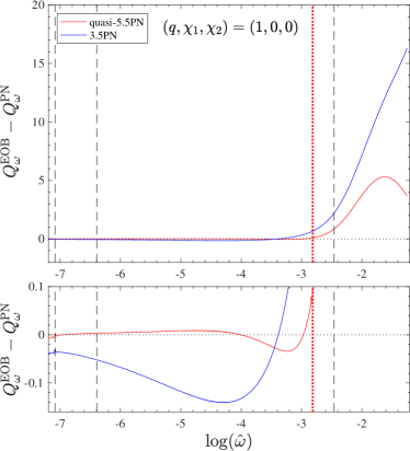
Figure 1: Comparison between the point-mass (nonspinning) orbital phasing for $q=1$ $Q_{\omega}^{\rm EOB}-Q_{\omega}^{\rm PN}$ difference up to (approximate) merger time. The vertical lines mark the 10Hz, 20Hz, 718Hz or 1024Hz for a $(1.35+1.35)M_{\odot}$ binary. The quasi-5.5PN curve is always much closer to the EOB one than the standard 3.5PN approximant.

Let us now study the performance of TaylorF2 at 5.5PN versus the full EOB phasing. We do so by comparing the corresponding $Q_{\omega}$ functions and taking the differences, similarly to what was done in Ref. Dietrich et al. (2019) for isolating the tidal part of the EOB phasing and in Ref. Nagar et al. (2019) for isolating the quadratic-in-spin part. Since we have in mind an application to a paradigmatic BNS system, Fig. 1 only focuses on the $q=1$ case. We show our results in terms of differences between the EOB and the PN curves, $Q_{\omega}^{\rm EOB}-Q_{\omega}^{\rm PN}$. The top panel of the figure illustrates the full phasing acceleration evolution, up to the peak of the EOB orbital frequency that is identified with the merger. The bottom panel is a close up on the inspiral part. The vertical lines corresponds (from left to right) to 10Hz, 20Hz, 718Hz and 1024Hz for a fiducial equal-mass BNS system with $(1.35+1.35)M_{\odot}$. The 718Hz line corresponds to $\hat{\omega}=0.06$, that roughly corresponds to the NR contact frequency Bernuzzi et al. (2012). The figure highlights that the quasi-5.5PN approximant delivers a rather good representation of the point-mass EOB phasing precisely up to $\hat{\omega}=0.06$. Table 1 reports the phase difference

$$\Delta\phi_{(\hat{\omega}_{0},\hat{\omega}_{1})}=\int_{\hat{\omega}_{0}}^{\hat{\omega}_{1}}\Delta Q_{\omega}d\log\hat{\omega}\ ,$$ (8)

accumulated between the frequencies $[\hat{\omega}_{0},\hat{\omega}_{1}]$ (or equivalently $[f_{0},f_{1}]$ in physical units) marked by vertical lines in the plots. The numbers in the table illustrate quantitatively how the 5.5PN phasing approximant delivers a phasing description that is, by itself, more EOB compatible than the standarly used 3.5PN one. Note that this is achieved even if the EOB incorporates the effective, NR-informed, $a_{c}^{6}(\nu)$ parameter, that is not included in the TaylorF2 approximant.

Table 1: EOB/PN phase difference accumulated between $[f_{0},f_{1}]$. It is obtained by integrating the $\Delta Q_{\omega}^{\rm EOBPN}$’s in Fig. 1 between the corresponding values of $\log(\hat{\omega})$. The limits of integration are denoted in Hz as we want to ideally refer to the fiducial $(1.35+1.35)M_{\odot}$ binary system.

$\hat{\omega}_{0}\times 10^{4}$	$\hat{\omega}_{1}$	$f_{0}$[Hz]	$f_{1}$[Hz]	$\Delta\phi^{\rm EOBPN}_{\rm 3.5PN}$	$\Delta\phi^{\rm EOBPN}_{\rm 5.5PN}$
8.35	0.086	10	1024	0.2718	0.1364
8.35	0.060	10	718	​​​​$-0.1916$	$1.45\times 10^{-3}$
16.7	0.086	20	1024	0.3009	0.1354
16.7	0.060	20	718	​​​​$-0.1625$	$4.54\times 10^{-4}$
20.0	0.086	24	1024	0.3110	0.1348

III Application to $\tilde{\Lambda}$ inference

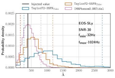
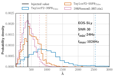
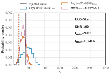
Figure 2: $1.35M_{\odot}+1.35M_{\odot}$ binary with Sly EOS. Inference of $\tilde{\Lambda}$ with different waveform model on different frequency intervals $[f_{\rm min},f_{\rm max}]$ with different SNR. The vertical line corresponds to the injected value $\tilde{\Lambda}^{\rm SLy}=392.231$. Irrespectively of the value of SNR, the 3.5PN baseline introduces a strong bias (and spread) in the measure of $\tilde{\Lambda}$. By contrast this is practically reabsorbed when using the quasi-5.5PN point-mass baseline. The dashed vertical lines corresponds to $90\%$ confidence level.

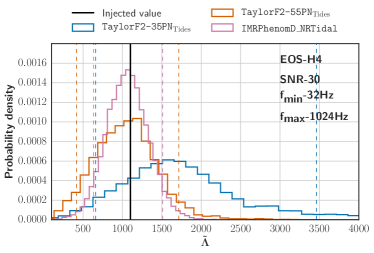
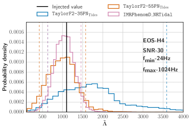
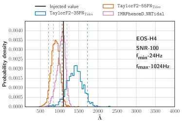
Figure 3: $1.35M_{\odot}+1.35M_{\odot}$ binary with Sly EOS. Inference of $\tilde{\Lambda}$ with different waveform model on different frequency intervals $[f_{\rm min},f_{\rm max}]$ with different SNR. The vertical line corresponds to the injected value $\tilde{\Lambda}^{\rm SLy}=1020.5$. Irrespectively of the value of SNR, the 3.5PN baseline introduces a strong bias (and spread) in the measure of $\tilde{\Lambda}$. By contrast this is practically reabsorbed when using the quasi-5.5PN point-mass baseline. The dashed vertical lines corresponds to $90\%$ confidence level.

We focus now on a BNS system to study the implication of changing the PN-accuracy of the point-mass baseline on the estimate of the tidal polarizability parameter

$$\tilde{\Lambda}=\dfrac{16}{13}\dfrac{(m_{1}+12m_{2})m_{1}^{4}\Lambda_{1}+(m_{2}+12m_{1})m_{2}^{4}\Lambda_{2}}{M^{5}},$$ (9)

where $\Lambda^{i}\equiv 2/3k^{i}_{2}\left[c^{2}/(G{{\cal C}_{i})}\right]^{5}$ where ${\cal C}_{i}\equiv m_{i}/R_{i}$ is the compactness of each star and $k_{2}^{i}$ the corresponding quadrupolar Love number Damour (1983); Hinderer (2008); Binnington and Poisson (2009); Damour and Nagar (2009).

We construct equal-mass EOBNR hybrid BNS waveforms by matching the TEOBResumS EOB tidal model Nagar et al. (2018) to state-of-the-art NR simulations of the CoRe collaboration Dietrich et al. (2019). Note that the version of TEOBResumS used here does not incorporate the analytical developments of Refs. Nagar et al. (2019); Akcay et al. (2019). Two fiducial waveforms are considered here corresponding to two nonspinning, equal-mass ($1.35M_{\odot}+1.35M_{\odot}$) BNS models described by the SLy and H4 EOS. The corresponding values of the tidal parameters are $\tilde{\Lambda}=392.231$ (Sly EOS) and $\tilde{\Lambda}=1110.5$ (H4 EOS) [For equal masses $\tilde{\Lambda}=\Lambda_{1}=\Lambda_{2}$.] The waveforms are injected at SNR of 30 and 100 into a fiducial data stream of the LIGO detectors Aasi et al. (2015). We assume the projected noise curve for the Advanced LIGO detectors in the zero-detuned high-power configuration (ZDHP) Shoemaker and no actual noise is added to the data.

Table 2: Data behind Figs. 2 and 3. For each measured quantity, chirp mass ${\cal M}$, symmetric mass ratio $\nu$ and tidal polarizability $\tilde{\Lambda}$, the colums report: the injected value; the minimum value of frequency considered, either 24Hz or 32Hz; the combination EOS-SNR; finally, the last three columns list the median values measured with the three different waveform approximants with the $90\%$ credible interval. The last row of the table shows the average waveform generation time for each approximant, assuming starting frequency of 24Hz.

	Injected Value	$f_{\rm min}$	EOS	SNR	TaylorF2 3.5PN	TaylorF2 5.5PN	IMRPhenomD_NRTidal
$\mathcal{M}$	1.1752	$24$ Hz	SLy	30	$1.1753^{1.1755}_{1.1752}$	$1.1753^{1.1755}_{1.1752}$	$1.1753^{1.1755}_{1.1752}$
			H4	30	$1.1753^{1.1755}_{1.1752}$	$1.1753^{1.1755}_{1.1752}$	$1.1753^{1.1755}_{1.1752}$
			SLy	100	$1.1753^{1.1754}_{1.1752}$	$1.1753^{1.1754}_{1.1752}$	$1.1753^{1.1754}_{1.1752}$
			H4	100	$1.1753^{1.1754}_{1.1752}$	$1.1753^{1.1754}_{1.1752}$	$1.1753^{1.1754}_{1.1753}$
		$32$ Hz	SLy	30	$1.1754^{1.1757}_{1.1752}$	$1.1754^{1.1757}_{1.1752}$	$1.1754^{1.1756}_{1.1752}$
			H4	30	$1.1754^{1.1756}_{1.1751}$	$1.1754^{1.1757}_{1.1752}$	$1.1753^{1.1756}_{1.1751}$
$\nu$	0.25	$24$ Hz	SLy	30	$0.24649^{0.24996}_{0.23147}$	$0.24558^{0.24995}_{0.23135}$	$0.24636^{0.24997}_{0.23105}$
			H4	30	$0.24729^{0.24997}_{0.2338}$	$0.24581^{0.24995}_{0.23162}$	$0.2459^{0.24996}_{0.23079}$
			SLy	100	$0.24857^{0.24998}_{0.23744}$	$0.24738^{0.24995}_{0.23691}$	$0.24703^{0.24998}_{0.23292}$
			H4	100	$0.24877^{0.24997}_{0.24083}$	$0.24735^{0.24995}_{0.23694}$	$0.24702^{0.24997}_{0.23307}$
		$32$ Hz	SLy	30	$0.24658^{0.24996}_{0.23107}$	$0.2467^{0.24997}_{0.23247}$	$0.24592^{0.24997}_{0.23054}$
			H4	30	$0.24684^{0.24997}_{0.23282}$	$0.24602^{0.24995}_{0.23194}$	$0.24576^{0.24996}_{0.23051}$
$\tilde{\Lambda}$	$392$	$24$ Hz	SLy	30	$935.91^{2547.71}_{245.40}$	$517.88^{971.32}_{162.29}$	$400.47^{761.30}_{135.47}$
	$1110$		H4	30	$1690.56^{3589.6}_{632.12}$	$987.29^{1575.33}_{422.78}$	$1044.27^{1459.18}_{630.88}$
	$392$		SLy	100	$452.24^{694.52}_{180.44}$	$301.87^{459.52}_{149.57}$	$295.21^{410.31}_{162.62}$
	$1110$		H4	100	$1405.42^{1726.90}_{1065.20}$	$894.93^{1069.01}_{711.92}$	$1051.61^{1195.12}_{837.18}$
	$392$	$32$ Hz	SLy	30	$1007.47^{2743.87}_{267.25}$	$572.29^{1177.84}_{156.79}$	$419.89^{803.14}_{144.15}$
	$1110$		H4	30	$1675.67^{3464.08}_{660.31}$	$1042.61^{1713.99}_{416.23}$	$1060.44^{1509.45}_{633.25}$
Average Time					22.9 ms	32.68 ms	60.13 ms

The injected waveform is recovered with three approximants: (i) IMRPhenomD_NRTidal Dietrich et al. (2019), where the point-mass orbital phasing is obtained by a suitable representation of hybridized EOB/NR BBH waveforms, the PhenomD approximant Khan et al. (2016); (ii) TaylorF2 where the 3.5PN orbital phase is augmented by the 6PN (next-to-leading) tidal phase Vines and Flanagan (2010); (iii) the same as above where the 3.5PN orbital, nonspinning, phase is replaced by the quasi-5.5PN one. The models are implemented in the ${\tt LSC~{}Algorithm~{}Library~{}Suite~{}(LALSuite)}$. The LIGO-Virgo parameter-estimation algorithm LALInference Veitch et al. (2015)) is then employed to extract the binary properties from the signal. We use a uniform prior distribution in the interval $[1M_{\odot},3M_{\odot}]$ for the component masses, and a uniform prior between $-1$ and $1$ for both dimensionless aligned spins. We also pick a uniform prior distribution for the individual tidal parameters $\Lambda_{1,2}$ between $0$ and $5000$.

The outcome of the analysis is illustrated in Fig. 2 for the SLy EOS and and Fig. 3 the H4 EOS. We compare the inference of the tidal parameter done on two frequency intervals, $[24,1024]$ Hz and $[32,1024]$. Note that we do not extend the analysis interval even further because we know that the orbital part of the TaylorF2 approximants becomes largely inaccurate at higher frequencies. For ${\rm SNR}=30$ one finds that the 3.5PN orbital baseline induces a clear bias in $\tilde{\Lambda}$, while the quasi-5.5PN one agrees much better with the PhenomD model as well as the expected value (vertical line in the plots). Incrementing the SNR to 100, the statement only holds for the softer EOS, since for the H4 case also the 5.5PN approximant is biased, although still less than the 3.5PN one. The two figures are complemented by Table 2, that, for each choice of configuration and SNR, lists the recovered values with their 90% credible interval. The last row of the table also reports the time needed to generate a single waveform during the PE process: interestingly, the timing of the quasi-5.5PN TaylorF2 is comparable to the one of the 3.5PN approximant, i.e. it remains approximately two times faster than PhenomD_NRTidal being consistent with this latter at SNR $\lesssim 30$. This suggests that, for events similar to GW170817 or quieter, the quasi-5.5PN TaylorF2 can effectively be used in place of PhenomD_NRTidal to get an even faster, yet accurate, estimate of the parameters.

III.1 Understanding waveform systematics of the injections via the $Q_{\omega}$ analysis

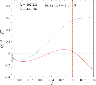
Figure 4: Heuristic explanation of the bias on $\tilde{\Lambda}$: $1.35M_{\odot}+1.35M_{\odot}$ binary, Sly EOS, $\tilde{\Lambda}=392.231$. Shown is the gauge-invariant difference $\Delta Q_{\omega}^{\rm EOBPN}\equiv Q_{\omega}^{\rm EOB}-Q_{\omega}^{\rm PN}$ between the EOB $Q_{\omega}$ and the PN $Q_{\omega}$ with the 3.5PN orbital baseline augmented by the 6PN-accurate tidal phase. Increasing the value of the tidal parameter to $\tilde{\Lambda}=442.987$ is very effective in reducing the phase difference accumulated between in the interval $\omega\in[0.02,0.06]$ (dotted vertical line) to a negligible value. Such $\hat{\omega}$ interval correponds to $f\in[24,718]$ Hz for this binary. The upper frequency limit corresponds to 957.4 Hz.

Let us finally heuristically explain why the effect of the 3.5PN-accurate orbital baseline is to bias the value of $\tilde{\Lambda}$ towards values that are larger than the theoretical expectation. Inspecting Fig. 1 one sees that the $Q_{\omega}^{\rm EOB}-Q_{\omega}^{\rm 3.5PN}$ is negative. This means that the PN phase accelerates less than the EOB one, namely the inspiral occurs more slowly in the 3.5PN phasing description than in the EOB one. Loosely speaking, one may think that the gravitational interaction behind the 3.5PN-accurate orbital phasing is less attractive than what predicted by the EOB model. Evidently, this effect might be compensated by and additional part in the total PN phasing that stems for a part of the dynamics that is intrinsically attractive and that could compensate for the inaccurate behavior of the 3.5 PN. Since eventually the phase difference is given by an integral, two effects of opposite sign can mutually compensate and thus generate a PN-based frequency phase that is compatible with the EOB one. Since tidal interactions are attractive, the corresponding part of the phasing is naturally able to compensate the repulsive character of the orbital phasing. For this compensation to be effective, it may happen that $\tilde{\Lambda}$ has to be larger than the theoretically correct one that accounts for the tidal interaction (at leading order) in the EOB waveform.

Such intuitive explanation is put on more solid ground in Fig. 4. The figure refers to the SLy model and compares two EOB-PN $Q_{\omega}$ differences $\Delta Q_{\omega}^{\rm EOBPN}\equiv Q_{\omega}^{\rm EOB}-Q_{\omega}^{\rm PN}$, where the $Q_{\omega}^{\rm EOB}$ is the complete function, while $Q_{\omega}^{\rm PN}$ is obtained summing together the 3.5PN orbital phase and the 6PN-accurate tidal phase Vines et al. (2011). When we use the theoretically correct value of $\tilde{\Lambda}=\Lambda_{1}=\Lambda_{2}=392.231$ the phase difference in the interval $\hat{\omega}\in[\hat{\omega}_{0},\hat{\omega}_{1}]=[0.002,0.06]$, corresponding to $f\in[20,718]$ Hz (dotted vertical line in the figure) for this binary, is $\Delta\phi_{(\hat{\omega}_{0},\hat{\omega}_{1})}\simeq-0.276$ rad. By contrast, if the value of $\tilde{\Lambda}$ is progressively increased, the accumulated phase difference between $[\hat{\omega}_{0},\hat{\omega}_{1}]$ gets reduced up to $\Delta\phi_{(\hat{\omega}_{0},\hat{\omega}_{1})}\simeq 2.429\times 10^{-4}$ for $\tilde{\Lambda}=442.987$. Note however that such analytically predicted “bias”in $\tilde{\Lambda}$ depends on the frequency interval considered: if we extended the integration up to $\hat{\omega}_{1}\simeq 0.08$ (corresponding to 957.4 Hz) one finds that a similarly small accumulated phase difference $\Delta\phi_{0.002,0.08}\simeq 5.0\times 10^{-5}$ is obtained for $\tilde{\Lambda}=424.08$, i.e. the analytical bias is reduced. This fact looks counterintuitive: a result obtained with a PN approximant is not, a priori, expected to improve when including higher frequencies. By contrast, the fact that the analytic bias is (slightly) reduced increasing $\hat{\omega}_{1}$ just illustrates the lack of robustness as well as the lack of predictive power of the approximant in the strong-field regime. Generally speaking, one sees that the combination of 3.5PN orbital phase with 6PN tidal phase may result in a waveform that is effectual with respect the EOB one, in the sense that the noise-weighted scalar product will be of order unity, but with an incorrect value of the tidal parameter. This simple example is helpful to intuitively understand how the incorrect behavior of the point-mass nonspinning phasing can eventually result in a bias towards larger values of $\tilde{\Lambda}$. Interestingly, this value is close to the value obtained with SNR=100 (see left-bottom panel of Fig. 2). Although the analysis of Fig. 4 certainly cannot replace an injection-recovery study, it should be kept in mind as a complementary tool to interpret its outcome within a simple, intuitive but quantitative, framework.

IV Conclusions

Our results can be summarized as follows:

1. Starting from the EOB resummed expressions for the energy flux and energy along circular orbits, we have computed a TaylorF2 point-mass, nonspinning, approximant at formal 5.5PN order. Such quasi-5.5PN approximant depends on some, yet uncalculated, $\nu$-dependent, PN parameters that are set to zero.

2. Among various truncations of the 5.5PN approximant (3.5PN, 4PN, 4.5PN, 5PN, see Appendix A, we have found that the 5.5PN phasing performs best when compared with the complete point-mass phasing obtained with ${\tt TEOBResumS}$. Such phasing comparison was done exploiting its gauge-invariant description through the $Q_{\omega}=\hat{\omega}^{2}/\dot{\hat{\omega}}$ function. The main outcome of this analysis is that the EOB-derived quasi-5.5PN approximant is remakably close to the complete EOB phasing up to the late inspiral (e.g. $\hat{\omega}\simeq 0.06$) and performs better than the standard (analytically complete) 3.5PN one. We tested that the performaces remain robust for unequal masses up to $q=2$ and aligned spin cases with dimensionless spin magnitudes up to $\chi\sim\pm 0.1$.

3. To assess the use of the 5.5PN approximant in GW parameter estimations, we considered injection studies with hybrid waveforms of GW170817-like sources. The improved TaylorF2 point-mass baseline reduces (or even eliminates) the biases on the measurability of the tidal polarizability parameter $\tilde{\Lambda}$ instead produced by the use the standard 3.5PN point-mass baseline. Therefore, the new 5.5PN approximant can be faithfully and effectively used in matched filtered searches and Bayesian parameter estimation.

We recommend to use the new quasi-5.5PN approximant to improve the performance of the TaylorF2 and substitute it to the 3.5PN in searches/parameter estimation. To ease this task, we have implemented all the new PN terms up to 5.5PN in the ${\tt LSC~{}Algorithm~{}Library~{}Suite~{}(LALSuite)}$.

The performances of the 5.5PN approximant could be further improved towards higher frequencies by carefully tuning some of the free parameters. A preliminary investigation based on a equal masses nonspinning BNS is presented at the end of Appendix A). We find that by tuning the 5PN parameter $a_{6}^{c}$ and the 4PN coefficient $c^{\rm 4PN}_{22}$ entering the $\ell=m=2$ waveform amplitude, the phase difference between such flexed PN approximant and the EOB phasing is negligible essentially up to merger. This indicates that, while the PN series keeps oscillating even when high order terms come into play, future work might be devoted to effectively minimize such oscillations by suitably tuning such parameters.

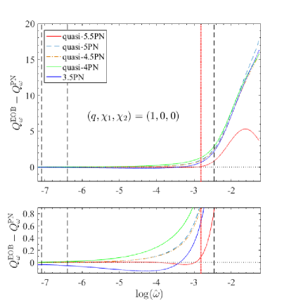
Figure 5: Comparison between the point-mass (nonspinning) orbital phasing for $q=1$ $Q_{\omega}^{\rm EOB}-Q_{\omega}^{\rm PN}$ difference up to (approximate) merger time. The vertical lines mark the 10Hz, 20Hz, 718Hz or 1024Hz for a $(1.35+1.35)M_{\odot}$ binary. The quasi-5.5PN curve is always much closer to the EOB one than the other PN order approximants. See Table 3 for the accumulated phase differences.

Table 3: EOB/PN phase difference accumulated between $[f_{0},f_{1}]$. It is obtained by integrating the $\Delta Q_{\omega}^{\rm EOBPN}$’s in Fig. 5 between the corresponding values of $\log(\hat{\omega})$, also listed in the table. The limits of integration denoted in Hz refer to the fiducial $(1.35+1.35)M_{\odot}$ binary system.

$\hat{\omega}_{0}$ $\times 10^{4}$	$\hat{\omega}_{1}$	$f_{0}$[Hz]	$f_{1}$[Hz]	$\Delta\phi^{\rm EOBPN}_{\rm 5PN}$	$\Delta\phi^{\rm EOBPN}_{\rm 4.5PN}$	$\Delta\phi^{\rm EOBPN}_{\rm 4PN}$
$8.35$	0.086	10	1024	1.0805	1.0109	1.6306
$8.35$	0.060	10	718	0.4984	0.469	0.9241
$16.7$	0.086	20	1024	1.079	1.0094	1.6235
$16.7$	0.060	20	718	0.4970	0.4675	0.9170
$20.0$	0.086	24	1024	1.0781	1.0085	1.6203

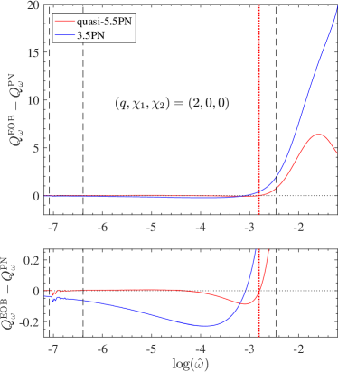
Figure 6: Robustness of the quasi-5.5PN TaylorF2 approximant versus mass ratio. The vertical lines correspond to the same four values of $[\hat{\omega}_{1},\hat{\omega}_{2}]$ listed in the first two columns of Table 3.

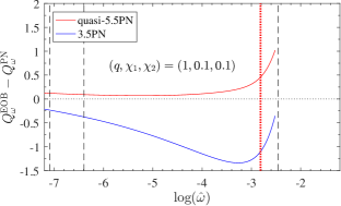
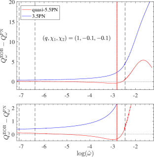
Figure 7: Robustness of the quasi-5.5PN TaylorF2 approximant versus spin: spins aligned (top) and spins anti-aligned (bottom) with the orbital angular momentum. The EOB/PN agreement is always improved by the use of the quasi-5.5PN orbital phasing. The vertical lines correspond to the same four values of $[\hat{\omega}_{1},\hat{\omega}_{2}]$ listed in the first two columns of Table 3.

Appendix A Why quasi-5.5PN?

Post-Newtonian expansion are truncated asymptotic series, so it is not a priori granted that by increasing the PN order one will automatically get a better approximation to the exact result. The choice of using the quasi-5.5PN ${\tt TaylorF2}$ for the injection study of Sec. III was made after having carefully analyzed all the previous quasi-PN orders beyond 3.5PN and having compared each PN-truncation of the $Q_{\omega}$ function to the corresponding outcome of TEOBResumS. The result of this analysis is shown in Fig. 5, that illustrates how the quasi-5.5PN $Q_{\omega}^{\rm EOB}-Q_{\omega}^{\rm PN}$ difference remains consistently close to zero for a frequency interval that is much longer than for any other lower-PN truncation. This finding justifies our choice of focalizing specifically on the quasi-5.5PN approximant in the main text.

With this PN order, the first natural question that follows is whether there is some simple way to improve the accuracy of the approximant just by tuning some of its (many) free parameters. Before entering this discussion, the simplest thing to do is to incorporate more analytical information ,e.g. instead of using $a_{6}^{c}=0$ incorporating either the analytical gravitational self-force value $a_{6}^{c}(0)$, that was obtained in Refs. Barausse et al. (2012); Bini and Damour (2014)

$$a_{6}^{c}(0) =-\frac{1066621}{1575}-\frac{14008\gamma}{105}+\frac{246367\pi^{2}}{3072}$$

$$-\frac{31736\log(2)}{105}+\frac{243\log(3)}{7},$$ (10)

or even the numerical-relativity informed one Nagar et al. (2016)

$$a_{6,\rm NR}^{c}(\nu)=3097.3\nu^{2}-1330.6\nu+81.38.$$ (11)

Although these two functions encode physically correct effect (though only effectively for $a_{6,\rm NR}^{c}(\nu)$) they turn out, both, to increase the repulsive character of the approximant, without any real advantage. In practice, when the values above are used, one get an acceptable EOB/PN agreement only up to $\hat{\omega}\approx 0.02$.

From the PN point of view, we expect from Table II of Messina et al. (2018) that the order of magnitude of the various $c_{\ell m}^{\rm PN}$ coefficient is small. This is the rational behind our conservative choice of simply setting then to zero. Still, one could think to use some of these coefficients, as well as $a_{6}^{c}$ as tunable parameter and investigate whether it is possible to flex the quasi-5.5PN TaylorF2 approximant so as to reduce the EOB/PN disagreement even to frequencies higher than $0.06$.

As a proof of principle, we explored that this is the case considering the $q=1$ case and flexing, at the same time, both $a_{6}^{c}$ and $c_{22}^{\rm 4PN}$, that are, in sense, the lowest-order unknown coefficients in the model. One easily finds that fixing $a_{6}^{c}=49$ and $c_{22}^{\rm 4PN}=10.45$ the integrated EOB/PN phase difference in the point-mass sector accumulated on the interval $[\hat{\omega}_{0},\hat{\omega}_{1}]=[0.002,0.08]$ can be reduced from $0.085$ rad to $\simeq 10^{-4}$ rad.

Appendix B Mass ratio and spin

Increasing the mass ratio or the spins (to mild values) of the binary does not affect the robustness of the quasi-5.5PN, untuned, approximant. In Fig. 6 we see that the difference between the “exact” numerical $Q_{\omega}$ and the analytical one is still approximately flat for a qualitatively wide range of frequencies. Beyond that, for what concerns the spin, we show in Figs. 7 a qualitative point-mass BNS case with realistic positive and negative spins. In this case we put to zero the quadrupole-monopole interaction terms, $C_{Q1}=C_{Q2}=0$, removing the quadratic-in-spin PN corrections both in the numerical ${\tt TEOBResumS}$ model and in the analytical approximant. So contribution of the mixed $\chi_{1}\chi_{2}$ terms and the spin-orbit interaction is tested, including for completeness also the new 4PN spin-orbit Taylor-F2 term computed in Ref. Nagar et al. (2019), i.e. the $Q_{\omega}$ analogue of Eq. (48) there. While the spin-orbit terms are already contained in ${\tt TEOBResumS}$ in a resummed form, we neglect the spin cube and spin quartic PN corrections (see Nagar et al. (2019)) for simplicity, since their effect does not affect our preliminary robustness test.

Appendix C Quasi-5.5PN phasing coefficients

We report in this appendix the explicit expressions for the coefficients entering Eq. (II). For simplicity, we put to zero all the $c_{\ell m}^{\rm PN}$’s except $c_{22}^{\rm 4PN}$ and $c_{21}^{\rm 3PN}$. We have:

$$b_{2} =\frac{11\nu}{4}+\frac{743}{336}$$

$$b_{3} =-4\pi$$ (12)

$$b_{4} =\frac{617\nu^{2}}{144}+\frac{5429\nu}{1008}+\frac{3058673}{1016064}$$ (13)

$$b_{5} =\pi\left(\frac{13\nu}{8}-\frac{7729}{672}\right)$$ (14)

$$b_{6} =\frac{25565\nu^{3}}{5184}-\frac{15211\nu^{2}}{6912}+\left(-\frac{451\pi^{2}}{48}+\frac{3147553127}{12192768}\right)\nu$$

$$+\frac{856\log(x)}{105}+\frac{3424\log(2)}{105}+\frac{32\pi^{2}}{3}+\frac{1712\gamma}{105}-\frac{10817850546611}{93884313600}$$ (15)

$$b_{7} =\pi\left(\frac{14809\nu^{2}}{3024}-\frac{75703\nu}{6048}-\frac{15419335}{1016064}\right)$$ (16)

$$b_{8} =c_{21}^{\rm 3PN}\biggl{(}\frac{4}{9}\nu^{2}-\frac{1}{9}\nu\biggr{)}+\frac{73893895655\nu^{4}}{14239120896}-\frac{102008296205\nu^{3}}{11650189824}+\biggl{(}\frac{79909\pi^{2}}{24192}-\frac{300600673165997}{2563041761280}\biggr{)}\nu^{2}$$

$$+\biggl{(}-4c_{22}^{\rm 4PN}+\frac{332683\log(x)}{2205}-\frac{1860443\pi^{2}}{48384}+\frac{6252765829282087}{5695648358400}\biggr{)}\nu$$

$$+\gamma\biggl{(}\frac{665366\nu}{2205}+\frac{9203}{210}\biggr{)}+\frac{9203\log(x)}{420}+\biggl{(}\frac{47385}{1568}-\frac{47385\nu}{392}\biggr{)}\log(3)$$

$$+\biggl{(}\frac{177586\nu}{245}+\frac{50551}{882}\biggr{)}\log(2)+\frac{9049\pi^{2}}{252}-\frac{2496799162103891233}{3690780136243200}\,$$ (17)

$$b_{9} =\pi\bigg{[}\frac{2064751\nu^{3}}{399168}+\frac{9058667\nu^{2}}{254016}+\biggl{(}\frac{451\pi^{2}}{12}-\frac{298583452147}{268240896}\biggr{)}\nu$$

$$-\frac{3424}{105}\log(x)-\frac{13696}{105}\log(2)-\frac{64\pi^{2}}{3}-\frac{6848\gamma}{105}+\frac{90036665674763}{187768627200}\bigg{]}\,,$$ (18)

$$b_{10} =\frac{1}{-1+3\nu}\bigg{[}c_{21}^{\rm 3PN}\biggl{(}\frac{121}{189}\nu-\frac{2815}{756}\nu^{2}+\frac{599}{252}\nu^{3}+\frac{191}{21}\nu^{4}\biggr{)}+\biggl{(}-12c_{22}^{\rm 5PN}+54a_{6}^{c}+\frac{349c_{22}^{\rm 4PN}}{42}$$

$$-\frac{415795517\pi^{2}}{3612672}+\frac{99239192119\gamma}{18336780}+\frac{3592581310185992768897549}{292602096577251901440}+\frac{58330935\log(3)}{21952}$$

$$+\frac{117340379713\log(2)}{18336780}\biggr{)}\nu^{2}+\biggl{(}-18a_{6}^{c}+\frac{311c_{22}^{\rm 4PN}}{42}+4c_{22}^{\rm 5PN}+\frac{5451429547\pi^{2}}{32514048}$$

$$-\frac{63787407527\gamma}{36673560}-\frac{2749231177355819921781277}{216742293760927334400}-\frac{8924175\log(3)}{12544}-\frac{159943397077\log(2)}{73347120}\biggr{)}\nu$$

$$+\biggl{(}-\frac{641c_{22}^{\rm 4PN}}{7}+\frac{460519\pi^{2}}{6144}+\frac{3073896571\gamma}{3056130}+\frac{655042586669421296014259}{137157232770586828800}$$

$$-\frac{1279395\log(3)}{392}+\frac{10777949417\log(2)}{1528065}\biggr{)}\nu^{3}-\frac{2425066585102052979797\nu^{6}}{3428930819264670720}+\frac{12721434740371951621\nu^{5}}{2705270863325184}$$

$$+\left(\frac{9434797\pi^{2}}{75264}-\frac{11160810800663155149913}{1088549466433228800}\right)\nu^{4}-\frac{578223115\pi^{2}}{12192768}-\frac{6470582647\gamma}{110020680}$$

$$+\frac{1412206995432957982751}{505226791983513600}+\frac{5512455\log(3)}{87808}-\frac{53992839431\log(2)}{220041360}\bigg{]}$$

$$+\left(-\frac{6431890181\nu^{2}}{18336780}-\frac{2968141499\nu}{12224520}+\frac{6470582647}{220041360}\right)\log(x)\,,$$ (19)

$$b_{11} =\pi\bigg{[}c_{21}^{\rm 3PN}\biggl{(}-\frac{8}{3}\nu^{2}+\frac{2}{3}\nu\biggr{)}+\frac{131525414689\nu^{4}}{64076044032}-\frac{216119565695\nu^{3}}{11650189824}+\biggl{(}-\frac{2129581\pi^{2}}{16128}+\frac{5120314955146397}{1398022778880}\biggr{)}\nu^{2}$$

$$+\biggl{(}-\frac{673331\log(x)}{1260}+\frac{9003157\pi^{2}}{64512}+16c_{22}^{\rm 4PN}-\frac{471473599592788087}{76891252838400}\biggr{)}\nu$$

$$+\gamma\biggl{(}-\frac{673331\nu}{630}-\frac{3558011}{17640}\biggr{)}-\frac{3558011\log(x)}{35280}+\biggl{(}\frac{47385\nu}{196}-\frac{47385}{784}\biggr{)}\log(3)$$

$$+\biggl{(}-\frac{10504813\nu}{4410}-\frac{862549}{2520}\biggr{)}\log(2)-\frac{9439\pi^{2}}{126}+\frac{1795505143426433771}{615130022707200}\bigg{]}\ .$$ (20)

The GW phase in the SPA is computed from the $Q_{\omega}$ using (2) and it is given by the Taylor series

$$\Psi(f) =\frac{3(\pi Mf)^{-5/3}}{128\nu}\sum_{i}\varphi_{i}(\pi Mf)^{i}\ ;$$ (21)

with the coefficients:

$$\varphi_{0} =1$$ (22)

$$\varphi_{1} =0$$

$$\varphi_{2} =\frac{3715}{756}+\frac{55}{9}\nu$$

$$\varphi_{3} =-16\pi$$

$$\varphi_{4} =\frac{3085\nu^{2}}{72}+\frac{27145\nu}{504}+\frac{15293365}{508032}$$

$$\varphi_{5} =\pi\left(\frac{38645}{756}-\frac{65\nu}{9}\right)[1+\log(\pi fM)]$$

$$\varphi_{6} =-\frac{6848}{63}\log(\pi fM)-\frac{127825\nu^{3}}{1296}+\frac{76055\nu^{2}}{1728}+\biggl{(}\frac{2255\pi^{2}}{12}-\frac{15737765635}{3048192}\biggr{)}\nu-\frac{640\pi^{2}}{3}-\frac{6848\gamma}{21}$$

$$+\frac{11583231236531}{4694215680}-\frac{13696\log(2)}{21}$$

$$\varphi_{7} =\pi\biggl{(}-\frac{74045\nu^{2}}{756}+\frac{378515\nu}{1512}+\frac{77096675}{254016}\biggr{)}$$

$$\varphi_{8} =[1-\log(\pi fM)]\biggl{[}c_{21}^{\rm 3PN}\biggl{(}\frac{40\nu}{81}-\frac{160\nu^{2}}{81}\biggr{)}+\frac{160c_{22}^{\rm 4PN}\nu}{9}-\frac{369469478275\nu^{4}}{16019011008}+\frac{510041481025\nu^{3}}{13106463552}$$

$$+\biggl{(}\frac{300600673165997}{576684396288}-\frac{399545\pi^{2}}{27216}\biggr{)}\nu^{2}+\biggl{(}-\frac{5679872289503527}{1281520880640}-\frac{5322928\gamma}{3969}+\frac{9302215\pi^{2}}{54432}$$

$$-\frac{1420688\log(2)}{441}+\frac{26325\log(3)}{49}\biggr{)}\nu-\frac{90490\pi^{2}}{567}-\frac{36812\gamma}{189}+\frac{2550713843998885153}{830425530654720}-\frac{26325\log(3)}{196}$$

$$-\frac{1011020\log(2)}{3969}\biggr{]}+\biggl{(}\frac{2661464\nu}{11907}+\frac{18406}{567}\biggr{)}\log^{2}(\pi fM)$$

$$\varphi_{9} =\pi\biggl{[}-\frac{13696}{63}\log(\pi fM)+\frac{10323755\nu^{3}}{199584}+\frac{45293335\nu^{2}}{127008}+\biggl{(}\frac{2255}{6}\pi^{2}-\frac{1492917260735}{134120448}\biggr{)}\nu$$

$$-\frac{640}{3}\pi^{2}-\frac{13696\gamma}{21}+\frac{105344279473163}{18776862720}-\frac{27392\log(2)}{21}\biggr{]}$$

$$\varphi_{10} =\frac{1}{1-3\nu}\biggl{[}a_{6}^{c}(72\nu-216\nu^{2})+c_{21}^{\rm 3PN}\left(-\frac{764\nu^{4}}{21}-\frac{599\nu^{3}}{63}+\frac{2815\nu^{2}}{189}-\frac{484\nu}{189}\right)+c_{22}^{\rm 4PN}\left(\frac{2564\nu^{3}}{7}-\frac{698\nu^{2}}{21}-\frac{622\nu}{21}\right)$$ (23)

$$+c_{22}^{\rm 5PN}\left(48\nu^{2}-16\nu\right)+\left(\frac{12863780362\nu^{3}}{4584195}+\frac{13849493129\nu^{2}}{13752585}-\frac{24279431641\nu}{27505170}+\frac{6470582647}{82515510}\right)\log(\pi fM)$$

$$+\frac{2425066585102052979797\nu^{6}}{857232704816167680}-\frac{12721434740371951621\nu^{5}}{676317715831296}+\biggl{(}\frac{11160810800663155149913}{272137366608307200}$$

$$-\frac{9434797\pi^{2}}{18816}\biggr{)}\nu^{4}+\biggl{(}-\frac{857104076559310860540851}{34289308192646707200}-\frac{6147793142\gamma}{1528065}-\frac{460519\pi^{2}}{1536}$$

$$-\frac{43111797668\log(2)}{1528065}+\frac{1279395\log(3)}{98}\biggr{)}\nu^{3}+\biggl{(}-\frac{18736399363805057301105217}{365752620721564876800}-\frac{99239192119\gamma}{4584195}$$

$$+\frac{415795517\pi^{2}}{903168}-\frac{117340379713\log(2)}{4584195}-\frac{58330935\log(3)}{5488}\biggr{)}\nu^{2}+\biggl{(}\frac{569935181259668744781113}{10837114688046366720}$$

$$+\frac{63787407527\gamma}{9168390}-\frac{5451429547\pi^{2}}{8128512}+\frac{159943397077\log(2)}{18336780}+\frac{8924175\log(3)}{3136}\biggr{)}\nu+\frac{578223115\pi^{2}}{3048192}$$

$$+\frac{6470582647\gamma}{27505170}-\frac{1433006523295407126559}{126306697995878400}-\frac{5512455\log(3)}{21952}+\frac{53992839431\log(2)}{55010340}\biggr{]}$$

$$\varphi_{11} =\pi\biggl{[}c_{21}^{\rm 3PN}\biggl{(}-\frac{160\nu^{2}}{27}+\frac{40\nu}{27}\biggr{)}+\frac{320c_{22}^{\rm 4PN}\nu}{9}-\biggl{(}\frac{1346662\nu}{1701}+\frac{3558011}{23814}\biggr{)}\log(\pi fM)$$

$$+\frac{657627073445\nu^{4}}{144171099072}-\frac{1080597828475\nu^{3}}{26212927104}+\frac{5120314955146397\nu^{2}}{629110250496}+\pi^{2}\biggl{(}-\frac{10647905\nu^{2}}{36288}+\frac{45015785\nu}{145152}$$

$$-\frac{94390}{567}\biggr{)}+\biggl{(}-\frac{1346662\gamma}{567}-\frac{430383707398397047}{34601063777280}+\frac{26325}{49}\log(3)-\frac{21009626\log(2)}{3969}\biggr{)}\nu-\frac{3558011\gamma}{7938}$$

$$+\frac{1857541407236594411}{276808510218240}-\frac{26325\log(3)}{196}-\frac{862549\log(2)}{1134}\biggr{]}$$

References

- Abbott et al. (2017) B. P. Abbott et al. (Virgo, LIGO Scientific), Phys. Rev. Lett. 119, 161101 (2017), arXiv:1710.05832 [gr-qc] .
- Damour et al. (2012) T. Damour, A. Nagar, and L. Villain, Phys.Rev. D85, 123007 (2012), arXiv:1203.4352 [gr-qc] .
- Del Pozzo et al. (2013) W. Del Pozzo, T. G. F. Li, M. Agathos, C. Van Den Broeck, and S. Vitale, Phys. Rev. Lett. 111, 071101 (2013), arXiv:1307.8338 [gr-qc] .
- Abbott et al. (2018a) B. P. Abbott et al. (LIGO Scientific, Virgo), Phys. Rev. Lett. 121, 161101 (2018a), arXiv:1805.11581 [gr-qc] .
- Abbott et al. (2019) B. P. Abbott et al. (LIGO Scientific, Virgo), Phys. Rev. X9, 011001 (2019), arXiv:1805.11579 [gr-qc] .
- Abbott et al. (2018b) B. P. Abbott et al. (LIGO Scientific, Virgo), (2018b), arXiv:1811.12907 [astro-ph.HE] .
- Favata (2014) M. Favata, Phys.Rev.Lett. 112, 101101 (2014), arXiv:1310.8288 [gr-qc] .
- Wade et al. (2014) L. Wade, J. D. E. Creighton, E. Ochsner, B. D. Lackey, B. F. Farr, T. B. Littenberg, and V. Raymond, Phys. Rev. D89, 103012 (2014), arXiv:1402.5156 [gr-qc] .
- Dudi et al. (2018) R. Dudi, F. Pannarale, T. Dietrich, M. Hannam, S. Bernuzzi, F. Ohme, and B. Bruegmann, (2018), arXiv:1808.09749 [gr-qc] .
- Buonanno and Damour (1999) A. Buonanno and T. Damour, Phys. Rev. D59, 084006 (1999), arXiv:gr-qc/9811091 .
- Buonanno and Damour (2000) A. Buonanno and T. Damour, Phys. Rev. D62, 064015 (2000), arXiv:gr-qc/0001013 .
- Damour and Nagar (2010) T. Damour and A. Nagar, Phys. Rev. D81, 084016 (2010), arXiv:0911.5041 [gr-qc] .
- Bernuzzi et al. (2015) S. Bernuzzi, A. Nagar, T. Dietrich, and T. Damour, Phys.Rev.Lett. 114, 161103 (2015), arXiv:1412.4553 [gr-qc] .
- Hinderer et al. (2016) T. Hinderer et al., Phys. Rev. Lett. 116, 181101 (2016), arXiv:1602.00599 [gr-qc] .
- Steinhoff et al. (2016) J. Steinhoff, T. Hinderer, A. Buonanno, and A. Taracchini, Phys. Rev. D94, 104028 (2016), arXiv:1608.01907 [gr-qc] .
- Nagar et al. (2018) A. Nagar et al., Phys. Rev. D98, 104052 (2018), arXiv:1806.01772 [gr-qc] .
- Akcay et al. (2019) S. Akcay, S. Bernuzzi, F. Messina, A. Nagar, N. Ortiz, and P. Rettegno, Phys. Rev. D99, 044051 (2019), arXiv:1812.02744 [gr-qc] .
- Nagar et al. (2019) A. Nagar, F. Messina, P. Rettegno, D. Bini, T. Damour, A. Geralico, S. Akcay, and S. Bernuzzi, Phys. Rev. D99, 044007 (2019), arXiv:1812.07923 [gr-qc] .
- Lackey et al. (2017) B. D. Lackey, S. Bernuzzi, C. R. Galley, J. Meidam, and C. Van Den Broeck, Phys. Rev. D95, 104036 (2017), arXiv:1610.04742 [gr-qc] .
- Lackey et al. (2018) B. D. Lackey, M. Pürrer, A. Taracchini, and S. Marsat, (2018), arXiv:1812.08643 [gr-qc] .
- Dietrich et al. (2017) T. Dietrich, S. Bernuzzi, and W. Tichy, Phys. Rev. D96, 121501 (2017), arXiv:1706.02969 [gr-qc] .
- Dietrich et al. (2019) T. Dietrich et al., Phys. Rev. D99, 024029 (2019), arXiv:1804.02235 [gr-qc] .
- Nagar and Rettegno (2019) A. Nagar and P. Rettegno, Phys. Rev. D99, 021501 (2019), arXiv:1805.03891 [gr-qc] .
- Samajdar and Dietrich (2018) A. Samajdar and T. Dietrich, Phys. Rev. D98, 124030 (2018), arXiv:1810.03936 [gr-qc] .
- Messina and Nagar (2017) F. Messina and A. Nagar, Phys. Rev. D95, 124001 (2017), [Erratum: Phys. Rev.D96,no.4,049907(2017)], arXiv:1703.08107 [gr-qc] .
- Damour et al. (2001) T. Damour, B. R. Iyer, and B. S. Sathyaprakash, Phys. Rev. D63, 044023 (2001), [Erratum: Phys. Rev.D72,029902(2005)], arXiv:gr-qc/0010009 [gr-qc] .
- Damour et al. (2009) T. Damour, B. R. Iyer, and A. Nagar, Phys. Rev. D79, 064004 (2009), arXiv:0811.2069 [gr-qc] .
- Faye et al. (2015) G. Faye, L. Blanchet, and B. R. Iyer, Class. Quant. Grav. 32, 045016 (2015), arXiv:1409.3546 [gr-qc] .
- Messina et al. (2018) F. Messina, A. Maldarella, and A. Nagar, Phys. Rev. D97, 084016 (2018), arXiv:1801.02366 [gr-qc] .
- Bernuzzi et al. (2012) S. Bernuzzi, A. Nagar, M. Thierfelder, and B. Brügmann, Phys.Rev. D86, 044030 (2012), arXiv:1205.3403 [gr-qc] .
- Damour (1983) T. Damour, in Gravitational Radiation, edited by N. Deruelle and T. Piran (North-Holland, Amsterdam, 1983) pp. 59–144.
- Hinderer (2008) T. Hinderer, Astrophys.J. 677, 1216 (2008), arXiv:0711.2420 [astro-ph] .
- Binnington and Poisson (2009) T. Binnington and E. Poisson, Phys. Rev. D80, 084018 (2009), arXiv:0906.1366 [gr-qc] .
- Damour and Nagar (2009) T. Damour and A. Nagar, Phys. Rev. D80, 084035 (2009), arXiv:0906.0096 [gr-qc] .
- Aasi et al. (2015) J. Aasi et al. (LIGO Scientific), Class. Quant. Grav. 32, 074001 (2015), arXiv:1411.4547 [gr-qc] .
- (36) D. Shoemaker, https://dcc.ligo.org/cgi-bin/DocDB/ShowDocument?docid=2974 .
- Khan et al. (2016) S. Khan, S. Husa, M. Hannam, F. Ohme, M. Pürrer, X. Jiménez Forteza, and A. Bohé, Phys. Rev. D93, 044007 (2016), arXiv:1508.07253 [gr-qc] .
- Vines and Flanagan (2010) J. E. Vines and E. E. Flanagan, Phys. Rev. D88, 024046 (2010), arXiv:1009.4919 [gr-qc] .
- Veitch et al. (2015) J. Veitch et al., Phys. Rev. D91, 042003 (2015), arXiv:1409.7215 [gr-qc] .
- Vines et al. (2011) J. Vines, E. E. Flanagan, and T. Hinderer, Phys. Rev. D83, 084051 (2011), arXiv:1101.1673 [gr-qc] .
- Barausse et al. (2012) E. Barausse, A. Buonanno, and A. Le Tiec, Phys.Rev. D85, 064010 (2012), arXiv:1111.5610 [gr-qc] .
- Bini and Damour (2014) D. Bini and T. Damour, Phys.Rev. D89, 064063 (2014), arXiv:1312.2503 [gr-qc] .
- Nagar et al. (2016) A. Nagar, T. Damour, C. Reisswig, and D. Pollney, Phys. Rev. D93, 044046 (2016), arXiv:1506.08457 [gr-qc] .