Entropy driven transformations of statistical hypersurfaces

Abstract

Deformations of geometric characteristics of statistical hypersurfaces governed by the law of growth of entropy are studied. Both general and special cases of deformations are considered. The basic structure of the statistical hypersurface is explored through a differential relation for the variables, and connections with the replicator dynamics for Gibbs’ weights are highlighted. Ideal and super-ideal cases are analysed, also considering their integral characteristics.

Department of Mathematics and Physics “Ennio De Giorgi”,

University of Salento

and INFN, Sezione di Lecce

Lecce 73100, Italy

Keywords— Hypersurface, entropy, deformation

Mathematics Subject Classification 2000: 51P05, 82B05, 05D05

1 Introduction

Surfaces, hypersurfaces and their dynamics (deformations) are key ingredients in a broad variety of mathematical problems and phenomena in physics (see e.g. [1, 2, 3, 4, 5, 6]). In mathematics, the mechanisms governing the deformation of surfaces vary from the classical one, which preserves certain characteristics of surfaces (see e.g. [1, 2, 3]), to those described by integrable partial differential equations [7, 8, 9]. In physics, surfaces and hypersurfaces are forced to deform due to certain effects varying from a simple change of pressure inside a soap bubble to the interaction of world-sheets with background in string theory (see e.g. [4, 5, 6]).

Recently we considered [10] a special class of hypersurfaces inspired by the basic formula for the free energy in statistical physics (see e.g. [11]). This approach is aimed at identifying and, then, relating the microscopic and macroscopic sectors in statistical models. Such a purpose suggests introducing more spaces and a mapping relating them. The focus on mappings between spaces allows one to deal with families of statistical models, which is a useful approach in the analysis of complex systems.

In [10] we focused on parametric families of systems. In particular, statistical hypersurfaces have been defined by the formula

$$x_{n+1}=\ln\left(\sum_{\alpha=1}^{m}e^{f_{\alpha}(x_{1},\dots,x_{n})}\right)$$ (1.1)

where $x_{1},\dots,x_{n},x_{n+1}$ are Cartesian coordinates in $\mathbb{R}^{n+1}$ and $f_{\alpha}(x_{1},\dots,x_{n})$ are certain functions. The mapping (1.1) leads to the representation of the set of parameters as a $n$-dimensional hypersurface embedded in a $(n+1)$-dimensional ambient space. If the ambient space is endowed with a metric structure, this hypersurface inherits metric properties, which can be used to study and compare characteristic features of statistical models defined by different parameters. The role of physical interactions and phase transitions [11] can be easily discussed in this geometric framework. In particular, the notion on “ideal model” can be related to a special (translational) symmetry. On the other hand, the basic geometric characteristics of such hypersurfaces have rather special properties, which can be expressed in terms of mean values calculated with Gibbs’ distribution

$$w_{\alpha}:=\frac{e^{f_{\alpha}}}{\sum_{\beta=1}^{m}e^{f_{\beta}}},\quad\alpha=1,\dots,m.$$ (1.2)

Within such probabilistic view, the entropy defined by the standard formula [11]

$$S:=-\sum_{\alpha=1}^{m}w_{\alpha}\ln w_{\alpha}$$ (1.3)

has a simple geometrical meaning. Namely [10],

$$S=x_{n+1}-\overline{f}$$ (1.4)

where $\overline{f}$ is the mean value $\overline{f}:=\sum_{\alpha=1}^{m}w_{\alpha}f_{\alpha}$. For the super-ideal case $m=n$ and $f_{\alpha}=x_{\alpha}$, the entropy (1.4) is $S=\sqrt{\det\mathbf{g}}\vec{X}\cdot\vec{N}$, where $\vec{X}$ and $\vec{N}$ are the position vector and the normal vector at the point of the hypersurface (1.1), respectively.

The natural appearance of entropy (1.3)-(1.4) for the statistical hypersurfaces (1.1) suggests to consider the class of their deformations, transformations, and dynamics which are governed by the most fundamental property of entropy, namely, by the law of growth of entropy for isolated macroscopic systems [11].

The present paper is devoted to the analysis of geometrical characteristics of such entropy-driven transformations of statistical hypersurfaces. It is shown that the general deformations of statistical hypersurfaces corresponding to increasing entropy are characterised by the conditions

$$\overline{\delta f}>\delta\overline{f},\quad\overline{f\cdot\delta f}<\overline{f}\cdot\delta\overline{f}.$$

It is also highlighted that the variation of principal curvatures is linked to the tendency to stability or to a departure from it.

We extend the analysis in [10] discussing two classes of deformations. The first class includes deformations due to variations of variables $\boldsymbol{x}$ (parametric transformations), while the second class includes non-parametric transformations where functions $f_{\alpha}$ are changed. The case of affine functions $f_{\alpha}$ and, in particular, linear and super-ideal cases are studied in more details. It is shown that, in the linear case, the variation of the entropy between two regions of different statistical hypersurfaces is proportional to the volume of a domain in $\mathbb{R}^{n+1}$ bounded by them. A connection with replicator dynamics is also noted.

The paper is organized as follows. Some general formulas for statistical hypersurfaces are presented in Section 2. General variations of entropy and their properties are considered in Section 3. The interrelation between principal curvatures and the second law of thermodynamics is discussed in Section 4. The effects of deformations on statistical weights are investigated in Section 5 in terms of a differential characterization of the statistical mapping and a relation with the replicator dynamics. Ideal and super-ideal statistical hypersurfaces are studied in Section 6. Some possible future developments are noted in Section 7.

2 Statistical hypersurfaces and their deformations

2.1 Brief summary on statistical hypersurfaces and their tropical limit

Here, for convenience, we first reproduce some basic results of the paper [10]. In the rest of the paper, we will denote the local coordinates in $\mathbb{R}^{n}$ and in $\mathbb{R}^{m}$ as $\boldsymbol{x}$ and $\vec{f}$, respectively.

The induced metric $\mathbf{g}$ of the hypersurface $V_{n}\subseteq\mathbb{R}^{n+1}$ defined by the formula (1.1) is

$$g_{ik}=\delta_{ik}+\overline{f_{i}}\cdot\overline{f_{k}}$$ (2.1)

where

$$\overline{f_{i}}:=\sum_{\alpha=1}^{m}w_{\alpha}\frac{\partial f_{\alpha}}{\partial x_{i}},\quad i=1,\dots,n.$$ (2.2)

The position vector $\vec{X}$ for a point on $V_{n}$ and the corresponding normal vector $\vec{N}$ are

$$\vec{X}= (x_{1},\dots,x_{n},x_{n+1}),$$

$$\vec{N}= \frac{1}{\sqrt{\det\mathbf{g}}}\left(-\overline{f_{1}},\dots,-\overline{f_{n}},1\right)$$ (2.3)

where $\det\mathbf{g}=1+\sum_{i=1}^{n}\overline{f_{i}}^{2}$.

The second fundamental form $\Omega_{ik}$ is given by

$$\Omega_{ik}=\frac{1}{\sqrt{\det\mathbf{g}}}\left(\overline{f}_{(ik)}-\overline{f_{i}}\cdot\overline{f_{k}}\right)$$ (2.4)

where

$$\overline{f}_{(ik)}:=\sum_{\alpha=1}^{m}w_{\alpha}\left(\frac{\partial^{2}f_{\alpha}}{\partial x_{i}\partial x_{k}}+\frac{\partial f_{\alpha}}{\partial x_{i}}\cdot\frac{\partial f_{\alpha}}{x_{k}}\right),\quad i,k=1,\dots,n.$$ (2.5)

The Riemann curvature tensor is

$$R_{iklj}=\Omega_{il}\Omega_{kj}-\Omega_{kl}\Omega_{ij},\quad i,k,l,j=1,\dots,n.$$ (2.6)

and the Gauss-Kronecker curvature is given by

$$K=\frac{\det\left|\overline{f}_{(ik)}-\overline{f_{i}}\cdot\overline{f_{k}}\right|}{\left(1+\sum_{l=1}^{n}\overline{f_{l}}^{2}\right)^{\frac{n+2}{2}}}.$$ (2.7)

The entropy $S$ (1.4) is equivalent to [10]

$$S=\sqrt{\det\mathbf{g}}\vec{X}\cdot\vec{N}+\sum_{\alpha=1}^{m}w_{\alpha}\left(\sum_{i=1}^{n}x_{i}\frac{\partial f_{\alpha}}{\partial x_{i}}-f_{\alpha}\right)$$ (2.8)

which takes the form

$$S=\sqrt{\det\mathbf{g}}\vec{X}\cdot\vec{N}$$ (2.9)

in the super-ideal case ($f_{\alpha}=x_{\alpha}$). In all these formulae, a hypersurface associated with the physical system is specified by the choice of functions $f_{\alpha}(\boldsymbol{x})$, while $x_{1},\dots,x_{n}$ are local coordinates (parameters which characterise the state of the system).

The definition of a geometric framework to analyse statistical models also gives a natural setting to study their tropical limit, which is related to Maslov’s dequantization and ultradiscretization procedures. Tropical structures can be obtained from standard (real or complex) ones through the limit $\varepsilon\rightarrow 0^{+}$ for the following family of ring operations

$$x\oplus_{\varepsilon}y := \varepsilon\cdot\ln\left(e^{\frac{x}{\varepsilon}}+e^{\frac{x}{\varepsilon}}\right),$$

$$x\odot_{\varepsilon}y := \varepsilon\cdot\ln\left(e^{\frac{x}{\varepsilon}}\cdot e^{\frac{x}{\varepsilon}}\right)=x+y.$$ (2.10)

The exploration of the tropical limit in statistical physics naturally follows from the expression (1.1). In this case, the Boltzmann constant $k_{B}$ plays the role of the parameter $\varepsilon$ in the formal limit (2.10). A first study in this direction was carried out in [12] with $f_{\alpha}=\frac{T\cdot S_{\alpha}-E_{\alpha}}{k_{B}T}$, where $T$ is the absolute temperature, $\{E_{\alpha}\}$ is the energy spectrum of the system, and $\exp\frac{S_{\alpha}}{k_{B}}$ represents the degeneracy associated with $E_{\alpha}$. This approach offers new techniques to deal with systems with highly degenerated energy levels, e.g. frustrated systems.

The tropical limit of statistical models has been extended to more general cases in [10] to meet the formalism of statistical hypersurfaces. This extension has led to the identification of different kinds of tropical limit based on the choice of independent variables $\boldsymbol{x}$ or dependent ones $f_{\alpha}$ for the limit procedure.

An investigation of formal tropical structures in the context of statistical physics has been carried out in [13] focusing on algebraic aspects.

2.2 General deformations of statistical hypersurfaces

Now let us consider deformations of a statistical hypersurface generated by general infinitesimal variations of functions $f_{\alpha}\mapsto f_{\alpha}+\delta f_{\alpha}$, $\alpha=1,\dots,m$. Using the expressions (2.1)-(2.7), one easily gets the general variations of these quantities:

$$\delta g_{ik}=\delta\overline{f_{i}}\cdot\overline{f_{k}}+\overline{f_{i}}\cdot\delta\overline{f_{k}},$$ (2.11)

$$\delta\Omega_{ik}=-\frac{1}{2}\frac{\text{tr}(\delta\mathbf{g})}{(\det\mathbf{g})^{3/2}}\cdot\left(\overline{f}_{(ik)}-\overline{f_{i}}\cdot\overline{f_{k}}\right)+\frac{1}{(\det\mathbf{g})^{1/2}}\left(\delta\overline{f}_{(ik)}-\delta g_{ik}\right)$$ (2.12)

and

$$\delta K=\frac{\delta(\det\left|\overline{f}_{(ik)}-\overline{f_{i}}\cdot\overline{f_{k}}\right|)}{\det\mathbf{g}^{(n+2)/2}}-(n+2)\cdot\frac{\det\left|\overline{f}_{(ik)}-\overline{f_{i}}\cdot\overline{f_{k}}\right|\cdot\text{tr}(\delta\mathbf{g})}{\det\mathbf{g}^{(n+4)/2}}.$$ (2.13)

In cases where the Hessian matrix of $F$

$$\boldsymbol{\partial^{2}}F:=\left\llbracket\overline{f}_{(ik)}-\overline{f_{i}}\cdot\overline{f_{k}}\right\rrbracket_{i,k}$$ (2.14)

is invertible, one can use the well-known identity for the variation of matrices

$$\det\left(\boldsymbol{\partial^{2}}F+\delta\boldsymbol{\partial^{2}}F\right)=\det\left(\boldsymbol{\partial^{2}}F\right)\cdot\text{tr}\left(\boldsymbol{\partial^{2}}F^{-1}\cdot\delta\boldsymbol{\partial^{2}}F\right)$$

and get

$$\delta K= \frac{\text{tr}\left(\left\llbracket\overline{f}_{(ik)}-\overline{f_{i}}\cdot\overline{f_{k}}\right\rrbracket_{i,k}^{-1}\cdot\left\llbracket\delta\overline{f}_{(ik)}-\delta\overline{f_{i}}\cdot\overline{f_{k}}-\overline{f_{i}}\cdot\delta\overline{f_{k}}\right\rrbracket_{i,k}\right)}{\det\left(\mathbf{g}^{(n+2)/2}\cdot\left\llbracket\overline{f}_{(ik)}-\overline{f_{i}}\cdot\overline{f_{k}}\right\rrbracket_{i,k}^{-1}\right)}$$

$$-(n+2)\cdot\frac{\det\left\llbracket\overline{f}_{(ik)}-\overline{f_{i}}\cdot\overline{f_{k}}\right\rrbracket_{i,k}\cdot\text{tr}(\delta\mathbf{g})}{\det\mathbf{g}^{(n+4)/2}}.$$ (2.15)

Note that, if $K=0$ and some conditions on the original functions are assumed, then the first variation of $K$ vanishes too. For variations of the Riemann tensor we have

$$\delta R_{iklj}= \frac{\text{tr}(\delta\mathbf{g})}{(\det\mathbf{g})^{2}}\cdot\left\{\left(\overline{f}_{(kl)}-\overline{f_{k}}\cdot\overline{f_{l}}\right)\left(\overline{f}_{(ij)}-\overline{f_{i}}\cdot\overline{f_{j}}\right)-\left(\overline{f}_{(il)}-\overline{f_{i}}\cdot\overline{f_{l}}\right)\left(\overline{f}_{(kj)}-\overline{f_{k}}\cdot\overline{f_{j}}\right)\right\}$$

$$+ \frac{(\delta\overline{f}_{(il)}-\delta g_{il})\cdot(\overline{f}_{(kj)}-\overline{f_{k}}\cdot\overline{f_{j}})+(\delta\overline{f}_{(kj)}-\delta g_{kj})\cdot(\overline{f}_{(il)}-\overline{f_{i}}\cdot\overline{f_{l}})}{\det\mathbf{g}}.$$

$$- \frac{(\delta\overline{f}_{(kl)}-\delta g_{kl})\cdot(\overline{f}_{(ij)}-\overline{f_{i}}\cdot\overline{f_{j}})+(\delta\overline{f}_{(ij)}-\delta g_{ij})\cdot(\overline{f}_{(kl)}-\overline{f_{k}}\cdot\overline{f_{l}})}{\det\mathbf{g}}.$$ (2.16)

while the scalar curvature [10] varies as

$$\delta R= 2\cdot\text{tr}\boldsymbol{\Omega}\cdot\text{tr}(\delta\boldsymbol{\Omega})-\text{tr}(\delta\boldsymbol{\Omega}^{2})+2\frac{\delta((\boldsymbol{\overline{f}})^{T}\cdot\boldsymbol{\Omega}^{2}\cdot\boldsymbol{\overline{f}})\cdot(1-\text{tr}(\boldsymbol{\Omega}))-\text{tr}(\delta\boldsymbol{\Omega})\cdot((\boldsymbol{\overline{f}})^{T}\cdot\boldsymbol{\Omega}\cdot\boldsymbol{\overline{f}})}{\det\mathbf{g}}$$

$$-2\frac{(\boldsymbol{\overline{f}})^{T}\cdot\boldsymbol{\Omega}^{2}\cdot\boldsymbol{\overline{f}}-\text{tr}(\boldsymbol{\Omega})\cdot((\boldsymbol{\overline{f}})^{T}\cdot\boldsymbol{\Omega}\cdot\boldsymbol{\overline{f}})}{\det\mathbf{g}^{2}}\cdot(\boldsymbol{\overline{f}}\cdot\delta\boldsymbol{\overline{f}}).$$ (2.17)

3 General variations of entropy

Now we will consider variations of entropy generated by general infinitesimal variations of the functions $f_{\alpha}\mapsto f_{\alpha}+\delta f_{\alpha}$, $\alpha=1,\dots m$. The formula (1.4) implies that

$$\delta S=\overline{\delta f}-\delta\overline{f}$$ (3.1)

where $\overline{\delta f}:=\sum_{\alpha=1}^{m}w_{\alpha}\delta f_{\alpha}$.

Variations of $f_{\alpha}$ generate the variations of probabilities $w_{\alpha}$, namely,

$$\delta w_{\alpha}= \sum_{\beta=1}^{m}(\delta_{\alpha\beta}w_{\alpha}-w_{\alpha}w_{\beta})\delta f_{\beta}$$

$$= w_{\alpha}\cdot(\delta f_{\alpha}-\overline{\delta f}).$$ (3.2)

Since $\delta S=-\sum_{\alpha=1}^{m}\delta w_{\alpha}\cdot f_{\alpha}$, using (3.2) one also gets

$$\delta S= -\sum_{\alpha=1}^{m}w_{\alpha}f_{\alpha}\delta f_{\alpha}+\left(\sum_{\alpha=1}^{m}w_{\alpha}f_{\alpha}\right)\cdot\left(\sum_{\beta=1}^{m}w_{\beta}\delta f_{\beta}\right)$$

$$= -\frac{1}{2}\cdot\overline{\delta(f{}^{2})}+\overline{f}\cdot\overline{\delta f}.$$ (3.3)

Thus, deformations of statistical hypersurfaces driven by the law of growth of entropy ($\delta S>0$) are characterized by the conditions

$$\overline{\delta f}> \delta\overline{f},$$ (3.4)

$$\overline{f\cdot\delta f}< \overline{f}\cdot\delta\overline{f}.$$ (3.5)

These inequalities select “thermodynamic” deformations of statistical hypersurfaces among all possible.

In the limiting case $\delta S=0$, one gets

$$\overline{\delta f}= \delta\overline{f},$$ (3.6)

$$\overline{f\cdot\delta f}= \overline{f}\cdot\delta\overline{f}.$$ (3.7)

Deformations defined by the conditions (3.6)-(3.7) correspond to the equilibrium states in statistical systems or reversible processes [11].

The variation of the entropy (3.3) can also be deduced by the covariance of two random variables, namely, the variable $\vec{f}\in\mathbb{R}^{m}$ which assumes the value $f_{\alpha}$ with probability $w_{\alpha}$, and the associated variation that occurs with the same probability $p(\delta f=\delta f_{\alpha})=w_{\alpha}$. The constraint $\delta S\geq 0$ on the sign of the variation of entropy (3.3) means that these two random variables have to be negatively correlated. Moreover, the condition (3.7) means that, in the case $\delta S=0$, the distributions of $f_{\alpha}$ and $\delta f_{\alpha}$ are statistically uncorrelated. Note also that, due to (3.6), the condition (3.7) is equivalent to

$$\overline{\delta(f^{2})}=\delta(\overline{f}^{2}).$$ (3.8)

In order to demonstrate that the variables $\vec{f}$ and $\delta\vec{f}$ are not independent in general, let us consider variations $\vec{\delta f}$ that are not proportional to $(1,\dots,1)$, which is the vector associated with a shift of the ground energy in (1.1). We say that two random variables $\mathbf{a}$ and $\mathbf{b}$ supported on the same finite set $\{1,\dots,m\}$ and with joint probability $w(\mathbf{a}=a_{\alpha},\mathbf{b}=b_{\beta})=w_{\alpha\beta}$ are totally uncorrelated if the expressions

$$\sum_{\alpha=1}^{m}\sum_{\beta=1}^{m}w_{\alpha\beta}a_{\alpha}^{u}b_{\beta}^{v}-\left(\sum_{\alpha=1}^{m}\sum_{\beta=1}^{m}w_{\alpha\beta}a_{\alpha}^{u}\right)\cdot\left(\sum_{\alpha=1}^{m}\sum_{\beta=1}^{m}w_{\alpha\beta}b_{\beta}^{v}\right)$$ (3.9)

vanish for all natural numbers $u,v$. We focus on exponential sums (1.1) that return a given expression with the minimal number of exponential terms, so that all the functions $f_{\alpha}$ are pairwise distinct. One can always reduce to this case since, if $f_{\alpha}=f_{\beta}$, $\alpha\neq\beta$, the pair $(f_{\alpha},f_{\beta})$ can be substituted by $f_{\alpha}+\ln 2$ without affecting the sum (1.1).

Considering the variation for such a system, we get the following

Proposition 1.

The vectors $\mathbf{f}$ and $\delta\mathbf{f}$, seen as random variables with joint probability $w(f_{\alpha},\delta f_{\beta})=\delta_{\alpha\beta}w_{\alpha}$, are totally uncorrelated if and only if $\delta\mathbf{f}$ is proportional to $(1,\dots,1)$.

• Introducing the vectors

  $$\vec{f}_{(u)}:=(f_{1}^{u},\dots,f_{m}^{u}),\quad u\in\mathbb{N}$$ (3.10)

  we find that

  $$\overline{f^{u}\cdot\delta f}-\overline{(f)^{u}}\cdot\overline{\delta f}=\vec{f}_{(u)}^{T}\cdot\mathbf{H}\cdot\delta\vec{f}$$ (3.11)

  where the matrix $\mathbf{H}$ has entries

  $$(\mathbf{H})_{\alpha\beta}:=\delta_{\alpha\beta}w_{\alpha}-w_{\alpha}w_{\beta}.$$ (3.12)

  For a generic point $\boldsymbol{x}$, the Vandermonde determinant

  $$\det(\vec{f}_{(1)},\vec{f}_{(2)},\dots,\vec{f}_{(m)})=|f_{\alpha}^{\beta-1}|_{\alpha,\beta=1}^{m}\cdot\prod_{\alpha=1}^{m}f_{\alpha}$$ (3.13)

  is non-vanishing, since we are assuming that all the functions $f_{\alpha}$ are pairwise distinct. Thus, the vectors $\vec{f}_{(u)}$, $u=1,\dots,m$, are linearly independent. If $\overline{f^{u}\cdot\delta f}-\overline{(f)^{u}}\cdot\overline{\delta f}$ vanishes, then (3.11) implies that $\vec{f}_{(u)}$ lies in the orthogonal space to $\mathbf{H}\vec{\delta f}$. Using the assumption that $\vec{\delta f}$ is not proportional to $(1,\dots,1)$ and Proposition 3.1 in [10], one easily shows that this space has dimension $m-1$. But (3.13) is non-vanishing, hence at least one of the correlations $\overline{f^{u}\cdot\delta f}-\overline{(f)^{u}}\cdot\overline{\delta f}$, $u=1,\dots,m$, does not vanish. So $\vec{f}$ and $\delta\vec{f}$ are not totally uncorrelated.

  If instead $\vec{\delta f}$ is proportional to $(1,\dots,1)$, then $\vec{\delta f}$ is the eigenvector of $\mathbf{H}$ corresponding to the eigenvalue $0$, so (3.11) identically vanishes independently on $u$. The same holds for any choice of $v$ in (3.9). ∎

We stress that one can write (3.3) as $\delta S=-\vec{f}^{T}\mathbf{H}\vec{\delta f}$. So the previous results imply that the condition of stationary entropy $\delta S=0$ with respect to the variation $\vec{\delta f}$ can be refined by higher-order conditions related to the correlations (3.9), and it is enough to satisfy $m$ such conditions to recover the only trivial variation, that is the shift of the ground energy $\delta\vec{f}=c\cdot(1,\dots,1)$, $c\in\mathbb{R}$. The role of the choice of the ground energy has been highlighted in the algebraic study of the tropical limit in statistical physics [13]. On the other hand, in the cases where not all the components of $f$ are pairwise equal, there exists a component, say $f_{m}$, such that $f_{m}\neq\overline{f}$. Since the condition (3.3) is linear in the variations $\delta f$, we can solve (3.3) with respect to $\delta f_{m}$ and get

$$\delta f_{m}=w_{m}^{-1}\left(f_{m}-\sum_{\alpha=1}^{m}w_{\alpha}f_{\alpha}\right)^{-1}\cdot\left[\left(\sum_{\alpha=1}^{m}w_{\alpha}f_{\alpha}\right)\cdot\left(\sum_{\beta=1}^{m-1}w_{\beta}\delta f_{\beta}\right)-\sum_{\alpha=1}^{m-1}w_{\alpha}f_{\alpha}\delta f_{\alpha}\right].$$ (3.14)

Finally, the point out that condition $\delta S=0$ expressed by (3.8) is equivalent to the equation

$$\overline{f}\cdot\overline{\delta f}=\frac{1}{2}\cdot\overline{\delta(f{}^{2})}.$$ (3.15)

It is noted an analogy with the virial theorem [11], since both cases describe a balancing condition between two contributions. In our case, the balancing condition (3.15) defines an equilibrium situation, namely, a reversibility condition.

4 Principal curvatures and the second law

The Gauss-Kronecker curvature was recognised as a suitable quantity to distinguish particular systems in [10], since it identifies some natural generalizations of ideal models in statistical physics. This aspect can be related to the maximum entropy principle as follows.

From the second fundamental form [2]

$$\Omega_{ik}=\vec{N}\cdot\frac{\partial^{2}\vec{X}}{\partial x_{i}\partial x_{k}}=\frac{1}{\sqrt{\det\mathbf{g}}}\left(\overline{f}_{\{ik\}}-\overline{f}_{i}\cdot\overline{f}_{k}\right),\quad i,k=1,\dots,n$$ (4.1)

where [10]

$$\overline{f}_{\{ik\}}:=\sum_{\alpha=1}^{m}w_{\alpha}\left(\frac{\partial^{2}f_{\alpha}}{\partial x_{i}\partial x_{k}}+\frac{\partial f_{\alpha}}{\partial x_{i}}\cdot\frac{\partial f_{\alpha}}{\partial x_{k}}\right),\quad i,k=1,\dots,n.$$ (4.2)

we get the Weingarten map (or shape operator)

$$W_{\,j}^{i}= \sum_{k=1}^{n}g^{ik}\Omega_{kj}$$

$$= \frac{1}{\sqrt{\det\mathbf{g}}}\left(\sum_{\alpha=1}^{m}w_{\alpha}\left(\frac{\partial^{2}f_{\alpha}}{\partial x_{i}\partial x_{j}}+\frac{\partial f_{\alpha}}{\partial x_{i}}\cdot\frac{\partial f_{\alpha}}{\partial x_{j}}\right)-\overline{f}_{i}\cdot\overline{f}_{j}\right)$$

$$-\frac{\overline{f}_{i}}{(1+||\overline{f}||^{2})^{3/2}}\left(\sum_{k=1}^{n}\sum_{\alpha=1}^{m}w_{\alpha}\left(\overline{f}_{k}\frac{\partial^{2}f_{\alpha}}{\partial x_{j}\partial x_{k}}+\frac{\partial f_{\alpha}}{\partial x_{j}}\cdot\overline{f}_{k}\frac{\partial f_{\alpha}}{\partial x_{k}}\right)-\overline{f}_{j}\cdot(\overline{f}_{k})^{2}\right).$$ (4.3)

The quantities $W_{\,j}^{i}$, $i,j\in\{1,\dots,n\}$, can be expressed by

$$\mathbf{W}=\det\mathbf{g}^{-3/2}\cdot\left((\det\mathbf{g})\cdot\mathbb{1}-\nabla F\cdot\nabla F^{T}\right)\cdot\boldsymbol{\partial^{2}}F$$ (4.4)

where $\boldsymbol{\partial^{2}}F$ is the Hessian matrix of $F$ as defined in (2.14). Thus, we can look at the eigenvalues of $\mathbf{W}$, i.e. the principal curvatures. From the matrix determinant lemma [14], we get

$$\det\left((\det\mathbf{g}\cdot\mathbb{1})-\nabla F\cdot\nabla F^{T}\right)= (\det\mathbf{g})^{n}\cdot\left(1-(\det\mathbf{g})^{-1}\cdot||\nabla F||^{2}\right)$$

$$= (\det\mathbf{g})^{n}\cdot\frac{\det\mathbf{g}-||\nabla F||^{2}}{\det\mathbf{g}}=(\det\mathbf{g})^{n-1}.$$ (4.5)

From (4.4) and (4.5) one can see that $\det\mathbf{W}=0$ implies that the Hessian matrix is singular, $\det(\boldsymbol{\partial^{2}}F)=0$. Thus the occurrence of vanishing principal curvatures, which is equivalent to $\det(\mathbf{W})=0$, is related to the non-invertibility of $\boldsymbol{\partial^{2}}F$.

In the particular case of affine functions $f_{\alpha}(\boldsymbol{x})=b_{\alpha}+\sum_{i=1}^{n}a_{\alpha i}x_{i}$, the terms $\frac{\partial^{2}f_{\alpha}}{\partial x_{i}\partial x_{k}}$ in (4.2) vanish, so (4.4) becomes

$$W_{\,j}^{i}= \frac{1}{\sqrt{\det\mathbf{g}}}\left(\sum_{\alpha=1}^{m}w_{\alpha}\frac{\partial f_{\alpha}}{\partial x_{i}}\cdot\frac{\partial f_{\alpha}}{\partial x_{j}}-\overline{f}_{i}\cdot\overline{f}_{j}\right)$$

$$-\sum_{k=1}^{n}\frac{\overline{f}_{i}\overline{f}_{k}}{(1+||\overline{f}||^{2})^{3/2}}\left(\sum_{\alpha=1}^{N}w_{\alpha}\frac{\partial f_{\alpha}}{\partial x_{j}}\frac{\partial f_{\alpha}}{\partial x_{k}}-\overline{f}_{j}\cdot\overline{f}_{k}\right)$$ (4.6)

that is

$$\mathbf{W}= \frac{1}{\det\mathbf{g}^{1/2}}\cdot\mathrm{cov}(\mathbf{\partial f},\mathbf{\partial f})-\frac{1}{\det\mathbf{g}^{3/2}}\cdot\nabla F\cdot\nabla F^{T}\cdot\mathrm{cov}(\mathbf{\partial f},\mathbf{\partial f})$$

$$= \det\mathbf{g}^{-3/2}\cdot\left((\det\mathbf{g}\cdot\mathbb{1})-\nabla F\cdot\nabla F^{T}\right)\cdot\mathrm{cov}(\mathbf{\partial f},\mathbf{\partial f})$$ (4.7)

where we denote by $(\mathbf{\partial f})_{i}$ the random variable taking values $\{\partial_{x_{i}}f_{1},\dots,\partial_{x_{i}}f_{m}\}$, $i\in\{1,\dots,n\}$, and we assume the joint probability $w\left(\partial_{x_{1}}f_{\alpha_{1}},\dots,\partial_{x_{n}}f_{\alpha_{n}}\right)=w_{\alpha_{1}}\cdot\delta_{\alpha_{1}\alpha_{2}}\cdot\dots\cdot\delta_{\alpha_{1}\alpha_{n}}$. So the Hessian matrix $\boldsymbol{\partial^{2}}F$ becomes a covariance matrix $\mathrm{cov}(\mathbf{\partial f},\mathbf{\partial f})$ relative to $\mathbf{\partial f}$.

Therefore, the Hessian $\boldsymbol{\partial^{2}}F$ establishes a connection between a geometric condition on the Gauss-Kronecker curvature (more generally, on the principal curvatures of the statistical hypersurface) and the second law of the thermodynamics, with special regard to the stability of the statistical system. In fact, it has been noticed that the convexity of the free energy and the concavity of the entropy with respect to some proper variables are not only useful technical requirements, but they also have fundamental physical implications in relation to the second law of thermodynamics (see e.g. [15, 16] and references therein). In particular, the focus of [15] is on internal energy. On the other hand, starting from (1.1) we can combine Gibbs’ formulation with the study of convexity, as it naturally emerges from the extrinsic characteristics of hypersurfaces embedded in a metric space. Furthermore, this approach also draws attention to systems which do not satisfy standard convexity assumptions, such as those with negative temperatures or metastable states. Suitable generalisations of the basic statistical mapping are required to deal with these phenomena [13, 17].

In this way, the evolution of the principal curvatures of the statistical hypersurface is linked to the tendency to stability, or a departure from it. The occurrence of nonlinearities described by terms $\frac{\partial^{2}f_{\alpha}}{\partial x_{i}\partial x_{k}}$ in (4.3) may result in particular physical behaviours, which are typical of non-homogeneous systems. For instance, these contributions may follow from the particular dependence $g=g(\varepsilon)$ of the degeneration $g$ on the associated energy level $\varepsilon$. Concrete examples in this regard involve large systems with long-range interactions [18, 19], or small systems with bounded spectrum [20] and boundary effects [21]. Some of these features have been discussed in a tropical setting [13], and we postpone a detailed analysis of their geometric characteristics to a separate work.

5 Effects of deformations on statistical weights

It is often assumed that the set of energy configurations and the associated degenerations are known, so one recovers the equilibrium distribution from the maximum entropy condition [11], where the weights $w_{\alpha}$ are functionals of $\vec{f}$. In our approach we leave the functions $\vec{f}$ free in order to consider their deformations $\delta\vec{f}$. However, we can still recover the standard form for the free energy starting from the dependence of some “generalised weights” $h_{\alpha}$ on the variables $f_{\beta}$, $\alpha,\beta\in\{1,\dots,m\}$.

At this purpose, we assume the relation (3.2) as a starting point to explore the effects of deformations $\delta f_{\alpha}$ on the weights and their relation with the stationary entropy condition.

5.1 Differential characterization of the fundamental statistical mapping

We look at functions $h_{\alpha}$, $\alpha=1,\dots,m$, which depend on $\{f_{1},\dots,f_{m}\}$ through the following relation based on (3.2)

$${\displaystyle{\displaystyle\frac{\partial h_{\alpha}}{\partial f_{\beta}}=\delta_{\alpha\beta}h_{\beta}-h_{\alpha}h_{\beta}}},\quad\alpha,\beta\in\{1,\dots,m\}.$$ (5.1)

The requirement (5.1) implies that $\sum_{\alpha=1}^{m}h_{\alpha}df_{\alpha}$ is closed. Hence it is exact on contractible domains, so there exists a potential $\tilde{F}$ such that

$$h_{\alpha}={\displaystyle\frac{\partial\tilde{F}}{\partial f_{\alpha}}}.$$ (5.2)

Solving the equations (5.1), one gets

Proposition 2.

Equation (5.1) implies the existence of a potential function $\tilde{F}$ such that $h_{i}=\partial_{f_{i}}\tilde{F}$, where

$${\displaystyle\tilde{F}(\boldsymbol{x})=\log\left(\gamma+\sum_{\alpha=1}^{m}e^{f_{\alpha}(\boldsymbol{x})-\sigma_{\alpha}}\right)}.$$ (5.3)

• See Appendix Appendix A: Proof of Proposition 2. ∎

The coefficient $\gamma$ in (5.3) is an index for the loss of translational invariance of energies by the same quantity, and it is related to the possibility to get a normalized probability distribution. Indeed, this aspect has been discussed through the notion of local tropical symmetry in [13], where tropical copies introduce a structural term that is described by $\gamma$ in the present framework. The possibility to recover a “standard” probability distribution $\sum_{\alpha=1}^{m}h_{\alpha}=1$ entails the condition $\gamma=0$ in (5.3). So the term $\gamma$ describes a structural parameter that is not allowed to vary, namely, it is not involved in the system (5.1) of differential equations. This distinction between the structural parameter $\gamma$ and varying quantities $\vec{f}$ is also reflected in those variations induced by independent variables $\boldsymbol{x}$.

It is worth commenting briefly on a graph-theoretic interpretation of the assumption (5.1). Let us consider a complete graph with vertices $\mathcal{V}=\{1,\dots,m\}$ including loops, that is edges of the form $(\alpha,\alpha)$. From the assignment of weights $w_{(\alpha\beta)}$ for edges, $\alpha,\beta=1,\dots,m$, we can consider the degree matrix $\mathbf{D}:=\mathrm{diag}(D_{1},\dots,D_{m})$, where

$$D_{\alpha}:=\sum_{\beta=1}^{m}w_{(\alpha\beta)},$$ (5.4)

the adjacency matrix $\mathbf{W}:=\left\llbracket w_{(\alpha\beta)}\right\rrbracket_{\alpha,\beta=1,\dots,m}$ and, hence, the Laplacian

$$\mathbf{L}:=\mathbf{D}-\mathbf{W}$$ (5.5)

whose components of $\boldsymbol{L}$ are

$$L_{\alpha\beta}:=\begin{cases}-w_{(\alpha\beta)}&\alpha\neq\beta,\\ D_{\alpha}-w_{(\alpha\alpha)}&\alpha=\beta.\end{cases}$$ (5.6)

For any assignment of weights $w_{\alpha}$ to each node $\alpha$, the consistency constraint between the weights for nodes and for edges imposes that

$$D_{\alpha}=\sum_{\beta=1}^{m}w_{(\alpha\beta)}=w_{\alpha},\quad\alpha=1,\dots,m.$$ (5.7)

If $\sum_{\alpha=1}^{m}w_{\alpha}=1$, one can look at $w_{(\alpha\beta)}$ as the joint probability of random variables over $\{1,\dots,m\}\times\{1,\dots,m\}$ and the condition (5.7) as the definition of marginal probabilities. Then, the requirement (5.7) is a balancing condition, or local conservation law, between the node and edge weights. Specifically, this means that the Möbius combination

$$w_{\alpha}-\sum_{\beta=1}^{m}w_{(\alpha\beta)}$$ (5.8)

vanishes for each individual $\alpha=1,\dots,m$. If we choose the joint distribution for independent variables $w_{(\alpha\beta)}=w_{\alpha}w_{\beta}$ in (5.6), we recover the right-hand side of (5.1). Thus, the evolution of functions $h_{\alpha}$ with respect to varying quantities $f_{\beta}$, $\alpha,\beta\in\{1,\dots,m\}$, is described by the Laplacian of the associated weighted graph (5.6).

5.2 Comments on replicator dynamics

The variation of entropy (3.3) can now be discussed in terms of its effects on Gibbs’ distribution. At this purpose, we start from the assumption that the function $f_{\alpha}$ are bounded in each neighborhood of a point $\boldsymbol{x}.$ If this condition does not hold, the associated singularities are interpreted as phase transitions [10]. Thus, for all $\boldsymbol{y}$ in such a neighborhood of $\boldsymbol{x}$ the expressions for Gibbs’ weights are preserved under the translation $f_{\alpha}\mapsto f_{\alpha}+M$, where $M$ can be chosen in order to satisfy

$$M>-{\displaystyle\min_{\alpha}}\left\{f_{\alpha}(\boldsymbol{y})\right\}.$$ (5.9)

This invariance under the shift $f_{\alpha}\mapsto f_{\alpha}+M$ becomes non-trivial when different tropical algebraic structures are taken into account. In order to compare different choices for the ground energy, the action of the shift on $f_{\alpha}$ or $\delta f_{\alpha}$ can be explored in terms of local tropical symmetry [13].

Then, a new probability distribution $w^{(1)}$ can be introduced

$$w_{\alpha}^{(1)}(\boldsymbol{x}):=\frac{e^{f_{\alpha}}\cdot f_{\alpha}}{\sum_{\beta=1}^{m}e^{f_{\beta}}f_{\beta}},\quad\alpha\in\{1,\dots,m\}$$ (5.10)

which is the first element of the sequence

$$w_{\alpha}^{(t+1)}=w_{\alpha}^{(t)}\cdot\frac{f_{\alpha}^{(t)}}{\sum_{\beta=1}^{m}f_{\beta}^{(t)}w_{\beta}^{(t)}}.$$ (5.11)

The evolution of this sequence of probability distributions corresponds to a kind of discrete replicator dynamics [22, 23]. In fact, we can express (5.11) as

$$w_{\alpha}^{(t+1)}-w_{\alpha}^{(t)}=w_{\alpha}^{(t)}\cdot\left(\frac{f_{\alpha}^{(t)}}{\sum_{\beta=1}^{m}f_{\beta}^{(t)}w_{\beta}^{(t)}}-\sum_{\gamma=1}^{m}\frac{f_{\gamma}^{(t)}}{\sum_{\beta=1}^{m}f_{\beta}^{(t)}w_{\beta}^{(t)}}w_{\gamma}^{(t)}\right),$$ (5.12)

where the fitness functions

$$\frac{f_{\alpha}^{(t)}}{\sum_{\beta=1}^{m}f_{\beta}^{(t)}w_{\beta}^{(t)}}$$ (5.13)

evolve too. This evolution naturally follows from the relation (3.2) linking Gibbs’ weights to their variations.

Using the expression (3.3) for $\delta S$, we find that the stationary entropy condition $\delta S=0$ with respect to a variation $\delta\vec{f}$ can be equivalently expressed by

$$\left(\sum_{\alpha=1}^{m}e^{f_{\alpha}}f_{\alpha}\delta f_{\alpha}\right)\cdot\left(\sum_{\beta=1}^{m}e^{f_{\beta}}\right)=\left(\sum_{\alpha=1}^{m}e^{f_{\alpha}}f_{\alpha}\right)\cdot\left(\sum_{\beta=1}^{m}e^{f_{\beta}}\delta f_{\beta}\right).$$ (5.14)

The previous formula implies the equivalence of the expectation values of $\delta f_{\alpha}$ with respect to the two distributions $\{w_{\alpha}(\boldsymbol{x})\}$ and $\{w_{\alpha}^{(1)}(\boldsymbol{x})\}$, namely

$$\left\langle\delta f\right\rangle_{w_{1}}:=\sum_{\alpha=1}^{m}\frac{e^{f_{\alpha}}f_{\alpha}}{\sum_{\beta=1}^{m}e^{f_{\beta}}f_{\beta}}\delta f_{\alpha}=\sum_{\alpha=1}^{m}\frac{e^{f_{\alpha}}}{\sum_{\beta=1}^{m}e^{f_{\beta}}}\delta f_{\alpha}=:\left\langle\delta f\right\rangle_{w}.$$ (5.15)

Similarly, from (5.14) one can obtain a different set of fitness functions from the variations $\delta f_{\alpha}$, that is

$$\hat{w}_{\alpha}^{(1)}(\boldsymbol{x}):=\frac{e^{f_{\alpha}}\cdot\delta f_{\alpha}}{\sum_{\beta=1}^{m}e^{f_{\beta}}\delta f_{\beta}},\quad\alpha\in\{1,\dots,m\}$$ (5.16)

and the corresponding formulation for the stationary entropy condition

$$\langle f\rangle_{\hat{w}_{\alpha}^{1}}:=\sum_{\alpha=1}^{m}\hat{w}_{\alpha}^{(1)}\cdot f_{\alpha}=\sum_{\alpha=1}^{m}w_{\alpha}\cdot f_{\alpha}=:\langle f\rangle_{w_{\alpha}}.$$ (5.17)

In both these cases, we find that the entropy is stationary if and only if the expectation value of $\delta f$ (respectively, $f$) is the same for both the original Gibbs’ distribution, and its evolution (5.10) (respectively, (5.16)).

Expectation values like those appearing in (5.17) represent macroscopic observables. Different choices for the shift (5.9) affect the constraints on them, which provide the fundamental information in the classical derivation of Gibbs’ distribution through the maximum entropy principle. In this framework, the effects of this shift are manifest under the different actions on the sets $\{f_{\alpha}\}$ and $\{\delta f_{\alpha}\}$. Indeed, a shift for variations $\delta f_{\alpha}\mapsto\delta f_{\alpha}+M^{\prime}$ preserves the equality between expectation values in (5.15), while a different choice $M^{\prime}$ for $f_{\alpha}$ satisfying (5.9) preserves $\left\langle\delta f\right\rangle_{w}$, but not necessarily $\left\langle\delta f\right\rangle_{w_{1}}$. This may result in additional requirements on the class of deformations $\delta f_{\alpha}$, together with the condition $\delta S=0$.

6 Ideal and super-ideal cases

General deformations can be divided into two classes. For the first class, functions $f_{\alpha}$ remain unchanged and the deformations $\delta f$ are due to the variations of the variables $x_{\alpha}\mapsto x_{\alpha}+\delta x_{\alpha}$. For macroscopic systems, this is the change of the state of the system due to the change of parameters which characterize it. For the second class, the functions $f_{\alpha}$ are changed. This describes the transformation of one statistical hypersurfaces to another one, or the transition from one macroscopic system to another one (close to the original). We will consider below both classes of deformations.

The ideal case where $f_{\alpha}=b_{\alpha}+\sum_{i=1}^{n}a_{\alpha i}x_{i}$, i.e. $\vec{f}=\vec{b}+\mathbf{A}\boldsymbol{x}$, is a special situation where many geometric characteristics can be explicitly expressed and related to physically relevant quantities. The first basic transformation that one can consider is the translation $x_{i}\mapsto x_{i}+v_{i}\tau$. Thus one gets

$$\delta f_{\alpha}= \tau\cdot\sum_{i=1}^{n}a_{\alpha i}v_{i},$$ (6.1)

$$\delta w_{\alpha}= \tau w_{\alpha}\cdot\left(\sum_{i=1}^{n}a_{\alpha i}v_{i}-\sum_{\beta=1}^{m}\sum_{i=1}^{n}w_{\beta}a_{\beta i}v_{i}\right),$$ (6.2)

$$\delta S= \tau\cdot\left(\langle\vec{w}|\vec{b}\rangle+\vec{w}^{T}\mathbf{A}\boldsymbol{x}\right)\cdot(\vec{w}^{T}\mathbf{A}\boldsymbol{v})-\tau\cdot\left(\sum_{\alpha=1}^{m}w_{\alpha}b_{\alpha}\cdot(\mathbf{A}\boldsymbol{v})_{\alpha}+\sum_{\alpha=1}^{m}w_{\alpha}\cdot(\mathbf{A}\boldsymbol{x})_{\alpha}\cdot(\mathbf{A}\boldsymbol{v})_{\alpha}\right).$$ (6.3)

Having fixed $\tau$ and $\boldsymbol{v}$, the sign of $\delta S$ depends on the norm of $\boldsymbol{x}$. Indeed, fixing the unit vector parallel to $\boldsymbol{x}$, i.e. $\vec{z}:=||\boldsymbol{x}||^{-1}\cdot\boldsymbol{x}$, we see that

$$||\vec{x}||\cdot\left((\vec{w}^{T}\mathbf{A}\boldsymbol{z})\cdot(\vec{w}^{T}\mathbf{A}\boldsymbol{v})-\sum_{\alpha=1}^{m}w_{\alpha}\cdot(\mathbf{A}\boldsymbol{z})_{\alpha}\cdot(\mathbf{A}\boldsymbol{v})_{\alpha}\right)\geq-\langle\vec{w}|\vec{b}\rangle\cdot(\vec{w}^{T}\mathbf{A}\boldsymbol{v})+\sum_{\alpha=1}^{m}w_{\alpha}b_{\alpha}(\mathbf{A}\boldsymbol{v})_{\alpha}$$

is satisfied on a half-line in $\mathbb{R}$.

From the results in [10], an ideal hypersurface has vanishing Gauss-Kronecker curvature if and only if we can act on a certain nonvanishing vector in $\mathbb{R}^{n}$ through $\mathbf{A}$ to get a vector in $\mathbb{R}^{m}$ with all equal components, namely, $\vec{1}_{m}\in\mathrm{Im}(\mathbf{A})$ or $\vec{0}_{m}\in\mathrm{Im}(\mathbf{A})$. This property relates to variations of ideal models preserving the statistical weights. In fact the existence of such a vector $\boldsymbol{v}$ satisfying

$$\sum_{i=1}^{n}a_{\alpha i}\cdot v_{i}=\sum_{\beta=1}^{m}\sum_{i=1}^{n}w_{\beta}a_{\beta i}v_{i},\quad\alpha=1,\dots,m$$ (6.4)

implies that the associated variation (6.2) preserves all Gibbs’ weights. Using the notation (3.12), this means that the kernel of the matrix $\mathbf{H}\cdot\mathbf{A}$ is non-trivial. This happens when $\mathbf{A}$ has a non-trivial kernel ($\vec{0}_{m}\in\mathrm{Im}(\mathbf{A})$), or when $\mathbf{A}(\mathbb{R}^{n})\cap\text{ker}(\mathbf{H})$ is non-trivial. As remarked in [10] (Proposition 3.1), the vector $\vec{1}_{m}$ is the only eigenvector of $\mathbf{H}$ associated with the eigenvalue $0$, thus a direction $\boldsymbol{v}$ associated to a variation of linear functions preserves all Gibbs’ weights and, hence, the entropy if and only if all the components of $\mathbf{A}\boldsymbol{v}$ are the same. This characterize a special class of isentropic variations of the independent coordinates in ideals models, which corresponds to a maximal permutational symmetry for the coordinates of the shift vector $\mathbf{A}\boldsymbol{v}$.

Among ideal models, the homogeneous cases ($b_{\alpha}=0$ for all $\alpha$) are of particular physical interest. We discuss them in the following.

6.1 Linear cases

The entropy (2.8) has two contributions: the first one $\sqrt{\det\mathbf{g}}\vec{X}\cdot\vec{N}$ has a pure geometrical meaning, since it is the scalar product between $\vec{X}$ and the hypersurface vector field $\sqrt{\det\mathbf{g}}\cdot\vec{N}$ with a given orientation. The second contribution $\sum_{\alpha=1}^{m}w_{\alpha}\left(\sum_{i=1}^{n}x_{i}\frac{\partial f_{\alpha}}{\partial x_{i}}-f_{\alpha}\right)$ takes into account the deviation from the homogeneous linear model of degree $1$. Thus, it vanishes if all the functions $f_{\alpha}$ are linear, $f_{\alpha}(\boldsymbol{x})=\sum_{\alpha}a_{\alpha i}x_{i}$, which gives the formula (2.9).

The distinction between these two contributions is physically relevant since Gibbs’ weights are often defined in terms of a scalar product between a vector of control variables (temperature, chemical potentials) and one of associated extensive quantities (energy levels, number of molecules of a given species in the grand canonical partition function). In the ideal case, the deviation from homogeneity is described by the inclusion of constant terms $b_{\alpha}$ in the functions $f_{\alpha}$. This results in a contribution $-\sum_{\alpha=1}^{m}w_{\alpha}b_{\alpha}$ in (2.8). Depending on the physical interpretation of the variables $\boldsymbol{x}$, this contribution can be linked to a form of residual entropy, which is typical of highly degenerate and frustrated systems [24, 25, 26].

This geometric formulation allows one to go beyond the local study of statistical characteristics. The global aspects have particular significance in the framework of linear models, as can be seen looking at the integral

$$\int_{\Sigma}S(\boldsymbol{x})d\boldsymbol{x}$$ (6.5)

where $\Sigma$ is a compact subset of the statistical hypersurface $V_{n}$. The focus on this quantity is suggested by the formula (2.8) for the entropy, since it corresponds to the integrating function over a (hyper-)surface. In more detail, we can consider two statistical hypersurfaces $V_{n,1}$ and $V_{n,2}$ associated with two distinct sets of linear functions $\{f_{1},\dots,f_{m}\}$ and $\{g_{1},\dots,g_{l}\}$. In order to select a compact subset of $\mathbb{R}^{n+1}$, we fix any cone $\mathcal{C}\subseteq\mathbb{R}^{n+1}$ intersecting the two hypersurfaces and enclosing a compact region $\Omega\subseteq\mathbb{R}^{n+1}$. An example of this construction is presented in Fig. 6.1.

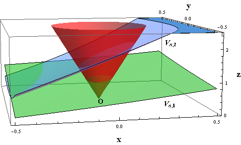
Figure 6.1: A representation of the comparison of two linear statistical hypersurfaces (in green and in blue) with an intersecting cone (in red).

The vector $\vec{X}$ is orthogonal to the normal vector $\vec{N}$ for the cone, so

$$\int_{\kappa}h\cdot(\vec{N}\cdot\vec{X})d\boldsymbol{x}=0$$ (6.6)

for any compact subset $\kappa\subseteq\mathcal{C}$ and integrable function $h$ with support $\kappa$. We can denote the boundaries $\Sigma_{1}:=V_{n,1}\cap\Omega$, $\Sigma_{2}:=V_{n,2}\cap\Omega$, and $\Sigma_{0}:=\mathcal{C}\cap\Omega$ to get a region $\Omega\subseteq\mathbb{R}^{n+1}$ with piecewise smooth boundary. The inclusion of a vanishing contribution (6.6) and a coherent choice for the orientations of the two hypersurfaces $V_{n,1}$ and $V_{n,2}$ allow us to invoke the Divergence theorem in $\mathbb{R}^{n+1}$ and get

$$\int_{\Sigma_{2}}S(\boldsymbol{x})d\boldsymbol{x}-\int_{\Sigma_{1}}S(\boldsymbol{x})d\boldsymbol{x}= \int_{\Sigma_{2}}S(\boldsymbol{x})d\boldsymbol{x}+\int_{-\Sigma_{1}}S(\boldsymbol{x})d\boldsymbol{x}$$

$$= \int_{\Sigma_{2}}S(\boldsymbol{x})d\boldsymbol{x}+\int_{-\Sigma_{1}}S(\boldsymbol{x})d\boldsymbol{x}+\int_{\kappa}\sqrt{\det\mathbf{g}}\vec{X}\cdot\vec{N}d\boldsymbol{x}$$

$$= \int_{\Omega}\nabla\cdot\vec{X}d\boldsymbol{x}^{n+1}$$

$$= \int_{\Omega}\sum_{\alpha=1}^{n+1}\frac{\partial x_{\alpha}}{\partial x_{\alpha}}d\boldsymbol{x}^{n+1}$$

$$= \int_{\Omega}(n+1)\cdot d\boldsymbol{x}^{n+1}$$

$$= (n+1)\cdot\mathrm{volume}(\Omega).$$ (6.7)

This means, once a suitable cone is given, such a compact region and its volume are well-defined, and we can associate the variation of entropy between two linear models to the volume enclosed by them.

It is worth stressing the physical meaning of this geometric construction, with reference to the two geometric objects introduced in this section, namely, the cone $\mathcal{C}$ and the integral characteristic (6.5). The cone $\mathcal{C}$ naturally arises when subsets of variables $\boldsymbol{x}$ connected by a scaling factor $k$ are considered. In more detail, in linear models the scaling $\boldsymbol{x}\mapsto(k_{B})^{-1}\cdot\boldsymbol{x}$ is related to the behaviour of the statistical hypersurface at large values of the variables, the scaling is linked to a formal variation for Boltzmann’s constant $k_{B}$, and the limit $k_{B}\rightarrow 0$ is associated with the tropical limit (of the first kind) of the statistical hypersurfaces [10] and the associated statistical amoebas [17].

For what concerns the integration step, we first note that the canonical volume form for this Riemannian manifold has been used. In turn, the metric is inherited by the ambient space $\mathbb{R}^{n+1}$. Thus, in this framework the natural emergence of an induced metric, its relation with the entropy production, and the conditions needed to apply Stokes’ theorem, are all consequences of a single principle, that is the embedding in an Euclidean space defined by the free energy (1.1).

On the other hand, different measures over $V_{n}$ may be considered. We have implicitly dealt with this aspect in the choice of an arbitrary compact subset $\Sigma$ of the statistical hypersurface $\Sigma$. In general, the introduction of a measure over the variable space associated with a probability distribution (Gibbs’ weights in our model) has a Bayesian interpretation [27]. Indeed, the parameters $\boldsymbol{x}$ defining Gibbs’ distribution $\vec{w}$ are not fixed, and the space of parameters $\mathbb{R}^{n}$ becomes a measure space with a choice of the measure $d\nu$ on it. This can be interpreted as the occurrence of parameters $\boldsymbol{x}$ with some weight expressed by the density $d\nu$, which is a typical approach in Bayesian probability. The integral (6.5) can then be seen as an “average value” for the entropy (2.9) over $\Sigma$, with weight induced by the uniform distribution over $\mathbb{R}^{n+1}$, or as the average value of the scalar product $\vec{X}\cdot\vec{N}$ with measure $\sqrt{\det\mathbf{g}}$. It is remarkable that a similar measure has been considered in information theory, i.e. Jeffreys prior [28], which is however associated with a Riemannian metric defined from the entropy, namely, the Fisher metric [29].

The introduction of different measures in (6.5) and their physical interpretation will be studied in a separate work.

6.2 Super-ideal cases

The super-ideal case where $m=n$ and $f_{\alpha}=x_{\alpha}$, $\alpha=1,\dots,n$, is a fundamental one, since it provides the basic structure for our model. On the other hand, it is also a special case, since a variation of the variables implies a variation of the functions, so the two kinds of deformations mentioned above coincide. We start from (1.4) and consider variations of the type $x_{\alpha}\mapsto x_{\alpha}+v_{\alpha}\tau$ with $\tau\ll 1$. In this way, the formula for the variation of entropy is

$$\delta S=\tau\cdot\left(\sum_{\alpha=1}^{n}w_{\alpha}x_{\alpha}\right)\cdot\left(\sum_{\beta=1}^{n}w_{\beta}v_{\beta}\right)-\tau\cdot\sum_{\alpha=1}^{n}w_{\alpha}x_{\alpha}v_{\alpha}.$$ (6.8)

The choice $v_{\alpha}=v_{\beta}$ for all $\beta=1,\dots,n$ coincides with the direction $(1,1,\dots,1)$ and satisfies the detailed balance condition $v_{\alpha}=\sum_{\beta=1}^{n}w_{\beta}v_{\beta}$. In such a case, one trivially has $\delta S=0$ since each term $\delta w_{\alpha}$ individually vanishes.

The physical requirement on the entropy growth implies a natural direction for the deformation parameter $\tau$, namely, its sign coincides with the sign for $\sum_{\alpha=1}^{n}w_{\alpha}x_{\alpha}v_{\alpha}-\left(\sum_{\alpha=1}^{n}w_{\alpha}x_{\alpha}\right)\cdot\left(\sum_{\beta=1}^{n}w_{\beta}v_{\beta}\right).$ For a given choice of $\tau$, we can consider the set of vectors $(v_{1},\dots,v_{m})$ such that $\delta S$ is non-negative. From (6.8), we can see that, for each $\boldsymbol{v}_{1},\boldsymbol{v}_{2}$ satisfying this condition, their positive combinations $c_{1}\boldsymbol{v}_{1}+c_{2}\boldsymbol{v}_{2}$ satisfy it too, and $\boldsymbol{v}$ lies in this cone if and only if $-\boldsymbol{v}$ does not. Thus, at each point $\boldsymbol{x}$, it is defined a half-space $\mathcal{H}_{\boldsymbol{x}}\subseteq\mathbb{R}^{m}$ of directions of deformations satisfying the entropy increase principle. From the previous observation, $(1,\dots,1)$ lies on the boundary of such a half-space, as can be seen from $\delta S|_{\boldsymbol{v}=(1,\dots,1)}=0$ and the linearity of (6.8) with respect to $\boldsymbol{v}$.

With reference to the integral characteristics of the kind (6.5), we can explicitly carry out its calculation for the super-ideal case at $n=2$ with variables $(x_{1},x_{2})\equiv(x,y)$. At this purpose, we choose a general rectangular domain $\Sigma:=[-c;c]\times[-c;c]$, $c>0$, and get

$$\overline{S}_{2}(c):=\int_{\Sigma}Sdxdy= \int_{\Sigma}\ln(e^{x}+e^{y})dxdy-\int_{D}\frac{e^{x}x}{e^{x}+e^{y}}dxdy-\int_{D}\frac{e^{y}y}{e^{x}+e^{y}}dxdy$$

$$= 4c\text{Li}_{2}\left(-e^{2c}\right)-6\text{Li}_{3}\left(-e^{2c}\right)-\frac{2\pi^{2}c}{3}-\frac{9\zeta(3)}{2}$$ (6.9)

where $\mathrm{Li}_{2}$, $\mathrm{Li}_{3}$, and $\zeta$ denote the dilogarithm, trilogarithm, and zeta function, respectively. From the asymptotic behaviours at $c\rightarrow+\infty$

$$\text{Li}_{2}(-e^{2c})\sim -2\cdot c^{2}-\frac{\pi^{2}}{6}+\mathcal{O}(c^{-2})+\mathcal{O}(e^{-2c}),$$ (6.10)

$$\text{Li}_{3}(-e^{2c})\sim -\frac{4\cdot c^{3}}{3}-\frac{\pi^{2}\cdot c}{3}+\mathcal{O}(c^{-2})+\mathcal{O}(e^{-2c})$$ (6.11)

the integral (6.9) increases as

$$\overline{S}_{2}(c)\sim\frac{2\pi^{2}c}{3}-\frac{9\zeta(3)}{2},\quad c\rightarrow\infty.$$ (6.12)

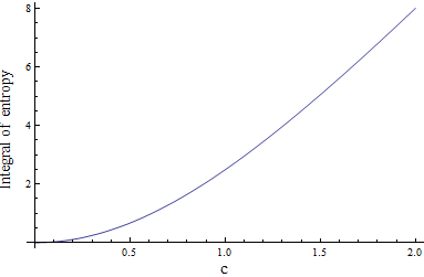
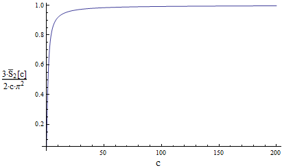
Figure 6.2: Integral of entropy for super-ideal mapping at $n=2$ over rectangular domain (a) and its ratio to the asymptotic behaviour described in (6.12) (b).

7 Conclusion

In this paper, we have discussed different connections between physical aspects of composite systems and their geometric descriptions. Main attention has been paid to the variations of the functions $f_{\alpha}$ associated with a generalized free energy and their relation with the second law of thermodynamics. Both deformations induced by a set of control variables $\boldsymbol{x}\in\mathbb{R}^{n}$, which mimic quasi-static variations within the same statistical system, and variations of the functions $f_{\alpha}\mapsto f_{\alpha}+\delta f_{\alpha}$, which change the statistical model, have been considered. The variation of associated geometric quantities (Riemann curvature tensor, Gauss-Kronecker curvature) have been provided, and a more detailed discussion on the variation of entropy has been carried out. While general variations have been considered, a characterization of the basic structure of the fundamental statistical mapping (1.1) has been given. Ideal, especially linear and super-ideal cases, have been discussed more extensively, also considering global characteristics and their interpretation in a Bayesian framework. Finally, a formulation of the stationary entropy condition in terms of discrete replicator dynamics for Gibbs’ weights has been discussed.

This study indicates the way for possible further investigations, which mainly concern the deviation from standard, equilibrium statistical models. For instance, the exploration of nonlinearities in functions $f_{\alpha}$, and their effects on Gauss-Kronecker curvature and on principal curvatures can be explored, also considering some specific physical systems that manifest non-homogeneity, small-size effects, or non-equilibrium phenomena. Likewise, the graph-theoretic interpretation of the dependence of statistical weights on functions $f_{\alpha}$ can be studied in more generality. This relates to the condition (5.15) leading to the discrete replicator equation. Thus, different weights on the graph with Laplacian (5.6), and different evolutions (5.11) may be useful to describe models out of the equilibrium.

The maximum entropy condition has played a central role in the present considerations. However, the relation with other geometric structures that describe the statistical properties of the physical system have to be investigated. In this direction, transformations acting on the statistical amoebas [17] and the effect on nonlinear deformations on the multiscale tropical limit [10] will be considered too.

Appendix A: Proof of Proposition 2

• From (5.1), we get

  $$\frac{\partial\log h_{\alpha}}{\partial f_{\beta}}=\delta_{\alpha\beta}-h_{\beta}.$$ (7.1)

  Let us define

  $$l_{\alpha\beta}:=\log h_{\alpha}-\log h_{\beta},\quad\alpha,\beta=1,\dots,m.$$ (7.2)

  At $\alpha\neq\gamma\neq\beta$ one has ${\displaystyle\frac{\partial}{\partial f_{\gamma}}l_{\alpha\beta}=0}$, so $l_{\alpha\beta}=l_{\alpha\beta}(f_{\alpha},f_{\beta})$ only depends on $f_{\alpha}$ and $f_{\beta}$. Furthermore, at $\alpha=\beta$ one has $l_{\alpha\beta}=0$, so we focus on the case $\alpha\neq\beta$. From (7.1) one easily gets

  $$\frac{\partial l_{\alpha\beta}}{\partial f_{\alpha}}=1,\quad{\displaystyle\frac{\partial l_{\alpha\beta}}{\partial f_{\beta}}=}-1,$$

  so we find

  $${\displaystyle{\displaystyle l_{\alpha\beta}=f_{\alpha}-f_{\beta}+c_{\alpha\beta}}}$$ (7.3)

  for some constants $c_{\alpha\beta}$. Clearly, $c_{\alpha\beta}=-c_{\beta\alpha}$ and

  $$0= l_{\alpha\beta}+l_{\beta\gamma}+l_{\gamma\alpha}$$

  $$= c_{\alpha\beta}+c_{\beta\gamma}+c_{\gamma\alpha}$$ (7.4)

  for all pairwise distinct $\alpha,\beta,\gamma=1,\dots,m$. Let $\sigma_{\alpha}:=c_{1\alpha}$ for all $\alpha=1,\dots,m$, where $\sigma_{1}=c_{1,1}=0$. Then $c_{1\alpha}=-c_{\alpha 1}=\sigma_{\alpha}-\sigma_{1}$ and $c_{\alpha\beta}=-c_{1\alpha}-c_{\beta 1}=c_{1\beta}-c_{1\alpha}=\sigma_{\beta}-\sigma_{\alpha}$ at $\alpha\neq 1\neq\beta$. So one has $c_{\alpha\beta}=\sigma_{\beta}-\sigma_{\alpha}$ for all $\alpha,\beta$. Thus (7.3) implies that ${\displaystyle\log h_{\alpha}-\log h_{\beta}=f_{\alpha}-f_{\beta}+\sigma_{\beta}-\sigma_{\alpha}}$. Then the quantity

  $$H:=e^{\sigma_{\alpha}-f_{\alpha}}h_{\alpha}$$ (7.5)

  is independent on $\alpha$. In order to get the compatibility of (5.1) and (7.5), one has

  $$\frac{\partial h_{\alpha}}{\partial f_{\beta}}= \delta_{\alpha\beta}H\cdot\exp(f_{\alpha}-\sigma_{\alpha})+\frac{\partial H}{\partial f_{\beta}}\exp(f_{\alpha}-\sigma_{\alpha})$$

  $$= \delta_{\alpha\beta}H\cdot\exp(f_{\alpha}-\sigma_{\alpha})-H^{2}\cdot\exp(f_{\alpha}-\sigma_{\alpha}+f_{\beta}-\sigma_{\beta})$$ (7.6)

  which implies that

  $$\frac{\partial}{\partial f_{\beta}}H^{-1}=\exp(f_{\beta}-\sigma_{\beta}).$$

  Hence one gets $H^{-1}=\exp(f_{1}-\sigma_{1})+H_{1}(f_{2},\dots,f_{m})^{-1}$ for a function $H_{1}$ of $f_{2},\dots,f_{m}$, which leads to

  $$\frac{\partial}{\partial f_{2}}\left(\frac{1}{H}\right)=\frac{\partial}{\partial f_{2}}\left[\frac{1}{H_{1}(f_{2},\dots,f_{m})}\right]=\exp(f_{2}-\sigma_{2}),$$

  so $H^{-1}=\exp(f_{1}-\sigma_{1})+\exp(f_{2}-\sigma_{2})+H_{2}(f_{3},\dots,f_{m})^{-1}$. Iterating this process, one finds $\tilde{F}:=H^{-1}=\gamma+\sum_{\alpha=1}^{m}\exp(f_{\alpha}-\sigma_{\alpha})$ where $\gamma$ is a constant, so

  $${\displaystyle h_{\alpha}=\frac{\partial\tilde{F}}{\partial f_{\alpha}}=\frac{\exp(f_{\alpha}-\sigma_{\alpha})}{\gamma+\sum_{k=1}^{d}\exp(f_{\alpha}-\sigma_{\alpha})}},\quad\alpha=1,\dots,m.$$ (7.7)

  ∎

References

• [1] G. Darboux, Leçons sur la théorie générale des surfaces et les applications géométriques du calcul infinitésimal, Vol. 1-4 (Gauthier-Villars, Paris), 1877-1896.
• [2] L. P. Eisenhart, Treatise on the differential geometry of curves and surfaces (Dover, New York), 1909.
• [3] S.-T. Yau (Ed.), Seminar on Differential Geometry, Vol. 102 (Princeton University Press, Princeton, NY), 2016.
• [4] D. R. Nelson, T. Piran and S. Weinberg (Eds.), Statistical Mechanics of Membranes and Surfaces (World Scientific, Singapore), 2004.
• [5] D. Gross, T. Piran and S. Weinberg (Eds.), Two Dimensional Quantum Gravity and Random Surfaces, Jerusalem Winter School for Theoretical Physics (World Scientific, Singapore), 1992.
• [6] F. David, P. Ginsparg and J. Zinn-Justin (Eds.), Fluctuating geometries in statistical mechanics and field theory (Elsevier-North-Holland, Amsterdam), 1996.
• [7] B. G. Konopelchenko, “Induced Surfaces and Their Integrable Dynamics”, Stud. Appl. Math. 96, 1 (1996): pp. 9–51.
• [8] B. G. Konopelchenko, and U. Pinkall, “Integrable deformations of affine surfaces via the Nizhnik-Veselov-Novikov equation.”, Phys. Lett. A 245, 3-4 (1998): pp. 239–245.
• [9] B. G. Konopelchenko, “Weierstrass representations for surfaces in 4D spaces and their integrable deformations via DS hierarchy”, Ann. Glob. Anal. Geom. 18, 1 (2000): pp. 61–74.
• [10] M. Angelelli and B. Konopelchenko, “Geometry of the basic statistical physics mapping”, J. Phys. A: Math. Theor. 49, 38 (2016): 385202.
• [11] L. D. Landau and E. M. Lifschitz, Statistical physics, Course of Theoretical Physics 5, 3 (Butterworth-Heinemann), 1980.
• [12] M. Angelelli and B. Konopelchenko, Tropical Limit in Statistical Physics, Phys. Lett. A 379, 24-25 (2015): pp. 1497–1502.
• [13] M. Angelelli, “Tropical limit and micro-macro correspondence in statistical physics”, J. Phys. A: Math. Theor. 50, 41 (2017): 415202
• [14] F. R. Gantmacher, The Theory of Matrices, Vol. I (New York, NY: Chelsea Publishing Company), 1977.
• [15] H. J. ter Horst, “Fundamental functions in equilibrium thermodynamics”, Ann. Phys. 176, 2 (1987): pp. 183–217.
• [16] H. S. Leff, “Thermodynamic entropy: The spreading and sharing of energy”, Am. J. Phys. 64, 10 (1996): pp. 1261–1271.
• [17] M. Angelelli and B. Konopelchenko, “Zeros and amoebas of partition functions”, Rev. Math. Phys. 30, 09 (2018), 1850015.
• [18] D. P. Sheehan and D. H. E. Gross, “Extensivity and the thermodynamic limit: Why size really does matter”, Physica A: Stat. Mech. Appl. 370, 2 (2006): pp. 461–482.
• [19] F. Bouchet, S. Gupta and D. Mukamel, “Thermodynamics and dynamics of systems with long-range interactions”, Physica A: Stat. Mech. Appl. 389, 20 (2010): pp. 4389–4405.
• [20] N. F. Ramsey, “Thermodynamics and statistical Mechanics at negative absolute temperatures”, Phys. Rev. 103, 1 (1956): pp. 20-28.
• [21] P. Buonsante, R. Franzosi and A. Smerzi, “On the dispute between Boltzmann and Gibbs entropy”, Ann. Phys. 375 (2016): pp. 414–434.
• [22] I. M. Bomze, “Lotka-Volterra equation and replicator dynamics: a two-dimensional classification”, Biol Cybern. 48, 3 (1983): pp. 201–211.
• [23] S. Diederich and M. Opper, “Replicators with random interactions: A solvable model.”, Phys. Rev. A 39, 8 (1989): 4333.
• [24] L. Pauling, “The structure and entropy of ice and of other crystals with some randomness of atomic arrangement”, J. Am. Chem. Soc. 57, 12 (1935): pp. 2680–2684.
• [25] E. H. Lieb, “Residual Entropy of Square Ice”, Phys. Rev. 162, 1 (1967): pp. 162–172.
• [26] H. T. Diep (Ed.), Frustrated spin sytems (Singapore: World Scientific), 2005.
• [27] M. Habeck, “Bayesian approach to inverse statistical mechanics”, Phys. Rev. E 89, 5 (2014): 052113.
• [28] H. Jeffreys, “An invariant form for the prior probability in estimation problems”, P. Roy. Soc. Lond. A Mat. 186, 1007 (1946): pp. 453–461.
• [29] S. Amari and H. Nagaoka, Methods of Information Geometry, Trans. of Mathematical monographs 191 (Oxford University Press: Am. Math. Soc.), 2000.