A Comparison of Explosion Energies for Simulated and Observed Core-Collapse Supernovae
Abstract
There are now 20 multi-dimensional core-collapse supernova (CCSN) simulations that explode. However, these simulations have explosion energies that are a few times erg, not erg. In this manuscript, we compare the inferred explosion energies of these simulations and observations of 38 SN IIP. Assuming a log-normal distribution, the mean explosion energy for the observations is () and the width is . Only three CCSN codes have sufficient simulations to compare with observations: CHIMERA, CoCoNuT-FMT, and FORNAX. Currently, FORNAX has the largest sample of simulations. The two-dimensional FORNAX simulations show a correlation between explosion energy and progenitor mass, ranging from linear to quadratic, ; this correlation is consistent with inferences from observations. In addition, we infer the ratio of the observed-to-simulated explosion energies, . For the CHIMERA set, ; for CoCoNuT-FMT, ; for FORNAX2D, , and for FORNAX3D, . On average, the simulations are less energetic than inferred energies from observations (), but we also note that the variation among the simulations (max()-min() ) is as large as this average offset. This suggests that further improvements to the simulations could resolve the discrepancy. Furthermore, both the simulations and the observations are heavily biased. In this preliminary comparison, we model these biases, but to more reliably compare the explosion energies, we recommend strategies to unbias both the simulations and observations.
keywords:
stars: massive – supernovae: general – methods: statistical1 Introduction
A primary goal of core-collapse supernovae theory is to predict which stars will explode, but for more than two decades, the more pressing challenge has been to produce at least one successful explosion in numerical simulations. Recent multi-dimensional simulations are finally producing self-consistent explosions (Lentz et al., 2015; Müller, 2015; Bruenn et al., 2016; Melson et al., 2015a; Summa et al., 2016; Radice et al., 2017; O’Connor & Couch, 2018; Ott et al., 2018; Vartanyan et al., 2018; Müller et al., 2019; Vartanyan et al., 2019; Burrows et al., 2019). While there are still only a handful of simulations with successful explosions, a trend is already emerging; the explosion energies of simulations tend to be less energetic than explosion energies inferred from observations. In this manuscript, we quantify the discrepancy between simulations and observations.
Over the last several decades, CCSN simulations have become much more computationally expensive (requiring 10s of millions of CPU-hours) but they also seem to be converging toward successful explosions. Colgate & White (1966) was the first to suggest that the change in gravitational energy due to core collapse could power the supernova explosion; they also suggested that neutrinos transfer this energy from the core to the mantle. However, more detailed modeling indicates that the bounce shock quickly stalls into an accretion shock due to electron capture and neutrino losses but mostly due to nuclear disassociation (Hillebrandt & Mueller, 1981; Mazurek, 1982). Using one-dimensional neutrino radiation hydrodynamic simulations, Wilson (1985) and Bethe & Wilson (1985) suggested that neutrinos eventually relaunch the stalled shock into an explosion. However, more modern one-dimensional simulations show that most stars do not explode. During the 1990s, two-dimensional simulations using gray flux-limited diffusion hinted that convection might aide the explosion when 1D failed (Benz et al., 1994; Herant et al., 1994; Burrows et al., 1995; Janka & Müller, 1995). Murphy & Burrows (2008) investigated the conditions for explosion and found that the neutrino luminosity required for explosion is 30% less in 2D than 1D. Mabanta & Murphy (2018) derived the conditions for explosion with and without a convection model. They found that the convection model does reduce the explosion condition by 30% in agreement with simulations, and they found that a large part of the reduction is caused by turbulent dissipation.
These investigations suggest a minimum set of requirements for self-consistent core-collapse supernova simulations. General relativity (GR) is likely important, so the code should employ GR or at least a post Newtonian potential inspired by GR. Neutrino transport should include the interactions for electron, mu, and tau flavors, and it should be multi-angle and multi-energy. Finally, the simulations should be multi-dimensional, preferably three-dimensional, but two-dimensional simulations have shown similar explosion conditions (Hanke et al., 2012) and energetics (Burrows et al., 2019). Following is a list of publications that report explosive simulations using codes with these minimum requirements: (Lentz et al., 2015; Müller, 2015; Bruenn et al., 2016; Melson et al., 2015a; Summa et al., 2016; Radice et al., 2017; O’Connor & Couch, 2018; Ott et al., 2018; Vartanyan et al., 2018; Müller et al., 2019; Vartanyan et al., 2019; Burrows et al., 2019). Of these, the following publications report positive explosion energies that begin to plateau in energy: (Müller, 2015; Bruenn et al., 2016; Melson et al., 2015a; Radice et al., 2017; Vartanyan et al., 2018; Müller et al., 2019; Vartanyan et al., 2019; Burrows et al., 2019). In general, the explosion energies reported range from 0.1 to erg.
One may infer explosion energies of observed type IIP SNe (SN IIP) by modeling the light curve and spectra of type IIP SNe (SN IIP) (Arnett, 1980). The velocity, brightness, and duration of the plateau depend mostly upon the explosion energy, ejecta mass, nickel mass, and progenitor radius (Popov, 1993; Kasen & Woosley, 2009; Dessart & Hillier, 2019; Goldberg et al., 2019). Therefore, given spectra and light curves, one may infer the explosion energy. There are two general techniques to perform this inference. One is to force explosions in one-dimensional simulations and model the expansion, spectra, and light curve (Kasen & Woosley, 2009; Sukhbold et al., 2016; Goldberg et al., 2019). In the rest of this manuscript, we refer to this as photospheric modeling. The other is to use fitting formulae to connect the photospheric parameters to model parameters (Arnett, 1980; Chugai, 1991; Popov, 1993). Generally, photospheric modeling is used to calibrate the fitting formulae. A recent investigation of photospheric modeling that also inferred explosion energies was performed by Kasen & Woosley (2009). They confirm the previous fitting formulae of Popov (1993) and very roughly infer explosion energies for SN IIP that range from 0.5 to erg.
While promising, photospheric modeling of SN IIP presents significant challenges. The most recent investigations indicate degeneracies when inferring nickel mass, ejecta mass, explosion energy, and progenitor radius (Dessart & Hillier, 2019; Goldberg et al., 2019). In fact, Goldberg et al. (2019) suggest that extra information on one of these parameters is required to break the degeneracies.
Pejcha & Prieto (2015) explored how these degeneracies affect the statistical inference of these parameters. They and Müller et al. (2017b) use the fitting formulae and statistical inference to not only infer the most likely explosion energy but also the uncertainty and covariances associated with each inference. Since they use the fitting formulae for their inference, Pejcha & Prieto (2015) caution that the inferred explosion energies may not be as precise as using the light-curve models. Instead, they suggest that their study provides a systematic investigation of the uncertainties and correlations in the inference. Later, in section 2, we demonstrate that the distribution of explosion energies from the light-curve modeling and fitting formulae are similar. Despite the concerns, this suggests that inferred explosion energies in Pejcha & Prieto (2015) may actually be as precise as the photospheric modeling results of Kasen & Woosley (2009). Since the results of Pejcha & Prieto (2015) and Müller et al. (2017b) also provide inferred uncertainties, we propose using their results to represent the inferred explosion energies for observations.
Again the explosion energies of multi-dimensional simulations range from 0.1 to erg, yet the inferred explosion energies of observations range from 0.5 to erg. This suggests that the current set of multi-dimensional simulations are less energetic than the energies inferred from observations. In this manuscript, we perform a preliminary comparison of the explosion energies of observations and multi-dimensional simulations. In section 2, we discuss the observations, compare explosion energies inferred by photospheric modeling and formula fitting, and characterize the distribution of observed explosion energies. In section 3, we describe the sample of multi-dimensional simulations. All of the simulations show a trend toward an asymptotic explosion energy, but only a few actually reach an asymptotic explosion energy. Therefore, in section 4, we propose a model for the asymptotic explosion energy and infer an extrapolated explosion energy for each simulation. Each set of simulations does not yet sample the full range of progenitors that lead to SN IIP. Therefore, in section 5, we assume a model correlating explosion energy and progenitor mass, infer the parameters of this model, and use the results to infer the full distribution of simulation explosion energies. Then we compare the simulations and observations in section 6 and infer the discrepancy between them. Finally, in section 7, we summarize and discuss how to improve the inference by addressing biases in both simulations and observations.
2 Inferred Explosion Energies from Observations
For the inferred explosion energies of observations, we consider three sources: Kasen & Woosley (2009), Pejcha & Prieto (2015), and Müller et al. (2017b). Kasen & Woosley (2009) use both light curve and spectra modeling to infer explosion energies from observations. There are more recent photospheric modeling papers (Sukhbold et al., 2016; Dessart & Hillier, 2019; Morozova et al., 2018; Goldberg et al., 2019). However, three of these do not actually infer explosion energies that are based upon observations; their focus is on providing better models and understanding the degeneracies (Sukhbold et al., 2016; Dessart & Hillier, 2019; Goldberg et al., 2019). Morozova et al. (2018) do attempt to infer explosion energies. However, their inference is based upon light curve modeling alone, and does not include the important velocity constrains provided by spectra. Given that there are significant degeneracies among the model parameters, it is important to include all observational constraints (Dessart & Hillier, 2019; Goldberg et al., 2019). The other two sources that we consider, Pejcha & Prieto (2015) and Müller et al. (2017b), use statistical inference methods to infer the explosion energy, nickel mass, and ejecta mass for 38 Type II-Plateau supernovae. See Table 1 for the list of SNe. To infer these model parameters, they used , the absolute V band magnitude, , the duration of the optically thick plateau phase, and , the expansion velocity of the photosphere. Both and were evaluated at the midpoint of the plateau phase. In their likelihood model, the explosion parameters are related to these observations via analytic scalings that were calibrated using one-dimensional radiation-hydrodynamic explosion models. These models do not simulate the explosions self-consistently. Rather, they force the explosions, and relate the simulated light curve and expansion velocity to the forced explosion energy, ejecta mass, and nickel mass.
To date, the inferences of Pejcha & Prieto (2015) and Müller et al. (2017b) represent the most thorough analysis of the uncertainty and covariances for the explosion parameters. On the other hand, Pejcha & Prieto (2015) also caution that the mode of their inferences may not be as reliable as inferences based upon numerical modeling of light curves. However, as yet, there are no statistical inferences using numerical modeling. Therefore, to assess the accuracy of the Pejcha & Prieto (2015) and Müller et al. (2017b) statistical inferences, we compare their distribution of explosion energies with the distribution from Kasen & Woosley (2009), who model the light curve and expansion velocities. Kasen & Woosley (2009) do not present a formal inference. However, in the right panel of their Figure 16, they compare explosion energy as a function of photospheric velocity and . On the same figure, they present observations for 22 SNe. From this figure, we create a fitting function for the explosion energy and use this to simply infer the explosion energy for each SN. Note that this is not a thorough statistical inference, just simple inference using a fitting formula.
Figure 1 compares the distributions of explosion energies for the two samples: one based upon photospheric modeling (Kasen & Woosley, 2009); the other is based upon fitting formulae (Pejcha & Prieto, 2015; Müller et al., 2017b). The KS test gives a D statistic of 0.22 and a P-value of 0.44. The two distributions are consistent with being drawn from the same distribution. Even though Pejcha & Prieto (2015) suggest that the precision of their inference may not be as good as the simulations of Kasen & Woosley (2009), we find that they are actually in agreement. Since the Pejcha & Prieto (2015) and Müller et al. (2017b) inference provides both an explosion energy and an uncertainty, we use their inferred explosion energies for the observational set.
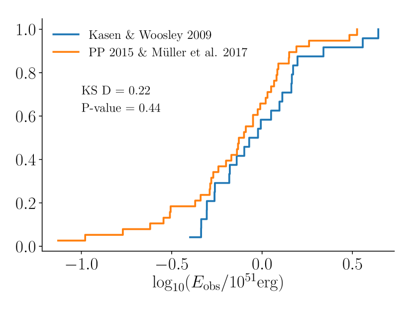
Figure 2 of Pejcha & Prieto (2015) gives their posterior distributions for Ni mass and explosion energy. At the moment, we are only concerned with the explosion energy, so we use the results in that figure to estimate the marginalized posterior distributions for explosion energy. We model their distributions as a log normal; Table 1 provides the mode and uncertainties for the explosion energies.
| Name | ||
|---|---|---|
| SN 2001dc | -1.13 | 0.33 |
| SN 2013am | -0.98 | 0.25 |
| SN 1980K | -0.77 | 0.27 |
| SN 1995ad | -0.62 | 0.23 |
| SN 2005cs | -0.55 | 0.21 |
| SN 2009js | -0.51 | 0.43 |
| SN 2009dd | -0.29 | 0.46 |
| SN 2012A | -0.28 | 0.10 |
| SN 2009N | -0.24 | 0.15 |
| SN 2009bw | -0.20 | 0.13 |
| SN 2004A | -0.13 | 0.28 |
| SN 2008in | -0.13 | 0.60 |
| SN 2004dj | -0.14 | 0.23 |
| SN 2004et | -0.02 | 0.16 |
| SN 1996W | 0.07 | 0.28 |
| SN 2012aw | 0.08 | 0.16 |
| SN 1999em | 0.15 | 0.15 |
| SN 2008bk | 0.48 | 0.53 |
| SN 1992H | 0.53 | 0.29 |
| SN 1992ba | -0.09 | 0.21 |
| SN 2002gw | 0.08 | 0.12 |
| SN 2003B | -0.37 | 0.23 |
| SN 2003bn | -0.01 | 0.09 |
| SN 2003E | 0.09 | 0.14 |
| SN 2003ef | 0.19 | 0.10 |
| SN 2003fb | 0.03 | 0.14 |
| SN 2003hd | 0.05 | 0.08 |
| SN 2003hn | -0.34 | 0.12 |
| SN 2003ho | 0.26 | 0.10 |
| SN 2003T | -0.05 | 0.09 |
| SN 2009ib | -0.27 | 0.08 |
| SN 2012ec | -0.10 | 0.06 |
| SN 2013ab | 0.02 | 0.20 |
| SN 2014ej | -0.05 | 0.12 |
| SN 2013fs | -0.29 | 0.08 |
| SN 2014G | -0.17 | 0.08 |
| ASASSN-14gm | 0.15 | 0.11 |
| ASASSN-14ha | -0.51 | 0.16 |
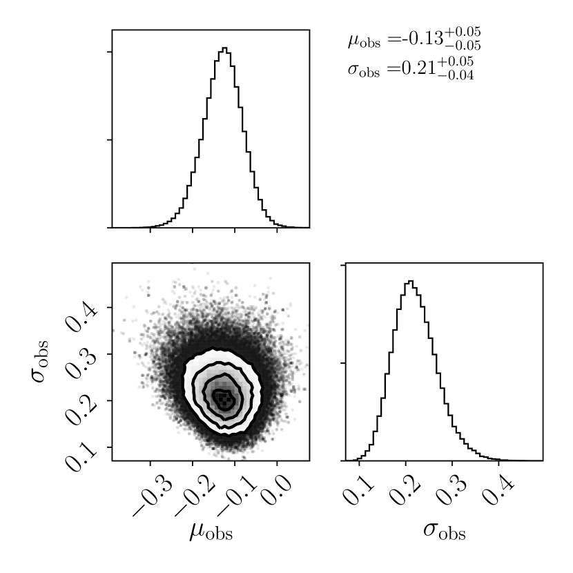
Next, we infer the distribution of observed explosion energies by modeling the mean () and width () of the observations. For a rough estimate, one may calculate the mean and variance of the modes (2nd column in Table 1). However, when the uncertainties in the observations are large, these estimates can easily be biased. In particular, the observed variance in the distribution is a convolution of the true width and the large uncertainties, so simply calculating the variance of the observations will lead to an over estimation of the width. Therefore, we use Bayesian inference to infer the distribution of explosion energies.
The posterior distribution is
| (1) |
where and are uniform priors. The likelihood for each observation is
| (2) |
To infer this posterior distribution, we use the Markov Chain Monte Carlo package emcee (Foreman-Mackey et al., 2013); Figure 2 shows the posterior distribution for the model parameters; the mode and the 68% highest density intervals (HDI) are and . The mean corresponds to an energy of erg.
3 Inferred Explosion Energies from CCSN Simulations
To simulate the core-collapse problem with some fidelity, CCSN simulations must include the following physics: multi-dimensional hydrodynamics, general relativity, dense nuclear equations of state (EOS), weak interactions, nuclear reactions, and neutrino transport. Codes that simulate all of these physics with any fidelity are computationally expensive. For example, current three-dimensional neutrino radiation hydrodynamics simulations require 10s of millions of CPU-hours; on 10,000 cores or more this requires months of computational time for just one run. As a result most codes make some approximations. Even the most advanced codes require some approximations. For the purpose of this study, we only select simulations that meet the following minimum approximations. Gravity should include at least a pseudo GR spherical potential. The neutrino transport should be a self-consistent approximation of the Boltzmann equation. Two examples of such neutrino transport are 1) solving the Boltzmann equation using discrete methods along rays, and 2) solving moment equations. The transport also should be multi-species, multi-group, and multi-angle in its approximation. The individual simulations should also show signs of approaching a final explosion energy.
The codes that satisfy these technical requirements are CHIMERA, CoCoNuT-FMT, FORNAX, PROMETHEUS-VERTEX, Zelmani, FLASH, and the Kuroda et al. (2016) code. However, not all of these have simulations that explode and asymptotically approach a final explosion energy. Only simulations using CHIMERA, FORNAX, and CoCoNuT-FMT satisfy all conditions. The following is a brief description of each code, including references that include the simulation sets.
3.1 Codes and Simulation Sets Included in This Study
CHIMERA: The full code architecture and capabilities are presented in Bruenn et al. (2006); Messer et al. (2007, 2008); Bruenn et al. (2009, 2013). The hydrodynamics solver is a dimensionally-split, Lagrangian-plus-remap Newtonian scheme with piece-wise parabolic reconstruction. Self-gravity is computed by a multi-pole expansion and the neutrino transport is computed using ray-by-ray, with multi-group flux limited diffusion (MGFLD) as the transport solver. The simulations of Bruenn et al. (2016) use the MeV incompressibility version of the Lattimer & Douglas Swesty (1991) EOS for densities g cm-3.
Using two-dimensional simulations, Bruenn et al. (2016) report explosions of the 12, 15, 20, and 25 M⊙ progenitors of (Woosley & Heger, 2007). Lentz et al. (2015) report the explosion of the 15 M⊙ progenitor in three-dimensional simulations. With only one three-dimensional simulation, it is difficult to explore the trends and systematics with mass, etc. Furthermore, the simulation ends after 440 ms past bounce and 140 ms past the initiation of positive diagnostic explosion energies. The explosion energy does not start to plateau, and thus our extrapolation model for late times would be invalid in this case. Therefore, we restrict the CHIMERA sample to the 2D simulations of Bruenn et al. (2016).
CoCoNuT-FMT: The primary description of this code’s architecture is in Müller (2015). The latest advancements for this code are in Müller et al. (2019). The hydrodynamics solver for CoCoNuT-FMT solves the general relativistic hydrodynamics in spherical coordinates on a unsplit finite-volume mesh. Fluxes are calculated using an HLLC Riemann solver, and the metric equations are solved in the extended conformal flatness approximation with a spherically symmetric metric. The neutrino transport is multi-group and uses a variable Eddington factor closure and solves the transport using ray-by-ray. The transport includes gravitational redshift but neglects both velocity dependent terms and inelastic scattering. However, there is a Doppler correction to the absorption opacity.
In a three-dimensional simulation, Müller (2015) report the explosion of the 11.2-M⊙ progenitor of Woosley et al. (2002); for this simulation, Müller (2015) employ the MeV version of the Lattimer & Douglas Swesty (1991) nuclear EOS. Using Coconut-FMT and a 3D 18-M⊙ initial progenitor to provide perturbations, Müller et al. (2017a) produced a perturbation-aided explosion. Most recently, Müller et al. (2019) produced several explosions of progenitors with zero-age main sequence (ZAMS) masses between 9.6 M⊙ and 12.5 M⊙. Since the Müller et al. (2019) study probes a sufficiently high resolution of the mass space, we choose the diagnostic energies from this set of simulations for our examination. Since there is only one model that explores perturbation-aided explosions, we do not include the results of 18-M⊙ simulation (Müller et al., 2017a) in the final comparison with observations. However, in section 7, we do discuss the possible implications of perturbations on explosion energies in simulations.
FORNAX: The technical details and capabilities of FORNAX are presented in Skinner et al. (2018). In summary, this code solves both hydrodynamics and radiation transport using explicit, finite volume Godunov schemes. For gravity, they use a multi-pole solver and replace the monopole part of the potential with a post-Newtonian approximation for GR. The transport algorithm is a multi-group, two-moment closure scheme and uses the M1 moment closure for the Eddington tensor. Both the hydro and the transport components calculate the fluxes between cells using approximate Riemann solvers. Because the transport is explicit, the time step is limited by the speed of light across the zone. In general, the speed of sound in the protoneutron star is 1/3 the speed of light, so calculating the neutrino transport explicitly only increases the number of time steps by a factor of 3. The reductions in calculations for an explicit transport solver versus an implicit solver more than compensate for this increase in speed. In general, simulations involving FORNAX use either the MeV version of the Lattimer & Douglas Swesty (1991) EOS or the SFHo EOS (Steiner et al., 2013) dense nuclear equations of state.
There are four primary publications that report CCSN explosions in FORNAX simulations. We divide them into two sets, two-dimensional simulations, FORNAX2D, and three-dimensional simulations, FORNAX3D. Radice et al. (2017) explored explodability of two-dimensional simulations for the following progenitors: n8.8, u8.1, z9.6, 9.0, 10.0, 11.0. The numbers in these models represent the zero-age main sequence mass. All models use the K=220 MeV version of the Lattimer & Douglas Swesty (1991) EOS; they also explode in both one-dimensional and two-dimensional simulations. Vartanyan et al. (2018) simulated collapse of the 12, 13, 15, 16, 17, 19, 20, 21, and 25 M⊙ progenitors (Woosley & Heger, 2007). For these simulations, they use the SFHo EOS (Steiner et al., 2013). They reported explosions for the 16, 17, 19, and 20 M⊙ progenitors, but only the 16, 17, and 19 M⊙ progenitors provide diagnostic explosion energies that are greater than zero and approach an asymptotic value. Vartanyan et al. (2019) simulated three-dimensional collapse and explosion of the 16 M⊙ progenitor. They find an explosion, but this simulation has yet to reach positive diagnostic explosion energies. More recently, Burrows et al. (2019) simulate the three-dimensional explosions for the same 9, 10, 11, 12, and 13 M⊙ progenitors but using the SFHo EOS (Steiner et al., 2013). For the progenitors that are simulated both in two and three dimensions, the explosion time and diagnostic explosion energies are very similar.
3.2 Codes and Simulations Not Included in this Study
PROMETHEUS-VERTEX: Melson et al. (2015a) describe the code architecture for this code. The hydrodynamics algorithm is a finite volume Godunov scheme using Riemann solvers to calculate fluxes. For gravity, the code solves the multi-pole expansion and replaces the monopole with a pseudo potential that represents a post-Newtonian approximation to GR. The neutrino transport solves the Boltzmann equation on radial rays.
There are two three-dimensional explosions using Prometheus-Vertex. Melson et al. (2015a) report the three-dimensional explosion of a 9.6 M⊙ star. In the same year, Melson et al. (2015b) report the three dimensional explosion of a 20 M⊙ star. These represent the first self-consistent three-dimensional explosions. However, the latter is not what one would consider a fiducial simulation; it explores strange-quark contributions to the neutrino-nucleon scattering. The former does explode and begins to approach asymptotic values at about 400 ms past bounce or 300 ms past the initiation of explosion. The final reported explosion energy is erg, and the final rate of increase is about erg s-1. Summa et al. (2016) simulated the explosion of 18 progenitors in two-dimensional simulations. However, they only reported diagnostic explosion energies for 4 of the progenitors, and these did not reach asymptotic values in the explosion energy. With only one simulation reaching the final phase of the explosion, it is difficult to make any systematic conclusions about the performance of Prometheus-Vertex simulations. Therefore, we do not include Prometheus-Vortex results at this time.
FLASH: O’Connor & Couch (2018) include approximate GR in FLASH, a finite-volume hydrodynamics code. The gravity algorithm solves the Newtonian Poisson’s equation via a multi-pole solver and replaces the monopole term with a post-Newtonian pseudo GR potential. The neutrino transport solves the two-moment equations and uses the M1 closure. The transport is also multi-group, includes velocity dependence and inelastic scattering.
Using FLASH, O’Connor & Couch (2018) simulated the collapse of the 12, 15, 20, and 25 M⊙ progenitors (Woosley & Heger, 2007). The 15, 20, and 25 M⊙ runs exploded, reaching explosion energies ranging from 0.15 to erg. However, none reach the plateau phase in diagnostic explosion energy, so we are not able to include these results in our comparison.
Zelmani: Roberts et al. (2016) present the code architecture. Zelmani is a three-dimensional GR, multi-group radiation-hydrodynamics code. The neutrino transport solves the two-moment equations and uses an M1 closure. Zelmani also neglects velocity dependence and inelastic scattering processes. Ott et al. (2018) simulated the explosions of 12-, 15-, 20-, 27-, and 40-M⊙ progenitor models of Woosley & Heger (2007) and with the SFHo (Steiner et al., 2013) EOS. Though the fidelity of this code meets the requirements of our analysis, the simulations terminated very shortly after explosion, and so the explosion curves are far from their plateau phase. Thus, we are not able to include these simulations in this study.
Kuroda (2016): The code presented in Kuroda et al. (2016) meets some of the technical requirements. The neutrino transport is multi-group and is a two-moment scheme using the M1 closure. The code solves the GR field equations. They simulated collapse of a 15 M⊙ progenitor. However, this simulation did not explode.
4 Extrapolating Simulated Explosion Energies to Late Times
The explosion energies in many of the multi-dimensional simulations are still increasing when the simulations terminate. At the same time, most appear to be approaching an asymptotic value. Therefore, at best, the reported diagnostic explosion energies are a minimum. Here, we note that the energy evolution for all simulations follows a common functional form. We suggest a simple model for explosions driven by neutrino heating. This model leads to a simple functional form that is a good fit to the simulations. Here we use this functional form to extrapolate the explosion energy to infinite time, .
Figure 3 shows the diagnostic explosion energies in units of erg as a function of time after bounce. The solid lines represent the results of multi-D simulations, and the bands at the end of each curve represents our extrapolation. Blue represents CHIMERA simulations, green represents CoCoNuT-FMT, brown represents FORNAX2D, and yellow represents FORNAX3D. All curves rise and show signs of asymptotically approaching a finite explosion energy, . In a preliminary analysis, we considered two functional forms: an exponential and a power-law. These crude initial comparisons suggests that the energy curves asymptote via a power-law and not an exponential. Using this crude analysis as a guide, we now suggest a model for the explosion energy curve and derive the functional form.
If neutrinos are primarily driving the explosion, then one might expect the rate of growth of explosion energy to be roughly proportional to the neutrino power.
| (3) |
where is the neutrino luminosity and is the optical depth to neutrino absorption in the region of net neutrino heating. is the neutrino absorption cross section per unit mass, .
A few straightforward assumptions lead to a simple function for . First, during the explosion, we assume that the optical depth is roughly , where is the mass in the gain region and and is the shock radius. Making the simplest assumptions, we assume that and are roughly constant during the last stage of explosion development. In addition, we assume that , and that the shock velocity, is also constant. Integrating eq. (3) leads to the following functional form
| (4) |
Formally, is proportional to , but we do not have access to these values for all of the simulations. Therefore, in our extrapolations, we fit only for two parameters, and .
We use Bayesian inference to find the best fit values for and . The posterior distribution for and is
| (5) |
It is unclear what the variance is for the simulations. Therefore, we include as an unknown nuisance parameter and simply marginalize over all possible values to infer the posterior distribution for and , . With little prior information about any of these parameters, we choose uniform priors for , , and . To model the likelihood, we assume a Gaussian distribution for each simulation data point:
| (6) |
where
| (7) |
The mean is the modeled explosion energy, eq. (4). The unknowns to infer are the asymptotic explosion energy, , the parameter for the term, , and the unknown variation within each simulation, .
When inferring these parameters, we only fit the last half of the energy curve. The primary assumptions of the evolution model assume that , , and are constant. If these assumptions are appropriate at all, they are likely valid in the last part of the explosion energy evolution. To perform these inferences, we use Markov Chain Monte-Carlo Bayesian inference package emcee (Foreman-Mackey et al., 2013). The bands extrapolating the energy curves in Figure 3 show the resulting inferences. The width of the band represents the 68% highest density confidence interval (HDI) for these fits.
Table 2 summarizes the set of simulation explosion energies. The first row gives the progenitor as presented in the simulation papers. Each progenitor name conveniently indicates the ZAMS mass in M⊙. The second column reports the final explosion energy of the simulation, . The third column presents the end of the simulation in seconds after bounce, . Finally, column four shows the mode of the extrapolated explosion energy, .
| Progenitor | [ erg] | [s] | [ erg] |
|---|---|---|---|
| CHIMERA | |||
| 12 | 0.31 | 0.97 | 0.34 |
| 15 | 0.88 | 0.81 | 1.03 |
| 20 | 0.38 | 0.84 | 0.50 |
| 25 | 0.70 | 0.73 | 0.93 |
| CoCoNuT-FMT | |||
| 11.2 | 0.13 | 0.77 | 0.16 |
| s11.8 | 0.20 | 0.78 | 0.24 |
| s12.5 | 0.16 | 0.90 | 0.19 |
| z12 | 0.41 | 1.68 | 0.47 |
| z9.6 | 0.13 | 0.12 | 0.18 |
| 18ProgConv | 0.77 | 1.96 | 0.98 |
| FORNAX2D | |||
| 11.0 | 0.11 | 0.98 | 0.15 |
| 9.0 | 0.06 | 0.98 | 0.08 |
| n8.8 | 0.18 | 0.51 | 0.19 |
| u8.1 | 0.10 | 0.85 | 0.11 |
| z9.6 | 0.12 | 0.58 | 0.13 |
| 16 | 0.16 | 1.13 | 0.21 |
| 17 | 0.29 | 0.90 | 0.39 |
| 19 | 0.24 | 0.52 | 0.39 |
| FORNAX3D | |||
| 9.0 | 0.10 | 0.91 | 0.11 |
| 10.0 | 0.03 | 0.62 | 0.04 |
| 11.0 | 0.09 | 0.44 | 0.12 |
| 12.0 | 0.09 | 0.54 | 0.12 |
The four panels in Figure 4 compare with an estimate for the observed explosion energies. The vertical lines indicate the estimated simulation explosion energy. The height of the lines are proportional to , representing the initial mass distribution. In other words, the height represents the fraction of stars that would explode with that energy within the simulated set. The gray lines in each represent the “marginalized” inferred explosion energies from observations (Pejcha & Prieto, 2015). The term marginalized is in quotes because without the original posterior distributions, we performed a crude marginalization using Figure 2 from Pejcha & Prieto (2015). The fraction in each figure represents the fraction of the IMF that each code has simulated from 7.4 to 25 M. The minimum corresponds to the minimum mass for CCSNe (Díaz-Rodríguez et al., 2018), the maximum corresponds to the maximum mass for SN IIP (Smartt, 2015; Davies & Beasor, 2018). For further discussion on these limits see section 7.
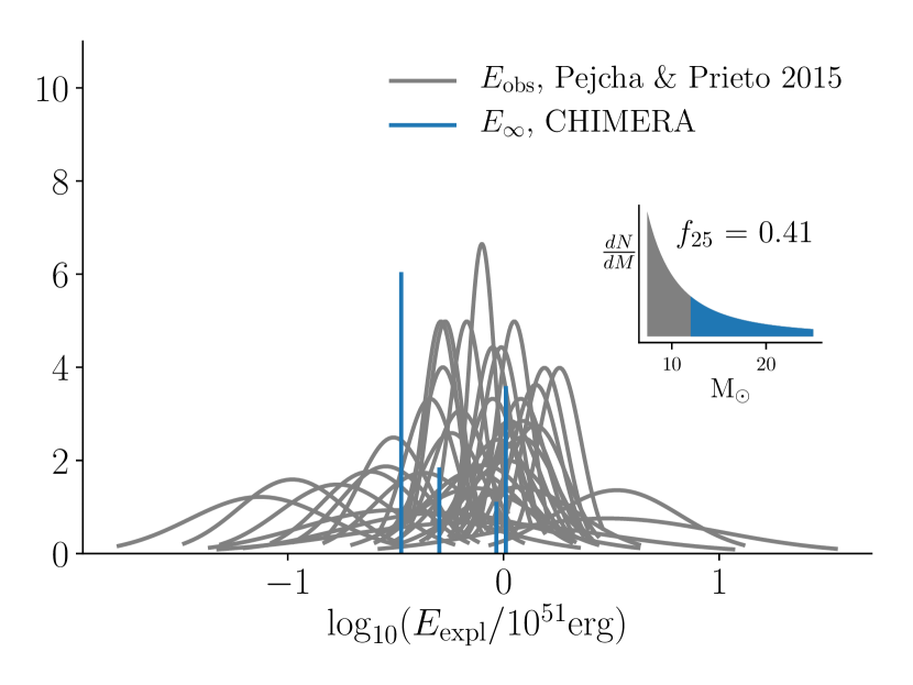
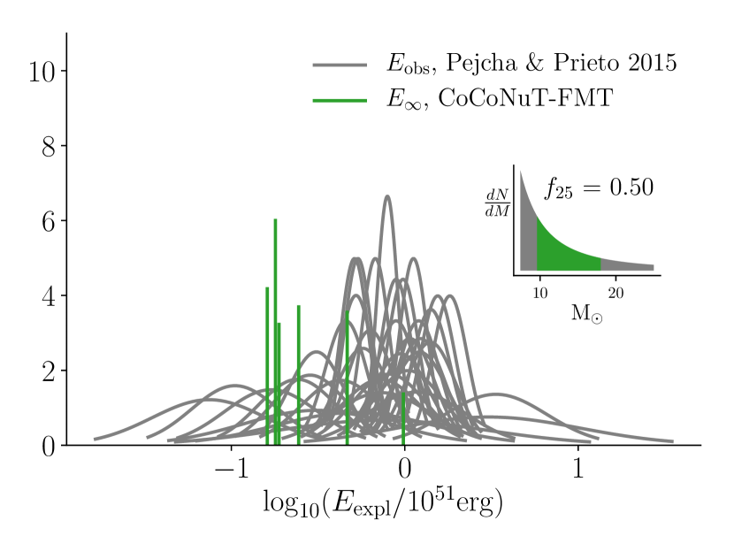
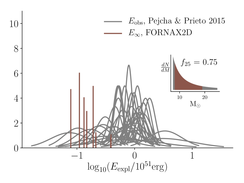
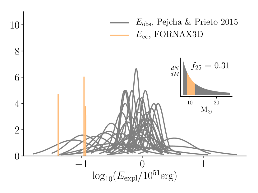
Upon first glance, the CHIMERA set appears to be most consistent with the observations, and the FORNAX sets are the least consistent. However, the CHIMERA simulations mostly use the highest mass progenitors. Below, we note a correlation between explosion energy and progenitor mass for the FORNAX2D set. Therefore, the CHIMERA results may actually represent the highest explosion energies when a full range of progenitors are considered. In other words, the range of progenitor masses simulated represents a possible bias for each simulation set. Below, we model the explosion energy as a function of progenitor mass to account for this possible bias.
5 Inferring the Full Simulation Explosion Energy Distribution
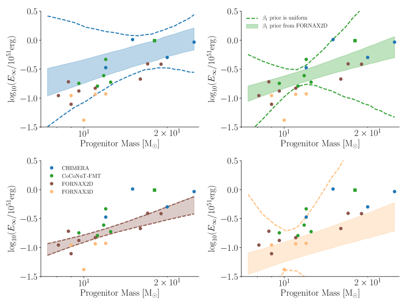
The simulation sets have not yet sampled the whole range of progenitors from 7.4 to 25 M⊙. Therefore, the explosion energies in Table 2 represent a biased sample. For example, Figure 5 plots (dots) vs. progenitor mass. It is apparent that the CHIMERA set includes mostly high mass progenitors, the CoCoNuT-FMT set includes mostly the middle, and the FORNAX2D set has simulated a larger range. Note that the 18ProgConv model (green square) is omitted in the analysis for CoCoNuT-FMT. In this section, we infer a relationship between explosion energy and progenitor mass. Then we use this inference to infer the full distribution of explosion energies between 7.4 and 25 M⊙.
The simplest assumption is that the explosion energy is proportional to some power of the progenitor mass. In fact, for SN IIP observations Pejcha & Prieto (2015) infer that the explosion energy is proportional to a power of the ejecta mass, . Therefore, the most natural model to assume for the correlation is
| (8) |
To infer the parameters, and , we use emcee (Foreman-Mackey et al., 2013) to infer the following posterior distribution
| (9) |
where the likelihood for the simulated explosion energy is
| (10) |
The variation in the simulated energies, , is an unknown nuisance parameter. The priors, , , and , are all assumed to be uniform.
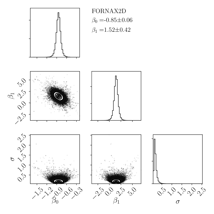
Figure 6 shows the posterior distribution for the FORNAX2D simulation set. The marginalized parameters are and . The values are the modes, and the uncertainties are the 68% highest density intervals (HDI). For the CHIMERA, CoCoNuT-FMT, and FORNAX3D simulation sets, there are far too few simulations to adequately constrain the slope. Therefore, we use the distribution for FORNAX2D as the prior for the other two sets. The marginalized parameters for CHIMERA are and ; the marginalized parameters for CoCoNuT-FMT are and ; the marginalized parameters for FORNAX3D are and . The inference for CoCoNuT-FMT does not include the 18ProgConv model. The lines in Figure 5 represent the distribution of possible functions. For each MCMC sample of and , we calculate as a function of . Then we calculate the 68% HDI for . Within the confidence intervals, the exponent ranges from linear to quadratic, .
Using observations, Pejcha & Prieto (2015) infer the relationship between the explosion energy ( in their manuscript) and the ejecta mass . Since the neutron star that is left behind is only 1.4 M⊙, and there is not much mass loss for the red supergiant progenitors they consider, the ejecta mass is similar to the ZAMS progenitor mass. They find that , which is consistent with our inference.
Next, we extrapolate to infer the explosion energy distribution for the range of progenitor masses between 7.4 and 25 M⊙. The posterior for the explosion energies is
| (11) |
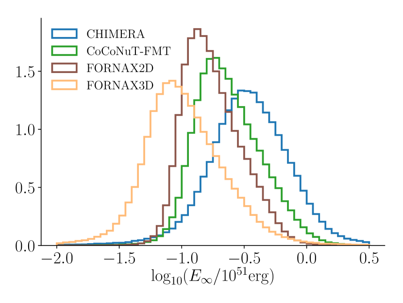
where is the posterior distribution, eq. (9), for the model parameters, and is the progenitor mass distribution. For this study, we assume that . To determine , we take a sample of from MCMC posterior distribution, draw a mass from the IMF distribution, , and evaluate using eq. (8). The resulting distributions for each code are in Figure 7. On average, all simulations sets exhibit explosion energies that are significantly lower than the observations. In the next section, we quantify the difference between simulations and observations.
6 Comparing Observations with Multidimensional Simulations
Since the average explosion energies of the simulations are lower than the observations, we develop a model to infer the missing explosion energy, . For compactness and readability in the following equations, we define . The posterior distribution for is
| (12) |
We assume a uniform prior for , . This posterior distribution represents a hierarchical Bayesian inference where and are intermediate nuisance parameters. The portion of the likelihood that is has already been calculated and is shown in Figure 7. Since the distributions for are essentially Gaussian, we use the Gaussian approximation for . With this approximation, the marginalization over the nuisance parameters in eq. (12) is analytic, and the likelihood is now given by
| (13) |
where is the mode of , and is the half width of the 68% HDI.
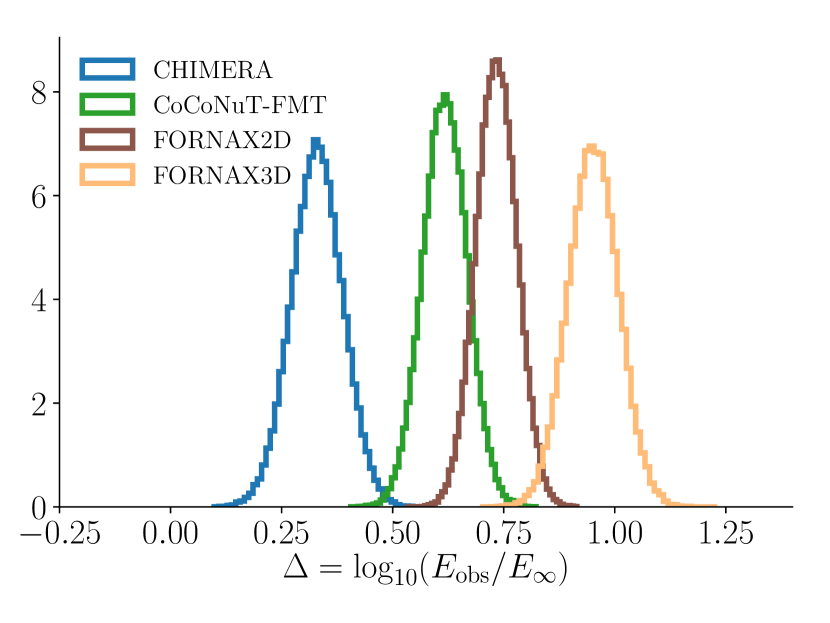
Figure 8 shows the inferred distributions for the four simulation sets. For CHIMERA, ; for CoCoNuT-FMT, ; for FORNAX2D ; for FORNAX3D . All three simulations set have more than 99.9% of their distributions, , greater than zero. Based upon the models and assumptions in this manuscript, all three simulation sets have explosion energies that are significantly smaller than observations. In the best case (CHIMERA), the simulated explosion energies are a factor 2 less energetic than the observed energies. In the worst case (FORNAX3D), the simulated explosion energies are a factor of 10 less energetic.
7 Discussion & Conclusions
In general, we find that the explosion energies of multi-dimensional simulations are significantly less energetic than the explosion energies inferred from observations. For this comparison, we require the CCSN simulations and codes to have the following attributes; two- or three-dimensional, neutrino transport that is a self-consistent approximation of Boltzmann transport equations, transport is multi-angle and multi-species, general relativity or some post-Newtonian approximation, and positive explosion energies, approaching asymptotic values. The codes that satisfy these requirements are CHIMERA, CoCoNuT-FMT, and FORNAX. For the observational explosion energies, we use the results of Pejcha & Prieto (2015) and Müller et al. (2017b), who infer the explosion energies, uncertainties, and correlations for 38 type IIP supernovae. We infer a mean observational explosion energy of in units of ; the width of the distribution is . To compare the observations and simulations, we infer the ratio of observed-to-simulated explosion energies, , where is our estimate of the simulation energy extrapolated to infinite time. For CHIMERA, , for CoCoNuT-FMT, , for FORNAX2D, , and for FORNAX3D, . Overall, all simulation sets are less energetic than the explosion energies inferred from observations.
This result suggests a tension between the simulations and observations. However, it does not yet rule out the standard neutrino mechanism. Of the four simulation sets, the mean offset is , but the range goes from 0.33 to 0.95, and the width of this range is 0.6. In other words, the variance among different simulation sets is of order the average offset. Given this, it is plausible that future improvements to the simulations might resolve the current discrepancy.
In this analysis, we identify several biases in the simulation sets. Core-collapse simulations are computationally expensive, and few of the results include large systematic studies of the full range of progenitors. Furthermore, most simulations terminate well before an asymptotic explosion energy.
To mitigate for these biases in the simulation sets, we model the distribution of explosion energies from simulations. The FORNAX2D results exhibit the largest sample, so we use their results to infer an explosion energy vs. progenitor mass relationship. Our inference shows that ; the simulation explosion energies are proportional to progenitor mass with a power ranging from linear to quadratic. To infer the simulation explosion energy after infinite time, we fit a simple model, , that is motivated by a simple neutrino-powered explosion. Then we assume that all models between the 7.4 M⊙ and 25 M⊙ explode. This range includes the minimum mass for CCSN explosions (Díaz-Rodríguez et al., 2018) and a rough estimate for the maximum progenitor for SN IIP (Smartt, 2015; Davies & Beasor, 2018).
Better estimates for the simulated explosion energy distribution will require more systematic explorations between 7.4 and 25 M⊙, and better estimates will require simulations that terminate later. Based upon our simple model, simulations must evolve roughly 0.5 to 2 seconds past the time of positive explosion energies to reach at least 90% of the asymptotic explosion energy.
There are other potential biases in the simulations which are either difficult to quantify in this study or have yet to be identified at all. For example, resolution of the grid may impact whether CCSN simulations have converged. Recently, Melson & Janka (2019) explore how resolution affects turbulence in simplified three-dimensional CCSN simulations, but these explorations do not address how resolution affects the explosion energies. A major difference among the codes is the treatment of neutrino transport. There are many approximations and choices in the transport: ray-by-ray vs. multi-angle, energy groups, moments vs. short characteristics, moment closures, velocity-dependent terms, gravitational redshift, scattering opacities, correlated opacities, etc. In fact, there are more different choices in the neutrino transport treatment than there are codes. Yet, it is unclear how these differences impact the explosion energies.
Progenitor perturbations due to O-shell burning may be important in reducing the tension between simulations and observations. The majority of simulations that are available do not include progenitor perturbations, but the one model that does, offers some tantalizing clues. The 18ProgConv model of the CoCoNuT-FMT set has the largest explosion energy of that set. If we include this one model, then the discrepancy reported for CoCoNuT-FMT does not actually change much. The lack of change is because this model has a relatively high mass. The explosion energy vs. progenitor mass correlation already indicates that the higher masses explode with higher energy. Including 18ProgConv in the fit only steepens the dependence a little. In addition, the highest masses are more rare and provide little weighting to the final explosion energy distribution. So, this one perturbation-aided explosion does not change for CoCoNuT-FMT.
However, it is not clear what progenitor perturbations would do for the lower mass progenitors. Müller et al. (2017a) report a difference in explosion time depending upon the size of the progenitor perturbations. They simulated three 18-M⊙ progenitors models: one with no O-shell perturbations, one with a convective mach number of 0.04, and one with a convective mach number of 0.1. The first did not explode by 650 ms after bounce, the second exploded at around 500 ms, and the largest perturbations exploded at 300 ms. They only show the inferred explosion energy for the largest perturbations, so we do not have a quantitative measure of how perturbations affect the explosion energy. None the less, an earlier explosion might lead to higher explosion energies. To test whether progenitor perturbations affect the explosion energies, we recommend that simulators perform a systematic study of progenitor perturbations for a wide range of masses.
Throughout this manuscript, we are careful to note that the explosion energies that represent the observations are not observations in themselves, but are inferences based upon observations. As such, the “observed” explosion energies are also subject to biases. The observational explosion energy set relies on modeling type IIP light curves and spectra. Currently, there are two general approaches. One is to use one-dimensional radiation hydrodynamic simulations to model the light curve and spectra (Kasen & Woosley, 2009). The second is to use fitting formulae to infer explosion energies, etc (Pejcha & Prieto, 2015; Müller et al., 2017a). The modeling efforts are potentially more accurate, but the fitting formulae are more amenable to statistical inference and better uncertainty estimates. For this preliminary analysis, we find the distribution of explosion energies from light curve modeling and fitting formulae to be consistent. Therefore, we use the statistical inference results from the fitting formulae. A more accurate and precise estimate would be to use the light curve models in a statistical inference framework.
A significant source of systematic uncertainty in modeling the photospheric properties is the zero point in the fitting formulae. Goldberg et al. (2019) summarize the zero points for several studies (Popov, 1993; Kasen & Woosley, 2009; Sukhbold et al., 2016; Goldberg et al., 2019); see the discussion just after eq. (7) in their manuscript. They find that the systematic uncertainty in the luminosity zero points is about 0.09 in log base 10. This translates to a systematic uncertainty in the log of the explosion energy of 0.1. While this is not enough to completely account for the discrepancy between the simulations and observations, it is of the same order. In addition, Dessart & Hillier (2019) and Goldberg et al. (2019) caution that there are significant degeneracies among the explosion parameters: nickel mass, ejecta mass, explosion energy, and progenitor radius. In fact, Goldberg et al. (2019) argue that one other observational parameter besides , velocity, and is required to break this significant degeneracy.
Another potential source of bias for the observational set is the sample of SNe. At the moment, most modelers infer explosion energies by modeling light curves of type IIP SNe. For this analysis, we assume that all progenitors between 7.4 and 25 M⊙ explode as type IIP SNe. However, it is not clear what fraction of this mass range corresponds to IIL or even Ib/Ic. The recent progenitor mass inferences of 25 historic SNe (Williams et al., 2018) suggest that at least some fraction of this range do correspond to these other SN types. SN surveys suggest that SN IIP are only % of all CCSNe (Smith et al., 2011). At the moment, it is not clear if this fraction is a result of a mass dependence or binary evolution. Whatever the case may be, there is a clear bias in the observed explosion energies for a sub sample of CCSNe. One strategy to mitigate against this potential source of bias would be to model the explosion energies of all SN types within a volume-limited sample. To do this, light curve models must include the other SN types, not just SN IIP.
In summary, we find that the explosion energies of multi-dimensional CCSN simulations are significantly lower than the energies inferred from observations. Depending upon the simulation set, they are less energetic by a factor of 2 to 10. This suggests that either something is missing in CCSN simulations or there are biases in our comparison. We identify several sources of bias for both the simulated and observed sets. In this preliminary analysis, we model some of these biases, but we recommend several ways to reduce the impact of these biases in the future. Given these biases, it is probably premature to make any conclusions about the fidelity of CCSN codes. Rather, the primary conclusion is that the current simulation and observational sets are inconsistent, all suffer from biases, and the path toward constraining CCSN theory requires careful consideration of the biases in both.
Acknowledgements
The authors thank Bernhard Müller, Hans-Thomas Janka, Ondrej Pejcha, and Jose Prieto for their careful scrutiny and thoughtful suggestions. This work has been assigned an LANL document release number LA-UR-19-23383.
References
- Arnett (1980) Arnett W. D., 1980, ApJ, 237, 541
- Benz et al. (1994) Benz W., Colgate S. A., Herant M., 1994, Physica D Nonlinear Phenomena, 77, 305
- Bethe & Wilson (1985) Bethe H. A., Wilson J. R., 1985, ApJ, 295, 14
- Bruenn et al. (2006) Bruenn S. W., Dirk C. J., Mezzacappa A., Hayes J. C., Blondin J. M., Hix W. R., Messer O. E. B., 2006, in Journal of Physics Conference Series. pp 393–402 (arXiv:0709.0537), doi:10.1088/1742-6596/46/1/054
- Bruenn et al. (2009) Bruenn S. W., Mezzacappa A., Hix W. R., Blondin J. M., Marronetti P., Messer O. E. B., Dirk C. J., Yoshida S., 2009, in Journal of Physics Conference Series. p. 012018 (arXiv:1002.4914), doi:10.1088/1742-6596/180/1/012018
- Bruenn et al. (2013) Bruenn S. W., et al., 2013, ApJ, 767, L6
- Bruenn et al. (2016) Bruenn S. W., et al., 2016, ApJ, 818, 123
- Burrows et al. (1995) Burrows A., Hayes J., Fryxell B. A., 1995, ApJ, 450, 830
- Burrows et al. (2019) Burrows A., Radice D., Vartanyan D., 2019, MNRAS, 485, 3153
- Chugai (1991) Chugai N. N., 1991, Soviet Astronomy Letters, 17, 210
- Colgate & White (1966) Colgate S. A., White R. H., 1966, ApJ, 143, 626
- Davies & Beasor (2018) Davies B., Beasor E. R., 2018, MNRAS, 474, 2116
- Dessart & Hillier (2019) Dessart L., Hillier D. J., 2019, arXiv e-prints, p. arXiv:1903.04840
- Díaz-Rodríguez et al. (2018) Díaz-Rodríguez M., Murphy J. W., Rubin D. A., Dolphin A. E., Williams B. F., Dalcanton J. J., 2018, ApJ, 861, 92
- Foreman-Mackey et al. (2013) Foreman-Mackey D., Hogg D. W., Lang D., Goodman J., 2013, PASP, 125, 306
- Goldberg et al. (2019) Goldberg J. A., Bildsten L., Paxton B., 2019, arXiv e-prints, p. arXiv:1903.09114
- Hanke et al. (2012) Hanke F., Marek A., Müller B., Janka H.-T., 2012, ApJ, 755, 138
- Herant et al. (1994) Herant M., Benz W., Hix W. R., Fryer C. L., Colgate S. A., 1994, ApJ, 435, 339
- Hillebrandt & Mueller (1981) Hillebrandt W., Mueller E., 1981, A&A, 103, 147
- Janka & Müller (1995) Janka H.-T., Müller E., 1995, ApJ, 448, L109
- Kasen & Woosley (2009) Kasen D., Woosley S. E., 2009, ApJ, 703, 2205
- Kuroda et al. (2016) Kuroda T., Takiwaki T., Kotake K., 2016, The Astrophysical Journal Supplement Series, 222, 20
- Lattimer & Douglas Swesty (1991) Lattimer J. M., Douglas Swesty F., 1991, Nuclear Phys. A, 535, 331
- Lentz et al. (2015) Lentz E. J., et al., 2015, ApJ, 807, L31
- Mabanta & Murphy (2018) Mabanta Q. A., Murphy J. W., 2018, ApJ, 856, 22
- Mazurek (1982) Mazurek T. J., 1982, ApJ, 259, L13
- Melson & Janka (2019) Melson T., Janka H. T., 2019, arXiv e-prints, p. arXiv:1904.01699
- Melson et al. (2015a) Melson T., Janka H.-T., Marek A., 2015a, ApJ, 801, L24
- Melson et al. (2015b) Melson T., Janka H.-T., Bollig R., Hanke F., Marek A., Müller B., 2015b, ApJ, 808, L42
- Messer et al. (2007) Messer O. E. B., Bruenn S. W., Blondin J. M., Hix W. R., Mezzacappa A., Dirk C. J., 2007, in Journal of Physics Conference Series. p. 012049, doi:10.1088/1742-6596/78/1/012049
- Messer et al. (2008) Messer O. E. B., Bruenn S. W., Blondin J. M., Hix W. R., Mezzacappa A., 2008, in Journal of Physics Conference Series. p. 012010, doi:10.1088/1742-6596/125/1/012010
- Morozova et al. (2018) Morozova V., Piro A. L., Valenti S., 2018, ApJ, 858, 15
- Müller (2015) Müller B., 2015, MNRAS, 453, 287
- Müller et al. (2017a) Müller B., Melson T., Heger A., Janka H.-T., 2017a, MNRAS, 472, 491
- Müller et al. (2017b) Müller T., Prieto J. L., Pejcha O., Clocchiatti A., 2017b, ApJ, 841, 127
- Müller et al. (2019) Müller B., et al., 2019, MNRAS, 484, 3307
- Murphy & Burrows (2008) Murphy J. W., Burrows A., 2008, ApJ, 688, 1159
- O’Connor & Couch (2018) O’Connor E. P., Couch S. M., 2018, ApJ, 854, 63
- Ott et al. (2018) Ott C. D., Roberts L. F., da Silva Schneider A., Fedrow J. M., Haas R., Schnetter E., 2018, ApJ, 855, L3
- Pejcha & Prieto (2015) Pejcha O., Prieto J. L., 2015, ApJ, 806, 225
- Popov (1993) Popov D. V., 1993, ApJ, 414, 712
- Radice et al. (2017) Radice D., Burrows A., Vartanyan D., Skinner M. A., Dolence J. C., 2017, ApJ, 850, 43
- Roberts et al. (2016) Roberts L. F., Ott C. D., Haas R., O’Connor E. P., Diener P., Schnetter E., 2016, preprint, (arXiv:1604.07848)
- Skinner et al. (2018) Skinner M. A., Dolence J. C., Burrows A., Radice D., Vartanyan D., 2018, preprint, p. arXiv:1806.07390 (arXiv:1806.07390)
- Smartt (2015) Smartt S. J., 2015, Publ. Astron. Soc. Australia, 32, e016
- Smith et al. (2011) Smith N., Li W., Filippenko A. V., Chornock R., 2011, MNRAS, 412, 1522
- Steiner et al. (2013) Steiner A. W., Hempel M., Fischer T., 2013, ApJ, 774, 17
- Sukhbold et al. (2016) Sukhbold T., Ertl T., Woosley S. E., Brown J. M., Janka H.-T., 2016, ApJ, 821, 38
- Summa et al. (2016) Summa A., Hanke F., Janka H.-T., Melson T., Marek A., Müller B., 2016, ApJ, 825, 6
- Vartanyan et al. (2018) Vartanyan D., Burrows A., Radice D., Skinner M. A., Dolence J., 2018, MNRAS, 477, 3091
- Vartanyan et al. (2019) Vartanyan D., Burrows A., Radice D., Skinner M. A., Dolence J., 2019, MNRAS, 482, 351
- Williams et al. (2018) Williams B. F., Hillis T. J., Murphy J. W., Gilbert K., Dalcanton J. J., Dolphin A. E., 2018, preprint, (arXiv:1803.08112)
- Wilson (1985) Wilson J. R., 1985. Boston: Jones & Bartlett, p. 422
- Woosley & Heger (2007) Woosley S. E., Heger A., 2007, Phys. Rep., 442, 269
- Woosley et al. (2002) Woosley S. E., Heger A., Weaver T. A., 2002, Reviews of Modern Physics, 74, 1015