New Types of the Chromospheric Anemone Microflares: Case Study

1 Introduction

sec:Intro

The so-called anemone microflares (AMF) are the specific type of the small-scale flaring phenomena in the solar atmosphere, which were discovered in the chromospheric line Ca II H by the Solar Optical Telescope (SOT) onboard Hinode satellite soon after beginning of its operation (Shibata et al., 2007). These flares are characterized by the unusual spatial configuration of the emission regions formed at the initial stage of their development: as distinct from two ribbons in the ordinary large solar flares, the AMFs possess three or, less frequently, four ribbons oriented at various angles with respect to each other. At the second stage, the AMFs are usually followed by the eruption upward, forming the chromospheric jets (Nishizuka et al., 2011; Singh et al., 2011, 2012); but this stage will not be discussed in more detail in the present paper, because we study only the events occurring on disk. A promising tool for observation of AMFs is the New Solar Telescope (NST) in the Big Bear Solar Observatory, possessing the resolution of $0^{\prime\prime}\!.16$ in He I 10 830 Å line (Zeng et al., 2016), which is substantially better than the resolution of Hinode/SOT.

To avoid misunderstanding, let us emphasize that when we speak about AMFs, we imply just the nontrivial emission patterns in the certain spectral line. The AMFs are definitely not an “isolated” physical entity: they might manifest themselves also in other spectral ranges, e.g., EUV and X-rays but with different geometric configurations. However, the AMFs cannot be immediately identified with the majority of EUV (Harrison, 1997; Curdt and Tian, 2011) or X-ray microflares reported earlier (Christe et al., 2008; Hannah et al., 2008), because the last-cited events possess the spatial and temporal scales a few times greater than AMFs. Nevertheless, the recent study by Zeng et al. (2016) revealed the EUV and X-ray counterparts of the particular chromospheric microflare.

There are also the large solar flares possessing a few (more than two) emissive ribbons, which were called the “atypical” multi-ribbon flares (Wang et al., 2014); and some of them possess an extremely complex structure of the ribbons, which are sophisticatedly entangled (e.g., middle panel of Figure 3 in Dalmasse et al., 2015). However, one should not mix two above-mentioned types of the multi-ribbon flares, because both their morphological characteristics and the magnetic field structure are very different, as summarized in Table table:Comparison. Besides, both the spatial and temporal scales of the atypical multi-ribbon flares are a few times greater than for the anemone microflares. There is also a clear qualitative difference in the orientation of the emissive ribbons: quasi-parallel in the first case vs. diverging (star-like) in the second case.

At last, as regards the mechanism of their formation, emergence of a few ribbons in the atypical flares is immediately associated with a few sets of the “fish-bone” magnetic arcades, connecting the sunspots of opposite polarity (typically, two sets of the arcades produce three emissive ribbons, e.g., Figures 1(c,d) and 2(a,c) in Wang et al., 2014). In other words, a few absolutely different magnetic fluxes are involved in this process. On the other hand, the diverging emissive ribbons in the anemone microflares are caused most probably by the same magnetic flux split into a few magnetic tubes at some height above the photosphere. In other words, a few magnetic sources at the surface of photosphere produce the magnetic fluxes experiencing a complex topological transformation and interconnecting with each other at some height.

Table 1.: Comparison of the main characteristics of the “atypical” and “anemone” multi-ribbon flares.table:Comparison

		Atypical multi-ribbon		Anemone (star-like)
		flares		microflares
Spatial size		$10^{\prime\prime}{-}\,25^{\prime\prime}$		${\approx}\,5^{\prime\prime}$
Lifetime		$15{-}20$ min		$2{-}4$ min
Orientation of		approximately parallel		diverging in different
the ribbons		to each other		directions
Mechanism of		“fish-bone” sets of the		splitting of the magnetic
formation		magnetic arcades		flux tubes

In fact, the idea of splitting was outlined already in the first work on the anemone microflares (see Figures 3(D,E) in Shibata et al., 2007). However, as far as we know, the first attempt of the quantitative description of such a splitting was undertaken only in our recent paper (Dumin and Somov, 2019). As a working tool, we employed the so-called GKSS model of the magnetic field (Gorbachev et al., 1988; for mathematical details, see also Brown and Priest, 1999; Somov, 2013). Its most important feature is a kind of the “topological instability”, namely, a sudden emergence (due to the bifurcation) of the additional null point high above the plane of the sources; and the position of this point (and, therefore, the pattern of splitting of the magnetic fluxes) drastically depends on tiny displacement of the sources.

In the simplest version, the above-mentioned model involves four magnetic sources (sunspots)—two positive and two negative—located in the same plane. The global 3D pattern of the magnetic-field lines is given by the so-called two-dome structure, where four domains of different topological connectivity are shaped by the two superimposed domes (separatrices), which intersect each other along the separator. The primary energy-release region is assumed to be somewhere near the top of the separator (it is presumably caused by the magnetic reconnection due to the local current systems, but we do not discuss here the corresponding processes in more detail.) Next, we can consider a set of the magnetic field lines emanating from various points of the energy-release region and propagating in space up to their intersection with the plane of the chromosphere, located somewhat above the plane of the sources (for more details, see Figure 3 in Dumin and Somov, 2019).

Strictly speaking, four sources should always produce four topologically different magnetic fluxes. However, some of these fluxes can merge to each other and, as a result, the number of the visible footprints will be less. As follows from the detailed calculations, the fluxes form four distinct emission spots only when the magnetic sources are located near the above-mentioned narrow zone of topological instability (i.e., when the fluxes can interconnect with each other in the bifurcated null point); see top panel in Figure Fig1. Otherwise, only three (or even two) emissive ribbons are formed; e.g., bottom panel in Figure Fig1. A representative set of various geometrical configurations of the emission spots can be found in Figure 5 of our previous paper (Dumin and Somov, 2019); and they closely resemble the variety of AMFs reported previously in the literature (Shibata et al., 2007; Nishizuka et al., 2011; Singh et al., 2011, 2012): Namely, the most part of the flares have three ribbons, but there is also a small fraction of AMFs (presumably, corresponding to the zone of topological instability) possessing four ribbons.

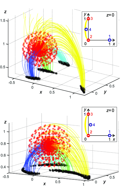
Figure 1.: Splitting of the magnetic-flux tubes originating from the energy-release region for the magnetic-source arrangement near the zone of topological instability (top panel) and away from this zone (bottom panel). Each red asterisk in the energy-release region is an initial point of the magnetic field line, which crosses the plane of emission $z\,{=}\,0.3$ (in the dimensionless units) at the respective black asterisk. The magnetic-field fluxes with different topological connectivity (i.e., terminating at different magnetic sources/sinks) are shown by different colors (yellow, green, blue, and cyan). The insets to the both panels show arrangement of the point-like magnetic sources with equal magnitudes—two positive (1 and 4) and two negative (2 and 3)—in the plane $z\,{=}\,0$. The yellow semilunar region in these insets is just the zone of topological instability.Fig1

The topological instability is realized, roughly speaking, when three magnetic sources with intermittent polarity are situated approximately along the same line, while the fourth source is located aside from them. In other words, they are arranged in the T-like configuration; for more details, see Figure 1 in our paper Dumin and Somov (2019) and the corresponding discussion there. In general, it is a very non-trivial fact that the number of the emissive spots is determined just by the zone of topological instability, because the concept of this instability was originally introduced by Gorbachev et al. (1988) in absolutely different context: it was associated with bifurcation and subsequent fast motion of a null point of the magnetic field, which might be responsible for the fast magnetic reconnection (e.g., Dumin and Somov, 2017). However, quite unexpectedly, the same bifurcation turned out to be also of crucial importance for splitting/merging of the projections of the magnetic fluxes. Of course, GKSS model is only one of possible options for the configuration of magnetic sources. However, by varying a single free parameter, it reproduces surprisingly well almost all typical structures of the AMF emissive ribbons.

A few natural questions arise now:

1. Can the same kinds of three- and four-ribbon AMFs be formed in the substantially different magnetic-source configurations (for example, with an unbalanced magnetic polarity)?

2. Is it possible to get more complex AMFs (namely, involving more than four ribbons) when a more sophisticated combination of the magnetic sources is realized?

As far as we know, such cases were not reported in the previous literature (apart from the “atypical” flares of much greater size); and it will be the aim of the subsequent section to represent the corresponding observations.

2 Observational Results

sec:Observ

To answer the above-posed questions, we performed a visual inspection of a large series of pictures of the emission in Ca II H line taken by the Solar Optical Telescope (SOT) onboard Hinode spacecraft (Kosugi et al., 2007; Tsuneta et al., 2008), which are stored in the Hinode archive, and confronted them with the corresponding magnetograms by the Helioseismic and Magnetic Imager (HMI) onboard SDO satellite (Pesnell, Thompson, and Chamberlin, 2012), which are available at the Joint Science Operations Center (JSOC) web-site. We sought for the AMFs, first of all, in the regions of the solar surface involving the complex configurations of the moderately-sized sunspots with intermittent polarity. Since they develop predominantly in the periods of high solar activity, we have analyzed in much detail, for example, the Hinode’s data for 2014. On the other hand, it was almost impossible to identify any AMFs in the years of low activity. There was no clear association of AMFs with the large-scale solar flares: sometimes they occurred in the vicinity of the powerful flares, while often beyond them. At last, since we analyzed only on-disk observations, attention was focused at the ribbons in the base of AMFs, while the corresponding chromospheric jets were not taken into consideration.

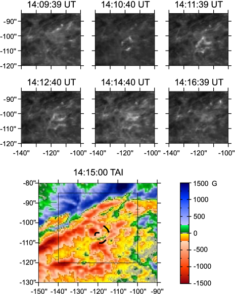
Figure 2.: Example of the three-ribbon AMF on 2 February 2014 that was formed by the unbalanced magnetic sources: a temporal sequence of the emission patterns in Ca II H line recorded by Hinode/SOT (top panels) vs. the pattern of magnetic fields obtained by SDO/HMI (bottom panel, courtesy of NASA/SDO and the HMI science team). A sketch of the ribbon configuration at 14:10:40 UT is plotted in the magnetogram.Fig2

As in the previous study, we preferred to use Ca II H line because it is emitted by a moderately heated plasma, ${\approx}10^{4}$ K. So, one can expect that the fine spatial features in the emission patterns are caused just by the geometric properties of the magnetic field lines rather than by the “physical” filamentation (such as development of the plasma instabilities, MHD waves, etc.).

Let us mention that the coordinate frame of Hinode/SOT experiences a substantial instability in the east–west direction. We did not try to compensate this instability but instead adjusted the magnetogram’s coordinates to the ones by Hinode/SOT. The color map in the magnetograms presented below looks rather unusual, it conforms with the recommendations of HMI team at the above-mentioned JSOC web-site (file HMI_M.ColorTable.pdf): the weak fields (within $\pm 24$ G) are shaded in gray, and the colors change sharply at $\pm 236$ G, when the magnetic field begin to affect the photospheric brightness (i.e., the sunspots are formed). Such color coding was designed to visually show the structure at both high and low field values. As follows from our experience, this color coding is really convenient.

2.1 AMF with Strongly Unbalanced Magnetic Fluxes

sec:AMF_unbal

The above-mentioned analysis enabled us to identify some interesting cases of the AMFs, unknown before. The first non-trivial situation, observed on 2 February 2014, is shown in Figure Fig2. Its emission patterns look like in the ordinary three-ribbon AMF: the ribbons quickly develop at the time scale about 1 min and then become diffuse and gradually decay in the subsequent few minutes. However, the corresponding magnetic sources are evidently unbalanced: The magnetogram demonstrates a complex cross-like arrangement of a few negative sources; but the positive sources exist only at very large distances, mostly in the northern part of the picture (while, according to the standard GKSS model, there must be at least one positive source in the vicinity of the ribbons). So, to explain such flares, GKSS model should be generalized to the case of unbalanced magnetic fluxes.

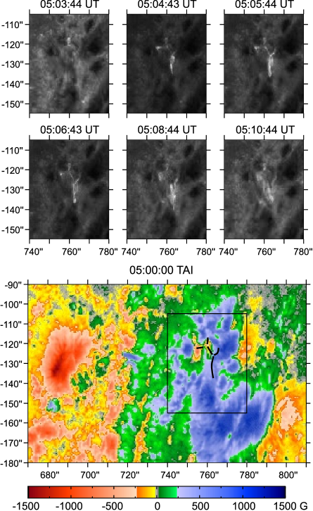
Figure 3.: Example of the five-ribbon flare in the solar chromosphere on 16 February 2014: a temporal sequence of the emission patterns in Ca II H line recorded by Hinode/SOT (top panels) vs. the map of magnetic fields obtained by SDO/HMI (bottom panel, courtesy of NASA/SDO and the HMI science team). A sketch of the ribbon configuration at 05:05:44 UT is plotted in the magnetogram.Fig3

2.2 AMF with Numerous Ribbons

sec:AMF_ribbons

The second—and most interesting—example of the unusual AMF is shown in Figure Fig3: this is a flare with a larger number of the emissive ribbons than in the previously-known three- and four-ribbon cases. It was recorded on 16 February 2014 approximately at 05 UT. As is seen, the flare begins to develop at 05:04:43 UT with three or four ribbons (depending on their definition). Then, at 05:05:44 and 05:06:43 UT one can see a complex structure composed of five (or even six) ribbons. At last, starting from 05:08:44 UT, the ribbons acquire a diffuse character and gradually disappear.

At the first glance, a semi-circular segment in the bottom right side of this structure looks like an arc extending into the upper layers of the atmosphere. However, one should keep in mind that this AMF occurred quite close to the west limb. Then, a projection of such an arc onto the picture plane would be bent to the limb, while just the opposite behavior is seen in the figure. So, we should conclude that the above-mentioned segment is located most probably on the surface.

A lifetime of the entire structure was 2–3 minutes, which is comparable to (or even somewhat less than) the lifetimes of ordinary AMFs reported before (e.g., Figure 2 in Shibata et al., 2007). On the other hand, a characteristic length of the entire structure in this case was about $20^{\prime\prime}$ (15 000 km), which is substantially greater than in the ordinary three- and four-ribbon AMFs ($3^{\prime\prime}{-}7^{\prime\prime}$, or 2000–5000 km). Besides, while thickness of the ribbons in the ordinary AMFs was $0.2^{\prime\prime}{-}0.4^{\prime\prime}$ (150–300 km), in our case they can be much thicker (up to $1^{\prime\prime}{-}2^{\prime\prime}$, or 700–1500 km); but this depends on the particular ribbon, and some of the ribbons remain thin.

To understand the structure of magnetic field responsible for this AMF, we superimposed a sketch of the emissive ribbons onto the magnetogram of the corresponding region (bottom panel in Figure Fig3). As is seen, the flare is produced by four magnetic sources (positive, negative, negative, and again positive) along the parallel and a few sources (mostly, positive) away from them, along the meridian. Such a configuration qualitatively reminds GKSS model of the magnetic field, where the topological instability with a complex flux splitting takes place, roughly speaking, at the T-like arrangement of the magnetic sources (see inserts in Figure Fig1); but this case evidently involves a larger number of the sources. A detailed topological analysis of such magnetic configurations is still to be done (for the recent reviews of topological models of the solar magnetic fields, see Longcope, 2005; Janvier, 2017). Besides, the total magnetic flux in the vicinity of AMF again seems to be substantially unbalanced, as in Figure Fig2.

In fact, the AMF presented in Figure Fig3 looks like a combination of two three-ribbon flares possessing one common ribbon. We observed also a few other cases when two three-ribbon structures were separated by a larger distance and did not have a common ribbon, but they appeared almost simultaneously (within 1–2 minutes). So, it is difficult to say if that was a single AMF or two different flares developing at the same time (in other words, if they were associated with one or two independent systems of the split magnetic fluxes and the corresponding energy-release regions)? It is interesting to mention that a “recurrent” (two-step) chromospheric microflare was observed also by Zeng et al. (2016), and the corresponding “steps” were separated by the time interval as long as 20 minutes.

In general, the multi-ribbon structures seen in Figures 5(a,b) from the above-cited work are very similar to AMFs. However, they were observed in the line He I 10 830 Å, which is sensitive to the higher temperatures than Ca II H. So, these images trace mostly the magnetic field lines themselves rather than their projections (ribbons) onto the denser layers.

3 Theoretical Interpretation

sec:Theory

It is a very nontrivial task to understand the geometric configuration of the reconnecting field lines in the unusual AMFs reported above. Really, a generic structure of the 3D null point, responsible for the magnetic reconnection, involves six asymptotic directions at ${\bf r}\to 0$ (where ${\bf r}=0$ is the null point), along which the magnetic field lines originate or disappear (Parnell et al., 1996; Dumin and Somov, 2016). Four of these asymptotes are “dominant”, so that the corresponding fluxes are concentrated and terminate at the magnetic sources of different polarity (two positive and two negative). Two other asymptotes are “recessive”, so that the respective field lines quickly deviate from them with increasing distance and scatter in space. Therefore, a standard pattern of the magnetic reconnection involves four fluxes; two of them being rooted in the positive sources, and two in negative.

So, if there are more than four fluxes in total or more than two fluxes of the same type, the standard picture is not applicable. Then, we should assume that (i) either there are more than one null point in the region of reconnection or (ii) the reconnection occurs in the high-order null point, where the number of incoming and outgoing fluxes can be greater (Zhugzhda, 1966; Lukashenko and Veselovsky, 2015; Lukashenko, 2016).

However, from the mathematical point of view, the case of the high-order null point is degenerate, and the probability of its realization tends to zero. So, the assumption of a few closely-located null points in the region of reconnection looks preferable. This point of view is especially supported by the recent data by Zeng et al. (2016), who clearly observed a “sequential branching” of the magnetic-flux tubes; see Figures 3(a) and 5(a,b) in the last-cited paper.

4 Conclusions

sec:Concl

1. The anemone microflares in the solar chromosphere represent a specific type of the transient phenomena, which are substantially different from the “atypical” multi-ribbon flares both from the viewpoint of their lifetime and the spatial scales. The AMFs, observed in the chromospheric lines, are not the “isolated” phenomena but manifest themselves also in EUV an X-rays, as was found recently by Zeng et al. (2016). Most probably, the complex multi-ribbon structure of AMFs is formed due to magnetic flux splitting at some height above the ribbons.

2. The GKSS model of magnetic field, utilized in our previous paper (Dumin and Somov, 2019), can give a rather good statistical description for the majority of three- and four-ribbon AMFs. However, as follows from the present work, it is possible to observe sometimes the more exotic flares, which are evidently beyond this model. These are, for example, the AMFs with more than four emissive ribbons as well as the flares occurring in the regions with strongly unbalanced magnetic polarity. Most probably, such flares involve a few null points in the region of reconnection, resulting in the sequential branching of the magnetic fluxes. However, the detailed topological models of these events still need to be developed.

Acknowledgments

YVD is grateful to A.V. Getling, A.V. Oreshina, and I.V. Oreshina for consultations on the processing of magnetic fields, A.T. Lukashenko for the discussion of the high-order null points, as well as to G.G. Motorina and A.V. Stepanov for valuable comments and suggestions.

Hinode is a Japanese mission developed and launched by ISAS/JAXA, with NAOJ as domestic partner and NASA and STFC (UK) as international partners. It is operated by these agencies in co-operation with ESA and NSC (Norway).

Declaration of Potential Conflicts of Interest  The authors declare that they have no conflict of interest.

References

- Asai et al. (2009) Asai, A., Shibata, K., Ishii, T.T., et al.: 2009, Evolution of the Anemone AR NOAA 10798 and the Related Geo-effective Flares and CMEs. J. Geophys. Res. 114, A00A21.
- Brown and Priest (1999) Brown, D.S., Priest, E.R.: 1999, The Topological Behaviour of Stable Magnetic Separators. Sol. Phys. 190, 25.
- Christe et al. (2008) Christe, S., Hannah, I.G., Krucker, S., McTiernan, J., P., L.R.: 2008, RHESSI Microflare Statistics. I. Flare-finding and Frequency Distributions. ApJ 677, 1385.
- Curdt and Tian (2011) Curdt, W., Tian, H.: 2011, Spectroscopic Evidence for Helicity in Explosive Events. A&A 532, L9.
- Dalmasse et al. (2015) Dalmasse, K., Chandra, R., Schmieder, B., Aulanier, G.: 2015, Can we Explain Atypical Solar Flares? A&A 574, A37.
- Dumin and Somov (2016) Dumin, Y.V., Somov, B.V.: 2016, On the Most Typical Structure of Three-dimensional Magnetic Reconnection. Astron. Lett. 42, 774.
- Dumin and Somov (2017) Dumin, Y.V., Somov, B.V.: 2017, Observation of “Topological” Microflares in the Solar Atmosphere. Res. Notes AAS 1, 15.
- Dumin and Somov (2019) Dumin, Y.V., Somov, B.V.: 2019, Topological Model of the Anemone Microflares in the Solar Chromosphere. A&A 623, L4.
- Gorbachev and Somov (1988) Gorbachev, V.S., Somov, B.V.: 1988, Photospheric Vortex Flows as a Cause for Two-Ribbon Flares: A Topological Model. Sol. Phys. 117, 77.
- Gorbachev et al. (1988) Gorbachev, V.S., Kel’ner, S.R., Somov, B.V., Shvarts, A.S.: 1988, A New Topological Approach to the Question of the Trigger for Solar Flares. Soviet Ast. 32, 308.
- Hannah et al. (2008) Hannah, I.G., Christe, S., Krucker, S., Hurford, G.J., Hudson, H.S., Lin, R.P.: 2008, RHESSI Microflare Statistics. II. X-Ray Imaging, Spectroscopy, and Energy Distributions. ApJ 677, 704.
- Harrison (1997) Harrison, R.A.: 1997, EUV Blinkers: The Significance of Variations in the Extreme Ultraviolet Quiet Sun. Sol. Phys. 175, 467.
- Inverarity and Priest (1999) Inverarity, G.W., Priest, E.R.: 1999, Magnetic Null Points due to Multiple Sources of Solar Photospheric Flux. Sol. Phys. 186, 99.
- Janvier (2017) Janvier, M.: 2017, Three-dimensional Magnetic Reconnection and Its Application to Solar Flares. J. Plas. Phys. 83, 535830101.
- Kosugi et al. (2007) Kosugi, T., Matsuzaki, K., Sakao, T., et al.: 2007, The Hinode (Solar-B) Mission: An Overview. Sol. Phys. 243, 3.
- Longcope (2005) Longcope, D.W.: 2005, Topological Methods for the Analysis of Solar Magnetic Fields. Liv. Rev. Sol. Phys. 2, 7.
- Lukashenko (2016) Lukashenko, A.T.: 2016, Description of a Potential Vector Field Without Sources Near Null Points of Higher Orders in 3D Space. Moscow Univ. Math. Bull. 71, 146.
- Lukashenko and Veselovsky (2015) Lukashenko, A.T., Veselovsky, I.S.: 2015, General Principles of Describing Second and Higher Order Null Points of a Potential Magnetic Field in 3D. Geomag. Aeron. 55, 1152.
- Nishizuka et al. (2011) Nishizuka, N., Nakamura, T., Kawate, T., Singh, K.A.P., Shibata, K.: 2011, Statistical Study of Chromospheric Anemone Jets Observed with Hinode/SOT. ApJ 731, 43.
- Parnell et al. (1996) Parnell, C.E., Smith, J.M., Neukirch, T., Priest, E.R.: 1996, The Structure of Three-dimensional Magnetic Neutral Points. Phys. Plas. 3, 759.
- Pesnell, Thompson, and Chamberlin (2012) Pesnell, W.D., Thompson, B.J., Chamberlin, P.C.: 2012, The Solar Dynamics Observatory (SDO). Sol. Phys. 275, 3.
- Shibata et al. (2007) Shibata, K., Nakamura, T., Matsumoto, T., Otsuji, K., Okamoto, T.J., Nishizuka, N., et al.: 2007, Chromospheric Anemone Jets as Evidence of Ubiquitous Reconnection. Science 318, 1591.
- Singh et al. (2011) Singh, K.A.P., Shibata, K., Nishizuka, N., Isobe, H.: 2011, Chromospheric Anemone Jets and Magnetic Reconnection in Partially Ionized Solar Atmosphere. Phys. Plas. 18, 111210.
- Singh et al. (2012) Singh, K.A.P., Isobe, H., Nishizuka, N., Nishida, K., Shibata, K.: 2012, Multiple Plasma Ejections and Intermittent Nature of Magnetic Reconnection in Solar Chromospheric Anemone Jets. ApJ 759, 33.
- Somov (2013) Somov, B.V.: 2013, Plasma Astrophysics, Part II: Reconnection and Flares, 2nd edn. Springer, NY.
- Tsuneta et al. (2008) Tsuneta, S., Suematsu, Y., Ichimoto, K., et al.: 2008, The Solar Optical Telescope for the Hinode Mission: An Overview. Sol. Phys. 249, 167.
- Wang et al. (2014) Wang, H., Liu, C., Deng, N., et al.: 2014, Study of Two Successive Three-Ribbon Solar Flares on 2012 July 6. ApJ 781, L23.
- Zeng et al. (2016) Zeng, Z., Chen, B., Ji, H., Goode, P.R., Cao, W.: 2016, Resolving the Fan-Spine Reconnection Geometry of a Small-Scale Chromospheric Jet Event with the New Solar Telescope. ApJ 819, L3.
- Zhugzhda (1966) Zhugzhda, Y.D.: 1966, The Neutral (Null) Points of Magnetic Fields. Geomagnetism i Aeronomiya 6, 506. in Russian.