DeepMoD: Deep learning for Model Discovery in noisy data

Abstract

We introduce DeepMoD, a Deep learning based Model Discovery algorithm. DeepMoD discovers the partial differential equation underlying a spatio-temporal data set using sparse regression on a library of possible functions and their derivatives. A neural network is used as function approximator and its output is used to constructs the function library, allowing to perform the sparse regression within the neural network. This construction makes it extremely robust to noise, applicable to small data sets, and, contrary to other deep learning methods, does not require a training set. We benchmark our approach on several physical problems such as the Burgers’, Korteweg-de Vries and Keller-Segel equations, and find that it requires as few as $\mathcal{O}(10^{2})$ samples and works at noise levels up to $75\%$. Motivated by these results, we apply DeepMoD directly on noisy experimental time-series data from a gel electrophoresis experiment and find that it discovers the advection-diffusion equation describing this system.

Keywords Model discovery  $\cdot$ Deep learning  $\cdot$ Sparse regression

1 Introduction

Recently, efforts have been made to combine data-driven science with bottom up physical modelling in a new field known as "theory-guided data science" (1). Integrating first-principle models with data science has already proven successful in material science (2), earth science (3, 4, 5, 6) and fluid mechanics (7, 8). This approach has proven useful to infer coefficients of known PDEs from artificial data, the so called Physics-Informed Neural Networks (PINNs) (9, 10, 11, 12), and even to directly discover physical models from artificial data, i.e., PDE-NET (13, 14), PDE-Stride (15) and PDE-Find (16, 17).

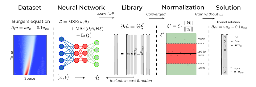
Figure 1: Work-flow of the algorithm: the neural network takes the coordinates of the problem as input and approximates the noisy dataset as output. From this output, the library of candidate terms is constructed and subsequently included in the regression part of cost function of the network, which consists of the MSE-loss, a regression loss and an $L_{1}$ regularization. Once the neural network has converged or reached the maximal numbers of allowed iterations, the elements of $\vec{\xi}$ are normalized and thresholded. The resulting sparsity pattern is then used to train the network one final time without $L_{1}$ penalty to find the unbiased coefficients.

The problem of data-driven model discovery of PDEs has been approached from several different directions. While information theory provides a rigorous basis for model selection, it becomes computationally infeasible to compare the information criteria of a vast amount of candidate models (18). Alternatively, an approach to discover a PDE from a spatio-temporal data-set is to use sparse regression model selection schemes such as PDE-FIND as proposed by (16, 17). In this approach, the PDE underlying a dataset $u(\{x,t\})$ is discovered by writing the model discovery task as a regression problem,

$$\partial_{t}u=\Theta\xi,$$ (1)

where $\Theta$ is a matrix containing a library of polynomial and spatial derivative functions (e.g. $u,u_{x},uu_{x}$). Here model discovery turns into finding a sparse representation of the coefficient vector $\xi$. Rudy et al. (16) introduce the regression algorithm TrainSTridge to solve this task on artificial data such as the Burgers’ equation in hydrodynamics, the Schrödinger equation in quantum mechanics and the Kuramoto-Sivashinsky equation in chaos theory (16). Although very promising, this method is sensitive to noise and requires a large number of samples. This can largely be traced back to errors in the numerical differentiation and hence inaccurate derivatives in the library $\Theta$. These traits essentially render the method unfeasible on noisy experimental data. To overcome this, we propose to use automatic differentiation within the neural network to accurate calculate the derivatives in the library function. Indeed, Rudy et al. (16) recognize this possibility to improve the performance of exisiting model discovery methods such as SINDY (18) and PDE-find (16). A first approach would be to use a neural network to learn the mapping of the data, i.e. $\{x,t\}\to u$, and then employ automatic differentiation to accurately calculate the derivatives of $u$ with respect to $x$ and $t$, which can then be used to construct $\Theta$. Unfortunately, this implementation is susceptible to overfitting noisy data, which significantly decreases the accuracy of the library.

The novelty of our work is that we circumvent this ubiquitous issue by implementing Eq. 1 within the cost function of the neural network. Consequently, training the network not only adjusts the weights and biases of the network, but also adjusts the components of the sparse vector $\xi$, corresponding to Eq. 1. An $L_{1}$ term on $\xi$ is added to the cost function to ensure its sparsity. Training the neural network yields the underlying PDE and denoises the data set. We show that this approach outperforms state-of-the-art methods of model selection (16, 12) by applying it on artificial data sets of the Burgers’, Korteweg-de Vries (KdV), 2D advection diffusion and the Keller-Segel equations (See SI for a comparison). Finally we demonstrate that DeepMoD can discover the PDE underlying an electrophoresis experiments and discover the 2D advection diffusion equation. This shows that this deep learning based selection algorithm can consistently discover the second order advection diffusion equation directly from a simple time-series of images of a diffusing dye.

Methods

Our goal is to develop a fully-automated procedure which discovers the partial differential equation (PDE) underlying a measured data set. Given a data set $u(\{x,t\})$, we can write this problem as,

$$\partial_{t}u(x,t)=\mathcal{F}\left(u,u_{x},uu_{x},u_{xx},...\right),$$ (2)

where we seek the function $\mathcal{F}$. To find $\mathcal{F}$, we generate a large set of possible models by considering all permutations of a library of candidate terms. The choice of the library depends on the problem at hand but generally consists of polynomial basis functions and their corresponding spatial derivatives. For example, in the one dimensional examples we present in this paper, the library consists of all polynomials in $u$ up to second order, the derivatives of $u$ with respect to the coordinates (e.g. $\partial_{x}u$) up to third order and any possible combinations of these two sets (e.g. $u^{2}u_{xx}$), totalling just 12 terms. However, one can construct more than 4000 unique models from this limited set of functions, rendering an information theory approach computationally unfeasible (18).

We circumvent this problem by utilizing a sparse regression approach, in which the model discovery problem is rewritten as

$$\partial_{t}u=\Theta\xi,$$ (3)

where $\partial_{t}u$ is a column vector of size $N$ containing the time derivative of each sample and $\Theta$ contains all $M$ possible terms for each of the samples, so that we can write it as

$${\Theta=\begin{bmatrix}1&u(\{x,t\}_{0})&u_{x}(\{x,t\}_{0})&\dots&u^{2}u_{xx}(\{x,t\}_{0})\\ 1&u(\{x,t\}_{1})&u_{x}(\{x,t\}_{1})&\dots&u^{2}u_{xx}(\{x,t\}_{1})\\ \vdots&\vdots&\vdots&\ddots&\vdots\\ 1&u(\{x,t\}_{N})&u_{x}(\{x,t\}_{N})&\dots&u^{2}u_{xx}(\{x,t\}_{N})\\ \end{bmatrix}}$$ (4)

Since $\Theta$ contains significantly more terms than required, most coefficients in $\xi$ will be zero and hence we are looking for a sparse solution of the vector $\xi$. Note that since we directly discover the governing PDE rather than a closed form of the solution, the differential equation that we discover is independent of the precise boundary conditions of the problem at hand. In the next section, we discuss how this regression task is solved using Lasso, a sparsity promoting regression method, within a neural network.

Lasso in neural network

In order to solve the regression task of the previous section we need to contruct the function library, $\Theta$. Here we employ a densely-connected feed-forward neural network which takes the spatial and temporal coordinates of the problem, i.e. $\{x,t\}$ as input, and outputs $\hat{u}$, an approximation of $u$ at $\{x,t\}$ (9, 10). In other words, the neural network approximates the function $u(x,t)$ and employs this approximation to construct the library function, $\Theta$. Using feed-forward neural networks as function approximators has three major advantages, i) they naturally accommodate non-linear constraints, without the need to linearize any operators, ii) they do not require any time-stepping scheme and iii) they allow the use of automatic differentiation to accurately differentiate the output of the neural network with respect to the input coordinates.

The neural network we consider here is trained by optimizing the cost function,

$$\mathcal{L}=\mathcal{L}_{MSE}+\mathcal{L}_{Reg}+\mathcal{L}_{L_{1}}.$$ (5)

Here, $\mathcal{L}_{MSE}$, is the mean squared error (MSE) of the output of the neural network $\hat{u}$ with respect to the dataset $u(\{x,t\})$,

$$\mathcal{L}_{MSE}=\frac{1}{N}\sum_{i=1}^{N}|u(\{x,t\}_{i})-\hat{u}_{i}|^{2}.$$ (6)

The last two terms of Eq. 5 correspond to the Lasso regularization: $\mathcal{L}_{Reg}$ performs regression to find the coefficient vector $\xi$ and $\mathcal{L}_{L_{1}}$ is an $L_{1}$ regularizer on $\xi$. In order to implement the regression problem (Eq. 3) within the neural network, we introduce the regression based cost function,

$$\mathcal{L}_{Reg}=\frac{1}{N}\sum_{i=1}^{N}|\Theta_{ij}\xi_{j}-\partial_{t}\hat{u}_{i}|^{2}.$$ (7)

Note that the coefficient vector $\xi$ is updated alongside the weights and biases of the neural network, while the terms in $\Theta$ are computed from the output of the neural network (i.e. $\hat{u}$). Automatic differentiation is used to calculate all the spatial and temporal derivatives in $\Theta$, returning machine-precision derivatives. This approach is considerably more accurate than any form of numerical differentiation. Moreover, $\mathcal{L}_{Reg}$ acts as a regularizer on $\hat{u}$, preventing overfitting of the noisy data set, even though our library contains a large amount of terms (See Results and Fig. 2c).

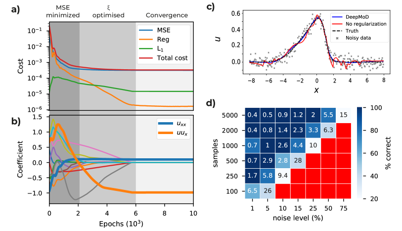
Figure 2: (a) Cost functions and (b) coefficient values, $\xi$, as function of the number of epochs for the Burgers’ dataset consisting of 2000 points and $10\%$ white noise. Initially, the neural network optimizes the MSE and only after the MSE is converged the coefficient vector is optimized by the network. (c) Velocity field $u$ for $t=5$ obtained after training with (no overfitting) and without (overfitting) the regression regularization $\mathcal{L}_{Reg}$. (d) The values in the grid indicate the accuracy of the algorithm tested on the Burgers’ equation, defined as the mean relative error over the coefficients, as function of the sample size of the data set and level of noise. The coloring represents the fraction of correct runs (Red indicates that in none of the five iterations the correct PDE is discovered).

Finally, an $L_{1}$ regularization on the vector $\xi$ is added to ensure its sparsity,

$$\mathcal{L}_{L_{1}}=\lambda\sum_{i=2}^{M}|\xi^{i}|.$$ (8)

Here $\lambda$ is a constant setting the strength of the regularization (further discussed in the SI).

The total cost of the neural network is then minimized using the Adam optimizer. The combination of the MSE term and the regression term in the cost function constrain the network in such a way that it converges to the right solution. To determine if the network has converged, we introduce a convergence criterion. As we show in Fig. 2(a,b), the MSE converges before $\xi$ does, so that our criterion is based on the convergence of $\xi$:

$$\text{max}\left(\frac{\partial\mathcal{L}}{\partial\xi_{i}}\frac{||\partial_{t}u||}{||\Theta_{i}||}\right)<\rm{tol}.$$ (9)

This criterion states that the maximum value of the gradient of the loss function with respect to the coefficients must be smaller than a given tolerance. Note here that we have scaled the gradients as we discuss in the next paragraph. Since it is not guaranteed the network will reach this tolerance, we train the network until the convergence criterion is satisfied, or for a maximum amount of iterations.

Normalization and thresholding

When the neural network has finished training, we obtain the sparse vector $\xi$. Despite the $L_{1}$ regularization, most terms will be non-zero and hence we need to threshold the small coefficients to obtain the true sparse representation. Since each term has different dimensions, Eq. 2 is rendered dimensionless,

$$\partial_{t}u\to\frac{\partial_{t}u}{||\partial_{t}u||},\Theta\to\frac{\Theta}{||\Theta||},\xi\to\xi\frac{||\Theta||}{||\partial_{t}u||},$$ (10)

where $||\Theta||$ is the norm of each column of $\Theta$ and $||\partial_{t}u||$ the norm of the time-derivative vector. As a result of this transformation, components of $\xi$ will typically be $\mathcal{O}(1)$.

Thresholding prunes components with a negligible impact on the data set by setting all their values to zero. Figure 3 shows the distribution of the scaled coefficients before thresholding for the $1\%$, $10\%$ and $25\%$ noise runs with sample sizes of $2000$ and $5000$ (corresponding to the data in figure 2D). Figure 3 shows that the required terms (i.e. $u_{xx}$ and $uu_{x}$) considerably stand out relative to the others. We show that up to moderate noise levels $<20\%$ (Fig. a and b) the exact value of the threshold does not significantly impacts which terms are eventually pruned. The difference between the largest non-featuring and smallest featuring terms is typically up to an order of magnitude. For very high noise levels $>20\%$ levels (See Fig. 3 c) the accuracy of the pruning is much more sensitive to the exact value and more advanced sparsity algorithms could be required to obtain more robust model selection (See Discussion).

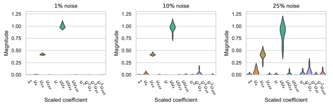
Figure 3: Scaled coefficients before thresholding for the Burgers equation with $1\%$ noise (a), $10\%$ noise (b) and $25\%$ (c). This indicates that there is a considerable difference between the terms that do and do not feature in the PDE.

We then train the network one final time without $L_{1}$ penalty and with the regression term only containing the terms selected in the first cycle, to find an unbiased estimate of the coefficients of the underlying PDE.

Results

We test the performance of DeepMoD on a set of case studies: the Burgers’ equation with and without shock, the Korteweg - de Vries equation, the 2D advection-diffusion equation and the Keller-Segel model for chemotaxis. These examples show the ability of DeepMoD to handle (1) non-linear equations, (2) solutions containing a shock wave, (3) coupled PDEs and finally (4) higher dimensional and experimental data.

Non-linear PDEs

We apply DeepMoD to recover various non-linear and higher order differential equations. As examples we consider Burgers’ equation (in the SI we the Korteweg-de Vries equation, which contains a third-order derivative). The Burgers’ equation occurs in various areas of gas dynamics, fluid mechanics and applied mathematics and is evoked as a prime example to benchmark model discovery (16, 14) and coefficient inference algorithms (9, 10, 12), as it contains a non-linear term as well as second order spatial derivative,

$$\partial_{t}u=-uu_{x}+\nu u_{xx}.$$ (11)

Here $\nu$ is the viscosity of the fluid and $u$ its velocity field. We use the dataset produced by Rudy et al. (16), where $\nu=0.1$. The numerical simulations for the synthetic data were performed on a dense grid for numerical accuracy. DeepMoD requires significantly less datapoints than this grid and we hence construct a smaller dataset for DeepMoD by randomly sampling the results through space and time. From now on, we will refer to randomly sampling from this dense grid simply as sampling. Also note that this shows that our method does not require the data to be regularly spaced or stationary in time. For the data in Fig. 2 we add $10\%$ white noise and sampled 2000 points for DeepMoD to be trained on.

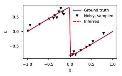
Figure 4: Ground truth, Noisy and Inferred data at $t=0.8$ for the Burgers’ equation with a shock wave (10$\%$ noise and 2000 sample points).

We train the neural network using an Adam optimizer (see SI for details) and plot the different contributions of the cost function as a function of the training epoch in Fig. 2a and we show the value of each component of $\xi$ as a function of the training epoch in Fig. 2b. Note that for this example, after approximately 2000 epochs, the MSE is converged, while at the same time we observe the components of $\xi$ only start to converge after this point. We can thus identify three ’regimes’: in the initial regime (0 - 2000 epochs), the MSE is trained. Since the output of the neural network is far from the real solution, so is $\Theta$, and the regression task cannot converge (See first 2000 epochs in Fig. 2b). After the MSE has converged, $\hat{u}$ is sufficiently accurate to perform the regression task and $\xi$ starts to converge. After this second regime (2000 - 6000 epochs), all components of the cost converged ($>$6000 epochs) and we can determine the solution. From this, we obtain a reconstructed solution (see Fig. 2b) and at the same time recover the underlying PDE, with coefficients as little as $1\%$ error in the obtained coefficients. We show the impact of including the regression term in the cost function in Fig.2c, where the obtained solution of DeepMoD is compared with a neural network, solely trained on the MSE, to reconstruct the data. Including the regression term regularizes the network and prevents overfitting, despite the many terms in the library. We conclude that it is the inclusion of the regression in the neural network which makes DeepMoD robust to noisy data and prevents overfitting.

Next, we characterize the robustness of DeepMoD in Fig. 2d, where we run DeepMod for five times (differently sampled data set) for a range of sample sizes and noise levels. The color in Fig. 2d shows how many of the five runs return the correct equation and the value in the grid displays the mean error over all correct runs. Observe that at vanishing noise levels, we recover Eq. 11 with as little as 100 data-points, while for 5000 data points we recover the PDE with noise levels of up to $75\%$. Between the domain where we recover the correct equation for all five runs and the domain where we do not recover a single correct equation, we observe an intermediate domain where only a fraction of the runs return the correct equation, indicating the importance of sampling (See SI 2 for further discussion).

To benchmark DeepMoD, we can directly compared the performance of our algorithm with respect to two state of the art methods, (i): PDE-Find by Rudy et al. (16) and (ii) PDE-Stride by Maddu et al. (15). We considered an identical Burgers’ data set and for $10^{5}$ data points, approach (i) recovers the correct equation for up to $1\%$ Gaussian noise (16) while method (ii) discovers the correct equation up to $5\%$ noise (15). Compared to the results in Fig. 2d we note that even for two order of magnitude fewer samples points, $10^{3}$ w.r.t. $10^{5}$, DeepMoD recovers the correct equation up to noise levels $>50\%$ Gaussian noise. DeepMoD allows up to two orders of magnitude higher noise-levels and smaller sample sizes with respect to state-of-the-art model discovery algorithms. The reason DeepMoD is considerable more robust w.r.t. noise and sample size is two-fold: (i) numerical differentiation or denoising requires a relatively fine sampling grid to accurately aproximate the derivatives present in the library function. (ii) Since the functions in the library of the neural network are calculated with respect to the inferred solution, our approach is considerably less sensitive to elevated noise levels (See Fig. 2c). We show in the SI that DeepMod has similar performance for the KdV equation, which contains a third order spatial derivative.

Shock wave solutions

If the viscosity is too low, the Burgers’ equation develops a discontinuity called a shock (See Fig. 4). Shocks are numerically hard to handle due to divergences in the numerical derivatives. Since DeepMoD uses automatic differentiation we circumvent this issue. We adapt the data from Raissi et al (10), which has $\nu=0.01/\pi$, sampling 2000 points and adding 10 $\%$ white noise (See Fig. 4). We recover ground truth solution of the Burgers’ equation as well as the corresponding PDE,

$$\partial_{t}u=-0.99uu_{x}+0.0035u_{xx},$$ (12)

with a relative error of 5$\%$ on the coefficients. In Fig. 4 we show the inferred solution for $t=0.8$.

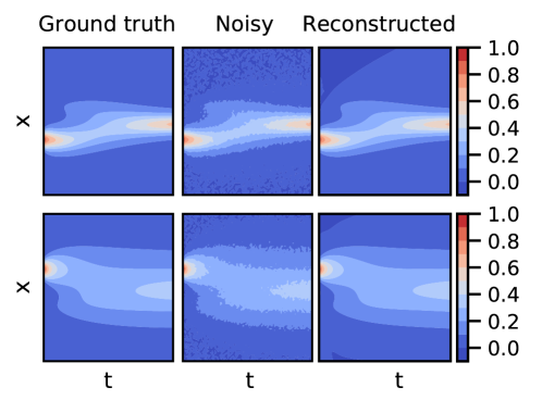
Figure 5: Ground truth, noisy and reconstructed solutions for the density of cells, $u$ (top row) and the density of secreted chemicals $w$ (bottom row) in the Keller Segel model for 5 $\%$ white noise and 10000 samples.

Coupled differential equations

Next, we apply DeepMod to a set of coupled PDE’s in the form of the Keller-Segel (KS) equations, a classical model for chemotaxis (19, 20). Chemotactic attraction is one of the leading mechanisms that accounts for the morphogenesis and self-organization of biological systems. The KS model describes the evolution of the density of cells $u$ and the secreted chemical $w$,

$$\begin{split}\partial_{t}u=\nabla\cdot\left(D_{u}\nabla u-\chi u\nabla w\right)\\ \partial_{t}w=D_{w}\Delta w-kw+hu.\end{split}$$ (13)

Here the first equation represents the drift-diffusion equation with a diffusion coefficient of the cells, $D_{u}$ and a chemotactic sensitivity $\chi$, which is a measure for the strength of their sensitivity to the gradient of the secreted chemical $w$. The second equation represents the reaction diffusion equation of the secreted chemical $w$, produced by the cells at a rate $h$ and degraded with a rate $k$. For a 1D system, we sample 10000 points of $u$ and $w$ for parameter values of $D_{u}=0.5$, $D_{v}=0.5$, $\chi=10.0$, $k=0.05$ and $h=0.1$ and add 5 $\%$ white noise. We choose a library consisting of all spatial derivatives (including cross terms) as well as first order polynomial terms, totalling 36 terms. For these conditions we recover the correct set of PDEs,

$$\begin{split}\partial_{t}u=0.50u_{xx}-9.99uw_{xx}-10.02u_{x}w_{x}\\ \partial_{t}w=0.48w_{xx}-0.049w+0.098u,\end{split}$$ (14)

as well as the reconstructed fields for $u$ and $w$ (See Fig. 5). Note that even the coupled term, $u_{x}w_{x}$ , which becomes vanishingly small over most of the domain, is correctly identified by the algorithm, even in the presence of considerable noise levels.

Experimental data

To showcase the robustness of DeepMoD on high-dimensional and experimental input data, we consider a 2D advection diffusion process described by,

$$\partial_{t}u=-\nabla\cdot\left(-D\nabla u+\vec{v}\cdot u\right),$$ (15)

where $\vec{v}$ is the velocity vector describing the advection and $D$ is the diffusion coefficient. In the SI we apply DeepMod on a simulated data-set of Eq. 15, with as initial condition, a 2D Gaussian with $D=0.5$ and $\vec{v}=(0.25,0.5)$. For as little as 5000 randomly sampled points we recover the correct form of the PDE as well as the vector $\vec{v}$ for noise levels up to $\approx 25\%$. In the absence of noise the correct equation is recovered with as little as 200 sample points through space and time (See SI 2). This number is surprisingly small considering this is an 2D equation.

Finally, we apply DeepMoD on a time-series of images from an electrophoresis experiment, tracking the advection-diffusion of a charged purple loading dye under the influence of a spatially uniform electric field (See SI for further details). In Fig. 6a we show time-lapse images of the experimental setup where we measure the time-evolution of two initial localised purple dyes. Fig. 6b shows the resultant 2D density field for three separate time-frames (in arbitrary units), corresponding to the red square in Fig. 6a by substracting the reference image (no dye present). The dye displays a diffusive and advective motion with constant velocity $v$, which is related to the strength of the applied electric field.

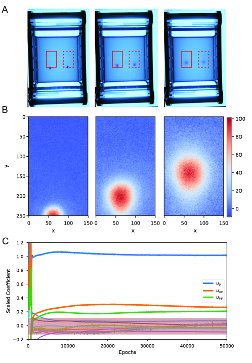
Figure 6: (a) Time-serie images of the electrophoresis essay. The two red boxes indicate the analysed region. (b) Region indicated in the solid red box of (a) showing the density of the dye at three different time-frames (in pixels). (c) Scaled coefficients values of all the candidate for a single run. The pink region indicates the terms with scaled coefficient $|\xi|<0.1$.

We apply DeepMoD on 5000 sampled data-points sampled through space and time and consistently recover the advection term $u_{y}$ as well as the two diffusive components ($u_{xx}$ and $u_{yy}$). In Fig. 6c we show the scaled coefficients as function of the number of epochs. After thresholding the scaled coefficients ($|\xi|<0.1$), we obtain for thre unscaled coefficients, the resultant advection diffusion equation,

$$0.31u_{y}+0.011u_{xx}+0.009u_{yy}=0.$$ (16)

Analysing the second diffusing dye (dashed box in Fig. 6) result in nearly identical values for the drift velocity, $v\approx 0.3$, and the diffusion coefficients, $D\approx 0.01$ (See SI) indicating the robustness of the obtained value of $D$ and $v$. In contrast to the artificial data presented in previous paragraphs, some higher-order non-linear terms, in particular $uu_{yy}$ and $uu_{xx}$ remain small, yet non-zero. This suggests that an automatic threshold strategy may not guarantee the desired sparse solution. Fixing a threshold of the scaled coefficients ($|\xi|<0.1$ in this particular case) or other thresholding strategies such as coefficient cluster detection would be better suited for this task.

Discussion

In this paper we presented DeepMoD, a novel model-discovery algorithm, utilising neural networks to discover the underlying PDE of a spatio-temporal dataset. We demonstrate the algorithm on 5 artificially obtained case studies: Burgers’ (with/without shock), Korteweg-de Vries, advection diffusion and Keller-Segel equations as well as on an experimental data-set of the advection diffusion equation. In contrast to many of the state of the art model discovery algorithms DeepMoD is very robust with respect to elevated noise levels and resilient to small data set sizes, demonstrating an automated model selection task directly from an experimental obtained time-series measurement. DeepMoD allows higher dimensional input/output as well as coupled PDEs as demonstrated with the 2D advection diffusion and Keller-Segel equation.

Through the use of automatic differentiation, combined with a regression-based regularization, the approximation of the spatio-temporal derivatives in noisy data is strongly enhanced. DeepMoD combines two previously established ideas, (i) a regression-based approach to model discovery (pioneered by e.g. Rudy et al. (16, 17)) and (ii) the ability of neural networks to infer system parameters in the context of Physics Informed Neural Networks (Raissi et al. (9, 10, 12). We show that combining both approaches strongly improves the model discovery task at hand and results in an increased robustness with respect to noise-levels and sample size for model discovery tasks. This approach, for the first time, allows model selections on highly noisy and hence low spatial/temporal resolution experimental data, which to date is one of the prime challenges of this field. DeepMoD also allows to infer the various type of diffusive, chemo-tactic equations, from single particle tracking (SPT) data by following a similar approach as (16), which will advance existing approaches to infer potentially anomalous diffusive processes from SPT data (21, 22).

The success of this approach however strongly relies on (i) the completeness of the library functions in $\Theta$ and (ii) a threshold of small yet non-zero terms. (i) If the underlying functions are not present in the library, DeepMoD will not return the correct underlying equation. This problem however can be identified via a cross-validation procedure on a set on a spatial/temporal domain that is not present in the training data. If correct, the resultant equation should perform well outside the spatio-temporal domain of training. Conversely, since we use neural networks as function approximator, the function library, $\Theta$, can be tailored to the problem at hand and thus contain non-linear functions of the network’s output, e.g. $\sin u$, $1/(1+u)$. This can be used to model the spatio-temporal evolution of e.g. genetic activation networks (23). We have empirically found that including these extensive libraries does not result in over-fitting the sparse coefficient vector of the data, even though the optimisation contains more degrees of freedom. (ii) While the threshold criterion based on the standard deviation of the coefficient vector provides consistent results throughout the artificial data-sets, this approach understandably fails when either the data is very noisy or when experimental artefacts introduce non-zero contributions of higher order terms. While we have shown in Fig. 3 that up to moderate noise levels the exact value of the threshold does not impact the results significantly, for very high noise levels more advanced sparsity selections algorithms like PDE-find (16) or coefficient clustering schemes would be more appropriate.

Besides the model selection capabilities, DeepMoD demonstrates its usefulness to denoise data and allows accurately approximating derivatives from noisy data, a notoriously difficult task to solve with classical interpolation and finite difference schemes. Employing this "function library based" regulation of neural network architecture may boost the enhancement of e.g. super resolution images through physics informed regularisation (24, 25).

References

- Karpatne et al. (2017a) Anuj Karpatne, Gowtham Atluri, James H Faghmous, Michael Steinbach, Arindam Banerjee, Auroop Ganguly, Shashi Shekhar, Nagiza Samatova, and Vipin Kumar. Theory-guided data science: A new paradigm for scientific discovery from data. IEEE Transactions on Knowledge and Data Engineering, 29(10):2318–2331, 2017a.
- Wagner and Rondinelli (2016) Nicholas Wagner and James M Rondinelli. Theory-guided machine learning in materials science. Frontiers in Materials, 3:28, 2016.
- Karpatne et al. (2017b) Anuj Karpatne, William Watkins, Jordan Read, and Vipin Kumar. Physics-guided neural networks (pgnn): An application in lake temperature modeling. arXiv preprint arXiv:1710.11431, 2017b.
- Reichstein et al. (2019) Markus Reichstein, Gustau Camps-Valls, Bjorn Stevens, Martin Jung, Joachim Denzler, Nuno Carvalhais, et al. Deep learning and process understanding for data-driven earth system science. Nature, 566(7743):195, 2019.
- Kong et al. (2018) Qingkai Kong, Daniel T Trugman, Zachary E Ross, Michael J Bianco, Brendan J Meade, and Peter Gerstoft. Machine learning in seismology: Turning data into insights. Seismological Research Letters, 90(1):3–14, 2018.
- de Bezenac et al. (2017) Emmanuel de Bezenac, Arthur Pajot, and Patrick Gallinari. Deep learning for physical processes: Incorporating prior scientific knowledge. arXiv preprint arXiv:1711.07970, 2017.
- Maulik and San (2017) Romit Maulik and Omer San. A neural network approach for the blind deconvolution of turbulent flows. Journal of Fluid Mechanics, 831:151–181, 2017.
- Miyanawala and Jaiman (2017) Tharindu P Miyanawala and Rajeev K Jaiman. An efficient deep learning technique for the navier-stokes equations: Application to unsteady wake flow dynamics. arXiv preprint arXiv:1710.09099, 2017.
- Raissi et al. (2017a) Maziar Raissi, Paris Perdikaris, and George Em Karniadakis. Physics informed deep learning (part ii): data-driven discovery of nonlinear partial differential equations. arXiv preprint arXiv:1711.10566, 2017a.
- Raissi et al. (2017b) Maziar Raissi, Paris Perdikaris, and George Em Karniadakis. Physics informed deep learning (part i): Data-driven solutions of nonlinear partial differential equations. arXiv preprint arXiv:1711.10561, 2017b.
- Raissi (2018) Maziar Raissi. Deep hidden physics models: Deep learning of nonlinear partial differential equations. arXiv preprint arXiv:1801.06637, 2018.
- Raissi et al. (2019) M Raissi, P Perdikaris, and GE Karniadakis. Physics-informed neural networks: A deep learning framework for solving forward and inverse problems involving nonlinear partial differential equations. Journal of Computational Physics, 378:686–707, 2019.
- Long et al. (2017) Zichao Long, Yiping Lu, Xianzhong Ma, and Bin Dong. Pde-net: Learning pdes from data. arXiv preprint arXiv:1710.09668, 2017.
- Long et al. (2018) Zichao Long, Yiping Lu, and Bin Dong. Pde-net 2.0: Learning pdes from data with a numeric-symbolic hybrid deep network. arXiv preprint arXiv:1812.04426, 2018.
- Maddu et al. (2019) Suryanarayana Maddu, Bevan L Cheeseman, Ivo F Sbalzarini, and Christian L Müller. Stability selection enables robust learning of partial differential equations from limited noisy data. arXiv preprint arXiv:1907.07810, 2019.
- Rudy et al. (2017) Samuel H Rudy, Steven L Brunton, Joshua L Proctor, and J Nathan Kutz. Data-driven discovery of partial differential equations. Science Advances, 3(4):e1602614, 2017.
- Rudy et al. (2018) Samuel Rudy, Alessandro Alla, Steven L Brunton, and J Nathan Kutz. Data-driven identification of parametric partial differential equations. arXiv preprint arXiv:1806.00732, 2018.
- Mangan et al. (2016) Niall M Mangan, Steven L Brunton, Joshua L Proctor, and J Nathan Kutz. Inferring biological networks by sparse identification of nonlinear dynamics. IEEE Transactions on Molecular, Biological and Multi-Scale Communications, 2(1):52–63, 2016.
- Keller and Segel (1970) Evelyn F Keller and Lee A Segel. Initiation of slime mold aggregation viewed as an instability. Journal of theoretical biology, 26(3):399–415, 1970.
- Chavanis (2010) Pierre-Henri Chavanis. A stochastic keller–segel model of chemotaxis. Communications in Nonlinear Science and Numerical Simulation, 15(1):60–70, 2010.
- El Beheiry et al. (2015) Mohamed El Beheiry, Maxime Dahan, and Jean-Baptiste Masson. Inferencemap: mapping of single-molecule dynamics with bayesian inference. Nature methods, 12(7):594, 2015.
- Granik et al. (2019) Naor Granik, Lucien E. Weiss, Maayan Shalom, Michael Chein, Eran Perlson, Yael Roichman, and Yoav Shechtman. Single particle diffusion characterization by deep learning. bioRxiv, 2019. doi: 10.1101/588533.
- Crombach et al. (2014) Anton Crombach, Mónica A García-Solache, and Johannes Jaeger. Evolution of early development in dipterans: reverse-engineering the gap gene network in the moth midge clogmia albipunctata (psychodidae). Biosystems, 123:74–85, 2014.
- Yang et al. (2010) Jianchao Yang, John Wright, Thomas S Huang, and Yi Ma. Image super-resolution via sparse representation. IEEE transactions on image processing, 19(11):2861–2873, 2010.
- von Chamier et al. (2019) Lucas von Chamier, Romain F Laine, and Ricardo Henriques. Artificial intelligence for microscopy: What you should know. 2019.