On the dynamics of Comet 1P/Halley: Lyapunov and power spectra

Abstract

Using a purely Newtonian model for the Solar System, we investigate the dynamics of comet 1P/Halley considering in particular the Lyapunov and power spectra of its orbit, using the nominal initial conditions of JPL’s Horizons system. We carry out precise numerical integrations of the $(N+1)$-restricted problem and the first variational equations, considering a time span of $2\times 10^{5}$ yr. The power spectra are dominated by a broadband component, with peaks located at the current planetary frequencies, including contributions from Jupiter, Venus, the Earth and Saturn, as well as the $1:6$ resonance among Halley and Jupiter and higher harmonics. From the average value of the maximum Lyapunov exponent we estimate the Lyapunov time of the comet’s nominal orbit, obtaining $\tau_{L}\simeq 562$ yr; the remaining independent Lyapunov exponents (not related by time-reversal symmetry) tend asymptotically to zero as $t^{-1/2}$. Yet, our results do not display convergence of the maximum Lyapunov exponent. We argue that the lack of convergence of the maximum Lyapunov exponent is a signature of transient chaos which will lead to an eventual ejection of the comet from the Solar System.

1 Introduction

Comet 1P/Halley (or comet Halley) is one of the oldest observed comets of the Solar System, with observations already recorded back to 240 BC (Yeomans et al., 1986). The (approximate) orbital period of the comet is about $75.3$ years (Giorgini et al., 1996). The Lyapunov time (inverse of the maximal Lyapunov exponent) has been the subject of attention of recent works. Based on previous work by Chirikov & Vecheslavov (1989), which models the dynamics of comet Halley at every pericenter passage by a 2-d discrete map, Shevchenko (2007) obtains the Lyapunov time $\tau_{L}\sim 34$ yr. More recent calculations using $N$-body numerical integrations of Newtonian models for the Solar System Muñoz-Gutiérrez et al. (2015) obtain $\tau_{L}\sim 70$ yr, while Boekholt et al. (2016) obtain $\tau_{L}\sim 300$ yr. From now on we shall concentrate on the last two time scales, simply because they are obtained from $N$-body integrations, despite of differences in the models, initial conditions and the numerical methods employed.

The Lyapunov time $\tau_{L}$ defines the so-called $\e$-folding time, a time scale for which an initial small deviation grows by a factor of $\e$. To illustrate the significance of the Lyapunov times quoted above, consider an initial small deviation $\delta_{0}=150$ km, which is of the order of magnitude of the uncertainty in the semi-major axis of comet Halley during the last perihelion passage (Landgraf, 1986). Then, the time required for that initial deviation to grow to a distance comparable with Earth’s radius is $262$ and $1123$ years, respectively, using the two time scales quoted above. These time scales seem to be rather short to account for the time span of the recorded observations of comet Halley, which have been succesfully reproduced (Yeomans & Kiang, 1981).

Aside from the differences in the Solar System models and the numerical integration schemes, both Muñoz-Gutiérrez et al. (2015) and Boekholt et al. (2016) use fiducial trajectories to estimate the maximum Lyapunov exponent  of Halley’s orbit, again, with some differences in the implementation. Tancredi et al. (2001) pointed out the possibility to overestimate the maximum Lyapunov exponent when using “two particle” methods, and that those problems are absent when using variational methods to calculate the exponent. This motivates the present study.

In this paper, we present results on the computation of the full Lyapunov spectrum of comet Halley integrating numerically the equations of motion together with the (first) variational equations (Benettin et al., 1980a, b). Our results, using a purely Newtonian model, the initial conditions of JPL’s Horizons system corresponding to February 17th, 1994, 00:00:00.0 (TDB) and an integration spanning $2\times 10^{5}$ yr, suggest an inverse average maximal Lyapunov exponent of $\sim 562$ yr. This time scale is larger than those reported earlier. We also find that the remaining independent Lyapunov exponents tend to zero asymptotically, seemingly as $t^{-1/2}$. Yet, our results are not conclusive with regards to attaining convergence of the maximum Lyapunov exponent which, we argue, is related to an eventual escape of the comet from the Solar System.

Our paper is organized as follows: In Section 2 we describe the specific Newtonian model used to study the dynamics of comet Halley, which is akin to a restricted spatial $(N+1)$-body problem, and the associated equations of motion. Section 3 is devoted to the description of the numerical methods used to integrate the equations of motion as well as the variational equations to obtain the Lyapunov spectrum. We use the conservation of the total energy of and the conservation of the $z$-component of the angular momentum of the $N$ Solar System bodies of our model to test the quality of our integration; we also use the sum of all Lyapunov exponents to show that our integration behaves numerically as being symplectic. In Section 4 we describe our numerical results, addressing in particular the semi-major axis, eccentricity and inclination of Halley’s orbit, the power spectra related to these quantities, and Lyapunov spectrum. Finally, in Section 5 we discuss how our results compare to those of Muñoz-Gutiérrez et al. (2015) and Boekholt et al. (2016), and in Section 6 we present our conclusions.

2 Dynamical model for Comet Halley

We consider a purely Newtonian model for the dynamics of the Solar System. More specifically, we consider the $N$-body Newtonian dynamics of the Sun, all planets, and the Moon, all modeled as point-particles. Comet Halley is modeled as a massless test-particle interacting gravitationally with $N=10$ members of the Solar System, without affecting them. Therefore, we are considering a spatial restricted $10+1$-body problem. Since there is evidence of past close-approaches of comet Halley to the Earth-Moon system (Yeomans & Kiang, 1981), we consider these bodies separately in our model.

The equations of motion associated to the $N$-bodies of the Solar System ($j=1,\ldots,10$, counting from the Sun outward with respect to the nominal semi-major axis and the Moon being placed after the Earth) can be written as

$$\dot{\mathbf{r}}_{j} = \mathbf{v}_{j},$$ (1)

$$\dot{\mathbf{v}}_{j} = -\sum_{i=1,i\neq j}^{N}\frac{Gm_{i}\mathbf{r}_{i,j}}{r_{i,j}^{3}}.$$ (2)

Here, $\mathbf{r}_{j}$ denotes the position vector in cartesian coordinates of the $j$-th body, $\mathbf{v}_{j}$ denotes its velocity, $\mathbf{r}_{i,j}=\mathbf{r}_{i}-\mathbf{r}_{j}$ is the relative position vector of particle $j$ with respect to the $i$-th particle, $r_{i,j}=|\mathbf{r}_{i,j}|$ is their mutual distance, and $G$ is the gravitational constant. The origin of coordinates corresponds to the barycentric center of mass of the Solar System. As it is clear from Eqs. (1) and (2), any relativistic corrections to the orbit of Mercury, and also to the orbit of comet Halley, are neglected.

These equations of motion conserve the total energy

$$E=\frac{1}{2}\sum_{i=1}^{N}m_{i}|\mathbf{v}_{i}|^{2}-\sum_{i,j,i\neq j}^{N}\frac{Gm_{i}m_{j}}{r_{i,j}},$$ (3)

and the total angular momentum vector

$$\mathbf{L}=\sum_{i=1}^{N}m_{i}\mathbf{r}_{i}\times\mathbf{v}_{i}.$$ (4)

The conservation of these quantities shall be used below to illustrate the accuracy of our numerical integrations.

Considering comet Halley as a massless point particle, its equations of motion have the same structure as Eqs. (1) and (2). In this case, we write

$$\dot{\mathbf{r}}_{H} = \mathbf{v}_{H},$$ (5)

$$\dot{\mathbf{v}}_{H} = -\sum_{i=1}^{N}\frac{Gm_{i}\mathbf{r}_{i,H}}{r_{i,H}^{3}}.$$ (6)

We notice the explicit appearance of time through the positions of the $N$ Solar System bodies.

3 Numerical methods

The differential equations described above, Eqs. (1)-(2) for the Solar System and (5)-(6) for comet Halley, are integrated simultaneously using Taylor’s method, as implemented in TaylorIntegration.jl (Pérez-Hernández & Benet, 2018), which also permits to compute the full Lyapunov spectrum. The idea of Taylor’s method is to approximate locally the solution of the equations of motion by means of high-order Taylor expansions of the dependent variables in terms of the time $t$. The coefficients are computed recursively in each time step, exploiting automatic differentiation techniques. Taylor’s method allows for integrations with high accuracy, achieving essentially round-off errors per integration step (Jorba & Zou, 2005). This is obtained by using a high-enough order of the polynomial expansion, which is computationally more efficient than using smaller time steps. In the results presented below, we use polynomials of order $28$, and choose the time step by imposing that the last two terms of the expansion are in absolute value smaller than $\varepsilon=10^{-20}$. Since the time steps are not constant, the method has an adaptative step size.

In order to compute the full Lyapunov spectrum of Halley, we follow Benettin et al. (1980b), which is based on Oseledet’s multiplicative ergodic theorem (Oseledet, 1968; Benettin et al., 1980a); see also Skokos (2010) or Pikovsky & Politi (2016) for recent treatments of the subject. Together with the integration of the equations of motion, we integrate the first-order variational equations associated to variations of Halley’s coordinates and velocities. More concretely, considering the time $t$ as the independent variable and $x\in\mathbb{R}^{d}$ as the dependent variables of the equations of motion, which we write as $\dot{x}=f(t,x)$, the first-order variational equations are given by

$$\dot{\xi}=(\operatorname{D}f)(x(t))\cdot\xi,$$ (7)

where $(\operatorname{D}f)(x(t))$ is the Jacobian of $f(t,x)$ with respect to the dependent variables $x$, evaluated at time $t$, obtained around a given solution $x(t)$ of the equations of motion. Here, $\xi$ represents the deviations from the nominal solution $x(t)$ due to infinitesimal changes in the initial conditions of Halley’s orbit.

From the equations of motion of Halley’s comet, Eqs. (5) and (6), the Jacobian $\operatorname{D}f$ associated to Halley’s phase space variables is given by

$$\operatorname{D}f=\left(\begin{array}[]{cccccc}0&0&0&1&0&0\\ 0&0&0&0&1&0\\ 0&0&0&0&0&1\\ A_{x,x}&A_{x,y}&A_{x,z}&0&0&0\\ A_{y,x}&A_{y,y}&A_{y,z}&0&0&0\\ A_{z,x}&A_{z,y}&A_{z,z}&0&0&0\\ \end{array}\right).$$ (8)

Here, the subindices $x,y,z$ denote the spatial components of the position of Halley’s comet, with respect to which the partial derivatives are computed. For $A_{x,x}$ we obtain

$$A_{x,x}=\sum_{i=1}^{N}\left[\frac{3Gm_{i}(x_{H}-x_{i})^{2}}{r_{H,i}^{5}}-\frac{Gm_{i}}{r_{H,i}^{3}}\right],$$ (9)

and have analogous expressions for $A_{y,y}$ and $A_{z,z}$, which are obtained by replacing $x$ by $y$ and $z$, respectively. Likewise, $A_{x,z}$ is given by

$$A_{x,z}=A_{z,x}=\sum_{i=1\neq i}^{N}\left[\frac{3Gm_{i}(x_{H}-x_{i})(z_{H}-z_{i})}{r_{H,i}^{5}}\right],$$ (10)

and similar expressions can be obtained for $A_{x,y}$ and $A_{y,z}$ by replacing appropriately the spatial variables. The initial conditions for the variational equations correspond to the identity matrix $\xi_{0}=\mathbb{1}_{6}$.

During the numerical integration of the equations of motion and the variational equations, at fixed time intervals $t_{k}=k\cdot\Delta t$ ($k=1,2,\ldots$) we perform a QR-factorization of the solution of the variational equations (Pikovsky & Politi, 2016), i.e., we write $\xi(t_{k})=Q\cdot R$. Here, $Q$ is an orthogonal matrix and $R$ is an upper triangular matrix with positive diagonal elements. The diagonal elements of $R$ allow to compute all independent growth factors, from which the $l$-th Lyapunov exponent is computed at time $t_{k}$ as

$$\lambda_{l}(t_{k})=\sum_{m=1}^{k}\log\big{(}R_{ll}(t_{m})\big{)}/t_{k}.$$ (11)

The components of the $Q$ matrix are then substituted into $\xi(t_{k})$, which are the new initial conditions of the variational equations for the next integration. In our integrations, we use $\Delta t=T_{\mathrm{Me}}/2$, where $T_{\mathrm{Me}}$ is Mercury’s orbital period; this choice allows us to perform a Fourier analysis and resolve frequencies as large as Mercury’s orbital frequency.

The equations of motion (5) and (6) can be derived from a Hamiltonian. Hence, the symplectic structure imposed by the Hamiltonian implies that the Lyapunov spectrum satisfies

$$\sum_{l=1}^{6}\lambda_{l}=\operatorname{Trace}(\operatorname{D}f)=0.$$ (12)

This property of the Lyapunov spectrum will also be used below as a test of our numerical results.

4 Results

4.1 Osculating orbital elements

We begin our description of the dynamics of Halley’s comet considering the variation in time of the osculating orbital elements. For the initial conditions of all Solar System bodies we use the data from the JPL’s Horizons on-line ephemeris service (Giorgini et al., 1996) considering February 17th, 1994, 00:00:00.0 (TDB). This date ($t_{0}=2449400.5$ JD) is the reference epoch for JPL’s current solution for Halley’s orbit (Giorgini et al., 1996). All initial conditions are referred to the Solar System’s barycenter; the $x$–$y$ plane corresponds to the mean ecliptic at the J2000.0 epoch. The initial conditions for all planets correspond to the respective planetary barycenter considering their orbiting moons, except for Mercury and Venus; similarly to DE430/431 ephemerides (Folkner et al., 2014), in our model the orbits of the Earth and the Moon are integrated as separate bodies. The $Gm_{i}$ values of all bodies are taken from the JPL DE430/431 ephemerides documentation as well; see Table 1. Using these initial conditions, in Figs. 1 we plot the results obtained for Halley’s semi-major axis $a$, eccentricity $e$ and inclination $I$ as a function of time; the zero in the time axis represents the epoch $t_{0}$ of the initial conditions.

Table 1: $Gm_{i}$ values, current values of the orbital periods $T$ (yr) and frequencies $f=1/T$ (yr^-1) of the planets and 1P/Halley comet, used in our calculations. The planetary orbital periods were adapted from table 8.7 in Urban & Seidelmann (2014); Halley’s orbital period was retrieved from HORIZONS (Giorgini et al., 1996). For the Sun and the Moon, the corresponding $Gm_{i}$ values are $Gm_{0}=132712440041.93938$ km³s^-2 and $Gm_{4}=4902.800066$ km³s^-2 (Giorgini et al., 1996).

Body	$Gm_{i}$	Orbital period	Orbital frequency
	(km3s-2)	(yr)	(yr-1)
Mercury	22031.78	0.241	4.152
Venus	324858.592	0.615	1.625
Earth	398600.435436	1.000	1.000
Mars	42828.375214	1.881	0.532
Jupiter	126686534.911	11.868	0.084
Saturn	37931207.8	29.437	0.034
Uranus	5793951.322	84.048	0.012
Neptune	6835099.5	164.891	0.006
Halley	NA	75.316	0.013

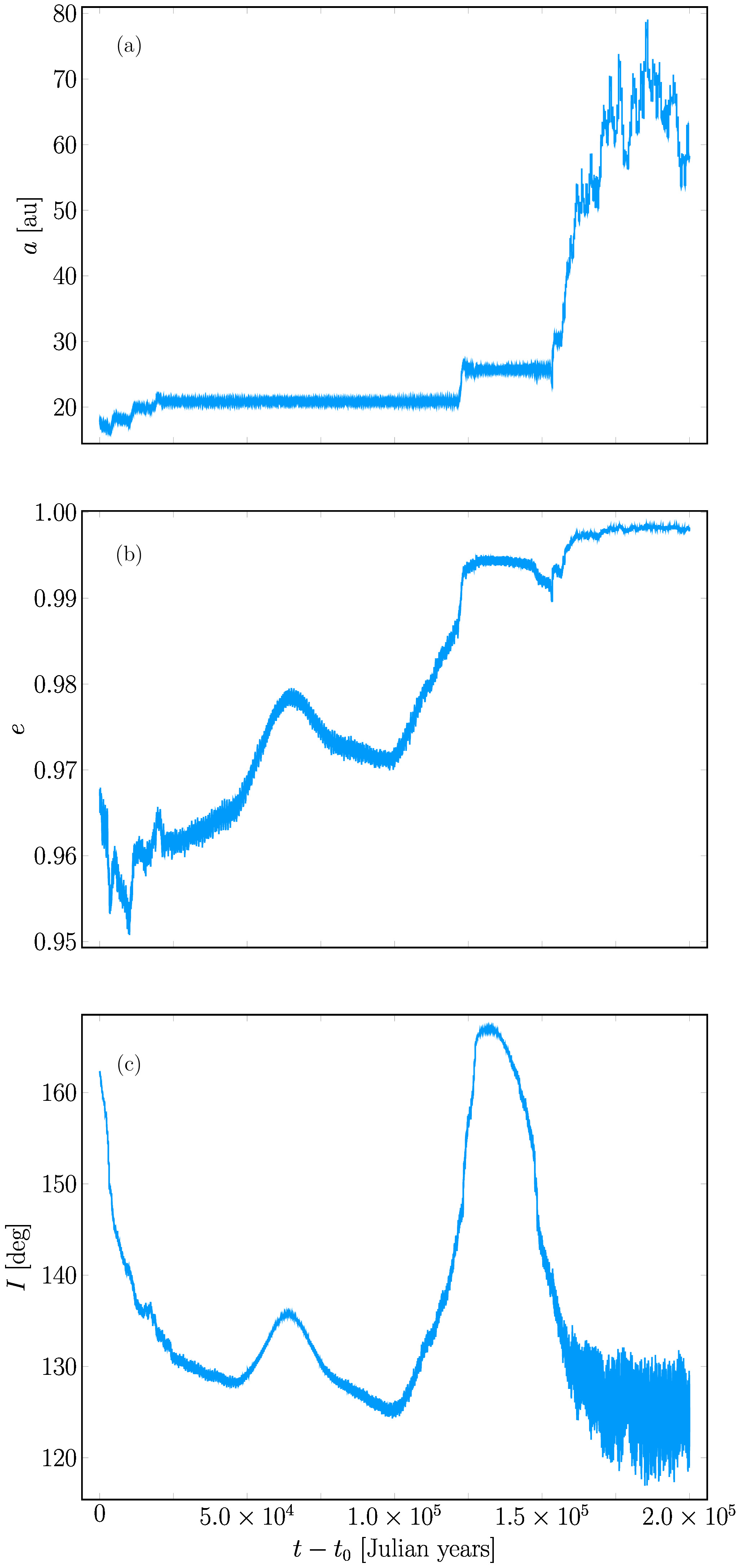
Figure 1: (a) Semi-major axis, (b) eccentricity and (c) inclination of Halley’s comet orbit as a function of time, obtained using the nominal initial conditions defined at $t_{0}=2449400.5$ JD (February 17, 1994).

Within the first few thousand years, Figs. 1 display some sudden changes in the semi-major axis, eccentricity and inclination of Halley’s orbit. These events display the accumulation effects of close approaches with Jupiter; in particular, an important one occurs at $t-t_{0}\simeq 2925$ yr, in which Halley’s comet enters the Hill radius of Jupiter reaching a minimum distance of $\sim 0.445$ $\rho_{\textrm{J}}$, where $\rho_{\textrm{J}}\approx 0.355$ au is Jupiter’s Hill radius. This event was already pointed out by Muñoz-Gutiérrez et al. (2015). Boekholt et al. (2016) noticed an important role played by Venus during the first $\sim 3\times 10^{3}$ yr; we confirm the occurrence of some approaches to Venus during that time, the closest one occurring around $t-t_{0}\simeq 732$ yr, with the comet being within a distance $\sim 8.08\rho_{\textrm{V}}$ from the planet, where $\rho_{\textrm{V}}\approx 6.76\times 10^{-3}$ au is Venus’ Hill radius. Those close approaches lead to sudden increments of the semi-major axis, which display oscillations of $\sim 1$ au. Eventually, Halley’s comet semi-major axis oscillates in a seemingly steady form around $a\approx 21$ au for a long time ($\sim 10^{5}$ yr), avoiding close encounters with Jupiter. During that time, the eccentricity and inclination still display changes, in particular a marked bump reaching $e\sim 0.98$ and $I\sim 135^{\circ}$, which we interpret as the effect of the accumulation of secular instabilities. This bump is followed by an abrupt increase in the eccentricity and inclination, this time due to a close approach with the Sun. Beyond $t-t_{0}\gtrsim 1.1\times 10^{5}$ yr, these instabilities allow new close encounters with Jupiter and the Sun which make the eccentricity attain rather large values, $e\sim 0.998$, induce a clear increment of the semi-major axis, and a drastic reduction of the inclination, which also displays larger fluctuations. The large values of the eccentricity attained suggest the possibility of an eventual ejection of Halley’s comet from the Solar System; we shall return later to this observation.

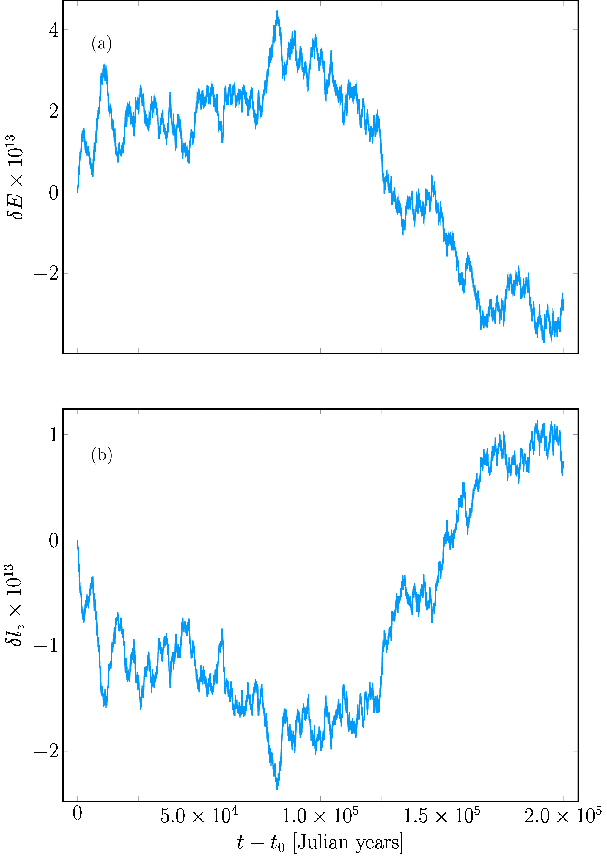
Figure 2: (a) Relative variation of the total energy and (b) $z$-component of the total angular momentum of the Solar System (Sun and planets) as a function of time.

Regarding the quality of our integration, in Figs. 2 we display the relative change of the total energy of the Solar System with respect to its initial value, $\delta E$, and the corresponding relative change of the $z$-component of the angular momentum of the Solar System, $\delta l_{z}$, as functions of time. As illustrated, we obtain $|\delta E|\leq 3\times 10^{-13}$ and $|\delta l_{z}|\leq 1.1\times 10^{-13}$. The overall behavior of these relative changes resembles a random walk; this is a consequence of the error per time step of our integrations being essentially the machine round-off error. These figures show that accumulation of those errors over the integration time are small and close to the initial energy and angular momentum values, which are the dynamical constraints imposed by the integrals of motion. While these results are independent of the presence of Halley’s comet, which is treated as a massless particle, they do influence the motion of the comet through their presence in Eq. 6; small errors in the preservation of the integrals of motion in the $N$-body problem are considered more trustworthy numerical results (Zwart & Boekholt, 2014).

4.2 Fourier analysis: Power spectrum

In order to further understand Halley’s dynamics in more detail, we have computed the discrete Fourier Transform associated to the time series defined by the Halley’s osculating orbital elements displayed in Figs. 1, from which we obtain the associated power spectra. We denote by $S_{a}(f)$, $S_{e}(f)$ and $S_{I}(f)$ the power spectra associated to Halley’s semi-major axis, eccentricity and inclination, respectively. In Figs. 3 we present the results as a function of the frequency, in log-log scale. In these figures, the vertical dashed lines correspond to the current planetary orbital frequencies, including also $2f_{\mathrm{Ju}}$; table 1 includes the values of the planetary orbital periods and the corresponding orbital frequencies. In these figures we have additionally indicated the $1/f^{2}$ decay, which serves to distinguish any important feature from the bulk. The figures clearly show a broadband component which are a clear manifestation of the chaotic dynamics (Sussman & Wisdom, 1988) of comet Halley.

Figure 3(a) shows an important accumulation of peaks located around Jupiter’s orbital frequency $f_{\mathrm{Ju}}$, which clearly form a bump. There is also a much smaller bump around Mars frequency $f_{\mathrm{Ma}}$, and a small peak coinciding with the present orbital frequency of Venus, $f_{\mathrm{Ve}}$. These features reflect the increment of the semi-major axis displayed by Halley’s orbit, illustrated in Fig. 1(a), due to different close approaches.

Likewise, in Figs. 3(b) and 3(c), $S_{e}(f)$ and $S_{I}(f)$ display some peaks that match the planetary orbital frequencies of all planets, except for Uranus and Neptune in the case of $S_{e}(f)$. The strongest peaks with respect to the background (the $1/f^{2}$ line) correspond to the frequencies clustered around Jupiter’s current frequency, though the frequencies of Saturn ($f_{\mathrm{Sa}}$), Venus ($f_{\mathrm{Ve}}$) and the Earth ($f_{\mathrm{Ea}}$) seem also to play a significant role. We also note the approximate $1:6$ commensurability among the frequencies of Jupiter and Halley’s comet, i.e., $f_{\mathrm{Ju}}\approx 6f_{\mathrm{Ha}}$ (Sekhar & Asher, 2014). The appearance of some peaks between the frequencies of Mars and Jupiter is associated to harmonics of this approximate resonance; notice in particular that $S_{I}(f)$ displays contributions of the $2:12$ and $3:18$ harmonics. Using the relative height of the resonance peaks with respect to the local power spectrum signal, Jupiter, Saturn, Venus and the Earth seem to be the main perturbers of Halley’s eccentricity and inclination.

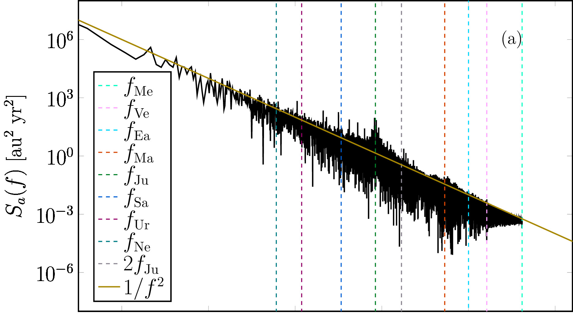
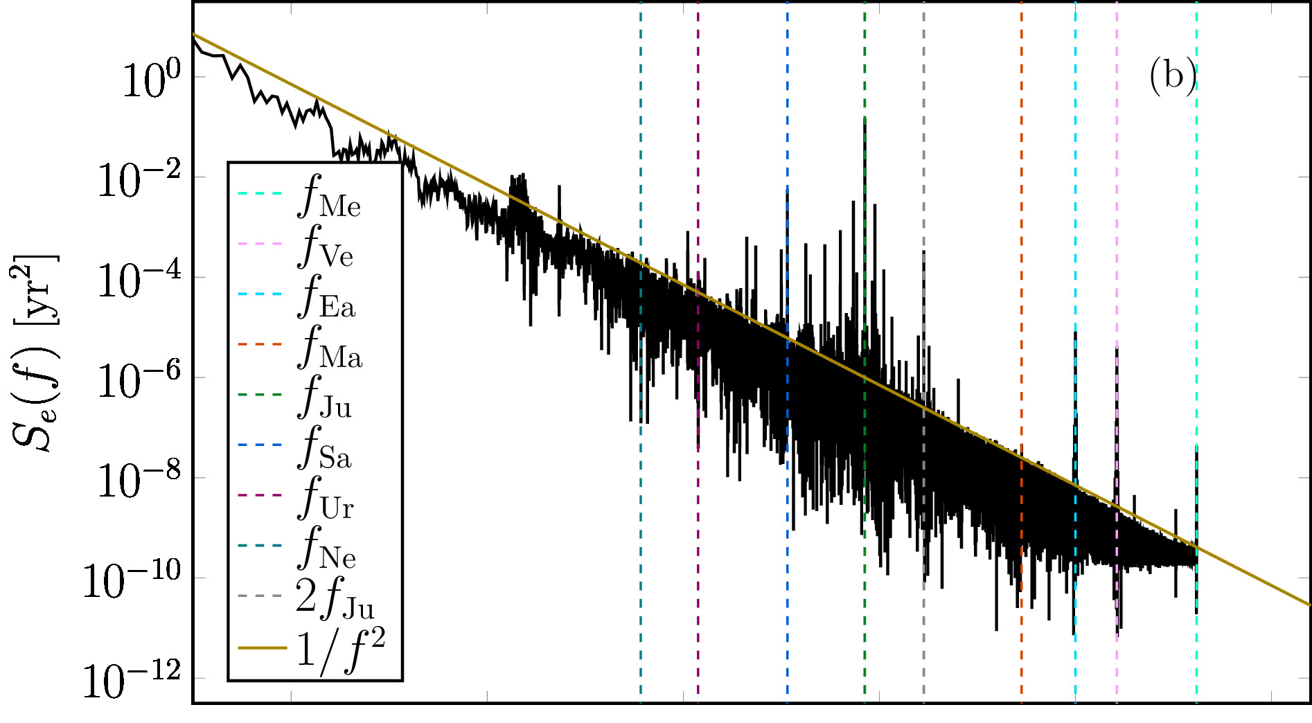
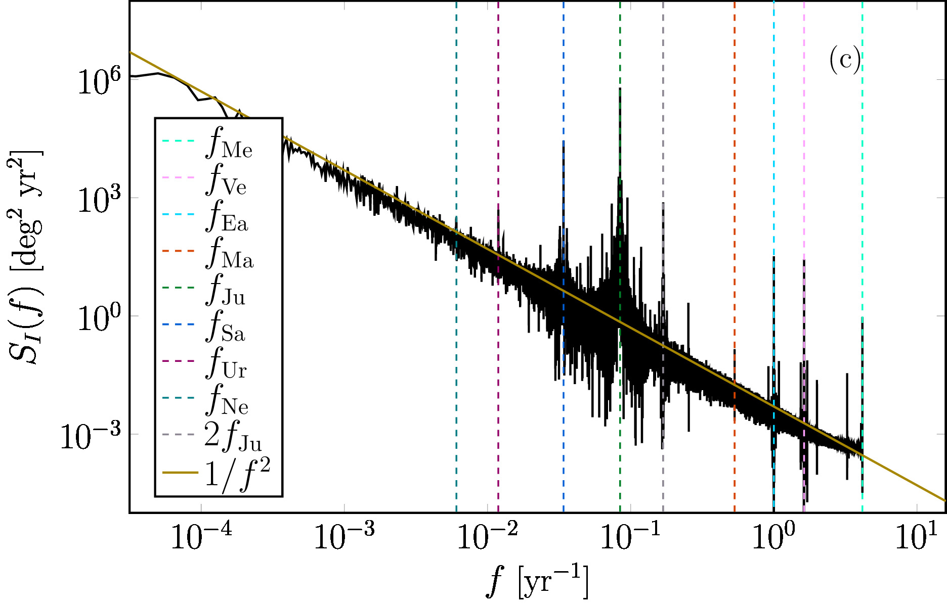
Figure 3: Power spectrum (a) $S_{a}(f)$, (b) $S_{e}(f)$ and (c) $S_{I}(f)$ (black) associated to Halley’s osculating semi-major axis, eccentricity and inclination, computed over $2\times 10^{5}$ yr. Vertical dashed lines correspond to current planetary orbital frequencies as indicated in the legend. The figures include the $1/f^{2}$ decay to separate any interesting feature from the bulk.

4.3 Lyapunov spectrum

We consider now the Lyapunov spectrum of Halley’s orbit. In Fig. 4(a) we present the time dependence of each of the six Lyapunov exponents of Halley’s orbit using a linear scale; Fig. 4(b) displays in a log-log scale the absolute value of the Lyapunov exponents, excluding the maximum one, $\lambda_{1}$, and the minimum one, $\lambda_{6}$. Clearly, only $\lambda_{1}$ and its time-reversal partner $\lambda_{6}$ seem to attain asymptotically non-zero values. The upper bound of the absolute value of the remaining exponents tends to zero as a power law in time, seemingly as $t^{-1/2}$, though important fluctuations are observed. That is, along the orbit of the comet there is one (time-dependent) direction in phase space where the instabilities and thus chaos are particularly strong, another one corresponding to its time-reversal (stable) counterpart, and the remaining independent directions behave asymptotically as neutral directions with respect to long-term stability. Therefore, small deviations in the initial conditions which are not perfectly perpendicular to the single unstable direction will display sensitivity to the initial conditions.

We address now the validity of the calculations of the Lyapunov exponents presented. In Fig. 5 we display the time dependence of the sum of the Lyapunov exponents. As noted above, Eq. (12) permits to check how the symplectic structure of the equations of motion for Halley’s comet is preserved by the integration. Figure 5 illustrates that the variations of $\sum_{i}\lambda_{i}$ remain very close to zero for all times, and are essentially due to the accumulation of round off errors in each time-step of the integration. We emphasize that Taylor’s method is not symplectic; yet, by using polynomials of high-enough order and a small enough tolerance $\varepsilon$, the method preserves numerically the symplectic structure.

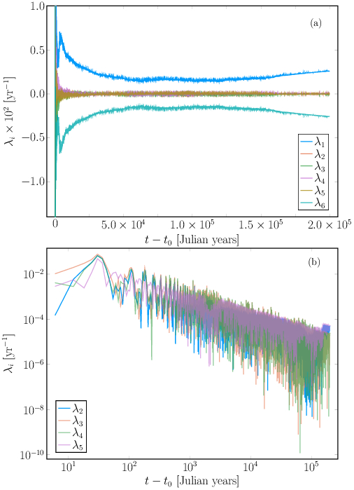
Figure 4: Time dependence of the Lyapunov spectrum: (a) All exponents are displayed in linear scale; (b) absolute value of all exponents except for the maximum Lyapunov exponent $\lambda_{1}$, and its time-reversal partner, $\lambda_{6}$, in log-log scale. We notice that the exponents included in (b) display a convergence to zero in time, seemingly as $t^{-1/2}$.

Figure 4(a) shows that, despite of the fact that the maximal Lyapunov exponent $\lambda_{1}$ is non-zero, it has not yet attained convergence during the integration time considered. This is apparent by the increasing tendency displayed during the last $4\times 10^{4}$ yr of our integration. In order to have an estimate of the Lyapunov time, we consider the average value of the maximum Lyapunov exponent for times $t-t_{0}\geq 5\times 10^{4}$ yr. This criterion is chosen because the changes of $\lambda_{1}$ seem to remain relatively constant during this time interval, except for the last $4\times 10^{4}$ yr of the orbit. We obtain $\overline{\lambda_{1}}=1.777\times 10^{-3}$ yr^-1, with the minimum and maximum values corresponding to $1.424\times 10^{-3}$ yr^-1 and $2.597\times 10^{-3}$ yr^-1. From the average value, our estimate of the Lyapunov time for Halley’s comet is $\tau_{L}=1/\overline{\lambda_{1}}\simeq 562$ yr. This result is larger than the values reported by Muñoz-Gutiérrez et al. (2015), $\tau_{L}\sim 70$ yr, and Boekholt et al. (2016), $\tau_{L}\sim 300$ yr.

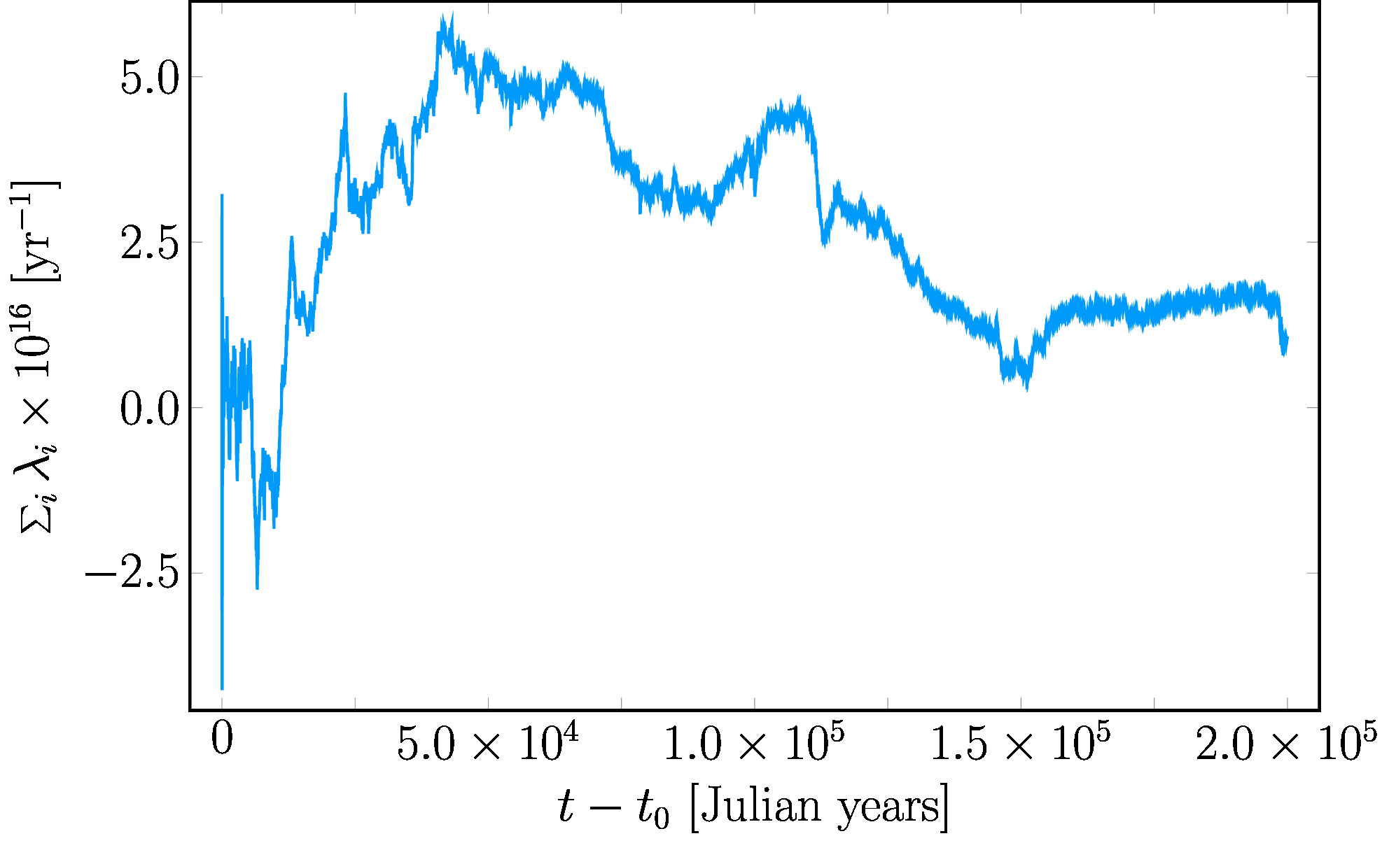
Figure 5: Time dependence of the sum of the Lyapunov exponents, as a test of the preservation of the symplectic structure of the equations of motion by our integration method.

5 Discussion

In view of the different results obtained for $\lambda_{1}$, it is worth describing the differences of all models that are under comparison. First, the initial conditions used are all different as well as the numerical methods employed. These are important due to the underlying chaotic dynamics of comet Halley. The Solar System models used are also different, though all include only Newtonian gravitational interactions: Muñoz-Gutiérrez et al. (2015) include all planets except for Mercury, whose mass is added to the Sun, five dwarf planets and five minor bodies. In turn, Boekholt et al. (2016) use all planets as we do, except for the inclusion of the Moon. The time scales spanned by the calculations are also different, ours being the longest. Finally, the actual methods used to compute the maximal Lyapunov exponents are different. As noted by Boekholt et al. (2016), Muñoz-Gutiérrez et al. (2015) use the iterative scheme proposed by Benettin et al. (1976), while they measure directly the rate of exponential growth from the separation of the two orbits. We note that both groups use fiducial orbits in their calculations. Our method is based on the numerical integration of the first variational equations (Benettin et al., 1980b) which avoids the use of any fiducial orbit and thus is not subject to artificial overestimations (Tancredi et al., 2001), though this method is computationally more demanding.

The lack of convergence of $\lambda_{1}$ (and $\lambda_{6}$), manifested in the last $4\times 10^{4}$ yr of our integration, seems reminiscent of early findings for the maximum Lyapunov exponent of the Jupiter family comets (Tancredi, 1995). There, it was observed that some Lyapunov exponents seemed to converge up to a certain time, followed by a sudden change associated to the orbit crossing a partial dynamical barrier (cantorus) in phase space, which increased the value of the calculated Lyapunov exponent. This behavior was attributed to (recurrent) close encounters of the comets with Jupiter (Tancredi, 1995) which allowed the comets to escape from a phase-space region with reduced diffusion (sticky region) to one with enhanced diffusion (Contopoulos & Barbanis, 1989). We do observe the impulsive close approaches with different bodies in our simulations, but still with no convergence of the Lyapunov exponent.

Convergence in the limit of infinite time is expected by Osedelet’s theorem (Oseledet, 1968). Disregarding the lack of its applicability —since there are clear indications of irregular motion—, the lack of convergence of the Lyapunov exponents could be attributed to the finite, and perhaps short, integration time considered. While this is certainly a limitation, the Lyapunov time obtained is much shorter than the total time-scale of our integration, from which convergence could be expected. Another alternative to understand the lack of convergence is that comet Halley will eventually escape. This is possible through the accumulation of close encounters which cause sudden changes in the osculating orbital elements and in the value of the Lyapunov exponents, as shown in Figs. 1 and 4. Noticing that towards the end of our integration the computed orbit displays values for the eccentricity that are very close to 1, close approaches with the Sun are expected essentially once per orbital period. These encounters are an efficient mechanism for ejection, which leads us to conclude that comet Halley will eventually escape from the Solar System. From our integration, the closest approach of comet Halley to the Sun occurs at $t-t_{0}\approx 1.776\times 10^{5}$ yr, at a distance $\sim 0.134$ au, that is, about $1/3$ the current semi-major axis of Mercury, i.e. $\sim 30~{}R{}_{\odot}$.

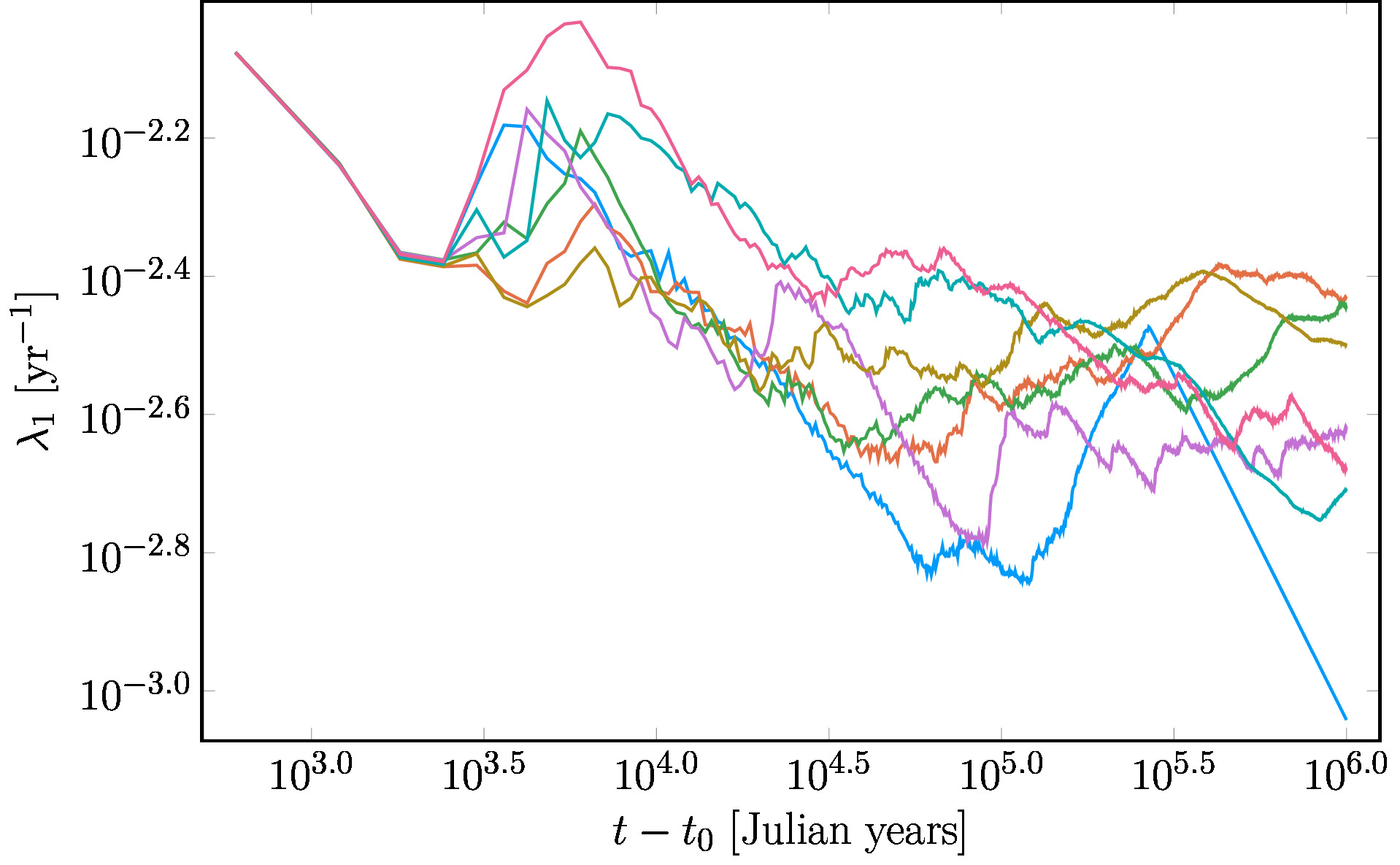
Figure 6: Time dependence of maximum Lyapunov exponent $\lambda_{1}$, during $1\times 10^{6}$ yr, of the nominal Halley orbit (blue line), and 6 nearby initial conditions.

If the comet escapes, the dynamics become integrable in the asymptotic region, as the comet will only feel the interaction with the Sun, with a mass corrected to include the other Solar System bodies, i.e., after escape the dynamics corresponds essentially to the two-body problem. In this case, the complex dynamics displayed by Halley’s comet are only temporary, limited in time, and in that sense a manifestation of chaotic scattering or transient chaos (Ott & Tél, 1993; Lai & Tél, 2011). Then, all Lyapunov exponents converge to zero due to integrability of the asymptotic dynamics, where the particle escapes as $t^{2/3}$. We note that this is in agreement with Osedelet’s theorem. Accordingly, finite-time estimations of the Lyapunov time $\tau_{L}$ in the vicinity of comet Halley’s nominal orbit display a lack of convergence, different time dependence and values, being highly dependent on the initial conditions as well as the propagation of numerical errors. Since convergence is not reached, the computed values of $\tau_{L}$ are transient and hard to interpret, and it is not clear to us if they entail any significance.

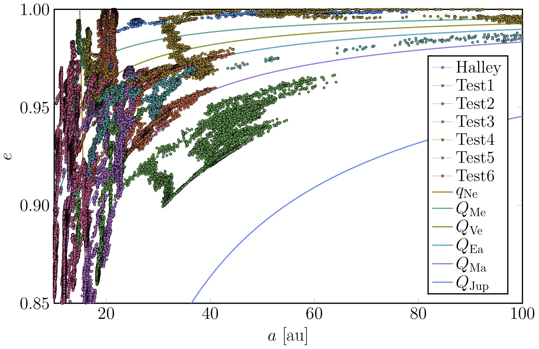
Figure 7: Evolution of Halley’s comet semimajor axis and eccentricity $(a,e)$ at each perihelion passage, computed over $1\times 10^{6}$ yr, for each of the orbits in Fig. 6. Solid curves show the values of the pair $(a,e)$ corresponding, respectively, to the perihelia ($Q$) and aphelia ($q$) of Mercury, Venus, Earth, Mars, Jupiter and Neptune.

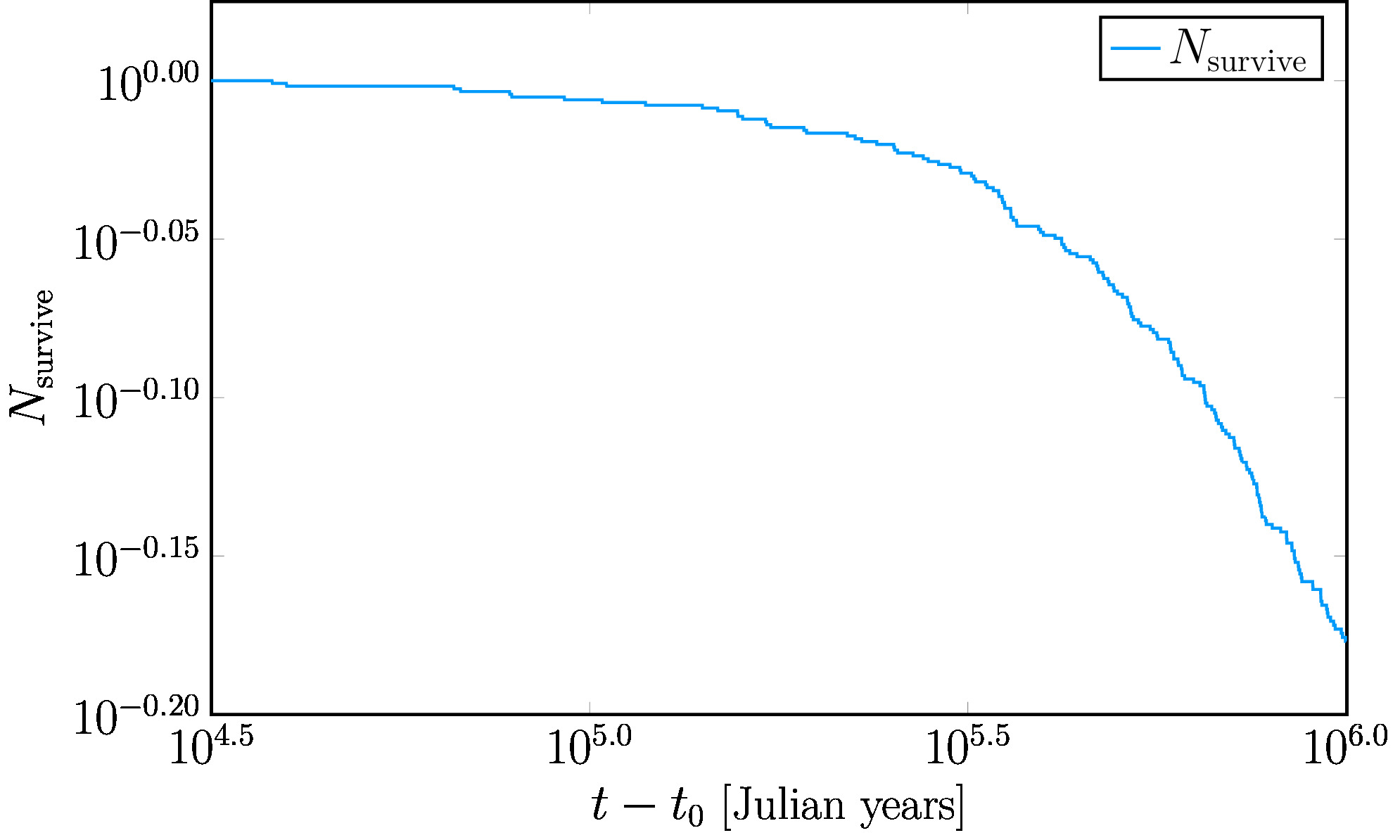
Figure 8: Decay of the survival probability of 508 initial conditions considered at random, within a sphere of $150$ km centered at the nominal position of Halley’s comet.

To illustrate this conclusion, we integrate comet Halley’s nominal orbit, as well as 6 nearby initial conditions, during $1\times 10^{6}$ yr. Figure 6 shows the maximum Lyapunov exponent $\lambda_{1}$ associated to each of those initial conditions. The perturbed initial conditions differ by $150$ km in the initial position with respect to the nominal orbit. We observe that the nominal orbit (light blue) does indeed escape after $\sim 2\times 10^{5}$ yr, when the comet’s orbit becomes hyperbolic. This is manifested in Fig. 6 as $\lambda_{1}$ converging to zero, seemingly as $t^{-1}$. From our results, the escaping time for the nominal initial conditions is about $2.7\times 10^{5}$ yr. Furthermore, we note that while the rest of the integrated orbits shown in Fig. 6 do not escape the Solar System within $1$ Myr, their maximum Lyapunov exponents do not display convergence either. We also notice in Fig. 6 that the maximum Lyapunov exponent of the computed trajectories have the same value up to $\sim 2.72\times 10^{3}$ yr, and afterwards they evolve independently. This is related to a close approach to Jupiter, in which the comet almost enters the Hill sphere of the planet. In Fig. 7 we plot, in the $a$–$e$ plane, the evolution of the osculating elements at perihelion passage for each of the orbits shown in Fig. 6. Clearly, there is a long-term sensitivity of the osculating elements to perturbations of the initial condition, as evidenced by the different regions visited, where we observe that three of the computed trajectories reach $100$ au for the semi-major axis with quite high eccentricity.

In order to characterize the rate of escape of the vicinity of comet Halley’s orbit, we consider 508 initial conditions close to the nominal orbit, and integrate them up to $1\times 10^{6}$ yr. Figure 8 shows the fraction of initial conditions $N_{\mathrm{survive}}$ which have not escaped at time $t$. The sampled initial conditions are obtained by varying the initial position of the test particle within a radius of $150$ km, which is essentially the uncertainty of comet Halley’s semimajor axis (Landgraf, 1986). The escape condition requires that the comet’s orbit is hyperbolic in a Keplerian sense, that is, that $e>1$ and its Keplerian energy is positive. We notice that these results are consistent with the structure of the survival maps of Halley’s comet (Muñoz-Gutiérrez et al., 2015), and manifest that the escape time is highly sensitive to the initial conditions and the propagation of numerical errors (Benet et al., 1998, 2005). We thus conclude that comet Halley will likely escape from the Solar System, and $\lambda_{1}$ will display non-converging transient behavior until the comet escapes, after which $\lambda_{1}\to 0$.

6 Conclusions

In this paper, using a purely Newtonian model for the Solar System, we have computed numerically the orbit of comet 1P/Halley for $2\times 10^{5}$ yr, using for the initial conditions those provided by JPL’s Horizons system, corresponding to February 17th, 1994, 00:00:00.0 (TDB). The orbit computed displays important abrupt changes due mainly to close approaches with Jupiter, though other planets influence importantly the comet’s trajectory. Secular resonances and close approaches with the Sun are also manifested.

We have studied the power spectra associated to Halley’s semi-major axis $S_{a}(f)$, eccentricity $S_{e}(f)$ and inclination $S_{I}(f)$. The power spectra display a broadband component, which is consistent with the chaotic dynamics (Sussman & Wisdom, 1988) of Halley’s orbit. The results for $S_{e}(f)$ and $S_{I}(f)$ manifest peaks associated to the current planetary frequencies, which are dominated in particular by Jupiter, Venus, Saturn and the Earth, according to the relative strength of the associated peaks with respect to the $1/f^{2}$ decay of the bulk. In addition, the $1:6$ resonance with Jupiter seems to be relevant (Sekhar & Asher, 2014) as well as some of its harmonics. Therefore, these results support that close approaches with Jupiter influence importantly Halley’s orbital elements, but also resonant interactions with other planets, including Venus, as it has been recently suggested (Boekholt et al., 2016).

We have also presented results on the Lyapunov spectrum of the comet, which has been computed integrating the variational equations. For the nominal orbit of comet Halley, we obtained for the average maximum Lyapunov exponent $\overline{\lambda_{1}}\approx 1.777\times 10^{-3}$ yr^-1, from which we estimate the Lyapunov time $\tau_{L}=1/\overline{\lambda_{1}}=562$ yr. Notice that for this value of $\tau_{L}$, an initial deviation $\delta_{0}=150$ km requires $\sim 2100$ yr to grow to the radius of the Earth. This value is larger than the previously reported (Muñoz-Gutiérrez et al., 2015; Boekholt et al., 2016), and it roughly agrees with the interval of confirmed observations of the comet. Yet, we point out that our results, up to $2\times 10^{5}$ yr, do not display convergence for $\lambda_{1}$, which is also manifested in integrations of initial conditions close to the nominal orbit of the comet. We interpret the lack of convergence of the maximum Lyapunov exponent as a signature of transient chaos, which will lead to an eventual ejection of the comet from the Solar System. Numerical computations spanning $1$ Myr confirm the escape of the nominal orbit comet as well as other neighboring trajectories.

Aside from the non-zero values of $\lambda_{1}$ and $\lambda_{6}$, the latter being the time-reversal associate of $\lambda_{1}$, and the fact that these exponents have not converged by the end of our simulations, the rest of the Lyapunov exponents seem to converge to zero asymptotically as $t^{-1/2}$. We have presented results on the total energy of the Solar System, the $z$-component of its total angular momentum, and the sum of all Lyapunov exponents, which provide good confidence checks on the numerical results obtained.

In our work, as well as in previous works (Muñoz-Gutiérrez et al., 2015; Boekholt et al., 2016) no relativistic corrections in Mercury’s orbit have been taken into account, nor during Halley’s passages through perihelia. Similarly, the non-gravitational cometary accelerations (Marsden et al., 1973) have been disregarded. It is clear that those contributions may influence the possible ejection of Halley’s comet from the Solar System; these questions remain open.

References

- Benet et al. (1998) Benet L., Seligman T., Trautmann D., 1998, Celest Mech Dyn Astr, 71, 167
- Benet et al. (2005) Benet L., Broch J., Merlo O., Seligman T. H., 2005, Phys. Rev. E, 71, 036225
- Benettin et al. (1976) Benettin G., Galgani L., Strelcyn J.-M., 1976, Phys. Rev. A, 14, 2338
- Benettin et al. (1980a) Benettin G., Galgani L., Giorgilli A., Strelcyn J.-M., 1980a, Meccanica, 15, 9
- Benettin et al. (1980b) Benettin G., Galgani L., Giorgilli A., Strelcyn J.-M., 1980b, Meccanica, 15, 21
- Boekholt et al. (2016) Boekholt T. C., Pelupessy F., Heggie D. C., Portegies Zwart S., 2016, MNRAS, 461, 3576
- Chirikov & Vecheslavov (1989) Chirikov R., Vecheslavov V., 1989, Astron. Astrophys., 221, 146
- Contopoulos & Barbanis (1989) Contopoulos G., Barbanis B., 1989, Astronomy and Astrophysics, 222, 329
- Folkner et al. (2014) Folkner W. M., Williams J. G., Boggs D. H., Park R. S., Kuchynka P., 2014, Interplanet. Netw. Prog. Rep., 196, 1
- Giorgini et al. (1996) Giorgini J. D., et al., 1996, in AAS/Division for Planetary Sciences Meeting Abstracts #28. p. 1158
- Jorba & Zou (2005) Jorba À., Zou M., 2005, Exp. Math., 14, 99
- Lai & Tél (2011) Lai Y., Tél T., 2011, Transient Chaos: Complex Dynamics on Finite Time Scales. Applied Mathematical Sciences, Springer New York
- Landgraf (1986) Landgraf W., 1986, A&A, 163, 246
- Marsden et al. (1973) Marsden B. G., Sekanina Z., Yeomans D. K., 1973, ApJ, 78, 211
- Muñoz-Gutiérrez et al. (2015) Muñoz-Gutiérrez M., Reyes-Ruiz M., Pichardo B., 2015, MNRAS, 447, 3775
- Oseledet (1968) Oseledet V. I., 1968, Trudy Moskovskogo Matematicheskogo Obshchestva, 19, 179
- Ott & Tél (1993) Ott E., Tél T., 1993, Chaos, 3, 417
- Pérez-Hernández & Benet (2018) Pérez-Hernández J. A., Benet L., 2018, TaylorIntegration.jl: ODE integration using Taylor’s method in Julia, https://github.com/PerezHz/TaylorIntegration.jl, doi:10.5281/zenodo.2562364
- Pikovsky & Politi (2016) Pikovsky A., Politi A., 2016, Lyapunov exponents: a tool to explore complex dynamics. Cambridge University Press
- Sekhar & Asher (2014) Sekhar A., Asher D. J., 2014, Meteoritics & Planetary Science, 49, 52
- Shevchenko (2007) Shevchenko I. I., 2007, in Valsecchi G. B., Vokrouhlický D., Milani A., eds, IAU Symposium Vol. 236, Near Earth Objects, our Celestial Neighbors: Opportunity and Risk. pp 15–30, doi:10.1017/S174392130700302X
- Skokos (2010) Skokos C., 2010, in , Dynamics of Small Solar System Bodies and Exoplanets. Springer, pp 63–135
- Sussman & Wisdom (1988) Sussman G. J., Wisdom J., 1988, Science, 241, 433
- Tancredi (1995) Tancredi G., 1995, Astronomy and Astrophysics, 299, 288
- Tancredi et al. (2001) Tancredi G., Sánchez A., Roig F., 2001, AJ, 121, 1171
- Urban & Seidelmann (2014) Urban S. E., Seidelmann P. K., eds, 2014, Explanatory Supplement to the Astronomical Almanac, 3rd Edition. University Science Books
- Yeomans & Kiang (1981) Yeomans D. K., Kiang T., 1981, Monthly Notices of the Royal Astronomical Society, 197, 633
- Yeomans et al. (1986) Yeomans D. K., Rahe J., Freitag R. S., 1986, J. R. Astron. Soc. Canada, 80, 62
- Zwart & Boekholt (2014) Zwart S. P., Boekholt T., 2014, The Astrophysical Journal Letters, 785, L3