Don’t be jelly:

Abstract

Jellyfish have been called one of the most energy-efficient animals in the world due to the ease in which they move through their fluid environment, by product of their morphological, muscular, and material properties. We investigated jellyfish locomotion by conducting in silico comparative studies and explored swimming performance across different fluid scales (e.g., Reynolds Number), bell contraction frequencies, and contraction phase kinematics for a jellyfish with a fineness ratio of 1 (ratio of bell height to bell diameter). To study these relationships, an open source implementation of the immersed boundary method was used (IB2d) to solve the fully coupled fluid-structure interaction problem of a flexible jellyfish bell in a viscous fluid. Thorough 2D parameter subspace explorations illustrated optimal parameter combinations in which give rise to enhanced swimming performance. All performance metrics indicated a higher sensitivity to bell actuation frequency than fluid scale or contraction phase kinematics, via Sobol sensitivity analysis, on a high performance parameter subspace. Moreover, Pareto-like fronts were identified in the overall performance space involving the cost of transport and forward swimming speed. Patterns emerged within these performance spaces when highlighting different parameter regions, which complemented the global sensitivity results. Lastly, an open source computational model for jellyfish locomotion is offered to the science community that can be used as a starting place for future numerical experimentation.

1 Introduction

Scientists have long tried to understand aquatic locomotion in organisms ranging in size and scale from phytoplankton to whales. Oftentimes, an organism’s size and shape dictates what type of locomotive process it uses to move around its fluid environment (e.g., small invertebrates such as ctenophores use ciliary based motion Pang:2008 , while larger organisms like fish may use fin-based propulsion Akanyeti:2017 ). One quantity that helps describe the scale of a fluid system is a dimensionless number called the Reynolds Number, $\mathrm{Re}$. The $\mathrm{Re}$ can be interpreted as the ratio of inertial to viscous forces, thus categorizing the importance of viscous effects on the behavior of the underlying fluid system. It can be mathematically represented by

$$\mathrm{Re}=\frac{\rho VL}{\mu}=\frac{\rho fL^{2}}{\mu},$$ (1)

where $\rho$ and $\mu$ are the fluid’s density and viscosity, respectively, $L$ is a characteristic length scale of the problem (e.g., such as the size of a fish fin or ctenophore’s cilia), and $V=fL$ is a characteristic velocity scale, which could be the speed of a fish fin or ctenophore’s cilia during it’s stroke cycle. Although in their natural environments a salt water fish and ctenophore are immersed within approximately the same fluid (e.g., same density and viscosity), they use considerably different modes of locomotion (mechanisms) to move through their fluid environment. There are evolutionary processes which selected and developed particular locomotive mechanisms. Many such mechanisms are largely based on the size of the organism, e.g., length scale of the problem Vogel:1996 .

Recently, scientists have been trying to understand how jellyfish, the most energy-efficient animals in the world Gemmell:2013 ; Costello:2020 , swim. Jellyfish are soft body marine organisms composed of gelatinous bell, tentacles containing nematocists for prey capture, and either 4 or 8 oral arms Hamlet:2012 ; Santhanakrishnan:2012 . Their nervous system typically consists of a distributed net of cells, which are concentrated into small structures called rhopalia Gemmell:2014 . There are between four and sixteen rhopalia around the rim of the bell, which coordinate muscular contraction to propel the jellyfish forward Satterlie:2011 . Their relatively simple morphology and nervous systems make them attractive to robotocists Joshi:2012 ; Frame:2018 ; Christianso:2019 ; Ren:2019 ; Costello:2020 . In 2020, a bio-hybrid robot was introduced that could swim up to 2.8 times faster than the natural swimming speeds of the actual jellyfish to which the microelectronics were planted. It was able to do this while requiring 10-1000 times less power per unit mass than other aquatic robots Xu:2020 .

Outside of laboratory settings, many computational scientists have developed computational fluid dynamics (CFD) models of jellyfish that produce forward propulsion Dular:2009 ; Wilson:2009 ; Sahin:2009a ; Sahin:2009b ; Lipinski:2009 ; Rudolf:2010 ; Hershlag:2011 ; Wilson:2011 ; Alben:2013 ; Gemmell:2013 ; Park:2014 ; Yuan:2014 ; Park:2015 ; Hoover:2015 ; Hoover:2017 ; Hoover:2019 ; Miles:2019b ; Pallasdies:2019 and have compared swimming performance over a large mechanospace of bell flexibility, muscular contraction strength, and contraction kinematics. Computational studies are attractive to scientists as it is easier (e.g., more cost and time efficient) to do parameter studies using computational models rather than building many robots or physical models. Some scientists have begun producing robust multi-scale models, whether in 2D or 3D, that couple the underlying electrophysiology to muscular force generation that results in propulsion forward Hoover:2017 ; Hoover:2019 ; Pallasdies:2019 . While these models incorporate a multitude of biological data, they inherently come with the expense of more modeling degrees of freedom, i.e., parameters.

On the other hand, there is still much to be learned about jet propulsion from simple 2D CFD actuator models of jellyfish. Hoover et al. 2015 Hoover:2015 demonstrated enhanced swimming performance when bells were driven at their resonant frequencies. Peng and Alben 2012 Peng:2012 and Alben et al. 2013 Alben:2013 illustrated how variations in bell contraction kinematics could result in substantially different swimming behavior. However, these studies did not investigate performance across different fluid scales ($\mathrm{Re}$) or extensively explore swimming performance across large parameter subspaces. Studying these mechanisms across different scales could provide more context into the behavior of some jellyfish, to whom exhibit a jet propulsion mode of locomotion only during development. After maturing (when their bells grow wide enough), they switch to a more efficient swimming mode - jet-paddling or rowing McHenry:2003 ; Weston:2009 ; Blough:2011 . Furthermore, 2D models of prolate jellyfish (the jellyfish who use jet propulsion) have shown both qualitative and quantitative agreement with experimental data Sahin:2009b ; Hershlag:2011 ; Alben:2013 ; Kakani:2013 , making it more feasible to perform widespread parameter studies than their 3D computational model counterparts.

In this work, we used an open-source implementation of the immersed boundary method, IB2d Battista:2015 ; BattistaIB2d:2017 ; BattistaIB2d:2018 , to model jellyfish locomotion using a fully coupled fluid-structure interaction framework in 2D. In particular, we modified the simple actuator model from Hoover et al. 2015 Hoover:2015 and performed comparative studies across different fluid scales (i.e., varying Reynolds Number, $\mathrm{Re}$), bell contraction frequencies ($f$), and contraction (and expansion) phase kinematics (quantified by a kinematic parameter, $p$). The parameter $p$ gives the fraction of the overall bell actuation cycle in which the bell was actively contracting. Thus, we varied three parameters ($\mathrm{Re},f,p$) and thoroughly (intensely) explored 2D parameter subspaces consisting of ($\mathrm{Re},f$), ($\mathrm{Re},p$), and ($f,p$). Each 2D subspace was explored three times, each corresponding to a different value of the third free parameter. Furthermore, global sensitivity analysis was performed via Sobol sensitivity analysis to isolate which parameter(s) most significantly affected jellyfish swimming performance, as first posited by Dabiri & Gharib 2003 Dabiri:2003 , but had yet to have been quantified. A model is called sensitive to an input parameter if small variations in the parameter result in great changes in the system’s output. Global sensitivity analyses attempt to quantify the impact of variations among the input parameters on the overall model output(s) in a holistic fashion Saltelli:2002 , as opposed to only local sensitivity measures Link:2018 ; Saltelli:2019 . The resulting performance data from the Sobol analysis was projected onto 2D subspaces for comparative purposes. Lastly, Pareto optimal-like fronts were identified across the performance space between cost of transport and forward swimming speed Eloy:2013 ; Verma:2017 ; Smits:2019 . These data exhibited qualitative agreement with the sensitivity results.

In addition, we offer the science community the first open-source jellyfish locomotion model in a fluid-structure interaction framework. It can be found at github.com/nickabattista/IB2d in the sub-directory:

IB2d$/$matIB2d$/$Examples$/$Examples$\_$Jellyfish$\_$Swimming$/$Hoover$\_$Jellyfish.

2 Mathematical Methods

To model a flexible jellyfish bell immersed in a viscous, incompressible fluid, we used a fluid-structure interaction (FSI) framework. In particular, we used an implementation of the immersed boundary method (IB), which was first conceived in the 1970s by Charles Peskin Peskin:1972 ; Peskin:1977 ; Peskin:2002 . The immersed boundary method has since been improved upon numerous times Fauci:1993 ; Lai:2000 ; Cortez:2000 ; Griffith:2005 ; Mittal:2005 ; Griffith:2007 ; BGriffithIBAMR ; Griffith:IBFE and is still a leading numerical framework for studying problems in FSI due to its robustness, simplicity, and flexibility in modelling complex deformable structures, like many that arise in biological contexts BattistaIB2d:2017 ; BattistaIB2d:2018 .

It has previously been applied to study problems ranging from cardiac fluid dynamics Miller:2011 ; Griffith:2012b ; Battista:2017 ; Battista:2020 to aquatic locomotion Bhalla:2013a ; Bhalla:2013b ; Hamlet:2015 to insect flight Miller:2004 ; Miller:2005 ; SJones:2015 to parachuting Kim:2006 to dating and relationships BattistaIB2d:2017 . Additional details on the IB method are provided in the Appendix A.

Below we will discuss the implementation of the jellyfish locomotion model in the open-source IB2d framework, i.e., the computational geometry, geometrical and fluid parameters, and model assumptions. Our model is based on the $2D$ jellyfish locomotion model of Hoover et al. 2015 Hoover:2015 whose model was implemented in the open-source IB software called IBAMR BGriffithIBAMR . IBAMR is parallelized IB software with adaptive mesh refinement MJBerger84 ; Roma:1999 ; Griffith:2007 .

2.1 Computational Parameters

In this study, we used the frequency-based Reynolds number, $\mathrm{Re}$, to describe the locomotive processes of a jellyfish. The characteristic length, $D_{jelly}$, is set to the bell diameter at rest and the characteristic frequency, $f_{jelly}$, is set to the actuation (stroke) frequency. Therefore our characteristic velocity scale is set to $V_{jelly}=f_{jelly}D_{jelly}$, as in Eq.(1),

$$Re=\frac{\rho f_{jelly}D_{jelly}^{2}}{\mu}.$$ (2)

Fluid parameters (density and dynamic viscosity) can be found in Table 1. Across all studies the dynamic viscosity, $\mu$, was selectively chosen to give a specific $\mathrm{Re}$ value, for a particular contraction frequency, $f$. The jellyfish bell’s diameter and height remained the same for all simulations performed and were chosen such that the jellyfish’s fineness ratio (the ratio of bell height to bell diameter) was exactly equal to $1.0$ Dabiri:2007 . This allowed us to investigate performance of the jet propulsive locomotion mode directly at the interface between oblate and prolate jellyfish, which have a fineness ratio of less than one and greater than one, respectively. Prolate jellyfish are known to use jet propulsion, while oblate use a jet-paddling propulsion mode Dabiri:2007 . One such jellyfish with a fineness ratio of $\sim 1$ is Catostylus mosaicus, the blue blubber jellyfish. However, our study did not explicitly attempt to model this jellyfish due to its complex oral morphology Neil:2018b , which accounts for a larger proportion of the jellyfish’s mass than other species Arai:1997 . Previous studies have shown that the addition of tentacles or oral arms can substantially affect swimming performance Katija:2015 ; Miles:2019b . Here we restricted our focus on the locomotion performance via jet propulsion on the bell alone.

Parameter	Variable	Units	Value
Domain Size	$[L_{x},L_{y}]$	m	$[5,12]$
Spatial Grid Size	$dx=dy$	m	$L_{x}/320=L_{y}/768$
Lagrangian Grid Size	$ds$	m	$dx/2$
Time Step Size	$dt$	s	$10^{-5}$
Total Simulation Time	$\mathscr{T}$	pulses	$8$
Fluid Density	$\rho$	$kg/m^{3}$	$1000$
Fluid Dynamic Viscosity	$\mu$	$kg/(ms)$	varied
Bell Radius	$a$	m	$0.5$
Bell Diameter	$D$ ($2a$)	m	$1.0$
Bell Height	$h$	m	$1.0$
Contraction Frequency	$f$	$1/s$	varied
Actuation Period	$T=1/f$	$s$	varied
Contraction Phase Fraction	$p$		varied
Spring Stiffness	$k_{spr}$	$kg\cdot m/s^{2}$	$1\times 10^{7}$
Beam Stiffness	$k_{beam}$	$kg\cdot m/s^{2}$	$2.5\times 10^{5}$
Muscle Spring Stiffness	$k_{muscle}$	$kg\cdot m/s^{2}$	$1\times 10^{5}$

Table 1: Numerical parameters used in the two-dimensional simulations.

For all simulations performed and analyzed, periodic boundary conditions were used on all edges of the computational domain and the computational width was kept constant with $L_{x}=5.$ Convergence studies demonstrated low relative errors in swimming speeds for domain sizes from $L_{x}\in[3,8]$ for $Re=\{37.5,75,150,300\}$, see Figure 15 in Appendix B. Amongst all cases, a similar trend was observed where narrower computational domains led to slightly decreased forward swimming speeds while qualitative differences vortex formation were minimal, see Figure 16 in the same appendix. Additional grid resolution convergence studies were performed in Battista & Mizuhara 2019 BattistaMizuhara:2019 using the same $2D$ jellyfish computational model that demonstrated appropriate convergence rates in both the Eulerian (fluid) and Lagrangian (jellyfish) data for the numerical parameters described in Table 1.

2.2 Jellyfish Computational Model

The geometry was composed of a semi-ellipse of semi-major axis, $b=0.75$, and semi-minor axis, $a=0.5$, see Figure 1. Note that the overall height of the bell was $h=1.0$, thus the bell was composed of more than only a hemi-ellipse. As shown, it was composed of discrete Lagrangian points that were equally spaced a distance $ds$ apart. We note that this Lagrangian mesh was twice as resolved as the background fluid grid, i.e., $ds=0.5dx$ Peskin:2002 . This choice was made in order to minimize interpolation errors between the fluid and jellyfish grids (see Eqs. (13)-(14) in Appendix A), which typically manifest themselves as fluid leaking through the immersed structure.

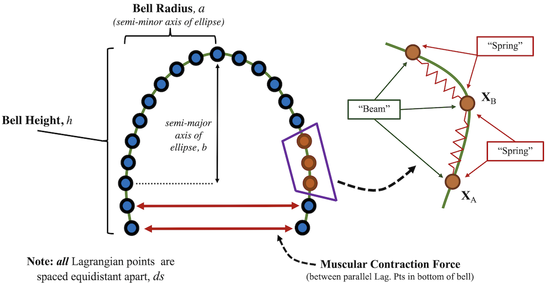
Figure 1: Jellyfish model geometry composed of discrete points is a semi-elliptical configuration. The points are connected by virtual springs and virtual beams in the IB2d.

Although one may view the jellyfish here as being immersed in the fluid, the jellyfish (Lagrangian grid) and fluid (Eulerian mesh), in an IB framework they only through integral equations with delta function kernels (see Eqs. (13)-(14) in Appendix A for more details.) In a nutshell, the Lagrangian mesh is allowed to move around and change shape. As an observer, one sees the motion of the body. On the Eulerian mesh we only measured what is happening in the fluid (velocity, pressure, external forcing) at discrete rectangular lattice points. In the latter, it is as though we had a number of measurement tools that were only checking the fluid at the precise locations where the tools were placed; we did not track individual fluid blobs. The integral equations with delta function kernels simply say that the fluid points (on the rectangular Eulerian mesh) nearest the jellyfish (on the moving Lagrangian mesh) feel the movement of the jellyfish the most (via a force), as compared to locations in the fluid grid far away (Eq. (13)). A similar analogy describes how the jellyfish feels the effect of the fluid motion by the fluid grid points nearest the jellyfish (Eq. (14)).

Successive points along the jellyfish were connected by virtual springs and virtual (non-invariant) beams in the IB2d framework, as illustrated in Figure 1. Virtual springs allowed the geometrical configuration to either stretch or compress, while virtual beams allowed bending between three successive points. When the geometry stretched, compressed, or bent there were elastic deformation forces that arose from the configuration not being in its preferred energy state, i.e., its initial bell configuration. Note that the beams were deemed non-invariant because the preferred configuration is non-invariant under rotations, so if the jellyfish had turned, the model would have undergone unrealistic motion due to these artifacts.

These deformation forces were computed as below,

$$\textbf{F}_{spr}=k_{spr}\left(1-\frac{R_{L}(t)}{||{\bf{X}}_{A}(t)-{\bf{X}}_{B}(t)||}\right)\cdot\left(\begin{array}[]{c}x_{A}(t)-x_{B}(t)\\ y_{A}(t)-y_{B}(t)\end{array}\right)$$ (5)

$$\textbf{F}_{beam}=k_{beam}\frac{\partial^{4}}{\partial s^{4}}\Big{(}\textbf{X}_{C}(t)-\textbf{X}^{con}\Big{)},$$ (6)

where $k_{spr}$ and $k_{beam}$ are the spring and beam stiffnesses, respectively, $R_{L}(t)$ are the springs resting lengths (set to $ds$, the distance between successive points), $\textbf{X}_{A}=\langle x_{A},y_{A}\rangle$ and $\textbf{X}_{B}=\langle x_{B},y_{B}\rangle$ are Lagrangian nodes tethered by a spring (see Figure 1). Note that $R_{L}(t)$ indicates that the resting lengths could be time dependent. $\textbf{X}_{C}(t)$ is a Lagrangian point on the interior of the jellyfish bell and $\textbf{X}^{con}$ is the corresponding initial (preferred) configuration of that particular Lagrangian point on the jellyfish bell. The spring stiffnesses were large to ensure minimal stretching or compression of the jellyfish bell itself. Through the beam formulation the bell was capable of bending and hence contracting for locomotive purposes. The $4^{th}$-order derivative discretization for the non-invariant beams is given in BattistaIB2d:2018 .

Lastly, to mimic the subumbrellar and coronal muscles that induce bell contractions, virtual springs were used. These springs dynamically changed their resting lengths over the course of the entire simulation to contract and expand the bell. Rather than tether neighboring points with virtual springs to model the muscles, we tethered points across the jellyfish bell, for all the Lagrangian points that were below the top hemi-ellipse. The deformation force equation does not change from Eq. (5) besides a different $k_{spr}$, which we called $k_{muscle}$, and now used time-dependent spring resting lengths, given by a preset function $R_{L}(\tilde{t})$. Each simulation defined the period of one complete bell actuation cycle, $T$, based off its specified $f$. Modular arithmetic was used in which we defined $\tilde{t}=t\mod T$, so that $0\leq\tilde{t}\leq T$. As $p$ denoted the fraction of the period that the bell was actively contracted, the overall time the bell was contracting during one cycle was $pT$. Hence the overall expansion time of a cycle was $(1-p)T$. Thus, $R_{L}(\tilde{t})$ could be mathematically represented as the following:

$$R_{L}(\tilde{t})=\left\{\begin{array}[]{cc}2a\cos\left(\frac{\pi\tilde{t}}{2pT}\right)&\ \ \tilde{t}\leq pT\\ 2a\sin\left(\frac{\pi}{2(1-p)T}\left(\tilde{t}-pT\right)\right)&\ \ pT<\tilde{t}\leq T\end{array}\right.$$ (7)

By introducing the kinematic control parameter, $p$, and defining $R_{L}(\tilde{t})$ as above, we were able to modify the kinematic actuation profile in a continuous manner. This allowed us to study variations in swimming performance under perturbations to the actuation kinematics in a concise manner. However, it is worthwhile to note that prolate jellyfish contract on much faster time scales than their expansion phase Ford:2000 ; Colin:2013 ; Kakani:2013 . Therefore lower values of $p$ more closely depicted prolate jellyfish kinematics. Note that for a simulation of specific parameters $(\mathrm{Re},f,p)$, each actuation cycle’s kinematics are identical to all others in that simulation.

Data was stored in $25$ equally spaced time points during each contraction cycle upon running all simulations. The following data was stored:

1. Position of Lagrangian Points

2. Horizontal/Vertical forces on each Lagrangian Point

3. Fluid Velocity

4. Fluid Vorticity

5. Fluid Pressure

6. Forces spread onto the Fluid (Eulerian) grid from the Jellyfish (Lagrangian) mesh

We then used the open-source software called VisIt HPV:VisIt , created and maintained by Lawrence Livermore National Laboratory for visualization as well as MATLAB MATLAB:2015a for post-processing all the simulation data. Figure 2 provides a visualization of some of the data produced of a single moment in time for simulation with bell actuation frequency of $f=0.5s^{-1}$ at a Reynolds Number of $150$ and equal contraction and expansion phase length, $p=0.5$.

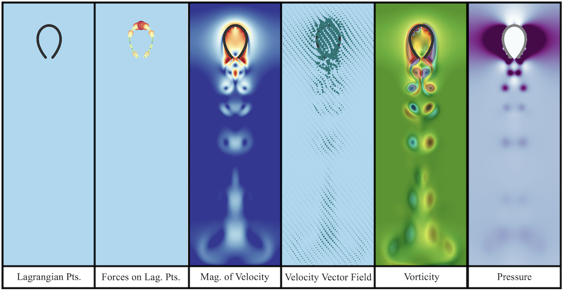
Figure 2: A snapshot of a simulation with $(\mathrm{Re},f,p)=(150,0.5,0.5)$ at the peak of contraction during its $5^{th}$ actuation cycle illustrating some of the simulation data obtained at each time-step, e.g., positions of Lagrangian points, magnitude of velocity, the velocity vector field, and vorticity. Note other data not visualized is the fluid pressure and Lagrangian forces spread from the jellyfish onto the Eulerian (fluid) grid.

We stored 25 time points per contraction cycle in each jellyfish simulation and temporally-averaged data over the 6th-8th contraction cycles to compute three swimming performance metrics - the Strouhal number ($\mathrm{St}$), a non-dimensional forward swimming speed ($1/\mathrm{St}$), and its associated cost of transport ($COT$). First, we found the average swimming speed for a particular simulation, $V_{dim}$, and used this to compute the Strouhal Number, $\mathrm{St}$,

$$\mathrm{St}=\frac{fD}{V_{dim}}$$ (8)

where $f$ is the actuation frequency and $D$ is the maximum bell diameter during an actuation cycle. The above definition of $\mathrm{St}$ used the actuation frequency rather than a vortex shedding frequency, as is commonly done in locomotion studies. Previous studies on animal locomotion have hypothesized that propulsive efficiency is high in a narrow band of $\mathrm{St}$, peaking within the interval $0.2<St<0.4$ Triantafyllou:1991 ; Taylor:2003 ; Floryan:2018 . A non-dimensional temporally-averaged forward swimming speed was then defined by taking the inverse of $\mathrm{St}$, i.e., $V=\frac{V_{dim}}{fD}=1/St$. This provided a normalized forward swimming speed based on driving frequency. We then computed the cost of transport ($COT$), which measured the energy (or power) spent per unit speed Schmidt:1972 ; Bale:2014 ; Hamlet:2015 . The dimensional COT, $COT_{dim}$ was defined as

$$COT_{dim}=\frac{1}{N}\frac{1}{V_{dim}}\displaystyle\sum_{j=1}^{N}|F_{j}||U_{j}|,$$ (9)

where $F_{j}$ was the applied contraction force at the $j^{th}$ time step by the jellyfish, $U_{r_{j}}$ was the bell contraction velocity at the $j^{th}$ time step, $N$ was the total number of time steps considered, and $V_{dim}$ was dimensional forward swimming speed during this period of time across all time steps considered. We then non-dimensionalized the cost of transport in the following manner

$$COT=\frac{COT_{Dim}}{\rho f^{2}D^{3}}.$$ (10)

The non-dimensional $COT$ calculated here was similar to the energy-consumption coefficient of Bale:2014 ; however, since $D=2a$ and $h$ are conserved across all simulations performed, only one length-scale, $D$, was used in the non-dimensionalization process.

For each simulation performed, the Strouhal number ($\mathrm{St}$), as well as a time-averaged non-dimensional forward swimming speed ($1/\mathrm{St}$) and cost of transport ($COT$) were computed. By performing simulations across highly resolved 2D subspaces of parameters, i.e., ($Re,f$), $(\mathrm{Re},p)$, and $(f,p)$, performance landscapes could effectively be mapped out. Colormap visualizations also offered the ability to qualitatively identify robust parameter subspaces that led to greater swimming performance across each subspace. Once having identified these higher performing subspaces, we sought out to perform global sensitivity analysis in order to find which parameter(s) most significantly affect the swimming performance of prolate jellyfish.

To assess this jellyfish model’s overall global sensitivity to its parameters, we used Saltelli’s extension of the Sobol sequence Saltelli:2002 ; Saltelli:2010 to form a discrete subset of parameter values of the overall parameter space in which to simulate the jellyfish. A total of M parameter combinations were selected by this process, $\{(Re,f,p)_{j}\}_{j=1}^{M}$, in which to test the model. The same swimming performance metrics ($\mathrm{St}$, $1/\mathrm{St}$, and $COT)$ were computed for each simulation upon finishing, as well as their dimensional analogs, $V_{dim}$ and $COT_{dim}$. Sobol sensitivity analysis was then performed across each performance metric. Although we mostly focused on non-dimensional performance metrics, we computed sensitivities for dimensional quantities, as well. This effort was to determine whether global parameter sensitivities for performance were substantially different across both data presentations, as global sensitivity analysis had not been previously done for jellyfish locomotion models.

Sobol sensitivity analysis is a variance-based sensitivity analysis, which provides the model’s overall global sensitivity to parameters, rather than only local sensitivity Link:2018 ; Saltelli:2019 . Global sensitivity analysis allowed us to determine which model parameter(s) most significantly caused variations in the model’s output across a specified input parameter space. It takes into account the effect of other parameters being varied in conjunction with the one of interest, thus not requiring only one parameter be varied at a time for comparative purposes. On that note, the Sobol sensitivity analysis was able to calculate both first-order parameter sensitivity indices, i.e., perturbations of one parameter at a time, higher-order indices, i.e., those corresponding to perturbations of two or more parameters at a time, and total-order indices, i.e., all combinations of other parameters Saltelli:2010 . Lastly, the importance of higher-order interactions could be determined by comparing first-order and total-order sensitivity indices. If there are significant differences between these indices, higher-order interactions are present.

Therefore the workflow of the entire Sobol sensitivity analysis process can be summarized as Figure 3 shows.

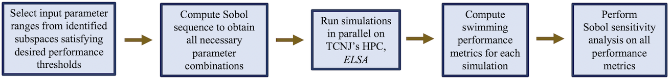
Figure 3: Workflow of the Sobol sensitivity analysis

3 Results

Different modes of locomotion are known to be more effective at certain fluid scales than others Vogel:1996 . In this work we studied the performance of the jet propulsive technique of a jellyfish with fineness ratio of $1$ across almost four orders of magnitude in $\mathrm{Re}$, within the intermediate Reynolds number regime. This is a particularly interesting (and difficult) regime to study due to the competition and balance of inertial and viscous forces Klotsa:2019 . As alluded to in past literature, swimming speed is known to be dependent on stroke (in this case, actuation) frequency Bainbridge:1958 ; Gray:1968 ; Steinhausen:2005 ; Battista:ICB2020 . Moreover, varying the contraction kinematics of prolate jellyfish have shown considerable differences in performance as well Peng:2012 ; Alben:2013 . Thus the entire 3D parameter space studied here was $\mathrm{Re}\times f\times p=[0.1,500]\times[0.25,1.25]\times[0.05,0.95].$

First, we investigated swimming performance across highly resolved 2D parameter subspaces, corresponding to the following cases:

• The ($\mathrm{Re},f$)-subspace for $3$ specific values of the kinematic parameter, $p$

• The ($\mathrm{Re},p$)-subspace for $3$ specific frequencies, $f$

• The ($f,p$)-subspace for $3$ specific Reynolds numbers, $\mathrm{Re}$.

By resolving performance across the above 2D subspaces, any nonlinear effects in performance could be parsed out of the data. Moreover, we were able to identify find robust subspaces in the parameter space which offered greater swimming performance. For this aspect of the study a total of 9,357 fully coupled 2D FSI simulations were performed.

Second, once a subspace of higher performance was identified from the above subspace explorations, we used it to initialize our parameter subspace in order to perform a formal quantitative global sensitivity analysis using Sobol sensitivity analysis. A Sobol sequence was generated using $M=1000$ and $d=3$ (the dimension of the parameter space) using Saltelli’s extension of the Sobol sequence Saltelli:2002 ; Saltelli:2010 . This gave rise to a total of $M(d+2)=5000$ different parameter combinations that would each need to be simulated in order to find the Sobol sensitivity indices of each performance metric. As global sensitivity analysis had not been previously done on jellyfish locomotion models, we applied it to both non-dimensional and dimensional performance metrics to observe whether there were any discrepancies between the two data forms.

Hence a grand total of 14,357 fully coupled 2D FSI simulations were performed using The College of New Jersey’s high performance computing cluster TCNJ:ELSA , requiring just over 1.04 million computational hours. In each simulation as the jellyfish contracts its bell, it expels a vortex ring downward, which by conservation of momentum then propels the jellyfish forward (upwards) McHenry:2007 . As the bell expands, it draws surrounding fluid up into it. Varying the three parameters of interest $(\mathrm{Re},f,p)$ can lead to substantially different swimming behavior, both in terms of kinematics as well as dynamical performance. Figure 4 shows this through snapshots corresponding to different ($\mathrm{Re},f,p$) cases by giving that case’s jellyfish position and fluid vorticity after the $5^{th}$ actuation cycle. These cases were selected as they all gave rise to pronounced forward swimming, while their vortex wakes were topologically different. We briefly comment that vortex wakes are believed to provide a mechanism by which to understand the functional ecology of a swimming organism Dabiri:2010c ; however, determining differences in swimming performance based off of vortex wake topology is non-trivial Floryan:2020 .

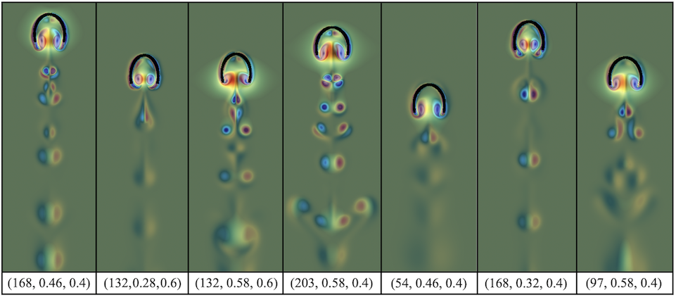
Figure 4: Numerous jellyfish’s vortex wake and position after its $5^{th}$ actuation cycle. Different parameter combinations ($\mathrm{Re},f,p$) led to different swimming behavior, both in terms of distance swam and dynamics, as seen by variations in the vortex wakes left behind. The colormap illustrates fluid vorticity.

The remainder of this section is organized in the following manner. Section 3.1 explores 2D subspaces for all parameter combinations, i.e., $(\mathrm{Re},f)$, $(\mathrm{Re},p)$, and$(f,p)$ for 3 choices of the third input parameter. Section 3.6 provides the results for the global sensitivity analysis using Sobol sensitivity analysis.

3.1 Exploring 2D Parameter Subspaces

Nine total 2D parameter subspaces were explored, each corresponding to a different perpendicular slice from the overall 3D rectangular parameter space, $(\mathrm{Re},f,p)$. Three different cases were performed for each plane:

• $(\mathrm{Re},f)$: $p=0.25,0.50$, and $0.75$

• $(\mathrm{Re},p)$: $f=0.3,0.5$, and $0.7\ \mathrm{Hz}$

• $(f,p)$: $\mathrm{Re}=10,50$, and $250$.

Figure 5 is a summative figure providing data for the three performance metrics of interest - non-dimensional forward swimming speed and cost of transport, as well as Strouhal number in the form of colormaps. The cases illustrated were $(\mathrm{Re},f)$ for $p=0.25$ (top row), $(\mathrm{Re},p)$ for $f=0.3\ \mathrm{Hz}$ (middle row), and $(f,p)$ for $\mathrm{Re}=50$ (bottom row). The colormap values are consistent across every colormap of the same performance metric. From these colormaps parameter regimes in which there is desired swimming performance can be identified. From a quick glance we gathered that non-dimensional swimming speeds $(1/\mathrm{St})$ were maximal for higher $\mathrm{Re}$, lower $f$, and interestingly either lower or higher values of $p$. Values of $p\sim 0.5$ (near the middle of its range) resulted in decreased performance, i.e., lower swimming speed and higher cost of transport. Next we will briefly discuss each 2D parameter subspace separately.

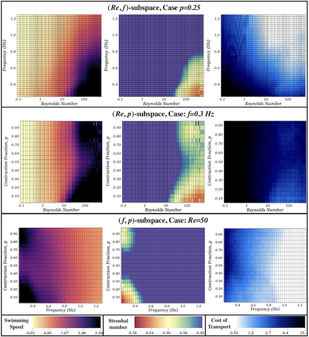
Figure 5: Colormaps illustrating the non-dimensional forward swimming speeds ($1/\mathrm{St}$), Strouhal number ($\mathrm{St}$) and non-dimensional cost of transports ($COT$) over a specific 2D parameter subspace: $(\mathrm{Re},f)$ for the case $p=0.25$ (top row), $(\mathrm{Re},p)$ for the case $f=0.3\ \mathrm{Hz}$ (middle row), and $(f,p)$ for the case of $\mathrm{Re}=50$ (bottom row). Each cell within the colormap represents one particular FSI simulation for the corresponding grid parameter values.

3.2 Discussing the $(\mathrm{Re},f)$-subspace

It has been well established that jet propulsion is an effective technique for forward locomotion in jellyfish for fluid scales of $\mathrm{Re}\gtrsim 10$ Hershlag:2011 ; Yuan:2014 ; Miles:2019b . Figure 6 presents snapshots of overlain independent simulations for a variety of $\mathrm{Re}$, but uniform $f=0.5\ \mathrm{Hz}$ and $p=0.5$. As $\mathrm{Re}$ increases, forward swimming appeared to become increasingly more pronounced, see Figure 7a. Hoover et al. 2015 Hoover:2015 observed that in the case of $\mathrm{Re}=150$ and $p=0.5$ there existed an optimal frequency in which to actuate the bell that resulted in maximal (dimensional) swimming speeds that related to resonant properties of the bell itself. However, it has thus far eluded previous studies to vary both $\mathrm{Re}$ and $f$ in observing swimming performance. Here we explored the subspace of $(\mathrm{Re},f)$ for $3$ different values of $p$, $p=0.25,0.50$, and $0.75$. The data for the subspace corresponding to the case of $p=0.25$ was given in Figure 5.

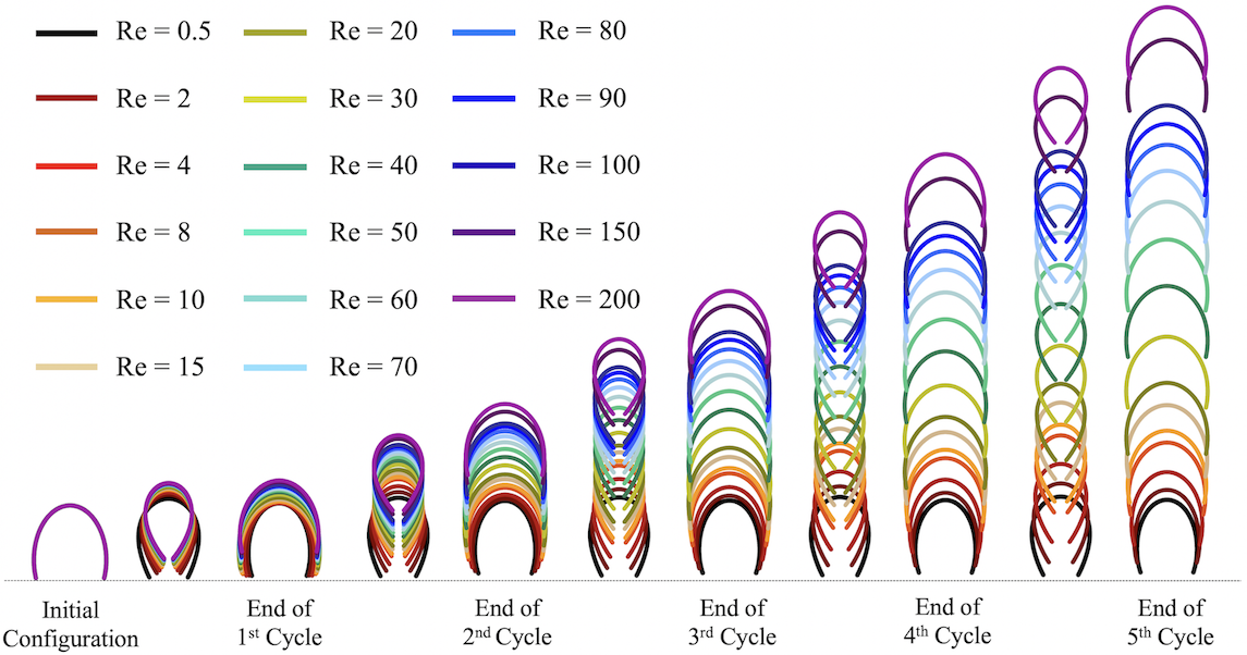
Figure 6: Visualization comparing jellyfish swimming for a variety of $\mathrm{Re}$, all with an actuation frequency of $f=0.5\ \mathrm{Hz}$. Forward swimming is more pronounced for larger $\mathrm{Re}$.

The specific $(\mathrm{Re},f)$ subspace provided in Figure 5 illustrates that forward swimming speeds ($1/\mathrm{St}$) were maximal for $f\lesssim 0.75\ \mathrm{Hz}$ and $\mathrm{Re}\gtrsim 50$. Within that same parameter regime, the Strouhal numbers fell within the biologically relevant regime of $0.2<St<0.4$ Triantafyllou:1991 ; Taylor:2003 ; Floryan:2018 . Although the $COT$ was not minimized across those parameter selections, it did slightly overlap with the region in which $COT$ was near minimized, roughly when $f\approx 0.7$ and $100\lesssim Re\lesssim 250$. Interestingly, those parameter ranges also correspond to the maximum and minimum in the dimensional swimming speed $(V_{dim})$ and dimensional cost of transport $(COT_{dim})$, respectively, see Figures 22 and 23a in Appendix C.4. Overall, the region of lowest cost of transport corresponds to both higher frequency and higher $\mathrm{Re}$, see Figure 7b for a more explicit plot of the data obtained. Figure 7a shows that as $\mathrm{Re}$ increases, swimming speed increased but eventually plateaued.

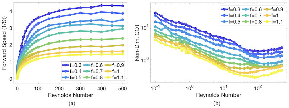
Figure 7: The non-dimensional (a) forward swimming speed and (b) cost of transport as a function of $\mathrm{Re}$ for a variety of different cases involving actuation frequencies, $f$, for $p=0.25$.

Previous jellyfish studies have shown the cost of transport for jellyfish is much lower than other metazoans Gemmell:2013 . However, those studies focused on passive energy recapture in oblate jellyfish, similar to the later computational studies by Hoover et al. 2019 Hoover:2019 , as the main reason for lower COT in comparison. Nonetheless, this analysis so far has shown the existence of optimal parameter combinations in which jellyfish model exhibits maximal forward swimming speed for minimal cost of transport. Although, across the $(\mathrm{Re},f)$-subspace as a whole, the most robust regions for the fastest forward swimming speeds and minimal cost of transports occur over different frequency ranges.

Different 2D slices of the $(\mathrm{Re},f)$-subspace illustrated dependence on contraction fraction, $p$. Recall that lower values of $p$ corresponded to actuation profiles with shorter contraction times and longer expansion times. The region of maximal forward swimming decreased within the space when $p=0.5$, while it grew larger in both the $p=0.25$ and $p=0.75$ case, see Figure 17 in Appendix C.1. Similarly, the size of the region with biologically relevant $\mathrm{St}$ also decreased for $p=0.50$. By comparing minimal values in the $\mathrm{St}$ panels, it was evident that the fastest forward swimming speeds occurred in the case of $p=0.25$. However, this actuation model showed that it is possible to design fast jetting swimmers that have slow contractions but fast expansions, the opposite of how real prolate jellyfish behave Ford:2000 ; Colin:2013 ; Kakani:2013 .

3.3 Discussing the $(\mathrm{Re},p)$-subspace

Previous studies of jellyfish locomotion have established that swimming performance depends on the kinematics of bell actuation Peng:2012 ; Alben:2013 but not how performance may vary across different scales. The middle panels of Figure 5 illustrated that a nonlinear relationship between performance, scale ($\mathrm{Re}$) and the contraction fraction of the overall actuation cycle period, ($p$), across the specific $(\mathrm{Re},p)$ 2D slice corresponding to $f=0.3\ \mathrm{Hz}$. Similar trends in swimming speed ($1/\mathrm{St}$) were observed across $\mathrm{Re}$, such that as $\mathrm{Re}$ increased, speed increased until it eventually began to plateau around $\mathrm{Re}\sim 200-300$ regardless of contraction fraction, $p$, for $f=0.3\ \mathrm{Hz}$, see Figure 18 in Appendix C.2. Figure 7a showed the same trend as $\mathrm{Re}$ increased, but for varying $f$ and only one $p$, $p=0.25$.

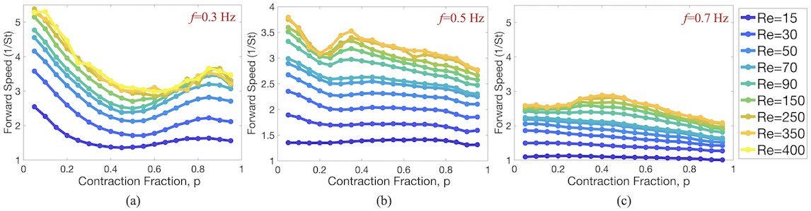
Figure 8: The non-dimensional forward swimming speeds ($1/\mathrm{St}$) as a function $\mathrm{Re}$ for a variety of $p$ for three cases: (a) $f=0.3\ \mathrm{Hz}$, (b) $f=0.5\ \mathrm{Hz}$, and (c) $f=0.7\ \mathrm{Hz}$.

However, as Section 3.2 briefly alluded, swimming performance has a nonlinear relationship with $p$, see Figure 8. For $f=0.3\ \mathrm{Hz}$, both higher and lower values of $p$ resulted in faster forward swimming, while $p$ near the middle of its range ($p\sim 0.5$) resulted in a minimum in swimming speed. This same trend was seen in its dimensional counterpart data, see Figures 22 and 23b in Appendix C.4. As $f$ was increased, different 2D slices showed substantially different behavior. When $f=0.5\ \mathrm{Hz}$, the minimum in speed was found for $p=0.25$. Moreover, speed increased over $0.25\lesssim p\lesssim 0.4$ for $\mathrm{Re}\gtrsim 90$, before beginning to decrease again as $p$ increased. When actuation frequency was set at $f=0.7\ \mathrm{Hz}$ a maximum in forward swimming speed appeared for $p\sim 0.4$ for $\mathrm{Re}\gtrsim 100$. Figure 19 in Appendix C.2 provides colormaps for all 2D slices investigated across the $(\mathrm{Re},p)$-subspace. Although the $COT$ is highest across the 2D slice corresponding to $f=0.3\ \mathrm{Hz}$, as $\mathrm{Re}$ increases, there is an abrupt transition when $\mathrm{Re}\gtrsim 10$ and lower $p$ towards lower $COT$, when compared to all other cases, see Figure 9a. While the $f=0.3\ \mathrm{Hz}$ case resulted in both faster forward swimming and generally higher cost of transport than the other 2D slices that corresponded to higher $f$, the fastest swimming occurred directly over this range of $\mathrm{Re}$ and $p$ in which there was both a sudden drop in and minimal $COT$, but maximal $1/\mathrm{St}$.

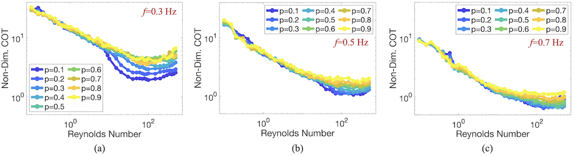
Figure 9: The non-dimensional cost of transport as a function $\mathrm{Re}$ for a variety of $p$ for three cases: (a) $f=0.3\ \mathrm{Hz}$, (b) $f=0.5\ \mathrm{Hz}$, and (c) $f=0.7\ \mathrm{Hz}$.

3.4 Discussing the $(f,p)$-subspace

As the previous two sections have illustrated nonlinear relationships amongst swimming performance and $\mathrm{Re}$ and $f$ or $\mathrm{Re}$ and $p$, here we dove into 2D slices of $(f,p)$-subspace, each corresponding to a different $\mathrm{Re}$. Thus, we focused on changing kinematics of the actuation cycle, both in cycle length (frequency) and contraction versus expansion phase lengths within the overall actuation period. This had not been previously studied for jellyfish or other organisms that swim via jet propulsion. The bottom panels of Figure 5 give the performance data for the 2D slice corresponding to $(f,p)$ and $\mathrm{Re}=50$.

Lower $f$ ($f\lesssim 0.4\ \mathrm{Hz}$) and either low or high values or $p$ ($p<0.3$ or $p>0.7$) resulted in higher swimming speeds, see the bottom panels in Figure 5, corresponding to $(f,p)$ for $\mathrm{Re}=50$. These regions also displayed $\mathrm{St}$ within the biologically relevant range. From minimal values in the $\mathrm{St}$ panel, it was observed that the fastest swimmers over this 2D slice were the ones in which contracted their bells the quickest, i.e., smaller values of $p$. Moreover, this region $(p\lesssim 0.3)$ also corresponded to a lower $COT$ than the other region in which produced faster jellyfish, i.e., $p>0.6$. However, the minimal region for $COT$ occurred for $f\gtrsim 1.0\ \mathrm{Hz}$ regardless of $p$. As $f$ increased, the swimming speeds converged across multiple of $p$, as Figures 21 and 20a in Appendix C.3 indicated.

Figure 21 provides the data for the other 2D slices explored for cases of $(f,p)$ and $\mathrm{Re}=10,50$, and $250$. As $\mathrm{Re}$ increased, the size of the region in which there were maximal swimming speeds increased, across both $f$ and $p$ directions. However, as the smaller values in the $\mathrm{St}$ panel indicated, the fastest jellyfish were produced for smaller values of $p$.

The dimensional form of the data shows the existence of two optimal frequencies to in which to actuate the bell for lower values of $p$, see Figure 23c in Appendix C.4. Hoover et al. 2015 uncovered one of these such frequencies when they showed the existence of an optimum frequency in which to actuate the bell for the specific case of $p=0.50$. That frequency corresponded to the resonant frequency in which to actuate the jellyfish bell to gain a boost in forward swimming speed. Here it corresponded to the frequency of $f\sim 0.75\ \mathrm{Hz}$. Interestingly, our data showed that the emergence of another notable frequency when $p\lesssim 0.3$ that appeared to be half that resonant frequency value, $f\sim 0.375\ \mathrm{Hz}$. The dimensional data for $\mathrm{St}$ and $COT$ are provided in Figure 22 in Appendix C.4 as well for the case of $\mathrm{Re}=50$ across the $(f,p)$-subspace.

3.5 Exploring COT vs. Forward Swimming Speed

A Pareto-like front was observed when the non-dimensional cost of transport ($COT$) and the non-dimensional swimming speed ($1/\mathrm{St}$) were plotted against each other Eloy:2013 ; Verma:2017 ; Schuech:2019 ; Smits:2019 , see Figure 10a. We deemed these Pareto-like since optimal parameter combinations for locomotion would be those in which resulted in maximal swimming speeds for minimal cost of transport, rather than maximal values in both quantities, as how traditional Pareto optimization strategies are constructed. Figure 10a displays the combination of all the data from Sections 3.2-3.4. $COT$ was minimal in cases of parameter combinations that resulted in a jellyfish’s forward swimming speed of $1/St\sim 1$. For different swimming speeds along the curve of minimal $COT$, when speeds decreased from $1$, the $COT$ increased rapidly. For speeds slightly larger than $1$ on the curve of minimal $COT$, there was a sharp increase in $COT$. However, when speeds further increased away from $1$, $COT$ increased much more slowly. As speed increased along the minimal curve from $2$ to $5$, the cost of transport only increased approximately from $0.5$ to $1.0$.

By probing further into where individual subspaces lied within the overall performance space, patterns emerged, see Figures 10b-d. For the $(\mathrm{Re},f)$-subspaces, each corresponding to a different $p$, the data mostly all overlapped, see Figure 10b. That is, given a $p$, different combinations of $(\mathrm{Re},f)$ could almost fill out the entire performance space. A quick glance of the $(\mathrm{Re},p)$ and $(f,p)$-subspaces told a different story. On the $(\mathrm{Re},p)$-subspaces, different values of $f$ placed all $(\mathrm{Re},p)$ combinations into particular regions within the performance space. Higher $f$ corresponded to lower $COT$ for all $3$ slices considered. Although, as $f$ increased, the maximum attainable swimming speeds decreased. Each cluster corresponding to a different $f$ aligned more closely with swimming speed, i.e., along each cluster as speeds increased, the $COT$ did not substantially change. The $(f,p)$-subspaces illustrated that for a given $\mathrm{Re}$, different combinations of $(f,p)$ could result in low or high swimming speeds, with either lower or higher or cost of transports. Smaller $\mathrm{Re}$ had a much more pronounced vertical presence within the performance space, i.e., for the $\mathrm{Re}=10$ case, swimming speeds did not substantially change within the cluster when compared to the higher $\mathrm{Re}$ cases, although its cost of transport substantially varied across the subspace. The analog involving dimensional data for the cost of transport and swimming speeds showed similar clustering trends; the $(\mathrm{Re},f)$-subspace slices all seemed to overlap, while the different cases for the $(\mathrm{Re},p)$ and $(f,p)$-subspaces appeared to cluster more into particular regions within the performance space, see Figure 24 in Appendix C.4.

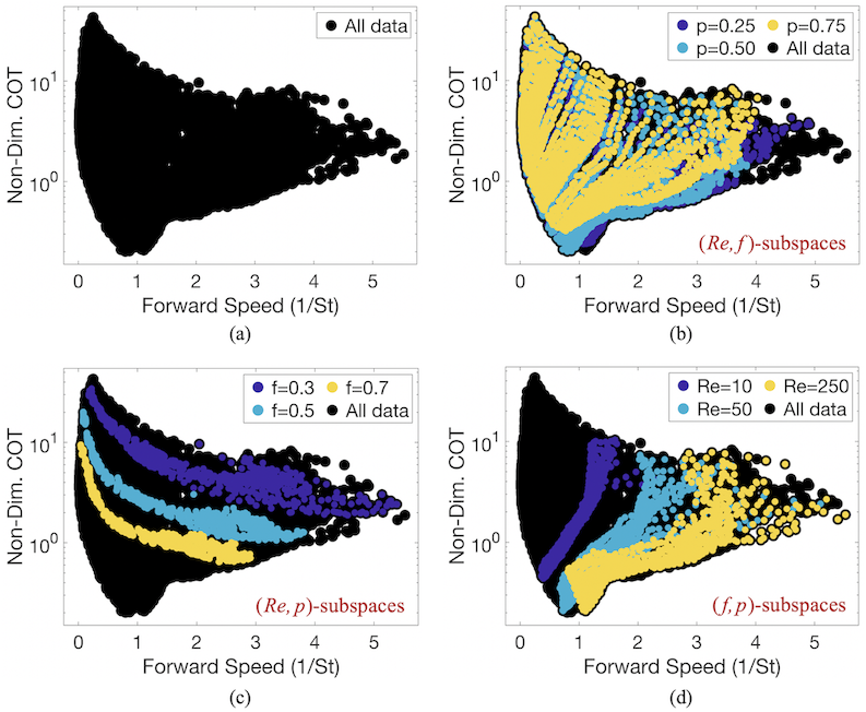
Figure 10: The non-dimensional average cost of transports and forward swimming speeds ($1/\mathrm{St}$) plotted against each other. (a) Data from all simulations, as well as highlighted regions within the performance spaces corresponding to different ranges of the input parameters: (b) different $\mathrm{Re}$ (c) different $f$, and (d) different $p$.

3.6 Global Sensitivity Analysis

The jellyfish model’s global sensitivity to $(\mathrm{Re},p,f)$ was assessed with Sobol sensitivity analysis. The sensitivity analysis was conducted over the a space in which resulted in substantial forward swimming, i.e., $\mathrm{Re}\times f\times p=[50,250]\times[0.3,1.25]\times[0.05,0.95].$ The $\mathrm{Re}$ were chosen due to the increases in swimming speed observed over this range, before swimming speed ultimately plateaued, see Figures 7 and 18. The range of $f$ was selected because it centered around the resonant frequency peak of $\sim 0.75\ \mathrm{Hz}$ (see Section 3.4), included lower values of $f$, which resulted in maximal non-dimensional swimming speeds (see Sections 3.2-3.4, as well as frequencies slightly larger than that of the jellyfish like Sarsia tubulosa Colin:2013 but below that of Catostylus mosaicus Neil:2018b . Recall that although Catostylus mosaicus has a fineness ratio of $\sim 1$, its morphology is much more complex, as it includes dense oral arms and an intricate tentacle structure. Thus we decided to keep frequencies within a range for jellyfish without much complex tentacle or oral arm structure, like Sarsia tubulosa Kakani:2013 ; Katija:2015b . While it is known that real prolate jellyfish exhibit much shorter contraction phases than expansion phases Ford:2000 ; Colin:2013 ; Kakani:2013 , we elected to study the complete range of $p$ from $0.05<p0.95$ since effective swimming was observed for both ends of the range (see Section 3.4).

As mentioned previously, 5000 parameter combinations were sampled within this parameter space, via Sobol sequencing. Each sampled parameter combination was then simulated in order to perform Sobol sensitivty analysis on the desired swimming performance metrics - swimming speed, Strouhal number, and cost of transport. Once they were computed, the Sobol sensitivity indices were calculated Sobol:2001 ; Saltelli:2010 .

Figure 11 provides the indices for both the first-order and total-order parameter interactions that were found. Within the restricted parameter space, the swimming performance metrics were most sensitive to variations in actuation (stroke) frequency, $f$. Some higher-order interactions between the parameter exist, as the first-order indices and total-order indices are not equivalent, particularly when comparing the first and total-order indices related to $p$. However, both the first and total-order indices indicated the performance metrics were most sensitive to $f$. This was consistent even for the dimensional analogs of swimming speed and cost of transport. Moreover, the degree of sensitivity to each parameter varied across all performance metrics. Note that while we only varied $\mathrm{Re},f$, and $p$, it is possible that the efficiency metrics could be more sensitive to other parameters that were not explored here, such as different material properties, i.e., bell stiffnesses Hoover:2015 ; Hoover:2019 , duration of inactive (gliding) phases of swimming Videler:1982 ; Peng:2012 ; Alben:2013 , contraction force strength Hoover:2015 ; Hoover:2017 ; Hoover:2019 , or especially the fineness ratio Peng:2012 , which appears to dictate a jellyfish’s main mode of locomotion, either a jet propulsion or jet-padding mode Ford:2000 ; Colin:2002 ; Costello:2008 ; Weston:2009 .

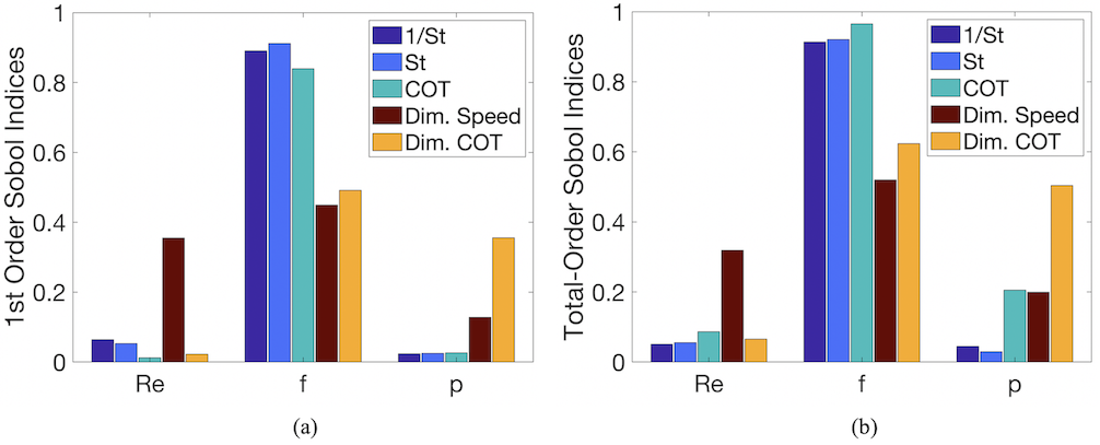
Figure 11: (a) First-order and (b) Total-order Sobol indices corresponding to 3 swimming performance metrics: non-dimensional swimming speed ($1/\mathrm{St}$), Strouhal number ($\mathrm{St}$), non-dimensional cost of transport ($COT$), for the three input parameters: $\mathrm{Re}$, $f$, and $p$.

The Sobol sensitivity analysis alone granted us sensitivity indices for each parameter; however, it did not divulge in what way the performance metrics were sensitive to each parameter. For example, if $f$ was increased from one value to another, it was unclear whether swimming speeds would increase or decrease. To explore these effects, the entire parameter space sampled via Sobol sequences was projected into three distinct subspaces: $(\mathrm{Re},f)$, $(\mathrm{Re},p)$, and $(f,p)$, as illustrated by the process in Figures 12b-c. Having performed 5000 simulations, the resulting projected subspaces appeared “filled”. We then observed trends within each projected subspace.

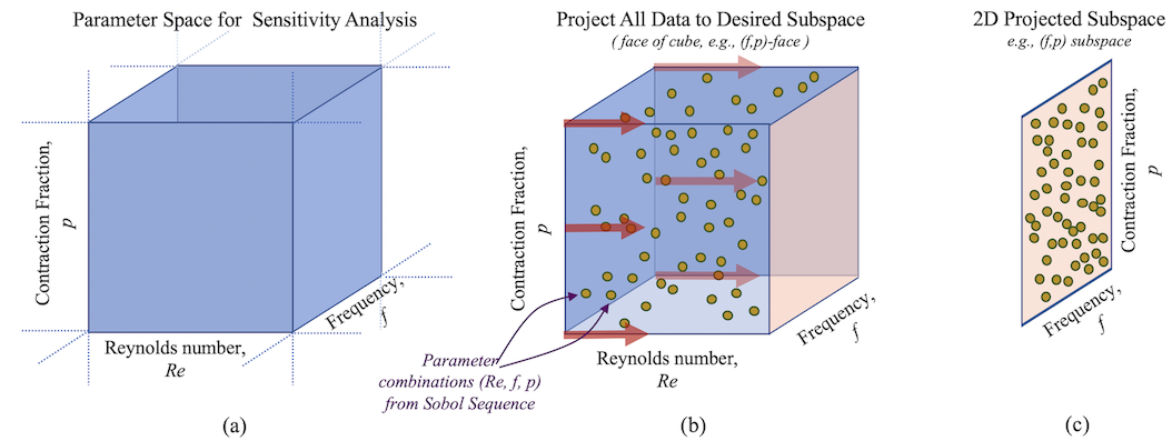
Figure 12: (a) The overall $3D$ parameter space being sampled by Sobol sequences. (b) Illustration of sampling points via Sobol sequences being projected into a $2D$ subspace, here the $(f,p)$ subspace (c) Visualization of where data is projected from a higher dimension space into a $2D$ subspace. Figure adapted courtesy of Battista:ICB2020b .

Figure 13 provides the performance data across each projected subspace. The gradients in color provided a mechanism to observe emergent patterns within each projected subspace. Qualitatively, across the $(\mathrm{Re},f)$ and $(f,p)$-projected subspaces, the gradient fronts mostly corresponded with variations in $f$. For a given $f$ in these subspaces, some slight dependence was observed on the other parameter, either $\mathrm{Re}$ or $p$, respectively, as the gradient fronts were not completely horizontal in the $(\mathrm{Re},f)$-projected subspaces or vertical in $(f,p)$-projected subspaces. On the other hand, no discernible pattern emerged for any performance metrics within the $(\mathrm{Re},p$)-projected subspace. Thus, qualitative patterns were only noticeable when $f$ was varied, the parameter to whom the model was most sensitive to. Moreover, the most significant variations in these projected subspaces across each performance metric were in the direction of varying $f$. The dimensional analog to Figure 13 is provided in Figure 25 in Appendix C.4.

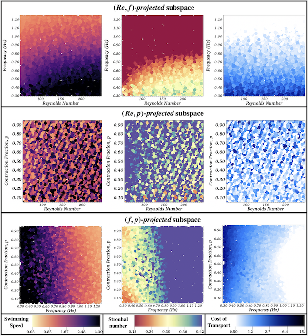
Figure 13: Colormaps of the projected data across all 5000 sampled parameter cases from the Sobol sequence giving the non-dimensional forward swimming speeds ($1/\mathrm{St}$) and cost of transports ($COT$) onto either the $(\mathrm{Re},f)$, $(\mathrm{Re},p)$, or $(f,p)$ subspace.

Similar to the analysis in Section 3.5, a Pareto-like front was observed by plotting the non-dimensional cost of transport ($COT$) against the non-dimensional swimming speed ($1/\mathrm{St}$) Eloy:2013 ; Verma:2017 ; Schuech:2019 ; Smits:2019 , see Figure 14a. Figures 14b-d, depict how different input parameter ranges fall within the performance space for all the simulations performed for the Sobol sensitivity analysis. Figures 14b and 14d show that for a given $\mathrm{Re}$ or $p$, respectively, that different combinations of the other two input parameters, $(f,p)$ or $(\mathrm{Re},f)$, respectively, could produce a jellyfish whose performance could span the entire performance space. However, different $f$ cluster the performance data into distinct regions within the performance space, see Figure 14b. Higher $f$ pushed the cluster towards both lower swimming speeds and lower cost of transport. This further supported that the notion that this jellyfish model’s performance output was most sensitive to the actuation frequency, $f$.

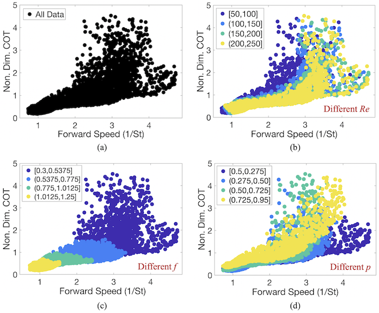
Figure 14: The non-dimensional average cost of transports and forward swimming speeds ($1/\mathrm{St}$) plotted against each other of the data from the Sobol analysis. (a) All data from Sobol simulations, as well as highlighted regions within the performance spaces corresponding to different ranges of the input parameters: (b) different $\mathrm{Re}$ (c) different $f$, and (d) different $p$.

4 Discussion and Conclusion

Experimental studies of jellyfish locomotion have previously found that not only does bell morphology and scale affect swimming performance Colin:2002 ; Dabiri:2005b ; Costello:2008 but also the bell kinematics itself Dabiri:2006 ; Gemmell:2015 . Here we demonstrated through a 2D fluid-structure interaction model of jellyfish forward locomotion how complex the relationship between scale ($\mathrm{Re}$) and bell kinematics, including actuation frequency ($f$) and the contraction phase percentage of the overall actuation cycle ($p$), is on its achievable swimming performance. Two-dimensional CFD models of jet propulsive prolate jellyfish models have previously shown both qualitative and quantitative agreement with experiments Sahin:2009b ; Hershlag:2011 ; Alben:2013 ; Kakani:2013 . Our model recreated similar swimming performance profiles of previous jellyfish locomotion computational models Hershlag:2011 ; Alben:2013 ; Yuan:2014 ; Hoover:2015 . Notably, we saw similar trends in which forward swimming speed plateaued when $\mathrm{Re}$ was high enough Hershlag:2011 ; Miles:2019b ; however, we also determined that this trend was conserved across all contraction frequencies and contraction phase percentages (see Figures 7 and 18).

Non-linear relationships arose between the three input parameters $(\mathrm{Re},f,p)$ in which could maximize (or minimize) non-dimensional forward swimming speed ($1/St$) and cost of transport ($COT$) across different 2D slices within the 3D parameter space. Jellyfish with faster contraction times generally resulted in faster forward swimming speeds Peng:2012 ; Alben:2013 ; however, as Figures 5, 8, 19, and 23c illustrated, given a $f$, maxima in $1/St$ occur for different ranges of $p$. Therefore our model showed that it is not always true that faster swimming results when the contraction time is faster than the expansion time, i.e., $p<0.5$. It also depends on both frequency and scale. Faster contraction times also led to decreased cost of transport within the $\mathrm{Re}$ regimes that also resulted in pronounced swimming, see Figure 9. Peng and Alben 2012 Peng:2012 had suggested the opposite relationship previously. Furthermore, substantial swimming speeds were also observed for faster expansions than contractions, i.e., $p>0.5$, but these cases also resulted in higher cost of transports. For $\mathrm{Re}>50$, lower $f$ generally resulted in faster forward swimming behavior, see Figures 5 and 17. For $\mathrm{Re}\gtrsim 30$ and a given $p$, an optimal frequency emerged in which resulted in maximized forward swimming in the dimensional speed data, see Figures 22 and 23, as in Hoover et al. 2015 Hoover:2015 . The idea of driving jellyfish bells at resonance dates back to 1988 in which the work of Demont and Gosline Demont:1998c showed remarkable benefits in both energetic costs and forward propulsion in the prolate jellyfish Polyorchis penicillatus. Moreover, a second notable frequency emerged in Figures 23a and 23c, which maximized forward swimming speed when $\mathrm{Re}\gtrsim 30$ and $p\lesssim 0.3$. This second frequency appeared to be roughly half that of the optimal (resonant) frequency and also corresponded to minimal cost of transports, see Figure 22. This second frequency had not been documented previously.

While prolate jellyfish exhibit higher cost of transports than oblate jellyfish Dabiri:2007 ; Dabiri:2010b , which deem them as less efficient swimmers, it is not due to their swimming speeds. They achieve must faster forward swimming speeds but through a more energetically expensive jet propulsive mode of locomotion. Many juvenile jellyfish exhibit jet propulsive modes, due to their higher fineness ratios ($\sim>1$) during development McHenry:2003 ; Weston:2009 ; Blough:2011 . Due to evolutionary constraints of the musculature thickness of cnidarians, the jet propulsive technique becomes ineffective for prolate jellyfish much larger than 10cm Dabiri:2007 ; Costello:2008 ; Colin:2013 . Thus, as they continue to grow and develop, their bell morphologies change to more oblate shapes (lower fineness ratios), which changes their locomotive mode as an adult to rowing or jet-paddling Weston:2009 ; Blough:2011 . Theoretical limits for jet propulsion at the interface between oblate and prolate jellyfish were found, see the performance space Figures 10 and 14 plotting cost of transport against swimming speed. Clusters within these performance spaces emerged for $\mathrm{Re}$ and $f$ (Figure 10) or $f$ (Figure 14), to which the latter involved a restricted parameter input space that resulted in greater swimming performance. Furthermore, Pareto-like optimal fronts were attained through this analysis. That is, for a given desired swimming speed within the performance space, parameter combinations could be found in which resulted in the minimal cost of transport.

Global sensitivity analysis showed that the performance metrics were most sensitive to actuation (stroke) frequency across an input parameter space which yield substantial forward swimming behavior, whether in dimensional or non-dimensional units, see Figure 11. Although jellyfish swimming performance was known to be dependent on stroke frequency Peng:2012 ; Hoover:2015 , the Sobol sensitivity analysis quantitatively suggested that for a jellyfish whose fineness ratio is 1 and that uses a jet propulsive locomotion mode, its swimming performance is most affected by stroke frequency. A computational study examining an anguilliform mode of locomotion in nematodes also found that their locomotion mode was most affected by variations in stroke frequency Battista:ICB2020b . These analyses were both conducted over a parameter space of high swimming performance, which here included $\mathrm{Re}>50$. Therefore, additional studies are warranted to explore global sensitivity at lower $\mathrm{Re}$, which would include either juvenile Gordon:2017 or smaller jellyfish Kakani:2013 . Furthermore, for jellyfish in general, it is not clear how their performance metrics’ global sensitivity could change if other input parameters were varied or incorporated, such as the bell’s material properties and morphology Colin:2002 ; Dabiri:2007 ; Hoover:2015 ; Katija:2015 ; Hoover:2019 ; Miles:2019b , contraction kinematics, i.e., jetting or jet-paddling modes Colin:2002 ; Dabiri:2007 or gliding times between successive strokes Videler:1982 ; Peng:2012 ; Alben:2013 , contraction strength Hoover:2015 ; Hoover:2017 ; Hoover:2019 , fineness ratio Peng:2012 .

Introducing more uncertain model input parameters, such as those quantities suggested above, would have exponentially increased the number of required simulations for the Sobol sensitivity analysis, and hence also the computational expense Nossent:2011 . Here 5000 simulations were explicitly performed for the sensitivity analysis in order for the Sobol sensitivity indices to converge. These simulations required approximately 360,000 computational hours. Thus, using traditional Sobol sensitivity analysis through the formation of a Sobol sequence is not scalable for fluid-structure interaction models exploring high dimensional input spaces ($>3$). Recently, contemporary methods involving polynomial chaos have emerged as a plausible alternative, as they require far fewer simulations in order for the sensitivity indices to converge Xiu:2003 ; Xiu:2003b ; Sudret:2008 ; Waldrop:2018 ; Waldrop:ICB2020 ; Waldrop:JRS2020 . Thus they heavily reduce the computational burden; however, by significantly reducing the number of simulations performed may also prohibit the possibility of resolving projected parameter subspaces, like those in Figures 13 and 25. Thereby, while the performance output’s global sensitivity would be quantified, it could remain unclear how performance itself varied across the higher dimensional input parameter space.

Appendix A Details on IB

A two-dimensional formulation of the immersed boundary (IB) method is discussed below. The open-source IB software, IB2d, was used to perform all fluid-structure interaction simulations Battista:2015 ; BattistaIB2d:2017 ; BattistaIB2d:2018 . The software itself has been validated BattistaIB2d:2017 and specific grid resolution convergence tests pertaining to this jellyfish model were also performed previously BattistaMizuhara:2019 . Additional domain size convergence tests were also performed, with details given below in Appendix B. For a full review of the immersed boundary method, please see Peskin 2002 Peskin:2002 or Mittal et al. 2005 Mittal:2005 .

A.1 Governing Equations of IB

The conservation of momentum and mass equations that govern an incompressible and viscous fluid are listed below:

$$\rho\Big{[}\frac{\partial{{\bf u}}}{\partial t}({\bf x},t)+{{\bf u}}({\bf x},t)\cdot\nabla{{\bf u}}({\bf x},t)\Big{]}=-\nabla p({\bf x},t)+\mu\Delta{{\bf u}}({\bf x},t)+{{\bf f}}({\bf x},t)$$ (11)

$${\nabla\cdot}{{\bf u}}({\bf x},t)=0$$ (12)

where ${{\bf u}}({\bf x},t)$ is the fluid velocity, $p({\bf x},t)$ is the pressure, ${{\bf f}}({\bf x},t)$ is the force per unit area applied to the fluid by the immersed boundary, $\rho$ and $\mu$ are the fluid’s density and dynamic viscosity, respectively. The independent variables are the time $t$ and the position ${\bf x}$. The variables ${{\bf u}},p$, and ${{\bf f}}$ are all written in an Eulerian frame on the fixed Cartesian mesh, x.

The interaction equations, which handle all communication between the fluid (Eulerian) grid and immersed boundary (Lagrangian grid) are the following two integral equations:

$${\bf f}({\bf x},t) =\int{\bf F}(s,t)\delta\left({\bf x}-{\bf X}(s,t)\right)ds$$ (13)

$${\bf U}({\bf X}(s,t)) =\int{{\bf u}}({\bf x},t)\delta\left({\bf x}-{\bf X}(s,t)\right)d{\bf x}$$ (14)

where ${\bf F}(s,t)$ is the force per unit length applied by the boundary to the fluid as a function of Lagrangian position, $s$, and time, $t$, $\delta({\bf x})$ is a two-dimensional delta function, and ${\bf X}(s,t)$ and ${\bf U}(s,t)$ give the Cartesian coordinates and velocity at time $t$ of the material point labeled by the Lagrangian parameter, $s$, respectively. The Lagrangian forcing term, ${\bf F}(s,t)$, gives the deformation forces along the boundary at the Lagrangian parameter, $s$. Equation (13) applies this force from the immersed boundary to the fluid through the external forcing term in Equation (11). Equation (14) moves the boundary at the local fluid velocity. This enforces the no-slip condition. Each integral transformation uses a two-dimensional Dirac delta function kernel, $\delta$, to convert Lagrangian variables to Eulerian variables and vice versa.

Using delta functions as the kernel in Eqs.(13-14) is what gives IB its power. To approximate these integrals, discretized (and regularized) delta functions are used. We use the ones given from Peskin:2002 , i.e., $\delta_{h}(\mathbf{x})$,

$$\delta_{h}(\mathbf{x})=\frac{1}{h^{3}}\phi\left(\frac{x}{h}\right)\phi\left(\frac{y}{h}\right)\phi\left(\frac{z}{h}\right),$$ (15)

where $\phi(r)$ is defined as

$$\phi(r)=\left\{\begin{array}[]{l}\frac{1}{8}(3-2|r|+\sqrt{1+4|r|-4r^{2}}),\ \ \ \ \ 0\leq|r|<1\\ \frac{1}{8}(5-2|r|+\sqrt{-7+12|r|-4r^{2}}),\ 1\leq|r|<2\\ 0\hskip 123.58218pt2\leq|r|.\\ \end{array}\right.$$ (16)

A.2 Numerical Algorithm

As stated in the main text, we imposed periodic and no slip boundary conditions on the rectangular domain. To solve Equations (11), (12),(13) and (14) we needed to update the fluid’s velocity and pressure as well as the position of the boundary and force acting on the boundary at time $n+1$ using data from time $n$. The IB does this in the following steps Peskin:2002 .

Step 1: Find the force density, ${\bf{F}}^{n}$ on the immersed boundary, from the current boundary configuration, ${\bf{X}}^{n}$.
Step 2: Use Equation (13) to spread this boundary force from the Lagrangian boundary mesh to the Eulerian fluid lattice points.
Step 3: Solve the Navier-Stokes equations, Equations (11) and (12), on the Eulerian grid. Upon doing so, we are updating ${\bf{u}}^{n+1}$ and $p^{n+1}$ from ${\bf{u}}^{n}$, $p^{n}$, and ${\bf{f}}^{n}$.
Step 4: Update the material positions, ${\bf{X}}^{n+1}$, using the local fluid velocities, ${\bf{U}}^{n+1}$, computed from ${\bf{u}}^{n+1}$ and Equation (14).

Appendix B Computational Grid Width Convergence Check

A convergence test was performed to determine how the width of the computational domain, $L_{x}$, affected forward swimming speeds and vortex wake topology. We investigated cases for $Re=\{37.5,75,150,300\}$ and computed forward swimming speed and the subsequent error between cases of different widths of $L_{x}=\{3,3.5,4,\ldots,8\}$. The height of the domain was fixed with $L_{y}=12$ and spatial step-sizes was conserved in every computational domain case, i.e., $dx=dy$.

Figure 15a and b provides the swimming speed for every $L_{x}$ and $\mathrm{Re}$ considered and relative error between each case of $L_{x}$ against the widest case of $L_{x}$, respectively. Figure 15a showed that for every case of $\mathrm{Re}$ considered, thinner width simulations produced slightly slower swimming jellyfish; however, the differences in speed were small. As the width gets larger, the relative error decreases, as illustrated by Figure 15b. Moreover, when $L_{x}=3$, the relative error percentage was $\sim 5.5-6.5\%$ and by $L_{x}=5$, the relative error decreased to $\sim 1-1.5\%$. We chose to run simulations using $L_{x}=5$ in an attempt to minimize computational cost while preserving adequate accuracy.

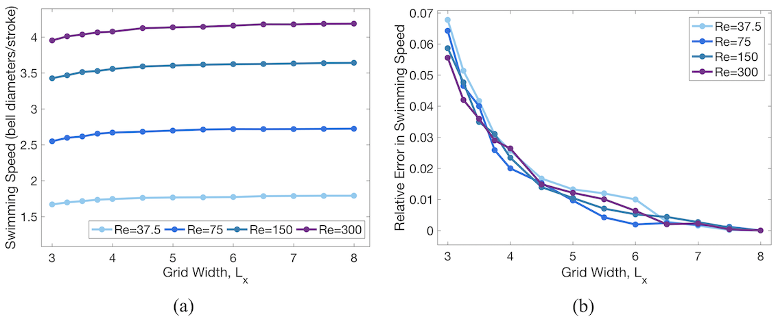
Figure 15: $ConvergenceCheck$: $Re=150$ for different computational mesh widths.

Furthermore, Figure 16 illustrated that qualitative differences were negligible in vortex wake topology in the case of $(\mathrm{Re},f,p)=(150,0.65,0.5)$ across the $4^{th}$ to $5^{th}$ actuation cycle. Cases involving other parameter combinations followed similarly. Subtle differences in vortex dynamics are only observed in down stream vortices when $L_{x}>5$.

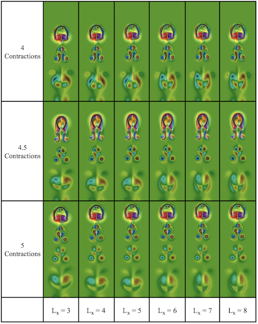
Figure 16: Convergence check for the case with $(\mathrm{Re},f,p)=(150,0.65,0.5)$ with differing widths of the computational domain, $L_{x}$.

Appendix C Additional Simulation Data

Additional simulation data is provided below. This data complements those presented in the main text of the manuscript. This section is divided into the following sections:

• C.1: Data complementing the $(\mathrm{Re},f)$-subspace explorations from Section 3.2

• C.2: Data complementing the $(\mathrm{Re},p)$-subspace explorations from Section 3.3

• C.3: Data complementing the $(f,p)$-subspace explorations from Section 3.4

• C.4: Swimming performance data in dimensional units complementing the non-dimensional data presented in Sections 3.1-3.6.

C.1 Additional data for the $(\mathrm{Re},f)$-subspace

The data corresponding to all 2D slices of the $(\mathrm{Re},f)$ is presented in Figure 17. The three cases given correspond to the $(\mathrm{Re},f)$-subspace for $p=0.25$ (top row), $p=0.50$ (middle row), and $p=0.75$ (bottom row) in the figure. Variations in the topography of the performance landscapes were minimal across different 2D slices. That is, the sizes of the regions with minimal or maximal performance slightly varied with $p$, but the overall structure remained consistent.

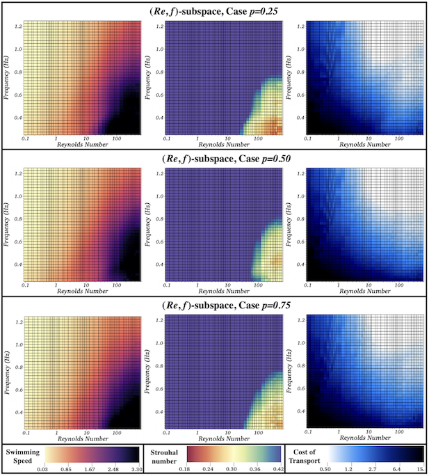
Figure 17: Colormaps corresponding to all cases investigated for the $(\mathrm{Re},f)$-subspace for $p=0.25$ (top row), $p=0.50$ (middle row), and $p=0.75$ (bottom row). Each cell within the colormap represents one particular FSI simulation for the corresponding grid parameter values.

C.2 Additional data for the $(\mathrm{Re},p)$-subspace

The average non-dimensional forward swimming speeds ($1/\mathrm{St}$) and cost of transports as a function of $\mathrm{Re}$ are provided in Figure 18, for a variety of different contraction fractions, $p$, and frequency, $f=0.5\ \mathrm{Hz}.$ Faster contraction times (smaller $p$) appeared to correspond to faster jellyfish swimming speeds and lower cost of transports as $\mathrm{Re}$ increased. For $Re\lesssim 10$, both swimming speed and cost of transport did not substantially vary for different $p$.

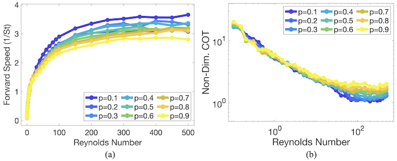
Figure 18: The average non-dimensional (a) forward swimming speed and (b) cost of transport as a function of $\mathrm{Re}$ for a variety of different cases involving contraction fractions, $p$, for the case of $f=0.5\ \mathrm{Hz}$.

The data corresponding to all 2D slices of the $(\mathrm{Re},p)$-subspace are given in Figure 19. The three cases shown correspond to the $(\mathrm{Re},p)$-subspace for $f=0.3\ \mathrm{Hz}$ (top row), $f=0.5\ \mathrm{Hz}$ (middle row), and $f=0.7\ \mathrm{Hz}$ (bottom row) in the figure. As $f$ varied, there were substantial differences in the topography of each performance landscape. Generally, as $f$ increased the size of the region corresponding to maximal forward swimming speeds decreased, while the region for minimal cost of transport increased in each successive landscape.

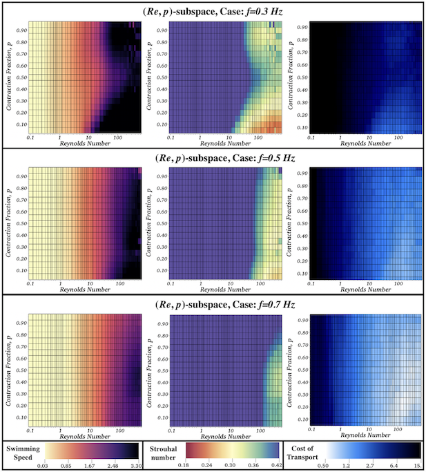
Figure 19: Colormaps corresponding to all cases investigated for the $(\mathrm{Re},p)$-subspace for $f=0.3\ \mathrm{Hz}$ (top row), $f=0.5\ \mathrm{Hz}$ (middle row), and $f=0.7\ \mathrm{Hz}$ (bottom row). Each cell within the colormap represents one particular FSI simulation for the corresponding grid parameter values.

C.3 Additional data for the $(f,p)$-subspace

The average non-dimensional forward swimming speeds ($1/\mathrm{St}$) and cost of transports as a function of $f$ for a variety of $p$ and $p$ for a variety of $f$ are provided in Figures 20a and 20b, respectively, for the case of $Re=50$. Swimming speeds all converged for higher frequencies, regardless of contraction fraction, $p$. However, for smaller $f$, minimal values in swimming speed arose for $p\sim 0.5.$ Higher cost of transport was associated with smaller frequencies, see Figure 20c. Moreover, faster contraction times (smaller $p$) resulted in decreased cost of transport.

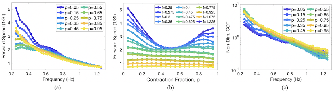
Figure 20: The average non-dimensional swimming speed as (a) a function $f$ for a variety of $p$ and (b) a function of $p$ for a variety of $f$ as well as (c) the non-dimensional cost of transport as a function of $f$ for a variety of $p$.

The data corresponding to all 2D slices of the $(f,p)$-subspace are given in Figure 21. The three cases shown correspond to the $(\mathrm{Re},p)$-subspace for $Re=10$ (top row), $Re=50$ (middle row), and $Re=250$ (bottom row) in the figure. As $\mathrm{Re}$ varied, there were substantial differences in the topography of each performance landscape. Generally, as $\mathrm{Re}$ increased the size of the regions corresponding to maximal forward swimming speeds and minimal cost of transport both increased in each successive landscape. However, these regions did not overlap for any $\mathrm{Re}$ case.

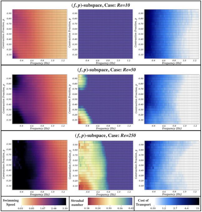
Figure 21: Colormaps corresponding to all cases investigated for the $(f,p)$-subspace for $Re=10$ (top row), $Re=50$ (middle row), and $Re=250$ (bottom row). Each cell within the colormap represents one particular FSI simulation for the corresponding grid parameter values.

C.4 Swimming Performance Data in Dimensional Units

The dimensional data that complements Figure 5 is provided in Figure 22. The 2D slice corresponding to the $(\mathrm{Re},f)$-subspace for $p=0.25$ showed the existence of a robust region of maximal swimming speeds for $f\sim 0.7\ \mathrm{Hz}$ and $Re\gtrsim 100$. Similarly, the $(\mathrm{Re},p)$-subspace for $f=0.3\ \mathrm{Hz}$ showed maximal swimming speeds for $Re\gtrsim 50$ and either low $p$ (fast contraction times) or high $p$ (slow contraction times). Minimal swimming speeds occurred when contraction and expansion times were approximately equal ($p\sim 0.5$). The $(f,p)$-subspace for $Re=50$ divulged maximal swimming speed clusters around $f\sim 0.35\ \mathrm{Hz}$ and $f\sim 0.7\ \mathrm{Hz}$ for faster contraction times ($p\lesssim 0.2$). However, other substantially fast regions appeared over different $(f,p)$ ranges, e.g., $0.6\gtrsim f\gtrsim 0.8$ and $0.20\gtrsim p\gtrsim 0.70$. Lower costs of the transport were generally observed in the $(\mathrm{Re},f)$- and $(\mathrm{Re},p)$-subspaces as $\mathrm{Re}$ increased. In those subspaces for $Re\gtrsim 50$, nonlinear dependence on $f$ and $p$, respectively, led to regions of minimal cost of transport. The $(f,p)$-subspace illustrated distinct parameter clusters in which led to minimal cost of transport. The region encasing $p\lesssim 0.2$ and $0.3\gtrsim f\gtrsim 0.4$ had some of the fastest swimming speeds and lowest costs of transport within the subspace.

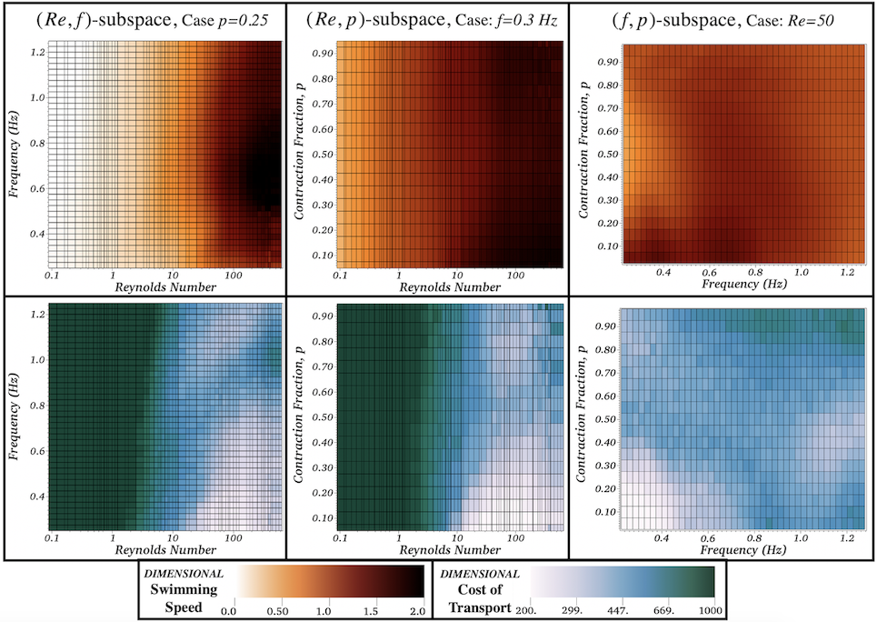
Figure 22: Colormaps illustrating the dimensional forward swimming speed ($V_{dim}$) and cost of transport ($COT_{dim}$) to complement the non-dimensional performance data from Figure 5 in Section 3.1. Performance data is represented across 2D parameter subspace: $(\mathrm{Re},f)$ for the case $p=0.25$ (left column), $(\mathrm{Re},p)$ for the case $f=0.3\ \mathrm{Hz}$ (middle column), and $(f,p)$ for the case of $Re=50$ (right column). Each cell within the colormap represents one particular FSI simulation for the corresponding grid parameter values.

Explicit plots of the data complementing the colormaps in Figure 22 are provided in Figure 23. Nonlinear relationships emerged across every 2D subspace explored. The optimal actuation frequency found in Figure 23a for the case of $Re=150$ agreed with the resonant frequency analysis from Hoover et al. 2015 Hoover:2015 .

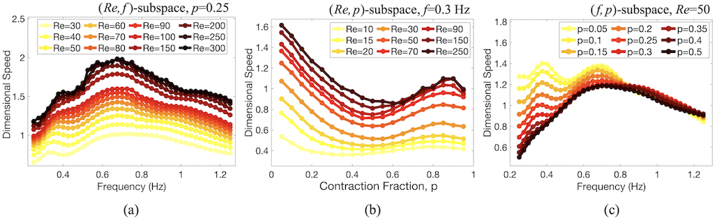
Figure 23: Dimensional forward swimming speed ($V_{dim}$) provided for different 2D parameter subspaces.

The dimensional cost of transport was also plotted against the dimensional forward swimming speed, see Figure 24. All of the simulation data corresponding to every 2D subspace study, i.e., Sections 3.2-3.4, is given in Figure 24a, whiles Figure 24b-d illustrate where different parameters lies across the performance space. Generally Figures 24c and 24d have distinct regions where certain data lies within the performance space for different frequencies and $\mathrm{Re}$, respectively. Lower $f$ generally resulted in lower cost of transport. Higher $\mathrm{Re}$ generally resulted in higher swimming speeds. However, both Figures 24b and 24c displayed that given a $p$ or $f$, combinations of the other two parameters, $(\mathrm{Re},f)$ or $(\mathrm{Re},p)$, respectively, could produce a jellyfish with any forward swimming speed in the performance space..

Figure 24: The dimensional average cost of transports and forward swimming speeds ($1/\mathrm{St}$) plotted against each other. (a) Data from all simulations, as well as highlighting regions within the performance landscape corresponding to different ranges of the input parameters: (b) different $\mathrm{Re}$ (c) different $f$, and (d) different $p$.

The dimensional data that complements Figure 13 is provided in Figure 25. The colormaps illustrate data for all 5000 sampled parameter combinations from the Sobol sensitivity analysis when projected onto the $(\mathrm{Re},f)$-subspaces (left column), $(\mathrm{Re},p$)-subspaces (middle column), or $(f,p)$-subspaces (right column), for both forward swimming speed and cost of transport. Patterns emerged within $(\mathrm{Re},f)$ and $(f,p)$ projected subspaces giving swimming speeds, where the trends aligned mostly with varying values of frequency, $f$. That is, variations in frequency led to the most significant overall changes in swimming speed. Variations in the cost of transport within the $(\mathrm{Re},f)$ projected subspace most aligned with changing frequency, as well. However, more nonlinear relationships emerged in the cost of transport within the $(f,p)$ projected subspace. Across the $(\mathrm{Re},p)$ projected subspace no discernible patterns emerged in either swimming speed or cost of transport.

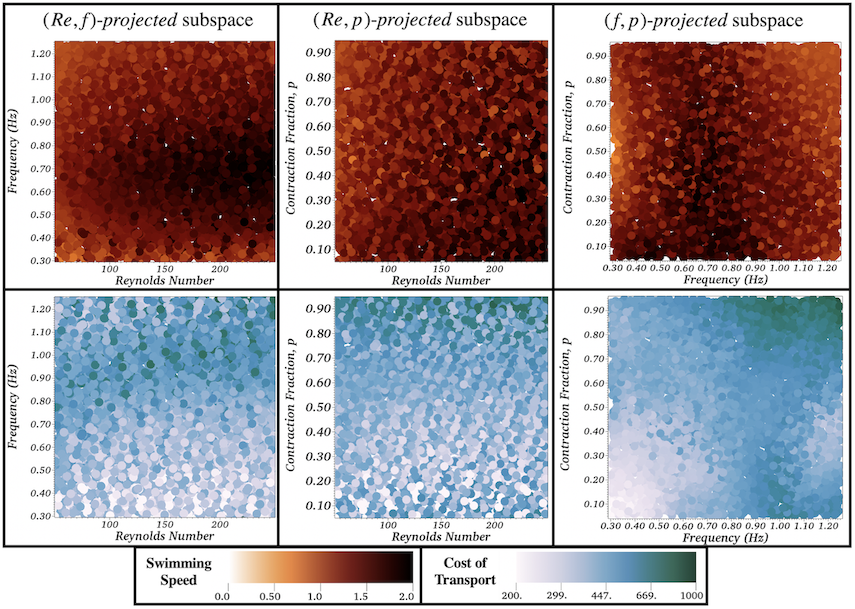
Figure 25: Colormaps of the projected data across all 5000 sampled parameter cases from the Sobol sequence giving the dimensional forward swimming speeds and cost of transports onto either the $(\mathrm{Re},f)$, $(\mathrm{Re},p)$, or $(f,p)$ subspace.

References

- (1) Akanyeti, O., Putney, J., Yanagitsuru, Y.R., Lauder, G.V., Stewart, W.J., Liao, J.C.: Accelerating fishes increase propulsive efficiency by modulating vortex ring geometry. PNAS 114(52), 13828–13833 (2017)
- (2) Alben, S., Miller, L.A., Peng, J.: Efficient kinematics for jet-propelled swimming. J. Fluid Mech. 733, 100–133 (2013)
- (3) Arai, M.N.: A Functional Biology of Scyphozoa. Springer Science & Business Media, Berlin/Heidelberg, Germany (1997)
- (4) Bainbridge, R.: The speed of swimming of fish as related to size and to the frequency and amplitude of the tail beat. Journal of Experimental Biology 35(1), 109–133 (1958). URL https://jeb.biologists.org/content/35/1/109
- (5) Bale, R., Hao, M., Bhalla, A., Patankar, N.A.: Energy efficiency and allometry of movement of swimming and flying animals. Proc. Natl. Acad. Sci. 111(21), 7517?7521 (2014)
- (6) Battista, N.A.: Diving into a simple anguilliform swimmer’s sensitivity. Int. Comp. Biol. p. icaa131 (2020). Accepted, in production
- (7) Battista, N.A.: Fluid-structure interaction for the classroom: Interpolation, hearts, and swimming! (accepted, in production) SIAM Review (2020)
- (8) Battista, N.A.: Swimming through parameter subspaces of a simple anguilliform swimmer. Int. Comp. Biol. p. icaa130 (2020). Accepted, in production
- (9) Battista, N.A., Baird, A.J., Miller, L.A.: A mathematical model and matlab code for muscle-fluid-structure simulations. Integr. Comp. Biol. 55(5), 901–911 (2015)
- (10) Battista, N.A., Lane, A.N., Liu, J., Miller, L.A.: Fluid dynamics of heart development: Effects of trabeculae and hematocrit. Math. Med. & Biol. 35, 493?516 (2017)
- (11) Battista, N.A., Mizuhara, M.S.: Fluid-structure interaction for the classroom: Speed, accuracy, convergence, and jellyfish! arXiv: https://arxiv.org/abs/1902.07615 (2019)
- (12) Battista, N.A., Strickland, W.C., Barrett, A., Miller, L.A.: IB2d Reloaded: a more powerful Python and MATLAB implementation of the immersed boundary method. Math. Method. Appl. Sci 41, 8455–8480 (2018)
- (13) Battista, N.A., Strickland, W.C., Miller, L.A.: IB2d: a Python and MATLAB implementation of the immersed boundary method. Bioinspir. Biomim. 12(3), 036003 (2017)
- (14) Berger, M.J., Oliger, J.: Adaptive mesh refinement for hyperbolic partial-differential equations. J. Comput. Phys. 53(3), 484–512 (1984)
- (15) Bhalla, A., Griffith, B.E., Patankar, N.: A forced damped oscillation framework for undulatory swimming provides new insights into how propulsion arises in active and passive swimming. PLOS Comput. Biol. 9, e1003097 (2013)
- (16) Bhalla, A., Griffith, B.E., Patankar, N.: A unified mathematical frame- work and an adaptive numerical method for fluid-structure interaction with rigid, deforming, and elastic bodies. J. Comput. Phys. 250, 446–476 (2013)
- (17) Blough, T., Colin, S.P., Costello, J.H., Marques, A.C.: Ontogenetic changes in the bell morphology and kinematics and swimming behavior of rowing medusae: the special case of the limnomedusa liriope tetraphylla. Biological Bulletin 220(1), 6–14 (2011). URL http://www.jstor.org/stable/20839320
- (18) Childs, H., Brugger, E., Whitlock, B., Meredith, J., Ahern, S., Pugmire, D., Biagas, K., Miller, M., Harrison, C., Weber, G.H., Krishnan, H., Fogal, T., Sanderson, A., Garth, C., Bethel, E.W., Camp, D., Rübel, O., Durant, M., Favre, J.M., Navrátil, P.: VisIt: An End-User Tool For Visualizing and Analyzing Very Large Data. In: E.W. Bethel, H. Childs, C. Hansen (eds.) High Performance Visualization–Enabling Extreme-Scale Scientific Insight, pp. 357–372. Chapman and Hall/CRC (2012)
- (19) Christianson, C., Bayag, C., Li, G., Jadhav, S., Giri, A., Agba, C., Li, T., Tolley, M.T.: Jellyfish-inspired soft robot driven by fluid electrode dielectric organic robotic actuators. Frontiers in Robotics and AI 6, 126 (2019). DOI 10.3389/frobt.2019.00126. URL https://www.frontiersin.org/article/10.3389/frobt.2019.00126
- (20) Colin, S.P., Costello, J.H.: Morphology, swimming performance and propulsive mode of six co-occurring hydromedusae. Journal of Experimental Biology 205(3), 427–437 (2002). URL https://jeb.biologists.org/content/205/3/427
- (21) Colin, S.P., Costello, J.H., Katija, K., Seymour, J., Kiefer, K.: Propulsion in cubomedusae: Mechanisms and utility. PLOS ONE 8(2), 1–12 (2013). DOI 10.1371/journal.pone.0056393. URL https://doi.org/10.1371/journal.pone.0056393
- (22) Cortez, R., Minion, M.: The blob projection method for immersed boundary problems. J. Comp. Phys. 161, 428–453 (2000)
- (23) Costello, J.H., Colin, S.P., Dabiri, J.O.: Medusan morphospace: Phylogenetic constraints, biomechanical solutions, and ecological consequences. Invertebrate Biology 127(3), 265–290 (2008). URL http://www.jstor.org/stable/40206199
- (24) Costello, J.H., Colin, S.P., Dabiri, J.O., Gemmell, B.J., Lucas, K.N., Sutherland, K.R.: The hydrodynamics of jellyfish swimming. Annual Review of Marine Science 13(1), null (2021). DOI 10.1146/annurev-marine-031120-091442. URL https://doi.org/10.1146/annurev-marine-031120-091442. PMID: 32600216
- (25) Dabiri, J.O., Colin, S.P., Costello, J.H.: Fast-swimming hydromedusae exploit velar kinematics to form an optimal vortex wake. J. Exp. Biol. 209, 2025–2033 (2006)
- (26) Dabiri, J.O., Colin, S.P., Costello, J.H.: Morphological diversity of medusan lineages constrained by animal–fluid interactions. Journal of Experimental Biology 210(11), 1868–1873 (2007). DOI 10.1242/jeb.003772. URL https://jeb.biologists.org/content/210/11/1868
- (27) Dabiri, J.O., Colin, S.P., Costello, J.H., Gharib, M.: Flow patterns generated by oblate medusan jellyfish: field measurements and laboratory analyses. J. Exp. Biol. 208, 1257–1265 (2005)
- (28) Dabiri, J.O., Colin, S.P., Katija, K., Costello, J.H.: A wake-based correlate of swimming performance and foraging behavior in seven co-occurring jellyfish species. Journal of Experimental Biology 213(8), 1217–1225 (2010). DOI 10.1242/jeb.034660. URL https://jeb.biologists.org/content/213/8/1217
- (29) Dabiri, J.O., Colin, S.P., Katija, K., Costello, J.H.: A wake-based correlate of swimming performance and foraging behavior in seven co-occurring jellyfish species. Journal of Experimental Biology 213(8), 1217–1225 (2010). DOI 10.1242/jeb.034660. URL https://jeb.biologists.org/content/213/8/1217
- (30) Dabiri, J.O., Gharib, M.: Sensitivity analysis of kinematic approximations in dynamic medusan swimming models. Journal of Experimental Biology 206(20), 3675–3680 (2003). DOI 10.1242/jeb.00597. URL https://jeb.biologists.org/content/206/20/3675
- (31) Demont, M.E., Gosline, J.M.: Mechanics of jet propulsion in the hydromedusan jellyfish, Polyorchis Pexicillatus: Iii. a natural resonating bell; the presence and importance of a resonant phenomenon in the locomotor structure. Journal of Experimental Biology 134(1), 347–361 (1988). URL https://jeb.biologists.org/content/134/1/347
- (32) Dular, J., Bajcar, T., Sirok, B.: Numerical investigation of flow in the vicinity of a swimming jellyfish. Eng. Appl. Comp. Fluid Mech. 3(2), 258–270 (2009)
- (33) E. Griffith, B., Luo, X.: Hybrid finite difference/finite element immersed boundary method. International Journal for Numerical Methods in Biomedical Engineering 33(12), e2888 (2017). DOI 10.1002/cnm.2888. URL https://onlinelibrary.wiley.com/doi/abs/10.1002/cnm.2888
- (34) Eloy, C.: On the best design for undulatory swimming. Journal of Fluid Mechanics 717, 48?89 (2013). DOI 10.1017/jfm.2012.561
- (35) Fauci, L., Fogelson, A.: Truncated newton methods and the modeling of complex immersed elastic structures. Commun. Pure Appl. Math 46, 787–818 (1993)
- (36) Floryan, D., Buren, T.V., Smits, A.J.: Swimmers’ wake structures are not reliable indicators of swimming performance. Bioinspiration & Biomimetics 15(2), 024001 (2020). DOI 10.1088/1748-3190/ab6fb9
- (37) Floryan, D., Van Buren, T., Smits, A.J.: Efficient cruising for swimming and flying animals is dictated by fluid drag. Proceedings of the National Academy of Sciences 115(32), 8116–8118 (2018). DOI 10.1073/pnas.1805941115. URL https://www.pnas.org/content/115/32/8116
- (38) Ford, M., Costello, J.: Kinematic comparison of bell contraction by four species of hydromedusae. Scientia Marina 64(S1), 47–53 (2000). DOI 10.3989/scimar.2000.64s147. URL http://scientiamarina.revistas.csic.es/index.php/scientiamarina/article/view/791
- (39) Frame, J., Lopez, N., Curet, O., Engeberg, E.D.: Thrust force characterization of free-swimming soft robotic jellyfish. Bioinspir. Biomim. 13(6), 064001 (2018)
- (40) Gemmell, B., Costello, J., Colin, S.P.: Exploring vortex enhancement and manipulation mechanisms in jellyfish that contributes to energetically efficient propulsion. Communicative & Integrative Biology 7, e29014 (2014)
- (41) Gemmell, B., Costello, J., Colin, S.P., Dabiri, J.: Suction-based propulsion as a basis for efficient animal swimming. Nature Communications 6, 8790 (2015)
- (42) Gemmell, B., Costello, J., Colin, S.P., Stewart, C., Dabiri, J., Tafti, D., Priya, S.: Passive energy recapture in jellyfish contributes to propulsive advantage over other metazoans. PNAS 110, 17904–17909 (2013)
- (43) Gordon, M.S., Blickhan, R., Dabiri, J.O., Videler, J.J.: Animal Locomotion: Physical Principles and Adaptations (1st edition). CRC Press, Boca Raton, FL USA (2017)
- (44) Gray, J.: Animal Locomotion (World Naturalist). Weidenfeld and Nicolson, London, UK (1968)
- (45) Griffith, B.E.: Immersed boundary model of aortic heart valve dynamics with physiological driving and loading conditions. Int. J. Numer. Meth. Biomed. Eng. 28(3), 317–345 (2012)
- (46) Griffith, B.E.: An adaptive and distributed-memory parallel implementation of the immersed boundary (ib) method (2014). URL https://github.com/IBAMR/IBAMR. [Online; accessed October 21, 2014]
- (47) Griffith, B.E., Hornung, R., McQueen, D., Peskin, C.S.: An adaptive, formally second order accurate version of the immersed boundary method. J. Comput. Phys. 223, 10–49 (2007)
- (48) Griffith, B.E., Peskin, C.S.: On the order of accuracy of the immersed boundary method: higher order convergence rates for sufficiently smooth problems. J. Comput. Phys 208, 75–105 (2005)
- (49) Hamlet, C., Fauci, L.J., Tytell, E.D.: The effect of intrinsic muscular nonlinearities on the energetics of locomotion in a computational model of an anguilliform swimmer. J. Theor. Biol. 385, 119–129 (2015)
- (50) Hamlet, C., Miller, L.A.: Feeding currents of the upside-down jellyfish in the presence of background flow. Bull. Math. Bio. 74(11), 2547–2569 (2012)
- (51) Herschlag, G., Miller, L.A.: Reynolds number limits for jet propulsion: a numerical study of simplified jellyfish. J. Theor. Biol. 285, 84–95 (2011)
- (52) Hoover, A.P., Griffith, B.E., Miller, L.A.: Quantifying performance in the medusan mechanospace with an actively swimming three-dimensional jellyfish model. J. Fluid. Mech. 813, 1112–1155 (2017)
- (53) Hoover, A.P., Miller, L.A.: A numerical study of the benefits of driving jellyfish bells at their natural frequency. J. Theor. Biol. 374, 13–25 (2015)
- (54) Hoover, A.P., Porras, A.J., Miller, L.A.: Pump or coast: the role of resonance and passive energy recapture in medusan swimming performance. J. Fluid. Mech. 863, 1031–1061 (2019)
- (55) Jones, S.K., Laurenza, R., Hedrick, T.L., Griffith, B.E., Miller, L.A.: Lift- vs. drag-based for vertical force production in the smallest flying insects. J. Theor. Biol. 384, 105–120 (2015)
- (56) Joshi, K.B.: Modeling of bio-inspired jellyfish vehicle for energy efficient propulsion (Ph.D. Thesis). College of Engineering, Virginia Polytechnic Institute (2012)
- (57) Katija, K.: Morphology alters fluid transport and the ability of organisms to mix oceanic waters. Int. Comp. Biol. 55(4), 698–705 (2015)
- (58) Katija, K., Colin, S.P., Costello, J.H., Jiang, H.: Ontogenetic propulsive transitions by Sarsia tubulosa medusae. J. Exp. Biol 218, 2333–2343 (2015)
- (59) Katija, K., Jiang, H.: Swimming by medusae Sarsia tubulosa in the viscous vortex ring limit. Limnology and Oceanography: Fluids and Environments 3(1), 103–118 (2013). DOI 10.1215/21573689-2338313. URL https://aslopubs.onlinelibrary.wiley.com/doi/abs/10.1215/21573689-2338313
- (60) Kim, Y., Peskin, C.S.: 2d parachute simulation by the immersed boundary method. SIAM J. Sci. Comput. 28, 2294–2312 (2006)
- (61) Klotsa, D.: As above, so below, and also in between: mesoscale active matter in fluids. Soft Matter 15, 8946–8950 (2019)
- (62) Lai, M.C., Peskin, C.S.: An immersed boundary method with formal second-order accuracy and reduced numerical viscosity. J. Comp. Phys. 160, 705–719 (2000)
- (63) Link, K.G., Stobb, M.T., Di Paola, J., Neeves, K.B., Fogelson, A.L., Sindi, S.S., Leiderman, K.: A local and global sensitivity analysis of a mathematical model of coagulation and platelet deposition under flow. PLOS ONE 13(7), e0200917 (2018)
- (64) Lipinski, D., Mohseni, K.: Flow structures and fluid transport for the hydromedusae Sarsia tubulosa and Aequorea victoria. J. Exp. Biol. 212, 2436–2447 (2009)
- (65) MATLAB: version 8.5.0 (R2015a). The MathWorks Inc., Natick, Massachusetts, USA (2015)
- (66) McHenry, M.J.: Comparative biomechanics: The jellyfish paradox resolved. Current Biology 17(16), R632 – R633 (2007)
- (67) McHenry, M.J., Jed, J.: The ontogenetic scaling of hydrodynamics and swimming performance in jellyfish (Aurelia aurita). Journal of Experimental Biology 206(22), 4125–4137 (2003). DOI 10.1242/jeb.00649. URL https://jeb.biologists.org/content/206/22/4125
- (68) Miles, J.G., Battista, N.A.: Naut your everyday jellyfish model: Exploring how tentacles and oral arms impact locomotion. Fluids 4(3), 169 (2019)
- (69) Miller, L.A.: Fluid dynamics of ventricular filling in the embryonic heart. Cell Biochem. Biophys. 61, 33–45 (2011)
- (70) Miller, L.A., Peskin, C.S.: When vortices stick: an aerodynamic transition in tiny insect flight. J. Exp. Biol. 207, 3073–3088 (2004)
- (71) Miller, L.A., Peskin, C.S.: A computational fluid dynamics of clap and fling in the smallest insects. J. Exp. Biol. 208, 3076–3090 (2005)
- (72) Mittal, R., Iaccarino, C.: Immersed boundary methods. Annu. Rev. Fluid Mech. 37, 239–261 (2005)
- (73) Neil, T.R., Askew, G.N.: Jet-paddling jellies: swimming performance in the rhizostomeae jellyfish catostylus mosaicus. Journal of Experimental Biology 221(24) (2018). DOI 10.1242/jeb.191148. URL https://jeb.biologists.org/content/221/24/jeb191148
- (74) Nossent, J., Elsen, P., Bauwens, W.: Sobol? sensitivity analysis of a complex environmental model. Envir. Model. Soft. 26(12), 1515–1525 (2011)
- (75) Pallasdies, F., Goedeke, S., Braun, W., Memmesheimer, R.M.: From single neurons to behavior in the jellyfish Aurelia aurita. eLife 8, e50084 (2019). DOI 10.7554/eLife.50084. URL https://doi.org/10.7554/eLife.50084
- (76) Pang, K., Martindale, M.Q.: Ctenophores. Current Biology 18(24), R1120–R1119 (2008)
- (77) Park, S.G., Chang, C.B., Huang, W.X., Sung, H.J.: Simulation of swimming oblate jellyfish with a paddling-based locomotion. Journal of Fluid Mechanics 748, 731?755 (2014). DOI 10.1017/jfm.2014.206
- (78) Park, S.G., Kim, B., Lee, J., Huang, W.X., Sung, H.J.: Dynamics of prolate jellyfish with a jet-based locomotion. Journal of Fluids and Structures 57, 331 – 343 (2015). DOI https://doi.org/10.1016/j.jfluidstructs.2015.07.002. URL http://www.sciencedirect.com/science/article/pii/S0889974615001620
- (79) Peng, J., Alben, S.: Effects of shape and stroke parameters on the propulsion performance of an axisymmetric swimmer. Bioinspiration & Biomimetics 7(1), 016012 (2012). DOI 10.1088/1748-3182/7/1/016012
- (80) Peskin, C.: Flow patterns around heart valves: A numerical method. J. Comput. Phys. 10(2), 252–271 (1972)
- (81) Peskin, C.: Numerical analysis of blood flow in the heart. J. Comput. Phys. 25, 220–252 (1977)
- (82) Peskin, C.S.: The immersed boundary method. Acta Numerica 11, 479–517 (2002)
- (83) Ren, Z., Hu, W., Dong, X., Sitti, M.: Multi-functional soft-bodied jellyfish-like swimming. Nature Commun. 10, 2703 (2019). URL https://doi.org/10.1038/s41467-019-10549-7
- (84) Roma, A.M., Peskin, C.S., Berger, M.J.: An adaptive version of the immersed boundary method. J. Comp. Phys. 153, 509–534 (1999)
- (85) Rudolf, D., Mould, D.: An interactive fluid model of jellyfish for animation. In: A.K. Ranchordas, J.M. Pereira, H.J. Araújo, J.M.R.S. Tavares (eds.) Computer Vision, Imaging and Computer Graphics. Theory and Applications, pp. 59–72. Springer Berlin Heidelberg, Berlin, Heidelberg (2010)
- (86) Sahin, M., Mohseni, K.: An arbitrary lagrangian-eulerian formulation for the numerical simulation of flow patterns generated by the hydromedusa aequorea victoria. Journal of Computational Physics 228(12), 4588 – 4605 (2009). DOI https://doi.org/10.1016/j.jcp.2009.03.027. URL http://www.sciencedirect.com/science/article/pii/S0021999109001570
- (87) Sahin, M., Mohseni, K., Colin, S.P.: The numerical comparison of flow patterns and propulsive performances for the hydromedusae Sarsia tubulosa and Aequorea victoria. Journal of Experimental Biology 212(16), 2656–2667 (2009). DOI 10.1242/jeb.025536. URL https://jeb.biologists.org/content/212/16/2656
- (88) Saltelli, A.: Making best use of model evaluations to compute sensitivity indices. Comp. Phys. Comm. 145(2), 280–297 (2002)
- (89) Saltelli, A., Aleksankina, K., Becker, W., Fennell, P., Ferretti, F., Holst, N., Li, S., Wu, Q.: Why so many published sensitivity analyses are false: A systematic review of sensitivity analysis practices. Environ. Model. & Software 114, 29 – 39 (2019)
- (90) Saltelli, A., Annoni, P., Azzini, I., Campolongo, F., Ratto, M., Tarantola, S.: Variance based sensitivity analysis of model output. design and estimator for the total sensitivity index. Comp. Phys. Comm. 18(2), 259–270 (2010)
- (91) Santhanakrishnan, A., Dollinger, M., Hamlet, C.L., Colin, S.P., Miller, L.A.: Flow structure and transport characteristics of feeding and exchange currents generated by upside-down cassiopea jellyfish. J. Exp. Biol. 215, 2369–2381 (2011)
- (92) Satterlie, R.A.: Do jellyfish have central nervous systems? J. Exp. Biol. 214, 1215–1223 (2011)
- (93) Schmidt-Nielsen, K.: Locomotion: energy cost of swimming, flying, and running. Science 177, 222–228 (1972)
- (94) Schuech, R., Hoehfurtner, T., Smith, D.J., Humphries, S.: Motile curved bacteria are pareto-optimal. PNAS 116(29), 14440–14447 (2019)
- (95) Smits, A.J.: Undulatory and oscillatory swimming. Journal of Fluid Mechanics 874, P1 (2019). DOI 10.1017/jfm.2019.284
- (96) Sobol, I.M.: Global sensitivity indices for nonlinear mathematical models and their Monte Carlo estimates. Math. and Comput. in Simul. 55(1-3), 271–280 (2001)
- (97) Steinhausen, M.F., Steffensen, J.F., Andersen, N.G.: Tail beat frequency as a predictor of swimming speed and oxygen consumption of saithe (Pollachius virens) and whiting (Merlangius merlangus) during forced swimming. Marine Biology 148, 197–204 (2005)
- (98) Sudret, B.: Global sensitivity analysis using polynomial chaos expansions. Reliability Engineering & System Safety 93(7), 964–979 (2008)
- (99) Taylor, G.K., Nudds, R.L., Thomas, A.L.: Flying and swimming animals cruise at a Strouhal number tuned for high power efficiency. Nature 425, 707–711 (2003)
- (100) The College of New Jersey: Electronic laboratory for science & analysis (elsa) (2020). URL https://docs.hpc.tcnj.edu/. Accessed Online; accessed 24 January 2020
- (101) Triantafyllou, M.S., Triantafyllou, G.S., Gopalkrishnan, R.: Wake mechanics for thrust generation in oscillating foils. Physics of Fluids A: Fluid Dynamics 3(12), 2835–2837 (1991). DOI 10.1063/1.858173. URL https://doi.org/10.1063/1.858173
- (102) Verma, S., Hadjidoukas, P., Wirth, P., Rossinelli, D., Koumoutsakos, P.: Pareto optimal swimmers. In: Proceedings of the Platform for Advanced Scientific Computing Conference, PASC ?17. Association for Computing Machinery, New York, NY, USA (2017). URL https://doi.org/10.1145/3093172.3093232
- (103) Videler, J.J., Weihs, D.: Energetic advantages of burst-and-coast swimming of fish at high speeds. Journal of Experimental Biology 97(1), 169–178 (1982). URL https://jeb.biologists.org/content/97/1/169
- (104) Vogel, S.: Life in Moving Fluids: The Physical Biology of Flow. Princeton Paperbacks, Princeton, NJ, USA (1996)
- (105) Waldrop, L.D., He, Y., Battista, N.A., Neary, T., Miller, L.A.: Uncertainty quantification reveals the physical constraints on pumping by valveless, tubular hearts. J. Royal Society Interface 17, 20200232 (2020)
- (106) Waldrop, L.D., He, Y., Hedrick, T.L., Rader, J.: Functional morphology of gliding flight I. Modeling reveals distinct performance landscapes based on soaring strategies. Integrative and Comparative Biology (2020)
- (107) Waldrop, L.D., He, Y., Khatri, S.: What can computational modeling tell us about the diversity of odor-capture structures in the pancrustacea? J. Chem. Ecol. 44, 1084–1100 (2018)
- (108) Weston, J., Colin, S.P., Costello, J.H., Abbott, E.: Changing form and function during development in rowing hydromedusae. Mar Ecol Prog Ser 374, 127–134 (2009)
- (109) Wilson, M.M., Eldredge, J.D.: Performance improvement through passive mechanics in jellyfish-inspired swimming. International Journal of Non-Linear Mechanics 46(4), 557 – 567 (2011). DOI https://doi.org/10.1016/j.ijnonlinmec.2010.12.005. Special issue on non-linear mechanics of biological structures
- (110) Wilson, M.M., Peng, J., Dabiri, J.O., Eldredge, J.D.: Lagrangian coherent structures in low Reynolds number swimming. Journal of Physics: Condensed Matter 21(20), 204105 (2009). DOI 10.1088/0953-8984/21/20/204105
- (111) Xiu, D., Karniadakis, G.E.: Modeling uncertainty in flow simulations via generalized polynomial chaos. J. Comp. Phys. 187, 137–167 (2003)
- (112) Xiu, D., Lucor, D., Su, C.H., Karniadakis, G.E.: Performance evaluation of generalized polynomial chaos. In: P. Sloot, D. Abramson, A.V. Bogdanov, Y.E. Gorbachev, J.J. Dongarra, A.Y.Z. A.Y. (eds.) In International Conference on Computational Science, chap. 36, pp. 346–354. Springer, Berlin, Heidelberg, Germany (2003)
- (113) Xu, N.W., Dabiri, J.O.: Low-power microelectronics embedded in live jellyfish enhance propulsion. Science Advances 6(5) (2020). DOI 10.1126/sciadv.aaz3194. URL https://advances.sciencemag.org/content/6/5/eaaz3194
- (114) Yuan, H., Shu, S., Niu, X., Li, M.: A Numerical Study of Jet Propulsion of an Oblate Jellyfish Using a Momentum Exchange-Based Immersed Boundary-Lattice Boltzmann Method. Adv. in Appl. Math. and Mech. 6(3), 307–326 (2014)