Deep Convolutional Neural Network and Sparse Least Squares Migration

Abstract

We recast the forward pass of a multilayered convolutional neural network (CNN) as the solution to the problem of sparse least squares migration (LSM). The CNN filters and feature maps are shown to be analogous, but not equivalent, to the migration Green’s functions and the quasi-reflectivity distribution, respectively. This provides a physical interpretation of the filters and feature maps in deep CNN in terms of the operators for seismic imaging. Motivated by the connection between sparse LSM and CNN, we propose the neural network version of sparse LSM. Unlike the standard LSM method that finds the optimal reflectivity image, neural network LSM (NNLSM) finds both the optimal quasi-reflectivity image and the quasi-migration Green’s functions. These quasi-migration-Green’s functions are also denoted as the convolutional filters in a CNN and are similar to migration Green’s functions. The advantage of NNLSM over standard LSM is that its computational cost is significantly less and it can be used for denoising coherent and incoherent noise in migration images. Its disadvantage is that the NNLSM quasi-reflectivity image is only an approximation to the actual reflectivity distribution. However, the quasi-reflectivity image can be used as a superresolution attribute image for high-resolution delineation of geologic bodies.

1 Introduction

Deep convolutional neural networks (CNNs) have been recently used for solving geophysical problems, such as seismic first-arrival picking (Lu and Feng,, 2018; Yuan et al.,, 2018; Hu et al.,, 2019), seismic interpretation (Wu et al., 2019a, ; Wu et al., 2019b, ; Shi et al.,, 2019), and seismic imaging and inversion (Xu et al.,, 2019; Sun et al.,, 2020; Kaur et al.,, 2020). Interpretation examples include salt classification (Waldeland et al.,, 2018; Shi et al.,, 2019), fault detection (Huang et al.,, 2017; Xiong et al.,, 2018; Wu et al., 2019b, ; Zheng et al.,, 2019), reservoir characterization (Karimpouli et al.,, 2010; Cao and Roy,, 2017; Zhu et al.,, 2017), and seismic lithofacies classification (Ross and Cole,, 2017; Liu et al.,, 2019) with semi-supervised learning (Di et al.,, 2020). Other applications include the use of neural networks for well-log interpolation (Saggaf and Nebrija,, 2003; Salehi et al.,, 2017; Pham et al.,, 2020), seismic data interpolation (Mandelli et al.,, 2018, 2019; Wang et al.,, 2020), velocity model building (Araya-Polo et al.,, 2018; Richardson,, 2018), well-log ties (Bader et al.,, 2019), synthetic well-data generation (Rolon et al.,, 2009), autoencoders for unsupervised facies analysis (Qian et al.,, 2018), and supervised horizon tracking (Peters et al., 2019a, ; Peters et al., 2019b, ). Recently, an unsupervised autoencoder method with regularization was developed by Shi et al., (2020) to track target horizons.

There are many types of neural network or machine learning methods, selections ranging from generative adversarial networks for seismic interpolation (Siahkoohi et al.,, 2018), residual networks for traces missing at regular intervals (Wang et al.,, 2019), Monte Carlo and support vector regression (Jia et al.,, 2018) for data interpolation, autoencoders (Wang et al.,, 2020; Shi et al.,, 2020) for target horizons tracking, and recurrent neural networks for well-log interpolation (Pham et al.,, 2020). The design of geophysical CNN architectures has largely been based on empirical evidence from computer vision research, insights from the principles of artificial intelligence and heuristic experimentation. Heuristic experimentation is most often used to decide the parameter design for the CNN architecture, which has both merits and liabilities. The merit is that trial-and-error with different architecture parameters is likely to give excellent results for a particular data set, but it might not be the best one for a completely different data set. This shortcoming in using empirical tests for parameter selection largely results from the absence of a rigorous mathematical foundation (Papyan et al.,, 2016; Papyan et al., 2017a, ) for neural networks in general, and CNN in particular.

To mitigate this problem for CNN-based imaging algorithms, we now present a physical interpretation of the CNN filters and feature maps in terms of the physics-based operators for seismic imaging. With such an understanding, we can use a physics-based rationale for the better design of CNN architectures in seismic migration and inversion.

Donoho, (2019) points out that “machine learning has a troubled relationship with understanding the foundation of its achievements well and its literature is admittedly corrupted by anti-intellectual and anti-scholarly tendencies”. Progress in advancing the capabilities of deep neural networks will be severely stymied unless its mathematical foundations are established. As a first step in this direction, Papyan et al., (2016) proposed that the forward modeling operation of CNN could be recast as finding the sparsest model ${\bf m}$ under the $L_{1}$ norm subject to honoring the data misfit constraint $||{{\bm{\Gamma}}{\bf m}-{\bf d}}||_{2}^{2}\leq\beta$:

$$Given: {\bm{\Gamma}},{\bf d}~{}~{}~{}~{}\mbox{and}~{}~{}{{\bm{\Gamma}}{\bf m}}={{\bf d}}+\bm{noise},$$

$$Find: {{\bf m}^{*}}=\arg\min_{{\bf m}}||{\bf m}||_{1}~{}~{}~{}~{}$$ (1)

$$\mbox{subject~{}to}~{}||{{\bm{\Gamma}}{\bf m}-{\bf d}}||_{2}^{2}\leq\beta\,$$

where ${\bf m}^{*}$ is the optimal solution of ${\bf m}$, ${\bm{\Gamma}}$ is the dictionary matrix, ${\bf d}$ represents the signal, and the scalar $\beta$ is the specified noise tolerance. The iterative solution to this problem is a series of forward-modeling operations of a neural network, where the mathematical operations of each layer consist two steps: a weighted summation of input values to give the vector ${\bf z}$ followed by a two-sided soft thresholding operation denoted as $\sigma({{\bf z}})$ (Papyan et al.,, 2016).

The sparse constraint problem defined in equation 1 is commonly seen in geophysics, for example, the least square migration (LSM) with a sparse constraint. LSM is an important seismic-imaging technique to produce images with better balanced amplitudes, fewer artifacts and better resolution than standard migration (Lailly,, 1983; Tarantola,, 1987; Schuster,, 1993; Nemeth et al.,, 1999; Chavent and Plessix,, 1999; Duquet et al.,, 2000; Feng and Schuster,, 2017; Schuster and Liu,, 2019). The sparse constraint is one of the important regularization terms used in solving the ill-conditioned least-squares problem (Sacchi and Ulrych,, 1995; De Roeck,, 2002; Kühl and Sacchi,, 2003; Wang and Sacchi,, 2005) and sparse LSM (SLSM) has been demonstrated to be effective for mitigation of aliasing artifacts and crosstalk in LSM (Wang and Sacchi,, 2007; Herrmann et al.,, 2009; Dutta,, 2017; Witte et al.,, 2017; Li and Gao,, 2018). The image-domain SLSM finds the sparsest reflectivity ${\bf m}^{*}$ with sparse constraints to minimize the objective function $||{{\bm{\Gamma}}{\bf m}-{\bf m}^{mig}}||_{2}^{2}$, where $\bm{\Gamma}$ is the Hessian matrix and ${\bf m}^{mig}$ is the migration image. Here, we can see SLSM shares the same problem as that defined in equation  1. Following the work of Papyan et al., (2016), we show that the sparse solution to the LSM problem reduces to the forward modeling operations of a multilayered neural network. The CNN filters and feature maps are shown to be analogous, but not equivalent, to the migration Green’s functions (Hessian) and the reflectivity distribution.

The standard SLSM algorithm needs to solve the wave equation, which is time-consuming. Motivated by the connection between sparse LSM and CNN, we propose the neural network version of sparse LSM, which does not need to solve the wave equation and is faster than standard SLSM. Instead of just finding the optimal reflectivity ${\bf m}^{*}$, we optimize for both the quasi-reflectivity $\bf m$ and the quasi-migration-Green’s functions $\bm{\Gamma}$. These quasi-migration-Green’s functions approximate the role of migration Green’s function (Schuster and Hu,, 2000) and are denoted as the convolutional filters in a convolutional neural network. As discussed in Appendix LABEL:A, the migration Green’s function is the point-scatterer response of the migration operator. The final image is denoted as the neural network least squares migration (NNLSM) estimate of the quasi-reflectivity distribution that honors the $L_{1}$ sparsity condition. The next section shows the connection between the multilayer neural network and the solution to the multilayer NNLSM problem. This is followed by the numerical examples with the synthetic models and field data from the North Sea.

2 Theory of Neural Network Least Squares Migration

The theory of standard image-domain LSM is first presented to establish the benchmark solution where the optimal reflectivity function minimizes the image misfit under the $L_{2}$ norm. This is then followed by the derivation of the sparse least squares migration (SLSM) solution for a single-layer network. The final two subsections derive the NNLSM solution for single-layer and multilayer networks, respectively.

2.1 Least Squares Migration

The least squares migration (LSM) problem can be defined (Schuster and Hu,, 2000; Schuster,, 2017) as finding the reflectivity coefficients $m_{i}$ in the $N\times 1$ vector ${\bf m}$ that minimize the $L_{2}$ objective function $\epsilon=1/2||{\bm{\Gamma}}{\bf m}-{\bf m}^{mig}||_{2}^{2}$,

$${\bf m}^{*} = \arg\min_{{\bf m}}\{\frac{1}{2}||{\bm{\Gamma}}{\bf m}-{\bf m}^{mig}||_{2}^{2}\},$$ (2)

where ${\bm{\Gamma}}={\bf L}^{T}{\bf L}$ is the symmetric $N\times N$ Hessian matrix, ${\bf L}$ is the forward modeling operator, and ${\bf L}^{T}$ is the migration operator. Here, ${\bf m}^{mig}={{\bf L}^{T}}{\bf d}$ is the migration image computed by migrating the recorded data ${\bf d}$ with the migration operator ${\bf L}^{T}$. Alternatively, the image-domain LSM problem can also be defined as finding $\bf m$ that minimizes $\epsilon=1/2({\bf m}^{T}{\bm{\Gamma}}{\bf m}-{\bf m}^{T}{\bf m}^{mig})$, which has a more well-conditioned solution than the one in equation 2 (Schuster,, 2017). However, we will use equation 2 as the definition of the LSM problem in order to be consistent with the notation from Papyan et al., 2017a . The kernel associated with the Hessian matrix ${\bf L}^{T}{\bf L}$ is also known as the point scatterer response of the migration operator or the migration Green’s function (Schuster and Hu,, 2000). It is a square matrix that is assumed to be invertible, otherwise a regularization term is incorporated into the objective function.

A formal solution to equation 2 is

$${\bf m}^{*} = {\bm{\Gamma}}^{-1}{\bf m}^{mig},$$ (3)

where it is too expensive to directly compute the inverse Hessian ${\bm{\Gamma}}^{-1}$. Instead, a gradient method gives the iterative solution

$${\bf m}^{(k+1)} = {\bf m}^{(k)}-\alpha{\bm{\Gamma}}^{T}({\bm{\Gamma}}{\bf m}^{(k)}-{\bf m}^{mig}),$$ (4)

where $\alpha$ is the step length, $\bm{\Gamma}$ is symmetric, and ${\bf m}^{(k)}$ is the solution at the $k^{th}$ iteration. Typically, a regularization term is used to stabilize the solution, for example, the sparse constraint which will be introduced in the next subsection.

2.2 Sparse Least Squares Migration

The sparse least squares migration (SLSM) in the image domain is defined as finding the reflectivity coefficients $m_{i}$ in the $N\times 1$ vector ${\bf m}$ that minimize the objective function $\epsilon$ (Perez et al.,, 2013):

$$\epsilon = \frac{1}{2}||{\bm{\Gamma}}{\bf m}-{\bf m}^{mig}||_{2}^{2}+\lambda S({\bf m}),$$ (5)

where ${\bm{\Gamma}}={\bf L}^{T}{\bf L}$ represents the migration Green’s function (Schuster and Hu,, 2000), $\lambda>0$ is a positive scalar, ${\bf m}^{mig}={{\bf L}^{T}}{\bf d}$ is the migration image, and $S({\bf m})$ is a sparseness function. For example, the sparseness function might be $S({\bf m})=||{\bf m}||_{1}$ or $S({\bf m})=log(1+||{\bf m}||_{2}^{2})$.

The solution to equation 5 is

$${\bf m}^{*} = \arg\min_{{\bf m}}{\Big{[}}\frac{1}{2}||{\bm{\Gamma}}{\bf m}-{\bf m}^{mig}||_{2}^{2}+\lambda S({\bf m}){\Big{]}},$$ (6)

which can be approximated by an iterative gradient descent method:

$$m_{i}^{(k+1)} = m_{i}^{(k)}-\alpha{\Big{[}}{\bm{\Gamma}}^{T}\overbrace{({\bm{\Gamma}}{\bf m}-{\bf m}^{mig})}^{{\bf r}=residual}+\lambda S({\bf m})^{\prime}{\Big{]}}_{i},$$ (7)

$$= m_{i}^{(k)}-\alpha[{\bm{\Gamma}}^{T}{\bf r}+\lambda S({\bf m})^{\prime}]_{i}.$$

Here, $S({\bf m})_{i}^{\prime}$ is the derivative of the sparseness function with respect to the model parameter $m_{i}$ and the step length is $\alpha$. Vectors and matrices are denoted by boldface lowercase and uppercase letters, respectively. When $S({\bf m})=||{\bf m}||_{1}$, the iterative solution in equation 7 can be recast as

$$m_{i}^{(k+1)}={\mbox{soft}}({\Big{[}}{\bf m}^{(k)}-\frac{1}{\alpha}{\bm{\Gamma}}^{T}({\bm{\Gamma}}{\bf m}^{(k)}-{\bf m}_{mig}){\Big{]}}_{i},\frac{\lambda}{\alpha}),$$ (8)

where, soft is the two-sided soft thresholding function (Papyan et al.,, 2016) derived in Appendix LABEL:B (see equation 22). Here, $\bm{\Gamma}={\bf L}^{T}{\bf L}$ is computed by solving the wave equation to get the forward modeled field and backpropagating the data by a numerical solution to the adjoint wave equation.

Equation 8 is similar to the forward modeling operation associated with the first layer of the neural network in Figure 1. That is, set $k=0$, ${\bf m}^{(0)}=0$, $\alpha=1$, and let the input vector be the scaled residual vector ${\bf r}=-({\bm{\Gamma}}{\bf m}^{(0)}-{\bf m}_{mig})={\bf m}_{mig}$ so that the first-iterate solution can be compactly represented by

$${\bf m}^{(1)}=\mbox{soft}({\bm{\Gamma}}^{T}{\bf m}^{mig},\lambda).$$ (9)

Here, the input vector ${\bf r}={\bf m}^{mig}$ is multiplied by the matrix ${\bm{\Gamma}}^{T}$ to give ${\bf z}={\bm{\Gamma}}^{T}{\bf r}$, and the elements of = ${\bf z}$ are then thresholded and shrunk to give the output ${{\bf m}}=\mbox{soft}({\bf z},\lambda)$. If we impose a positivity constraint for ${\bf z}$ and a shrinkage constraint so $\lambda$ is small, then the soft thresholding function becomes that of a one-sided threshold function, also known as the Rectified Linear Unit or ReLU function. To simplify the notation, the $\mbox{soft}({\bf z},\lambda)$ function or $\mbox{ReLu}({\bf z})$ function is replaced by $\sigma_{\lambda}({\bf z})$ so that equation 9 is given by

$${\bf m}^{(1)}=\sigma_{\lambda}({\bm{\Gamma}}^{T}{\bf m}^{mig}).$$ (10)

For the ReLu function there is no shrinkage so $\lambda=0$. However, $\bm{\Gamma}$ in equation 10 is computed by forward and backward solutions to the wave equation. Unlike a neural network, the physics of wave propagation is included with the sparse LSM solution in equation 8.

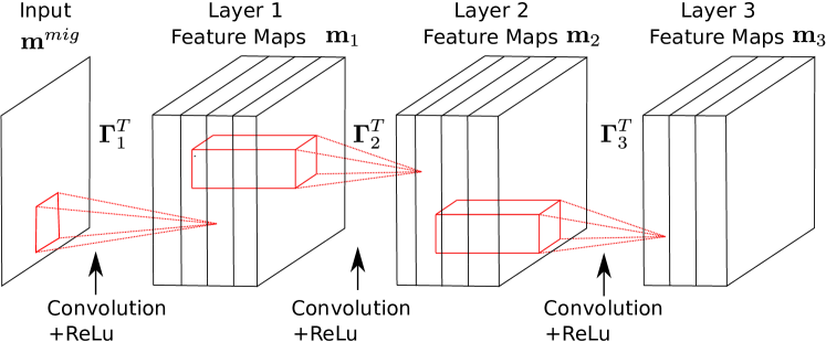
Figure 1: The forward modeling procedure for a multilayer CNN is equivalent to the multilayer sparse solution.

2.3 Neural Network Least Squares Migration

We now propose the neural network version of SLSM that finds both $\bm{\Gamma}^{*}$ and ${\bf m}^{*}$ which minimize equation 5, which is equivalent to the convolutional sparse coding (CSC) problem. We denote the optimal solution $\bf m$ as the neural network least squares migration (NNLSM) image. Here, we assume that the migration image ${\bf m}^{mig}$ can be decomposed into components that have the form ${\bm{\Gamma}}_{1}{\bf m}_{1}$, where ${\bf m}_{1}$ represents a sparse quasi-reflectivity structure for the $1^{th}$ CNN layer in Figure 1 and ${\bm{\Gamma}}_{1}$ has a convolutional structure. The solution can be found by using the Alternating Direction Method of Multipliers (ADMM) method either in the Fourier domain (Heide et al.,, 2015) or in the space domain (Papyan et al., 2017b, ), which alternates between finding $\bm{\Gamma}^{*}$ (dictionary learning problem) and then finding ${\bf m}^{*}$ (sparse pursuit problem). The key difference between least squares sparse inversion and NNLSM is that $\bm{\Gamma}$ is not computed by numerical solutions to the wave equation. Instead, the coefficients of $\bm{\Gamma}$ are computed by the usual gradient-descent learning algorithm of a convolutional neural network. For this reason, we denote $\bf m^{*}$ as the quasi-reflectivity distribution and $\bm{\Gamma}^{*}$ as the quasi-migration Green’s function.

Appendix LABEL:C shows the general solution for NNLSM for a single-layer neural network, where the optimal $\bm{\Gamma}^{*}$ is composed of the quasi-migration Green’s functions, which are denoted as convolutional filters in the machine learning terminology (Liu and Schuster,, 2018, 2019). Each filter is used to compute a feature map that corresponds to a sub-image of quasi-reflection coefficients in the context of LSM.

We now compute the NNLSM image for a 1D model, where we assume ${\bf m}^{mig}$ is a N-dimensional vector which can be expressed as,

$${\bf m}^{mig}=\sum_{i}^{k_{0}}{\bm{\gamma}}_{i}*{\bf m}_{1i}^{\prime}.$$ (11)

Here, ${\bm{\gamma}}_{i}$ is the $i^{th}$ local filter with length of $n_{0}$, ${\bf m}^{\prime}_{1i}$ is the $i^{th}$ feature map, “*” denotes the convolution operator and $k_{0}$ is the number of the filters. Alternatively, following Figure 2a, equation 11 can be written in matrix form as ${\bf m}^{mig}={\bm{\Gamma}}_{1}{\bf m}_{1}={\bm{\Gamma}}_{1}^{\prime}{\bf m}_{1}^{\prime}$ (Papyan et al., 2017a, ), where ${\bm{\Gamma}}_{1}$ is a convolutional matrix containing in its columns the $k_{0}$ filters with all of their shifts. ${\bm{\Gamma}}_{1}^{\prime}$ is a concatenation of banded and circulant matrices, which is the same as ${\bm{\Gamma}}_{1}$ except that the order of the columns is different. ${\bf m}_{1}^{\prime}$ is a concatenation of the feature map vectors ${\bf m}_{1i}^{\prime}$ for $i=1,2,\cdots,k_{0}$.

The advantage of NNLSM is that only inexpensive matrix-vector multiplications are used and no expensive solutions to the wave equation are needed for backward and forward wavefield propagation. As will be seen later, convolutional filters that appear to be coherent noise can be excluded for denoising the migration image.

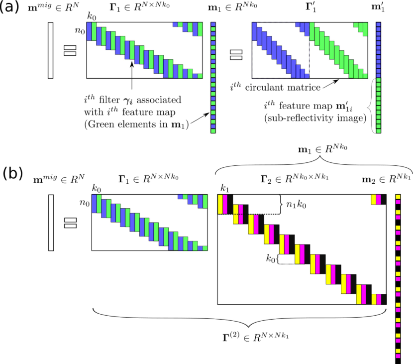
Figure 2: (a) Single-layer NNLSM and (b) multilayer NNLSM for a one-dimensional migration image ${\bf m}^{mig}$.

2.4 Multilayer Neural Network LSM

The multilayer NNLSM is a natural extension of the single-layer NNLSM. For NNLSM, the migration image ${\bf m}^{mig}$ can be expressed as ${\bf m}^{mig}={\bm{\Gamma}}_{1}{\bf m}_{1}$ (Figure 2a), where there are $k_{0}$ filters in ${\bm{\Gamma}}_{1}$ and $k_{0}$ sub-quasi-reflectivity images in ${\bf m}_{1}$. Following Sulam et al., (2018), we can cascade this model by imposing a similar assumption to the sparse representation ${\bf m}_{1}$, i.e., ${\bf m}_{1}={\bm{\Gamma}}_{2}{\bf m}_{2}$, for a corresponding convolutional matrix ${\bm{\Gamma}}_{2}$ with $k_{1}$ local filters and a sparse sub-quasi-reflectivity image ${\bf m}_{2}$, as depicted in Figure 2b. In this case, the filter size is $n_{1}\times k_{0}$ and there are $k_{1}$ sub-quasi-reflectivity images in ${\bf m}_{2}$.

Similar to the derivation by Papyan et al., 2017a and Sulam et al., (2018), the multilayer neural network LSM problem is defined as the following.

Find: $${\bf m}_{i},\Gamma_{i}~{}~{}~{}\mbox{such~{}that}$$

$${\bf m}_{1}^{*} = \arg\min_{{\bf m}_{1},\Gamma_{1}}{\Big{[}}\frac{1}{2}||{\bm{\Gamma}}_{1}{\bf m}_{1}-{\bf m}^{mig}||_{2}^{2}+\lambda S({\bf m}_{1}){\Big{]}},$$

$${\bf m}_{2}^{*} = \arg\min_{{\bf m}_{2},\Gamma_{2}}{\Big{[}}\frac{1}{2}||{\bm{\Gamma}}_{2}{\bf m}_{2}-{\bf m}_{1}^{*}||_{2}^{2}+\lambda S({\bf m}_{2}){\Big{]}},$$

$$\vdots$$

$${\bf m}_{N}^{*} = \arg\min_{{\bf m}_{N},\Gamma_{N}}{\Big{[}}\frac{1}{2}||{\bm{\Gamma}}_{N}{\bf m}_{N}-{\bf m}_{N-1}^{*}||_{2}^{2}+\lambda S({\bf m}_{N}){\Big{]}},$$ (12)

where ${\bm{\Gamma}}_{i}$ is the $ith$ Hessian matrix in the $ith$ layer. The first iterate solution to the above system of equations can be cast in a form similar to equation 10, except we have

$${\bf m}_{N}^{*} \approx \sigma_{\lambda}~{}({\bm{\Gamma}}_{N}^{T}~{}~{}\sigma_{\lambda}({\bm{\Gamma}}_{N-1}^{T}(...\sigma_{\lambda}({\bm{\Gamma}}_{1}^{T}{\bf m}^{mig})...),$$ (13)

which is a repeated concatenation of the two operations of a multilayered neural network: matrix-vector multiplication followed by a thresholding operation. In all cases, we use a convolutional neural network where different filters are applied to the input from the previous layer to give feature maps associated with the next layer, as shown in Figure 1.

For a perfect prediction of the migration image, ${\bf m}^{mig}$ can also be approximated as ${\bf m}^{mig}={\bm{\Gamma}}_{1}{\bm{\Gamma}}_{2}\dots{\bm{\Gamma}}_{N}{\bf m}_{N}$. We refer to ${\bm{\Gamma}}^{(i)}$ as the effective filter at the $i^{th}$ level,

$${\bm{\Gamma}}^{(i)}={\bm{\Gamma}}_{1}{\bm{\Gamma}}_{2}\dots{\bm{\Gamma}}_{i},$$ (14)

so that

$${\bf m}^{mig}={\bm{\Gamma}}^{(i)}{\bf m}_{i}.$$ (15)

The next section tests the effectiveness of NNLSM on both synthetic data and field data.

3 Numerical Results

We now present numerical simulations of NNLSM. Instead of only determining the optimal reflectivity $\bf m$ as computed by SLSM, the NNLSM method computes both quasi-reflectivity $\bf m$ and the elements of the Hessian matrix ${\bm{\Gamma}}=\bf L^{T}{\bf L}$. Each block of ${\bm{\Gamma}}$ is considered to be the segment response function (SSF) of the migration operator rather than the point spread function (PSF). If the actual Green’s functions are used to construct ${\bm{\Gamma}}$ then each column of the Hessian matrix is the point scatterer response of the migration operator (Schuster and Hu,, 2000). In contrast, the NNLSM Hessian is composed of blocks, where each block is the segment scatterer response of the migration operator. An example will be shown later where a segment of the reflector is migrated to give the migration segment response of the migration operator. The computational cost for computing SSF’s is several orders of magnitude less than that for PSFs because no solutions to the wave equation are needed. The penalty, however, is that the resulting solution $\bf m$ is not the true reflectivity, but a sparse representation of it we denote as the quasi-reflectivity distribution.

Using the terminology of neural networks, we can also denote the sparse sub-quasi-reflectivity images as feature maps. Each block in $\bm{\Gamma}$ will be denoted as a filter. Therefore the vector output of ${\bm{\Gamma}}\bf m$ can be interpreted as a sum of filter vectors ${\bm{\gamma}}_{i}$ weighted by the coefficients in $\bf m$, where ${\bm{\gamma}}_{i}$ is the $i^{th}$ column vector of ${\bm{\Gamma}}$.

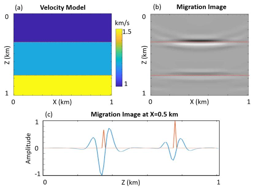
Figure 3: a) Three-layer velocity model, b) RTM image, and c) migration image (blue curve) at X=0.5 km, where the red curve is the normalized reflectivity model.

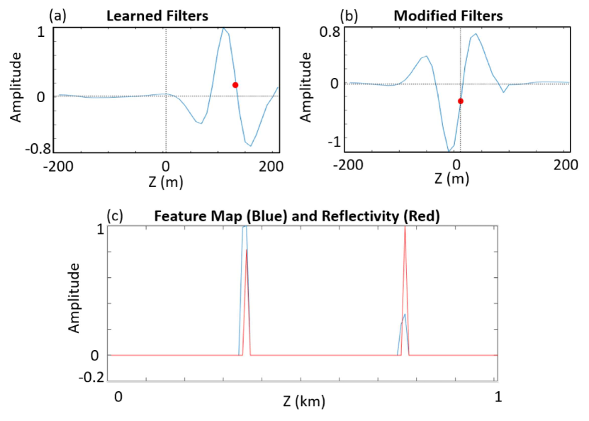
Figure 4: a) Learned filter, b) modified filter, and c) feature map (blue) and reflectivity model (red).

3.1 Three-layer Velocity Model

The interpretation of feature maps and filters can be understood by computing them for the Figure 3a model. The grid size of the model is 101$\times$101, and the grid interval is 10 m in both the x and z directions. There are 26 shots evenly spaced at a distance of 40 m on the surface, and each shot is recorded by 101 receivers with a sampling interval of 10 m. Figure 3b show the reverse time migration (RTM) image.

The first test is for a 1D model where we extract the image located at X$=0.5$ km, which is displayed as the blue curve in Figure 3c. The red curve in Figure 3c is the reflectivity model. Assume that there is only one filter in ${\bm{\Gamma}}$ and it extends over the depth of 400 m (41 grid points). We now compute the NNLSM image by finding the optimal ${\bf m}$ and ${\bm{\Gamma}}$ by the two-step iterative procedure denoted as the alternating descent method (see Liu and Schuster, (2018) and Liu et al., (2018)). The computed filter $\bm{\gamma}$_i is shown in Figure 4a where the phase of the filter ${\bm{\gamma}}_{i}$ is nonzero. If we use a filter with a non-zero time lag to calculate its feature map ${\bf m}$, the phases of the feature map and the true reflectivity ${\bf m}$ will be different. So, we need to modify the time lag and polarity of the basis function $\tilde{\bm{\Gamma}}_{i}$. The modified basis function is shown in Figure 4b, and its coefficients are displayed as the blue curve in Figure 4c. Compared with the true reflectivity ${\bf m}$ (red curve in Figure 4), the feature map can give the correct positions but also give the wrong values of the reflectivity distribution.

Next, we perform a 2D test where the input is the 2D migration image in Figure 3b. Three 35-by-35 (grid point) filters are learned (see Figure 5a). The modified filters are shown in Figure 5b. Appendix LABEL:D describes how we align the filters by using the cross-correlation method. The feature maps of these three filters are displayed in Figures 6a-6c. Figure 6d shows the sum of these three feature maps. It is evident that the stacked feature maps can estimate the correct locations of the reflectivity spikes.

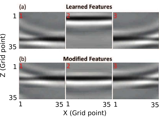
Figure 5: a) Learned and b) modified features.

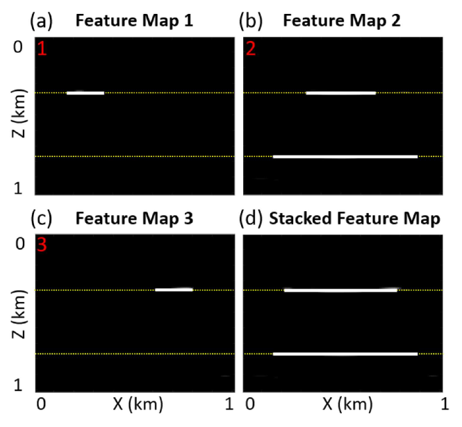
Figure 6: Feature maps for the features a) 1, b) 2, and c) 3 shown in Figure 5. The stacked feature map is shown in d). Here, the white lines show the locations of non-zero points and the yellow lines indicate the locations of the reflectivity distributions.

3.2 SEG/EAGE Salt Model

The multilayer NNLSM procedure (see equation 12) is now applied to the migration image associated with the 2D SEG/EAGE salt velocity model in Figure 7a. The grid size of the model is 101 grid points in both the z- and x-directions. The grid interval is 40 m in the x-direction and 20 m in the z-direction. Figure 7b shows the reverse time migration (RTM) image. The multilayer NNLSM consists of three convolutional layers: the first one contains 15 basis functions, i.e., filters, of size 11$\times$11 grid points, the second one consists of 15 basis functions with dimensions 11$\times$11$\times$15, and the last one contains contains 15 basis function of dimensions 11$\times$11$\times$15. Equation 12 is solved for both ${{\bf m}_{i}}$ and ${\bm{\Gamma}}_{i}$ ($i\in 1,2,3$) by the two-step iterative procedure denoted as the alternating descent method. The multilayered structure is shown in Figure 8, where the black dots in ${\bf m}_{i}$ represent the nonzero values of the quasi-reflectivity distribution. The effective basis functions computed for these layers are shown in Figures 7c-7e, where the yellow, red and green boxes indicate the sizes of the effective basis functions, which can be considered as quasi-migration Green’s functions. It indicates that the basis functions of the first layer ${\bm{\Gamma}}_{1}$ contain very simple small-dimensional edges, which are called “atoms” by Sulam et al., (2018). The non-zeros of the second group of basis functions ${\bm{\Gamma}}_{2}$ combine a few atoms from ${\bm{\Gamma}}_{1}$ to create slightly more complex edges, junctions and corners in the effective basis functions in ${\bm{\Gamma}}^{(2)}$. Lastly, ${\bm{\Gamma}}_{3}$ combines atoms from ${\bm{\Gamma}}^{(2)}$ in order to reconstruct the more complex parts of the migration image. The corresponding stacked coefficient images, also known as feature maps, are shown in Figures 7f-7h, which give the quasi-reflectivity distributions. The reconstructed migration images are shown in Figures 7i-7k.

For comparison, we computed the standard LSM image using the deblurring method described in Chen et al., (2017, 2019). Here, the deblurring filter size is 17x17 grid points (black boxes in Figure 9) and computed for a 50x50 grid (red boxes in Figure 9) of evenly spaced point scatterers with the same migration velocity model as used for the data migration in Figure 7a. The standard LSM images for the first and 50^th iterations are shown in Figures  10b and  10c, respectively, next to the NNLSM image in Figure 10d. It is clear that the NNLSM image is better resolved than the LSM image, although there are discontinuities in some of the NNLSM interfaces not seen in the LSM image. Some of the detailed geology is lost in the LSM image as seen in the wiggly interface in the red-rectangular area of Figure 10. The practical application of the NNLSM image is that it might serve a super-resolved attribute image that can be combined with other attributes to delineate geology. For example, combining the depth-slice of the NNLSM image with a spectral decomposition image (Aarre,, 2016) can help delineate the lithological edges of meandering channels.

NNLSM can filter out random and coherent noises in the migration image after reconstructing the migration image by eliminating the noisy learned basis functions and their coefficients in the NNLSM image. For example, Figure 11a shows the RTM image with a sparse acquisition geometry so that the image contains a strong acquisition footprint. The reconstructed migration image in Figure 11b shows significant mitigation of this noise in Figure 11a. However, the migration swing noise is still prominent near the red arrows in Figure 11b. Such noise is reconstructed from the noisy basis function shown in Figure 12a and the coefficients in Figure 12b. Figure 12c is the image reconstructed by correlating the basis function in Figure 12a with the coefficients in Figure 12b. After filtering out the basis functions from noise, the reconstructed image is shown in Figure 11c, which is free from aliasing noise at the locations indicated by the red arrows.

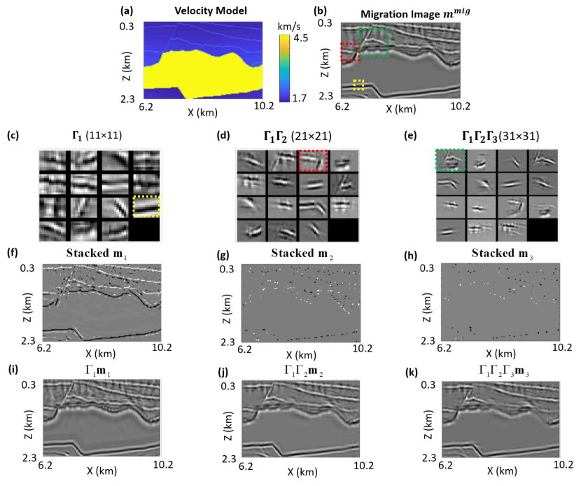
Figure 7: (a) 2D SEG/EAGE salt model, (b) RTM image, (c)-(e) learned effective filters ${\bm{\Gamma}}^{(1)}$, ${\bm{\Gamma}}^{(2)}$ and ${\bm{\Gamma}}^{(3)}$, (f)-(h) stacked quasi-reflectivity coefficients for ${\bf m}_{1}$, ${\bf m}_{2}$ and ${\bf m}_{3}$, (i)-(k) reconstructed migration images ${\bm{\Gamma}}^{(1)}{\bf m}_{1}$, ${\bm{\Gamma}}^{(2)}{\bf m}_{2}$ and ${\bm{\Gamma}}^{(3)}{\bf m}_{3}$.

Figure 8: Decomposition of the migration image of the 2D SEG/EAGE salt model in terms of the multi-layer filter $\bm{\Gamma}_{i}$ and pre-stacked quasi-reflectivity coefficient ${\bf m}_{i}$, where the black dots in ${\bf m}_{i}$ represent the nonzero value.

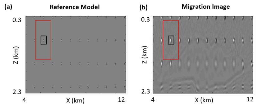
Figure 9: (a) Reference model and (b) its migration image for the standard deblurring LSM method.

Figure 10: (a) RTM image, (b) the first and (c) $50^{th}$ iteration results by LSM with deblurring, and (d) NNLSM image.

Figure 11: (a) RTM image, (b) reconstructed image with all basis functions, and (c) reconstructed image with selected basis functions.

Figure 12: (a) basis function from noise, (b) the coefficients, and (c) reconstructed image.

3.3 North Sea Data

Figure 13: a) Migration image computed from the F3 offshore block data, b) learned filters, c) stacked feature maps and d) migration image after filtering.

We apply the NNLSM method to field data collected in the North Sea (Schroot and Scüttenhelm,, 2003), where the time migration image is shown in Figure 13a. The time axis is gridded with 213 evenly-spaced points and there are 301 grid points along the x-axis. We compute 21 13-by-5 (grid point) convolutional basis functions, i.e. filters $\bm{\gamma}_{i}$ for ($i=1,2,...21$), by the NNLSM procedure (see Figure 13b). These filters approximate the dip-filtered migration Green’s functions, and the basis function is marked as the yellow boxes in Figure 13a and 13b. The stacked feature maps (quasi-reflectivity distribution) are displayed in Figure 13c. It is evident that the stacked feature maps can provide a high-resolution migration image. After reconstruction from the learned filters and feature maps, the migration image is shown in Figure 13d with less noise.

Finally, we apply NNLSM to a time slice of the migration image, which is shown in Figure 14a, and the image size is 301 by 301 gridpoints. Figure 14b shows the 21 13$\times$5 filters estimated by the NNLSM procedure. The stacked feature map is displayed in Figure 14c, which may be used as a superresolution attribute image for high-resolution delineation of geologic bodies. The reconstructed migration image is shown in Figure 14d and we can see there is less noise.

Figure 14: a) Time slice of the migration image computed from the F3 offshore block data, b) learned filters, c) stacked feature maps and d) migration image after filtering.

Figure 15: The relationship between sparse inversion and CNN, where the sparse inversion methods include sparse LSM, NNLSM, and blind deconvolution.

4 Discussion

The forward modeling for a multilayered neural network is shown to be equivalent to a single-iterate solution of a multilayered LSM problem. This assumes positivity and shrinkage constraints on the soft thresholding operation, so it reduces to the ReLu operation. This equivalence relates the physics of seismic imaging to architectural features in the neural network.

• The size of the filters in the first layer should be about the same size as the Green’s function for that model. Experiments with numerical models suggest that this size is approximately one-to-two wavelengths. In this case, the filter is interpreted as an approximation to the migration Green’s function, except it is that for a reflecting segment. Thus, we interpret the approximate migration Green’s function as a migration segment spread function (SSF) rather than a migration point spread function. Sulam et al., (2018) classifies each feature in the first layer as an atom which takes on the role of a SSF.

• The output of the first layer provides the small scale, i.e., high-wavenumber, features associated with the input data. For an input migration image, the feature maps of the first layer resemble sub-quasi-reflectivity maps of the subsurface. Adding the sub-quasi-reflectivity maps together gives a close approximation to the actual reflectivity model as shown in Figures 6d and 7f.

• The output of the second layer is a weighted sum of the first-layer features, which create sparser feature maps. Sulam et al., (2018) classifies the concatenation of the filters from the first and second layers as molecules (see equation 14). In the migration problem, the resulting filters are SSFs for even larger segments of the original reflector boundaries. The feature maps of the third layer are a weighted sum of the second layer’s features to produce even the sparsest feature maps. For migration, the final feature maps are very sparse while the concatenated filters are associated with large-scale features of the migration image.

• The computational cost of computing NNLSM images is significantly less than that for LSM images because no solutions of the wave equation are needed. For example, we consider the 2D FDTD forward modeling of the acoustic equation with an eighth-order scheme in space and a second-order scheme in time, and its computational complexity is $O(n_{t}n^{2})$ for one shot, where $n$ is the number of grid points in one direction and $n_{t}$ is the number of the time steps. According to Plessix, (2007), $n_{t}$ is approximate $30\ n$ to satisfy the stability condition and to make sure there is enough recoding time when $v_{max}/v_{min}\simeq=3$, where $v_{max}$ and $v_{min}$ are the maximum and minimum velocities, respectively. So, The complexity of 2D FDTD forward modeling of the acoustic equation is $O(n_{s}n^{3})$ where $n_{s}$ is the number of the shots. The complexity of LSRTM is $O(6n_{s}N^{iter}n^{3})$ (Schuster,, 2017), where $N^{iter}$ is the iteration number. For NNLSM, the complexity is $O(N^{iter}n^{2}\log n)$ according to Heide et al., (2015) and can be reduced to $O(N^{iter}n^{2})$ if a local block coordinate-descent algorithm is used (Zisselman et al.,, 2019).

The 1D NNLSM can be interpreted as a blind deconvolution (BD) problem in seismic data processing (Kaaresen and Taxt,, 1998; Bharadwaj et al.,, 2018). It can be seen in Figure 5 that the filter of NNLSM is the source wavelet of BD and the coefficients of NNLSM are the quasi-reflectivity coefficients of BD. However, NNLSM can have more than one filter and the filters can be 2D or 3D filters. We show the relationship between BD, sparse LSM, NNLSM, and CNN in Figure 15.

NNLSM is an unsupervised learning method. Compared to a supervised learning method, it does not heavily depend on the huge amount of training data. However, it may need human intervention for inspecting the quality of the quasi-reflectivity images and we need to align the filters to get more consistent quasi-reflectivity.

In Figure 14, we apply 2D NNLSM to a time slice of the 3D North Sea Data. The 2D NNLSM method can be extended to a 3D implementation to learn a set of 3D filters. Incorporating the third dimension of information from 3D filters will likely lead to a better continuity of the reflectors in Figure 14c. However, the computational cost will increase by more than a multiplicative factor of $n$.

5 Conclusion

Neural network least squares migration finds the optimal quasi-reflectivity distribution and quasi-migration-Green’s functions that minimize a sum of migration misfit and sparsity regularization functions. The advantages of NNLSM over standard LSM are that its computational cost is significantly less than that for LSM and it can be used for filtering both coherent and incoherent noise in migration images. A practical application of the NNLSM image is as an attribute map that provides superresolution imaging of the layer interfaces. This attribute image can be combined with other attributes to delineate both structure and lithology in depth/time slices of migration images. Its disadvantage is that the NNLSM quasi-reflectivity image is only an approximation to the actual reflectivity distribution.

A significant contribution of our work is that we show that the filters and feature maps of a multilayered CNN are analogous to the migration Green’s functions and reflectivity distributions. For the first time we now have a physical interpretation of the filters and feature maps in deep CNN in terms of the operators for seismic imaging. Such an understanding has the potential to lead to better architecture design of the network and extend its application to waveform inversion. In answer to Donoho’s plea for more rigor, NNLSM represents a step forward in establishing the mathematical foundation of CNN in the context of least squares migration.

6 Acknowledgements

The research reported in this publication was supported by the King Abdullah University of Science and Technology (KAUST) in Thuwal, Saudi Arabia. We are grateful to the sponsors of the Center for Subsurface Imaging and Modeling Consortium for their financial support. For computer time, this research used the resources of the Supercomputing Laboratory at KAUST and the IT Research Computing Group. We thank them for providing the computational resources required for carrying out this work.

Migration Green’s Function

Schuster and Hu, (2000) show that the poststack migration (Yilmaz,, 2001) image $m({\bf x})^{mig}$ in the frequency domain is computed by weighting each reflectivity value $m({\bf z})$ by $\Gamma({\bf x}|{\bf z})$ and integrating over the model-space coordinates ${\bf z}$:

$${\mbox{f}or}~{}{\bf x}\in D_{model}:~{}~{}~{}~{}m({\bf x})=$$

$$\eta\int_{D_{model}}d{\bf z}\overbrace{\int_{{\bf y}\in D_{data}}d{\bf y}\omega^{4}G({\bf x}|{\bf y})^{2*}G({\bf y}|{\bf z})^{2}}^{\Gamma({\bf x}|{\bf z})}m({\bf z}),$$ (16)

where $\eta$ represents terms such as the frequency variable raised to the 4th power. The migration Green’s function $\Gamma({\bf x}|{\bf z})$ is given by

$${\mbox{f}or}~{}{\bf x},{\bf z}\in D_{model}:~{}~{}~{}~{}\Gamma({\bf x}|{\bf z})=$$

$$\eta\int_{{\bf y}\in D_{data}}d{\bf y}\omega^{4}G({\bf x}|{\bf y})^{2*}G({\bf y}|{\bf z})^{2}.~{}~{}~{}~{}~{}~{}$$ (17)

Here we implicitly assume a normalized source wavelet in the frequency domain, and $D_{model}$ and $D_{data}$ represent the sets of coordinates in, respectively, the model and data spaces. The term $G({\bf x}^{\prime}|{\bf x})=e^{i\omega\tau_{xx^{\prime}}}/||{\bf x}-{\bf x}^{\prime}||$ is the Green’s function for a source at ${\bf x}$ and a receiver at ${\bf x}^{\prime}$ in a smoothly varying medium. The traveltime $\tau_{xx^{\prime}}$ is for a direct arrival to propagate from ${\bf x}$ to ${\bf x}^{\prime}$.

The physical interpretation of the kernel $\Gamma({\bf x}^{\prime}|{\bf x})$ is that it is the migration operator’s response at ${\bf x}^{\prime}$ to a point scatterer at ${\bf x}$, otherwise known as the MGF or the migration Green’s function (Schuster and Hu,, 2000). It is analogous to the point spread function (PSF) of an optical lens for a point light source at ${\bf x}$ in front of the lens and its optical image at ${\bf x}^{\prime}$ behind the lens on the image plane. In discrete form, the modeling term $[{\bm{\Gamma}{\bf m}}]_{i}$ in equation 16 can be expressed as

$$[{\bm{\Gamma}}{\bf m}]_{i} = \sum_{j}\Gamma({\bf x}_{i}|{\bf z}_{j})m_{j}.$$ (18)

with the physical interpretation that $[{\bm{\Gamma}}{\bf m}]_{i}$ is the migration Green’s function response at ${\bf x}_{i}$. An alternative interpretation is that $[{\bm{\Gamma}}{\bf m}]_{i}$ is the weighted sum of basis functions $\Gamma({\bf x}_{i}|{\bf z}_{j})$ where the weights are the reflection coefficients $m_{j}$ and the summation is over the $j$ index. We will now consider this last interpretation and redefine the problem as finding both the weights $m_{i}$ and the basis functions $\Gamma({\bf x}_{i}|{\bf z}_{j})$. This will be shown to be equivalent to the problem of a fully connected (FCN) neural network.

Soft Thresholding Function Define the sparse inversion problem as finding the optimal value $x^{*}$ that minimizes the objective function

$$\epsilon = \frac{1}{2}||{\bf z}-{\bf x}||_{2}^{2}+\lambda||{\bf x}||_{1},$$ (19)

where the $L_{1}$ norm demands sparsity in the solution ${\bf x}$. An example is where ${\bf z}$ is a noisy $M\times N$ image such that ${\bf z}={\bf x}+\mbox{noise}$, and we seek the optimal vector ${\bf x}$ that satisfies equation 19. Here, the noisy $M\times N$ image has been flattened into the tall $MN\times 1$ vector ${\bf z}$.

The stationary condition for equation 19 is

$$\frac{\partial\epsilon}{\partial x_{i}} = (x_{i}-z_{i})+\lambda\frac{\partial||{\bf x}||_{1}}{\partial x_{i}},$$ (20)

$$= 0,$$

where

$$\frac{\partial||{\bf x}||_{1}}{\partial x_{i}}=1~{}for~{}x_{i}\geq 0; \frac{\partial||{\bf x}||_{1}}{\partial x_{i}}=-1~{}for~{}x_{i}<0.$$ (21)

Equations 20-21 can be combined to give the optimal $x^{*}$ expressed as the two-sided ReLu function

$$x_{i}=\mbox{soft}(z_{i},\lambda)={\left\{\begin{array}[]{cl}z_{i}-\lambda&if~{}~{}z_{i}~{}~{}\geq~{}~{}\lambda\\ 0&if~{}~{}|z_{i}|<~{}~{}\lambda\\ z_{i}+\lambda&if~{}~{}z_{i}~{}~{}<-\lambda\end{array}\right\}}.$$ (22)

More generally, the iterative-soft-threshold-algorithm (ISTA) that finds ${\bf x}^{*}$

$${\bf x}^{*} = \arg\min_{{\bf x}}{\Big{[}}\frac{1}{2}||{\bf z}-{\bf W}{\bf x}||_{2}^{2}+\lambda||{\bf x}||_{1}{\Big{]}},$$ (23)

is

$$x_{i}^{(k+1)} = {\mbox{soft}}{\Big{(}}{\bf x}^{(k)}-\frac{1}{\alpha}{{\bf W}}^{T}({\bf W}{\bf x}^{(k)}-{\bf z}),\frac{\lambda}{\alpha}{\Big{)}}_{i}.$$ (24)

There are several more recently developed algorithms that have faster convergence properties than ISTA. For example, FISTA (Fast-ISTA) has quadratic convergence (Beck and Teboulle,, 2009). Neural Network Least Squares Migration

The neural network least squares migration (NNLSM) algorithm in the image domain is defined as solving for both the basis functions $\tilde{\Gamma}({\bf x}_{i}|{\bf x}_{j})$ and $\tilde{m}_{j}$ that minimize the objective function defined in equation 5. In contrast, SLSM only finds the least squares migration image in the image domain and uses the pre-computed migration Green’s functions that solve the wave equation.

The NNLSM solution is defined as

$$(\tilde{\bf m}^{*},\tilde{\bm{\Gamma}}^{*})=\arg\min_{\tilde{\bf m},~{}\tilde{\bm{\Gamma}}}{\Big{[}}\frac{1}{2}||\tilde{\bm{\Gamma}}\tilde{\bf m}-{\bf m}^{mig}||_{2}^{2}+\lambda S(\tilde{\bf m}){\Big{]}},$$ (25)

where now both $\tilde{\bm{\Gamma}}^{*}$ and $\tilde{\bf m}^{*}$ are to be found. The functions with tildes are mathematical constructs that are not necessarily identical to those based on the physics of wave propagation as in equation 5.

The explicit matrix-vector form of the objective function in equation 25 is given by

$$\epsilon=\frac{1}{2}\sum_{i}{\Big{[}}\sum_{j}\tilde{\Gamma}({\bf x}_{i}|{\bf z}_{j})\tilde{m}_{j}-m_{i}^{mig}{\Big{]}}^{2}+\lambda S(\tilde{\bf m}).$$ (26)

and its Fréchet derivative with respect to $\tilde{\Gamma}({\bf x}_{i^{\prime}}|{\bf z}_{j^{\prime}})$ is given by

$${\frac{\partial\epsilon}{\partial{\tilde{\Gamma}}({\bf x}_{i^{\prime}}|{\bf z}_{j^{\prime}})}} = \sum_{j}(\tilde{\Gamma}({\bf x}_{i^{\prime}}|{\bf z}_{j})\tilde{m}_{j}-\tilde{m}_{i^{\prime}}^{mig})\tilde{m}_{j^{\prime}}.$$ (27)

The iterative solution of equation 25 is given in two steps (Olshausen and Field,, 1996).

1. Iteratively estimate $\tilde{m}_{i}$ by the gradient descent formula used with SLSM:

   $$\tilde{m}_{i}^{(k+1)}=\tilde{m}_{i}^{(k)}-\alpha[\tilde{\bm{\Gamma}}^{T}(\tilde{\bm{\Gamma}}\tilde{\bf m}-{\bf m}^{mig})]_{i}-\lambda S(\tilde{\bf m})_{i}^{\prime}.$$ (28)

   However, one migration image ${\bf m}^{mig}$ is insufficient to find so many unknowns. In this case the original migration image is broken up into many small pieces so that there are many migration images to form examples from a large training set. For prestack migration, there will be many examples of prestack migration images, one for each shot, and the compressive sensing technique denoted as VISTA (Ahmad et al.,, 2015) is used for the calculations.

2. Update the basis functions $\tilde{\Gamma}({\bf x}_{i}|{\bf z}_{j})$ by inserting equation 27 into the gradient descent formula to get

   $$\tilde{\Gamma}({\bf x}_{i^{\prime}}|{\bf z}_{j^{\prime}})^{(k+1)}=\tilde{\Gamma}({\bf x}_{i^{\prime}}|{\bf z}_{j^{\prime}})^{(k+1)}-\alpha\frac{\partial\epsilon}{\partial{\tilde{\Gamma}}({\bf x}_{i^{\prime}}|{\bf z}_{j^{\prime}})},~{}~{}~{}~{}$$

   $$=\tilde{\Gamma}({\bf x}_{i^{\prime}}|{\bf z}_{j^{\prime}})^{(k+1)}$$

   $$-\alpha({\Big{\{}}\sum_{j}\tilde{\Gamma}({\bf x}_{i^{\prime}}|{\bf z}_{j})\tilde{m}_{j}{\Big{\}}}-m_{i^{\prime}}^{mig})\tilde{m}_{j^{\prime}}.$$ (29)

   It is tempting to think of $\tilde{\Gamma}({\bf x}|{\bf x}^{\prime})$ as the migration Green’s function and $\tilde{m}_{i}$ as the component of reflectivity. However, there is yet no justification to submit to this temptation and so we must consider, unlike in the SLSM algorithm, that $\tilde{\Gamma}({\bf x}|{\bf x}^{\prime})$ is a sparse basis function and $\tilde{m}_{i}$ is its coefficient. To get the true reflectivity then we should equate equation 18 to $\sum_{j}\tilde{\Gamma}({\bf x}_{i},{\bf x}_{j})\tilde{m}_{j}$ and solve for $m_{j}$.

Alignment of the Filters

To align the learned filters, we first choose a “target” filter, which is denoted as a 2D matrix ${\bf A}$ with the size of $M\times N$. Then we try to align all the other filters with the target filter through their cross-correlation. For example, if we choose one filter denoted as matrix ${\bf B}$ with the same size as ${\bf A}$, we can get the cross-correlation matrix $\bf C$ with its elements defined as,

$${C}_{i+M,j+N}=\sum_{m=1}^{M}\sum_{j=1}^{N}{a}_{m,n}\cdot{b}_{m+i,n+j},$$ (30)

where $-M<i<M$ and $-N<j<N$. $a_{i,j}$, $b_{i,j}$ and $C_{i,j}$ indicate the element at position $(i,j)$ in matrices $\bf A$, $\bf B$ and $\bf C$, respectively. The location of the maximum absolute value of the elements in matrix $\bf C$ indicates how much should we shift filter $\bf B$ to filter $\bf A$ in each direction. Figure 16 shows the calculation of the cross-correlation matrix $\bf C$ for two filters $A$ and $B$. $c_{1,0}$ (or $C_{4,3}$) is the maximum absolute value of the elements in matrix $\bf C$, which indicates filter $\bf B$ should be shifted 1 position along the first direction. Here, we need to pad zeros along all the dimensions of filter $\bf B$ before shifting it, which is displayed in Figure 17.

Figure 18a shows the learned filters with a size of $17\times 9$ from the migration image of the SEG/EAGE salt model. Filter No. 7 (yellow box) is chosen as the target filter. The aligned filters are shown in Figure 18b without zero padding and the stacked feature maps from the original and aligned filters are displayed in Figures 18c and 18d, respectively. It is evident that the reflector interfaces from the aligned filters are more continuous especially in the red box compared with those of the original filters.

Figure 16: Calculation of the cross-correlation matrix $\bf C$.

Figure 17: Diagram that illustrates the circular shifting of padded filter $\bf B$.

Figure 18: (a) Learned filters from the migration image of SEG/EAGE salt model; (b) the aligned filters; stacked feature maps of the (c) orginal and (d) aligned filters, where the yellow boxes show the sizes of the filters for the filters, respectively.

References

- Aarre, (2016) Aarre, V., 2016, Understanding spectral decomposition by victor aarre: https://youtu.be/1nDyMHs8zuw. (Accessed: 2019-04-19).
- Ahmad et al., (2015) Ahmad, R., H. Xue, S. Giri, Y. Ding, J. Craft, and O. P. Simonetti, 2015, Variable density incoherent spatiotemporal acquisition (VISTA) for highly accelerated cardiac MRI: Magnetic Resonance in Medicine, 74, no. 5, 1266–1278.
- Araya-Polo et al., (2018) Araya-Polo, M., J. Jennings, A. Adler, and T. Dahlke, 2018, Deep-learning tomography: The Leading Edge, 37, no. 1, 58–66.
- Bader et al., (2019) Bader, S., X. Wu, and S. Fomel, 2019, Missing log data interpolation and semiautomatic seismic well ties using data matching techniques: Interpretation, 7, no. 2, T347–T361.
- Beck and Teboulle, (2009) Beck, A., and M. Teboulle, 2009, A fast iterative shrinkage-thresholding algorithm for linear inverse problems: SIAM Journal on Imaging Sciences, 2, no. 1, 183–202.
- Bharadwaj et al., (2018) Bharadwaj, P., L. Demanet, and A. Fournier, 2018, Focused blind deconvolution of interferometric green’s functions: SEG Technical Program Expanded Abstracts 2018, 4085–4090.
- Cao and Roy, (2017) Cao, J., and B. Roy, 2017, Time-lapse reservoir property change estimation from seismic using machine learning: The Leading Edge, 36, no. 3, 234–238.
- Chavent and Plessix, (1999) Chavent, G., and R.-E. Plessix, 1999, An optimal true-amplitude least-squares prestack depth-migration operator: Geophysics, 64, no. 2, 508–515.
- Chen et al., (2017) Chen, Y., G. Dutta, W. Dai, and G. T. Schuster, 2017, Q-least-squares reverse time migration with viscoacoustic deblurring filters: Geophysics, 82, no. 6, S425–S438.
- Chen et al., (2019) Chen, Y., B. Guo, and G. T. Schuster, 2019, Migration of viscoacoustic data using acoustic reverse time migration with hybrid deblurring filters: Geophysics, 84, no. 3, S127–S136.
- De Roeck, (2002) De Roeck, Y.-H., 2002, Sparse linear algebra and geophysical migration: A review of direct and iterative methods: Numerical Algorithms, 29, no. 4, 283–322.
- Di et al., (2020) Di, H., Z. Li, H. Maniar, and A. Abubakar, 2020, Seismic stratigraphy interpretation by deep convolutional neural networks: A semi-supervised workflow: Geophysics, 85, no. 4, 1–41.
- Donoho, (2019) Donoho, D. L., 2019, Deepnet spectra and the two cultures of data science: Presented at the Al-Kindi Distinguished Statistics Lectures, KAUST.
- Duquet et al., (2000) Duquet, B., K. J. Marfurt, and J. A. Dellinger, 2000, Kirchhoff modeling, inversion for reflectivity, and subsurface illumination: Geophysics, 65, no. 4, 1195–1209.
- Dutta, (2017) Dutta, G., 2017, Sparse least-squares reverse time migration using seislets: Journal of Applied Geophysics, 136, 142–155.
- Feng and Schuster, (2017) Feng, Z., and G. T. Schuster, 2017, Elastic least-squares reverse time migration: Geophysics, 82, no. 2, S143–S157.
- Heide et al., (2015) Heide, F., W. Heidrich, and G. Wetzstein, 2015, Fast and flexible convolutional sparse coding: Proceedings of the IEEE Conference on Computer Vision and Pattern Recognition, 5135–5143.
- Herrmann et al., (2009) Herrmann, F. J., C. R. Brown, Y. A. Erlangga, and P. P. Moghaddam, 2009, Curvelet-based migration preconditioning and scaling: Geophysics, 74, no. 4, A41–A46.
- Hu et al., (2019) Hu, L., X. Zheng, Y. Duan, X. Yan, Y. Hu, and X. Zhang, 2019, First-arrival picking with a U-net convolutional network: Geophysics, 84, no. 6, U45–U57.
- Huang et al., (2017) Huang, L., X. Dong, and T. E. Clee, 2017, A scalable deep learning platform for identifying geologic features from seismic attributes: The Leading Edge, 36, no. 3, 249–256.
- Jia et al., (2018) Jia, Y., S. Yu, and J. Ma, 2018, Intelligent interpolation by monte carlo machine learning: Geophysics, 83, no. 2, V83–V97.
- Kaaresen and Taxt, (1998) Kaaresen, K. F., and T. Taxt, 1998, Multichannel blind deconvolution of seismic signals: Geophysics, 63, no. 6, 2093–2107.
- Karimpouli et al., (2010) Karimpouli, S., N. Fathianpour, and J. Roohi, 2010, A new approach to improve neural networks’ algorithm in permeability prediction of petroleum reservoirs using supervised committee machine neural network (SCMNN): Journal of Petroleum Science and Engineering, 73, no. 3-4, 227–232.
- Kaur et al., (2020) Kaur, H., N. Pham, and S. Fomel, 2020, Improving resolution of migrated images by approximating the inverse hessian using deep learning: Geophysics, Just accepted.
- Kühl and Sacchi, (2003) Kühl, H., and M. D. Sacchi, 2003, Least-squares wave-equation migration for AVP/AVA inversion: Geophysics, 68, no. 1, 262–273.
- Lailly, (1983) Lailly, P., 1983, The seismic inverse problem as a sequence of before stack migrations: Conference on inverse scattering: theory and application, Siam Philadelphia, PA, 206–220.
- Li and Gao, (2018) Li, F., and J. Gao, 2018, Sparse least-squares reverse time migration using 2-D undecimated wavelet transform: International Geophysical Conference, Beijing, China, 24-27 April 2018, Society of Exploration Geophysicists and Chinese Petroleum Society, 616–619.
- Liu et al., (2019) Liu, Z., J. Cao, Y. Lu, S. Chen, and J. Liu, 2019, A seismic facies classification method based on the convolutional neural network and the probabilistic framework for seismic attributes and spatial classification: Interpretation, 7, no. 3, SE225–SE236.
- Liu et al., (2018) Liu, Z., K. Lu, and X. Ge, 2018, Convolutional sparse coding for noise attenuation of seismic data: SEG 2018 Workshop: SEG Maximizing Asset Value Through Artificial Intelligence and Machine Learning, Beijing, China, 17–19 September 2018, 5–9.
- Liu and Schuster, (2018) Liu, Z., and G. Schuster, 2018, Neural network least squares migration: First EAGE/SBGf Workshop on Least-Squares Migration, Nov 2018, 1–5.
- Liu and Schuster, (2019) ——–, 2019, Multilayer sparse LSM = deep neural network: SEG Technical Program Expanded Abstracts 2019, 2323–2327.
- Lu and Feng, (2018) Lu, K., and S. Feng, 2018, Auto-windowed super-virtual interferometry via machine learning: A strategy of first-arrival traveltime automatic picking for noisy seismic data: SEG 2018 Workshop: SEG Maximizing Asset Value Through Artificial Intelligence and Machine Learning, Beijing, China, 17–19 September 2018, 10–14.
- Mandelli et al., (2018) Mandelli, S., F. Borra, V. Lipari, P. Bestagini, A. Sarti, and S. Tubaro, 2018, Seismic data interpolation through convolutional autoencoder: SEG Technical Program Expanded Abstracts 2018, Society of Exploration Geophysicists, 4101–4105.
- Mandelli et al., (2019) Mandelli, S., V. Lipari, P. Bestagini, and S. Tubaro, 2019, Interpolation and denoising of seismic data using convolutional neural networks: arXiv preprint arXiv:1901.07927.
- Nemeth et al., (1999) Nemeth, T., C. Wu, and G. T. Schuster, 1999, Least-squares migration of incomplete reflection data: Geophysics, 64, no. 1, 208–221.
- Olshausen and Field, (1996) Olshausen, B. A., and D. J. Field, 1996, Emergence of simple-cell receptive field properties by learning a sparse code for natural images: Nature, 381, no. 6583, 607.
- Papyan et al., (2016) Papyan, V., Y. Romano, and M. Elad, 2016, Convolutional neural networks analyzed via convolutional sparse coding: arXiv:1607.08194.
- (38) ——–, 2017a, Convolutional neural networks analyzed via convolutional sparse coding: The Journal of Machine Learning Research, 18, no. 1, 2887–2938.
- (39) Papyan, V., Y. Romano, J. Sulam, and M. Elad, 2017b, Convolutional dictionary learning via local processing: Proceedings of the IEEE International Conference on Computer Vision, 5296–5304.
- Perez et al., (2013) Perez, D. O., D. R. Velis, and M. D. Sacchi, 2013, Estimating sparse-spike attributes from ava data using a fast iterative shrinkage-thresholding algorithm and least squares, in SEG Technical Program Expanded Abstracts 2013: Society of Exploration Geophysicists, 3062–3067.
- (41) Peters, B., J. Granek, and E. Haber, 2019a, Multiresolution neural networks for tracking seismic horizons from few training images: Interpretation, 7, no. 3, SE201–SE213.
- (42) Peters, B., E. Haber, and J. Granek, 2019b, Neural networks for geophysicists and their application to seismic data interpretation: The Leading Edge, 38, no. 7, 534–540.
- Pham et al., (2020) Pham, N., X. Wu, and E. Zabihi Naeini, 2020, Missing well log prediction using convolutional long short-term memory network: Geophysics, 85, no. 4, 1–55.
- Plessix, (2007) Plessix, R.-E., 2007, A Helmholtz iterative solver for 3D seismic-imaging problems: Geophysics, 72, no. 5, SM185–SM194.
- Qian et al., (2018) Qian, F., M. Yin, X.-Y. Liu, Y.-J. Wang, C. Lu, and G.-M. Hu, 2018, Unsupervised seismic facies analysis via deep convolutional autoencoders: Geophysics, 83, no. 3, A39–A43.
- Richardson, (2018) Richardson, A., 2018, Seismic full-waveform inversion using deep learning tools and techniques: arXiv preprint arXiv:1801.07232.
- Rolon et al., (2009) Rolon, L., S. D. Mohaghegh, S. Ameri, R. Gaskari, and B. McDaniel, 2009, Using artificial neural networks to generate synthetic well logs: Journal of Natural Gas Science and Engineering, 1, no. 4-5, 118–133.
- Ross and Cole, (2017) Ross, C. P., and D. M. Cole, 2017, A comparison of popular neural network facies-classification schemes: The Leading Edge, 36, no. 4, 340–349.
- Sacchi and Ulrych, (1995) Sacchi, M. D., and T. J. Ulrych, 1995, High-resolution velocity gathers and offset space reconstruction: Geophysics, 60, no. 4, 1169–1177.
- Saggaf and Nebrija, (2003) Saggaf, M., and E. L. Nebrija, 2003, Estimation of missing logs by regularized neural networks: AAPG bulletin, 87, no. 8, 1377–1389.
- Salehi et al., (2017) Salehi, M. M., M. Rahmati, M. Karimnezhad, and P. Omidvar, 2017, Estimation of the non records logs from existing logs using artificial neural networks: Egyptian Journal of Petroleum, 26, no. 4, 957–968.
- Schroot and Scüttenhelm, (2003) Schroot, B., and R. Scüttenhelm, 2003, Expressions of shallow gas in the Netherlands North Sea: Netherlands Journal of Geosciences - Geologie en Mijnbouw, 82, no. 1, 91–105.
- Schuster and Liu, (2019) Schuster, G., and Z. Liu, 2019, Least squares migration: Current and future directions: 81st EAGE Conference and Exhibition 2019, European Association of Geoscientists & Engineers, 1–5.
- Schuster, (1993) Schuster, G. T., 1993, Least-squares cross-well migration, in SEG Technical Program Expanded Abstracts 1993: Society of Exploration Geophysicists, 110–113.
- Schuster, (2017) ——–, 2017, Seismic inversion: Society of Exploration Geophysicists.
- Schuster and Hu, (2000) Schuster, G. T., and J. Hu, 2000, Green’s function for migration: Continuous recording geometry: Geophysics, 65, no. 1, 167–175.
- Shi et al., (2019) Shi, Y., X. Wu, and S. Fomel, 2019, Saltseg: Automatic 3D salt segmentation using a deep convolutional neural network: Interpretation, 7, no. 3, SE113–SE122.
- Shi et al., (2020) ——–, 2020, Waveform embedding: automatic horizon picking with unsupervised deep learning: Geophysics, 85, no. 4, 1–48.
- Siahkoohi et al., (2018) Siahkoohi, A., R. Kumar, and F. Herrmann, 2018, Seismic data reconstruction with generative adversarial networks: 80th EAGE Conference and Exhibition 2018, European Association of Geoscientists & Engineers, 1–5.
- Sulam et al., (2018) Sulam, J., V. Papyan, Y. Romano, and M. Elad, 2018, Multilayer convolutional sparse modeling: Pursuit and dictionary learning: IEEE Transactions on Signal Processing, 66, no. 15, 4090–4104.
- Sun et al., (2020) Sun, J., Z. Niu, K. A. Innanen, J. Li, and D. O. Trad, 2020, A theory-guided deep-learning formulation and optimization of seismic waveform inversion: Geophysics, 85, no. 2, R87–R99.
- Tarantola, (1987) Tarantola, A., 1987, Inverse problem theory: Methods for data fitting and model parameter estimation: Elsevier.
- Waldeland et al., (2018) Waldeland, A. U., A. C. Jensen, L.-J. Gelius, and A. H. S. Solberg, 2018, Convolutional neural networks for automated seismic interpretation: The Leading Edge, 37, no. 7, 529–537.
- Wang et al., (2019) Wang, B., N. Zhang, W. Lu, and J. Wang, 2019, Deep-learning-based seismic data interpolation: A preliminary result: Geophysics, 84, no. 1, V11–V20.
- Wang and Sacchi, (2005) Wang, J., and M. D. Sacchi, 2005, Sparse regularization for least-squares AVP migration: CSEG National Convention, Expanded Abstracts, 117–120.
- Wang and Sacchi, (2007) ——–, 2007, High-resolution wave-equation amplitude-variation-with-ray-parameter (AVP) imaging with sparseness constraints: Geophysics, 72, no. 1, S11–S18.
- Wang et al., (2020) Wang, Y., B. Wang, N. Tu, and J. Geng, 2020, Seismic trace interpolation for irregularly spatial sampled data using convolutional autoencoder: Geophysics, 85, no. 2, V119–V130.
- Witte et al., (2017) Witte, P., M. Yang, and F. Herrmann, 2017, Sparsity-promoting least-squares migration with the linearized inverse scattering imaging condition: 79th EAGE Conference and Exhibition 2017, European Association of Geoscientists & Engineers, 1–5.
- (69) Wu, X., L. Liang, Y. Shi, Z. Geng, and S. Fomel, 2019a, Multitask learning for local seismic image processing: fault detection, structure-oriented smoothing with edge-preserving, and seismic normal estimation by using a single convolutional neural network: Geophysical Journal International, 219, no. 3, 2097–2109.
- (70) Wu, X., Y. Shi, S. Fomel, L. Liang, Q. Zhang, and A. Yusifov, 2019b, Faultnet3D: Predicting fault probabilities, strikes, and dips with a single convolutional neural network: IEEE Transactions on Geoscience and Remote Sensing, 57, 9138–9155.
- Xiong et al., (2018) Xiong, W., X. Ji, Y. Ma, Y. Wang, N. M. AlBinHassan, M. N. Ali, and Y. Luo, 2018, Seismic fault detection with convolutional neural network: Geophysics, 83, no. 5, O97–O103.
- Xu et al., (2019) Xu, Y., J. Li, and X. Chen, 2019, Physics informed neural networks for velocity inversion: SEG Technical Program Expanded Abstracts 2019, 2584–2588.
- Yilmaz, (2001) Yilmaz, Ö., 2001, Seismic data analysis: Processing, inversion, and interpretation of seismic data: Society of Exploration Geophysicists.
- Yuan et al., (2018) Yuan, S., J. Liu, S. Wang, T. Wang, and P. Shi, 2018, Seismic waveform classification and first-break picking using convolution neural networks: IEEE Geoscience and Remote Sensing Letters, 15, no. 2, 272–276.
- Zheng et al., (2019) Zheng, Y., Q. Zhang, A. Yusifov, and Y. Shi, 2019, Applications of supervised deep learning for seismic interpretation and inversion: The Leading Edge, 38, no. 7, 526–533.
- Zhu et al., (2017) Zhu, L., C. Zhang, Y. Wei, X. Zhou, Y. Huang, and C. Zhang, 2017, Inversion of the permeability of a tight gas reservoir with the combination of a deep boltzmann kernel extreme learning machine and nuclear magnetic resonance logging transverse relaxation time spectrum data: Interpretation, 5, no. 3, T341–T350.
- Zisselman et al., (2019) Zisselman, E., J. Sulam, and M. Elad, 2019, A local block coordinate descent algorithm for the CSC model: Proceedings of the IEEE Conference on Computer Vision and Pattern Recognition, 8208–8217.