Abstract

This paper is devoted to the multivariate estimation of a vector of Poisson means. A novel loss function that penalises bad estimates of each of the parameters and the sum (or equivalently the mean) of the parameters is introduced. Under this loss function, a class of minimax estimators that uniformly dominate the maximum likelihood estimator is derived. Crucially, these methods have the property that for estimating a given component parameter, the full data vector is utilised. Estimators in this class can be fine-tuned to limit shrinkage away from the maximum likelihood estimator, thereby avoiding implausible estimates of the sum of the parameters. Further light is shed on this new class of estimators by showing that it can be derived by Bayesian and empirical Bayesian methods. In particular, we exhibit a generalisation of the Clevenson–Zidek estimator, and prove its admissibility. Moreover, a class of prior distributions for which the Bayes estimators uniformly dominate the maximum likelihood estimator under the new loss function is derived. A section is included involving weighted loss functions, notably also leading to a procedure improving uniformly on the maximum likelihood method in an infinite-dimensional setup. Importantly, some of our methods lead to constructions of new multivariate models for both rate parameters and count observations. Finally, estimators that shrink the usual estimators towards a data based point in the parameter space are derived and compared.

Key words: admissibility; Bayes and empirical Bayes; minimax; Poisson; shrinkage; multivariate estimation

1   Introduction

Let $Y=(Y_{1},\ldots,Y_{p})$ be a vector of independent Poisson random variables with mean vector $\theta=(\theta_{1},\ldots,\theta_{p})$. In this article we consider the problem of estimating the vector $\theta$. The obvious estimator is $\delta_{0}(Y)=Y$, that is, using $\delta_{0,i}=Y_{i}$ for each of the $p$ individual parameters. It is well known that $\delta_{0}$ is the maximum likelihood solution, that it has components with uniformly minimal variance among the unbiased estimators, and that it is admissible in the one-dimensional problem under squared error loss as well as under its weighted version, see e.g. Lehmann (1983, p. 277). In the simultaneous or multivariate problem, however, Peng (1975) and Clevenson & Zidek (1975) were the first to show that $\delta_{0}$ can be improved upon under the loss functions

$$L_{0}^{*}(\theta,\delta)=\sum_{i=1}^{p}(\delta_{i}-\theta_{i})^{2}\quad{\rm and}\quad L_{1}^{*}(\theta,\delta)=\sum_{i=1}^{p}(\delta_{i}-\theta_{i})^{2}/\theta_{i},$$ (1.1)

if $p\geq 3$ and $p\geq 2$, respectively. In particular, for the $L_{1}^{*}$ loss, Clevenson & Zidek (1975) derived the estimator

$$\delta_{\text{CZ},i}(Y)=\Bigl{(}1-\frac{p-1}{p-1+Z}\Bigr{)}Y_{i},\quad{\rm where\ }Z=\sum_{i=1}^{p}Y_{i},$$ (1.2)

demonstrating that it improves uniformly on the standard procedure $\delta_{0}$. This Stein-type phenomenon has also been observed for other loss functions. Hwang (1982) obtained results for $\sum_{i=1}^{p}(\delta_{i}-\theta)^{2}/\theta_{i}^{m_{i}}$, for fixed integers $m_{i}$. Ghosh & Yang (1988) considered a loss function based on the entropy or Kullback–Leibler distance $L_{e}(\theta,\delta)=\sum_{i=1}^{p}\theta_{i}\{\delta_{i}/\theta_{i}-\log(\delta_{i}/\theta_{i})-1\}$, A good overview article for admissibility issues, for multivariate Poisson means and for other models for discrete data, is Ghosh, Hwang & Tsui (1983), followed by discussion contributions by Berger (1983), Morris (1983), Hudson (1983). A more recent article on these issues is Brown, Greenshtein & Ritov (2013).

More broadly, the books Efron (2013) and Fourdrinier, Strawderman & Wells (2018) contribute to seeing multivariate estimation, using shrinkage and empirical Bayes methods, as as a global phenomenon. Central themes are variations on ‘borrowing strength’, either via direct constructions or in empirical Bayes setups. Our article is a contribution in these general directions, showing that methods developed for the multinormal and more generally spherically symmetric distributions have certain parallels in the world of multivariate Poisson estimation. Importantly, when estimating a particular Poisson parameter $\theta_{i}$, the full multivariate vector of data is being used, as an integral part of our methods.

The estimators that have been found to be better than $\delta_{0}(Y)=Y$ in these earlier publications are essentially all of the shrinking type, pushing the maximum likelihood estimator closer to the bottom corner of the parameter space. A good example of the merits of this type of shrinkage is provided by Clevenson & Zidek (1975), wherein 36 small $\theta_{i}$ – intensities of an oil-well discovery process – are estimated with the estimator in (1.2). Clevenson & Zidek (1975) had access to ‘known’ $\theta_{i}$ and could check the actual loss incurred. The procedure in (1.2) did indeed give much smaller loss $\sum_{i=1}^{36}(\delta_{\text{CZ},i}-\theta_{i})^{2}/\theta_{i}$ than did $\delta_{0}$; the losses are 14.33 and 39.26, respectively. However, another and perhaps not so pleasant feature of their estimation procedure is conspicuous here, namely that the sum $\gamma=\sum_{i=1}^{36}\theta_{i}$ (or equivalently the mean $\bar{\theta}=\gamma/36$) is seriously underestimated. In their oil-well discovery example the true sum is $\gamma=26.98$, the usual $\delta_{0}$ has $\sum_{i=1}^{36}y_{i}=29$, while their $\sum_{i=1}^{36}\delta_{\text{CZ},i}=12.97$ is much too low.

In some situations the sum (or mean) is unimportant and all that matters is to estimate each $\theta_{i}$. In many multiparameter cases on wants to keep track of the sum (or the mean) of the $\theta_{i}$ as well, however, as one surely would in the oil-well discovery process above. Other multiparameter cases where the sum (or the mean) are deemed as important as the individual $\theta_{i}$ abound; think for example of a decision maker having to make budgetary decisions concerning each of the boroughs of a city and the city as a whole, the resources allocated to each of $p$ hospitals and the whole health budget, etc.

These considerations motivate studying loss functions that take into account the need for good individual estimates, while at the same time guarding against the underestimation of the sum. One example of such a loss function is

$$L(\theta,\delta)=\sum_{i=1}^{p}(\delta_{i}-\theta_{i})^{2}+c\Bigl{(}\sum_{i=1}^{p}\delta_{i}-\gamma\Bigr{)}^{2}=L_{0}^{*}(\theta,\delta)+cp^{2}(\bar{\delta}-\bar{\theta})^{2},$$ (1.3)

Since $\sum_{i=1}^{p}\delta_{0,i}=\sum_{i=1}^{p}Y_{i}$ is the admissible minimax solution under the loss function $\big{(}\sum_{i=1}^{p}\delta_{i}-\gamma\big{)}^{2}$ one might wonder whether the extra penalisation above would secure admissibility of $\delta_{0}$ in the simultaneous problem. In Section 2 we show that this is not the case; $\delta_{0}$ is again inadmissible when $p\geq 3$, under any given quadratic form loss function $(\delta-\theta)^{\rm t}A(\delta-\theta)$. Another loss function that takes the guarding against underestimation of the sum (or the mean) of the parameters into account is the weighted version of (1.3), that is, the loss functions that generalises the one used by Clevenson & Zidek (1975), namely

$$\begin{split}L_{c}(\theta,\delta)=\sum_{i=1}^{p}\frac{(\delta_{i}-\theta_{i})^{2}}{\theta_{i}}+c{(\sum_{i=1}^{p}\delta_{i}-\sum_{i=1}^{p}\theta_{i})^{2}\over\sum_{i=1}^{p}\theta_{i}}=L_{1}^{*}(\theta,\delta)+cp\frac{(\bar{\delta}-\bar{\theta})^{2}}{\bar{\theta}},\end{split}$$ (1.4)

where $c$ is a user-defined constant. Under (1.4), the loss in Clevenson and Zidek’s example for $\delta_{0}$ is $39.26+0.35\,c$ while the loss for $\delta_{\text{CZ}}$ is $14.33+6.35\,c$. Again, one might wonder whether $\delta_{0}$ is admissible for certain values of $c$. In Section 3 we show that this is not the case, and derive an estimator which is the natural generalisation of the one in (1.2),

$$\delta_{i}^{c}(Y)=\Bigl{\{}1-\frac{p-1}{p-1+(1+c)Z}\Bigr{\}}\,Y_{i}\quad{\rm for\ }i=1,\ldots,p,$$ (1.5)

which is shown to belong to a class of estimators that dominate $\delta_{0}$ uniformly over the parameter space. In the somewhat similar multivariate normal setting, investigations on how to limit the shrinkage of the James–Stein estimator, in order to account for objectives related to estimation the means, have been conducted by Efron & Morris (1971, 1972).

Our paper proceeds as follows. In Section 2 we study the loss function (1.3) and derive a class of estimators that uniformly dominate the maximum likelihood estimator. Section 3 concerns the weighted version of this loss function, the $L_{c}$ loss function of (1.4), and we derive the already mentioned generalisation $\delta^{c}$ of $\delta_{\rm CZ}$. In Section 4 further light is shed on this new class of estimators by showing that it can be derived by Bayesian and empirical Bayesian methods. We are also able to prove that the estimator $\delta^{c}$ of (1.5) is admissible. Classes of alternative estimators are then studied in Sections 5 and 6, involving Bayes and empirical Bayes strategies which shrink the raw data towards data-driven structures for the $\theta_{i}$, such as the data mean, or a submodel. Some of these procedures succeed in having risks well below the minimax benchmark, in large regions of the parameter space, though without achieving uniform dominance. In Section 7 weighted loss functions are studied, which admit relative weights of importance; notably, an infinite-dimensional setup is also included. Then in Section 8 we demonstrate how some of our Bayesian constructions also lead to new multivariate models for rate parameters and for count observations, of interest in their own right, pointing to models for spatially dependent count data. Finally Section 9 offers a list of concluding remarks.

2   General quadratic loss function

We may write the loss function of (1.3) as $L(\delta,\theta)=(\delta-\theta)^{\rm t}A_{0}(\delta-\theta)$, where $A_{0}$ is the matrix with $1+c$ down its diagonal and $c$ elsewhere. The natural generalisation is

$$L(\delta,\theta)=(\delta-\theta)^{\rm t}A(\delta-\theta),$$ (2.1)

where $A$ is symmetric and positive definite. Below we obtain some results for general $A$ and apply these to two examples. Note that in situations where there is no ordering of the individual $\theta_{i}$ and no reason to estimate some of them more precisely than the others, the loss function in (1.3), that is, using $A_{0}$ with an appropriate choice of $c$, is the natural choice. Our method of proving inadmissibility of $\delta_{0}$ resembles that of Tsui & Press (1982) and Hwang (1982), where $A$ is diagonal.

Let $\delta(y)=y-\phi(y)$ be a competitor. The difference in risk between these two estimators is then

$$\begin{split}R(\delta,\theta)-R(\delta_{0},\theta)&={\rm E}_{\theta}\,\{(\delta-\theta)^{\rm t}A(\delta-\theta)-(Y-\theta)^{\rm t}A(Y-\theta)\}\\ &={\rm E}_{\theta}\,\{-2(Y-\theta)A\phi(Y)+\phi(Y)^{\rm t}A\phi(Y)\}\\ &={\rm E}_{\theta}\,\{-2(Y-\theta)\psi(Y)+\psi(Y)^{\rm t}A^{-1}\psi(Y)\},\end{split}$$ (2.2)

writing $\psi(y)=A\phi(y)$. Furthermore, since ${\rm E}_{\theta}\,\theta_{i}g(Y)={\rm E}_{\theta}\,Y_{i}g(Y-e_{i})$ for any $g$ with ${\rm E}_{\theta}\,|g(Y)|<\infty$, using $e_{i}$ to denote the unit vector with the $i$th element equal to one, we have that

$${\rm E}_{\theta}\,(Y_{i}-\theta_{i})\psi(Y)={\rm E}_{\theta}\,Y_{i}\{\psi(Y)-\psi(Y-e_{i})\},$$

and the risk difference (2.2) can be written ${\rm E}_{\theta}\,D(Y,\phi)$, in which

$$D(y,\phi)=-\sum_{i=1}^{p}2y_{i}\{\psi(y)-\psi(y-e_{i})\}+\psi(y)^{\rm t}A^{-1}\psi(y).$$

If a function $\psi(y)$ can be found such that $D(y,\phi)$ is non-positive for all $y$, with strict inequality for at least one datum $y$, then $\delta_{0}=Y$ is inadmissible, being outperformed by $\delta(y)=y-A^{-1}\psi(y)$.

Theorem 1.

Let $A$ be symmetric and positive definite. Then $\delta_{0}=Y$ is inadmissible under loss function (2.1), if $p\geq 3$. It is dominated by $\delta(Y)=Y-A^{-1}\psi(Y)$, where $\psi(\cdot)$ is any member of the following class

$$\psi_{i}(y)=\frac{d(y)}{B(y)}T(y_{i}),\quad\text{for\ }i=1,\ldots p,$$

where $T(0)=0$ and $T(y)=\sum_{j\leq y}1/j$ for $y\geq 1$, where $B(y)=\sum_{i=1}^{p}T(y_{i})T(y_{i}+1)$, and $d(y)$ is nondecreasing in each argument and obeying

$$0\leq d(y)\leq(2/M)\{N(y)-2\}_{+},$$

writing $a_{+}=\max(a,0)$ for truncating to zero. Here $N(y)=\sum_{i=1}^{p}I\{y_{i}\leq 1\}$ and $M$ is the inverse of the smallest eigenvalue of $A$.

Proof.

The choice of $M$ entails $\psi^{\rm t}A^{-1}\psi\leq M\sum_{i=1}^{p}\psi_{i}^{2}$ so that

$$D(\phi,y)\leq-2\sum_{i=1}^{p}y_{i}\big{\{}\psi_{i}(y)-\psi_{i}(y-e_{i})\big{\}}+\sum_{i=1}^{p}M\psi_{i}(y)^{2}.$$

The general Theorem 2.1 in Hwang (1982), with accompanying corollaries, can then be used to find $\psi_{i}(\cdot)$ functions that make $D(\phi,y)$ non-positive for all $y$. We skip details but record that Hwang’s method gives

$$D(\phi,y)\leq-2d(y)\frac{\big{\{}N(y)-2-Md(y)/2\big{\}}_{+}}{B(y)},$$ (2.3)

which is non-positive for each $\psi(\cdot)$ described in the theorem. ∎

A natural choice for $d(y)$ is the following, minimising the upper bound in (2.3),

$$d_{0}(y)=(1/M)\{N(y)-2\}_{+}.$$

This means using $\phi_{0}(y)=A^{-1}\psi_{0}(y)$ with $D(\phi_{0},y)\leq-M^{-1}\{N(y)-2\}^{2}/B(y)$, which shows that

$$\delta(y)=y-A^{-1}\psi_{0}(y),\;\;\text{where}\;\;\psi_{0,i}(y)=\frac{1}{M}\frac{T(y_{i})}{B(x)}\{N(y)-2\}_{+},$$

achieves

$$R(\delta,\theta)-R(Y,\theta)\leq-M^{-1}{\rm E}_{\theta}\,\big{\{}(N(Y)-2)_{+}\big{\}}^{2}/B(Y)<0,$$

for all $\theta$. Note in particular that the same $\psi_{0}(\cdot)$ function works for a large class of loss function (2.1).

Example 2.1.

Let $A$ be the square matrix with $1+c$ down its diagonal and $c$ elsewhere. This matrix might be written $A=I+cee^{\rm t}$, with $I$ the identity matrix and $e=(1,\ldots,1)^{\rm t}$ the $p\times 1$ vector of ones. This choice of $A$ gives the loss function (1.3). Here $M=1$ and $A^{-1}=I-\{c/(1+cp)\}ee^{\rm t}$, and $\psi^{\rm t}A^{-1}\psi\leq\sum_{i=1}^{p}\psi_{i}^{2}$ follows. The natural estimator is then $\delta(y)=y-\phi_{0}(y)$, where

$$\phi_{0}(y)=\psi_{i,0}(y)-\frac{c}{1+cp}\sum_{j=1}^{p}\psi_{0,j}(y)=\{N(y)-2\}_{+}\frac{T(y_{i})-\frac{cp}{1+cp}\bar{T}(y)}{B(y)},$$

in which $\bar{T}(y)=p^{-1}\sum_{i=1}^{p}T(y_{i})$. Note that $\delta$ does not shrink the $y$ in any particular direction, but rather pushes the components $y_{i}$ in different directions according to the sign of $T(y_{i})-\{cp/(1+cp)\}\bar{T}(y)$. Note further that if the $y_{i}$ are moderate or large, then

$$\delta_{i}(y)\doteq y_{i}-{p-2\over\sum_{j=1}^{p}(\log y_{j})^{2}}\Bigl{\{}\log y_{i}-{cp\over 1+cp}{1\over p}\sum_{j=1}^{p}\log y_{j}\Bigr{\}}.$$

Example 2.2.

Samples of independent Poisson variables arise naturally when one or more Poisson processes are observed over time. Dividing the time interval into $p$ parts gives counts $y_{1},\ldots,y_{p}$ with certain means $\theta_{1},\ldots,\theta_{p}$. In the nonparametric setting, where the intensity of the process is unknown, these parameters are also completely unknown. If one wishes to estimate the cumulative intensity of the process, then $(\lambda_{1},\ldots,\lambda_{p})$ are more important than $(\theta_{1},\ldots,\theta_{p})$, where $\lambda_{i}=\sum_{j=1}^{i}\theta_{j}$. This suggests using the loss function $L(\theta,\delta)=\sum_{i=1}^{p}(\widehat{\lambda}_{i}-\lambda_{i})^{2}$, where $\widehat{\lambda}_{i}=\sum_{j=1}^{i}\delta_{j}$. But this is seen to be a special case of (2.1), with elements $a_{i,j}=p+1-\max(i,j)$ filling the $A$ matrix. Its inverse $A^{-1}$ has first row $(1,-1,0,\ldots,0)$, last row $(0,\ldots,0,-1,2)$, and in between we find $(0,\ldots,0,-1,2,-1,0,\ldots,0)$. One has $\psi^{\rm t}A^{-1}\psi\leq 4\psi^{\rm t}\psi$, and can use $M=4$ when applying the theorem. Hence the following estimator improves on $\delta_{0}=Y$:

$$\delta_{1}^{*}(y) = y_{1}-\psi_{0,1}(y)+\psi_{0,2}(y),$$

$$\delta_{i}^{*}(y) = y_{i}+\psi_{0,i-1}(y)-2\psi_{0,i}(y)+\psi_{0,i+1}(y)\quad{\rm for\ }2\leq i\leq p-1,$$

$$\delta_{p}^{*}(y) = y_{p}+\psi_{0,p-1}(y)-2\psi_{0,p}(y),$$

where this time

$$\psi_{0,i}(y)={1\over 4}{T(y_{i})\over B(y)}\{N(y)-2\}_{+}.$$

Notice finally that the corresponding improved estimators for the cumulative $\lambda_{i}$ become

$$\widehat{\lambda}_{i}=\sum_{j=1}^{i}Y_{j}-\psi_{0,i}(Y)+\psi_{0,i+1}(Y)\quad{\rm for\ }i\leq p-1,$$

while $\widehat{\lambda}_{p}=\sum_{j=1}^{p}Y_{j}-\psi_{0,p}(Y)$.

3   The $L_{c}$ loss function

The main consideration leading to the loss function $(\delta_{i}-\theta_{i})^{2}/\theta_{i}$ is that the statistician seeks precise estimates of small values of $\theta_{i}$. A loss function that penalises heavily for bad estimates of small parameters is then a natural choice. Related to this is the obvious fact that when the parameters are small, they can only be badly overestimated, zero being the boundary of the parameter space. The corresponding multiparameter version of this is $\sum_{i=1}^{p}(\delta_{i}-\theta_{i})^{2}/\theta_{i}$, and is the one treated by Ghosh, Hwang & Tsui (1983), Hwang (1982), Tsui & Press (1982), Clevenson & Zidek (1975), and others. Note that $\delta_{0}=Y$ has constant risk $p$ with this loss, and it is not difficult to establish that it is minimax.

The above mentioned authors obtain classes of estimators that perform uniformly better than $\delta_{0}$ if only $p\geq 2$. As discussed in Section 1 and illustrated by the oil-well example, these shrinkage estimators do not take into account the additional desideratum, namely a precise estimate of the sum $\gamma=\sum_{i=1}^{p}\theta_{i}$. We will now study the $L_{c}$ loss function of (1.4), $L_{c}(\theta,\delta)=L_{1}^{*}(\theta,\delta)+c(\sum_{i=1}^{p}\delta_{i}-\gamma)^{2}/\gamma$. If we consider the second term in (1.4) by itself, we recognise the one-dimensional loss function $(\delta-\gamma)^{2}/\gamma$. It is well known that $\widehat{\gamma}=Z$ is admissible and the unique minimax solution under this loss function, and can therefore not be uniformly improved upon (Lehmann, 1983, p. 277). Consequently, since $z$ is the sum of the $y_{i}$, higher values of $c$ will result in estimators that lie closer the $\delta_{0}$. On the other hand, we know that for $c=0$ the estimator in (1.2) uniformly dominates $\delta_{0}$. Hence, the user defined constant $c$ determines how to compromise between $\delta_{0}$ and $\delta_{\text{CZ}}$.

Before we derive a class of estimators that dominate $\delta_{0}$ under $L_{c}$ in Section 3.2, we derive formulae for the Bayes solution and show that $\delta_{0}$ is minimax.

3.1   The $\delta_{0}=Y$ estimator is minimax.

The maximum likelihood estimator $\delta_{0}=Y$ has constant risk $p+c$ under $L_{c}$ and is a natural candidate for being minimax. We demonstrate minimaxity by exhibiting a sequence of priors with minimum Bayes risks $\text{BR}(\delta,\pi)={\rm E}\,R_{c}(\delta,\theta)$ which converge towards $p+c$; that this is sufficient follows from well-known arguments, as exposited e.g. in Robert (2007, Ch. 2.4). Some analysis is required to characterise the Bayes solution. We first find the values $\delta_{1},\ldots,\delta_{p}$ that minimise the posterior expected loss, i.e. given a dataset $y=(y_{1},\ldots,y_{p})$, with respect to some distribution over the parameter space. With $\gamma=\sum_{i=1}^{p}\theta_{i}$, introduce

$$a_{i}=\{{\rm E}(\theta_{i}^{-1}\,|\,y)\}^{-1},\quad a=\sum_{i=1}^{p}a_{i},\quad\text{and}\quad b=\{{\rm E}(\gamma^{-1}\,|\,y)\}^{-1}.$$

Then

$${\rm E}\,\{L_{c}(\theta,\delta)\,|\,y\}=\sum_{i=1}^{p}\big{\{}\delta_{i}^{2}/a_{i}-2\delta_{i}+{\rm E}(\theta_{i}\,|\,y)\big{\}}+c\Bigl{\{}\Bigl{(}\sum_{i=1}^{p}\delta_{i}\Bigr{)}^{2}/b-2\sum_{i=1}^{p}\delta_{i}+{\rm E}(\gamma\,|\,y)\Bigr{\}},$$

assuming the moments to exist. Some analysis shows that the minimum takes place for

$$\delta_{i}^{B}(y)=\frac{1+c}{1+ca/b}a_{i}=\frac{1+c}{1+ca/b}{1\over{\rm E}\,\{(1/\theta_{i})\,|\,y\}}\quad{\rm for\ }i=1,\ldots,p.$$ (3.1)

This generalises the familiar result that the Bayes solution is $\{{\rm E}(\theta_{i}^{-1}\,|\,Y)\}^{-1}=a_{i}$ under $L_{1}^{*}(\theta,\delta)$, that is, when $c=0$. Note also that if ${\rm E}\,\theta_{i}^{-1}=\infty$ for some $i$, and ${\rm E}\,\theta_{i}$ is finite, then only $\delta_{i}=0$ gives a finite risk, which means that (3.1) is correct even in such cases.

To illustrate this, suppose $\theta_{i}$ has a Gamma prior with parameters $(\alpha_{i},\beta)$, which we write as ${\rm Gamma}(\alpha_{i},\beta)$, i.e. with prior mean $\alpha_{i}/\beta$, and that these are independent. Then $\theta_{i}\,|\,y\sim{\rm Gamma}(\alpha_{i}+y_{i},\beta+1)$, and some calculations lead to the Bayes estimators

$$\begin{array}[]{rcl}\delta_{i}^{B}&=&\displaystyle{1+c\over 1+c(p\bar{\alpha}+z-p)/(p\bar{\alpha}+z-1)}{\alpha_{i}+y_{i}-1\over\beta+1}\\ &=&\displaystyle{(1+c)(p\bar{\alpha}+z-1)\over(1+c)(p\bar{\alpha}+z-1)-c(p-1)}{\alpha_{i}+y_{i}-1\over\beta+1}\end{array}$$

for $i=1,\ldots,p$, writing $\bar{\alpha}=(1/p)\sum_{i=1}^{p}\alpha_{i}$ and again $z=\sum_{i=1}^{p}y_{i}$. If $\alpha_{i}\leq 1$, then the Bayes estimate is zero if $y_{i}=0$, by the comment above about (3.1). We note that for large $c$, corresponding to the loss being essentially related to estimating the sum $\gamma=\sum_{i=1}^{p}\theta_{i}$ well under $(\widehat{\gamma}-\gamma)^{2}/\gamma$ loss,

$$\delta_{i}^{B}\doteq{p\bar{\alpha}+z-1\over\beta+1}{\alpha_{i}+y_{i}-1\over p\bar{\alpha}+z-p},\quad{\rm with\ sum}\quad{p\bar{\alpha}+z-1\over\beta+1},$$

tying in with $\gamma\,|\,y$ being a Gamma with parameters $(p\bar{\alpha}+z,\beta+1)$.

Now consider the special case where the $\theta_{i}$ are independent Gammas with parameters $(1,\beta)$. The Bayes solution then takes the form

$$\delta_{i}^{B}=\frac{1+c}{1+cz/(p-1+z)}\frac{y_{i}}{1+\beta}=\frac{(1+c)(p-1+z)}{p-1+(1+c)z}\frac{y_{i}}{1+\beta}.$$ (3.3)

It now remains to show that the minimum Bayes risk for this prior, say $\text{MBR}(1,\beta)$, tends to $p+c$ as $\beta\to 0$. Using that $Y_{i}$ given $Z$ is binomial with mean $Z\theta_{i}/\gamma$, provided $Z\geq 1$, and that the $Y$ vector and hence the $\delta^{B}$ estimator are equal to zero when $Z=0$, the risk of $\delta_{i}^{B}$ can be expressed as

$$\begin{split}R_{c}(\delta_{i}^{B},\theta)&={\rm E}_{\theta}\,{\rm E}_{\theta}\,\{L(\theta,\delta_{i}^{B})\,|\,Z\}\\ &={\rm E}_{\gamma}\Bigl{\{}\frac{(1+c)^{2}(p-1+Z)^{2}}{p-1+(1+c)Z}\frac{Z}{\gamma\,(1+\beta)^{2}}\\ &\hskip 56.9055pt-2\frac{(1+c)^{2}(p-1+Z)}{p-1+(1+c)Z}\frac{Z}{1+\beta}+(1+c)\gamma\Bigr{\}}.\end{split}$$

Since the risk depends on the $\theta_{i}$ only through the sum $\gamma$, the minimum Bayes risk may be written

$$\text{MBR}(1,\beta)={\rm E}_{\gamma}\,{\rm E}_{\gamma}\,\{L(\theta,\delta^{B})\,|\,Z\}=\frac{1+c}{1+\beta}\,{\rm E}_{\gamma}\,\frac{p(p-1)+(p+c)Z}{p-1+(1+c)Z},$$

in which the expectation on the right is with respect to the marginal distribution of $Z$. Since $Z$ tends in probability to infinity as $\beta\to 0$, the function above converges in probability,

$$\frac{p(p-1)+(p+c)Z}{p-1+(1+c)Z}\rightarrow_{\rm pr}\frac{p+c}{1+c},$$

when $\beta\to 0$. Furthermore, this function is bounded by $p$, so by the bounded convergence theorem $\text{MBR}(1,\beta)$ tends to $p+c$ as $\beta$ goes to zero, as was to be shown.

3.2   A dominating class of estimators.

We will now develop a class of estimators with uniformly smaller risk than $p+c$ under the $L_{c}$ loss function, that is, estimators that uniformly dominate the maximum likelihood estimator. Consider estimators of the form $\delta_{i}(Y)=\{1-\phi(Z)\}Y_{i}$. Write $D(\phi,y)=L_{c}(\theta,\delta)-L_{c}(\theta,\delta_{0})$ for the difference in loss. Then

$$D(\phi,y)=\sum_{i=1}^{p}\Bigl{\{}\frac{\phi(z)^{2}y_{i}^{2}-2\phi(z)y_{i}(y_{i}-\theta_{i})}{\theta_{i}}+c\frac{\phi(z)^{2}z^{2}-2\phi(z)z(z-\gamma)}{\gamma}\Bigr{\}},$$

Now, use the fact that for any real valued function $h$ with finite mean ${\rm E}_{\theta}\,h(Y)$, and with the property that $h(y)=0$ whenever $y_{i}=0$, the following identity holds:

$${\rm E}_{\theta}\,h(Y)/\theta_{i}={\rm E}_{\theta}\,h(Y+e_{i})/(Y_{i}+1).$$ (3.4)

Using this identity we obtain an expression for the difference in risk ${\rm E}_{\theta}\,D(\phi,Y)=R(\delta^{*},\theta)-R(Y,\theta)$, namely

$$\begin{split}{\rm E}_{\theta}&D(\phi,Y)={\rm E}_{\theta}\,{\rm E}_{\theta}\,\{D(\phi,Y)\,|\,Z\}\\ &={\rm E}_{\theta}\,\Bigl{[}\{\phi^{2}(Z)-2\phi(Z)\}\frac{Z\{(p-1)+(1+c)Z\}}{\gamma}+2(1+c)\phi(Z)Z\Bigr{]}\\ &={\rm E}_{\theta}\,\big{\{}(\phi^{2}(Z+1)-2\phi(Z+1))\{(p-1)+(1+c)(Z+1)\}+2(1+c)\phi(Z)Z\big{\}}.\end{split}$$

This can hence be expressed as ${\rm E}_{\gamma}\,D^{*}(\phi,Z)$, with the $D^{*}(\phi,z)$ function not depending on the parameters; in particular, the risk function $R_{c}(\delta,\theta)=p+c+{\rm E}_{\gamma}\,D^{*}(\phi,Z)$ depends on the parameter vector only via $\gamma=\sum_{i=1}^{p}\theta_{i}$. Also, any function $\phi(\cdot)$ that ensures that $D^{*}(\phi,z)\leq 0$ for all $z$, with strict inequality for at least one datum $z$, yields an estimator that uniformly dominates the $\delta_{0}$. This leads to the following result.

Theorem 2.

For each function $\phi(\cdot)$ such that

$$0<\phi(z)<\frac{2(p-1)}{p-1+(1+c)z}\quad\text{and}\quad\phi(z)z<\phi(z+1)(z+1)$$

for all $z$, the estimator $\delta_{c}=\{1-\phi(Z)\}Y$ uniformly dominates $\delta_{0}=Y$. These conditions are met for functions of the type $\phi(z)=\psi(z)/\{p-1+(1+c)z\}$ where $\psi(\cdot)$ is nondecreasing with $0<\psi(z)<2(p-1)$. In particular, $\delta_{0}$ is inadmissible if $p\geq 2$.

Proof.

Using the expression for $D^{*}(\phi,Z)$ derived above, the following holds:

$${\rm E}_{\gamma}\,D^{*}(\phi,Z) = {\rm E}_{\gamma}\Bigl{[}\{\phi(Z)^{2}-2\phi(Z)\}{Z(p-1)+(1+c)Z\over\gamma}+2(1+c)\phi(Z)Z\Bigr{]}$$

$$= {\rm E}_{\gamma}\,\phi(Z)Z\Bigl{[}\{\phi(Z)-2\}{p-1+(1+c)Z\over\gamma}+2(1+c)\Bigr{]}$$

$$= {1\over\gamma}{\rm E}_{\gamma}\,\phi(Z)Z\bigl{[}\phi(Z)\{p-1-(1+c)Z\}-2\{p-1+(1+c)(Z-\gamma)\}\bigr{]}$$

$$\leq {1\over\gamma}{\rm E}_{\gamma}\,\phi(Z)Z\bigl{[}2(p-1)-2\{p-1+(1+c)(Z-\gamma)\}\bigr{]}$$

$$= -{1+c\over\gamma}{\rm E}_{\gamma}\,\phi(Z)Z(Z-\gamma)$$

$$= -(1+c)\,{\rm E}_{\gamma}\,\{\phi(Z)Z^{2}/\gamma-\phi(Z)Z\}$$

$$= -(1+c)\,{\rm E}_{\gamma}\,\{\phi(Z+1)(Z+1)-\phi(Z)Z\}<0.$$

This is valid for all $\gamma$ since $\phi(z)z$ is a strictly increasing function of $z$. ∎

We denote by $\mathcal{D}_{c}$ the class of estimators

$$\{1-\phi(Z)\}Y\quad{\rm where}\quad\phi(z)=\psi(z)/\{p-1+(1+c)z\}$$

and with $\psi(\cdot)$ satisfying the conditions of Theorem 2. The optimal choice of $\psi(\cdot)$ in terms of minimising risk, based on the simple upper bound of ${\rm E}_{\theta}\,D^{*}(\phi,Z)$, is $\psi(z)=p-1$, leading to the estimator

$$\delta_{i}^{c}(Y)=\Bigl{\{}1-\frac{p-1}{p-1+(1+c)Z}\Bigr{\}}Y_{i}\quad{\rm for\ }i=1,\ldots,p.$$ (3.5)

Note that $\delta^{c}$ appropriately generalises the Clevenson–Zidek estimator of (1.2). Importantly, it is clearly seen how fine-tuning of $c$ determines the amount of shrinkage away from the $\delta_{0}$. We can use the expression for $D^{*}(\phi,z)$ derived above to find the risk function for the estimator in (3.5),

$$R_{c}(\delta^{c},\theta)=p+c-{\rm E}_{\gamma}\,\frac{(p-1)^{2}}{p-1+(1+c)(Z+1)}\Bigl{\{}1+\frac{2(1+c)}{p-1+(1+c)Z}\Bigr{\}}.$$

Note that the risk depends on $\theta_{i}$ only through the sum $\gamma$, and that numerical evaluation is easy because $Z$ is Poisson with mean $\gamma$. The risk function starts at

$$R_{c}(\delta^{c},\theta)=p+c-\frac{(p-1)^{2}}{p+c}-2(1+c)\frac{p-1}{p+c}=\frac{(1+c)^{2}}{p+c},$$

for $\theta=0$, and then increases continuously towards the minimax risk $p+c$. As illustrated in Figure 1, the improvement over $\delta_{0}=Y$ is substantial for small to moderate values of $\gamma$, and always lies below the risk of the usual estimator $\delta_{0}$.

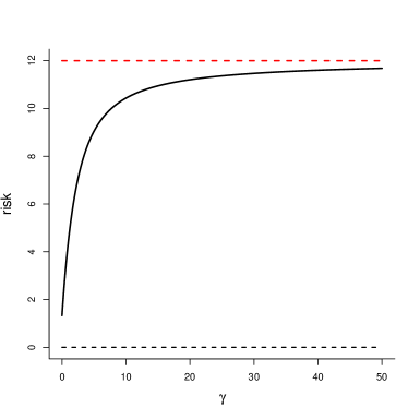
Figure 1: The risk functions of $\delta^{c}$ of (3.5) (full curve) and of $\delta_{0}=Y$ (constant, slanted), with $p=9$ and $c=3$.

3.3   Loss function robustness.

Robustness of performance statements with respect to the specific loss function used is often overlooked in the literature, as if the loss function worked with had been handed down from above with absolute precision. The matter is clearly of importance, however, as e.g. briefly pointed to in comments by both Berger (1983) and Morris (1983). If an estimator performs well with respect to one loss function ${\rm Lo}_{a}$, but not for another loss function ${\rm Lo}_{b}$, say, even when these two are close, it is a cause for concern. We argue here, however, that our estimator (3.5), derived under loss function $L_{c}$ of (1.3), is somewhat robust regarding the precise value of $c$.

First consider the estimator $\delta_{\text{CZ}}$ of (1.2), which uses $\phi_{0}(z)=(p-1)/\{p-1+z\}$. It satisfies the second requirement of Theorem 2, i.e. $\phi_{0}(z)z<\phi_{0}(z+1)(z+1)$ for all $z$, but it does not necessarily satisfy the first requirement, namely $0<\phi(z)\leq 2(p-1)/\{p-1+(1+c)z\}$ for all $z$. It is easy to verify that if $0\leq c\leq 1$ then it does satisfy this requirement, however, showing that $\delta_{\text{CZ}}$ has certain robustness properties with respect to the $L_{c}$ loss function: It is minimax and uniformly dominates $\delta_{0}$ under $L_{c}$, provided $0\leq c\leq 1$.

One can similarly study how the $\delta^{c_{0}}(Y)=[(1+c_{0})Z/\{p-1+(1+c_{0})Z\}]\,Y$ of (3.5) fares when the loss function is not quite the $L_{c_{0}}$ under which it was derived, but rather $L_{c}$, with another penalty value of $c$, that is, with a somewhat different penalty paid to incorrect estimation of the sum $\gamma$. From the first condition of Theorem 2 we see that $\delta^{c_{0}}$ is still minimax and uniformly better than $\delta_{0}=y$ under $L_{c}$, provided that $0\leq c\leq 2c_{0}+1$. An immediate implication of this is that all estimators in the class $\mathcal{D}_{c}$ are minimax and uniformly better than $\delta_{0}$ under the $L_{1}^{*}$ loss function, showing that the more prudent estimation strategy $\delta^{c}$, in the sense that it shrinks less that $\delta_{\text{CZ}}$, is robust to $c=0$.

4   Bayes, empirical Bayes, and admissibility

In this section a certain class of priors is studied along with Bayes and empirical Bayes consequences. The estimator $\delta^{c}$ of (3.5) will be shown to be both a natural generalised Bayes estimator with respect to a certain noninformative prior, and a natural empirical Bayes estimator with respect to independent Gamma priors. In addition, a class of proper Bayes estimators belonging to the class $\mathcal{D}_{c}$ is derived from another prior construction. Finally, we are also able to show that for each given $c$, the $\delta^{c}$ of (3.5) is an admissible estimator, under the $L_{c}$ loss function. In particular, the Clevenson–Zidek estimator (1.2) is admissible under the $L_{0}$ function for which it was derived. Our result hence generalises that of Johnstone (1984, Theorem 4.1).

4.1   Priors with sum independent of proportions.

In the following we model the means $(\theta_{1},\ldots,\theta_{p})$ in terms of the sum $\gamma=\sum_{i=1}^{p}\theta_{i}$ and proportions $\pi_{i}=\theta_{i}/\gamma$ for $i=1,\ldots,p$.

Lemma 1.

Suppose that $\gamma$ and $\pi=(\pi_{1},\ldots,\pi_{p})$ are independent with simultaneous prior density $q(\gamma)r(\pi_{1},\ldots,\pi_{p-1})$. This corresponds to a density

$$q\Bigl{(}\sum_{i=1}^{p}\theta_{i}\Bigr{)}\frac{1}{(\sum_{i=1}^{p}\theta_{i})^{p-1}}\,r\left(\frac{\theta_{1}}{\sum_{i=1}^{p}\theta_{i}},\ldots,\frac{\theta_{p-1}}{\sum_{i=1}^{p}\theta_{i}}\right)$$

for $(\theta_{1},\ldots,\theta_{p})$. The posterior distribution for $\theta$ given the data is on the same form: $\gamma$ and $(\pi_{1},\ldots,\pi_{p})$ are still independent, and

$$\begin{split}\gamma\,|\,y&\sim\text{const.}\,\gamma^{z}e^{-\gamma}q(\gamma),\\ \pi\,|\,y&\sim\text{const.}\,\pi_{1}^{y_{1}}\cdots\pi_{p-1}^{y_{p-1}}(1-\pi_{1}-\cdots-\pi_{p-1})^{y_{p}}r(\pi_{1},\ldots,\pi_{p-1}).\end{split}$$

Proof.

The first part in an exercise in the transformation of random variables, involving calculating the determinant of Jacobi matrix $|\partial(\gamma,\pi_{1},\ldots,\pi_{p-1})/\partial(\theta_{1},\ldots,\theta_{p})|=\big{(}\sum_{i=1}^{p}\theta_{i}\big{)}^{-(p-1)}$. The second part follows because the combined Poisson likelihood $\prod_{i=1}^{p}\theta_{i}^{y_{i}}e^{-\theta_{i}}/y_{i}!$ is proportional to $\gamma^{z}e^{-\gamma}\pi_{1}^{y_{1}}\cdots\pi_{p-1}^{y_{p-1}}(1-\pi_{1}-\cdots-\pi_{p-1})^{y_{p}}$. ∎

If in particular $(\pi_{1},\ldots,\pi_{p})$ has a Dirichlet prior distribution with parameters $(\alpha_{1},\ldots,\alpha_{p})$, then the posterior is another Dirichlet with updated parameters $(\alpha_{1}+y_{1},\ldots,\alpha_{p}+y_{p})$, and this holds regardless of the prior used for $\gamma$. The important case of independent $\theta_{i}$ from a Gamma $(\alpha,\beta)$ corresponds to a Gamma prior $(p\alpha,\beta)$ for $\gamma$ and an independent Dirichlet $(\alpha,\ldots,\alpha)$ for the proportions.

Suppose $(\pi_{1},\ldots,\pi_{p})$ comes from a symmetric Dirichlet $(\alpha,\ldots,\alpha)$ independent of $\gamma$, the latter coming from a suitable prior $q(\cdot)$. The Bayes estimator under the $L_{c}$ loss function takes the form (3.1), i.e. $\delta_{i}=\{(1+c)/(1+ca/b)\}a_{i}$, with

$$a_{i}=\big{\{}{\rm E}\,(\gamma^{-1}\pi_{i}^{-1}\,|\,y)\big{\}}^{-1}=\big{\{}{\rm E}\,(\gamma^{-1}\,|\,y)\big{\}}^{-1}\big{\{}{\rm E}\,(\pi_{i}^{-1}\,|\,y)\big{\}}^{-1}=\frac{K(z)}{K(z-1)}\frac{\alpha+y_{i}-1}{p\alpha+z-1},$$

and $b=\big{\{}{\rm E}\,(\gamma^{-1}\,|\,Y)\big{\}}^{-1}=K(z)/K(z-1)$, writing $K(z)=\int_{0}^{\infty}\gamma^{z}e^{-\gamma}q(\gamma)\,{\rm d}\gamma$. Letting in particular $\pi$ be uniform over the simplex we obtain the estimator

$$\begin{split}\delta_{B,i}(y)&=\frac{1+c}{1+ca/b}\,a_{i}=\frac{K(z)}{K(z-1)}\frac{1+c}{p-1+(1+c)z}y_{i}.\end{split}$$ (4.1)

We are now in a position to give three pleasing interpretations of the estimator $\delta^{c}$ of (3.5).

First, it is a generalised Bayes estimator. For if $\gamma$ is given a flat prior $q(\gamma)=1$ on the halfline, then $K(z)=\Gamma(z+1)$, which inserted in (4.1) gives $\delta_{B}=\delta^{c}$.

Second, it is a limit of Bayes estimators. Let the proportions $(\pi_{1},\ldots,\pi_{p})$ have a flat Dirichlet $(1,\ldots,1)$ prior, with an independent $\gamma$ from a Gamma $(1,\beta)$. The Bayes solution is then

$$\delta_{i}^{B}=\bigg{(}1-\frac{p-1}{p-1+(1+c)z}\bigg{)}\frac{y_{i}}{1+\beta},$$

and the limit as $\beta\to 0$ is again $\delta_{i}^{c}$ of (3.5).

Thirdly, it is a natural empirical Bayes estimator. To see one of several such constructions let the $\theta_{i}$ be independent ${\rm Gamma}(1,\beta)$. The corresponding exact Bayes solution is given in (3.3). Now $\beta$ is to be estimated from the data. The marginal distribution of $Z$ is found from the facts that $Z$ given $\gamma$ is Poisson with mean $\gamma$, and $\gamma$ is Gamma distributed with parameters $(p,\beta)$, so

$$\text{Pr}\{Z=z\}=\frac{\beta^{p}}{\Gamma(p)}\frac{1}{z!}\frac{\Gamma(p+z)}{(1+\beta)^{p+z}},\;\;z=0,1,2,\ldots.$$

The sum $Z$ is sufficient for $\beta$ and $Z/(p-1+Z)$ is found to be an unbiased estimator for $1/(1+\beta)$, for any $p\geq 2$. Inserting this data-based value in (3.3) produces once again $\delta^{c}$.

Finally, the Gamma $(1,\beta)$ prior construction may be extended to an hierarchical setup where a prior is put on the hyperparameter $\beta$. This extends the approach of Ghosh & Parsian (1981) from the $L_{1}^{*}$ of (1.1) to the $L_{c}$ setting. Let the parameter $\beta$ be distributed according to

$$s(\beta)\propto\beta^{\eta-1}(\beta+1)^{-(\eta+\zeta)}.$$ (4.2)

Utilising that

$${\rm E}\,\Bigl{(}{1\over\theta_{i}}\,|\,y\Big{)}={\rm E}\,{\rm E}\,\Bigl{(}{1\over\theta_{i}}\,|\,y,\beta\Bigr{)}={\rm E}\,\Bigl{(}{1+\beta\over y_{i}}\,|\,y\Bigr{)},$$

the Bayes solution is then

$$\delta_{i}^{B}(y)=\frac{(1+c)(p-1+z)}{p-1+(1+c)z}\frac{y_{i}}{{\rm E}\,(1+\beta\mid z)},$$ (4.3)

since $Z$ is sufficient for $\beta$. Also, $\beta$ given $Z=z$ is distributed as

$$\beta\,|\,z\sim\{B(\eta+p,\zeta+z)\}^{-1}\beta^{\eta+p-1}(1+\beta)^{-(\eta+\zeta+z+p)},$$

where $B(a,b)=\Gamma(a)\Gamma(b)/\Gamma(a+b)$ is the Beta function. Provided $\beta$ comes from the $s(\beta)$ of (4.2), and $0<\eta\leq(p-2-c)/(1+c)$, then the Bayes solution in (4.3), by virtue of belonging to the class $\mathcal{D}_{c}$, is minimax and uniformly dominates $\delta_{0}$. To see this, insert

$${\rm E}\,(1+\beta\,|\,z)=\frac{p+\eta+\zeta+z-1}{z+\zeta-1}$$

in (4.3), yielding

$$\delta_{i}^{B}(y)=\frac{(1+c)(p-1+z)}{p-1+(1+c)z}\frac{z+\zeta-1}{p+\eta+\zeta+z-1}y_{i}.$$ (4.4)

By some algebra we obtain that for the Bayes solution we here consider

$$\begin{split}\psi(z)&=p-1+(1+c)z-(1+c)(p-1+z)\frac{z+\zeta-1}{p+\eta+\zeta+z-1}\\ &=(1+c)\frac{(p-1+z)(p+\eta)}{p-1+\eta+\zeta+z}-c(p-1).\end{split}$$

This function is non-decreasing for all $z\geq 0$. Moreover, we see that it is bounded above by

$$\sup_{z\geq 0}\psi(z)=(1+c)(p+\eta)\leq 2(p-1),$$

since $\eta\leq(p-2-c)/(1+c)$. This means that the class of Bayes solutions in (4.4), with $\eta$ obeying the constraint mentioned, satisfy both conditions of Theorem 2.

4.2   Admissibility.

So far we have studied estimators that dominate the maximum likelihood estimator under the $L_{c}$ loss function. In this section we will prove that the estimator $\delta^{c}$ of (3.5) cannot be uniformly improved upon, that is, $\delta^{c}$ is admissible. The basic ingredient in this proof is the characterisation of admissibility given by Brown & Farrel (1988, Theorem 2.6). According to this theorem an estimator $\delta$ is admissible for $\theta$ under $(\delta-\theta)^{2}/\theta$ if and only if there exists a sequence of finite measures $\nu_{n}$ such that the Bayes solution with respect to $\nu_{n}$, say $\delta_{n}$, converges to $\delta$ as $n\to\infty$, and

$$\lim_{n\to\infty}\{\text{BR}(\delta,\nu_{n})-\text{MBR}(\nu_{n})\}=0.$$

This prior sequence has to satisfy certain conditions, the details of which are stated in Brown & Farrel (1988) and Johnstone (1984, pages 237-238). For our purpose, it is sufficient to know that such a sequence exists if $\delta$ is admissible.

Consider the class of estimators given by

$$\delta_{i}=\frac{(1+c)\kappa(Z)}{p-1+(1+c)Z}\,Y_{i}=\frac{(1+c)Y_{i}}{p-1+(1+c)Z}\,\kappa(Z)\quad{\rm for\ }i=1,\ldots,p.$$ (4.5)

The Bayes estimators of (4.1) are on this form with $\kappa(z)=K(z)/K(z-1)$; in particular the estimator $\delta^{c}$ of (3.5) is on this form, with $\kappa(z)=z$. As in Johnstone (1984), it turns out that estimators of the class (4.5) are admissible provided that $\kappa(Z)$ is admissible for $\gamma$ under the loss function $(\kappa-\gamma)^{2}/\gamma$. The theorem below is in part a restatement of his Theorem 4.1.

Theorem 3.

Estimators of the form (4.5) are admissible for $(\theta_{1},\ldots,\theta_{p})$ under $L_{c}$ if and only if $\kappa(Z)$ is admissible for $\gamma$ under $L(\gamma,\delta)=(\delta-\gamma)^{2}/\gamma$.

Proof.

The risk function of (4.5) under $L_{c}$ can be written

$$R_{c}(\delta,\theta)={\rm E}_{\gamma}\Bigl{\{}\frac{(1+c)^{2}Z}{p-1+(1+c)Z}L(\gamma,\kappa(Z))+\frac{(p-1)(1+c)\gamma}{p-1+(1+c)Z}\Bigr{\}},$$ (4.6)

with $L(\gamma,\delta)=(\kappa-\gamma)^{2}/\gamma$; see Appendix A for the derivation of this claim. Introduce $u(z)=(1+c)^{2}z/\{p-1+(1+c)z\}$ and write $\bar{L}(\delta,\gamma,z)=u(z)L(\gamma,\delta)$. Let $\delta$ and $\delta^{\prime}$ be of the form (4.5) with $\kappa(Z)$ and $\kappa^{\prime}(Z)$ respectively. If ${\rm E}_{\gamma}\big{\{}\bar{L}(\kappa^{\prime}(Z),\gamma,Z)\big{\}}-{\rm E}_{\gamma}\big{\{}\bar{L}(\kappa(Z),\gamma,Z)\big{\}}\leq 0$, with strict inequality for some $\gamma$, then $R_{c}(\delta,\theta)-R_{c}(\delta^{\prime},\theta)\leq 0$ with strict inequality for some $\theta$. This shows that if $\kappa(Z)$ is inadmissible under $L^{*}$, then $\delta$ is inadmissible under $L_{c}$.

The contrapositive statement is more enlightening: If $\delta$ is admissible under $L_{c}$ then $\kappa(z)$ is admissible under $\bar{L}$. Conversely, assume that $\kappa(Z)$ is admissible for $\gamma$ under $L$, let $\{\nu_{n}({\rm d}\gamma)\}_{n\geq 1}$ be a sequence of prior measures satisfying the conditions of Brown & Farrel (1988, Theorem 2.6), and let $\rho_{n}(A)=\Gamma(p)\int_{A}\nu_{n}({\rm d}\gamma)\prod_{i=1}^{p}{\rm d}\pi_{i}$ be the prior measure over $(0,\infty)\times S$, where $S$ is the $(p-1)$-dimensional simplex. Then, since $0<u(z)<1+c$ for all $z\geq 1$,

$$\text{BR}_{c}(\delta,\rho_{n})-\text{BR}_{c}(\delta_{n},\rho_{n})\leq(1+c)\int{\rm E}_{\gamma}\{L(\gamma,\kappa(Z))-L(\gamma,\kappa_{n}(Z))\}\,{\rm d}\nu_{n}(\gamma).$$

The right hand side is non-negative for all $n$ since $\delta_{n}$ is the Bayes solution, and it also tends to zero by Theorem 2.6 in Brown & Farrel (1988) because $\kappa(z)$ is admissible. This implies admissibility of $\delta$ under $L_{c}$. ∎

The immediate corollary to Theorem 3 is that the estimator $\delta^{c}$ of (3.5) is admissible under $L_{c}$, because $\kappa(Z)=Z$ is admissible under the weighted squared error loss function $L(\gamma,\delta)=(\delta-\gamma)^{2}/\gamma$. As a special case, the Clevenson–Zidek estimator (1.2) is admissible under the $\sum_{i=1}^{p}(\delta_{i}-\theta_{i})^{2}/\theta_{i}$ loss function.

5   Smoothing towards the mean

In the following we consider different strategies for smoothing the maximum likelihood estimator towards the mean of the observations. Pushing the maximum likelihood estimator towards a data-based point should in many cases yield more reduction in risk than pushing $\delta_{0}$ towards the origin, particularly when the $\theta_{i}$ are not small and not too spread out. This is clearly visible in Figure 1 where the improvement in risk of $\delta^{c}$ compared to $\delta_{0}$ becomes smaller as $\gamma=\sum_{i=1}^{p}\theta_{i}$ grows; the improvement in risk is, in other words, biggest near the ‘point of attraction’.

Ghosh, Hwang & Tsui (1983) considered a modification of $\delta_{\text{CZ}}$ that shrinks the maximum likelihood estimator towards the minimum of the observations, and were able to prove uniform dominance under the weighted loss $L_{1}^{*}$ of (1.1), for their modified estimator. Albert (1981) took the Bayes estimator under $L_{0}(\theta,\delta)=\sum_{i=1}^{p}(\delta_{i}-\theta_{i})^{2}$ as his point of departure, and developed an estimator that pushes the observations towards the mean $\bar{y}$ and performs better than the usual estimator in large parts of the parameter space.

A complication when working with the $L_{c}$ loss function of (1.4) is that we compete with the maximum likelihood estimator on two turfs, so to speak, namely under $\sum_{i=1}^{p}(\delta_{i}-\theta_{i})^{2}/\theta_{i}$ and under $\big{(}\sum_{i=1}^{p}\delta_{i}-\gamma\big{)}^{2}/\gamma$. One reason for choosing the mean as our ‘point of attraction’ is that several of the estimators we construct preserve the mean, that is, $\sum_{i=1}^{p}\delta_{i}(Y)=Z$. In this way such new estimators will always ‘match’ the risk performance of $\delta_{0}$ when it comes estimating $\gamma$, and the penalty parameter $c$ becomes immaterial.

5.1   A restricted minimax estimator.

Consider estimators of the form

$$\delta_{i}(Y)=Y_{i}-g(Z)(Y_{i}-\bar{Y}),$$ (5.1)

where $\bar{Y}=Z/p$. Notice that $\sum_{i=1}^{p}\delta_{i}=Z=\sum_{i=1}^{p}\delta_{0,i}$, which means that in calculations of the difference in risk between estimators of the form (5.1) and $\delta_{0}=Y$, the $c$-term in the $L_{c}$ loss function disappears. The value of $g(0)$ is immaterial, since $\delta$ is then equal to zero, and we may take $g(0)=0$ for convenience.

Using that $Y$ given $Z=z$ is multinomial with cell probabilities $\pi_{i}$, for each $z\geq 1$, the risk difference $R_{c}(\delta,\theta)-R_{c}(\delta_{0},\theta)$ can be expressed as

$$d(\theta) = {\rm E}_{\theta}\sum_{i=1}^{p}\frac{1}{\theta_{i}}\left\{g(Z)^{2}(Y_{i}-Z/p)^{2}-2g(Z)(Y_{i}-Z/p)(Y_{i}-\theta_{i})\right\}$$

$$= {\rm E}_{\theta}\sum_{i=1}^{p}\left[g(Z)^{2}\left\{Z\frac{1-\pi_{i}}{\gamma}+\pi_{i}\frac{Z^{2}}{\gamma}-2\frac{Z^{2}}{p\gamma}+\frac{Z^{2}}{p^{2}\theta_{i}}\right\}\right.$$

$$\hskip 56.9055pt\left.-2g(Z)\left\{Z\frac{1-\pi_{i}}{\gamma}+\pi_{i}\frac{Z^{2}}{\gamma}-Z\pi_{i}-\frac{Z^{2}}{p\gamma}+\frac{Z}{p}\right\}\right]$$

$$= {\rm E}_{\theta}\left[g(Z)^{2}\left\{Z\frac{p-1-Z}{\gamma}+\frac{Z^{2}}{p^{2}\gamma}\sum_{i=1}^{p}\pi_{i}^{-1}\right\}-2g(Z)Z\frac{p-1}{\gamma}\right]$$

$$= {\rm E}_{\theta}\left[g(Z)^{2}\left\{Z\frac{p-1-Z}{\gamma}+\frac{Z^{2}}{p\gamma}B(\pi)\right\}-2g(Z)Z\frac{p-1}{\gamma}\right]$$

$$= {\rm E}_{\theta}\Bigl{(}g(Z+1)^{2}\left[p-1+(Z+1)\{B(\pi)/p-1\}\right]-2(p-1)g(Z+1)\Bigr{)},$$

writing

$$B(\pi)=p^{-1}\sum_{i=1}^{p}\pi_{i}^{-1}$$ (5.2)

for the mean of the inverse proportions. It is not possible to find a function $g(\cdot)$ such that the estimator in (5.1) dominates $\delta_{0}=Y$ over the entire parameter space $\Theta=(0,\infty)^{p}$. This is the ‘tyranny of the boundary’ phenomenon; as a single $\theta_{i}\to 0$ the sum $B(\pi)\to\infty$ and the risk blows up for non-null choices of $g$.

Estimators can be found, however, that dominate $\delta_{0}$ over large proportions of the parameter space. Let $\Theta(b_{0})\subset\Theta$ be the subset of the parameter space where $B(\pi)\leq pb_{0}$. The minimum value of $B(\pi)$ is $p$, so $b_{0}>1$. In some situations one might have prior grounds for believing that the $\theta_{i}$ are somewhat similar, that is, not too far from the mean $\bar{\theta}$. One might for example have that each $\theta_{i}\geq\varepsilon\bar{\theta}=\varepsilon\gamma/p$, or equivalently $\pi_{i}\geq\varepsilon/p$, for some small $\varepsilon>0$. This implies that $B(\pi)\leq p/\varepsilon$, so $b_{0}=1/\varepsilon$ may be used, so the risk difference can be bounded:

$$d(\theta)\leq{\rm E}_{\theta}\,g(Z+1)\left\{g(Z+1)[p-1+(Z+1)(b_{0}-1)]-2(p-1)\right\}.$$ (5.3)

Based on this upper bound we derive the estimator with

$$\delta^{*}_{i}(Y)=Y_{i}-\frac{p-1}{p-1+(b_{0}-1)Z}(Y_{i}-\bar{Y})\quad{\rm for\ }i=1,\ldots,p.$$ (5.4)

This estimator succeeds in having

$$R_{c}(\delta^{*},\theta) \leq R_{c}(\delta_{0},\theta)-{\rm E}_{\theta}\frac{(p-1)^{2}}{p-1+(b_{0}-1)(Z+1)}$$

$$< p+c-(p-1)^{2}/\{p-1+(b_{0}-1)(\gamma+1)\}$$

for all $\theta\in\Theta(b_{0})$, with the last inequality following from Jensen’s.

5.2   A restricted Bayes estimator.

The estimator in (5.4) was derived with the aim of risk function dominance in a given large region $\Theta(b_{0})$ of the parameter space. We may also derive the restricted Bayes solution, that is, the best estimator among those of the form (5.1), under a prior of the type discussed in Section 4. Since $\gamma$ and $\pi$ are independent, the Bayes risk of such an estimator is

$$\text{BR}_{c}(\delta) = p+c-{\rm E}^{q}\,{\rm E}_{\gamma}\big{\{}2(p-1)g(Z+1)$$

$$\qquad-g(Z+1)^{2}[p-1+\{{\rm E}^{r}\,B(\pi)/p-1\}(Z+1)]\big{\}},$$

where ${\rm E}^{q}\,(\cdot)$ and ${\rm E}^{r}\,(\cdot)$ are the expectations of $\gamma$ and $\pi$ with respect to their prior distributions, cf. Lemma 1. If we now let ${\rm E}^{r}\,B(\pi)=pb_{0}$, this reproduces the estimator in (5.4), but with a differently interpreted $b_{0}$. The risk function is

$$R_{c}(\delta^{B},\theta)=p+c-(p-1)\,{\rm E}_{\gamma}\,g(Z+1)\Bigl{[}2-\frac{p-1+\{B(\pi)/p-1\}(Z+1)}{p-1+(b_{0}-1)(Z+1)}\Bigr{]},$$

with $g(z)=(p-1)/\{p-1+(b_{0}-1)z\}$. Consider again the prior construction of Section 4. If $(\pi_{1},\ldots,\pi_{p})$ comes from a Dirichlet distribution with parameters $(\alpha,\ldots,\alpha)$, then $b_{0}=(\alpha-1/p)/(\alpha-1)$, provided that $\alpha>1$. Recall that the inequality in 5.3 only holds if $b_{0}>1$, which means that the subspace $\Theta(b_{0})$ is empty if our prior knowledge dictates $0<\alpha\leq 1$. On the other side of the spectrum, as $\alpha\to\infty$ this estimator would assign the estimate $1/p$ to each of the proportions, and since $b_{0}$ goes to one as $\alpha$ goes to infinity, the estimator (5.4) tends to $\bar{y}=z/p$. In other words, having smaller values of $\alpha>1$ expands the space $\Theta(b_{0})$ but results in less gain in risk.

The (5.4) estimator may also use a data-based value for $b_{0}$. With $\pi$ and $\gamma$ independent, the marginal distribution of the data is

$$\int_{S}\int_{0}^{\infty}f(y\,|\,\pi,\gamma)r(\pi)q(\gamma)\,{\rm d}\gamma\,{\rm d}\pi_{1}\cdots{\rm d}\pi_{p-1}\propto\frac{\Gamma(p\alpha)}{\Gamma(\alpha)^{p}}\frac{\prod_{i=1}^{p}\Gamma(\alpha+y_{i})}{\Gamma(p\alpha+z)}.$$

This likelihood can be maximised to obtain an estimate $\widehat{\alpha}$ which is plugged into $b_{0}=(\alpha-1/p)/(\alpha-1)$, again provided that $\widehat{\alpha}>1$.

5.3   More careful smoothing towards the mean.

We now consider the construction

$$\widehat{\theta}_{i}=Y_{i}-g(Z)(Y_{i}-\bar{Y})h(Y),$$

where $h(y)$ is a function such that if one or more $y_{i}=0$, then $h(y)=h(y_{1},\ldots,y_{p})=0$. The intention is that of more careful smoothing towards the mean than with (5.1), to achieve risk improvement in potentially larger parts of the parameter space. Note that $\sum_{i=1}^{p}\widehat{\theta}_{i}=\sum_{i=1}^{p}y_{i}$, so any risk difference $R_{c}(\widehat{\theta},\theta)-R_{c}(Y,\theta)$ does not depend on the $c$ term of the loss function. Also, the value of $g(z)$ at $z=0$ is immaterial, so we may take $g(0)=0$, for convenience.

To work with the risk functions, we start from

$$(\widehat{\theta}_{i}-\theta_{i})^{2}-(y_{i}-\theta_{i})^{2}=g(z)^{2}(y_{i}-\bar{y})^{2}h(y)^{2}-2g(z)(y_{i}-\bar{y})h(y)(y_{i}-\theta_{i}).$$

The risk difference $R_{c}(\widehat{\theta},\theta)-R_{c}(Y,\theta)$ may hence be expressed as

$${\rm E}_{\theta}\sum_{i=1}^{p}\{{g(Z)^{2}(Y_{i}-\bar{Y})^{2}h(Y)^{2}-2g(Z)(Y_{i}-\bar{Y})h(Y)(Y_{i}-\theta_{i})}\}/\theta_{i}={\rm E}_{\theta}\,D(Y),$$

with

$$D(y) = \sum_{i=1}^{p}\Bigl{[}{g(z+1)^{2}\{y_{i}+1-(z+1)/p)\}^{2}h(y+e_{i})^{2}\over y_{i}+1}$$

$$\qquad-2g(z+1)\{y_{i}+1-(z+1)/p\}h(y+e_{i})+2g(z)(y_{i}-\bar{y})h(y)\Bigr{]}$$

$$= g(z+1)^{2}\Bigl{\{}\sum_{i=1}^{p}(y_{i}+1)h(y+e_{i})^{2}$$

$$\qquad-2{z+1\over p}\sum_{i=1}^{p}h(y+e_{i})^{2}+{(z+1)^{2}\over p^{2}}\sum_{i=1}^{p}{h(y+e_{i})^{2}\over y_{i}+1}\Bigr{\}}$$

$$\qquad-2g(z+1)\Bigl{\{}\sum_{i=1}^{p}(y_{i}+1)h(y+e_{i})-{z+1\over p}\sum_{i=1}^{p}h(y+e_{i})\Bigr{\}}.$$

The property that $y_{i}=0$ implies $h(y)=0$ is actively used here; without such a constraint, more complicated terms need to be added to the ${\rm E}_{\theta}\,D(Y)$ here.

Several choices may be considered and worked with for further fine-tuning, regarding the $h(y)$ function. For the present report we limit attention to the special case of $h_{0}(y)=I\{{\rm each\ }y_{i}\geq 1\}$. We need to study and bound the $D(y)$ function with this choice of $h(y)$. Note that $\sum_{i=1}^{p}h_{0}(y+e_{i})$ is $p$, if all $y_{i}\geq 1$; is 1, if one and only one of $y_{i}=0$; and is 0, otherwise. Similarly, $\sum_{i=1}^{p}y_{i}h_{0}(y+e_{i})=z$, if all $y_{i}\geq 1$; and 0, otherwise. Furthermore,

$$\sum_{i=1}^{p}{h_{0}(y+e_{i})\over y_{i}+1}\begin{cases}\leq p/2&\quad{\rm if\ all\ }y_{i}\geq 1,\\ =1&\quad{\rm if\ only\ one\ }y_{i}=0,\\ =0&\quad{\rm otherwise}.\end{cases}$$

(i) Assume first that all $y_{i}\geq 1$. Then

$$D(y) = g(z+1)^{2}\Bigl{\{}z+p-2(z+1)+{(z+1)^{2}\over p^{2}}\sum_{i=1}^{p}{1\over y_{i}+1}\Bigr{\}}-2g(z+1)(p-1)$$

$$\leq g(z+1)^{2}\Bigl{\{}p-1-(z+1)+\hbox{$1\over 2$}{(z+1)^{2}\over p}\Bigr{\}}-2g(z+1)(p-1).$$

The function $p-1-x+\hbox{$1\over 2$}x^{2}/p$ for $x\geq 1$ has its minimum value at position $x=p$, with minimum value $\hbox{$1\over 2$}p-1$, which is positive as long as $p\geq 3$. (ii) When there is only one $y_{i}=0$, the rest $y_{j}\geq 1$, we find

$$D(y) = g(z+1)^{2}\Bigl{\{}0+1-2{z+1\over p}1+{(z+1)^{2}\over p^{2}}1\Bigr{\}}-2g(z+1)\Bigl{\{}0+1-{z+1\over p}0\Bigr{\}}$$

$$= g(z+1)^{2}\Bigl{\{}-2{z+1\over p}+{(z+1)^{2}\over p^{2}}\Bigr{\}}-2g(z+1).$$

(iii) Otherwise, which means that the number of $y_{i}=0$ is between 2 and $p-1$, we find that $D(y)=0$.

Our best choice for $g(z)$, based on the upper risk bound for the case of all $y_{i}\geq 1$, is

$$g_{0}(z+1)={p-1\over p-1-(z+1)+\hbox{$1\over 2$}(z+1)^{2}/p},\quad{\rm or}\quad g_{0}(z)={p-1\over p-1-z+\hbox{$1\over 2$}z^{2}/p}.$$

The estimator

$$\begin{array}[]{rcl}\widehat{\theta}_{i}&=&\displaystyle Y_{i}-g_{0}(Z)(Y_{i}-\bar{Y})h_{0}(Y)\\ &=&\displaystyle Y_{i}-{p-1\over p-1-Z+\hbox{$1\over 2$}Z^{2}/p}(Y_{i}-\bar{Y})I\{{\rm all\ }Y_{i}\geq 1\},\end{array}$$ (5.7)

therefore, has risk function $R_{c}(\widehat{\theta})=p+c+{\rm E}_{\theta}\,D_{0}(Y)$, where an exact expression for $D_{0}(Y)$ is found via the above. We also know that

$$D_{0}(y)\leq-{(p-1)^{2}\over p-1-(z+1)+\hbox{$1\over 2$}(z+1)^{2}/p}\quad{\rm if\ all\ }y_{i}\geq 1\,;$$

that

$$D_{0}(y) = \Bigl{\{}{p-1\over p-1-(z+1)+\hbox{$1\over 2$}(z+1)^{2}/p}\Bigr{\}}^{2}\Bigl{\{}-2{z+1\over p}+{(z+1)^{2}\over p^{2}}\Bigr{\}}$$

$$\qquad\qquad-2{p-1\over p-1-(z+1)+\hbox{$1\over 2$}(z+1)^{2}/p},$$

for the cases of $y$ where precisely one $y_{i}=0$, the other $y_{j}\geq 1$; and finally that $D_{0}(y)=0$ for those $y$ for which the number of $y_{i}=0$ is between 2 and $p-1$. As long as all $\theta_{i}$ are at least moderate, so that $h_{0}(Y)=1$ with high probability, there is clear risk improvement on the minimax risk $p+c$. The corner cases, however, where one $\theta_{i}$ is small and the others not, are the ‘bad cases’ for the (5.7) estimator, where the risk might become larger than $p+c$. Since $D_{0}(y)$ flattens to zero when $z=\sum_{i=1}^{p}y_{i}$ increases, the risk converges to $p+c$ for all $\theta=\gamma(\pi_{1},\ldots,\pi_{p})$ where $\gamma$ tends to infinity.

6   Bayes and empirical Bayes with more structure

In the previous sections we have constructed and analysed estimators essentially symmetric in the observations. Sometimes some structure is anticipated in the parameters, however, as with setting up regressions or log-linear models for Poisson tables, see e.g. Agresti (2019), or with classes of priors. The present section briefly complements our earlier efforts by examining risk function consequences for estimators that favour asymmetric structures.

6.1   Risk functions with Gamma priors.

A natural class of priors takes independent Gamma priors, with parameters $(\alpha_{i},\beta)$, for the $\theta_{i}$. As was seen in Section 3, the Bayes estimator then takes the form

$$\delta_{i}^{B}=h_{c}(z){\alpha_{i}+y_{i}-1\over\beta+1}\quad{\rm with}\quad h_{c}(z)={(1+c)(p\bar{\alpha}+z-1)\over(1+c)(p\bar{\alpha}+z-1)-c(p-1)},$$ (6.1)

writing $\bar{\alpha}$ for $(1/p)\sum_{i=1}^{p}\alpha_{i}$; also, for cases where $\alpha_{i}<1$ and $y_{i}=0$, the estimator is zero.

The present task is to study the consequent risk functions, for such estimators, outside the special and simplest case where each $\alpha_{i}=1$. The point will be that estimators then lose the minimax property, with the risk exceeding the $p+c$ benchmark level when one or more of the $\theta_{i}$ come close to zero, but that the risk otherwise can be lower than $p+c$ in big and reasonable parts of the parameter space. For simplicity of presentation we restrict attention here to the case of $c=0$. Similar results and insights may be reached for the general loss function $L_{c}$, using more laborious methods we develop and exploit for somewhat different purposes in Section 6.2. For the ensuing estimator $(\alpha_{i}+Y_{i}-1)/(\beta+1)$, some calculations yield

$$R(\delta^{B},\theta) = \sum_{i=1}^{p}{1\over\theta_{i}}\Bigl{[}\Bigl{\{}{\alpha_{i}+\theta_{i}-1-(\beta+1)\theta_{i}\over\beta+1}\Bigr{\}}^{2}+{\theta_{i}\over(\beta+1)^{2}}\Bigr{]}$$

$$= {1\over(\beta+1)^{2}}\Bigl{\{}\sum_{i=1}^{p}{(\alpha_{i}-1-\beta\theta_{i})^{2}\over\theta_{i}}+p\Bigr{\}}.$$

This is smaller than or equal to $R(Y,\theta)=p$ when

$$A(\theta)={1\over p}\sum_{i=1}^{p}{(\alpha_{i}-1-\beta\theta_{i})^{2}\over\beta\theta_{i}}\leq{(\beta+1)^{2}-1\over\beta}=2+\beta.$$

This defines a fairly large parameter region, $\{\theta\colon A(\theta)\leq 2+\beta\}$, with the $1/\theta_{i}$ not being too far away from the prior mean values $\beta/(\alpha_{i}-1)$, and where using the Bayes estimator hence is better than with the $\delta_{0}=Y$ method. Under the prior itself, the random $A(\theta)$ has mean

$${1\over p}\sum_{i=1}^{p}\Bigl{\{}{(\alpha_{i}-1)^{2}\over\beta}{\beta\over\alpha_{i}-1}-2(\alpha_{i}-1)+\beta{\alpha_{i}\over\beta}\Bigr{\}}=1,$$

and variance of order $O(1/p)$, showing that only rather unlikely values of $\theta$ will have risk above the benchmark $p$.

6.2   Risks for a class of empirical Bayes estimators.

With the independent Gamma priors used above we next note that the marginal distribution of $y_{i}$ becomes

$$g(y_{i}\,|\,\alpha_{i},\beta) = \int_{0}^{\infty}{\beta^{\alpha_{i}}\over\Gamma(\alpha_{i})}\theta_{i}^{\alpha_{i}-1}\exp(-\beta\theta_{i}){1\over y_{i}!}\exp(-\theta_{i})\theta_{i}^{y_{i}}\,{\rm d}\theta_{i}$$

$$= {\beta^{\alpha_{i}}\over\Gamma(\alpha_{i})}{1\over y_{i}!}{\Gamma(\alpha_{i}+y_{i})\over(\beta+1)^{\alpha_{i}+y_{i}}},$$

for $y_{i}=0,1,2,\ldots$. In the setup where the $\alpha_{i}$ are taken known but $\beta$ an unknown parameter, we see that $Z=\sum_{i=1}^{p}Y_{i}$ is sufficient. Since $Z$ given the parameters is Poisson with mean $\gamma=\sum_{i=1}^{p}\theta_{i}$, and $\gamma$ is Gamma $(p\bar{\alpha},\beta)$, writing $\bar{\alpha}=(1/p)\sum_{i=1}^{p}\alpha_{i}$, its distribution may be written

$$q(z\,|\,\beta)={\beta^{p\bar{\alpha}}\over\Gamma(p\bar{\alpha})}{1\over z!}{\Gamma(p\bar{\alpha}+z)\over(\beta+1)^{p\bar{\alpha}+z}}\quad{\rm for\ }z=0,1,2,\ldots.$$

From this we can derive

$${\rm E}\,{Z\over p\bar{\alpha}-1+Z}=\sum_{z=1}^{\infty}{1\over(z-1)!}{\beta^{p\bar{\alpha}}\over\Gamma(p\bar{\alpha})}{\Gamma(p\bar{\alpha}+z-1)\over(\beta+1)^{p\bar{\alpha}+z-1}}{1\over\beta+1}={1\over\beta+1},$$ (6.2)

provided only that $p\geq 2$. Hence $Z/(p\bar{\alpha}-1+Z)$ can be used as an estimator for the quantity $1/(\beta+1)$. With pre-specified $\alpha_{i}$, then, a natural empirical Bayes version of estimator (6.1) emerges:

$$\begin{array}[]{rcl}\widehat{\theta}_{i}&=&\displaystyle{(1+c)(p\bar{\alpha}-Z-1)\over(1+c)(p\bar{\alpha}+Z-1)-c(p-1)}{Z\over p\bar{\alpha}-1+z}(\alpha_{i}+Y_{i}-1)\\ &=&\displaystyle h_{c}(Z)(\alpha_{i}+Y_{i}-1),\end{array}$$ (6.5)

with

$$h_{c}(Z)={(1+c)Z\over(1+c)(p\bar{\alpha}+Z-1)-c(p-1)}.$$

In particular, under $L_{0}$ loss, with $c=0$, the natural empirical Bayes estimator is

$$\widehat{\theta}_{i}=h_{0}(Z)(\alpha_{i}+Y_{i}-1)={Z\over p\bar{\alpha}+Z-1}(\alpha_{i}+Y_{i}-1),$$ (6.6)

generalising the earlier symmetric case with all $\alpha_{i}=1$, which yields the already studied minimax and admissible estimator (1.5).

Expressions for the risk function $R_{c}(\widehat{\theta},\theta)$ can now be worked out, using the fact that $y_{i}\,|\,z$ is binomial $(z,\pi_{i})$, with $\pi_{i}=\theta_{i}/\gamma$. Consider the general class of estimators

$$\widehat{\theta}_{i}=h(Z)(\alpha_{i}+Y_{i}-1)\quad{\rm for\ }i=1,\ldots,p.$$ (6.7)

The $h(z)$ functions we are encountering all have $h(0)=0$, and will in fact have the form $q(z)z$, for suitable $q(z)$. Also, they will be nondecreasing with $h(z)\rightarrow 1$ as $z$ increases. The task now is to develop formulae for their risk functions, through suitable representations of the form

$$R(\widehat{\theta},\theta)={\rm E}_{\theta}\,H(Z,\theta)=\sum_{z=1}^{\infty}H(z,\theta)\exp(-\gamma)\gamma^{z}/z!,$$

and then showing, for relevant choices of $h(z)$, that this is less than $p+c$ for large and relevant parameter regions.

We start from

$${\rm E}_{\theta}\,{1\over\theta_{i}}\{h(z)(\alpha_{i}+Y_{i}-1)-\theta_{i}\}^{2}\,|\,z = {1\over\gamma\pi_{i}}[\{h(z)(\alpha_{i}+z\pi_{i}-1)-\gamma\pi_{i}\}^{2}$$

$$\qquad\qquad+\,h(z)^{2}z\pi_{i}(1-\pi_{i})]$$

$$= {1\over\gamma\pi_{i}}\bigl{\{}[h(z)(\alpha_{i}-1)+\{h(z)z-\gamma\}\pi_{i}]^{2}$$

$$\qquad\qquad+\,h(z)^{2}z\pi_{i}(1-\pi_{i})\bigr{\}}.$$

For the case of $c=0$ this leads to

$$H(z,\theta) = h(z)^{2}\sum_{i=1}^{p}{(\alpha_{i}-1)^{2}\over\gamma\pi_{i}}+\{h(z)z-\gamma\}^{2}{1\over\gamma}$$

$$\qquad\qquad+\,2\{h(z)z-\gamma\}h(z)(p\bar{\alpha}-p){1\over\gamma}+h(z)^{2}z(p-1){1\over\gamma}.$$

For the ‘$c$ term’ part of the risk, note that $\widehat{\theta}_{i}=h(z)(p\bar{\alpha}+z-p)$, leading to

$${\rm E}_{\gamma}\,{\{h(Z)(p\bar{\alpha}+Z-p)-\gamma\}^{2}\over\gamma}={\rm E}_{\gamma}\,{\{h(Z)Z-\gamma+h(Z)(p\bar{\alpha}-p)\}^{2}\over\gamma}.$$

This may be exploited further using the identity ${\rm E}_{\gamma}\,r(Z)/\gamma={\rm E}_{\gamma}\,r(Z+1)/(Z+1)$ for functions $r(z)$ with $r(0)=0$.

For brevity we limit attention here to the case of $c=0$; extensions can be worked out using the same methods. We use the identity pointed to for

$$\{h(z)z-\gamma\}^{2}/\gamma=h(z)^{2}z^{2}/\gamma-2h(z)z+\gamma,$$

and find $R(\widehat{\theta},\theta)={\rm E}_{\gamma}\,Q(Z,\theta)$, with

$$Q(z,\theta) = h(z)^{2}\sum_{i=1}^{p}{(\alpha_{i}-1)^{2}\over\gamma\pi_{i}}+h(z+1)^{2}(z+1)-2h(z)z+\gamma$$

$$\qquad+\,2{\{h(z+1)(z+1)-\gamma\}h(z+1)\over z+1}(p\bar{\alpha}-p)+h(z+1)^{2}(p-1).$$

The risk function may hence be expressed as

$$R(\widehat{\theta},\theta)=pm_{1}(\gamma)\,C(\pi)/\gamma+R_{1}(\gamma)+2(p\bar{\alpha}-p)R_{2}(\gamma)+(p-1)m_{2}(\gamma),$$ (6.8)

in which $C(\pi)=(1/p)\sum_{i=1}^{p}(\alpha_{i}-1)^{2}/\pi_{i}$, and

$$m_{1}(\gamma) = {\rm E}_{\gamma}\,h(Z)^{2},$$

$$m_{2}(\gamma) = {\rm E}_{\gamma}\,h(Z+1)^{2},$$

$$R_{1}(\gamma) = {\rm E}_{\gamma}\,\{h(Z+1)^{2}(Z+1)-2h(Z)Z+\gamma\},$$

$$R_{2}(\gamma) = {\rm E}_{\gamma}\,{\{h(Z+1)(Z+1)-\gamma\}h(Z+1)\over Z+1}.$$

Here $m_{1}(\gamma)$ and $m_{2}(\gamma)$ are inside $(0,1)$, and increase to 1; the $R_{1}(\gamma)$ and $R_{2}(\gamma)$ are bounded and converge to respectively one and zero as $\gamma$ increases. For larger $\gamma$, therefore, the risk goes to the minimax risk $p$. The risk function (6.8) may exceed the minimax threshold level $p$ if one or more of the $\pi_{i}=\theta_{i}/\gamma$ are small, but even for small $\pi_{i}$ the risk decreases with increasing $\gamma$. Otherwise the situation is that the risk may become significantly smaller than $p$ in parts of the parameter space not disagreeing much from what is judged likely under the prior, and that it can be smaller than $p$ also in other larger parameter regions. An upper bound is

$$R(\widehat{\theta},\theta)\leq pm_{1}(\gamma)\{\max_{i\leq p}|\alpha_{i}-1|\}^{2}B(\pi)/\gamma+R_{1}(\gamma)+2(p\bar{\alpha}-p)R_{2}(\gamma)+(p-1)m_{2}(\gamma),$$

with $B(\pi)$ as in (5.2). This may in particular be investigated further, with the choice $h_{0}(z)$, corresponding to the estimator (6.6). The risk function is bounded; converges to the minimax value $p$ when $\gamma$ increases, regardless of proportions $(\pi_{1},\ldots,\pi_{p})$; may offer substantial improvement for sizeable portions of the parameter space; and its maximum value is often not much bigger than $p$.

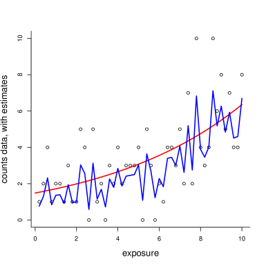
Figure 2: Estimating $p=50$ Poisson parameters, in a simulated regression setting with $(x_{i},y_{i})$ data, with the empirical Bayes method (6.6), shrinking the raw estimates $y_{i}$ towards prior means $\alpha_{i}/\beta$, with $\beta$ estimated from the data.

An illustration of the empirical Bayes strategy (6.6) is provided in Figure 2, in a situation with simulated regression data $(x_{i},y_{i})$. The prior takes the $\theta_{i}$ to stem from Gamma $(\alpha_{i},\beta)$, with $\alpha_{i}=\exp(\gamma_{0}+\gamma_{1}x_{i})$, for suitable prior guess values $(\gamma_{0},\gamma_{1})$, and then estimates $\beta$ from data, as per (6.2). Similar Bayes and empirical Bayes methods can be developed for priors of the type $\theta_{i}\sim{\rm Gamma}(d\theta_{0,i},d)$, with either hyperpriors on the prior parameters $\theta_{0,i}$ and $d$, or involving estimators for these from the data.

7   Estimation with a weighted loss function

Above we have worked with our loss function $L_{c}$, a natural extension of the Clevenson–Zidek loss function $L_{1}^{*}(\theta,\delta)=\sum_{i=1}^{p}(\delta_{i}-\theta_{i})^{2}/\theta_{i}$, to account for not shrinking the mean too much. Another useful extension is to allow for weighting, with

$$L_{w}(\theta,\delta)=\sum_{i=1}^{p}w_{i}(\delta_{i}-\theta_{i})^{2}/\theta_{i},$$

where $w_{1},\ldots,w_{p}$ are fixed, positive, and context driven, reflecting relative importance. This is e.g. important when the $y_{i}$ result from different levels of exposure, as with $y_{i}$ stemming from a Poisson with parameter $w_{i}\theta_{i}$. The $\delta_{0}=Y$ estimator is again the natural benchmark; it has constant risk $w_{0}=\sum_{i=1}^{p}w_{i}$, and it is minimax. To prove this second claim, one may work with the prior where the $\theta_{i}$ are independent and Gamma distributed, with parameters $(\alpha,\beta)$, and with $\alpha\geq 1$ to avoid a certain technical issue. Some work shows that the Bayes estimator becomes $\widehat{\theta}_{i}=1/{\rm E}\,(\theta_{i}\,|\,y)=(\alpha+y_{i}-1)/(\beta+1)$, with associated minimum Bayes risk as simple as $w_{0}/(\beta+1)$. Letting $\beta\rightarrow 0$ we have convergence to the constant risk of $\delta_{0}$.

This estimator may be uniformly improved upon, however, as we now demonstrate, yielding another generalisation of the Clevenson–Zidek estimator. Consider estimators of the form

$$\widehat{\theta}_{i}=\{1-\phi(V)\}Y_{i}\quad{\rm for\ }i=1,\ldots,p,\quad{\rm where\ }V=v(Y)=\sum_{i=1}^{p}w_{i}Y_{i}.$$ (7.1)

Using the identity (3.4) we may express the risk difference $r_{w}$ between $\widehat{\theta}$ and $\delta_{0}$, i.e. ${\rm E}_{\theta}\,\{L_{w}(\theta,\widehat{\theta})-L_{w}(\theta,\delta_{0})\}$, as

$$r_{w} = {\rm E}_{\theta}\sum_{i=1}^{p}{w_{i}\over\theta_{i}}\{\phi(V)^{2}Y_{i}^{2}-2\phi(V)Y_{i}(Y_{i}-\theta_{i})\}$$

$$= {\rm E}_{\theta}\sum_{i=1}^{p}w_{i}\bigl{[}\{\phi(v+w_{i})^{2}(Y_{i}+1)-2\phi(v+w_{i})(Y_{i}+1)+2\phi(V)Y_{i}\bigr{]}={\rm E}_{\theta}\,D_{w}(Y),$$

say, where

$$D_{w}(y)=\sum_{i=1}^{p}w_{i}\{\phi(v+w_{i})^{2}-2\phi(v+w_{i})\}(y_{i}+1)+2\phi(v)v.$$

As we have argued on previous occasions in our paper, if we succeed in finding a function $\phi(v)$ such that $D_{w}(y)\leq 0$ for all $y$, with strict inequality for at least one $y$, we have demonstrated inadmissibility of $\delta_{0}=Y$.

To work with this we set up some mild requirements regarding the $w_{i}$ weights. We take all $w_{i}$ to be inside some $[a,b]$ interval, situated inside $(0,1)$, and also stipulate that $w_{0}=\sum_{i=1}^{p}w_{i}>1$. For estimators of the form (7.1), consider

$$\phi(v(y))={\psi(v(y))\over w_{0}-1+v(y)},$$

with (i) $\psi(v)$ nondecreasing, (ii) with $0<\psi(v)<2(w_{0}-1)$ for all $v=v(y)$, and (iii) such that $v\phi(v)$ is increasing. We then find

$$D_{w}(y) = \sum_{i=1}^{p}w_{i}{\psi(v+w_{i})\over w_{0}-1+v+w_{i}}\Bigl{\{}{\psi(v+w_{i})\over w_{0}-1+v+w_{i}}-2\Bigr{\}}(y_{i}+1)+2\phi(v)v$$

$$\leq \sum_{i=1}^{p}w_{i}{\psi(v+a)\over w_{0}-1+v+b}\Bigl{\{}{\psi(v+w_{i})\over w_{0}-1+v+w_{i}}-2\Bigr{\}}(y_{i}+1)+2\phi(v)v$$

$$\leq \sum_{i=1}^{p}w_{i}{\psi(v+a)\over w_{0}-1+v+b}\Bigl{\{}{\psi(v+b)\over w_{0}-1+v+a}-2\Bigr{\}}(y_{i}+1)+2\phi(v)v$$

$$= {\psi(v+a)\over w_{0}-1+v+b}\Bigl{\{}{\psi(v+b)\over w_{0}-1+v+a}-2\Bigr{\}}(w_{0}+v)+2\phi(v)v$$

$$\leq \psi(v+a)\Bigl{\{}{\psi(v+b)\over w_{0}-1+v+a}-2\Bigr{\}}+2\phi(v)v$$

$$= \psi(v+a)\{\psi(v+b)-2(w_{0}-1)\}-2\{\phi(v+a)(v+a)-\phi(v)v\},$$

which is demonstrably negative. Our preferred generalisation of the Clevenson–Zidek estimator, to the present case of weighted loss, becomes

$$\widehat{\theta}_{i}=\Bigl{\{}1-{w_{0}-1\over w_{0}-1+v(Y)}\Bigr{\}}Y_{i}\quad{\rm for\ }i=1,\ldots,p.$$ (7.2)

The special case of equal weights $w_{i}=1$ leads back to the Clevenson–Zidek estimator (1.2).

Remarkably, the apparatus above allows extension to the case of infinitely many Poisson parameters. Suppose $Y_{1},Y_{2},\ldots$ are independent Poisson counts with means $\theta_{1},\theta_{2},\ldots$, and that loss incurred by estimators $\delta_{1},\delta_{2},\ldots$ is taken to be $L(\theta,\delta)={\sum_{i=1}^{\infty}}w_{i}(\delta_{i}-\theta_{i})^{2}/\theta_{i}$. Here the sequence of weights is such that $w_{0}={\sum_{i=1}^{\infty}}w_{i}$ is finite, and the parameter space to be considered is $\Omega$, the set of sequences of $\theta_{i}$ for which ${\sum_{i=1}^{\infty}}w_{i}\theta_{i}$ is finite (including in particular each bounded sequence).

The benchmark procedure is again $\delta_{0}$, with components $\delta_{0,i}=y_{i}$. It has constant risk $w_{0}$, and our previous arguments may be extended to demonstrate that this procedure is minimax. Also, crucially, the estimator

$$\widehat{\theta}_{i}=\Bigl{\{}1-{w_{0}-1\over w_{0}-1+v(Y)}\Bigr{\}}Y_{i}\quad{\rm for\ }i=1,2,3,\ldots$$ (7.3)

offers uniform risk improvement over $\delta_{0}$, where now $v(y)={\sum_{i=1}^{\infty}}w_{i}y_{i}$. This follows from arguments used to reach the corresponding statement for the finitely-many procedure (7.2), in the light of two necessary remarks. The first is that the identity (3.4) continues to hold, for all $h(Y_{1},Y_{2},\ldots)$ with finite mean, with the property that $h(y)=0$ as long as $y_{i}=0$. The second is that the upper bound reached above for $D_{w}(y)$, under the condition that $a\leq\theta_{i}\leq b$ for all $i$, applies here too, but now we need $a=0$, since the ${\sum_{i=1}^{\infty}}w_{i}$ is finite. In other words,

$$D_{w}(y)\leq\psi(v(y))\{\psi(v(y)+b)-2(w_{0}-1)\}$$

remains correct.

Above we stipulated a scaling of the importance weights $w_{i}$ so that their sum $w_{0}={\sum_{i=1}^{\infty}}w_{i}$ is above 1. This is partly in order for the estimator (7.3) to be a natural generalisation of the Clevenson–Zidek estimator. Similar reasoning goes through for estimators $[\psi(v(Y))/\{w_{0}-\varepsilon+v(Y)\}]\,Y$, if we instead stipulate $w_{0}>\varepsilon$.

8   Multivariate models for count variables

The methods developed in Section 4 utilised certain constructions which also involve multivariate models for rates and for count variables, of interest in their own right. Models can be built with both positive and negative correlations betwen rates $\theta_{i}$ and between count observations $Y_{i}$. These modelling ideas also point to Bayesian nonparametrics, cf. our Remark B in Section 9.

8.1   Sum and proportions models.

Suppose first in general terms that given $\theta=(\theta_{1},\ldots,\theta_{p})$, the observations $Y_{1},\ldots,Y_{p}$ have independent Poisson distributions with these parameters, and that the $\theta$ has a background distribution, which we for simplicity of presentation here take to be symmetric with finite variances. Let us write ${\rm E}\,\theta_{i}=\theta_{0}$, ${\rm Var}\,\theta_{i}=\sigma_{0}^{2}$, $\text{cov}(\theta_{i},\theta_{j})=\rho\sigma_{0}^{2}$ for $i\not=j$. We then deduce

$${\rm E}\,Y_{i}=\theta_{0},\quad{\rm Var}\,Y_{i}=\theta_{0}+\sigma_{0}^{2},\quad\text{cov}(Y_{i},Y_{j})=\rho\sigma_{0}^{2},\quad\text{corr}(Y_{i},Y_{j})={\rho\sigma_{0}^{2}\over\theta_{0}+\sigma_{0}^{2}}.$$ (8.1)

A class of multivariate models for the $\theta_{i}$, and by implication also for the $Y_{i}$, emerges from the construction of Lemma 1, with a prior $q(\gamma)$ for $\gamma=\sum_{i=1}^{p}\theta_{i}$ and a symmetric prior ${\rm Dir}(\alpha,\ldots,\alpha)$ for the proportions $\pi_{i}=\theta_{i}/\gamma$. Write ${\rm E}\,\gamma=\gamma_{0}=p\theta_{0}$ and ${\rm Var}\,\gamma=p\tau_{0}^{2}$. The $\pi_{i}$ have means $1/p$, variances $(1/p)(1-1/p)/(p\alpha+1)$, and covariances $-(1/p^{2})/(p\alpha+1)$. From these facts we first find ${\rm E}\,\theta_{i}={\rm E}\,(\gamma\pi_{i})=\theta_{0}$ and then

$${\rm Var}\,\theta_{i} = {\rm E}\,(\gamma\pi_{i})^{2}-\theta_{0}^{2}=(\gamma_{0}^{2}+p\tau_{0}^{2})\Bigl{\{}{1\over p^{2}}+{1\over p}\Bigl{(}1-{1\over p}\Bigr{)}{1\over p\alpha+1}\Bigr{\}}-\theta_{0}^{2}=\theta_{0}^{2}{p-1\over p\alpha+1}+\tau_{0}^{2}{\alpha+1\over p\alpha+1}.$$

Similarly, some calculations lead to $\text{cov}(\theta_{i},\theta_{j})=(\tau_{0}^{2}\alpha-\theta_{0}^{2})/(p\alpha+1)$, so that the correlation parameter $\rho$ of (8.1) may be expressed as

$$\rho={\alpha\tau_{0}^{2}-\theta_{0}^{2}\over(\alpha+1)\tau_{0}^{2}+(p-1)\theta_{0}^{2}}.$$

For the special case of $\gamma\sim{\rm Gamma}(p\alpha,\beta)$, we have $\theta_{0}=\alpha/\beta$ and $\tau_{0}^{2}=\alpha/\beta^{2}$, the covariance is zero, and the formula for ${\rm Var}\,\theta_{i}$ gives $\alpha/\beta^{2}$. This is indeed the familiar case of independent $\theta_{i}\sim{\rm Gamma}(\alpha,\beta)$.

For other models for $\gamma$, however, the construction above leads to useful multivariate models for $(\theta_{1},\ldots,\theta_{p})$ and for $(Y_{1},\ldots,Y_{p})$. In general terms, if $\gamma$ has density $q(\gamma)$, the distribution of the data vector can be written as

$$\begin{array}[]{rcl}f(y_{1},\ldots,y_{p})&=&\displaystyle{\rm E}\,\prod_{i=1}^{p}\exp(-\theta_{i})\theta_{i}^{y_{i}}/y_{i}!={\rm E}\,\exp(-\gamma)\gamma^{z}\pi_{1}^{y_{1}}\cdots\pi_{p}^{y_{p}}/(y_{1}!\cdots y_{p}!)\\ &=&\displaystyle K(z){\Gamma(p\alpha)\over\Gamma(\alpha)\cdots\Gamma(\alpha)}{\Gamma(\alpha+y_{1})\cdots\Gamma(\alpha+y_{p})\over\Gamma(p\alpha+z)}{1\over y_{1}!\cdots y_{p}!},\end{array}$$ (8.4)

with $K(z)=\int_{0}^{\infty}\exp(-\gamma)\gamma^{z}q(\gamma)\,{\rm d}\gamma$ as in Section 4. If in particular $\gamma\sim{\rm Gamma}(\alpha_{0},\beta_{0})$, then

$$f(y_{1},\ldots,y_{p})={\Gamma(\alpha_{0}+z)\over\Gamma(p\alpha+z)}{\Gamma(p\alpha)\over\Gamma(\alpha_{0})}{\Gamma(\alpha+y_{1})\over\Gamma(\alpha)}\cdots{\Gamma(\alpha+y_{p})\over\Gamma(\alpha)}{\beta_{0}^{\alpha_{0}}\over(\beta_{0}+1)^{\alpha_{0}+z}}{1\over y_{1}!\cdots y_{p}!}.$$

The point is that this has a multiplicative independence structure only if $\alpha_{0}=p\alpha$, then with negative binomial marginal distributions. In this light, the (8.4) construction amounts to an extended class of models for count data, allowing both positive and negative correlations. The generalisation to the nonsymmetric case takes $\pi\sim{\rm Dir}(\alpha_{1},\ldots,\alpha_{p})$, and leads to

$$f(y_{1},\ldots,y_{p})=K(z){\Gamma(\alpha_{1}+\cdots+\alpha_{p})\over\Gamma(\alpha_{1})\cdots\Gamma(\alpha_{p})}{\Gamma(\alpha_{1}+y_{1})\cdots\Gamma(\alpha_{p}+y_{p})\over\Gamma(\alpha_{1}+\cdots+\alpha_{p}+z)}{1\over y_{1}!\cdots y_{p}!},$$

with the particular choice $\gamma\sim{\rm Gamma}(\sum_{i=1}^{p}\alpha_{i},\beta)$ yielding independent negative binomials.

8.2   Poisson processes with dependence in time and space.

Suppose independent Poisson processes $Y_{1}(t),\ldots,Y_{k}(t)$ are observed over a time period $[0,\tau]$, and divide this period into $p$ cells or windows, say $(t_{j-1},t_{j}]$. We take $Y_{i}(t)$ to have cumulative intensity function $G_{i}(t)$, with consequent Poisson parameters $\theta_{i,j}=G_{i}(t_{j})-G_{i}(t_{j-1})$ for the counts $Y_{i,j}=Y_{i}(t_{j})-Y_{i}(t_{j-1})$, for $j=1,\ldots,p$. There are now different ways of modelling the $k\times p$ matrix of rate parameters, using aspects of the apparatus above. For simplicity of presentation we limit these brief pointers to the neutral cases, where the vectors of fractions involved come from symmetric Dirichlet distributions.

Idea (a) is to allow for dependence over time, for each process:

$$\theta_{i,j}=\gamma_{i}\pi_{i,j}\quad{\rm for\ }j=1,\ldots,p,{\rm\ with\ }\gamma_{i}=\sum_{j=1}^{p}\theta_{i,j},$$

and with $(\pi_{i,1},\ldots,\pi_{i,p})$ from a ${\rm Dir}(\alpha_{i},\ldots,\alpha_{i})$. The particular case of $\gamma_{i}\sim{\rm Gamma}(p\alpha_{i},\beta_{i})$ corresponds to independent $\theta_{i,j}\sim{\rm Gamma}(\alpha_{i},\beta_{i})$ for $j=1,\ldots,p$. Idea (b) is to build dependence structure into the sequence of processes:

$$\theta_{i,j}=\kappa_{j}\pi_{i,j}\quad{\rm for\ }i=1,\ldots,k,\quad{\rm\ with\ }\kappa_{j}=\sum_{i=1}^{k}\theta_{i,j},$$

and with $(\pi_{1,j},\ldots,\pi_{k,j})$ from a ${\rm Dir}(\alpha_{j},\ldots,\alpha_{j})$. If in particular $\kappa_{j}\sim{\rm Gamma}(k\alpha_{j},\beta_{j})$, then we have independent $\theta_{i,j}\sim{\rm Gamma}(\alpha_{j},\beta_{j})$ for $i=1,\ldots,p$.

Both ideas (a) and (b) have Bayesian counterparts, and motivate extensions of the $L_{c}$ loss function. Suppose we are interested in precise estimates of the full $k\times p$ parameter matrix and in the cumulatives $\gamma_{i}=G_{i}(\tau)$. A natural loss function is then

$$L_{c}^{*}(\theta,\delta)=\sum_{i=1}^{k}L_{c}(\theta_{i},\delta_{i})=\sum_{i=1}^{k}\Big{\{}\sum_{j=1}^{p}(\delta_{i,j}-\theta_{i,j})^{2}/\theta_{i,j}+c\big{(}\sum_{j=1}^{p}\delta_{i,j}-\gamma_{i}\big{)}^{2}/\gamma_{i}\Big{\}},$$

where $L_{c}$ is the loss function introduced in Section 3, and $c$ is a positive constant set by the statistician. The Bayes solution is

$$\delta_{i,j}^{B}=\frac{1+c}{1+ca_{i}/b_{i}}\,a_{i,j}\quad\text{for}\quad j=1,\ldots,p,\;i=1,\ldots,k,$$

where $a_{i,j}=\{{\rm E}\,(\theta_{i,j}^{-1}\mid y)\}^{-1}$, $a_{i}=\sum_{j=1}^{p}a_{i,j}$, and $b_{i}=\{{\rm E}\,(\gamma_{i}^{-1}\mid y)\}^{-1}$. Suppose prior knowledge dictates that intensities of the $k$ processes are functionally somewhat alike, but at different levels; then a natural prior construction takes $(\pi_{i,1},\ldots,\pi_{i,p})\equiv(\pi_{1},\ldots,\pi_{p})\sim{\rm Dir}(\alpha_{1},\ldots,\alpha_{p})$ (i.e., one draw for all $i$) and $\gamma_{i}\sim{\rm Gamma}(\alpha_{0,i},\beta_{0,i})$ for $i=1,\ldots,k$, with these being independent and also independent of $(\pi_{1},\ldots,\pi_{p})$. The posterior is then

$$\begin{split}(\pi_{1},\ldots,\pi_{p})\mid{\rm data}&\sim{\rm Dir}(\alpha_{1}+Z_{1},\ldots,\alpha_{p}+Z_{p}),\\ \gamma_{i}\mid{\rm data}&\sim{\rm Gamma}(\alpha_{0,i}+Y_{i}(\tau),\beta_{0,i}+1),\quad\text{independent for}\quad i=1,\ldots,k,\end{split}$$

where $Z_{j}=\sum_{i=1}^{k}\{Y_{i}(t_{j})-Y_{i}(t_{j-1})\}$ for $j=1,\ldots,p$. The Bayes estimator that emerges is

$$\delta_{i,j}^{B}=\frac{(1+c)(p\bar{\alpha}+Z_{j}-1)}{(1+c)(p\bar{\alpha}+Z-1)-c(p-1)}\frac{a_{0,i}+Y_{i}(\tau)-1}{\beta_{0,i}+1},$$ (8.5)

for $j=1,\ldots,p$ and $i=1,\ldots,k$, where $\bar{\alpha}=(1/p)\sum_{j=1}^{p}\alpha_{j}$ and $Z$ is the total sum $\sum_{j=1}^{p}Z_{j}$. This and the accompanying natural frequentist estimator

$$\widehat{\theta}_{i,j}=\frac{(1+c)(p-1+Z_{j})}{(1+c)(p+Z-1)-c(p-1)}Y_{i,j}=\frac{(1+c)(p-1+Z_{j})}{p-1+(1+c)Z}Y_{i,j}$$ (8.6)

are interesting because they borrow information in all directions, so to speak; cross-sectionally through $Z_{j}$; in time through $Y_{i}(\tau)$; and both horizontally and vertically via the total sum $Z$. From Section 3 we know that if the two parts of $L_{c}^{*}$ are viewed separately, the estimators

$$\delta_{i,j}^{\prime}=\Bigl{(}1-\frac{kp-1}{kp-1+Z}\Bigr{)}Y_{i,j}\quad\text{and}\quad\delta_{i}^{\prime}=\Bigl{(}1-\frac{k-1}{k-1+Z}\Bigr{)}Y_{i}(\tau)$$

uniformly dominate $Y_{i,j}$ and $Y_{i}(\tau)$, under the loss functions $\sum_{i=1}^{k}\sum_{j=1}^{p}(\delta_{i,j}-\theta_{i,j})^{2}/\theta_{i,j}$ and $\sum_{i=1}^{k}(\delta_{i}-\gamma_{i})^{2}/\gamma_{i}$, respectively. The estimators (8.5)–(8.6) provide guidance on how to exploit the multivariate nature of the problem in order to compromise between $\delta_{i,j}^{\prime}$ and $\delta_{i}^{\prime}$, and thereby achieve risk dominance in large parts of the parameter space, or even uniformly.

9   Concluding remarks

We round off our paper by offering a list of concluding remarks, some pointing to further research.

A. Normal approximations and the square-root transformation. When the $\theta_{i}$ are likely to not being small, normal approximations might work well, and multiparameter estimation may proceed via e.g. the approximate model $2y_{i}^{1/2}\sim{\rm N}(2\theta_{i}^{1/2},1)$. The point is that there is a voluminous literature on shrinkage methods for normal setups, with Stein–James estimators etc. This also invites loss functions of the type $\sum_{i=1}^{p}(\delta_{i}^{1/2}-\theta_{i}^{1/2})^{2}$, which may also be motivated via the Hellinger distance between the real and estimated Poisson distributions. Methods of our paper, using exact Poisson calculations as opposed to normal approximations, may indeed be used to demonstrate that estimators of the type $\widehat{\theta}_{i}^{1/2}=\{1-g(z)\}y_{i}^{1/2}$ may be found, which dominate the default method’s $y_{i}^{1/2}$ in large parts of the parameter space. Specifically, if $p\geq 2$, and given a lower positive threshold $\pi_{0}$, methods exist which dominate the default method in the region characterised by having all $\pi_{i}=\theta_{i}/\gamma\geq\pi_{0}$.

B. Bayesian nonparametrics. Suppose a time-inhomogeneous Poisson process $Y=\{Y(t)\colon t\geq 0\}$ is observed over some time window $[0,\tau]$, with cumulative intensity $G=\{G(t)\colon t\geq 0\}$. We wish to estimate this function, with the loss function

$$L(G,\widehat{G})=\int_{0}^{\tau}\{\widehat{G}(t)-G(t)\}^{2}/G(t)\,w({\rm d}t),$$

with some fixed weight measure $w$. Note however that this is not an obvious extension of our previous Clevenson–Zidek loss function, since it works via the cumulatives. A natural estimator is $Y$ itself, with constant risk function $r_{0}=\int_{0}^{\tau}w({\rm d}t)$. A natural class of priors takes $G\sim{\rm Gamma}(aG_{0},a)$, say, a Gamma process with independent increments and $G(t)\sim{\rm Gamma}(aG_{0}(t),a)$. Then $G(t)\,|\,{\rm data}\sim{\rm Gamma}(aG_{0}(t)+Y(t),a+1)$, and the Bayes estimator becomes

$$\widehat{G}(t)={1\over{\rm E}\,\{1/G(t)\,|\,{\rm data}\}}={aG_{0}(t)+Y(t)-1\over a+1}.$$

Working with expressions for the minimum Bayes risk one may show that this converges as $a\rightarrow 0$ to the value $r_{0}$, proving that the estimator $Y$ is minimax.

A larger class of priors can however also be investigated, inspired by methods and results of our Section 4. Write $G=\gamma F$, with $\gamma=G(\tau)$ the full mass and $F=G/\gamma$ normalised to be a cumulative distribution function. Now construct a prior by having $\gamma$ from some density $q(\gamma)$ independent of a Dirichlet process for $F$, say $F\sim{\rm Dir}(bF_{0})$, i.e. prior mean $F_{0}$ and $b$ the mass or precision parameter. An appropriate extension of our Lemma 1 then shows that (i) $\gamma$ and $F$ are independent, given data; (ii) $\gamma\,|\,{\rm data}$ has a density proportional to $q(\gamma)\gamma^{z}\exp(-\gamma)$, with $z=Y(\tau)$; and (iii) $F\,|\,{\rm data}$ is a Dirichlet $bF_{0}+Y$. The Bayes estimator becomes

$$G^{*}(t)=\{{\rm E}\,(\gamma^{-1}\,|\,{\rm data})\}^{-1}[{\rm E}\,\{F(t)^{-1}\,|\,{\rm data}\}]^{-1}={K(z)\over K(z-1)}{bF_{0}(t)+Y(t)-1\over b+Y(\tau)-1},$$

with $K(z)=\int_{0}^{\infty}\gamma^{z}e^{-\gamma}q(\gamma)\,{\rm d}\gamma$ as in Section 4. Note that this construction provides a genuine extension of the Gamma process, and still with easy control of the posterior distribution for $G=\gamma F$. The usual Gamma process, with $G(t)\sim{\rm Gamma}(aG_{0}(t),a)$, corresponds to the special case of $G=\gamma F$, where $\gamma$ has a ${\rm Gamma}(aG_{0}(\tau),a)$ and is independent of $F\sim{\rm Dir}(aG_{0})$, i.e. with prior mean $F_{0}=G_{0}/G_{0}(\tau)$ and mass parameter $aG_{0}(\tau)$.

C. Separating sum and proportions. When estimating Poisson parameters $\theta_{1},\ldots,\allowbreak\theta_{p}$, another type of loss function than those worked with above is to separate the sum $\gamma$ and proportions $\pi_{i}=\theta_{i}/\gamma$, and then work with $(\widehat{\gamma}-\gamma)^{2}/\gamma+z\sum_{i=1}^{p}(\widehat{\pi}_{i}-\pi_{i})^{2}/\pi_{i}$. The maximum likelihood procedure corresponds to $\widehat{\pi}_{i}=Y_{i}/Z$ and $\widehat{\gamma}=Z$, having constant risk function $1+(p-1)=p$. Procedures achieving lower risk in large parameter regions may be constructed via empirical Bayes arguments.

D. Shrinking towards submodels. There is scope for extension of our methods and constructions in several directions for multiparameter Poisson- and Poisson-related inference. It is inherently useful to shrink raw estimates towards meaningful submodels, such as with log-linear setups for analysis of tables of count-data, see e.g. Agresti (2019). There are notable Poisson-related models for small-area estimation, involving also mixed Poisson models, zero-inflated versions, etc. Generally speaking Bayes and empirical Bayes constructions can be brought to such tables, and will tend to work well for sizeable parameter regions, whereas the exact risk calculations worked with in the present article are harder to generalise.

Appendix A Appendix

Here we prove the risk function expression in (4.6), needed in Theorem 3. For the $L_{c}(\theta,\delta)$ loss function, and for estimators of the form

$$\delta_{i}=\frac{(1+c)y_{i}}{p-1+(1+c)z}\,\kappa(z),$$

considered in (4.5), we have

$$\begin{split}R(\delta,\theta)&={\rm E}_{\theta}\Bigl{\{}\sum_{i=1}^{p}\frac{1}{\theta_{i}}(\delta_{i}-\theta_{i})^{2}+\frac{c}{\gamma}\Bigl{(}\sum_{i=1}^{p}\delta_{i}-\gamma\Bigr{)}^{2}\Bigr{\}}\\ &={\rm E}_{\theta}\sum_{i=1}^{p}\Bigl{\{}\frac{(1+c)^{2}Y_{i}^{2}/\theta_{i}}{(p-1+(1+c)Z)^{2}}\kappa^{2}(Z)-2\frac{(1+c)Y_{i}}{p-1+(1+c)Z}\kappa(Z)+\theta_{i}\Bigr{\}}\\ &\qquad+c\,{\rm E}_{\gamma}\Bigl{[}\frac{(1+c)^{2}Z^{2}/\gamma}{\{p-1+(1+c)Z\}^{2}}\kappa^{2}(Z)-2\frac{(1+c)Z}{p-1+(1+c)Z}\kappa(Z)+\gamma\Bigr{]}\\ &={\rm E}_{\gamma}\left[\frac{(1+c)^{2}}{\{p-1+(1+c)Z\}^{2}}\frac{Z\{p-1+(1+c)Z\}}{\gamma}\kappa^{2}(Z)\right.\\ &\qquad\qquad\left.-2\frac{(1+c)^{2}Z}{p-1+(1+c)Z}\kappa(Z)+(1+c)\gamma\right]\\ &={\rm E}_{\gamma}\Bigl{\{}\frac{(1+c)^{2}Z}{p-1+(1+c)Z}{\gamma}\kappa^{2}(Z)-2\frac{(1+c)^{2}Z}{p-1+(1+c)Z}\kappa(Z)+(1+c)\gamma\Bigr{\}}\\ &={\rm E}_{\gamma}\Bigl{[}\frac{(1+c)^{2}Z}{p-1+(1+c)Z}\frac{\{\kappa(Z)-\gamma\}^{2}}{\gamma}-\frac{(1+c)Z}{p-1+(1+c)Z}\gamma+(1+c)\gamma\Bigr{]}\\ &={\rm E}_{\gamma}\Bigl{[}\frac{(1+c)^{2}Z}{p-1+(1+c)Z}\frac{\{\kappa(Z)-\gamma\}^{2}}{\gamma}+\frac{(p-1)(1+c)\gamma}{p-1+(1+c)Z}\Bigr{]},\end{split}$$

proving what was required.

References

- Agresti (2019) Agresti, A. (2019). An Introduction to Categorical Data Analysis [3rd ed.]. New York: Wiley.
- Albert (1981) Albert, J. H. (1981). Simultaneous estimation of Poisson means. Journal of Multivariate Analysis 11, 400–417.
- Berger (1983) Berger, J. O. (1983). Discussion: Construction of improved estimators in multiparameter estimation for discrete exponential families. The Annals of Statistics 11, 368–369.
- Brown & Farrel (1988) Brown, L. D. & Farrel, R. H. (1988). Proof of a necessary and sufficient condition for admissibility in discrete multivariate problems. Journal of Multivariate Analysis 24, 46–52.
- Brown et al. (2013) Brown, L. D., Greenshtein, E. & Ritov, Y. (2013). The Poisson compound decision problem revisited. Journal of the American Statistical Association 108, 741–749.
- Clevenson & Zidek (1975) Clevenson, M. L. & Zidek, J. V. (1975). Simultaneous estimation of the means of independent Poisson laws. Journal of the American Statistical Association 70, 698–705.
- Efron (2013) Efron, B. (2013). Large-Scale Inference: Empirical Bayes Methods for Estimation, Testing, and Prediction. Cambridge University Press.
- Efron & Morris (1971) Efron, B. & Morris, C. (1971). Limiting the risk of Bayes and empirical Bayes estimators – Part I: The Bayes case. Journal of the American Statistical Association 66, 807–815.
- Efron & Morris (1972) Efron, B. & Morris, C. (1972). Limiting the risk of Bayes and empirical Bayes estimators – Part II: The empirical Bayes case. Journal of the American Statistical Association 67, 130–139.
- Fourdrinier et al. (2018) Fourdrinier, D., Strawderman, W. E. & Wells, M. T. (2018). Shrinkage Estimation. Springer.
- Ghosh et al. (1983) Ghosh, M., Hwang, J. T. & Tsui, K.-W. (1983). Construction of improved estimators in multiparameter estimation for discrete exponential families. The Annals of Statistics 11, 351–367.
- Ghosh & Parsian (1981) Ghosh, M. & Parsian, A. (1981). Bayes minimax estimation of multiple Poisson parameters. Journal of Multivariate Analysis 11, 280–288.
- Ghosh & Yang (1988) Ghosh, M. & Yang, M. (1988). Simultaneous estimation of Poisson means under entropy loss. The Annals of Statistics 16, 278–291.
- Hudson (1983) Hudson, H. M. (1983). Discussion: Construction of improved estimators in multiparameter estimation for discrete exponential families. The Annals of Statistics 11, 370–371.
- Hwang (1982) Hwang, J. T. (1982). Improving upon standard estimators in discrete exponential families with applications to Poisson and negative binomial cases. The Annals of Statistics 10, 857–867.
- Johnstone (1984) Johnstone, I. (1984). Admissible estimation, Dirichlet principles and recurrence of birth-death chains on . Zeitschrift für Wahrscheinlichkeitstheorie und verwandte Gebiete 71, 231–269.
- Lehmann (1983) Lehmann, E. L. (1983). Theory of Point Estimation. New York: John Wiley & Sons.
- Morris (1983) Morris, C. N. (1983). Discussion: Construction of improved estimators in multiparameter estimation for discrete exponential families. The Annals of Statistics 11, 372–374.
- Peng (1975) Peng, J. C.-M. (1975). Simultaneous estimation of the parameters of independent Poisson distributions. Technical report no. 48, Stanford University, Departement of Statistics.
- Robert (2007) Robert, C. P. (2007). The Bayesian Choice: From Decision Theoretic Foundations to Computational Implementation. 2nd ed. Berlin: Springer.
- Tsui & Press (1982) Tsui, K.-W. & Press, S. J. (1982). Simultaneous estimation of several Poisson means under k-normalized squared error loss. The Annals of Statistics 10, 93–100.