XY-mixers: analytical and numerical results for QAOA

Abstract

The Quantum Alternating Operator Ansatz (QAOA) is a promising gate-model meta-heuristic for combinatorial optimization. Applying the algorithm to problems with constraints presents an implementation challenge for near-term quantum resources. This work explores strategies for enforcing hard constraints by using $XY$-Hamiltonians as mixing operators (mixers). Despite the complexity of simulating the $XY$ model, we demonstrate that for an integer variable admitting $\kappa$ discrete values represented through one-hot-encoding, certain classes of the mixer Hamiltonian can be implemented without Trotter error in depth $O(\kappa)$. We also specify general strategies for implementing QAOA circuits on all-to-all connected hardware graphs and linearly connected hardware graphs inspired by fermionic simulation techniques. Performance is validated on graph coloring problems that are known to be challenging for a given classical algorithm. The general strategy of using $XY$-mixers is borne out numerically, demonstrating a significant improvement over the general $X$-mixer, and moreover the generalized $W$-state yields better performance than easier-to-generate classical initial states when $XY$ mixers are used.

I Introduction

Prior to achieving full error-correction, which likely requires large physical-to-logical qubit ratios and low error-rates, the exploration of what near-term quantum resources can achieve is paramount. One of the main uses of near-term quantum devices will be to evaluate quantum algorithms beyond the reach of classical simulation. One of the most exciting and anticipated potential uses of quantum computers is solving combinatorial optimization problems, with near-term quantum hardware providing unprecedented means for exploring and evaluating quantum algorithms for optimization. The quantum-approximation-optimization algorithm (QAOA) has risen to be the leading candidate to test the applicability of gate-model quantum resources at solving optimization problems on near-term quantum hardware prior to fault-tolerance Farhi et al. (2014a); Hadfield et al. (2017); Farhi et al. (2017). Studies using QAOA to obtain the $\Theta(\sqrt{2^{n}})$ query complexity on Grover’s problem,Jiang et al. (2017), to find approximate solutions to MAXCUT Farhi et al. (2014a); Wang et al. (2018); Zhou et al. (2018), MAXE3LIN2 Farhi et al. (2014b), network detection Shaydulin et al. (2018), simple machine learning models Farhi and Neven (2018); Otterbach et al. (2017) and sampling Farhi and Harrow (2016) suggest that there is a path forward to obtaining high quality solutions with QAOA under a noiseless environment. The hybrid nature of this algorithm implies that noise of physical qubits can be tolerated to some extent O’Malley et al. (2016); Farhi et al. (2017); Zhou et al. (2018).

These initial findings led to the development of a general framework known as the Quantum Alternating Operator Ansatz (also QAOA) that extends the utility of the initial algorithm to a wide variety of optimization problems involving linear or non-linear constraints and to a wider variety of mixing operators that can greatly increase the implementability of a QAOA approach to many combinatorial optimization problems Hadfield et al. (2017). Both frameworks are meta-heuristics, so require further specification. Challenges include devising strategies for selecting angles with minimal computational overhead, efficient initial state determination and preparation, and embedding high-dimensional graphs–e.g. non-planar graphs–into physically realizable lattices of qubits. Prior work on components of the general QAOA algorithm for handling hard and soft optimization constraints include lattice protein folding by changing the driver Fingerhuth et al. (2018), classical and quantum embeddings for representing all-to-all connected graph problems Lechner (2018), optimization strategies Zhou et al. (2018), and compilation strategies Guerreschi and Matsuura (2019); Crooks (2018); Venturelli et al. (2018); Booth et al. (2018); Yang et al. (2017) further our understanding how to apply the QAOA heuristic.

In this work we explore the feasibility of expanding QAOA’s scope of applicability to discrete optimization problems with integer variables, as conceptually proposed in Ref. Hadfield et al., 2017. Commonly, $\kappa$-ary variables facilitate simpler representations of combinatorial optimization problems and open the possibility of multiple encoding strategies. For example, integer variables can be directly encoded into binary, redundantly encoded in a classical coding fashion, or into a one-hot-encoded set if $\kappa$ is small. In this work we study the implementation and performance of one-hot-encodings for graph coloring problems with QAOA using mixers based on $XY$-Hamiltonian. Pairing the one-hot-encoding and $XY$-mixers is a natural choice as $XY$-mixers preserve the representation Hadfield et al. (2017). To validate the $XY$-mixing Hamiltonian is consistent with the salient feature of QAOA–short depth circuits–we provide short depth circuit implementations for each term in QAOA. For any one-hot-encoded integer variable problem, the feasible subspace is spanned by all Hamming-weight-1 bit strings. Given such a problem on an all-to-all connected hardware platform, we propose a scheme that can generate the exact evolution of the $XY$-model on a complete graph in linear depth. Moreover, exploiting the fermionic transformation, we show that the $XY$ model on a ring can be realized in logarithmic depth. Most notably, due to the commuting nature of the cost Hamiltonians Hadfield (2018) a SWAP-network, akin to sorting networks, can be used to implement any $2$-local cost operator requiring all-to-all connectivity in linear depth on a linearly connected graph of qubits. Though the $XY$-mixer is significantly more complicated than the standard $X$-mixer, we demonstrate that under numerous scenarios this driver term can be implemented in linear depth by taking a fermionic perspective. If approximate evolution is found to be tolerable, for all-to-all connected architectures, the first-order Trotter implementation of the $XY$-mixer drops to $O(\log(\kappa))$ circuit depth.

Through numerical simulations, we also compare performance of different $XY$ mixers. In a noise-free scenario, the mixer based on $XY$ model on a complete graph $K_{\kappa}$ for each node gives better performance than the mixer using the $XY$ model on a ring for finite QAOA levels. This advantage needs to be considered as a tradeoff to the complexity of the circuit generating the mixing unitary; furthermore, the realistic performance will also depend on the effects of noise and gate infidelity. We also show that initial states play a crucial rule in QAOA with $XY$ mixers. While an easy-to-generate classical state serves as a valid initial state in the feasible subspace, the generalized W-state, i.e., the uniform superposition of all Hamming-weight-one bit strings, yields significantly better performance.

The rest of the paper is structured as follows: Section II outlines the general QAOA framework, with the emphasis on an analysis showing the approximation ratio for optimization problems in a discrete bounded domain can provide a lower bound on the typical case, Section III formulates the Max-$\kappa$-Colorable-Subgraph problem in a binary representation and introduces the terminology required for comparing the $XY$- and $X$-mixers, Section IV describes methods for implementing various mixers in short-depth circuits. In Section V.1, $XY$ mixer is demonstrated to outperform the $X$-mixer and in V.2 and V.3 we provide benchmark numerics on small hard-to-color graphs, and all $\kappa$-colorable graphs of given sizes. Circuit implementation strategies for $W$-state generation are relegated to the Appendix.

II The QAOA framework

The QAOA framework starts with the specification of a cost Hamiltonian (phase-separating Hamiltonian) $H_{\text{PS}}$ such that its specification requires a polynomial number of $k$-local terms that all commute. Commonly, the $z$-computational basis states are used for problem encoding. That way, every basis state corresponds to an eigenstate of $H_{\text{PS}}$. The objective is to to find the lowest energy eigenstate by a quantum evolution that effects transition between the eigenstates. The $H_{\text{PS}}$ term serves to interfere various eigenstates and thus change the transition probabilities.

A QAOA circuit of level $p$ consists of the following steps:

1. Prepare a suitable initial state $|\psi_{0}\rangle$;

2. Repeat the following steps $p$ times: in the $l$-th repetition, apply the phase-separating unitary $\exp[-i\gamma_{l}H_{PS}]$ and apply the mixing unitary $U_{M}(\beta_{l})$;

3. Measure in the computational basis.

The unitaries are parametrized by a set of real numbers $\{\gamma_{j},\beta_{j}\}_{j=1}^{p}$, respectively. In a classical-quantum hybrid setup, Monte Carlo averaging for the expectation value of $H_{\text{PS}}$ serves as the objective function for classical feedback on the angles $\{\gamma_{j},\beta_{j}\}_{j=1}^{p}$. Efficient strategies for statistical estimation of $\langle\psi(\mathbf{\gamma},\mathbf{\beta})H_{\text{PS}}\psi(\mathbf{\gamma},\mathbf{\beta})\rangle$ and for noncommuting Hamiltonians have been discussed in References McClean et al. (2016); Rubin et al. (2018).

In many QAOA case studies, analytical or numerical, the expectation value of $H_{\text{PS}}$ instead of the probability of the lowest energy solution has been used as a proxy for performance. Concern has been raised in using expectation values (or approximation ratio) as a sole figure of merit because a high expected value does not guarantee the quality of solutions upon measurement, the underlying distribution needs to be scrutinized. In a general setting, the variance of the distribution would be required to further indicate sufficient concentration of probability on the desired solution.

We point out that for problems with a domain of discrete real values, as most combinatorial optimization problems are, a high approximation ratio generally accompanies a high value for the typical case. To see this, we analyze how the tail probability is bounded by the mean when the domain is a set of bounded discrete integer values. Consider a random integer variable $X\in\{0,1,\dots,m\}$; if the mean value is $\mu$ then for any $l\leq\lfloor\mu\rfloor$, where $\lfloor\cdot\rfloor$ is the floor function, the probability of $x$ taking a value larger than $l$ is lower-bounded as

$$\Pr(X>l)\geq\frac{\mu-l}{m-l}\;.$$ (1)

In Appendix. A we provide a proof for Eq. (1) under more general assumptions. In Sec. V.3 we will see examples: for our QAOA results of high approximation ratio, without examining the energy distribution, we can infer with high confidence that a typical solution will have high cost.

III Problem Formulation

In this section we formulate the Max-$\kappa$-Colorable-Subgraph problem in binary form using a one-hot-encoding representation for the possible colorings of each node. Using binary variable $x_{v,c}$ to indicate whether vertex $v$ is assigned color $c$, the one-hot-encoding formulation requires solutions live in a subspace of the full Hilbert space that satisfies: $\sum_{c}x_{v,c}=1$, the feasible subspace. This results in two formulations of the coloring problem for QAOA–with and without a penalty term in the phase-separator. We also recap nomenclature for various $XY$-Hamiltonian drivers introduced in Ref. Hadfield et al. (2017) which becomes necessary when discussing their circuit implementations.

The Max-$\kappa$-Colorable-Subgraph problem is formulated as follows:

Problem 1.

Given a graph $G=(V,E)$ with $n$ vertices and $m$ edges, and $\kappa$ colors, maximize the size (number of edges) of a properly vertex-colored subgraph.

The max-$\kappa$-Colorable-Subgraph problem is encoded into qubits with a one-hot encoding fashion to represent the colors. Each node of the graph $G$ is expanded into $\kappa$ qubits where each qubit occupation is used to represent a coloring of the node. For example, a three-coloring problem on a graph of four vertices requires 12 qubits depicted in Figure 1.

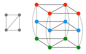
Figure 1: Left: The original graph to-be colored. Right: The qubit-layout encoding the problem. Each vertex $v$ is represented by $\kappa$ qubits $x_{v,c}$ for $c=1,\ldots\kappa$ representing its $\kappa$ possible colors. The extended graph construction can be thought of taking the graph represented in its natural Euclidean space and then augmenting that space with another dimension and replicating the graph $\kappa$ times for each of the colors. The phase separation Hamiltonian is composed of two-qubit operations corresponding to edges on each surface, and the mixing operation is among the qubits in the augmented dimension.

In the feasible subspace where each vertex is assigned exactly one color, the cost/objective function

$$f_{C}=m-\sum_{j=1}^{\kappa}\sum_{\{v,v^{\prime}\}\in E}x_{v,j}x_{v^{\prime},j}$$ (2)

counts the properly-colored edges, and we aim at maximizing $f_{C}$. By the replacement $x\to(\mathbf{1}-\sigma^{z})/2$ in Eq. (2), the corresponding quantum objective Hamiltonian is

$$H_{C} = \frac{1}{4}\Big{(}(4-\kappa)m\mathbf{1}+H^{\prime}_{C}\Big{)}\;,$$ (3)

where

$$H^{\prime}_{C} = \sum_{v=1}^{n}d_{v}\sum_{j=1}^{\kappa}\sigma^{z}_{v,j}-\sum_{j=1}^{\kappa}\sum_{\{v,v^{\prime}\}\in E}\sigma^{z}_{v,j}\sigma^{z}_{v^{\prime},j}\;.$$ (4)

Throughout this paper we use $\sigma_{x}$, $\sigma_{y}$, $\sigma_{z}$, and $X$, $Y$, $Z$ interchangeably to refer to the Pauli operators. The approximation ratio we will adopt in the following is the ratio of the expectation value of the cost Hamiltonian, projected onto the feasible subspace, to the true maximal number of correctly colored edges:

$$r=\frac{\langle P_{\mathrm{feas}}H_{C}P_{\mathrm{feas}}\rangle}{C_{\max}},$$ (5)

where $P_{\mathrm{feas}}$ is the projection operator onto the feasible subspace, and $C_{\max}$ is the number of edges in the true max-$\kappa$-colorable subgraph. Note that by projecting to the feasible subspace, the ratio of the feasible subspace to the full Hilbert space is also factored in. The numerator in Eq. (5) is equivalent to the average number of properly-colored edges observed upon measurement, with the infeasible output valued zero.

III.1 Adding a penalty in the phase separating Hamiltonian

The common practice for incorporate constraints is to add a penalty term to the cost function. For the one-hot-encoded problem we define a quadratic penalty to penalize the case that a node is assigned no color or multiple colors

$$f_{\text{pen}} = \sum_{v}(1-\sum_{j=1}^{\kappa}x_{v,j})^{2}$$ (6)

which, up to a constant, corresponds to the penalty Hamiltonian,

$$H_{\text{pen}} = \frac{1}{2}\sum_{v}\Big{(}(2-\kappa)\sum_{j}\sigma^{z}_{v,j}+\sum_{j<j^{\prime}}\sigma^{z}_{v,j}\sigma^{z}_{v,j^{\prime}}\Big{)}$$ (7)

that increases the energy of all states outside the subspace. The phase-separating Hamiltonian becomes a weighted sum of the cost and the penalty Hamiltonians

$$H_{\mathrm{PS}} = H^{\prime}_{C}-\alpha H_{\text{pen}}$$ (8)

where the weight parameter $\alpha\in\mathcal{R}_{+}$. Note that in Eq. (8) the penalty Hamiltonian is subtracted because we aim to maximize the original cost function and minimize the penalty. In order for the penalized function to have the same optima as the original cost function, the penalty weight needs to be set above a critical value. In the current problem, assigning more than one color to a vertex is not energetically favorable, so it is the opposite, assigning no color to a vertex that may create fake maxima. Since for every no-color vertex, there are at most $\lfloor d_{v}/\kappa\rfloor$ edges lifted from being improper, the penalty should satisfy $\alpha>\lfloor\max\{d_{v}\}/\kappa\rfloor$, we can loosely take $\alpha\geq n/\kappa$. On the other hand, the range of possible values of $f_{C}$ (and of spectral values of $H_{C}$) is $\kappa m$. Therefore, any $\alpha>\kappa m$ will ensure an energy separation between all feasible states and all infeasible states.

It should be noted that, unlike the motivating situation in adiabatic computation, the energy gap plays no clear role in QAOA. Thus it should be expected that, while the introduction of a penalty into the cost Hamiltonian may alter the QAOA dynamics, perhaps manipulating the reachable set of unitary operators, the role of the penalty strength is unclear at best. This perspective is supported by the numerical results in Section V.1. Indeed, while for some problems, such as the one-hot-encoded problems under consideration, sophisticated mixers can be designed to satisfy the constraints Hadfield et al. (2017), the design of general and systematic methods for incorporating constraints into QAOA remains an open problem.

In the penalty formulation the mixer can be either the standard $X$-driver

$$H_{X}=\sum_{v=1}^{n}\sum_{c=1}^{\kappa}\sigma^{x}_{v,c}\;$$ (9)

or the $XY$-Hamiltonian. If the $XY$-Hamiltonian is selected the penalty parameter may help the variational optimizer maintain probability mass in the feasible subspace and is not strictly necessary. In QAOA, it is unclear how a penalty parameter helps maintain probability mass over the feasible subspace. The feasible space of a $\kappa$-coloring problem is the set of states that satisfy

$$Z_{tot,v}\equiv\sum_{c=1}^{\kappa}\sigma^{z}_{v,c}=\kappa-2\;,$$ (10)

i.e., a subspace spanned by states in the computational basis that correspond to bit strings of Hamming weight equal to one.

Although formulating the penalty Hamiltonian facilitates the use of the standard $X$-mixer in QAOA, which can be implemented in constant circuit depth, we emphasize that the relative size of the feasible space becomes exponentially small as the graph size grows and thus a penalty formulation is sub-optimal. To see this, consider the size of the feasible subspace ${\cal H}_{\text{fea}}$; for each node, the feasible subspace can be spanned by states corresponding to $\kappa$ Hamming-weight one bit-strings, hence is of dimension $k$, and the feasible subspace for the whole problem is of dimension $k^{n}$. The ratio of the feasible subspace sizes to the size of the full Hilbert space is

$$\frac{\mathrm{dim}(\mathcal{H}_{{\text{f}ea}})}{\mathrm{dim}(\mathcal{H})}=\frac{\kappa^{n}}{2^{n\kappa}}=\big{(}\frac{\kappa}{2^{\kappa}}\big{)}^{n},$$ (11)

which for any $\kappa\geq 1$ shrinks exponentially with the graph size $n$.

III.2 $XY$ mixer: Enforcing evolution in the feasible subspace

The $Z_{tot,v}$ constraint can be incorporated in a natural way by selecting a mixing term that preserves the feasible subspace. Here we use the $XY$-Hamiltonian

$$H_{XY,v}=\frac{1}{2}\sum_{c,c^{\prime}\in K}^{\kappa}H_{XY,v,c,c^{\prime}}$$ (12)

$$H_{XY,v,c,c^{\prime}}=\sigma^{x}_{v,c}\sigma^{x}_{v,c^{\prime}}+\sigma^{y}_{v,c}\sigma^{y}_{v,c^{\prime}}\;.$$ (13)

which drives rotations in the $\{(0,1),(1,0)\}$ subspace of each color labeling. In the above equation the mixer applies to any color pair $c,\leavevmode\nobreak\ c^{\prime}$ in a set $K$. It can be verified that for any $K$, $[H_{XY,v},Z_{tot,v}]=0$.

III.2.1 Complete vs ring mixing Hamiltonians

In Eq. (12), when the mixing-set $K$ includes all pairs, the mixer is termed a complete-graph mixer. An alternative is the ring mixer in which $K$ takes a one-dimensional (1D) structure: $c^{\prime}=c+1$, and we apply periodic boundary condition. In the same fashion, there are a variety of derivative mixers based on the $XY$-Hamiltonian, depending on the underlying connectivity between colors. We focus on the complete-graph and ring mixers.

III.2.2 Simultaneous vs partitioned mixers

For a given mixing Hamiltonian, Eq. (12), for each node, a simultaneous mixer exactly applies the unitary $\exp[{-i\beta H_{XY,v}}]$ while a partitioned mixer applies the product of $\exp[{-i\beta H_{XY,v,c,c^{\prime}}]}$ in some order of $\{(c,c^{\prime})\}$. We define the parity-partition mixer such that a local $XY$-Hamiltonian is applied on even pairs first and odd pairs next.

The parity-partitioned mixing unitary is a first-order approximation of the simultaneous mixing unitary. Employing the Zassenhaus formula through second order

$$e^{it(H_{even}+H_{odd})}\approx e^{itH_{even}}e^{itH_{odd}}e^{\frac{t^{2}}{2}[H_{even},H_{odd}]}$$ (14)

allows us to characterize the leading error term $e^{-t^{2}/2[H_{even},H_{odd}]}$ as a function of $\kappa$. For simplicity, we consider even $\kappa$, so that $H_{even}$ and $H_{odd}$ contain $n/2$ commuting terms exactly. The parity-partitioned mixer can be represented as two separate Hamiltonians

$$H_{odd} = H^{(XY)}_{1,2}+H^{(XY)}_{3,4}+\ldots+H^{(XY)}_{\kappa-1,\kappa}$$

$$H_{even} = H^{(XY)}_{2,3}+H^{(XY)}_{4,5}+\ldots+H^{(XY)}_{\kappa,1}$$ (15)

where $H^{(XY)}_{j,j^{\prime}}=X_{j}X_{j+1}+Y_{j}Y_{j+1}$ and each term $H^{XY}_{j,j+1}$ in $H_{even}$ commutes with all terms in $H_{odd}$ except for $H^{(XY)}_{j-1,j}$ and $H^{(XY)}_{j+1,j+2}$. We can simply determine the term generated by the commutation

$$[H^{(XY)}_{j-1,j},H^{(XY)}_{j,j+1}]=2i(X_{j-1}Y_{j+1}-Y_{j-1}X_{j+1})Z_{j}$$ (16)

to obtain the general form of the error term. Therefore, $[H_{even},H_{odd}]$ is composed of $\kappa/2$ terms of type of Eq. (16). Since $||X_{j-1}Y_{j+1}Z_{j}||$ is of order $1$, we have $||[H_{even},H_{odd}]||\sim\kappa$ and therefore expect the difference between the simultaneous and the parity-partitioned mixing operators to be more prominent as $\kappa$ grows.

In the above analysis, the two mixing operators in general do not commute. However, we only need to focus on their effects in the feasible subspace. Here we provide analysis on the commuting relations in the feasible subspace for general $\kappa$. Note that each $H^{(XY)}_{j,j^{\prime}}$ operation in the feasible subspace corresponds to a $2\times 2$ permutation matrix. Then $H_{even}$ and $H_{odd}$ can be identified with the two permutations $\pi,\sigma\in S_{\kappa}$ on $\kappa$ letters:

$$\pi =\big{(}0\;1\big{)}\big{(}2\;3\big{)}\cdots\big{(}(\kappa-2)\;(\kappa-1)\big{)}$$ (17a)

$$\sigma =\big{(}1\;2\big{)}\big{(}3\;4\big{)}\cdots\big{(}(\kappa-3)\;(\kappa-2)\big{)}\big{(}(\kappa-1)\;0\big{)}.$$ (17b)

Thinking of the letters arranged on a circle, these are the two possible permutations that consist of $\kappa$ disjoint nearest-neighbor transpositions. It may be observed that

$$\sigma\pi=\big{(}0\;2\;4\;\dots\;(\kappa-2)\big{)}\big{(}1\;3\;5\;\dots\;(\kappa-1)\big{)}^{-1}$$ (18a)

is a product of two disjoint cyclic permutations and therefore is of order $\kappa/2$, i.e. $(\sigma\pi)^{\kappa/2}$ is the identity permutation. Now we see that $\pi$ and $\sigma$ satisfy exactly the relations necessary to generate $D_{\kappa}$, the dihedral group of order $\kappa$ Robinson (1995), i.e.,

$$D_{\kappa}=\langle\sigma,\pi|\sigma^{2}=\pi^{2}=(\sigma\pi)^{\kappa/2}=1\rangle.$$

In particular, we may note that, while $D_{4}$ is an abelian group (isomorphic to the Klein four-group $\mathbb{Z}_{2}\times\mathbb{Z}_{2}$), all $D_{\kappa}$ for $\kappa>4$ are non-abelian. Therefore only for $\kappa=4$, the simultaneous and the parity-partitioned ring mixers commute in the feasible subspace, hence are equivalent for QAOA.

III.2.3 Feasible initial states

The initial state in the standard QAOA framework with the $X$-mixer is $|+\rangle^{\otimes n}$, the even superposition over all bit strings, which is a fair starting point given no prior knowledge about the optimal solution. This state is also the ground state of the $X$-mixer, and can be generated by performing a single-qubit Hadamard transform on each qubit.

Under the new QAOA framework which accepts a constraint, the full space spanned by all bit strings $\{0,1\}^{n}$ is no longer a valid solution space. When the constraint, as in our case, dictates preserving the total magnetic quantum number,

$$Z_{tot,v}=\sum_{c=1}^{\kappa}\sigma_{c}^{z}=C$$ (19)

where $C\in[-\kappa,\kappa]$ is a constant integer, the feasible solution space is composed of Hamming-weight $(\kappa+C)/2$ bit strings, which correspond to states that satisfy Eq. (19). In analogy to the $|+\rangle^{\otimes n}$ state for the case where all bit strings are feasible solutions, a fair initial state should be the even superposition of all Hamming-weight $(\kappa+C)/2$ bit strings. Such a state is also an eigenstate of the $XY$ mixer. In the graph coloring problem, $C=\kappa-2$, the generalized $W$-state is the fair starting state. In section C we survey circuit construction methods that can be used to create a $W$-states.

IV Circuit realizations

In this section we describe how to implement the various components of QAOA into short depth circuits. We start by assuming the physical qubits are all-to-all connected, and show that the simultaneous complete-graph and ring mixers can be realized in depth linear and logarithmic in $\kappa$, respectively. In Sec. IV.3 we discuss the depth required due to limited connectivity between the physical qubits.

IV.1 Logarithmic depth simultaneous ring mixer

Interacting spin-1/2 chain is one of the oldest problems of quantum mechanics. Stemming from the resemblance between spin-1/2 raising (resp. lowering) operators and fermionic creation (resp. annihilation) operators, in a detailed work of [Jordan and Wigner, 1928], the Jordan-Wigner transformation was introduced to convert spin-1/2 systems into problems of interacting spinless fermions. While in general spin-spin interactions map to non-local fermionic interactions, for the one-dimensional $XY$ problem the transformation results in a particularly precise form involving only quadratic fermionic couplings:

$$H_{XY}= \sum_{c=1}^{\kappa}\left(\sigma_{c}^{x}\sigma_{c+1}^{x}+\sigma_{c}^{y}\sigma_{c+1}^{y}\right)$$

$$\downarrow$$

$$H_{XY}= 2\sum_{c=1}^{\kappa}\left(a_{c}^{\dagger}a_{c+1}+\mathrm{h.c.}\right)\;,$$ (20)

where $\hat{a}$ and $\hat{a}^{\dagger}$ are fermionic operators, and we assumed $\kappa$ is even for simpler demonstration.

The quadratic Hamiltonian in Eq. (20) can be diagonalized by a basis rotation on the operators. For nearest-neighbor, one-body coupling, the fermionic Fourier transform

$$\hat{a}_{c}^{\dagger} =\mathrm{FFFT}^{\dagger}\hat{f}_{k}^{\dagger}\mathrm{FFFT}\equiv\frac{1}{\sqrt{\kappa}}\sum_{c}e^{i2\pi ck}\hat{f}_{k}^{\dagger}$$ (21)

$$\hat{a}_{c} =\mathrm{FFFT}^{\dagger}\hat{f}_{k}\mathrm{FFFT}\equiv\frac{1}{\sqrt{\kappa}}\sum_{c}e^{-i2\pi ck}\hat{f}_{k}\;,$$

is sufficient to diagonalize the Hamiltonian. We use the notation $\rm FFFT$ (fermionic fast Fourier transform) to denote the circuit for the operator Fourier transform and not the quantum Fourier transform Babbush et al. (2017). The $XY$ Hamiltonian on a ring is then exactly diagonalized asLieb et al. (1961)

$$H_{XY} = \sum_{k=1}^{\kappa}E_{k}f_{k}^{\dagger}f_{k}$$ (22)

where the eigen-energies $E_{k}=2\cos(2k\pi/\kappa)$. Replacing the number operator $f_{k}^{{\dagger}}f_{k}$ with qubit operators $(1-\sigma_{k}^{z})/2$, the Hamiltonian can be expressed as

$$H_{XY}^{(k)}=\sum_{k=1}^{\kappa}E_{k}\left(1-\sigma_{k}^{z}\right)/2\;\;$$ (23)

where the upper index $(k)$ is added as a reminder that we are in the momentum representation. In this representation evolving $e^{-i\beta H^{(k)}_{XY}}$ involves only single-qubit $Z$-rotations.

The FFFT has emerged as a route to efficient simulation for fermions in tensor networks Ferris (2014) and quantum circuits representing fermionic systems Verstraete et al. (2009); Babbush et al. (2017). The circuit is constructed in a similar structure to the decimation-in time radix-2 classical Fourier transform and inherits the divide-and-conquer complexity. The FFFT circuit can be implemented with $\mathcal{O}(\mathrm{log}(\kappa))$ Ferris (2014) depth for a system with parallel arbitrary two-qubit interactions. For more realistic systems where only nearest-neighbor interactions are allowed fermionic swaps are required to swap the two modes together to perform the butterfly operation. This adds an additional overhead resulting in a $\mathcal{O}(\kappa\mathrm{log}(\kappa))$ circuit depth and $\mathcal{O}(\kappa^{2}\mathrm{log}(\kappa))$ total gate count Babbush et al. (2017). The gate depth required to implement the FFFT was further improved to $O(\kappa)$ in  Kivlichan et al. (2018) by using a Givens rotation network and requires only linear connectivity.

We also point out that the Givens rotation network is a powerful tool for state preparation for general quadratic Hamiltonians. For pairing models, the linear depth network was used to prepare ground states Jiang et al. (2018). This initial state can be used in the context where the hard constraint is of the form that qubits must appear paired up. We point this out as an example of how different flavor constraints can correspond to evolving a wide variety of constraint-preserving Hamiltonians.

IV.2 Linear depth simultaneous complete-graph mixer

We consider the simultaneous mixer for a node, $e^{-i\beta H_{{\tt complete}},v}$, with $H_{{\tt complete},v}=\sum_{c<c^{\prime}=0}^{\kappa-1}H_{XY,v,c,c^{\prime}}$, which corresponds to a complete graph of variables corresponding to all colors for each vertex $v$, $\{x_{v,c}\}$. Beyond a one-dimensional layout, the analytical solution to the $XY$ model is not known, therefore, exactly realizing the evolution of $XY$ model on a complete graph poses a challenge. In this section we show that within the subspace of total $Z_{tot,v}=\pm(\kappa-2)$ as in our case, when $\kappa=2^{m}$, this unitary can be exactly implemented in a circuit of depth $\kappa-1$, up to a constant factor accounting for breaking a generic two-qubit operator to any fixed universal set of single- and two-qubit operators.

We illustrate the process using $\kappa=4$ and then show the general formula. For $\kappa=4$, we consider three partitions of the full set of colors: $\{\{0,1\},\{2,3\}\}$, $\{\{0,2\},\{1,3\}\}$ and $\{\{0,3\},\{1,2\}\}$, in the feasible subspace, we have

$$\exp[-i\beta\sum_{c,c^{\prime}\in[0,3]}{(XY)}_{c,c^{\prime}}]=$$

$$\exp[-i\beta\big{(}{(XY)}_{0,1}+{(XY)}_{2,3}\big{)}]$$

$$\exp[-i\beta\big{(}{(XY)}_{0,2}+{(XY)}_{1,3}\big{)}]$$

$$\exp[-i\beta\big{(}{(XY)}_{0,3}+{(XY)}_{1,2}\big{)}]\;,$$ (24)

where for notational simplicity we use $(XY)_{j,j^{\prime}}$ to refer to the XY Hamiltonian $H^{(XY)}_{j,j^{\prime}}$ defined below Equation (15). Note that this equivalence is approximate in general but exact if we consider only the action on the feasible subspace. The fact that these partitioned operators commute in the feasible subspace can be easily verified mathematically.

The following perspective on the partitioning scheme allows us to derive a generalization for any $\kappa$. Consider an integer variable $x\in\{0,1,2,3\}$, in the one-hot encoding, in the feasible space, the $XY$ operation on a pair of qubits swaps the integer values the states represent. For example $(XY)_{1,3}$ swaps between the variable taking value $1$ and taking value $3$. Now consider the $2$-bit binary encoding of $x$: $x=2^{1}x_{1}+2^{0}x_{0}$ where $x_{0}$ and $x_{1}$ are bits. The swap between $\{0,1\}$ and $\{2,3\}$ corresponds to flipping the zero-th bit $x_{0}$. The swap between $\{0,2\}$ and $\{1,3\}$ corresponds to flipping the first bit $x_{1}$. The swap between $\{0,3\}$ and $\{1,2\}$ corresponds to flipping both bits $x_{0}$ and $x_{1}$. Such operations can happen in any order without affecting the final value of $x$, hence the corresponding partitioned mixers commute.

For a general $\kappa=2^{m}$, the partition can be read out taking the inverse of this process: all pairs involved in each $l$-bit flipping form a partition, for $l=1,\ldots,m$. There are $\binom{m}{l}$ many $l$-bit flips, hence the total partitions $\sum_{l=1}^{m}\binom{m}{l}=2^{m}-1=\kappa-1$. Within each partition the pair-wise $XY$ operators commute and can be executed simultaneously. The simultaneous complete-mixer unitary can be accordingly executed in depth $\sim\kappa-1$.

For example, partitions for $\kappa=8$ can be prescribed using the following equations. Here we use $\tilde{0},\tilde{1},\tilde{2}$ to represent bits in the binary encoding. The left-hand side for each equation is a $l$-bit flip operation, all seven operations commute. The right hand side is derived from reading off the effect of the operation on the numerical colors. The right-hand side gives the corresponding partition for the $XY$ operators in the one-hot encoding, with the detailed procedure displayed in Table. 1.

$$I_{\tilde{2}}I_{\tilde{1}}X_{\tilde{0}} = (XY)_{01}+(XY)_{23}+(XY)_{45}+(XY)_{67}$$

$$I_{\tilde{2}}X_{\tilde{1}}I_{\tilde{0}} = (XY)_{02}+(XY)_{13}+(XY)_{46}+(XY)_{57}$$

$$X_{\tilde{2}}I_{\tilde{1}}I_{\tilde{0}} = (XY)_{04}+(XY)_{15}+(XY)_{26}+(XY)_{37}$$

$$I_{\tilde{2}}X_{\tilde{1}}X_{\tilde{0}} = (XY)_{03}+(XY)_{12}+(XY)_{47}+(XY)_{56}$$ (25)

$$X_{\tilde{2}}I_{\tilde{1}}X_{\tilde{0}} = (XY)_{05}+(XY)_{14}+(XY)_{27}+(XY)_{36}$$

$$X_{\tilde{2}}X_{\tilde{1}}I_{\tilde{0}} = (XY)_{06}+(XY)_{17}+(XY)_{24}+(XY)_{35}$$

$$X_{\tilde{2}}X_{\tilde{1}}X_{\tilde{0}} = (XY)_{07}+(XY)_{16}+(XY)_{25}+(XY)_{34}$$ (26)

$decimal$	one-hot	Apply IXX	decimal
0	000	011	3
1	001	010	2
2	010	001	1
3	011	000	0
4	100	111	7
5	101	110	6
6	110	110	5
7	111	100	4

Table 1: Demonstration of deriving the partition corresponding to operator $IXX$ on the binary encoding, Eq. (25)

.

IV.3 On realistic layout of physical qubits

To achieve the above derived circuit depth for simultaneous ring and complete-graph mixers requires physical qubits to have a particular connectivity. For example, all-to-all connectivity for the simultaneous complete-graph mixer. For a physical-qubit-layout of lower connectivity, SWAP operations may be necessary to enable the pairwise operations Venturelli et al. (2018); Guerreschi and Matsuura (2019).

We first note that in the feasible space, an $XY$ operation $\exp[-i\beta(XY)_{j,j^{\prime}}]$ and a SWAP${}_{j,j^{\prime}}$ executed consecutively are equivalent to a $XY$ of different parameter:

$$e^{-i\beta(XY)_{j,j^{\prime}}}\text{SWAP}_{j,j^{\prime}}=ie^{-i(\beta+\frac{\pi}{2})(XY)_{j,j^{\prime}}}\;.$$ (27)

or, in matrix form

$$\begin{pmatrix}1&0&0&0\\ 0&-i\sin{\beta}&\cos{\beta}&0\\ 0&\cos{\beta}&-i\sin{\beta}&0\\ 0&0&0&1\\ \end{pmatrix}$$ (28)

This relation can be explored in circuit compilation to achieve a circuit on physical qubits of lower depth.

For example in the $\kappa=4$ example for simultaneous complete-graph mixer in Sec. IV.2 if the physical qubits form a ring $1-2-3-4-1$, the three partitions can be executed in the following order:

$$\{\{0,1\},\{2,3\}\}$$

$$\{\{0,3\},\overline{\{1,2\}\}}$$

$$\{\{0,2\},\{1,3\}\}$$

where the pair with an overline indicates a SWAP is combined in the $XY$ mixing in the fashion of Eq. (27). This SWAP enables the operation of the last partition, and the whole circuit is of depth $3$, the same as in the case of a complete graph.

For a general $\kappa$ simultaneous mixer, this feature helps scheduling but cannot avoid SWAPs completely because the partitions need to be executed in a specific order.

On the other hand, executing the pairwise $XY$ unitary in any given order would give a valid partitioned mixer, though not equivalent to the simultaneous one. Exploiting the feature Eq. (27) combined with a bubble sort scheme, we can completely avoid SWAPs and implement a partitioned complete-graph mixer in linear depth.

The same SWAP network circuit architecture, derived from a fermionic simulation perspective, can be used to implement the phase-separator Hamiltonian with no Trotter error Kivlichan et al. (2018); Crooks (2018). Viewing the qubits as an array of $\kappa$-sites the parallel bubble sort algorithm implements a swap network in $\kappa$-depth where every element (qubit) of the array is swapped passed each other once.

Since all terms in the phase-separator commute, there is no incurred Trotter error. The swap interaction can be efficiently combined with the evolution of a $e^{-i\theta ZZ}$ nearest-neighbor interaction by adding an $e^{-i\theta Z}$ in between the second and third CNOT (denoted CX below) in the SWAP decomposition Venturelli et al. (2018).

Explicitly,

$$\mathrm{SWAP}_{0,1}e^{-i\theta ZZ_{0,1}}= \mathrm{CX}_{0,1}\mathrm{CX}_{1,0}\mathrm{CX}_{0,1}e^{-i\theta ZZ_{0,1}}$$ (29)

$$= \mathrm{CX}_{0,1}\mathrm{CX}_{1,0}.e^{-i\theta Z_{1}}\mathrm{CX}_{0,1}$$ (30)

can be used as the swap interaction and simultaneously evolve a local $ZZ$-interaction term. For any encoding model that increases the dimensions of the graph, such as in the case where one-hot-encoding is used, simulating the interaction term removes the necessity of encoding techniques such as minor embedding or classical logical encoding Lechner et al. (2015); Rocchetto et al. (2016).

V Simulation Results

In this section, we present the results of numerical simulations of QAOA applied to the max-$\kappa$-Colorable-Subgraph problem. We first compare the performance of the $XY$ mixer to that of the $X$ mixer with penalty. We then more deeply explore the behavior of $XY$ mixers, looking at general features of their performance on small hard-to-color graphs, and comparing complete-graph $XY$ mixers against ring $XY$ mixers.

To acquire a good set of QAOA parameters, stochastic optimizer is needed, in Appendix. B we show rugged landscape with local optima in the parameter space that would cause problem for deterministic optimizing methods like gradient descend. We instead use basin-hopping with Broyden-Fletcher-Goldfarb-Shanno (BFGS) algorithm to obtain (sub)optimal parameters.

V.1 The death of $X$-mixer

We use a simple example, 2-coloring and 3-coloring of a triangle to demonstrate the performance comparison of $XY$ and $X$ mixers.

Note that the penalty weight $\alpha$ in general affects the performance of the algorithm. In Fig. 2 we show that for 2-coloring the approximation ratio optimized over the parameter set $(\gamma,\beta)$ for each penalty weight $\alpha$. The best approximation ratio, $r$, takes value $0.75$ while with $XY$ driver QAOA_p=1 gets $r=1$.

In Fig. 2, while the penalty strength has an effect on the behavior of level 1 QAOA, there appears to be no clear intuition for choosing a good value. In particular, the minimum penalty that guarantees the optimal state being the optimal state in the feasible subspace, indicated by the red arrows on the plots, does not stand out, nor does the penalty value that guarantees separation between energies feasible and infeasible states, indicated by the the blue arrows. This supports our argument in Sec. sec:penalty that the role of energy gap plays no clear role in QAOA.

For 3-coloring, in Fig. 3b we plot how the approximation ratio varies in the 2-dimensional $(\gamma,\beta)$ space, for using the $X$ mixer and for using the $XY$ mixer. While with the $X$ mixer the QAOA_p=1 gives approximation ratio $\sim 0.2$ across the parameter value range, with the $XY$ mixer parameter values that correspond to $\sim 0.8$ can easily be found. This example thus shows significant performance advantage in using the $XY$ as compared with the $X$ mixer.

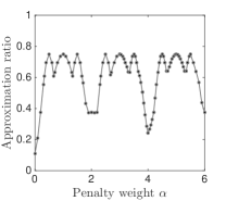
(a)

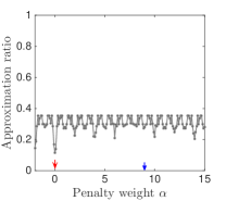
(b)

Figure 2: (a) 2-coloring (b) 3-coloring of triangle with level 1 $\mathrm{QAOA}$. The highest approximation ratio across the parameter sets ($\gamma_{1},\beta_{1}$) is plotted versus the penalty weight $\alpha$. The red arrow at $\alpha=0$ indicates the minimum penalty that guarantees the optimal state being the optimal state in the feasible subspace, and the blue arrow at $\alpha=9$ indicates the penalty value that guarantees separation between energies feasible and infeasible states.

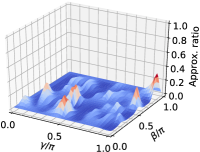
(a)

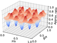
(b)

Figure 3: Numerical results for level 1 $QAOA$ on the problem of 3-coloring of a triangle graph. (a) using $X$ mixer along with phase-separating Hamiltonian, Eq. (8) where the penalty weight is taken to be the numerically determined optimal value $\alpha^{*}=1.7$.

(b) using the $XY$ mixer with W-state being the initial state.

V.2 Small and hard-to-color graphs

For a fixed classical algorithm, a slightly-hard-to-color graph is a graph for which the algorithm will sometimes yield the optimal solution. Similarly, a hard-to-color graph is one such that the chosen algorithm never yields the optimal solution. Two examples are the Envelope and the Prism graphs,Kosowski and Manuszewski (2008) sketched in Figure. 4. The Prism graph is the smallest slightly-hard-to-color graph for the smallest-last(SL) sequential coloring method and the Envelope graph is the smallest hard-to-color graph for the largest-first(LF) sequential method. Note that these classical algorithms are aiming to compute the chromatic number, while in this paper we focus on finding the maximal colorable subgraph. Although finding the max-colorable subgraph could serve as a subroutine for determining chromatic numbers, the chromatic number can also be directly attacked by QAOA using a much more complex mixer.Hadfield et al. (2017) Nevertheless we are not aiming at doing side-by-side comparison of quantum and classical algorithms, and will use these small graphs only as a proof-of-principle demonstration of the QAOA with $XY$ mixers.

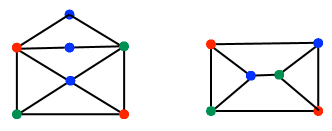
Figure 4: The two small and hard-to-color graphs: Envelope and Prism. A valid 3-coloring is shown on each graph.

V.2.1 Performance of QAOA with the simultaneous ring mixer

With the simultaneous ring mixer, Figure. 5 shows the results for QAOA levels 1 to 6. For each level, the W-state is used as initial state, and stochastic search (basin-hopping with BFGS) is performed to optimize the expected value of the cost Hamiltonian over the angle sets. The approximation ratio corresponding to the optimal expectation value is plotted as filled circles. Even at level one, the approximation ratio takes a high value 0.8, and this value quickly approaches 1 as the level increases. Furthermore, for each level, we computed the probability of getting the actual optimal solution (a valid 3-coloring) upon measurement. At level one, this probability is slightly lower than 0.2, and quickly goes above 0.6 at level-3, which implies that repeating the experiment 3 times, one will find a valid coloring with probability $>0.9$.

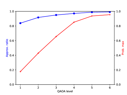
Figure 5: The Prism graph. Dots are approximation ratios and crosses are the expected probability of getting the optimal coloring. For each QAOA level, results are shown at the (sub)optimal angles resulted from a basin-hopping search.

V.2.2 Effect of initial states

The W-state – as both an even superposition of all feasible classical states, and the ground state of the simultaneous ring mixer – is a natural candidate for the initial state for QAOA. It involves multiple two-qubit gates to prepare. An easier-to-prepare state for each vertex can be defined via a randomly-assigned coloring (feasible but not necessarily optimal), $|\psi_{C}\rangle$, i.e., a randomly drawn bit string of Hamming weight one. Preparing such a state involves only $n$ single-qubit gates.

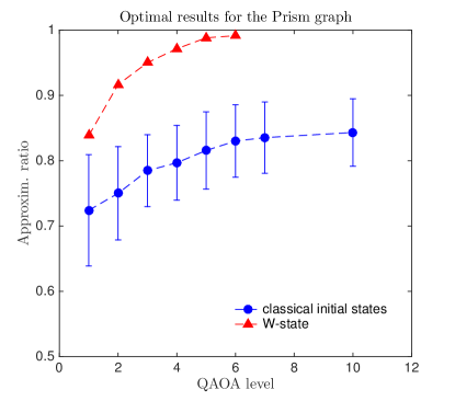
Figure 6: The Prism graph, the expected value of QAOA optimized over the angle sets. Triangles show the results with W-state as initial states. Circles show the results with a feasible classical initial state, averaged over the set of all feasible classical states, the error bar is the standard deviation. For each initial state, optimization over angles are derived from a basin-hopping search.

We study both initial states for the prism graph with simultaneous ring mixer. For level-1 QAOA, the best achievable optimization ratio (optimized over all angle sets $(\beta,\gamma)$) for W-state is higher than the classical Hamming weight 1 state $|\psi\rangle_{C}$. Notice that for $|\psi\rangle_{C}$, the phase-separating unitary commutes with the density matrix of the state, hence has no effect to the state evolution. As a result, the whole circuit for level-1 QAOA is equivalent to applying the mixing unitary followed by measurement. We further simulated higher levels, and in Figure. 6 show the performance of QAOA with the W-state versus a classical state as initial state. We found that with the classical initial state, the performance of QAOA is significantly lower than using the W-state as initial state. Even at level 10, $r_{classical}$ is still lower than $r_{W}$ for level-1. Moreover, the approximation ratio with classical initial state shows a tendency toward saturation around level 10 – this could either be the nature of the algorithm, or due to increasing difficulty in finding the global optimum in the parameter subspace as the level increases, which poses another practical consideration for application. (Note that due to the optimization over parameter space for each initial state, the average over classical initial state is not equivalent to prepare the initial state in a mixed state for the ensemble).

Because our simulation is noise-free, due to ergodicity, in the limit of $p\to\infty$ the optimal performance should be independent of the initial state. But for practical implementation on a near-term hardware where noises accumulates fast with circuit depth, such medium-level QAOA behavior is of high relevance. In Appendix C we survey methods to generate quantum circuits for preparing W-states. It is shown that with certain methods it can be generated with $O(\kappa)$ CNOT gates. The overall performance of QAOA will be a tradeoff between the extra effort in preparing W-state and the damage that comes with circuit depth.

V.3 Benchmarking graph sets

To better understand the behavior of these QAOA graph-coloring algorithms, we make use of the sets of all $\kappa$-chromatic graphs of size $n$ as the benchmarking sets for the $XY$ mixers under consideration. See Table 2 for the number of instances in each benchmarking set.

$\chi$	$n$	No. graphs
3	5	12
3	6	64
3	7	475
4	6	26
4	7	282
5	7	46
6	7	5

$n$	$\kappa$	No. graphs
4	4	6
4	6	6
4	8	6

Table 2: Left: Benchmarking graph sets: each row indicates all $\chi$-chromatic graphs of size $n$, and we solve the problem of $\kappa$-coloring of such graphs choosing $\kappa=\chi$. Right: Benchmarking graph sets II for examining the simultaneous vs partitioned ring mixers on different ring sizes: Each row indicates all connected graphs of size $n$, and we solve the problem of $\kappa$-coloring of such graphs. Because the total number of qubits is $n\kappa$, which is the limiting factor to the simulation, we limit to small $n$ to see $\kappa$ varying up to $8$.

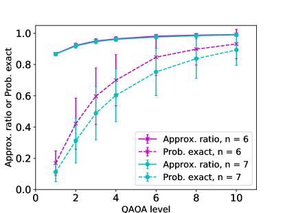
Figure 7: Approximation ratio (solid lines) and probability to exact solution (broken lines) for QAOA with ring simultaneous mixer. $n=6$ (crosses) vs $n=7$ (filled circles).

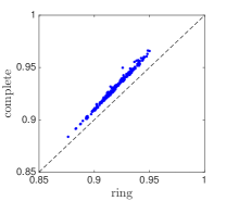
(a) QAOA level-2

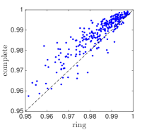
(b) QAOA level-8

Figure 8: QAOA with simultaneous mixers. Performance comparison between ring and complete-graph mixers applied to the same graph coloring problems. The axes show approximation ratio achieved using the labeled mixer type. Scatter plot shows the results for $4$-coloring of all connected chromatic-$4$ graphs of size $n=7$. In (b), for better visibility, an outlier data point at (ring = 0.95, complete = 0.9) is not shown in the plot.

V.3.1 Approximation ratio and probability-to-optimal-solution

Using $W$-state as the initial state, for simultaneous ring and complete-graph mixers, the mean and median of the approximation ratio as well as the probability-to-optimal-solution is evaluated across problem sets.

The following observations have been made on the typical performance for each problem set.

Consistent performance over instances.

For all problem sets, the approximation ratio and the probability-of-optimal-solution curves as a function of the QAOA level are highly consistent across graphs, bearing the same shape for the Prism and Envelope graphs. For each problem set, the approximation ratio showed very little deviation from the mean (demonstrated by the small error bars in Figure. 7).

Larger graphs are harder to color.

As expected, for the same $\kappa$, as $n$ increases, the performance of QAOA with the same type of mixer decreases, see Figure. 7 for comparison of the simultaneous ring-mixer for $n=6$ and $n=7$.

Complete-graph mixer is better than the ring mixer.

For the same problem size $n$, the simultaneous complete-graph mixer demonstrates better performance than the simultaneous ring-mixer in QAOA levels from 1 to 10. See the scatter plot for QAOA level-2 and level-8 in Figure 8. For small QAOA levels, this advantage is uniform cross instances for smaller levels, as shown in Figure 8 (a) for level-2 where for all 282 instances the complete mixer generates higher approximation ratio. The advantage is decreasing as QAOA level increases, see comparison of (a) and (b). This is possibly due to the approximation ratio getting close to 1. We also speculate that the QAOA level where this closeup happens would vary with, $\kappa$, the number of colors.

Similar performance between the simultaneous and parity mixers for small $\kappa$.

We also study $\kappa$-coloring of all connected graphs (regardless of chromatic number) of size $n=3,\leavevmode\nobreak\ 4$, with varying $\kappa$ to compare simultaneous vs partitioned ring mixers on different ring sizes. Since for $\kappa=4$, the simultaneous and the parity mixers are equivalent, we will need to go for higher $\kappa$ to examine the difference, however, numerical power is limited by the number of qubits $n\kappa$, we thus examined two classically trivial cases, $n=4,\leavevmode\nobreak\ \kappa=6$ and $8$ (trivial coloring exists). Both approximation ratio and probability of exact solution are high due to the small problem size, and no noticeable difference is observed between the performance of partitioned and simultaneous mixers. Extensive studies on larger problem sizes are needed to further evaluate these two types of mixers.

V.3.2 Typical solution upon measurements

Note that our optimization over the set of angles is designed to maximize the expected value, and the high approximation ratio discussed in Section V.3.1 is also about the expected value. For approximate optimization, the expectation value of the approximation ratio is not the whole story. One also cares about the probability of getting the optimal or near-optimal states upon measurement. We apply the argument and analysis on the tail probability in Sec. II, Eq. (1), on the case of $3$-coloring of the Envelope graph (11 edges), and show in Figure 9 the theoretical lower bound in probability of getting a solution with costs $10$ or $11$, i.e., the valid coloring or only one improperly-colored edges. The true probability from evaluating the wavefunction is shown for comparison. For QAOA level three and up, the bound inferred from the approximation ratio gives us confidence that with greater than $50\%$ probability we will get the optimal or the next best solutions.

Viewing the QAOA as an exact solver, as observed in the case of small hard-to-color graphs, for the benchmarking problem sets, we also see that as $p$ increases, along with the increase in $r^{*}$, there is a more drastic increase in the probability of getting a optimal solution. In Fig. 7 we also plot the mean prob-to-optimal-solution as $p$ changes, with error bars indicating the standard deviation over the graphs in the set.

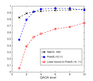
Figure 9: $3$-coloring of Envelope graph (11 edges). QAOA with simultaneous ring-mixer. For each QAOA level, the probability of getting the top two highest approximate results (cost 11 and 10) is shown in comparison to the bound given by Eq. (1) with the observed approximation ratio as parameter.

VI Conclusion

Exploring the range of applications of the QAOA provides insight into what can be achieved with near-term quantum resources. While the general search for applications of QAOA is important, the detailed specification of the algorithm can be the difference between success and failure when running the algorithm on a real device. These details can change if the gate-model computing substrate is switched–e.g. switching from superconducting qubits to ions. For example, constant factors in circuit depth gained by switching gate sets can drastically change circuit depth and thus the success probability of the overall algorithm.

In this work we explored applying QAOA to optimization over $\kappa$-ary variable sets. Our representative example of this optimization was the max-$\kappa$-colorable-subgraph problem on small hard-to-color graph problems. We numerically demonstrate and theoretically motivate that the $XY$-mixer Hamiltonian is a natural choice for this particular set of problems. Part of the numerical analysis was providing circuit implementations for the phase-separator and the $XY$-mixer under various qubit topologies. Though there is higher implementation cost of the $XY$-mixer in comparison to the standard $X$-mixer, the benefits of eliminating a penalty term and restricting dynamics to the feasible space can potentially outweigh the linear-depth implementation cost.

Along with the circuit analysis the bound on tail effects based on the mean value we provide in Eq. (1) suggests that a high mean value is sufficient to guarantee performance without having to analyze the variance of the distributions produced by QAOA.

This work establishes the possibility of using more sophisticated drivers in a QAOA framework for naturally including constraints. We expect this analysis is helpful for near-term experimental validations of the QAOA algorithm and, hopefully, inspires alternative constraint encodings that would lower the representational cost of real-world optimization problems.

VII Acknowledgements

ZW thank enlightening discussions with all Quail members, Zhang Jiang, and Sergey Knysh. We are grateful for support from NASA Ames Research Center, and from the NASA Advanced Exploration systems (AES) program and the NASA Transformative Aeronautic Concepts Program (TACP), and also for support from the AFRL Information Directorate under grant F4HBKC4162G00. ZW is also supported by NASA Academic Mission Services (NAMS), contract number NNA16BD14C.

Appendix A Proof on finite tail probabilities

In what follows, we will take $\{a_{j}\}_{j=0}^{K}\subset\mathbb{R}$ to be a strictly ordered finite set, i.e. $a_{0}<a_{1}<\dots<a_{K}$. Suppose that $p_{j}$ is the probability of a random variable $X$ having outcome $a_{j}$, with $\sum_{j=0}^{K}p_{j}=1$. We will assume below that we know the values $\{a_{j}\}$ and the mean $\mu$ of this probability distribution, but not the entire distribution itself.

Lemma 1.

Given $\mu=\sum_{j=0}^{K}p_{j}a_{j}$, with $\mu\geq a_{l}$ for some $0\leq l\leq K$,

$$\Pr(X>a_{l})\geq\frac{\mu-a_{l}}{a_{K}-a_{l}}=1-\frac{a_{K}-\mu}{a_{K}-a_{l}}.$$ (31)

Proof.

We will prove the bound using the method of Lagrange multipliers. To ensure the probabilities are nonnegative, we will represent them as squares: $p_{j}=q_{j}^{2}$. Then the Lagrangian is

$$\mathcal{L}=\sum_{j=l+1}^{K}q_{j}^{2}+\lambda\left(\sum_{j=0}^{K}q_{j}^{2}-1\right)+\gamma\left(\sum_{j=0}^{K}q_{j}^{2}a_{j}-\mu\right).$$ (32)

Differentiating and setting the derivatives equal to zero, we find the conditions

$$2q_{j}\left(\delta_{>l}(j)+\lambda+a_{j}\gamma\right)=0,$$ (33)

i.e.,

$$\text{for }j\leq l: q_{j} =0\qquad\text{or} \lambda+a_{j}\gamma=0$$ (34a)

$$\text{for }j>l: q_{j} =0\qquad\text{or} 1+\lambda+a_{j}\gamma=0.$$ (34b)

First, consider the case that $q_{j}=0$ for all $j>l$. Then $p_{j}=q_{j}^{2}=0$ for all $j>l$, so the only way $\mu\geq a_{l}$ can be satisfied is if $\mu=a_{l}$. Then $\Pr(X>a_{l})=\sum_{j=l+1}^{K}p_{l}=0=\frac{\mu-a_{l}}{a_{K}-a_{l}}$, so (31) is satisfied. Similarly, if $q_{j}=0$ for all $j\leq l$, then $\Pr(X>a_{l})=1$, so this case represents the maximum, rather than the minimum of $\Pr(X>a_{l})$, and in any case, (31) is satisfied.

Now, if $q_{m}\neq 0$ and $q_{n}\neq 0$ for $0\leq m<n\leq l$, then it follows that $\lambda=\gamma=0$ and therefore $q_{j}=0$ for all $j>l$, so that, as just argued, (31) is satisfied. If, on the other hand, $q_{m}\neq 0$ and $q_{n}\neq 0$ for $l<m<n\leq K$, then it follows that $\gamma=0$ and $\lambda=-1$, so that $q_{j}=0$ for all $0\leq j\leq l$, and therefore , (31) is satisfied.

What remains is the case that exactly one $q_{m}\neq 0$ for $0\leq m\leq l$ and exactly one $q_{n}\neq 0$ for $l<n\leq K$ and all other $q_{j}$ are zero. Then $\Pr(X>a_{l})=p_{n}$, $p_{m}=1-p_{n}$ and $\mu=p_{m}a_{m}+p_{n}a_{n}=(1-p_{n})a_{m}+p_{n}a_{n}$. Solving for $p_{n}$, we find

$$\Pr(X>a_{l})=p_{n}=\frac{\mu-a_{m}}{a_{n}-a_{m}}=1-\frac{a_{n}-\mu}{a_{n}-a_{m}}.$$ (35)

It is easily seen that this expression for $p_{n}$ decreases as $a_{n}$ increases and decreases as $a_{m}$ increases, so the minimum $p_{n}$ obtained in this way is when $m=l$ and $n=K$:

$$\Pr(X>a_{l})=p_{n}=\frac{\mu-a_{l}}{a_{K}-a_{l}}=1-\frac{a_{K}-\mu}{a_{K}-a_{l}},$$ (36)

from which it follows that (31) is satisfied. ∎

Appendix B Rugged landscape

The landscape of the parameter space plays an important role in quantum control. In the case of MaxCut for a ring graph (equivalent to binary encoding for a 2-coloring of the ring), in Ref. Wang et al. (2018) it has been observed that the landscape contains only global maximum. In the current case of QAOA with $XY$ driver on graph coloring, we notice that even for level-1 QAOA, the control landscape is rugged and contains local maximum. In Fig. 10 the landscape for the Envelope graph is plotted, and the bottom panel reveals local optima. Stochastic optimization is therefore needed to perform parameter search.

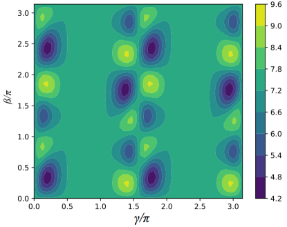
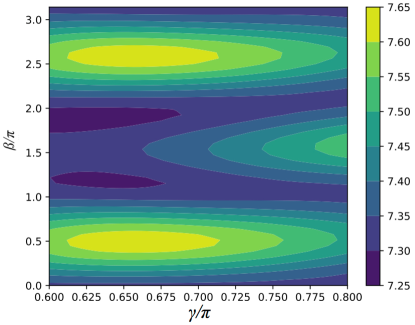
Figure 10: Landscape for level-1 QAOA for the envelope graph. Top: Full landscape. Bottom: Zoom-in of the seemingly flat area that contains local maxima.

Appendix C W-state generation

The $W$-state is a well-known multipartite-entangled state that plays an important role in quantum information theory. Here, we survey methods to produce a generalized W-state using quantum gates.

C.1 Sequential generation of W-state

In Ref. Schön et al. (2007), it was shown a W-type state, which is any state living in the subspace spanned by states corresponding to Hamming-weight-1 bit strings, can be generated using an auxiliary qubit by sequentially entangling it with each qubit. Here we detail the case for the W-state using this method. Consider an auxiliary qubit $q_{0}$ and an $n$-qubit register ($q_{1}$ to $q_{n}$), initialized in the tensor product state $|0\rangle\otimes{|0\rangle}^{\otimes{n}}$. Entanglement between $q_{0}$ and $q_{j}$ is introduced by unitary

$$U_{0,j}(\theta_{j},\phi_{j}) =|01\rangle\langle 01|+|10\rangle\langle 10|$$

$$+c_{j}|00\rangle\langle 00|+c_{j}|11\rangle\langle 11|$$

$$+s_{j}|11\rangle\langle 00|-s^{*}_{j}|00\rangle\langle 11|\;,$$ (37)

where $c_{j}\equiv\cos\theta_{j}$ and $s_{j}\equiv e^{i\phi_{j}}\sin\theta_{j}$. This unitary generates superposition between $|00\rangle$ and $|11\rangle$ state in the subspace of $q_{0}$ and $q_{1}$, and acts as identity to the orthogonal subspace. Unitary $U_{0,1}$ acting on the initial state yields

$$U_{0,1}(\theta_{1},\phi_{1})|00\rangle=c_{1}|00\rangle+s_{1}|11\rangle\;.$$ (38)

This unitary can be realized by a circuit as $U(\theta)$ in Figure. 11. The state for the whole system is now

$$c_{1}|000\cdots 0\rangle+s_{1}|110\cdots 0\rangle$$ (39)

Further applying $U_{0,2}(\theta_{2},\phi_{2})$ on $q_{0}$ and $q_{2}$ yields

$$c_{1}c_{2}|000\cdots 0\rangle+c_{1}s_{2}|101\cdots 0\rangle+s_{1}|110\cdots 0\rangle$$ (40)

In this fashion we apply $U_{0,k}$ sequentially on the initial state for $k\in[1,n]$. each application introduces amplitudes in $|0\rangle\otimes X_{k}{|0\rangle}^{\otimes n}$ where the register qubit state corresponds to Hamming-one bit string with the one on the $k$-th qubit. In order for all Hamming-weight-1 register state to be of same amplitude, and decoupled from the ancilla, the following conditions are imposed

$$c_{1}c_{2}\cdots c_{n}=0$$ (41)

$$c_{j}|s_{j+1}|=|s_{j}|\;,$$ (42)

which has a solution $\sin{\theta_{j}}=\frac{1}{\sqrt{n+1-j}}$. By using such angles, the $|0\rangle\otimes|0\rangle^{\otimes n}$ state is removed in the $n$-th step because $\cos\theta_{n}=0$, resulting in the final tensor-product state

$$|1\rangle\otimes\frac{1}{\sqrt{n}}\big{(}e^{i\phi_{1}}|10\cdots 0\rangle+e^{i\phi_{2}}|010\cdots 0\rangle+\cdots+e^{i\phi_{n}}|0\cdots 01\rangle\big{)}\;.$$ (43)

Setting all $\phi_{j}=0$ further leads to the exact $W$ state on the register:

$$|1\rangle\otimes|W\rangle_{n}\;.$$ (44)

Figure. 11 shows the corresponding circuit.

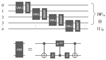
Figure 11: Circuit for generating the $|W\rangle$ state for arbitrary $n$. SWAP gates are added for illustration on 1D architecture of physical qubits. Qubit $n$ is discarded at the end.

C.2 Reverse engineering for $W$-state preparation

Wang, Ashhab, and Nori Wang et al. (2009) outline a procedure to produce arbitrary states with fixed particle number. The approach is a recursive approach and scales as $O(2^{m}n^{m}/m!)$ where $m$ is the number of spin up or $|1\rangle$ and $n$ is the number of qubits. For the $W$-state case, $m=1$, the number of CNOT gates scales as $O(2n)$.

A target state that we want to prepare is transformed to the $|0\rangle^{\otimes n}$ by using a series of generalized Hadamard gates and controlled generalized Hadamard gates. The generalized Hadamard has the form $\tilde{H}=C^{\dagger}XC$, where

$$C=\begin{pmatrix}u&-v^{*}\\ v&u^{*}\end{pmatrix}$$ (45)

is a unitary matrix. For any single-qubit state $\cos\theta|0\rangle+\sin\theta e^{i\phi}|1\rangle$, it is easy to determine a $\tilde{H}$ that takes it to $|0\rangle$:

$$\tilde{H}=\begin{pmatrix}u^{*}v+uv^{*}&(u^{*})^{2}-(v^{*})^{2}\\ u^{2}-v^{2}&-(u^{*}v+uv^{*})\end{pmatrix}\begin{pmatrix}\cos\theta\\ \sin\theta e^{i\phi}\\ \end{pmatrix}=\begin{pmatrix}1\\ 0\\ \end{pmatrix}$$ (46)

Consider the set of states in the computational basis that correspond to Hamming-weight-1 bit strings, $\{X_{i}{|0\rangle}^{\otimes n}\}_{i=1}^{n}$, $W$-state is a uniform superposition of these states

$$|W_{n}\rangle=\frac{1}{\sqrt{n}}\sum_{i=1}^{n}X_{i}{|0\rangle}^{\otimes n}\;,$$ (47)

where $n$ indicates the number of qubits. This wavefunction can be expressed as the first qubit and the rest $n-1$ qubits:

$$|W_{n}\rangle=c_{0}|0\rangle|W_{n-1}\rangle+c_{1}|1\rangle|0\rangle^{\otimes(n-1)}$$ (48)

where $c_{1}=1/\sqrt{n}$ and $c_{0}=\sqrt{(n-1)/n}$. Define an operator $Q_{n-1}$ that takes $|W_{n-1}\rangle$ to $|0\rangle^{\otimes(n-1)}$.

$$Q_{n-1}|W_{n-1}\rangle=|0\rangle^{\otimes(n-1)}$$ (49)

An $X$ operation on the first qubit in Eq. (48) followed by a controlled-$Q_{n-1}$ operation (the first qubit being the controlling qubit) creates the state $\big{(}c_{0}|0\rangle+c_{1}|1\rangle\big{)}{|0\rangle}^{(n-1)}$, to which we can perform the generalized Hadamard to evolve to the zero state $|0\rangle^{\otimes n}$. Analogously We can define $Q_{n-1}$ using controlled-$Q_{n-2}$ and so on until the base case for the recursion, $|W_{2}\rangle$, which is also the Bell state,

$$|\beta\rangle=a|10\rangle+b|01\rangle$$ (50)

which can be brought to $|00\rangle$ by an $X$ gate followed by a generalized Hadamard. Inverse the whole circuit above gives the circuit to prepare $W$-state from the ${|0\rangle}^{\otimes n}$ state.

Reference Wang et al. (2009) outlines a procedure to produce arbitrary states with fixed particle number through a recursive approach that scales as $O(2^{m}n^{m}/m!)$ where $m$ is the number of spin up or $|1\rangle$ and $n$ is the number of qubits. When considering creation of single-excitation states, or $W$-states, the circuits have $\mathcal{O}(n)$ CNOT gates single qubit gates with only nearest-neighbor physical coupling.

As an example for constructing an even superposition of three-excitations, a $W$-state, we provide the Quil Smith et al. (2016) and Cirq code below.

• Quil code for the W-state

  RY(acos(-1/3)) 2
  PHASE(-pi/2) 2
  RY(pi/4) 1
  CNOT 2 1
  RY(-pi/4) 1
  RZ(pi/2) 1
  CNOT 2 1
  RZ(pi/2) 1
  CNOT 1 0
  CNOT 2 1
  X 2
  

• Cirq code for the W-state

  qubits = cirq.LineQubit.range(3)
  w_state = cirq.Circuit().from_ops([
   cirq.Ry(numpy.arccos(-1/3)).on(qubits[2]),
   cirq.ZPowGate(exponent=-1/2).on(qubits[2]),
   cirq.Ry(pi/4).on(qubits[1]),
   cirq.CNOT(qubits[2], qubits[1]),
   cirq.Ry(-pi/4).on(qubits[1]),
   cirq.Rz(pi/2).on(qubits[1]),
   cirq.CNOT(qubits[2], qubits[1]),
   cirq.Rz(pi/2).on(qubits[1]),
   cirq.CNOT(qubits[1], qubits[0]),
   cirq.CNOT(qubits[2], qubits[1]),
   cirq.X.on(qubits[2])])
  

C.3 Prepare generalized W-State via projective measurements

This section is about preparing generalized W-states through projective measurements proposed in Ref. Childs et al. (2002)

Procedure outline

We start with the $n$-qubit state ${|0\rangle}^{\otimes n}$ and apply the biased Hadamard gate

$$H=\left({\begin{array}[]{cc}\sqrt{1-\frac{w}{n}}&\sqrt{\frac{w}{n}}\\ \sqrt{\frac{w}{n}}&-\sqrt{1-\frac{w}{n}}\\ \end{array}}\right)^{\otimes n}\;.$$ (53)

The biased Hadamard gate will drive the initial state to $|\psi\rangle=H|0\rangle^{\otimes n}=\big{(}\sqrt{1-p}|0\rangle+\sqrt{p}|1\rangle\big{)}^{\otimes n}$ with $p=w/n$. Consider $|\psi\rangle$ measured in the computational basis, since the probability of each qubit being in $|0\rangle$ is $p$, the probability of getting a state of Hamming weight $w$ is $\Pr(w)=C^{w}_{n}p^{w}(1-p)^{n-w}$, which as a function of $w$ has a minimum at $w=n/2$ with $\Pr(w=n/2)=\frac{n!}{2^{n}(n/2)!(n/2)!}\approx\sqrt{\frac{2}{n\pi}}$, where the $\approx$ refers to large $n$ limit . Therefore $\Pr(w)\gtrsim\sqrt{\frac{2}{n\pi}}$ for any $w$. Specifically, for our interest of $w=1$, we have $p=1/n$ and

$$\Pr(w=1)=(1-\frac{1}{n})^{n-1}=(1+\frac{1}{n-1})^{-(n-1)}\approx\frac{1}{e}\;,$$ (54)

which is a fairly high probability.

If we can conduct a projective measurement on the Hamming weight (instead of measuring $\sigma^{z}$ on each qubit), then instead of collapsing to a state in the computational basis, the system is projected to the subspace of Hamming weight $w$. Given Eq. (54), with only a few repetitions one is expected to get $w=1$, accompanying a generalized W-state.

Now we describe the circuit to perform the projective measurement on the Hamming weight illustrated in Ref.[Chuang and Modha, 2000]. By definition the Hamming weight is the number of 1’s of a state in the computational basis. Computing the Hamming weight can be done by introducing an auxiliary register $W$, and apply a “controlled-add-1” gate on it. The “add-1” is conditioned on the qubit being in state 1. Since the Hamming weight is at most $n$, $\log n$ qubits are sufficient to encode $W$. Upon measuring the auxiliary qubits, one gets a generalized W-state when the measured $W=1$. Now we consider how the controlled-add-one is implemented. First, we review a more general operation controlled-add-k for any constant $k$ presented in Ref.[Cleve and DiVincenzo, 1996]. The idea is to use a $n$-bit auxiliary register $C$ to record whether a carry will happen for next bit. Populating $C$ bit by bit. In a second loop, do the real addition.

Program Conditional_Add_k

• Notation
  X : n-bit register
  B : bit register (control)
  C : n-bit auxiliary register (initialized and finalized to 0)
  

• Pseudo Code

$${\tt\bf Conditional\_Add\_k:}$$

for $$i=1 n-1$$ up to (55)

$$\leavevmode\nobreak\ \leavevmode\nobreak\ \leavevmode\nobreak\ \leavevmode\nobreak\ C_{i}\leftarrow C_{i}\oplus\text{MAJ}(k_{i-1},X_{i-1},C_{i-1})$$ (56)

endfor

for $$i=n-1$$ down to 1 (57)

$$\leavevmode\nobreak\ \leavevmode\nobreak\ \leavevmode\nobreak\ \leavevmode\nobreak\ X_{i}\leftarrow X_{i}\oplus(k_{i}\land B)$$ (58)

$$\leavevmode\nobreak\ \leavevmode\nobreak\ \leavevmode\nobreak\ \leavevmode\nobreak\ X_{i}\leftarrow X_{i}\oplus(C_{i}\land B)$$ (59)

$$\leavevmode\nobreak\ \leavevmode\nobreak\ \leavevmode\nobreak\ \leavevmode\nobreak\ C_{i}\leftarrow C_{i}\oplus\text{MAJ}(k_{i-1},X_{i-1},C_{i-1})$$ (60)

endfor

$$X_{0}\leftarrow X_{0}\oplus k_{0}$$ (61)

where the “majority” gate MAJ takes value true when at least 2 out of the three bits are true:

$$\text{MAJ}(O,P,Q)=\begin{cases}P\land Q&\text{if $O=0$}\\ P\lor Q&\text{if $O=1$}\end{cases}$$ (62)

We now explain the above pseudo-code.
Line 56, assuming $B=1$, i.e., the addition will happen, determines whether a carry will happen for the next bit, and record in $C_{i}$. A Toffli (controlled-controlled-not) gate is applied to $C_{i}$, with the control condition being that at least two bits in $\{k_{i-1},X_{i-1},C_{i-1}\}$ take value one. Because $C$ is initialized to be all zeros, the control condition being true will set $C_{i}=1$.
Line 58 and Line 59 implements the real addition of $k_{i}$ and $C_{i}$ to $X_{i}$, controlled by $B$.
Line 60 is exactly the same as Line 56, hence resets $C$ to zero.
Line 61 adds $k_{0}$ to $X_{0}$.

Now we consider the special case $k=1$. We only need a single-bit register for $k$: $k_{0}=1$. Line (56) reduce to $C_{1}=C_{1}\oplus(X_{0}\lor C_{0})$ and $C_{i}=C_{i}\oplus(X_{i-1}\land C_{i-1})$ for $i>1$. Therefore the pseudo-code is

Pseudo-code:

$${\tt\bf Conditional\_Add\_1:}$$

for $$i=1 n-1$$ up to (63)

$$\leavevmode\nobreak\ \leavevmode\nobreak\ \leavevmode\nobreak\ \leavevmode\nobreak\ \tt{SET\_C}$$ (64)

endfor

for $$i=n-1$$ down to 1 (65)

$$\leavevmode\nobreak\ \leavevmode\nobreak\ \leavevmode\nobreak\ \leavevmode\nobreak\ X_{i}\leftarrow X_{i}\oplus(C_{i}\land B)$$ (66)

$$\leavevmode\nobreak\ \leavevmode\nobreak\ \leavevmode\nobreak\ \leavevmode\nobreak\ \tt{SET\_C}$$ (67)

endfor

$$X_{0}\leftarrow\bar{X}_{0}$$ (68)

with subrutine

$$\leavevmode\nobreak\ \leavevmode\nobreak\ \leavevmode\nobreak\ \leavevmode\nobreak\ \tt{SET\_C:}$$ (69)

if $$i==1$$ (70)

$$\leavevmode\nobreak\ \leavevmode\nobreak\ \leavevmode\nobreak\ \leavevmode\nobreak\ \leavevmode\nobreak\ \leavevmode\nobreak\ \leavevmode\nobreak\ \leavevmode\nobreak\ C_{i}\leftarrow C_{i}\oplus(X_{i-1}\lor C_{i-1})$$ (71)

else

$$\leavevmode\nobreak\ \leavevmode\nobreak\ \leavevmode\nobreak\ \leavevmode\nobreak\ \leavevmode\nobreak\ \leavevmode\nobreak\ \leavevmode\nobreak\ \leavevmode\nobreak\ C_{i}\leftarrow C_{i}\oplus(X_{i-1}\land C_{i-1})$$ (72)

endif (73)

Number of gates: The circuit for computing the Hamming weight would involve $n$ Controlled_add_1 gates on the Hamming weight register $W$, each controlled by one data qubit. Since $W$ is composed of $\log n$ bits, each Controlled_add_1 requires $5\log n$ Toffoli (or Toffoli-like) gates. The total circuit requires $5n\log n$ Toffoli gates. With the probability $1/e$ of getting $W=1$ in the measurement, it will take on average three repetition, hence the expected number of Toffoli gates is $\sim 15n\log n$, which translates into $\sim 90n\log n$ CNot gates.

Note that when measurement is expensive, it would be more efficient to hold the measurement on $W$ after performing the computation of $W$, apply the following target algorithm, and measure $W$ in the end. This will triple the run time of the whole algorithm.

C.4 Applying $XY$ Hamiltonian

The $XY$ Hamiltonian on a 1D chain or ring can be exactly implemented in gate-model. Applying the $XY$ Hamiltonian on a state $|0\rangle$ can generate certain superposition of states in the subspace $S$ expanded by states corresponding to Hamming-weight-1 bit strings, but exact W-state may not be generated this way. The Hamiltonian for a 1D $XY$ model with n.n. coupling reads

$$H_{XY} = \sum_{c=1}^{m}\sigma^{x}_{c}\sigma^{x}_{c+1}+\sigma^{y}_{c}\sigma^{y}_{c+1}$$ (74)

$$= \frac{1}{2}\sum_{c=1}^{m}\big{(}\sigma^{+}_{c}\sigma^{-}_{c+1}+\sigma^{-}_{c}\sigma^{+}_{c+1}\big{)}$$ (75)

where periodic boundary condition (PBC) $\sigma_{m+1}=\sigma_{1}$ is implied. We now examine how well the ring transfers the a classical Hammint-weight-1 state.

C.4.1 State transfer using a $XY$ chain with open boundary condition (OBC)

If we remove the constraint of PBC, i.e., work on a open-end chain instead of ring, it is known that perfect state transfer can be achieved along a $XY$ chain only for $n=2$ and $n=3$. The fidelity can be computed by diagonalizing the Hamiltonian, in this case the eigenvectors reads

$$|k\rangle=\sqrt{\frac{2}{m+1}}\sum_{n=1}^{m}\sin(\frac{nk\pi}{N+1})|n\rangle$$ (76)

and the eigenvalues are $E_{k}=2\cos(\frac{k\pi}{m+1})$. Furthermore, if inhomogeneous coupling between n.n. qubits along the chain is allowed, perfect transfer can be realized for any chain length.Christandl et al. (2004)

C.4.2 State transfer using a $XY$ chain with PBC

We now study how the state $|0\rangle$ is transferred along a ring. We apply Jordan-Wigner transformation Lieb et al. (1961); Barouch et al. (1970) to $H_{B,j}$.

$$a_{c} = S^{-}_{c}e^{i\phi_{c}}$$ (77)

$$a_{c}^{\dagger} = S^{+}_{c}e^{-i\phi_{c}}$$ (78)

where $S^{+}_{c}=(\sigma^{x}_{c}+i\sigma^{y}_{c})/2$, $S_{c}^{-}=(\sigma^{x}_{c}-i\sigma^{y}_{c})/2$, and the phase factor $\phi_{c}=\pi\sum_{c^{\prime}<j}(\sigma^{z}_{c^{\prime}}+1)/2$ is long-ranged involving all operators for $c^{\prime}<c$. The new operators $a_{c},\leavevmode\nobreak\ a_{c}^{\dagger}$ can be verified to obey the fermion anticommutation relations, $\{a_{c},a_{c^{\prime}}^{\dagger}\}=a_{c}a_{c^{\prime}}^{\dagger}+a_{c^{\prime}}^{\dagger}a_{c}=\delta_{c,c^{\prime}}$, and $\{a_{c},a_{c^{\prime}}\}=\{a_{c}^{\dagger},a_{c^{\prime}}^{\dagger}\}=0$. The inverse transformation reads

$$S_{c}^{+} = a_{c}^{\dagger}e^{i\phi_{c}}$$ (79)

$$S_{c}^{-} = a_{c}e^{-i\phi_{c}}$$ (80)

$$\sigma^{z}_{c} = 2a^{\dagger}_{c}a_{c}-1$$ (81)

and the phase factor in the fermionic representation is $\phi_{c}=\pi\sum_{c^{\prime}<c}a^{\dagger}_{c^{\prime}}a_{c^{\prime}}$. The Jordan-Wigner transformation is a convenient tool for one-dimentional spin systems, particularly for nearest-neighbored couplings because in product of the neighboring spin operators like $S_{c}^{+}S_{c+1}^{-}$, the phase factors drop out, leaving a concise expression with short-ranged coupling.

Apply the transformation to our problem, For simplicity, we omit the index $j$ in the Pauli operators for this section, and without loss of generality we use ${\cal P}_{j}=\{1,2,\ldots,m\}$ . We get

$$H_{XY} = 2\sum_{c=1}^{m-1}a_{c}^{\dagger}a_{c+1}-a^{\dagger}_{m}a_{1}G+h.c.$$ (82)

and the initial state $|1,0,\cdots,0\rangle$ in the fermionic representation becomes

$$|\Phi\rangle_{0}=a^{\dagger}_{1}|\bf 0\rangle$$ (83)

where $|\bf 0\rangle$ denotes the vacuum state. (the 0-eigenstate of the total particle number operator $\hat{N}_{\text{tot}}=\sum_{c}a^{\dagger}_{c}a_{c}$). Here we introduced gauge operator $G=\exp[i\pi\sum_{l=1}^{m}a^{\dagger}_{l}a_{l}]=\prod_{l=1}^{m}(-)\sigma^{z}_{l}$. The initial state has only one spin up, hence corresponds to $G=-1$. Because $G$ commutes with both $H_{B}$ and $H_{C}$, it is a constant of motion and its value statys $-1$ throughout the evolution. We can therefore replace $G$ with $-1$ in Eq. (82):

$$H_{XY} = 2\sum_{c=1}^{m}a_{c}^{\dagger}a_{c+1}+h.c.$$ (84)

This Hamiltonian can be diagonalized by introducing the Fourier transformation $f_{k}=\frac{1}{\sqrt{m}}\sum_{c=1}^{m}\exp[-ick\omega]a_{c}$, with $\omega=\frac{2\pi}{N}$. The diagonalized Hamiltonian is

$$H_{XY} = \sum_{k=1}^{m}E_{k}f_{k}^{\dagger}f_{k}$$

where the eigen-energies $E_{k}=2\cos(2k\pi/m)$ and the eigen states are

$$|\psi_{k}\rangle = f^{\dagger}_{k}|0\rangle=\frac{1}{\sqrt{m}}\sum_{c=1}^{m}e^{ick\omega}a^{\dagger}_{c}|0\rangle$$ (86)

We now measure the expectation value of the occupation operator $\hat{n}_{c}=a^{\dagger}_{c}a_{c}$ for each site $c$. The occupation operator $\hat{n}_{c}$ taking value 1 indicates the the spinless fermion particle is at site $c$, and correspondingly in the spin problem the spin on site $c$ is up.

At time $t$ the fidelity of sate transfer at site $c$ can be analytically derived to be

$${\cal F} \equiv \text{T}r[\hat{n}(c)e^{-itH_{XY}}|\Phi_{0}\rangle\langle\Phi_{0}|e^{itH_{XY}}]$$ (87)

$$= \Big{|}\frac{1}{m}\sum_{k}e^{i(c-1)k\omega}e^{-itE_{k}}\Big{|}^{2}$$ (88)

Figure. 12 shows for the problability evolution of the transfer fidelity at each site. For W-state generation, we are looking for a time when pupulation on all sites has equal probability, i.e., when curves of different color interacts at $1/n$. We see for $n$ up to 4, an exact W-state can be generated by choosing the right time $t$.

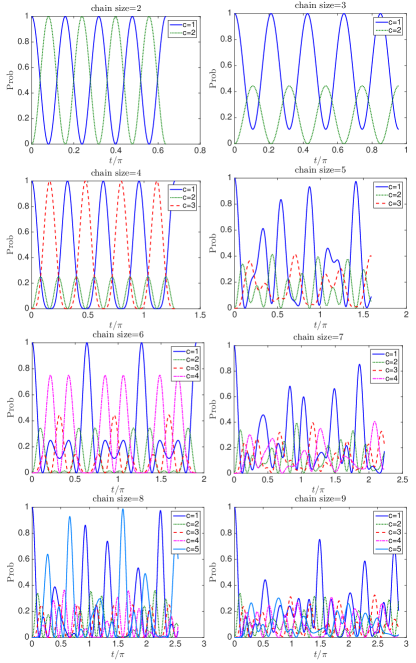
Figure 12: For ring size $m=2$ to 9, probability of spin-up at each site as a function of time $t$, under the evolution of the XY Hamiltonian on the ring.

References

- Farhi et al. (2014a) E. Farhi, J. Goldstone, and S. Gutmann, arXiv preprint arXiv:1411.4028 (2014a).
- Hadfield et al. (2017) S. Hadfield, Z. Wang, B. O’Gorman, E. G. Rieffel, D. Venturelli, and R. Biswas, arXiv preprint arXiv:1709.03489 (2017).
- Farhi et al. (2017) E. Farhi, J. Goldstone, S. Gutmann, and H. Neven, arXiv preprint arXiv:1703.06199 (2017).
- Jiang et al. (2017) Z. Jiang, E. G. Rieffel, and Z. Wang, Physical Review A 95, 062317 (2017).
- Wang et al. (2018) Z. Wang, S. Hadfield, Z. Jiang, and E. G. Rieffel, Physical Review A 97, 022304 (2018).
- Zhou et al. (2018) L. Zhou, S.-T. Wang, S. Choi, H. Pichler, and M. D. Lukin, arXiv preprint arXiv:1812.01041 (2018).
- Farhi et al. (2014b) E. Farhi, J. Goldstone, and S. Gutmann, arXiv preprint arXiv:1412.6062 (2014b).
- Shaydulin et al. (2018) R. Shaydulin, H. Ushijima-Mwesigwa, I. Safro, S. Mniszewski, and Y. Alexeev, arXiv preprint arXiv:1810.12484 (2018).
- Farhi and Neven (2018) E. Farhi and H. Neven, arXiv preprint arXiv:1802.06002 (2018).
- Otterbach et al. (2017) J. Otterbach, R. Manenti, N. Alidoust, A. Bestwick, M. Block, B. Bloom, S. Caldwell, N. Didier, E. S. Fried, S. Hong, et al., arXiv preprint arXiv:1712.05771 (2017).
- Farhi and Harrow (2016) E. Farhi and A. W. Harrow, arXiv:1602.07674 (2016).
- O’Malley et al. (2016) P. J. J. O’Malley, R. Babbush, I. D. Kivlichan, J. Romero, J. R. McClean, R. Barends, J. Kelly, P. Roushan, A. Tranter, N. Ding, B. Campbell, Y. Chen, Z. Chen, B. Chiaro, A. Dunsworth, A. G. Fowler, E. Jeffrey, E. Lucero, A. Megrant, J. Y. Mutus, M. Neeley, C. Neill, C. Quintana, D. Sank, A. Vainsencher, J. Wenner, T. C. White, P. V. Coveney, P. J. Love, H. Neven, A. Aspuru-Guzik, and J. M. Martinis, Phys. Rev. X 6, 031007 (2016).
- Fingerhuth et al. (2018) M. Fingerhuth, T. Babej, and T. Ing, arXiv preprint arXiv:1810.13411 (2018).
- Lechner (2018) W. Lechner, arXiv preprint arXiv:1802.01157 (2018).
- Guerreschi and Matsuura (2019) G. G. Guerreschi and A. Y. Matsuura, Scientific Reports 9, 6903 (2019), arXiv:1812.07589 [quant-ph] .
- Crooks (2018) G. E. Crooks, arXiv preprint arXiv:1811.08419 (2018).
- Venturelli et al. (2018) D. Venturelli, M. Do, E. Rieffel, and J. Frank, Quantum Science and Technology 3, 025004 (2018), arXiv:1705.08927 [quant-ph] .
- Booth et al. (2018) K. E. C. Booth, M. Do, J. C. Beck, E. Rieffel, D. Venturelli, and J. Frank, arXiv:1803.06775 (2018).
- Yang et al. (2017) Z.-C. Yang, A. Rahmani, A. Shabani, H. Neven, and C. Chamon, Phys. Rev. X 7, 021027 (2017).
- Hadfield (2018) S. Hadfield, arXiv preprint arXiv:1804.09130 (2018).
- McClean et al. (2016) J. R. McClean, J. Romero, R. Babbush, and A. Aspuru-Guzik, New Journal of Physics 18, 023023 (2016).
- Rubin et al. (2018) N. C. Rubin, R. Babbush, and J. McClean, New Journal of Physics 20, 053020 (2018).
- Robinson (1995) D. J. Robinson, A Course in the Theory of Groups, Graduate Texts in Mathematics, Vol. 80 (Springer, 1995).
- Jordan and Wigner (1928) P. Jordan and E. Wigner, Zeitschrift für Physik 47, 631 (1928).
- Babbush et al. (2017) R. Babbush, N. Wiebe, J. McClean, J. McClain, H. Neven, and G. K. Chan, arXiv preprint arXiv:1706.00023 (2017).
- Lieb et al. (1961) E. Lieb, T. Schultz, and D. Mattis, Annals of Physics 16, 407 (1961).
- Ferris (2014) A. J. Ferris, Phys. Rev. Lett. 113, 010401 (2014).
- Verstraete et al. (2009) F. Verstraete, J. I. Cirac, and J. I. Latorre, Phys. Rev. A 79, 032316 (2009).
- Kivlichan et al. (2018) I. D. Kivlichan, J. McClean, N. Wiebe, C. Gidney, A. Aspuru-Guzik, G. K.-L. Chan, and R. Babbush, Phys. Rev. Lett. 120, 110501 (2018).
- Jiang et al. (2018) Z. Jiang, K. J. Sung, K. Kechedzhi, V. N. Smelyanskiy, and S. Boixo, Phys. Rev. Applied 9, 044036 (2018).
- Lechner et al. (2015) W. Lechner, P. Hauke, and P. Zoller, Science Advances 1 (2015), 10.1126/sciadv.1500838, http://advances.sciencemag.org/content/1/9/e1500838.full.pdf .
- Rocchetto et al. (2016) A. Rocchetto, S. C. Benjamin, and Y. Li, Science Advances 2 (2016), 10.1126/sciadv.1601246, http://advances.sciencemag.org/content/2/10/e1601246.full.pdf .
- Kosowski and Manuszewski (2008) A. Kosowski and K. Manuszewski, in Contemporary Mathematics, Vol. 352 (2008) pp. 1–20.
- Schön et al. (2007) C. Schön, K. Hammerer, M. M. Wolf, J. I. Cirac, and E. Solano, Phys. Rev. A 75, 032311 (2007).
- Wang et al. (2009) H. Wang, S. Ashhab, and F. Nori, Physical Review A 79, 042335 (2009).
- Smith et al. (2016) R. S. Smith, M. J. Curtis, and W. J. Zeng, arXiv preprint arXiv:1608.03355 (2016).
- Childs et al. (2002) A. M. Childs, E. Farhi, J. Goldstone, and S. Gutmann, Quantum Info. Comput. 2, 181 (2002).
- Chuang and Modha (2000) I. L. Chuang and D. S. Modha, IEEE Transactions on Information Theory 46, 1104 (2000).
- Cleve and DiVincenzo (1996) R. Cleve and D. P. DiVincenzo, Phys. Rev. A 54, 2636 (1996).
- Christandl et al. (2004) M. Christandl, N. Datta, A. Ekert, and A. J. Landahl, Phys. Rev. Lett. 92, 187902 (2004).
- Barouch et al. (1970) E. Barouch, B. M. McCoy, and M. Dresden, Physical Review A 2, 1075 (1970).