Data Races and the Discrete Resource-time Tradeoff Problem with Resource Reuse over Paths
Abstract.
A determinacy race occurs if two or more logically parallel instructions access the same memory location and at least one of them tries to modify its content. Races are often undesirable as they can lead to nondeterministic and incorrect program behavior. A data race is a special case of a determinacy race which can be eliminated by associating a mutual-exclusion lock with the memory location in question or allowing atomic accesses to it. However, such solutions can reduce parallelism by serializing all accesses to that location. For associative and commutative updates to a memory cell, one can instead use a reducer, which allows parallel race-free updates at the expense of using some extra space. More extra space usually leads to more parallel updates, which in turn contributes to potentially lowering the overall execution time of the program.
We start by asking the following question. Given a fixed budget of extra space for mitigating the cost of races in a parallel program, which memory locations should be assigned reducers and how should the space be distributed among those reducers in order to minimize the overall running time? We argue that under reasonable conditions the races of a program can be captured by a directed acyclic graph (DAG), with nodes representing memory cells and arcs representing read-write dependencies between cells. We then formulate our original question as an optimization problem on this DAG. We concentrate on a variation of this problem where space reuse among reducers is allowed by routing every unit of extra space along a (possibly different) source to sink path of the DAG and using it in the construction of multiple (possibly zero) reducers along the path. We consider two different ways of constructing a reducer and the corresponding duration functions (i.e., reduction time as a function of space budget).
We generalize our race-avoiding space-time tradeoff problem to a discrete resource-time tradeoff problem with general non-increasing duration functions and resource reuse over paths of the given DAG.
For general DAGs, we show that even if the entire DAG is available to us offline the problem is strongly NP-hard under all three duration functions, and we give approximation algorithms for solving the corresponding optimization problems. We also prove hardness of approximation for the general resource-time tradeoff problem and give a pseudo-polynomial time algorithm for series-parallel DAGs.
Page Distribution
1. Introduction
A determinacy race (or a general race) (Netzer and Miller, 1992; Feng and Leiserson, 1999) occurs if two or more logically parallel instructions access the same memory location and at least one of them modifies its content. Races are often undesirable as they can lead to nondeterministic and incorrect program behavior. A data race is a special case of a determinacy race which can be eliminated by associating a mutual-exclusion lock with the memory location in question or allowing only atomic accesses to it. Such a solution, however, makes all accesses to that location serial and thus destroys all parallelism. Figure 1 shows an example.
Part I
![[Uncaptioned image]](/html/1904.09283/assets/pics/race.png)
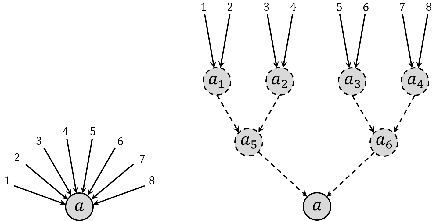
One can use a reducer (Frigo et al., 2009; Board, 1997; Reinders, 2007) to eliminate data races on a shared variable without destroying parallelism, provided the update operation is associative and commutative. Figure 3 shows the construction of a simple recursive binary reducer. For any integer such a reducer is a full binary tree of height and size with the shared variable at the root. Each nonroot node is associated with a unit of extra space initialized to zero. All updates to the shared variable are equally distributed among the leaves of the tree. Each node has a lock and a waiting queue to avoid races by serializing the updates it receives, but updates to different nodes can be applied in parallel. As soon as a node undergoes its last update, it updates its parent using its final value. In fact, such a reducer can be constructed using only units of extra space because if a node completes before its sibling it can become its own parent (with ties broken arbitrarily) and the sibling then updates the new parent. Assume that the time needed to apply an update significantly dominates the execution time of every other operation the reducer performs and each update takes one unit of time to apply. Then a reducer of height can correctly apply parallel updates on a shared variable in time provided at least processors are available. Hence, for large , the speedup achieved by a reducer (w.r.t. serially and directly updating the shared variable) is almost linear in the amount of extra space used.
To see how extra space can speed up real parallel programs consider the iterative matrix multiplication code Parallel-MM shown in Figure 3 which multiplies two matrices and and puts the results in another matrix ; that is, it sets for . Since every value can be computed independently of others, all iterations of the loops in Lines 1 and 2 can be executed in parallel without compromising correctness of the computation. However, the same is not true for the loop in Line 4 because if parallelized, for fixed values of and , all iterations of that loop will update the same memory location giving rise to data races and thus producing potentially incorrect results. Use of a mutual-exclusion lock or atomic updates for each will ensure correctness but in that case even with an unbounded number of processors, the code will take time to multiply the two matrices. Now if we put a reducer of height (integer ) at the top of each the time to fully update each and thus the overall running time of the code will drop to at the cost of using units of extra space. Observe that when , the running time of the code almost halves using units of extra space, and when , the running time drops to using extra space.
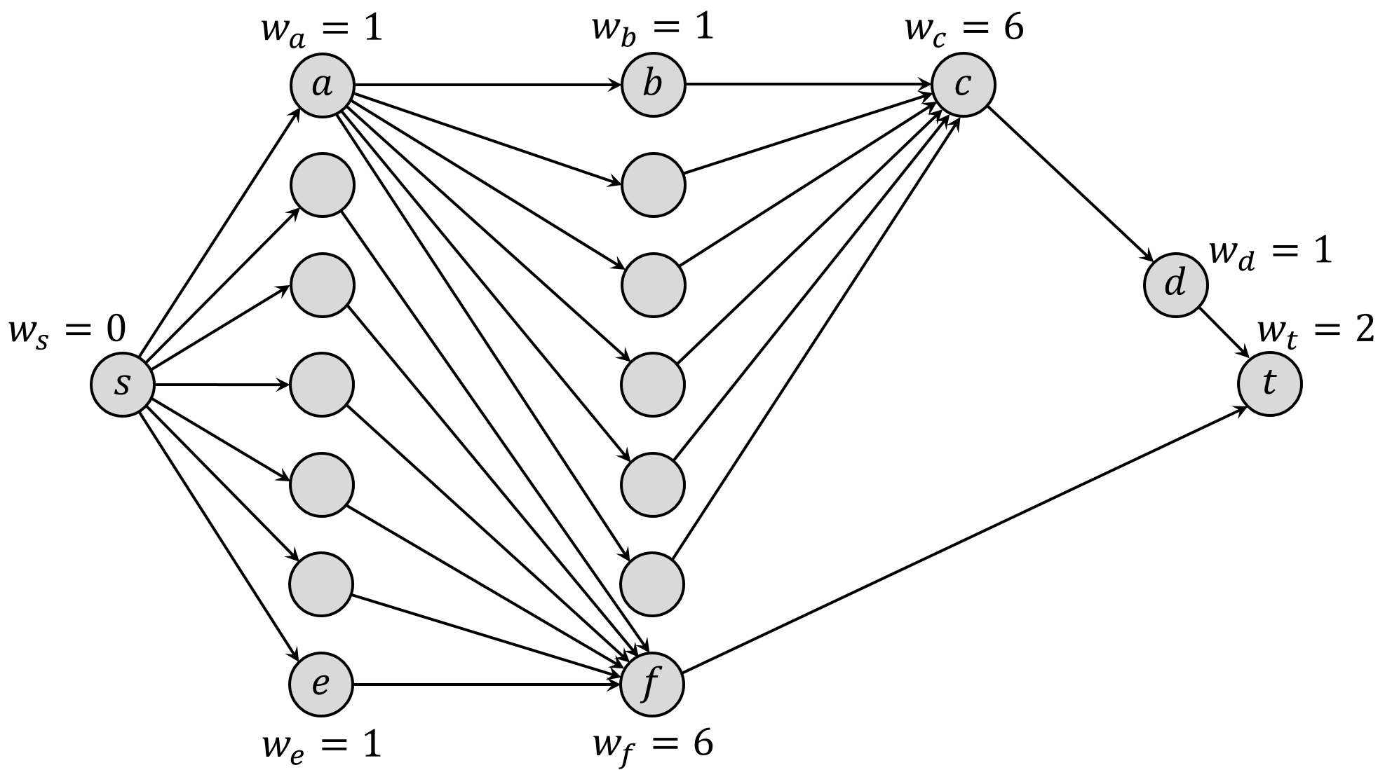
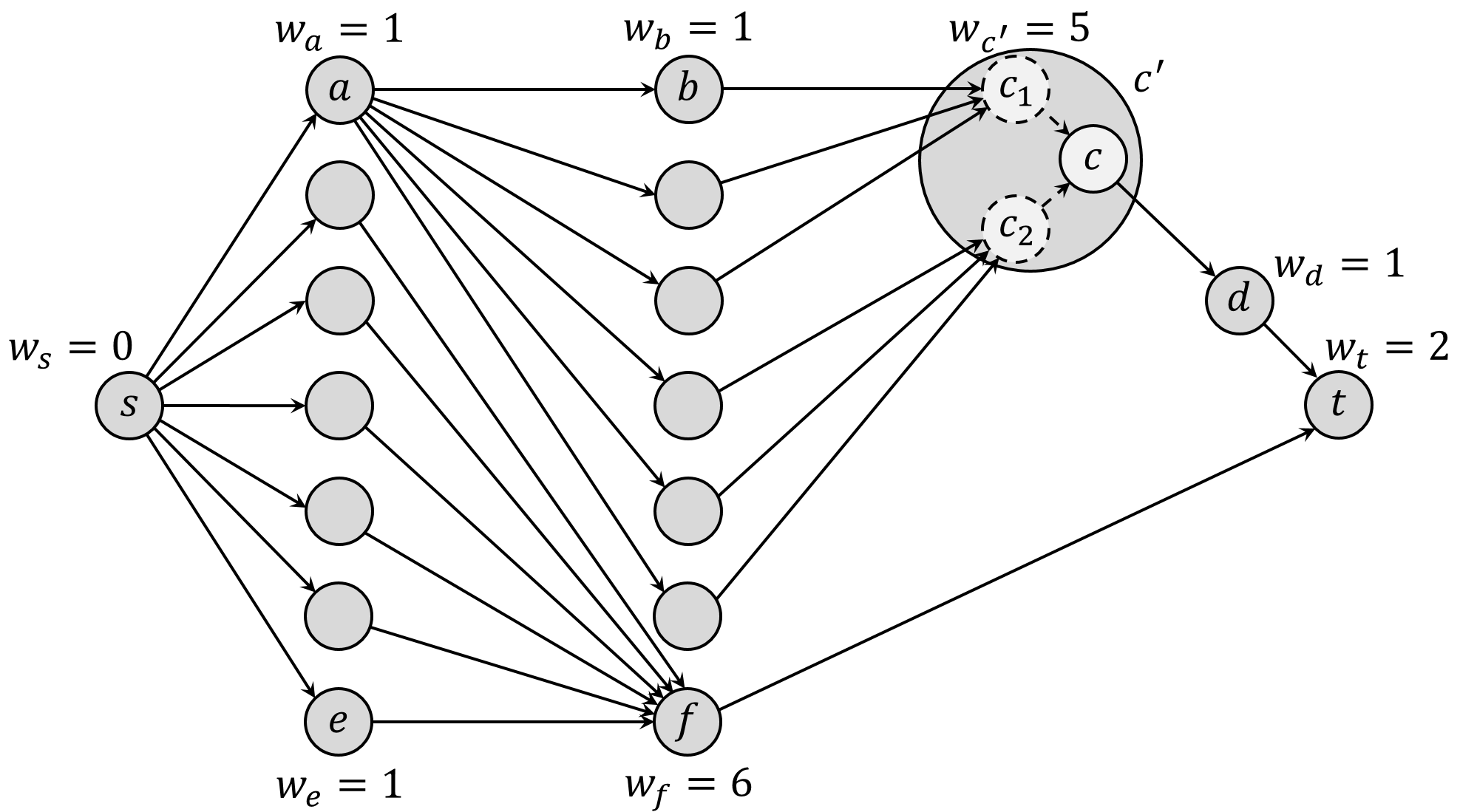
In order to analyze a program with data races, we capture those races in a directed acyclic graph (DAG) , assuming that there are no cyclic read-write dependencies among the memory locations accessed by . Figure 5 shows an example. We restrict to the set of programs that perform other operations between two successive writes to the memory, e.g., Parallel-MM in Figure 3. We assume that an update operation is significantly more expensive than any other single operation performed by and hence the costs of those operations can be safely ignored. Each node of represents a memory location, and a directed edge from node to node means that is updated using the value stored at . The in-degree of node gives the number of times is updated. With we also associate a work value and set . Assuming that each update operation requires unit time to execute and each node has a lock and a wait queue to serialize the updates, the value represents the time spent updating (excluding all idle times). The value also represents an upper bound on the time elapsed between the trigger time of any incoming edge of and the time the edge completes updating . We assume that updates along all outgoing edges of trigger as soon as all incoming edges complete updating . One can then make the following observation.
Observation 1.1.
The running time of with an unbounded number of processors is upper bounded by the makespan of 111To see why this is true start from the sink node and move backward toward the source by always moving to that predecessor of the current node that performed the last update on and noting that after edge was triggered it did not have to wait for more than time units to complete applying ’s update to ..
Then one natural question to ask is the following.
Question 1.1.
Given a fixed budget of units of extra space to mitigate the cost of data races in , which memory locations should be assigned reducers and how should the space be distributed among those reducers in order to minimize the makespan of ?
The question above ignores the possibility that space can be reused among reducers in . Indeed, after node reaches its final value (i.e., updated times) it can release all (if any) space it used for its reducer which can then be reused by some other node . A global memory manager can be used by the nodes to allocate/deallocate space for reducers. The following modified version of Question 1.1 now allows space reuse.
Question 1.2.
Repeat Question 1.1 but allow for space reuse among nodes of by putting all extra space under the control of a global memory manager that each node calls to allocate space for its reducer right before its first update and to deallocate that space right after its last update.
The problem with a single global memory manager is that it can easily become a performance bottleneck for highly parallel programs. Though better memory allocators have been developed for multi-core or multi-threaded systems (Aigner et al., 2015; Berger et al., 2000; lla, lloc; Schneider et al., 2006; TCM, ools), we can instead use an approach often used by recursive fork-join programs which avoids repeated calls to an external memory manager altogether along with the overhead of repeated memory allocations/deallocations. A single large segment of memory is allocated before the initial recursive call is made and a pointer to that segment is passed to the recursive call. Each recursive call splits and distributes its segment among its child recursive calls and reclaims the space when the children complete execution. So, we will assume that all the given extra space initially reside at the source node (i.e., node with in-degree zero). Then they flow along the edges toward the sink node (i.e., node with outdegree zero) possibly splitting along outgoing edges and merging at the tip of incoming edges as they flow. Each unit of space reaching node moves out of along some outgoing edge as soon as becomes fully updated and those edges trigger. Every unit of space may participate in the construction of multiple reducers (possibly zero) along the path it takes.
Question 1.3.
Repeat Question 1.1 but now allow for space reuse among nodes of by flowing each unit of space along a source to sink path and using it in the construction of zero or more reducers along that path.
While several existing results (De et al., 1997; Du and Leung, 1989; Skutella, 1998; Jansen and Zhang, 2006) can be extended to answer Questions 1.1 and 1.2, to the best of our knowledge, Question 1.3 had not been raised before. In this paper we investigate answers to Question 1.3 by extending it to a more general resource-time tradeoff question posed on a DAG in which nodes represent jobs (not necessarily of updating memory locations), resources (not necessarily space) flow along source to sink paths, and an general duration function (i.e., time needed to complete a job as a function of the amount of resources used) is specified for each node. We consider the following three duration functions: general non-increasing function for the general resource-time question, and recursive binary reduction and multiway (-way) splitting for the space-time case.
For general DAGs, we show that even if the entire DAG is available to us offline the problem is strongly NP-hard under all three duration functions, and we give approximation algorithms for solving the corresponding optimization problems. We also prove hardness of approximation for the general resource-time tradeoff problem and give a pseudo-polynomial time algorithm for series-parallel DAGs. Our main results are summarized in Table 1.
Related Work
While several prior works either directly or indirectly address Questions 1.1 (nonreusable resources) and 1.2 (globally reusable resources), to the best of our knowledge, Question 1.3 (reusable along flow paths) has not been considered before.
The well-known time-cost tradeoff problem (TCTP) is closely related to our nonreusable resources question. In TCTP, some activities are expediated at additional cost so that the makespan can be shortened. Deadline and budget problems are two TCTP variants with different objectives. While the deadline problem seeks to minimize the total cost to satisfy a given deadline, the budget problem aims to minimize the project duration to meet the given budget constraint (Akkan et al., 2005). Most researchers consider the tradeoff functions to be either linear continuous or discrete giving rise to linear TCTP and discrete TCTP, respectively.
Linear TCTP was formulated by Kelley and Walker in 1959 (Kelley Jr and Walker, 1959). They assumed affine linear and decreasing tradeoff functions. In 1961, linear TCTP was solved in polynomial time using network flow approaches independently by Fulkerson (Fulkerson, 1961) and Kelley (Kelley Jr, 1961). Phillips and Dessouky (Phillips Jr and Dessouky, 1977) later improved that result.
In 1997, De et al. (De et al., 1997) proved that discrete TCTP is NP-hard. For this problem, Skutella (Skutella, 1998) proposed the first approximation algorithm under budget constraints which achieves an approximation ratio of , where is the ratio of the maximum duration of any activity to the minimum one. Discrete TCTP can also be used to approximate the TCTP with general time-cost tradeoff functions, see, e.g., Panagiotakopoulos (Panagiotakopoulos, 1977) and Robinson (Robinson, 1975). For details on discrete TCTP see De et al. (De et al., 1995).
Our problem with globally reusable resources (Question 1.2) is very similar to the problem of scheduling precedence-constrained malleable tasks (Turek et al., 1992). In 1978, Lenstra and Rinnooy Kan (Lenstra and Rinnooy Kan, 1978) showed that no polynomial time algorithm exists with approximation ratio less than unless . About 20 years later, Du and Leung (Du and Leung, 1989) showed that the problem is strongly NP-hard even for two units of resources. In 2002, under the monotonous penalty assumptions of Blayo et al (Blayo et al., 1999), Lepère et al. (Lepère et al., 2002) first proposed the idea of two-step algorithms – computing an allocation first, and then scheduling tasks, and used this idea (Lepere et al., 2002) to design a algorithm that achieve an approximation ratio of . In the first phase, they approximate an allocation using Skutella’s algorithm (Skutella, 1998). Similarly, based on Skutella’s approximation algorithm, Jansen and Zhang (Jansen and Zhang, 2006) devised a two-phase approximation algorithm with the best-known ratio of and showed that the ratio is tight when the problem size is large. For more details on the problems of scheduling malleable tasks with precedence constraints, please check Dutot et al. (Dutot et al., 2004).
There are memory allocators based on global memory manager for multi-core or multi-threaded systems such as scalloc (Aigner et al., 2015), Hoard (Berger et al., 2000), llalloc (lla, lloc), Streamflow (Schneider et al., 2006), and TCMalloc (TCM, ools). They use thread-local space for memory allocation and a global manager for memory deallocation/reuse. For the global manager, they use concurrent data structures. However, these data structures can not completely avoid the need for synchronization (Aigner et al., 2015; Henzinger et al., 2013; Shavit, 2011) without compromising correctness.
2. Preliminaries, Problem Formulation
In general, the option to use reducers to trade off between extra space and the time to complete race-free writing operations leads to a discrete resource-time tradeoff problem, where, here, the valuable “resource” is the space that is added, in order to reduce the time necessary for the write operations. By investing in additional space, we can reduce the time it takes to do conflict-free write operations.
We formalize the discrete resource-time tradeoff problem. Consider a DAG, , whose vertices correspond to jobs, and whose edges represent precedence relations among jobs. Without loss of generality, we assume that the DAG has a single source and a single sink vertex. The duration of a job depends on how much resource it receives. For each job , there is a non-increasing duration function that denotes the time required to complete job using units of resources. We call a resource-time tuple associated with job (vertex) . We consider three classes of duration functions – general non-increasing step functions, -way splitting functions, and recursive binary splitting functions.
General non-increasing step function. Let be the number of resource-time tuples associated with job . The -th resource-time tuple is where . Then, the duration function is a step function with steps described as follows:
| (1) |
where and for .
-way splitting. A -way split reducer utilizes units of extra space, , associated with a vertex , with , such that the write operations associated with incoming edges at are distributed among the vertices , which then have edges linking each to . The duration function that results from -way split reducers is given by
| (2) |
Recursive binary splitting. The duration function that results from a recursive binary split reducer is given by a step function, as follows. The resource-time tuples are defined for and where and . The duration function is minimized when (by differentiating w.r.t. ).
| (3) |
When utilizing a reducer, extra space serves as the limited resource and the time taken for race-free writing at a vertex is the duration of the job corresponding to . Both the -way splitting duration function and the recursive binary splitting duration function are special cases of general non-increasing function.
We consider jobs whose duration functions are of the types described above, and we distinguish between two optimization problems, depending on the objective function:
Minimum-Makespan Problem. Given a resource budget of , assign the resources to the vertices such that the makespan of the project is minimized. Resources can be reused over a path.
Minimum-Resource Problem. Given a makespan target of , minimize the amount of resources to achieve target makespan. Resources can be reused over a path.
Finally, we remark that instead of jobs corresponding to vertices of the DAG, we can transform the DAG into another DAG in which jobs correspond to edges of , and the precedence relations among jobs are enforced by introducing dummy edges, as follows: For each node in , we introduce an edge in (which then has the corresponding duration function, specified, e.g., by resource-time tuples). For each edge of , we introduce a dummy edge, in , from the endpoint of edge to the origin of edge , with resource-time function for all valid resource levels .
3. Approximation Algorithms
3.1. Bi-criteria Approximation for Non-increasing Duration Functions
We use linear programming in our approximation algorithms. First, we relax the discrete duration function to a linear one. We transform the DAG so that a relaxed linear non-increasing duration function can be used. The transformation happens in two steps.
Activity on arc reduction. We reduce the input DAG into an equivalent DAG with activities on arcs instead of nodes. This is a simple transformation described earlier in Section 2.
.
.
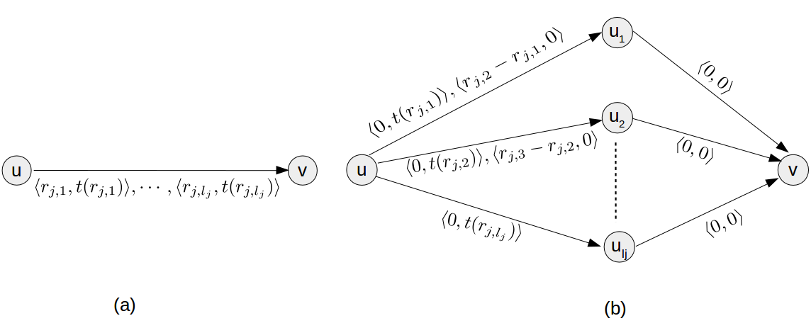
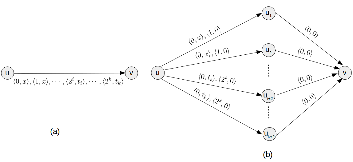
Activity with two tuples. Following (Skutella, 1998), we create a DAG from such that all activities in are still on arcs and each such activity has at most resource-time tuples as shown in Figure 7(b). Let be a job with resource-time tuples with and (following Equation 1). Let edge of represent job . We add parallel chains, each consisting of two edges in (Figure 7). For , we create a chain of two edges and . We create a job for arc and associate two resource-time tuples with it. For , job can be finished either using resource in units of time or using units of resource in unit of time. The logic is that job ’s duration can be reduced from to provided the resource difference is allocated to . Thus the duration function is and . Job ’s (bottom most edge in the parallel edges for job ) duration cannot be further improved from units of time by using extra resources. The resource-time tuple at edge is where .
There is a canonical mapping of resource usages and durations for jobs to that of job . Let be the units of resource used for job , then for job , units of resource are used. The time taken to finish job is . Without loss of generality, if we use unit of resource for job if , then this mapping is bijective. Thus we get the following lemma.
Lemma 3.1.
Any approximation algorithm on DAG (activity on edge and each edge has at most two resource-time tuples) with an approximation ratio implies an approximation algorithm with the same approximation ratio on general DAG (activity on vertex and each job can have more than two resource-time tuples).
From now on, we will only consider DAGs whose edges represent jobs, with each edge having at most two resource-time tuples.
Linear relaxation. In , any edge can have either two resource-time tuples or a single resource-time tuple . With linear relaxation, units of resource can be used to reduce the completion time of the job corresponding to edge that has two resource-time tuples. The corresponding duration function is as follows:
| (4) |
The linear duration function for the job with single resource-time tuple is as follows:
| (5) |
Linear programming formulation. Since we are allowed to reuse resources over a path we can model the problem as a network flow problem where resources are allowed to flow from the source to the sink in the DAG . Let be the set of edges in . Let denote the amount of resources that flow through the edge . Using linear relaxation on edge , the time taken to finish the activity is . Let the vertices in denote events. From now onwards, we use a vertex and its corresponding event synonymously. Let be the set of edges that are incident on vertex . Event occurs if and only if all the jobs corresponding to the edges in set are finished. Let denote the time when event occurs. Let and denote the source vertex and the sink vertex, respectively. For source vertex , we assume . All variables are non-negative.
Constraints:
| (6) |
| (7) |
| (8) |
| (9) |
Objective function:
| (10) |
Inequality 6 upper bounds the resource flow variable for edges with two tuples. This ensures that these variables remain in the range and the duration function is linear in this range. Note that there is no such upper bound on the edges with single resource-time tuple (except the trivial total resource budget upper bound). This allows the flow of more resources over an edge that can be used later on a path. Equation 8 is a flow conservation constraint for all the vertices . Inequality 9 constrains the flow of resources from source to be upper bounded by the resource budget.
Solving the LP and rounding. We first solve the LP described above. This might give solution as fractional flow and duration at edge . Let the resource-time tuples at edge be . The range of feasible duration of activity is . We divide this range into two parts where . If we round it down to , otherwise, we round it up to . Observe that in the first case, the resource requirement at can be increased by at most a factor of . In the second case, the completion time can be increased at most by a factor of . Let denote the rounded integer resource requirement at edge .
Computing min-flow. After rounding the LP solution, we get an integral resource requirement for every edge . We now compute a min-flow through this DAG where serves as the lower bound on the flow through (or resource requirement at) edge .
Constraints:
| (11) |
| (12) |
Objective function:
| (13) |
Proof.
Lemma 3.3.
is an integral flow and , where .
Proof.
Bi-criteria approximation. We now summarize our bi-criteria approximation result for general non-increasing duration functions:
Theorem 3.4.
For any , there is a bi-criteria approximation algorithm for the discrete resource-time tradeoff problem with an general non-increasing duration function which allows resource reuse over paths.
Proof.
First, we know from lemma 3.3 that is an integral flow and , where .
Second, we claim that the makespan of the DAG used in the minflow LP 11–13 is at most a factor of away from that of the LP 6–10 solution. Let us consider any path . The makespan is at least the sum of completion times of the edges in . Now, after rounding the LP 6–10 solution, the completion time of an edge may increase at most by a factor of . Hence, the sum of duration of edges along any path is increased at most by a factor of , thus the makespan will be increased by at most a factor of . ∎
3.2. Single-criteria Approximation for -Way and Recursive Binary Splitting
First, observe the prior section gives us a bi-criterian approximation for both -way and recursive binary splitting. Setting in Theorem 3.4, we obtain a bi-criteria approximation. Now, after LP rounding, say a job uses units of resource and takes units of time. Then the optimal solution uses units of resource and takes units of time for job . Recall that job consists of parallel jobs where . Hence, is the sum of the resource (after rounding) used by parallel jobs and is the maximum time (after rounding) taken by parallel jobs.
Approximation algorithm for -way splitting. To obtain a single-criteria approximation, in the case of -way splitting, we use at most units of resource for job . If , we reduce to (a nonnegative integer) units of resource such that . Using units of resource, job takes units of time to complete.
Lemma 3.5.
for where and .
Proof.
Since for , we have . Also since and for , we have . Hence, . ∎
Lemma 3.6.
If then .
Proof.
We know as . Also in lemma 3.5, we prove . However, we show that . Hence, combining these two results we get . ∎
Lemma 3.7.
If then .
Proof.
Recall that in , job is represented as parallel jobs where . The resource-time tuples of jobs and are and , respectively. To attain duration, requires at least units of resource and job requires unit of resource (applying linear relaxation). Hence, units of resource to achieve . ∎
Lemma 3.8.
If then .
Proof.
If and , then we round down to . So, from Lemma 3.7 it follows that after rounding down to unit of resource, job takes units of time.
If and , then we round to . It is true that because . Also, . Combining this two results we get . ∎
So, now we have the following result.
Theorem 3.9.
There is a -approximation algorithm for the minimum-makespan problem with -way splitting duration function.
Proof.
Combining Lemmas 3.8 and 3.6 we get for all valid . This proves that the makespan is at most 5 times the optimal solution. We now calculate the total amount of resource required to flow from the source of . We compute a min-flow in where is the resource requirement for job . Note that we are now working on that does not have parallel chains for job . Let be the min flow from the source of such that all the resource requirements are met. The flow from the LP solution before rounding is also a valid flow for the resource requirement for job as . We know that min-flow gives an optimal integral solution. Hence, . ∎
Approximation algorithm for recursive binary splitting. We have the following result.
Theorem 3.10.
There is a -approximation algorithm for the minimum-makespan problem with recursive binary splitting function.
Proof.
As in the case of k-way splitter, to get a single-criteria approximation, we use no more than units of resource for job . If , we reduce to . We know that from the properties of the recursive binary splitting function. Thus, . ∎
3.3. Improved Bi-criteria Approximation for Recursive Binary Splitting Functions
Putting in Theorem 3.4 we obtain a bi-criteria approximation algorithm for general non-increasing duration functions. Hence, if we use times more resources than OPT (i.e., the optimal solution), we are guaranteed to get a makespan within factor of 4 of OPT. In this section we show that the bound can be improved to for recursive binary splitting functions.
For a node with in-degree , the resource-time tuples based on the recursive binary splitting function are as follows: where for and is the largest value of for which decreases with the increase of . See Figure 7.
After solving LP 6–10 from Section 3.1, we sum up the (possibly fractional) resources allocated to all the parallel edges corresponding to job . Let be that sum. Let be the maximum among the time values given by the LP solution for the parallel edges. Thus, the LP takes units of time for job .
We round to an integer based on the following criteria.
We want to find a constant , such that if , then the LP must use at least units of resources. We compute as follows. In Figure 7, each of the top two edges and requires units of resource to finish in time . Each edge for requires units of resource to finish in time . Summing over all these edges, we get the expression of
Since we want to have , we want to find the smallest value of such that
Now,
Let, , and .
Note that , since . Hence,
Now, and hence,
Thus, .
Therefore, .
So, by setting , we get .
Summarizing, we get the following lemmas from the computation above.
Lemma 3.11.
To achieve a duration of for any job , the LP solution uses at least units of resources for .
Lemma 3.11 implies the following.
Lemma 3.12.
If the LP uses units of resources and we round down to where , then where is the duration from the LP solution.
Lemma 3.13.
With units of resource, the LP cannot achieve a duration of for job .
Proof.
The first edge has resource-time tuples . To achieve a duration of , the LP has to use unit of resource on the first edge. The second edge also has the same resource-time tuples , and it also takes unit of resource. Thus, the first two edges alone need unit of resource to achieve a duration of for all parallel edges of job . ∎
Lemma 3.13 implies the following.
Lemma 3.14.
If the LP uses unit of resource and we round down to , then , where is the duration from the LP solution.
Lemma 3.15.
If rounded to then
Proof.
When we use units of resource after rounding, the LP uses at least units. Thus, . ∎
Theorem 3.16.
There is a bi-criteria approximation algorithm for the discrete resource-time tradeoff problem with resource reuse along paths when the recursive binary duration function is used.
3.4. Exact Algorithm for Series-Parallel Graphs
We consider now the special case in which the underlying DAG is a series-parallel graph. A series-parallel graph can be transformed into (and represented as) a rooted binary tree in polynomial time by decomposing it into its atomic parts according to its series and parallel compositions (see, e.g., (Möhring, 1989)). In , the leaves correspond to the vertices of . Internal nodes of are labeled as “” or “” based on series or parallel composition. We associate each internal node of with the series-parallel graph , induced by the leaves of the subtree rooted at .
Let denote the makespan of using units of resources where is the resource budget. We want to solve for , where is the root of . This can be done using dynamic programming, solving for the leaves first, and then progressing upward to the root of . We compute as follows which assumes that node corresponds to job if it is a leaf, otherwise it has two children and .
There are nodes in if has edges. For each node we compute for . Computing for any particular value of takes time, since, if the node is a “” node, then for we need to look up values . Thus, for any internal node , it takes time. As there are nodes in , the (pseudo-polynomial) time complexity of the algorithm is .
4. NP-Hardness
In this section we give a variety of NP-hardness and inapproximability results related to the discrete time-resource tradeoff problem in the offline setting (i.e., when the entire DAG is available offline). All problems consider the version where there is resource reuse over paths, but they vary the cost-function, graph structure, and minimization goal. Section 4.1 gives several reductions from 1-in-3SAT. Theorem 4.1 gives a base reduction for the problem with general non-increasing duration function which will provide the ideas and structure for later more complex proofs. Theorems 4.3 and 4.4 adapt this proof to give constant factor inapproximability for the minimum-resource and minimum-makespan problems. Section 4.2 adapts the NP-hardness proof to apply when the cost function is restricted to be the recursive binary splitting and the -way splitting.
Section 4.3 considers the problem in bounded treewidth graphs. We show weak NP-hardness by a reduction from Partition.
 |
 |
4.1. Reuse Over a Path with General Non-increasing Duration Function
Theorem 4.1.
It is (strongly) NP-hard to decide if there exists a solution to the (offline) discrete resource-time tradeoff problem, with resource reuse over paths and a non-increasing duration function, satisfying a resource bound and a makespan bound .
Our proof is based on a polynomial-time reduction from the strongly NP-hard problem 1-in-3SAT (Schaefer, 1978): Given variables () and clauses (),with each clause a disjunction of three literals, is there a truth assignment to the variables such that each clause has exactly one true literal?
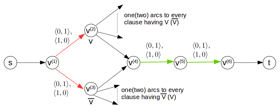
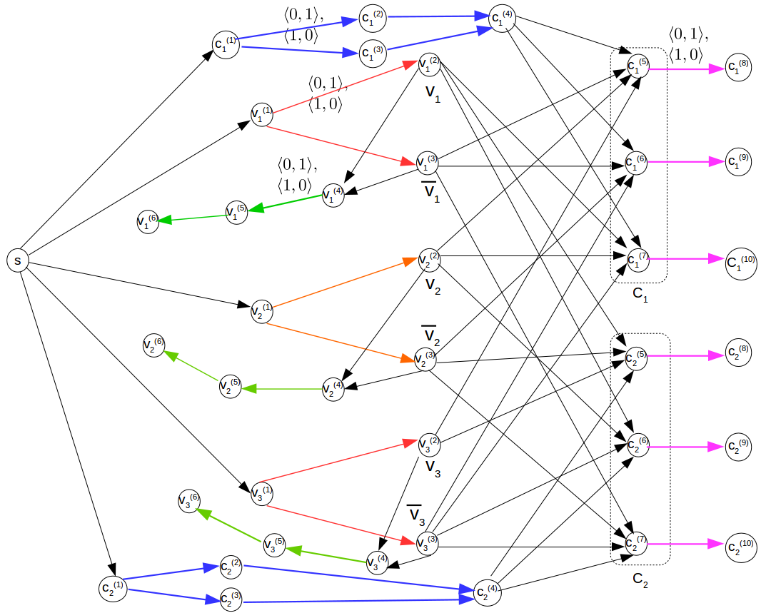
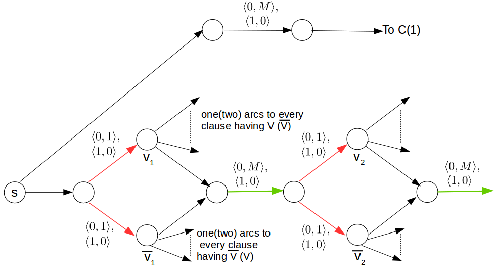
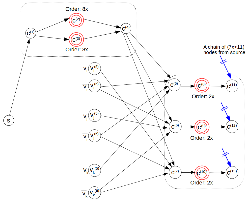
Variable gadget. The gadget for variable consists of nodes , , , , , and as shown in Figure 9. We show in the hardness proof that a variable gadget will get exactly one unit of extra resource, otherwise the makespan will be greater than the target makespan of . Sending one unit of resource to node (Figure 9) corresponds to setting the variable to TRUE and sending the unit of resource to corresponds to setting to FALSE. The remaining vertices ensure the extra resource is used in the variable and not transferred into one of the clauses.
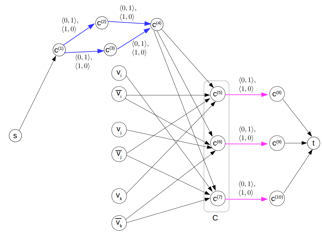
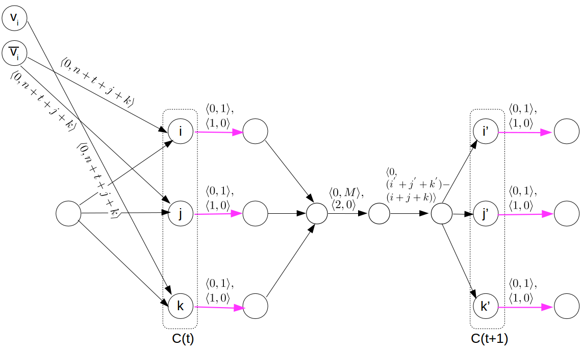
Clause gadget. The gadget corresponding to clause has vertices () as shown in Figure 9. Arcs , , and have resource-time pairs as . If clause has three literals and , then vertex is connected to the vertices and . These vertices correspond to and respectively. Vertex is connected to and . These vertices correspond to and . Vertex is connected to and . These vertices correspond to and . Arcs , , and have resource-time pairs as . The part of the clause gadget consisting of and demand at least two units of memory be allocated there and then these units of resource go to satisfy two of and . There is still one of these lines that has no allocated resource so it’s cost is 1. Thus the corresponding variable must have had it’s path length reduced (by setting it true).
Figure 9 shows the complete construction of as an example.
Lemma 4.2.
There exists a solution to the input instance of 1-in-3SAT iff there exists a valid flow of resources through the DAG achieving a makespan of under a resource bound of .
Proof.
Forward direction. We prove that if there is a solution to the 1-in-3SAT instance with variables and clauses, then the reduced DAG has a solution of makespan with units of resource. If a variable ’s truth assignment is TRUE, then we allow one unit of resource to flow through vertex along the path , otherwise we allow one unit of resource to flow through vertex along the path . For every clause , we allow one unit of resource to flow through the path and another unit of resource through the path . Thus, units of resource can be flowed from vertex . In a valid assignment of 1-in-3SAT, for each clause , exactly vertices of and will have the earliest start time of and the other one will have (Table 2).
Also, if only one literal is true in a clause, exactly two vertices among and need one unit of extra resource each to meet the makespan requirement (from Table 2). We are allowed to flow units of resource from vertex . Thus the project makespan is using units of resource.
Backward direction. Now, we prove that if there exists a solution of makespan using units of resource in the reduced DAG, then there also exists a solution to the 1-in-3SAT instance. To achieve a makespan of , every variable gadget needs unit of resource and each clause gadget needs units of resource, otherwise the makespan would be greater than . Also, any resource that is used in a variable gadget cannot be used further in any other variable or clause gadget because the resource can be reused over a path only. Similarly, any resource that is used in any clause gadget, cannot be reused in any other gadget. Only one vertex that is either or , will have the earliest start time . Both cannot be , as there is only unit of resource per variable gadget. Both cannot be as in a clause where the literal or is present, each of and would have earliest starting time of . This requires use of units of resource in the clause gadget to achieve a makespan of . However, each clause gadget can have exactly units of resource. Thus, for every variable, it has to be a valid assignment ( is set to either TRUE or FALSE). From Table 2, if a clause has exactly one TRUE literal, then the clause gadget requires units of resource to achieve a makespan of . Otherwise, the clause gadget would have a makespan of with the same amount of resource or would require more resource to achieve the target makespan of . Thus, each clause has exactly one TRUE literal. This satisfies the 1-in-3SAT instance. ∎
We also prove hardness of approximation, both for the minimum-makespan problem and for the minimum-resource problem. We begin with the minimum-makespan problem.
Theorem 4.3.
The minimum-makespan discrete resource-time tradeoff problem that allows resources to be reused only over paths cannot have a polynomial-time approximation algorithm with approximation factor less than unless .
Proof.
We prove the theorem by contradiction. Let’s assume that there is a polynomial time approximation algorithm with factor less than . Given a formula with variables and clauses, we construct the reduced DAG as described in the proof of Lemma 4.2. If the formula is a valid 1-in-3SAT instance, then OPT (i.e., the optimal solution) has a makespan of using units of resource in the reduced DAG. The approximation algorithm will return a schedule with makespan less than using units of resource. If the formula is not a valid 1-in-3SAT instance, then OPT’s makespan is greater than or equal to . So, the approximation algorithm will have a schedule with makespan greater than or equal to . Thus, using a polynomial time algorithm one can solve a strongly NP-hard problem. This is a contradiction. Hence, there exists no polynomial time approximation algorithm for resource-time-reuse-path problem with factor less than unless . ∎
Now, we turn attention to the minimum-resource problem:
Theorem 4.4.
The minimum-resource discrete resource-time tradeoff problem that allows resources to be reused only over paths cannot have a polynomial-time approximation algorithm with approximation factor less than unless .
Proof.
(Sketch) The proof uses a reduction from 1-in-3SAT; the construction is similar to that in the proof of Theorem 4.1, but has several key differences that make it considerably more intricate.
First, for each variable we have a gadget similar to before (Figure 9), with the option to send one unit of resource on one of two two-edge paths via a vertex, with the choice of which path indicating whether the variable is set to true or to false. Unlike the previous construction, we chain the variable gadgets together into a path of gadgets, from a source to a sink . Refer to Figure 11. A single unit of resource will be moved along the path, using one of each pair of two-edge paths, according to the truth assignments of the variables. A single directed edge, with options and , links variable gadget to variable gadget. Node is connected to the variable gadget with an edge with . A property of this construction is that the entry node of the gadget is reached by the unit of resource at exactly time , and the exit node of this gadget is reached at time exactly . At time the one unit of resource that traverses the path of variable gadgets emerges at time . Finally, there is also an edge directly from to with options and . In total, two units of resource will be moved through this part of the DAG: one will follow a path through the variable gadgets, according to the truth assignments of the variables, and the other will go directly along the edge . Both units of resource will arrive at at time .
The clause gadget consists of three vertices, each representing a literal. Each clause has an entry vertex and an exit vertex, and they are chained into a path of gadgets, with clauses ordered in a specific way, as described below. Refer to Figure 11. The exit vertex of one clause has an edge connecting it to the next clause in the order; these edges have specially chosen duration values in order to serve as “buffers”, as described below. The variable portion of the DAG feeds into the path of clause gadgets, with the 2 units of resource that arrive at at time moving along an edge that feeds into the first of the sequence of clause gadgets. Each of the three vertices of a clause gadget corresponds to a literal; each has an input edge coming from one of the two vertices of the variable gadget corresponding to the literal, according to whether the variable appears positively or negatively in the clause. These incoming edges have durations that are carefully chosen, so that the timing is as follows: For a clause with variables , , and , the two units of resource (which came through the variable portion of the DAG before entering the path of clause gadgets) will arrive at the entry to the clause at exactly time . The incoming edges from variables to the clause literals have durations chosen just so that the precedence constraints are satisfied “just in time”, for the two units of resource to pass through the clause gadget literals that are not true (using edges with duration 0, based on the resource of 1), while the one true literal vertex (who was reached within the clause gadget via an edge of duration 1, instead of 0, since there was no resource associated with it) is reached 1 unit of time sooner (from the variable gadget), to compensate. The net result is that both units of resource emerge out of a clause at time , ready to pass into the buffer and the next clause gadget. The buffers are selected carefully.
Then, we claim that we can achieve makespan using just the 2 units of resource if and only if the variables are assigned to satisfy the 1-in-3SAT. If the variables are assigned in a way that does not yield all clauses to be true, then we will need at least 3 units of resource to achieve the target makespan. Thus, it is NP-hard to distinguish between needing 2 units and needing 3 units of resource. This implies that it is NP-hard to achieve an approximation ratio better than factor 3/2. ∎
4.2. Reuse Over a Path with Recursive Binary Splitting and -Way Splitting
We have seen a (strong) NP-hardness proof (Theorem 4.1) for the discrete resource-time tradeoff problem with general non-increasing duration functions. In this subsection we strengthen this result by showing that the problem remains hard even when the duration functions arise from recursive binary split reducers and -way split reducers. The proof uses the same general technique as in Section 4.1, but requires more complex gadgets to deal with the restricted duration functions.
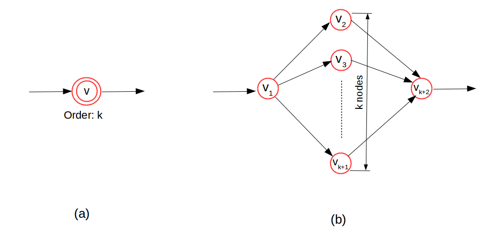
Composite node. A composite node of order is a gadget of nodes as shown in Figure 14. A composite node can have only one incoming edge and only one outgoing edge. Without using any extra resource, a composite node of order takes units of time to finish its activities. This is because there is one write operation on vertex , one write operation on vertex and write operations on vertex . Using units of resource with the -way splitting function, all activities can be completed in time. Similarly using units of resource with recursive binary splitting function, all activities will be completed in time. Thus using units of resource, composite node takes units of time using either function.
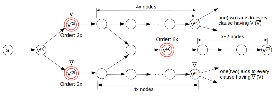
Variable gadget. The gadget for variable consists of composite nodes and other nodes as shown in Figure 14. Composite nodes and are of order . Composite node is of order . There is a chain of nodes from to inclusive. Similarly there is a chain of nodes from to inclusive. We will see that unless a variable gadget gets exactly units of resource, its makespan will be greater than which we will use as the target makespan later in our hardness proof. The values of and will be described shortly. Sending units of resource to node (Figure 14) corresponds to setting the variable to TRUE and sending units of resources to corresponds to setting to FALSE. We will see that sending one unit of resource to and one unit of resource to will make the makespan greater than the target makespan.
Clause gadget. The gadget corresponding to clause has vertices () as shown in Figure 14. Vertices and are composite nodes each of order . If clause has three literals and , then vertex is connected to the vertices and . These vertices correspond to and respectively. Vertex is connected to and . These vertices correspond to and . Vertex is connected to and . These vertices correspond to and . There are composite nodes and each of order . There is a chain of vertices from to each vertex in . We define the “earliest finish time” of a node as the time when all the write operations at are finished.
In a valid assignment of 1-in-3SAT, we show that for each clause , exactly vertices of and will have earliest finish time of and the other one will have earliest finish time of . (Table 3)
Value of . There is only one vertex () with out-degree zero in every variable gadget . Also, in every clause gadget , there are three vertices and , each with zero out-degree. So, if we connect all such vertices to the sink vertex , then in-degree at will be . Let be the smallest power of such that . We perform a recursive binary splitting at vertex . Let be the height of the binary splitting at where . To make , we define . Hence, the path from any vertex from to sink will take time .
Truth value assignment. Setting variable to TRUE implies sending units of resource through composite vertex . The corresponding earliest finish time at vertex is and at vertex is . Similarly, setting variable to FALSE implies sending units of resource through vertex . The corresponding earliest finish time at vertex is and at vertex is .
Lemma 4.5.
There exists a solution to the input instance of 1-in-3SAT iff there exists a valid flow of resource through the reduced DAG achieving a makespan of at most using at most units of resource.
Proof.
Forward direction. We now prove that if there is a solution to the 1-in-3SAT instance with variables and clauses, then the reduced DAG has a makespan of with units of resource.
If a variable is set to TRUE, then we allow units of resource to flow through vertex along the path , otherwise, we allow units of resource to flow through vertex along the path . Assigning TRUE to variable implies that the earliest finish times at vertex and are and , respectively. Also, the earliest finish time at vertex is . In Figure 14, there are writers from variable gadgets that write on each of the nodes in . If there are multiple writers ready to write to the same vertex at the same time, we serialize the write operations. For example, if and , then the writer from variable gadget is ready to write at time . The writers from and are ready to write at time . Hence, all three write operations can be completed at time . From Table 3, it is evident that in clause , if only one literal is TRUE and the other two are FALSE, then among and only one vertex has an earliest finish time of and the other two have . The vertex with starting time , can finish the activity corresponding to composite node (one of and ) of order , in another units of time without using any resource. Hence, it will finish at time . Each of the other two vertices with earliest finish time of takes units of resource flowing from vertex and finishes the composite node’s activity at time . There is a chain of nodes from the source vertex to each of the vertices in . Thus, the earliest finish time at each of those three vertices is . Together, with units of time to sink vertex , the total makespan is .
Backward direction. To achieve a makespan of , every variable gadget requires units of resource and each clause gadget requires , otherwise the makespan will be which is larger than because . Also, any resource used in a variable gadget cannot be used further in any other variable or clause gadget because the resource can be reused over a path only. Similarly, any resource used in any clause gadget cannot be reused in any other gadget. Only one vertex that is either or , will have the earliest finish time of . Both cannot be , as there is only units of resource per variable gadget. Both cannot be as in a clause where the literal or is present, there is an edge from either or to each of and . This requires clause gadget to get units of resource to achieve a makespan . But each clause gadget can have exactly units of resource. Thus, for every variable , for it to be a valid assignment, is set to either TRUE or FALSE. From Table 3, if a clause has exactly one TRUE literal, then one of the vertices from and has the earliest finish time of and the other two have . This requires to have units of resource to achieve the earliest finish time at each of the vertices from . This can be achieved by assigning units of resource to those two composite nodes (from and ) that start executing at time . The composite node that can start at time does not use any extra resource. If the clause does not have exactly one TRUE literal, then the clause gadget would require units of resource to achieve the target makespan. However, we just argued that each clause gadget can have exactly units of resource. Thus, each clause has exactly one TRUE literal and the 1-in-3SAT instance is also satisfied. ∎

4.3. Underlying Bounded Treewidth Graph
Let be the undirected graph obtained by ignoring the directedness of the edges of a given DAG . In the case that is a graph of bounded treewidth,222Recall that a tree decomposition of a graph is a tree with nodes , , satisfying: (1) ; (2) For edge there exists a with ; (3) For any two nodes, and , in , if node is in the (unique) path between and in , then . The width of the tree decomposition is , and the treewidth of is the minimum width over all tree decompositions of . we show that the offline minimum-makespan and minimum-resource problems on are (weakly) NP-hard. (Note that Theorem 4.1 proving the strong NP-hardness of the problems does not assume that the underlying undirected graph is of bounded treewidth.)
Theorem 4.6.
It is weakly NP-hard to decide if there exists a solution to the (offline) discrete resource-time tradeoff problem, with resource reuse over paths and a non-increasing duration function, satisfying a resource bound and a makespan bound , provided the undirected graph obtained by ignoring the directedness of the edges of the input DAG is of bounded treewidth.
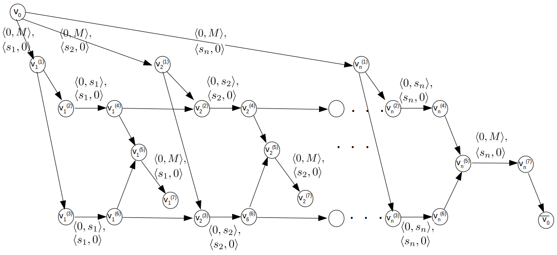
The proof of this theorem is based on a reduction from Partition(Garey and Johnson, 1979). The construction is shown in Figure 16. The input instance is a set of positive integers; let . The Partition problem asks if there is a partition of into subsets and such that the sums of the values in the two subsets are the same (i.e., exactly ). In this construction we have a total of resources to allocate in our program. The value is chosen to be greater than , the target makespan, ensuring that memory resources must be allocated to these nodes. This ensures that at least units of resource pass through each , constructing our numbers. From each there are two choices of nodes, and , to pass the resources onto each of which will either utilize resources or increase the makespan on that path by . The pair also funnel the resources into a sink vertex with a potential makespan cost of which ensures that their resources cannot be passed along to nodes and to the right (i.e., ). Thus the top and bottom paths represent our two sets and for each we must allocate makespan to either the top or the bottom path. Thus a total makespan of can only be achieved iff there is a partition of the ’s into two sets such that each set sums to .
To see that the constructed graph has bounded treewidth, let , where . Vertices for are connected to the sink vertex . Then has a tree decomposition with nodes , , as shown in Figure 16, with defined as follows: ; , for . We claim that is a valid tree decomposition. It is evident that . From the construction of , it is clear that, for each edge of the graph , there exists a node with . For any and , with and , we have , and, for any node (), on the path between and , we have and , so that . Thus, is a valid tree decomposition, and it has width 15 (), so the treewidth of is at most .
5. Conclusion
In this paper we introduce the discrete resource-time tradeoff problem with resource reuse in which each unit of resource is routed along a source to sink path and is possibly used and reused to expedite activities encountered along that path. We consider two different objective functions: (1) optimize makespan given a limited resource budget and (2) optimize resource requirement given a target makespan.
Our original motivation came from a desire to mitigate the cost of data races in shared-memory parallel programs by using extra space to reduce the time it takes to perform conflict-free write operations to shared memory locations. We consider three duration functions: general non-increasing function for the general resource-time question, and recursive binary reduction and multiway (k-way) splitting for the space-time case.
We present the first hardness and approximation hardness results as well as the first approximation algorithms for our problems. We show that the makespan optimization problem is strongly NP-hard under all three duration functions. When the duration function is general non-increasing we also show that it is strongly NP-hard to achieve an approximation ratio less than for the makespan optimization problem and less than for the resource optimization problem. We give a bi-criteria (resource, makespan) approximation algorithm for that same duration function, where . We present improved approximation ratios for the recursive binary reduction function and the multiway (-way) splitting functions.
Acknowledgements.
This work is supported in part by NSF grants CCF-1439084, CCF-1526406, CNS-1553510, IIS-1546113 and US-Israel Binational Science Foundation grant number 2016116.References
- (1)
- TCM (ools) Google gperftools. Fast, multi-threaded malloc() and nifty performance analysis tools. http://code.google.com/p/gperftools/.
- lla (lloc) llalloc. Lockless memory allocator. http://locklessinc.com/.
- Aigner et al. (2015) Martin Aigner, Christoph M Kirsch, Michael Lippautz, and Ana Sokolova. 2015. Fast, multicore-scalable, low-fragmentation memory allocation through large virtual memory and global data structures. In ACM SIGPLAN Notices, Vol. 50. ACM, 451–469.
- Akkan et al. (2005) Can Akkan, Andreas Drexl, and Alf Kimms. 2005. Network decomposition-based benchmark results for the discrete time–cost tradeoff problem. European Journal of Operational Research 165, 2 (2005), 339–358.
- Berger et al. (2000) Emery D Berger, Kathryn S McKinley, Robert D Blumofe, and Paul R Wilson. 2000. Hoard: A scalable memory allocator for multithreaded applications. In ACM SIGARCH Computer Architecture News, Vol. 28. ACM, 117–128.
- Blayo et al. (1999) Eric Blayo, Laurent Debreu, Gregory Mounie, and Denis Trystram. 1999. Dynamic load balancing for ocean circulation model with adaptive meshing. In European Conference on Parallel Processing. Springer, 303–312.
- Board (1997) OpenMP Architecture Review Board. 1997. OpenMP: A Proposed Industry Standard API for Shared Memory Programming. White Paper (1997). url: http://www.openmp.org/specs/mp-documents/paper/paper.ps.
- De et al. (1995) Prabuddha De, E James Dunne, Jay B Ghosh, and Charles E Wells. 1995. The discrete time-cost tradeoff problem revisited. European Journal of Operational Research 81, 2 (1995), 225–238.
- De et al. (1997) Prabuddha De, E James Dunne, Jay B Ghosh, and Charles E Wells. 1997. Complexity of the discrete time-cost tradeoff problem for project networks. Operations research 45, 2 (1997), 302–306.
- Du and Leung (1989) Jianzhong Du and Joseph Y-T Leung. 1989. Complexity of scheduling parallel task systems. SIAM Journal on Discrete Mathematics 2, 4 (1989), 473–487.
- Dutot et al. (2004) Pierre-François Dutot, Grégory Mounié, and Denis Trystram. 2004. Scheduling parallel tasks: Approximation algorithms.
- Feng and Leiserson (1999) Mingdong Feng and Charles E Leiserson. 1999. Efficient detection of determinacy races in Cilk programs. Theory of Computing Systems 32, 3 (1999), 301–326.
- Frigo et al. (2009) Matteo Frigo, Pablo Halpern, Charles E Leiserson, and Stephen Lewin-Berlin. 2009. Reducers and other Cilk++ hyperobjects. In Proceedings of the twenty-first annual ACM Symposium on Parallelism in Algorithms and Architectures. ACM, 79–90.
- Fulkerson (1961) Delbert R Fulkerson. 1961. A network flow computation for project cost curves. Management science 7, 2 (1961), 167–178.
- Garey and Johnson (1979) Michael R. Garey and David S. Johnson. 1979. Computers and Intractability: A Guide to the Theory of NP-Completeness. W. H. Freeman & Co., New York, NY, USA.
- Henzinger et al. (2013) Thomas A Henzinger, Christoph M Kirsch, Hannes Payer, Ali Sezgin, and Ana Sokolova. 2013. Quantitative relaxation of concurrent data structures. In ACM SIGPLAN Notices, Vol. 48. ACM, 317–328.
- Jansen and Zhang (2006) Klaus Jansen and Hu Zhang. 2006. An approximation algorithm for scheduling malleable tasks under general precedence constraints. ACM Transactions on Algorithms (TALG) 2, 3 (2006), 416–434.
- Kelley Jr (1961) James E Kelley Jr. 1961. Critical-path planning and scheduling: Mathematical basis. Operations research 9, 3 (1961), 296–320.
- Kelley Jr and Walker (1959) James E Kelley Jr and Morgan R Walker. 1959. Critical-path planning and scheduling. In Papers presented at the December 1-3, 1959, eastern joint IRE-AIEE-ACM computer conference. ACM, 160–173.
- Lenstra and Rinnooy Kan (1978) Jan Karel Lenstra and AHG Rinnooy Kan. 1978. Complexity of scheduling under precedence constraints. Operations Research 26, 1 (1978), 22–35.
- Lepère et al. (2002) Renaud Lepère, Grégory Mounié, and Denis Trystram. 2002. An approximation algorithm for scheduling trees of malleable tasks. European Journal of Operational Research 142, 2 (2002), 242–249.
- Lepere et al. (2002) Renaud Lepere, Denis Trystram, and Gerhard J Woeginger. 2002. Approximation algorithms for scheduling malleable tasks under precedence constraints. International Journal of Foundations of Computer Science 13, 04 (2002), 613–627.
- Möhring (1989) Rolf H Möhring. 1989. Computationally tractable classes of ordered sets. In Algorithms and order. Springer, 105–193.
- Netzer and Miller (1992) Robert HB Netzer and Barton P Miller. 1992. What are race conditions?: Some issues and formalizations. ACM Letters on Programming Languages and Systems (LOPLAS) 1, 1 (1992), 74–88.
- Panagiotakopoulos (1977) D Panagiotakopoulos. 1977. A CPM time-cost computational algorithm for arbitrary activity cost functions. INFOR: Information Systems and Operational Research 15, 2 (1977), 183–195.
- Phillips Jr and Dessouky (1977) Steve Phillips Jr and Mohamed I Dessouky. 1977. Solving the project time/cost tradeoff problem using the minimal cut concept. Management Science 24, 4 (1977), 393–400.
- Reinders (2007) James Reinders. 2007. Intel Threading Building Blocks: outfitting C++ for multi-core processor parallelism. O’Reilly Media, Inc.
- Robinson (1975) Don R Robinson. 1975. A dynamic programming solution to cost-time tradeoff for CPM. Management Science 22, 2 (1975), 158–166.
- Schaefer (1978) Thomas J Schaefer. 1978. The complexity of satisfiability problems. In Proceedings of the tenth annual ACM symposium on Theory of computing. ACM, 216–226.
- Schneider et al. (2006) Scott Schneider, Christos D Antonopoulos, and Dimitrios S Nikolopoulos. 2006. Scalable locality-conscious multithreaded memory allocation. In Proceedings of the 5th international symposium on Memory management. ACM, 84–94.
- Shavit (2011) Nir Shavit. 2011. Data structures in the multicore age. Commun. ACM 54, 3 (2011), 76–84.
- Skutella (1998) Martin Skutella. 1998. Approximation algorithms for the discrete time-cost tradeoff problem. Mathematics of Operations Research 23, 4 (1998), 909–929.
- Turek et al. (1992) John Turek, Joel L Wolf, and Philip S Yu. 1992. Approximate algorithms scheduling parallelizable tasks. In Proceedings of the fourth annual ACM Symposium on Parallel Algorithms and Architectures. ACM, 323–332.
Appendix
Appendix A Alternate hardness proof from numerical 3D matching
We give a polynomial-time reduction from the numerical 3-dimensional matching problem to the discrete resource-time tradeoff problem (with resource reuse over paths and a non-increasing duration function).
Numerical 3-dimensional matching problem:
Given
and , partition into triples of equal sum .
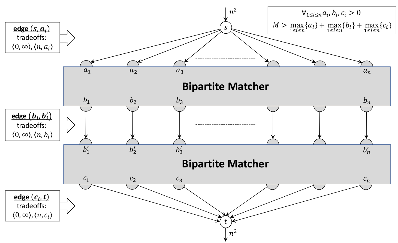
Given an instance of the numerical 3D matching problem, we create a DAG with source and sink as shown in Figure 18. For each , there is an edge in . The space-time tradeoff function at edge is . Recall that, this means that with zero resource, it takes infinite time to finish the activity and with units of resource it finishes in time . We create a gadget that has incoming edges and outgoing edges. We call the gadget a bipartite matcher (Figure 18) as it matches (a mapping) the incoming edges to the outgoing edges. We describe the bipartite matcher in the next paragraph. For each , there is an edge in . The tradeoff function at edge is . We put all the edges to a bipartite matcher as its incoming edges. For each , there is an edge in . The tradeoff function at edge is .
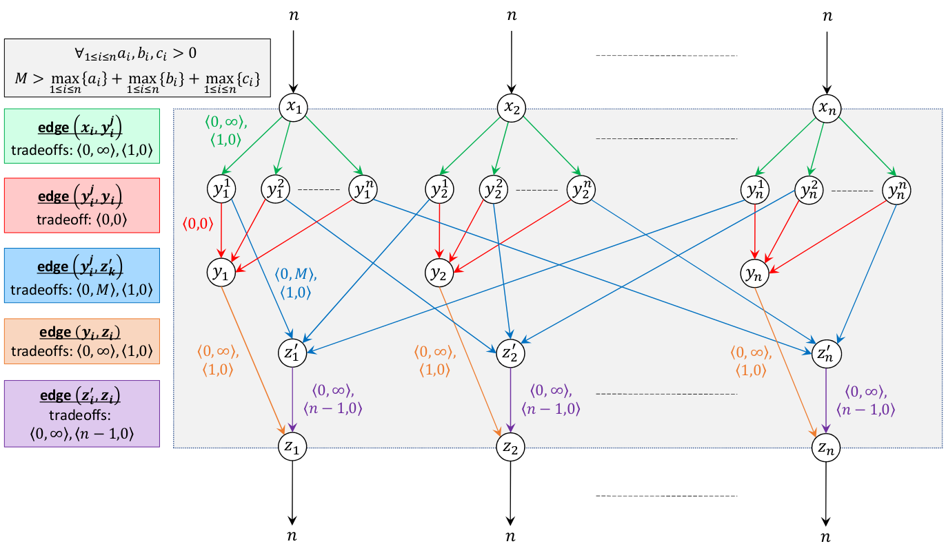
The bipartite matcher gadget. The gadget has incoming edges at vertices and outgoing edges from . It maps the vertices from to those in . The mapping is one to one. This works as follows. There are units of incoming resource at each vertices . Every outgoing edge from () has a tradeoff function . Hence, each of the outgoing edges from gets one unit of resource. The tradeoff function at edge is which forces to send one unit of resource to . The tradeoff function at edge is . Thus, if sends one unit of resource to , it cannot send any resource to forcing the activity to take units of time to finish. Here, . The tradeoff function at edge is . There are incoming edges to . Out of these incoming edges, edges flow units of resource to which are then used for the activity at .
We now show the mapping through an example. Suppose is mapped to . Then the corresponding flow is as follows: one unit of resource flows from to . As the total incoming flow of resource at vertex is one, no resource flows from to . However, one unit of resource flows from each except to . The earliest start time along path is while that along path for is . This makes the earliest start time at , . This holds true because . Also, units of resource flow to and they are used for the activity to finish in time . Observe that no except can send resource to . The gadget has a total resource-inflow of . Each of requires units of resource that sums up to units of resource. Each of requires one unit of resource, that sum up to units of resource. If two of sends a unit of resource each to , then the total resource left to be used by all is at most . Thus at least one of won’t get units of resource and will take infinite time. Hence, mapping to corresponds to flowing one unit of resource from to and vice-versa; this makes a one-to-one mapping from to .
Lemma A.1.
There exists a solution to a input instance of numerical 3D matching if and only if there exists a valid flow of resource in the DAG such that the makespan is with resource bound .
Proof.
If there is a solution in the input instance of numerical 3D matching, then there are sets, each of type such that . We use first bipartite matcher gadgets to map to and the second bipartite matcher to map to . Each bipartite matcher contributes in the makespan. and adds to the makespan. Thus the makespan is eaxctly .
If the reduced DAG admits a makespan of using units of resource, then there is also a solution to the input instance of numerical 3D matching. From the construction of bipartite 3D matching, there is a one-to-one mapping from to and from to . As the makespan is and each bipartite matcher contributes to the makespan, this gives a solution to numerical 3D matching. ∎