Semi-implicit methods for the dynamics of elastic sheets

Abstract

Recent applications (e.g. active gels and self-assembly of elastic sheets) motivate the need to efficiently simulate the dynamics of thin elastic sheets. We present semi-implicit time stepping algorithms to improve the time step constraints that arise in explicit methods while avoiding much of the complexity of fully-implicit approaches. For a triangular lattice discretization with stretching and bending springs, our semi-implicit approach involves discrete Laplacian and biharmonic operators, and is stable for all time steps in the case of overdamped dynamics. For a more general finite-difference formulation that can allow for general elastic constants, we use the analogous approach on a square grid, and find that the largest stable time step is two to three orders of magnitude greater than for an explicit scheme. For a model problem with a radial traveling wave form of the reference metric, we find transitions from quasi-periodic to chaotic dynamics as the sheet thickness is reduced, wave amplitude is increased, and damping constant is reduced.

I Introduction

In recent years there have been various studies of how spatial variations in the composition of a thin sheet can produce global conformational changes. Examples include the appearance of spontaneous curvature due to strain variations across the thickness of the sheet calladine:1983a ; freund:2004a ; armon:2011a or non-Euclidean reference metrics induced by in-plane strain variations audoly:2003a ; santangelo:2009a ; gemmer:2011a ; sharon:2012a ; sharon:2016a . A theory of incompatible elastic plates efrati:2009a ; efrati:2013a has been developed to determine equilibrium configurations of such sheets. Related approaches have been used to develop self-folding origami gels na:2015a . A catalog of responsive materials are now available for investigating the mechanics of thin sheets, including non-uniform responsive gel sheets klein:2007a ; kim:2012a ; wu:2013a , sheets of nematic elastomers with a non-uniform director field ware:2015a ; white:2015a , responsive gels combined with oriented micro-rods gladman:2016a , and sheets in confined geometries lin:2009a ; roman:2010a ; aharoni:2010a ; paulsen:2017a .

The dynamics of responsive gel sheets were the focus of work by Yoshida and collaborators, who synthesized a gel that locally swells in response to chemical waves propagating entirely within the gel  yoshida:1996a . They used self-oscillating gels in various narrow strip geometries to make a variety of soft machines maeda:2007a ; tabata:2002a ; tabata:2003a ; maeda:2008a ; shiraki:2012a . The Balazs group used poroelastic simulations of self-oscillating gels to demonstrate additional examples of soft machines with uniaxial bending or isotropic swelling yashin:2006a ; kuksenok:2007a ; yashin2007theoretical ; kuksenok:2014b . Here we will focus on simulating a simple but extensively-studied model, a thin elastic sheet driven by changes in its equilibrium metric. We will present an efficient semi-implicit time-stepping algorithm for the case of overdamped dynamics, a representative case with the same form of numerical stiffness as more detailed fluid-elastic and fluid-poroelastic models. The approach is also useful in other applications where the dynamics of thin elastic sheets are important, such as the self-assembly of thin sheets under magnetic forces boncheva2005magnetic ; Alben2007saf , and the the rolling of actuated bilayers alben2011edge ; Alben2015bending .

A related problem is simulating the dynamics of fluid membrane vesicles with surface tension veerapaneni2011fast . Here a similar time-step constraint arises for bending forces, while the thin elastic sheets considered in the present work also have stiffness due to stretching forces. Like veerapaneni2011fast , we develop a semi-implicit time-stepping approach for computational efficiency, though our formulation differs due to the different mechanical forces.

In general, a semi-implicit (or implicit-explicit) time discretization writes some of the terms (typically those with the highest spatial derivatives) implicitly, to improve time-step constraints for stability rosenbrock1963some ; gottlieb1977numerical ; Hou1994removing ; desbrun1999interactive ; eberhardt2000implicit ; Hou2001boundary ; selle2008mass ; Alben2008implicit ; alben2009simulating . The implicit terms are typically linear in the unknowns at the current time step, so they can be solved directly at each time step, avoiding some of the complication and computational expense of nonlinear iterative solvers (e.g. Newton-type methods) in fully implicit discretizations chen2018physical . If the linearized implicit term is sufficiently large in comparison to the explicit terms, the semi-implicit method may be stable for a wide range of time steps. For nonlinear PDEs, a somewhat empirical approach to formulating schemes, based on analogies with time-stepping for simpler linear PDEs, is often necessary.

In this work we begin with Seung and Nelson’s discretization of elastic sheets by bending and stretching springs on a triangular lattice Seung:1988 . We use the approach of desbrun1999interactive ; selle2008mass to split the stretching force into an implicit linear term corresponding to zero-rest-length springs, and a nonlinear remainder. The implicit stretching term is proportional to a discrete Laplacian matrix multiplying the current sheet position. To stabilize the bending force, we add an implicit bending term that is proportional to a discrete biharmonic matrix multiplying the current sheet position. The resulting method appears to be stable for all time steps. To allow for general elastic constants, we formulate a finite-difference discretization of the elastic energy with the analogous semi-implicit approach. We validate and compare the methods on test problems with internal in-plane stretching forces (nontrivial equilibrium metrics) and study the effects of basic physical parameters on the sheets’ dynamics.

II Elastic sheet

We consider a thin sheet or bilayer that undergoes large time-dependent deformations due to internal forces (from a prescribed, time- and space-varying reference metric). We assume the sheet obeys linear (Hookean) elasticity, but that the midsurface (the set of points located midway through the sheet in the thickness direction) can be an arbitrary smooth time-dependent surface, so elastic forces depend nonlinearly on its position. The extension of the Kirchhoff-Love (and Föppl-von-Kármán) models of elastic plates to nonflat reference metrics and/or large deformations with smooth midsurfaces has been called the Koiter shell theory koiter1966nonlinear ; ciarlet2000modele ; vetter2013subdivision or the theory of non-Euclidean plates efrati:2007a ; efrati:2009a . Here we mainly follow the latter’s notation.

The elastic energy involves stretching and bending energy terms determined by the position of the body, $\mathbf{r}(\mathbf{x})$. Here $\mathbf{r}$ lies in $\mathbb{R}^{3}$, as does the material coordinate $\mathbf{x}=(x_{1},x_{2},x_{3})$. In the classical situation, the sheet has a zero-energy flat state $\mathbf{r}(\mathbf{x})=\mathbf{x}$, where $x_{3}$ lies in the interval $[-h/2,h/2]$ ($h$ is the sheet thickness, much smaller than the other dimensions), and $x_{1}$ and $x_{2}$ lie in a planar region, the same for each $x_{3}$. For a small line of material $\mathbf{\Delta x}=\tilde{\mathbf{x}}-\mathbf{x}$ connecting two material points $\tilde{\mathbf{x}}$ and $\mathbf{x}$, its squared length on the undeformed surface is $dl^{2}=\Delta x_{i}\Delta x_{i}$ (with summation over repeated indices). Denote the squared length on the deformed surface $\mathbf{r}(\mathbf{x})$ by $dl^{\prime 2}$. Using the Taylor series of $\mathbf{r}(\mathbf{x})$ up to first derivatives we have

$$dl^{\prime 2}-dl^{2}=2\epsilon_{ij}\Delta x_{i}\Delta x_{j}.$$ (1)

Here $\epsilon_{ij}$ is the strain tensor,

$$\epsilon_{ij}=\frac{1}{2}\left(g_{ij}-\delta_{ij}\right).$$ (2)

where

$$g_{ij}=\frac{\partial r_{k}}{\partial x_{i}}\frac{\partial r_{k}}{\partial x_{j}}$$ (3)

is the metric tensor. For curved shells or active materials, the rest state may be curved and/or time-varying, in which case the reference metric, $\delta_{ij}$ in (2), becomes $\bar{g}_{ij}(\mathbf{x},t)$, a time- and space-varying function determined for example by chemical activity yoshida:1996a ; yashin:2006a ; klein:2007a :

$$\epsilon_{ij}=\frac{1}{2}\left(g_{ij}-\bar{g}_{ij}(\mathbf{x},t)\right).$$ (4)

The reference metric is assumed to take the form

$$\bar{g}=\begin{pmatrix}\bar{g}_{11}&\bar{g}_{12}&\hfill 0\cr\bar{g}_{21}&\bar{g}_{22}&\hfill 0\cr 0&0&\hfill 1\end{pmatrix}$$ (5)

with upper 2-by-2 reference metric $\bar{g}_{\alpha\beta}$. The dependence on out-of-plane components ($\bar{g}_{\alpha 3},\bar{g}_{3\alpha}$) is trivial, so shearing though the plate thickness is not imposed and expansion/contraction in the thickness direction occurs only passively, due to the Poisson ratio effect. The components of the metric $g_{i3}$ for $i=1,2,3$ are determined by the Kirchhoff-Love assumptions of no shearing in planes through the thickness, and no stress in the thickness direction. The result is $g_{\alpha 3}=g_{3\alpha}=0$ for $\alpha=1,2$, and $g_{33}=1$ efrati:2009a .

We may write the energy in terms of the midsurface deformation by expanding $g_{\alpha\beta}$ about the sheet midsurface $x_{3}=0$. We obtain, at leading order, its thickness-average $a_{\alpha\beta}$ and its thickness-gradient efrati:2009a :

$$g_{\alpha\beta}=a_{\alpha\beta}-2x_{3}b_{\alpha\beta}+O(h^{2}).$$ (6)

Here $a_{\alpha\beta}$ is the upper 2-by-2 part of the metric tensor (3) evaluated at the sheet midsurface, $x_{3}=0$. The thickness-gradient is written in terms of $b_{\alpha\beta}$, the second fundamental form

$$b_{\alpha\beta}=\frac{\partial^{2}r_{k}}{\partial x_{\alpha}\partial x_{\beta}}n_{k}$$ (7)

also evaluated at the sheet midsurface, $x_{3}=0$, with $n_{k}$ the components of the midsurface unit normal vector $\mathbf{n}$. For the reference metric $\bar{g}$, we write $\bar{a}$ and $\bar{b}$ for the corresponding terms in the expansion about the midsurface.

For an isotropic sheet with Young’s modulus $E$, Poisson ratio $\nu$, and thickness $h$, the elastic energy per unit volume is

$$w=\frac{1}{2}\bar{A}^{\alpha\beta\gamma\delta}\epsilon_{\alpha\beta}\epsilon_{\gamma\delta},$$ (8)

a quadratic function of the in-plane components of the strain tensor in (4) with elasticity tensor

$$\bar{A}^{\alpha\beta\gamma\delta}=\frac{E}{1+\nu}\left(\frac{\nu}{1-\nu}\bar{g}^{\alpha\beta}\bar{g}^{\gamma\delta}+\bar{g}^{\alpha\gamma}\bar{g}^{\beta\delta}\right)$$ (9)

where the entries of $\bar{g}^{\alpha\beta}$ are those of $\bar{g}_{\alpha\beta}^{-1}$. Integrating $w$ over the sheet thickness, the energy per unit midsurface area is

$$w_{2D}=\int_{-h/2}^{h/2}wdx_{3}=w_{s}+w_{b}+h.o.t.,$$ (10)

a sum of stretching energy per unit area

$$w_{s}=\frac{h}{8}A^{\alpha\beta\gamma\delta}\left(a_{\alpha\beta}-\bar{a}_{\alpha\beta}\right)\left(a_{\gamma\delta}-\bar{a}_{\gamma\delta}\right)$$ (11)

and bending energy per unit area

$$w_{b}=\frac{h^{3}}{24}A^{\alpha\beta\gamma\delta}\left(b_{\alpha\beta}-\bar{b}_{\alpha\beta}\right)\left(b_{\gamma\delta}-\bar{b}_{\gamma\delta}\right).$$ (12)

in terms of the midsurface elasticity tensor

$$A^{\alpha\beta\gamma\delta}=\frac{E}{1+\nu}\left(\frac{\nu}{1-\nu}\bar{a}^{\alpha\beta}\bar{a}^{\gamma\delta}+\bar{a}^{\alpha\gamma}\bar{a}^{\beta\delta}\right),$$ (13)

and higher order terms in $h$. The total elastic energy is, to leading order in $h$,

$$W=W_{s}+W_{b}\;,\quad W_{s}=\iint w_{s}\sqrt{|\bar{a}|}dx_{1}dx_{2}\;,\quad W_{b}=\iint w_{b}\sqrt{|\bar{a}|}dx_{1}dx_{2}.$$ (14)

$W$ is a function of the midsurface configuration, $\mathbf{r}(x_{1},x_{2},0)$ and midsurface reference metric $\bar{a}$.

III Sheet dynamics

The sheet midplane evolves according a force balance equation, where the elastic force per unit area $\mathbf{f}$ acting at a point on the midplane is a sum of stretching and bending forces per unit area:

$$\mathbf{f}=\mathbf{f}_{s}+\mathbf{f}_{b}=\delta w_{s}/\delta\mathbf{r}+\delta w_{b}/\delta\mathbf{r}$$ (15)

given by taking the variation of $w_{s}+w_{b}$ with respect to $\mathbf{r}$. For a sheet moving in Stokes flow (i.e. at zero Reynolds number) the elastic forces would be balanced by external fluid forces which depend linearly on the sheet velocity veerapaneni2011fast :

$$\frac{\partial\mathbf{r}}{\partial t}=\mathcal{S}[\mathbf{f}_{s}+\mathbf{f}_{b}](\mathbf{r}).$$ (16)

where $\mathcal{S}$ is the Stokes operator

$$\mathcal{S}[\mathbf{f}](\mathbf{r})=\int G(\mathbf{r},\mathbf{r^{\prime}})\mathbf{f}(\mathbf{r^{\prime}})dA(\mathbf{r^{\prime}}),\quad G(\mathbf{r},\mathbf{r^{\prime}})=\frac{1}{8\pi\mu}\left(\frac{1}{\|\rho\|}\mathbf{I}+\frac{\rho\otimes\rho}{\|\rho\|^{3}}\right),\quad\rho\equiv\mathbf{r}-\mathbf{r^{\prime}}.$$ (17)

In this work, we consider a simplification of (16) which has similar numerical stiffness issues: overdamped dynamics, in which the Stokes operator is replaced with a multiple of the identity:

$$\mu\frac{\partial\mathbf{r}}{\partial t}=\mathbf{f}.$$ (18)

Here $\mu$ is a parameter that can be used to model the effects of internal and external damping. The equation can also be used to identify equilibria as a gradient descent method nocedal2006numerical with time playing a nonphysical role. Extensions of (18) including the inertia of the sheet or a surrounding fluid will add a dependence on $\partial^{2}\mathbf{r}/\partial t^{2}$. When discretized, the $~{}\Delta t^{-2}$ dependence of such terms will improve the time-step constraint compared to the overdamped problem, for explicit schemes hairer1987solving . In this work, we develop a semi-implicit approach for (18), which should also apply with more detailed forms of internal and external damping/forcing, e.g. from a fluid. In the subsequent computational results we nondimensionalize the sheet lengths by the radius or half-width $R$ (e.g. for hexagonal and square sheets), energy by the bending energy scale $Eh^{3}/12$, and time by the period of $\bar{g}_{\alpha\beta}(\mathbf{x},t)$ (assumed to be time-periodic). These choices define dimensionless versions of all the parameters (e.g. $\mu$).

IV Triangular lattice with stretching and bending springs

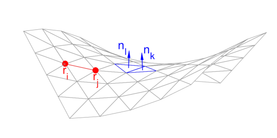
Figure 1: Triangular lattice mesh with examples of elements in the elastic energy: adjacent vertices $\mathbf{r}_{i}$ and $\mathbf{r}_{j}$ (red) and adjacent face normals $\mathbf{n}_{k}$ and $\mathbf{n}_{l}$ (blue).

We first consider a simple model of an elastic sheet with material points connected by an equilateral triangular lattice mesh. Nearest neighbor points are connected by Hookean springs and the total stretching energy is a sum of the squares of nearest neighbor distances minus the local spring rest length $d_{ij}$:

$$U_{s}=\frac{K_{s}}{2}\sum_{i,j}(\|\mathbf{r}_{i}-\mathbf{r}_{j}\|-d_{ij})^{2},$$ (19)

with $K_{s}$ a stretching stiffness constant. A bending energy is applied to adjacent triangular faces based on the angles between the normals to the faces. The total bending energy is a sum over nearest neighbor pairs with bending stiffness constant $K_{b}$:

$$U_{b}=\frac{K_{b}}{2}\sum_{k,l}\|\mathbf{n}_{k}-\mathbf{n}_{l}\|^{2}=K_{b}\sum_{k,l}1-\mathbf{n}_{k}\cdot\mathbf{n}_{l}.$$ (20)

Seung and Nelson used this model to study buckling due to defects in elastic membranes Seung:1988 , and it was used by many other groups to study other deformations of thin sheets and shells due to defects and/or external forces gompper1997fluctuations ; lobkovsky1997properties ; lidmar2003virus ; vliegenthart2006forced ; katifori2010foldable ; couturier2013folding ; funkhouser2013topological ; Alben2015bending ; wan2017thermal , as well as polymerized and fluid membranes nelson2004statistical .

Seung and Nelson showed that for a lattice with $d_{ij}\equiv d$, a constant, as $d$ tends to 0 the stretching energy $U_{s}$ tends to that of an isotropic thin sheet with stretching rigidity $Eh=2K_{s}/\sqrt{3}$ and Poisson ratio $\nu=1/3$. The continuum limit of the bending energy contains two terms, one proportional to the mean curvature squared and the other proportional to the Gaussian curvature. The term involving mean curvature tends to that of an isotropic thin sheet with bending rigidity $Eh^{3}/12(1-\nu^{2})=\sqrt{3}K_{b}/2$. However, with this bending rigidity, the prefactor of the Gaussian curvature term is too large for $\nu>-1/3$ (too large by a factor of two at $\nu=1/3$) schmidt2012universal . Nonetheless, for many problems, the Gaussian curvature term plays a negligible role because it can be integrated to yield only boundary terms. For closed shells, the Gaussian curvature term integrates to a constant and thus does not affect the elastic forces lidmar2003virus . For open sheets (with boundaries), the equilibrium shape could be insensitive to the boundary shape or boundary conditions, particularly if the external or internal actuation is not localized at the boundary. In this work we will compare the model to a finite-difference discretization with $\nu=1/3$ in two cases, and find a very small difference in a case of static actuation (also found in another situation by didonna2002scaling ), and a somewhat larger difference in a case of dynamic actuation.

The triangular lattice sheet is useful computationally because it has a simple expression for the energy and motivates our semi-implicit approach for the more general finite difference discretization given subsequently. The elastic force on the triangular lattice is obtained by taking gradients of (19) and (20) with respect to vertex coordinates $\left\{\mathbf{r}_{i}\right\}$. The gradient of (19) with respect to $\mathbf{r}_{i}$ is

$$\nabla_{\mathbf{r}_{i}}U_{s}=K_{s}\sum_{\displaystyle j\in\mbox{nhbrs}(i)}(\|\mathbf{r}_{i}-\mathbf{r}_{j}\|-d_{ij})\frac{(\mathbf{r}_{i}-\mathbf{r}_{j})}{\|\mathbf{r}_{i}-\mathbf{r}_{j}\|}.$$ (21)

where nhbrs$(i)$ is the set of vertex neighbors to $i$. Following desbrun1999interactive ; selle2008mass we write the summand as a linear term plus a term with constant magnitude,

$$\nabla_{\mathbf{r}_{i}}U_{s}=K_{s}\sum_{\displaystyle j\in\mbox{nhbrs}(i)}\mathbf{r}_{i}-\mathbf{r}_{j}-d_{ij}\frac{(\mathbf{r}_{i}-\mathbf{r}_{j})}{\|\mathbf{r}_{i}-\mathbf{r}_{j}\|}.$$ (22)

To write the algorithms we define

$$\bm{r}=\left[\bm{r}_{x}^{\intercal},\bm{r}_{y}^{\intercal},\bm{r}_{z}^{\intercal}\right]^{\intercal}$$ (23)

as the vector of 3$N$ vertex coordinates, with $\bm{r}_{x}$, $\bm{r}_{y}$, and $\bm{r}_{z}$ the $N$-vectors of $x$-, $y$-, and $z$-coordinates. Thus $\mathbf{r}_{i}=\left[\left(\bm{r}_{x}\right)_{i},\left(\bm{r}_{y}\right)_{i},\left(\bm{r}_{z}\right)_{i}\right]^{\intercal}$. Also note that the italicized $\bm{r}\in\mathbb{R}^{3N}$ is different from the position function $\mathbf{r}(\mathbf{x})$ and a vertex on the discretized surface $\mathbf{r}_{i}$, both of which take values in $\mathbb{R}^{3}$. It turns out that the linear term in (22) can be written as the product of $K_{s}$ and a block diagonal matrix $\mathbf{L}$ with $\bm{r}$, where $\mathbf{L}$ has three blocks (along the diagonal), each of which is a discretized Laplacian on the triangular mesh with free-edge boundary conditions (see examples of stencils in figure 2, top row), a negative semidefinite matrix. Each block multiplies $\bm{r}_{x}$, $\bm{r}_{y}$, and $\bm{r}_{z}$, respectively. We treat the linear term implicitly and the constant-magnitude term explicitly. Collecting the terms (22) for all vertices $i$, we obtain the total stretching force. A semi-implicit first-order temporal discretization of (18) with stretching forces only is:

$$\mu A_{p}\frac{\bm{r}^{n+1}-\bm{r}^{n}}{\Delta t}=K_{s}\mathbf{L}\bm{r}^{n+1}+\mathbf{f}_{SE}(\bm{r}^{n})\;,\quad\left[\mathbf{f}_{SE}(\bm{r})_{i},\mathbf{f}_{SE}(\bm{r})_{N+i},\mathbf{f}_{SE}(\bm{r})_{2N+i}\right]^{\intercal}\equiv-K_{s}\sum_{\displaystyle j\in\mbox{nhbrs}(i)}d_{ij}\frac{(\mathbf{r}_{i}-\mathbf{r}_{j})}{\|\mathbf{r}_{i}-\mathbf{r}_{j}\|}.$$ (24)

Here $A_{p}=n_{p}\sqrt{3}d^{2}/12$ is the area per point on the undeformed lattice, with $n_{p}$ the number of triangles of which the point is a vertex, 6 for interior points and fewer for boundary points. $\mathbf{f}_{SE}(\bm{r})$ is the nonlinear term in (22), with 3$N$ entries, given on the right side of (24) for $i=1,\ldots,N$.

Now assume the spring rest lengths are bounded for all time: $d_{ij}\leq\bar{d}$, a constant, and each vertex has at most $p$ neighbors (6 for the triangular lattice). Rearranging (24) and using the boundedness of $\mathbf{f}_{SE}(\bm{r})$, we have an upper bound at time step $n+1$:

$$\left\|\bm{r}^{n+1}\right\| \leq \left\|(\mathbf{I}-\Delta tK_{s}\mathbf{L}/(\mu A_{p}))^{-1}\bm{r}^{n}\right\|+\left\|(\mathbf{I}-\Delta tK_{s}\mathbf{L}/(\mu A_{p}))^{-1}\mathbf{f}_{SE}(\bm{r}^{n})\right\|$$ (25)

$$\leq \left\|\bm{r}^{n}\right\|+K_{s}p\bar{d}$$ (26)

$$\leq \left\|\bm{r}^{0}\right\|+(n+1)K_{s}p\bar{d}.$$ (27)

So $\|\bm{r}^{n+1}\|$ grows at most linearly in time with this discretization. Empirically, the iteration appears to be bounded for all time steps for spring rest lengths $d_{ij}$ that are bounded in time. For comparison, a forward Euler discretization of (18) with stretching forces only results in

$$\bm{r}^{n+1}=\left(\mathbf{I}+\Delta tK_{s}\mathbf{L}/(\mu A_{p})\right)\bm{r}^{n}+\frac{\Delta t}{\mu A_{p}}\mathbf{f}_{SE}(\bm{r}^{n}).$$ (28)

Neglecting the rightmost term in (28), we have a 2D diffusion equation, and stability is possible only when the largest eigenvalue of $\mathbf{I}+\Delta tK_{s}\mathbf{L}/(\mu A_{p})$ is bounded in magnitude by 1. Since the eigenvalues of $\mathbf{L}\sim 1/\Delta x^{2}$ for lattice spacing $\Delta x$, this requires $\Delta t<C_{s}\mu A_{p}\Delta x^{2}/K_{s}$ for a constant $C_{s}$.

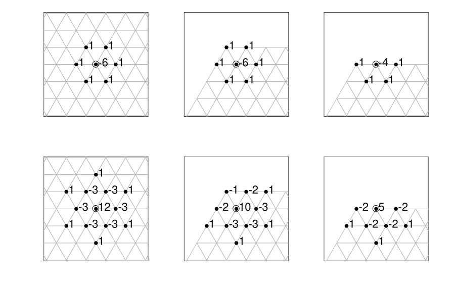
Figure 2: Examples of the stencils corresponding to a discrete Laplacian operator with free edge boundary conditions (one of the diagonal blocks of $\mathbf{L}$ defined below (22)) (top row), and $\tilde{\Delta}^{2}_{x_{1},x_{2}}$, a discrete biharmonic operator with free edge boundary conditions (bottom row), at different mesh points (circled) away from and near a boundary on the triangular lattice.

The gradient of the bending energy (20) with respect to a lattice vertex $\mathbf{r}_{i}$ is

$$\nabla_{\mathbf{r}_{i}}U_{b}=K_{b}\sum_{k,l}\sin{\theta_{kl}}\nabla_{\mathbf{r}_{i}}\theta_{kl},$$ (29)

using $\mathbf{n}_{k}\cdot\mathbf{n}_{l}=\cos{\theta_{kl}}$. The dihedral angle $\theta_{kl}$ depends on the four points in the union of the neighboring triangles $k$ and $l$ (see figure 1). Two of these points are the endpoints of the edge shared by the triangles. At each of the other two points, $\nabla_{\mathbf{r}_{i}}\theta_{kl}$ is directed along the normal to the triangle in which it lies, with magnitude equal to the reciprocal of its distance from the shared edge. At the endpoints of the shared edge, $\nabla_{\mathbf{r}_{i}}\theta_{kl}$ can be found by requiring that the net force and torque due to $\theta_{kl}$ is zero, which gives six equations (for the three components of net force and torque) in six unknowns (the forces on the two endpoints of the shared edge). The bending force $\mathbf{f}_{B}$ is a 3$N$-vector with components

$$\left[\mathbf{f}_{B}(\bm{r})_{i},\mathbf{f}_{B}(\bm{r})_{N+i},\mathbf{f}_{B}(\bm{r})_{2N+i}\right]^{\intercal}\equiv-\nabla_{\mathbf{r}_{i}}U_{b},\;i=1,\ldots,N,$$ (30)

similar to $\mathbf{f}_{SE}$ in (24). Our linearized approximation to the bending force is similar to that of veerapaneni2011fast . They write the terms with the highest spatial derivatives in the form $\mathcal{B}(\bm{r}^{n})\bm{r}^{n+1}$. Here $\mathcal{B}$ involves fourth derivatives with prefactors that include lower-order derivatives extrapolated to time step $n+1$ from previous time steps. In fact, we use a simpler expression: $\mathbf{B}\bm{r}^{n+1}$, where $\mathbf{B}$ is a block diagonal matrix with each of the three blocks equal to $D\tilde{\Delta}^{2}_{x_{1},x_{2}}$. Here $D$ is the bending modulus ($Eh^{3}/(12(1-\nu^{2}))$ in dimensional form, $1/(1-\nu^{2})$ in dimensionless form) and $\tilde{\Delta}^{2}_{x_{1},x_{2}}$ is the discretized biharmonic operator on the triangular lattice in the orthogonal material coordinates $x_{1}$ and $x_{2}$. If in-plane strain (shearing and dilation) are not very large, $x_{1}$ and $x_{2}$ are close to orthogonal arclength coordinates $s_{1}$, $s_{2}$ along the midplane surface. For any surface $\mathbf{X}(s_{1},s_{2})$ parametrized by orthogonal arclength coordinates $s_{1}$, $s_{2}$ we can write

$$\Delta^{2}_{s_{1},s_{2}}\mathbf{X}(s_{1},s_{2})=\Delta_{s_{1},s_{2}}(\kappa_{1}+\kappa_{2})\hat{\mathbf{n}}+N.$$ (31)

where $\kappa_{1}+\kappa_{2}$ is twice the mean curvature and $N=(\kappa_{1}+\kappa_{2})\Delta_{s_{1},s_{2}}\hat{\mathbf{n}}$ involves derivatives of $\mathbf{X}$ that are of lower order than those in the first term on the right hand side. The highest-derivative term in the continuum bending force is also the first term on the right hand side of (31) when the equilibrium metric is the identity (see weiner1978problem ; veerapaneni2011fast ). Thus the left hand side of (31) is a reasonable linear (and constant-coefficient) approximation to the bending force. A more accurate linear approximation to the bending operator could include corrections that take into account the nontrivial inverse equilibrium metric ($\bar{g}^{\alpha\beta}$ in (13)) and in-plane strain, e.g. by including nonuniform prefactors extrapolated from previous time steps. We find however that the constant-coefficient biharmonic is a sufficiently good approximation in the sense that it damps out spurious mesh-scale bending oscillations (as occurs with a fully explicit bending term) up to large-amplitude variations in the reference metric, $\approx 0.3$ in terms of an amplitude parameter $A$ defined in (34)–(36), below. With larger variations in the reference metric, the position vector remains bounded in time, but there is very large deformation and self-intersection even for the case of purely planar deformations, without bending forces. We explain how the discrete biharmonic operator $\tilde{\Delta}^{2}_{x_{1},x_{2}}$ is calculated in appendix A.

Semi-implicit (or implicit-explicit) schemes for cloth animation have sometimes left bending forces explicit, when they are much smaller than stretching forces eberhardt2000implicit . Considering a forward Euler discretization of (18) with bending forces only, and approximating the bending force by $\mathbf{B}\bm{r}^{n}$, stability requires $\Delta t<C_{b}\mu A_{p}\Delta x^{4}/K_{b}$ for a constant $C_{b}$, since the eigenvalues of $\mathbf{B}\sim 1/\Delta x^{4}$ for lattice spacing $\Delta x$. The ratio of bending to stretching time step constraints $\sim K_{s}\Delta x^{2}/K_{b}\sim\Delta x^{2}/h^{2}$, the square of the ratio of lattice spacing to sheet thickness. For the parameters used in this work, the stretching time step constraint is typically smaller, but not much smaller than the bending time constraint, so a semi-implicit approach needs to address both terms.

Our first-order semi-implicit discretization for sheet dynamics with both stretching and bending forces is:

$$\mu A_{p}\frac{\bm{r}^{n+1}-\bm{r}^{n}}{\Delta t}=K_{s}\mathbf{L}\bm{r}^{n+1}+\mathbf{f}_{SE}(\bm{r}^{n})+\mathbf{B}\bm{r}^{n+1}-\mathbf{B}\bm{r}^{n}+\mathbf{f}_{B}(\bm{r}^{n}).$$ (32)

The last two terms on the right hand side approximately cancel in the highest-derivative term, leaving the implicit bending term $\mathbf{B}\bm{r}^{n+1}$ as the dominant one. The second-order version with uniform time stepping (an approximate backward differentiation formula) is:

$$\mu A_{p}\frac{3\bm{r}^{n+1}-4\bm{r}^{n}+\bm{r}^{n-1}}{2\Delta t}=K_{s}\mathbf{L}\bm{r}^{n+1}+2\mathbf{f}_{SE}(\bm{r}^{n})-\mathbf{f}_{SE}(\bm{r}^{n-1})+\mathbf{B}\bm{r}^{n+1}-2\mathbf{B}\bm{r}^{n}+\mathbf{B}\bm{r}^{n-1}+2\mathbf{f}_{B}(\bm{r}^{n})-\mathbf{f}_{B}(\bm{r}^{n-1}).$$ (33)

For test problems that model the deformation and dynamics of active gel sheets driven by internal swelling yoshida:1996a ; yashin:2006a ; yashin2007theoretical ; klein:2007a , we construct a uniform triangular lattice with spacing $d$. We then set the dilatation factor $d_{ij}/d\equiv\eta$ to correspond to one of three examples: a static radial distribution, a unidirectional traveling wave, or a radial traveling wave of isotropic dilation/contraction:

$$\eta_{1}(x_{1},x_{2},t) = 1+A\cos\left({2\pi\left(k\sqrt{x_{1}^{2}+x_{2}^{2}}\right)}\right)$$ (34)

$$\eta_{2}(x_{1},x_{2},t) = 1+A\sin\left({2\pi\left(kx_{1}-t\right)}\right)$$ (35)

$$\eta_{3}(x_{1},x_{2},t) = 1+A\sin\left({2\pi\left(k\sqrt{x_{1}^{2}+x_{2}^{2}}-t\right)}\right).$$ (36)

The corresponding equilibrium metrics are

$$\bar{a}_{\alpha\beta}(x_{1},x_{2},t)=\eta^{2}(x_{1},x_{2},t)\delta_{\alpha\beta},$$ (37)

and we take zero reference curvature ($\bar{b}_{\alpha\beta}=0$) for simplicity. Before presenting results, we describe in the next section a more direct finite difference simulation that allows for more general elastic parameters than the triangular lattice model. However, the triangular lattice simulations have the advantage of remaining bounded in time for all time steps across wide ranges (several orders of magnitude) of values for the parameters ($h$, $A$, $k$, $\mu$) with large mesh sizes (hexagonal domains with $N$ = 3367 and 9241, for example). Simulations appear smooth up to strain amplitudes $A\sim 0.3$. Above this value, sheet shapes become jagged and self-intersect, but remain bounded in time. Hence the time step and lattice spacing are constrained only by the need to resolve the dynamics at a given parameter set. The method can also be used to converge to static equilibria, in which case the time step becomes a step length for a gradient descent algorithm. Here a large step length may be used initially to rapidly approach the neighborhood of an equilibrium, and then a smaller step length allows for convergence. The resulting convergence is geometric (not superlinear) but generally quite fast, and due to the simplicity of the formulation it is a good alternative to Newton and quasi-Newton methods in the static case (as well as the dynamic case).

V Finite difference algorithm

We now propose a second algorithm, inspired by that for the triangular lattice, but based on a finite difference discretization of the continuum elastic energy (14), and which therefore allows the full range of values of $E$, $h$, and $\nu$ (that are physically reasonable). We use a square grid with grid spacing $\Delta x$ for simplicity and define second-order accurate finite-difference operators:

$$D_{\alpha}\approx\partial_{\alpha}\;,\;D_{\alpha\beta}\approx\partial^{2}_{\alpha\beta}\;,\;\alpha,\beta=\{1,2\}$$ (38)

In the energy (14) we use

$$a_{\alpha\beta}\approx D_{\alpha}\bm{r}_{x}\odot D_{\beta}\bm{r}_{x}+D_{\alpha}\bm{r}_{y}\odot D_{\beta}\bm{r}_{y}+D_{\alpha}\bm{r}_{z}\odot D_{\beta}\bm{r}_{z},$$ (39)

where $\odot$ denotes a componentwise (Hadamard) product of two vectors. We use the analogous expression for $b_{\alpha\beta}$ and a trapezoidal-rule quadrature for the integrals in (14). For equilibrium metrics in the form (37) the discrete form of the stretching energy ($W_{s}$ in (14)) is

$$\tilde{W}_{s}=\frac{h}{8}A^{\alpha\beta\gamma\delta}\left(\mathbf{q}\odot\eta^{2}\right)^{\intercal}\left[\left(a_{\alpha\beta}-\bar{a}_{\alpha\beta}\right)\odot\left(a_{\gamma\delta}-\bar{a}_{\gamma\delta}\right)\right]$$ (40)

where $\mathbf{q}$ is the vector of quadrature weights for the trapezoidal rule on the rectangular mesh, and we use the usual summation rule for repeated indices. We compute $\nabla_{\bm{r}_{x}}\tilde{W}_{s}$ by using the chain rule with (39) and (40):

$$\nabla_{\bm{r}_{x}}\tilde{W}_{s}=\frac{h}{4}D_{\alpha}^{\intercal}\left[A^{\alpha\beta\gamma\delta}\left(\mathbf{q}\odot\eta^{2}\odot\left(a_{\gamma\delta}-\bar{a}_{\gamma\delta}\right)\right)D_{\beta}\bm{r}_{x})\right]+\frac{h}{4}D_{\beta}^{\intercal}\left[A^{\alpha\beta\gamma\delta}\left(\mathbf{q}\odot\eta^{2}\odot\left(a_{\gamma\delta}-\bar{a}_{\gamma\delta}\right)\right)D_{\alpha}\bm{r}_{x})\right]$$ (41)

and the same expressions for $\nabla_{\bm{r}_{y}}\tilde{W}_{s}$ and $\nabla_{\bm{r}_{z}}\tilde{W}_{s}$, with $\bm{r}_{x}$ in (41) replaced by $\bm{r}_{y}$ and $\bm{r}_{z}$ respectively. Our linearized approximation to the stretching force, to compute $\bm{r}^{n+1}$ semi-implicitly, is $\mathbf{M}_{s}^{n}\bm{r}^{n+1}$, where $\mathbf{M}_{s}^{n}$ is a block diagonal matrix with three blocks, each given by

$$\frac{h}{4}D_{\alpha}^{\intercal}\left[A^{\alpha\beta\gamma\delta}\left(\mathbf{q}\odot\eta^{2}\odot a_{\gamma\delta}^{n}\right)D_{\beta})\right]+\frac{h}{4}D_{\beta}^{\intercal}\left[A^{\alpha\beta\gamma\delta}\left(\mathbf{q}\odot\eta^{2}\odot a_{\gamma\delta}^{n}\right)D_{\alpha})\right].$$ (42)

$\mathbf{M}_{s}^{n}\bm{r}^{n+1}$ is the discrete stretching force with zero reference metric, analogous to the discrete Laplacian on the triangular lattice, which gives the stretching force with zero-rest-length springs. The use of $a_{\gamma\delta}^{n}$ instead of $a_{\gamma\delta}^{n+1}$ makes $\mathbf{M}_{s}^{n}$ independent of $\bm{r}^{n+1}$. An extrapolation that is higher-order in time can also be used.

We also compute $\nabla_{\bm{r}}W_{b}$ using the chain rule, resulting in a similar (though somewhat lengthier) expression for the bending force. Our linearized approximation to the bending force is $\mathbf{M}_{b}\bm{r}^{n+1}$, where $\mathbf{M}_{b}$ is the product of the bending modulus and the discrete biharmonic operator, the same as for the triangular lattice but now on a rectangular mesh.

Unlike the triangular lattice algorithm, the finite difference algorithm is only stable for first-order time-stepping, i.e.

$$\mu A_{p}\frac{\bm{r}^{n+1}-\bm{r}^{n}}{\Delta t}=\mathbf{M}_{s}^{n}\bm{r}^{n+1}-\mathbf{M}_{s}^{n}\bm{r}^{n}-\left\{\nabla_{\bm{r}}\tilde{W}_{s}\right\}^{n}+\mathbf{M}_{b}\bm{r}^{n+1}-\mathbf{M}_{b}\bm{r}^{n}-\left\{\nabla_{\bm{r}}\tilde{W}_{b}\right\}^{n},$$ (43)

the analogue of (32), with $A_{p}=\Delta x^{2}$ the area per point (multiplied by 1/2 at points along the sides and 1/4 at the corners). It is unstable for the second-order version,

$$\mu A_{p}\frac{3\bm{r}^{n+1}-4\bm{r}^{n}+\bm{r}^{n-1}}{2\Delta t}= \mathbf{M}_{s}^{[n+1]}\bm{r}^{n+1}-2\mathbf{M}_{s}^{[n]}\bm{r}^{n}+\mathbf{M}_{s}^{[n-1]}\bm{r}^{n-1}-2\left\{\nabla_{\bm{r}}\tilde{W}_{s}\right\}^{n}+\left\{\nabla_{\bm{r}}\tilde{W}_{s}\right\}^{n-1}$$ (44)

$$+ \mathbf{M}_{b}\bm{r}^{n+1}-2\mathbf{M}_{b}\bm{r}^{n}+\mathbf{M}_{b}\bm{r}^{n-1}-2\left\{\nabla_{\bm{r}}\tilde{W}_{b}\right\}^{n}+\left\{\nabla_{\bm{r}}\tilde{W}_{b}\right\}^{n-1}.$$ (45)

due to the extrapolated gradient terms (i.e. (44)–(45) becomes stable when the extrapolation reverts to first order for the gradient terms in (45)). The superscripts in brackets denote a second-order extrapolation to the indicated time step using the two preceding time steps. We note that second-order accuracy can be obtained from the first order method via Richardson extrapolation.

While the triangular lattice algorithm is essentially unconditionally stable, the first-order finite-difference algorithm is only stable up to moderately large time steps. However, the semi-implicit operators do yield orders-of-magnitude improvements in the largest stable time steps compared to an explicit scheme (forward Euler). As an example, we set $\eta=\eta_{3}$ in (36), with $A=0.1$, $h=0.03$, $\mu=1000$, and $\nu=1/3$. In table 1 we give approximate values for the maximum stable time step, defined to be a time step such that the sheet deflection remains bounded (below $10^{8}$ in maximum norm) up to $t=5$. The sheet is a square of side length 2, with $n$ grid points in each direction. As $n$ is increased from 33 to 66, the maximum stable time step decreases by a factor of 2 for the semi-implicit method, versus a factor of 6 for the explicit method. Because the cost of solving the linear systems in (32), (33), and (43) is only slightly larger than the cost of the rest of the algorithm for the largest $n$ in table 1, the orders-of-magnitude difference in time step translates to an orders-of-magnitude difference in overall computational cost for these mesh sizes.

$n$	$\Delta t^{SI}_{max}$	$\Delta t^{FE}_{max}$
33	0.04	1.8 $\times 10^{-4}$
44	0.03	1.0 $\times 10^{-4}$
55	0.025	5 $\times 10^{-5}$
66	0.02	3 $\times 10^{-5}$

Table 1: Approximate upper bounds on stable time step for the semi-implicit finite difference scheme (SI) compared to forward Euler (FE), with different grid sizes $n$. The number of grid points is $n^{2}$ and the number of unknowns is $3n^{2}$.

VI Results

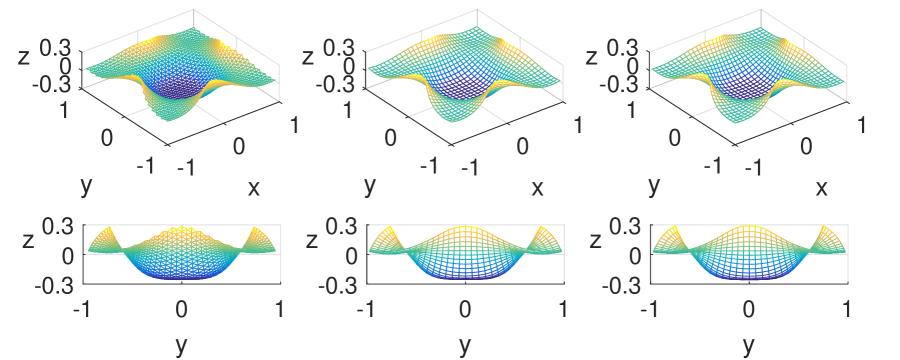
Figure 3: Static equilibria for the triangular lattice algorithm (left), and the finite difference algorithms with different Poisson ratios in one of the bending energy terms (center and right). The reference metrics are given by $\eta=\eta_{1}$ in (34), with physical parameters $A=0.1$, $k=1$, $h=0.03$, $\mu=1000$, and $\nu=1/3$ or $-1/3$ in certain bending energy terms (see text).

We now present a sequence of simulation results to display basic aspects of the algorithms and parameters. First, we compare the triangular lattice and finite difference methods in two situations. The first is the equilibrium sheet deformation with a nontrivial, but static (time-independent) reference metric given by $\eta=\eta_{1}$ in (34), with $A=0.1$, $k=1$, $h=0.03$, $\mu=1000$, and $\nu=1/3$. The sheets are initially nearly flat squares ($z=0.02(x_{1}^{4}+x_{2}^{4})$, $-1\leq x_{1}=x,x_{2}=y\leq 1$), and rapidly buckle into the shapes shown in figure 3. Three sheets are shown in oblique view (top row) and side view (bottom row). The leftmost sheet is computed with the triangular lattice algorithm, with jagged edges along one pair of sides. The center sheet is the result of the finite difference algorithm, with a different Poisson ratio value in one of the bending energy terms, to match those of the triangular lattice algorithm. For equilibrium metrics (37) we may write (12) as

$$w_{b}=\frac{Eh^{3}}{24(1-\nu^{2})}\eta^{4}\left((b_{11}+b_{22})^{2}-2(1-\nu)(b_{11}b_{22}-b_{12}^{2})\right).$$ (46)

In the stretching energy term (11) and the prefactor of the right hand side of (46), we set $\nu=1/3$, but we set $\nu$ to -1/3 in the second appearance of $\nu$ (within $1-\nu$) on the right hand side of (46). This gives an elastic energy consistent with that of the triangular lattice model schmidt2012universal . The rightmost sheet is also given by the finite difference algorithm but with $\nu=1/3$ in all stretching and bending energy terms. The deformations are very close in all three cases. The differences between maximum and minimum $z$ values, $\Delta z$, are within 1% for the center and leftmost sheets, and the difference is about 2% for the center and rightmost sheets. In this case at least, the error in Gaussian bending rigidity in the triangular lattice algorithm has a modest effect, as was found by didonna2002scaling in a different problem.

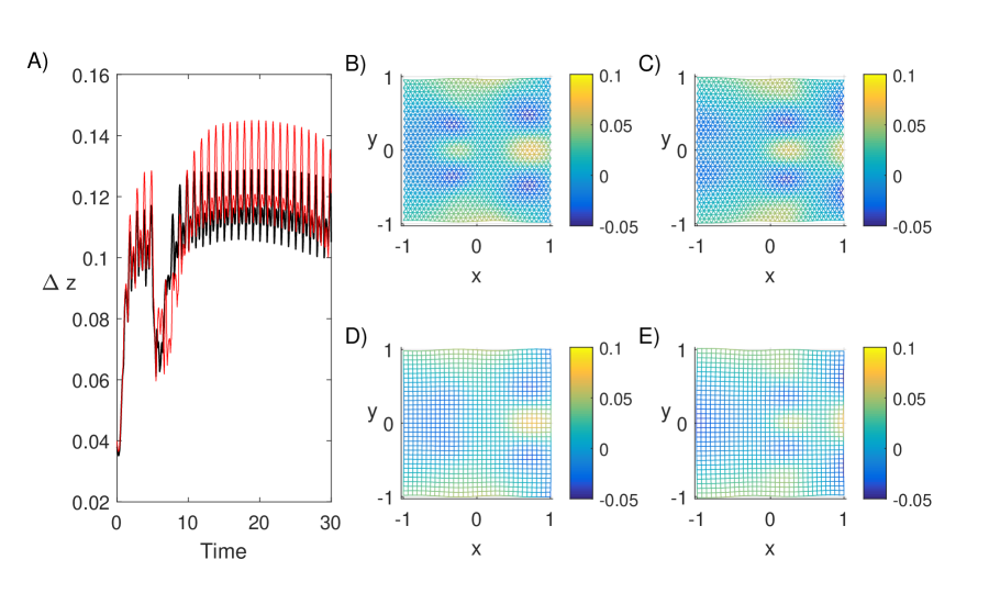
Figure 4: A comparison of sheet dynamics with the triangular lattice and finite difference algorithms with reference metric factor $\eta=\eta_{2}$ in (35), a unidirectional traveling wave, starting from a nearly flat sheet. The physical parameters are $A=0.03$, $k=1$, $h=0.03$, $\mu=1000$, and $\nu=1/3$. A) A comparison of the $z$-deflection over time for the triangular lattice (black) and finite difference (red) algorithms. Distributions of $z$ deflection at time $t$ = 29.5 and 30 are shown in panels B and C for the triangular lattice and D and E for the finite difference method, respectively.

We now consider an unsteady reference metric, $\eta=\eta_{2}$ in (35), a unidirectional traveling wave, in both algorithms. We again take square sheets, with the same spatial grids and initial conditions as before, with (smaller) $A=0.03$, $k=1$, $h=0.03$, $\mu=1000$, and $\nu=1/3$ (in all energy terms in both algorithms now, for simplicity). The time step $\Delta t=0.005$. Figure 4 compares the dynamics. Panel A shows $\Delta z$ versus time for the triangular lattice (black) and finite difference (red) algorithms. The dynamics after buckling of the initial state are quite complex, and include the appearance of a higher buckling mode during $6\leq t\leq 8$. For both algorithms the solutions have a strong oscillatory component with the same frequency as the reference metric, as one would expect. The solutions have other components that evolve on much longer time scales (tens to hundreds of periods), and even with modest deflections (here, about 7% of the square side length), the solutions can evolve in complicated ways over long time scales. The two algorithms show rough qualitative agreement, though the discrepancy in deflection reaches 10–15% at certain times in panel A. The $z$ deflection at $t$ = 29.5 and 30 is shown in panels B and C for the triangular lattice and D and E for the finite difference method, respectively. Both algorithms show a similar distribution of deflection on the right side of the sheets. On the left side, the triangular lattice has an additional peak (near $x=-0.25,y=0$) that is not present in the finite difference method.

We have illustrated the behavior of the algorithms in two simple cases. We’ve seen close agreement in the final equilibrium after buckling with a steady reference metric, and somewhat less agreement in a dynamical problem with a unidirectional traveling wave metric. The disagreements may be attributed to the sensitivity of the dynamical problem to different prefactors in the Gaussian curvature term of the bending energy and to the different spatial discretizations. We now proceed to illustrate some other basic features of the buckling behavior and dynamics, with the triangular lattice approach only for brevity.

Figure 5: Change in out-of-plane deflection from $t=0$ to $t=2$ for a unit hexagon with a small initial deflection $z=10^{-8}x_{1}x_{2}$, and imposed reference metric (34) with $k$ = 1, varying metric factor amplitude $A$ (horizontal axis) and varying sheet thickness $h$ (vertical axis). The damping constant $\mu=12.6$ and the mesh spacing $d$ = 1/33. The solid red line shows the locus of zero change in deflection, essentially the “buckling threshold.” The red crosses show, at several values of $h$, the values of $A$ on the buckling threshold with a finer mesh spacing, 1/66. The white line shows the scaling $A\sim h^{2}$.

If a static reference metric cannot be realized by a surface in $\mathbb{R}^{3}$, the sheet has nonzero stretching energy, and in general becomes unstable to out-of-plane buckling for sufficiently small $h$ efrati:2009b . Intuitively, buckling allows a reduction in stretching energy at the expense of bending energy. The relative cost of bending decreases with decreasing $h$, making buckling more favorable. For the static metric with $\eta=\eta_{1}$ in (34), we plot a computational estimate of the “buckling threshold”—for various $A\in[10^{-5},10^{-1}]$, the values of $h$ at which buckling occurs. Here buckling is defined by whether a small initial deflection ($z=10^{-8}x_{1}x_{2}$) grows after two time units, with a certain damping constant ($\mu=12.6$). Changes in the time interval and damping constant have only a slight effect on the buckling threshold, plotted as a red solid line for $d=1/33$. The mesh spacing becomes more important at smaller $h$, where buckling deformations may occur with a smaller wavelength due to the decreased bending energy. To check the effect of mesh refinement, we repeat the computations with $d=1/66$ at selected points and obtain the red crosses. The white line shows the scaling $A\sim h^{2}$, which approximately matches the buckling threshold data presented in efrati:2009b for a different reference metric. Our data appear to follow this trend for $h\geq 0.01$. Deviations at smaller $h$ are likely due to the finite mesh spacing.

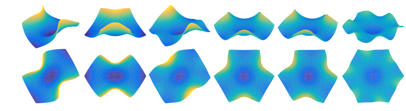
Figure 6: A selection of six buckled equilibria of the unit hexagon. Each is shown in two views: the top row gives views from 60 degrees with respect to the $z$-axis, and the bottom row gives views along the $z$-axis. The sheet thickness is $h=0.03$ and the imposed reference metric factor is $\eta=\eta_{1}$ given in (34) with $A=0.1$ and $k=1$. The equilibria are obtained by starting from different initial perturbations, with lattice spacing $d$ = 1/33.

Next, we study the postbuckling behavior, again with the static metric factor $\eta=\eta_{1}$ in (34) but with $A=0.1$, $k=1$, and different initial perturbations of the form $z=cr^{m}\sin(m\phi)$, where $r$ is the initial distance of sheet points from the hexagon center, $\phi$ is the azimuthal angle (with respect to the hexagon center), and $m$ is the azimuthal wavenumber, an integer from 2 to 6. The amplitude $c$ ranges from 0 to 0.1, and $\mu$ ranges from 1 to 1000. We obtain buckling into various equilibria akin to those studied by efrati:2009b with other radially symmetric reference metrics. We show six equilibria in figure 6, in two views (top and bottom rows). The first three (starting at the left) have a twofold azimuthal rotational symmetry, but are distinct configurations. The second has an additional bilateral symmetry and the third has an additional pair of local maxima along the sheet edges. The fourth and fifth have a threefold rotational symmetry, and the fourth has bilateral symmetries in addition. The sixth has a sixfold rotational symmetry. These are only a selection of local equilibria for a given static reference metric, and illustrate the complexity of the energy landscape for such sheets, even without dynamics and/or a time-dependent reference metric.

VI.1 Parameter sweeps

We next study the effects of parameters on the sheet dynamics, using the reference metric factor $\eta=\eta_{3}$ in (36), a radial traveling wave. We perform a sequence of parameter sweeps, varying one of $A$, $h$, or $\mu$ while keeping the others fixed. We fix the wavenumber $k$ at 1 in all cases. If $k$ is much smaller, the sheet does not buckle because the reference metric is almost uniform, and planar dilation/contraction is preferred energetically. If $k$ is much larger, buckling is also inhibited because the reference metric averaged over a local region approaches the identity tensor. As a base case, we take $A$ = 0.1, $\mu=1000$, and $h$ = 0.03, and vary each physical parameter in turn with numerical parameters $d=1/33$ and $\Delta t=0.005$. We initialize the sheet with a small out-of-plane deflection ($z=0.02(x_{1}^{4}+x_{2}^{4})$, $-1\leq x_{1}=x,x_{2}=y\leq 1$).

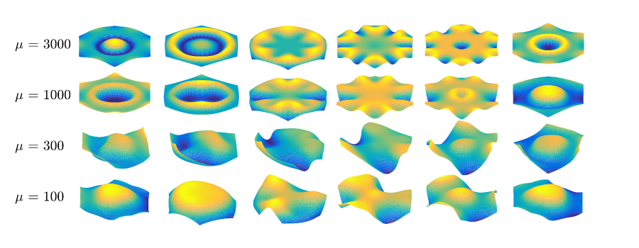
Figure 7: Snapshots of a unit hexagon, from $t$ = 19 to 20 in time increments of 0.2 (from left to right) with different damping constants $\mu$ (top to bottom), metric factor amplitude $A$ = 0.1 in (36) and $h$ = 0.03. The colors show the $z$ coordinate value, and the color scale is scaled to the minimum and maximum $z$ coordinate value of each sheet.

In figure 7 we show snapshots of a unit hexagon from $t$ = 19 to 20 in time increments of 0.2 (from left to right), for four different values of $\mu$, with $A$ = 0.1 and $h$ = 0.03. When $\mu$ is large, the sheet responds more slowly to the reference metric. The tendency is to oscillate about a mean state of no deformation (because the long-time-average reference metric is the identity tensor), and at sufficiently large $\mu$ the sheet does not buckle out of plane. At the largest $\mu$ (3000), the dynamics are essentially periodic (with period 2, so only a half-period is shown; the position at time $t+1$ is that at time $t$ but reflected in the $z=0$ plane). The out-of-plane deflection is smaller and more symmetric that at smaller $\mu$, where the dynamics become more chaotic and asymmetric. At smaller $\mu$, the sheet moves more rapidly through the complicated, time-dependent elastic energy landscape. At $\mu=1000$, the sheet deflection $\Delta z(t)$ has a large component with the same period as the reference metric, but also large components that are not periodic. At $\mu=300$, bilateral symmetry is lost, while at $\mu=100$, the sheet almost assumes a threefold symmetry.

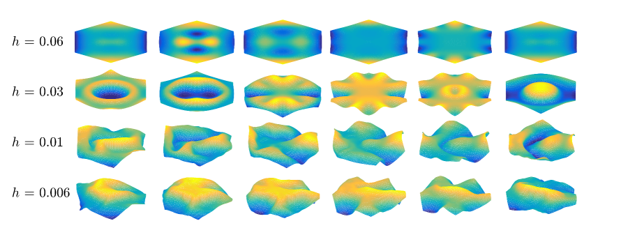
Figure 8: Snapshots of sheet dynamics with various sheet thicknesses $h$ (top to bottom), from $t$ = 19 to 20 in time increments of 0.2 (from left to right). Here $A$ = 0.1 and $\mu=1000$.

Next, we vary $h$, with $A$ = 0.1 and $\mu=1000$. Snapshots are shown in figure 8. With larger $h$, bending is relatively more costly, so the deformation is smoother, and at sufficiently large $h$ the sheet relaxes back to a planar state ($h=0.06$). At smaller $h$, the sheet motion is more chaotic and asymmetric, as for decreasing $\mu$. Notably, at smaller $h$ fine wrinkling features appear, and the deformation is far from any kind of symmetry. Eventually the sheet may intersect itself (not shown) because forces due to self-contact are not included.

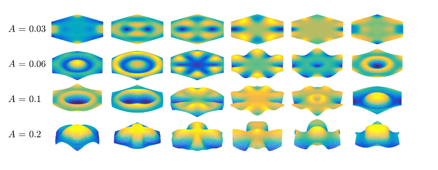
Figure 9: Snapshots of sheet dynamics with various metric factor amplitudes $A$ (in (36)), from $t$ = 19 to 20 in time increments of 0.2 (from left to right). Here $h$ = 0.03 and $\mu=1000$.

We vary $A$ next, with $h=0.03$ and $\mu=1000$. Here (figure 9) there is a sequence of dynamics from slow relaxation to planar motions ($A$ = 0.03), to periodic and symmetric ($A$ = 0.06, with period 2), to aperiodic but still bilaterally symmetric ($A$ = 0.1 and 0.2). At larger $A$ the deflection amplitude increases but the deformation remains relatively smooth, and in this sense the dynamics are more similar to smaller $\mu$ than to smaller $h$.

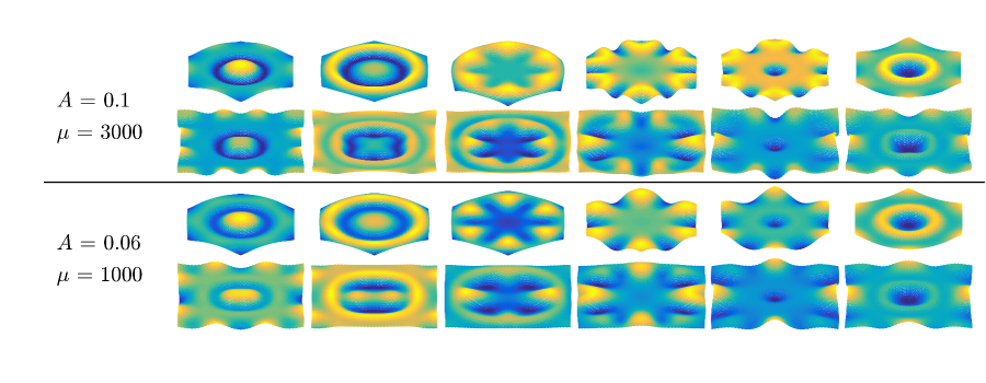
Figure 10: Comparisons of the dynamics of hexagonal and square sheets with $A=0.1$ and $\mu=3000$ in the top two rows and $A=0.06$ and $\mu=1000$ in the bottom two rows. All other parameters and initial conditions are the same as in figures 7 and 9 (e.g. $h=0.03$), and the snapshots run from $t$ = 19 to 20 in time increments of 0.2 (from left to right).

Finally, we consider the effect of the sheet shape on the dynamics. We consider the two cases with periodic dynamics above, ($A=0.1$, $\mu=3000$) in figure 7 and ($A=0.06$, $\mu=1000$) in figure 9, both with $h=0.03$. In the top two rows of figure 10, we compare the hexagonal sheet snapshots with those of a square sheet with the same parameters. Both sheets have width 2 when the reference metric is the identity. The bottom two rows make the same comparison with $A=0.06$ and $\mu=1000$. At each time, the hexagonal and square sheets have qualitative similarities. At the first time (leftmost snapshots), the sheets have a central hump. At the second time, an upward ring (yellow) appears. Third, the ring breaks up into an array of humps with sixfold symmetry for the hexagons, and either six- or fourfold symmetry for the squares. Fourth, the humps reach the sheet boundary. Fifth, a central depression forms, and sixth, it widens and is surrounded by an upward ring. The main differences between the squares and hexagons are that the squares more often have a fourfold rather than sixfold symmetry, the maximum deflections of the squares are larger, and the squares have a significant nonperiodic component in the dynamics. The comparison illustrates that periodic dynamics can be somewhat sensitive to sheet shape, which is perhaps not surprising given that chaotic dynamics are common and small changes in various parameters can shift periodic dynamics to chaotic dynamics.

VII Conclusion

We have presented semi-implicit algorithms that can simulate the dynamics of thin elastic sheets with large time steps. We focus on the case of elastic sheets with nontrivial steady or time-varying reference metrics in overdamped dynamics, but the methods should apply to other problems with internal or external forcing. The first algorithm simulates a triangular lattice mesh, and uses a splitting of the stretching force that has been used previously for computer graphics simulations of hair and cloth desbrun1999interactive ; selle2008mass . The semi-implicit bending force uses a biharmonic operator with free-edge boundary conditions. The algorithm appears to be unconditionally stable for a periodic reference metric. The second algorithm simulates a rectangular grid with finite-difference derivatives of the energy, and allows for general values of the Poisson ratio (and unlike the triangular lattice, a consistent value in all terms of the bending and stretching energies). The semi-implicit finite difference algorithm is analogous to that for the triangular lattice, involving a stretching force operator for zero-rest-length springs, and the biharmonic operator for an approximate bending force. The finite difference algorithm is not unconditionally stable, but typically has a maximum stable time step two to three orders of magnitude greater than that of an explicit scheme.

The two algorithms agree very closely for the deformation of a square sheet under a static reference metric, even allowing a different Poisson ratio ($-1/3$ instead of 1/3) in one of the bending energy terms. There is more disagreement in the deflection amplitude and pattern for a unidirectional traveling wave reference metric, but the dynamics are qualitatively similar. For the triangular lattice, we see phenomena similar to those reported previously with different radially-symmetric reference metrics efrati:2009b : a 1/2-power-law scaling of the buckling threshold in the space of sheet thickness and reference metric factor amplitude, and the presence of multiple stable equilibria with varying types of azimuthal and bilateral symmetry. For the case of a radial traveling wave reference metric, we showed some of the basic effects of sheet and metric parameters. In general, as the metric factor amplitude increases, the sheet thickness decreases, or the damping parameter decreases, the sheet moves from flat, periodic oscillations, to buckled periodic oscillations with various types of symmetries, to buckled motions with a combination of periodic and nonperiodic components, and varying degrees of symmetry/asymmetry. Below a critical sheet thickness, the motions have little semblance of symmetry or periodicity.

Appendix A Bending force

We denote the discrete biharmonic operator on the triangular mesh with free-edge boundary conditions as $\tilde{\Delta}^{2}_{x_{1},x_{2}}$, and because it is independent of the sheet configuration we may derive it for a sheet that is a portion of a flat triangular lattice with edge length $d$. $\tilde{\Delta}^{2}_{x_{1},x_{2}}$ is a mapping from (small) out-of-plane displacements at each point to the bending force at that point. The mapping is a sum of the force-displacement mappings for each pair of adjacent equilateral triangles, because the bending energy is also a sum over such units. For the four vertices in a given pair of neighboring triangles, a unit upward displacement of one of the two outer vertices (those not on the shared edge) yields a downward bending force at each of the outer vertices, equal by symmetry, and an upward force at each of the inner two vertices (those on the shared edge), equal and opposite to those at the outer vertices, to main net force and torque balance. The forces are proportional to the displacement by a constant that gives the desired bending modulus of the sheet. The bottom row of figure 2 shows examples of the stencils for this biharmonic operator at a few mesh points: an interior point (analogous to the 13-point biharmonic stencil on a rectangular mesh), a next-to-boundary point, and a boundary point. The discrete biharmonic operator $\tilde{\Delta}^{2}_{x_{1},x_{2}}$ has these stencil values multiplied by the triangle altitudes raised to the $-4$ power $\left(\sqrt{3}d/2\right)^{-4}$, while the linearized bending force operator has instead the same stencil values multiplied by $\left(\sqrt{3}d/2\right)^{-2}$ because the bending force is the gradient of the bending energy, which is approximately the biharmonic of the deflection multiplied by the sheet area per vertex.

References

- [1] C. R. Calladine. Theory of shell structures. Cambridge University Press, 1983.
- [2] L. B. Freund and S. Suresh. Thin film materials: stress, defect formation and surface evolution. Cambridge University Press, Cambridge, 2004.
- [3] Shahaf Armon, Efi Efrati, Raz Kupferman, and Eran Sharon. Geometry and Mechanics in the Opening of Chiral Seed Pods. Science, 333(6050):1726–1730, 2011.
- [4] B Audoly and A Boudaoud. Self-similar structures near boundaries in strained systems. Physical Review Letters, 91(8), 2003.
- [5] C. D. Santangelo. Buckling thin disks and ribbons with non-Euclidean metrics. Europhysics Letters, 86(3), 2009.
- [6] John A. Gemmer and Shankar C. Venkataramani. Shape selection in non-Euclidean plates. Physica D, 240(19):1536–1552, 2011.
- [7] Eran Sharon. Swell Approaches for Changing Polymer Shapes. Science, 335(6073):1179–1180, 2012.
- [8] Eran Sharon and Hillel Aharoni. Frustrated shapes. Nature Materials, 15(7):707–709, 2016.
- [9] E. Efrati, E. Sharon, and R. Kupferman. Elastic theory of unconstrained non-Euclidean plates. Journal of the Mechanics and Physics of Solids, 57(4):762–775, 2009.
- [10] Efi Efrati, Eran Sharon, and Raz Kupferman. The metric description of elasticity in residually stressed soft materials. Soft Matter, 9(34):8187–8197, 2013.
- [11] Jun-Hee Na, Arthur A. Evans, Jinhye Bae, Maria C. Chiappelli, Christian D. Santangelo, Robert J. Lang, Thomas C. Hull, and Ryan C. Hayward. Programming Reversibly Self-Folding Origami with Micropatterned Photo-Crosslinkable Polymer Trilayers. Advanced Materials, 27(1):79–85, 2015.
- [12] Yael Klein, Efi Efrati, and Eran Sharon. Shaping of elastic sheets by prescription of non-Euclidean metrics. Science, 315(5815):1116–1120, 2007.
- [13] Jungwook Kim, James A. Hanna, Myunghwan Byun, Christian D. Santangelo, and Ryan C. Hayward. Designing Responsive Buckled Surfaces by Halftone Gel Lithography. Science, 335(6073):1201–1205, 2012.
- [14] Zi Liang Wu, Michael Moshe, Jesse Greener, Heloise Therien-Aubin, Zhihong Nie, Eran Sharon, and Eugenia Kumacheva. Three-dimensional shape transformations of hydrogel sheets induced by small-scale modulation of internal stresses. Nature Communications, 4:1586, 2013.
- [15] T. H. Ware, M. E. McConney, J. J. Wie, V. P. Tondiglia, and T. J. White. Voxelated liquid crystal elastomers. Science, 347(6225):982–984, 2015.
- [16] Timothy J. White and Dirk J. Broer. Programmable and adaptive mechanics with liquid crystal polymer networks and elastomers. Nature Materials, 14(11):1087–1098, 2015.
- [17] A. Sydney Gladman, Elisabetta A. Matsumoto, Ralph G. Nuzzo, L. Mahadevan, and Jennifer A. Lewis. Biomimetic 4D printing. Nature Materials, 15(4):413, 2016.
- [18] Yen-Chih Lin, Ji-Ming Sun, Jen-Hao Hsiao, Yeukuang Hwu, C. L. Wang, and Tzay-Ming Hong. Spontaneous emergence of ordered phases in crumpled sheets. Phys. Rev. Lett., 103:263902, 2009.
- [19] B Roman and J Bico. Elasto-capillarity: deforming an elastic structure with a liquid droplet. Journal of Physics: Condensed Matter, 22(49):493101, 2010.
- [20] Hillel Aharoni and Eran Sharon. Direct observation of the temporal and spatial dynamics during crumpling. Nature Materials, 9(12):993–997, 2010.
- [21] Joseph D. Paulsen, Vincent Demery, K. Bugra Toga, Zhanlong Qiu, Thomas P. Russell, Benny Davidovitch, and Narayanan Menon. Geometry-Driven Folding of a Floating Annular Sheet. Physical Review Letters, 118(4), 27 2017.
- [22] R Yoshida, T Takahashi, T Yamaguchi, and H Ichijo. Self-oscillating gel. Journal of the American Chemical Society, 118(21):5134–5135, 1996.
- [23] Shingo Maeda, Yusuke Hara, Takamasa Sakai, Ryo Yoshida, and Shuji Hashimoto. Self-walking gel. Advanced Materials, 19(21):3480, 2007.
- [24] O Tabata, H Hirasawa, S Aoki, R Yoshida, and E Kokufuta. Ciliary motion actuator using self-oscillating gel. Sensors and Actuators A-Physical, 95(2-3):234–238, 2002.
- [25] O Tabata, H Kojima, T Kasatani, Y Isono, and R Yoshida. Chemo-mechanical actuator using self-oscillating gel for artificial cilia. In MEMS-03: IEEE The Sixteenth Annual International Conference on Micro Electro Mechanical Systems, Proceedings: IEEE Micro Electro Mechanical Systems, pages 12–15. IEEE, 2003.
- [26] Shingo Maeda, Yusuke Hara, Ryo Yoshida, and Shuji Hashimoto. Peristaltic motion of polymer gels. Angewandte Chemie-International Edition, 47(35):6690–6693, 2008.
- [27] Yusuke Shiraki and Ryo Yoshida. Autonomous Intestine-Like Motion of Tubular Self-Oscillating Gel. Angewandte Chemie-International Edition, 51(25):6112–6116, 2012.
- [28] VV Yashin and AC Balazs. Modeling polymer gels exhibiting self-oscillations due to the Belousov-Zhabotinsky reaction. Macromolecules, 39(6):2024–2026, 2006.
- [29] Olga Kuksenok, Victor V. Yashin, and Anna C. Balazs. Mechanically induced chemical oscillations and motion in responsive gels. Soft Matter, 3(9):1138–1144, 2007.
- [30] Victor V Yashin and Anna C Balazs. Theoretical and computational modeling of self-oscillating polymer gels. The Journal of chemical physics, 126(12):124707, 2007.
- [31] Olga Kuksenok, Debabrata Deb, Pratyush Dayal, and Anna C. Balazs. Modeling chemoresponsive polymer gels. Annual Review of Chemical and Biomolecular Engineering, 5(1):35–54, 2014. PMID: 24498954.
- [32] Mila Boncheva, Stefan A Andreev, L Mahadevan, Adam Winkleman, David R Reichman, Mara G Prentiss, Sue Whitesides, and George M Whitesides. Magnetic self-assembly of three-dimensional surfaces from planar sheets. Proceedings of the National Academy of Sciences, 102(11):3924–3929, 2005.
- [33] Silas Alben and Michael P Brenner. Self-assembly of flat sheets into closed surfaces. Physical Review E, 75(5):056113, 2007.
- [34] Silas Alben, Bavani Balakrisnan, and Elisabeth Smela. Edge effects determine the direction of bilayer bending. Nano Letters, 11(6):2280–2285, 2011.
- [35] Silas Alben. Bending of bilayers with general initial shapes. Advances in Computational Mathematics, 41(1):1–22, 2015.
- [36] Shravan K Veerapaneni, Abtin Rahimian, George Biros, and Denis Zorin. A fast algorithm for simulating vesicle flows in three dimensions. Journal of Computational Physics, 230(14):5610–5634, 2011.
- [37] HH Rosenbrock. Some general implicit processes for the numerical solution of differential equations. The Computer Journal, 5(4):329–330, 1963.
- [38] David Gottlieb and Steven A Orszag. Numerical analysis of spectral methods: theory and applications, volume 26. Siam, 1977.
- [39] Thomas Y Hou, John S Lowengrub, and Michael J Shelley. Removing the stiffness from interfacial flows with surface tension. Journal of Computational Physics, 114(2):312–338, 1994.
- [40] Mathieu Desbrun, Peter Schröder, and Alan Barr. Interactive animation of structured deformable objects. In Graphics Interface, volume 99, page 10, 1999.
- [41] Bernhard Eberhardt, Olaf Etzmuß, and Michael Hauth. Implicit-explicit schemes for fast animation with particle systems. In Computer Animation and Simulation 2000, pages 137–151. Springer, 2000.
- [42] Thomas Y Hou, John S Lowengrub, and Michael J Shelley. Boundary integral methods for multicomponent fluids and multiphase materials. Journal of Computational Physics, 169(2):302–362, 2001.
- [43] Andrew Selle, Michael Lentine, and Ronald Fedkiw. A mass spring model for hair simulation. In ACM Transactions on Graphics (TOG), volume 27, page 64. ACM, 2008.
- [44] Silas Alben. An implicit method for coupled flow–body dynamics. Journal of Computational Physics, 227(10):4912–4933, 2008.
- [45] Silas Alben. Simulating the dynamics of flexible bodies and vortex sheets. Journal of Computational Physics, 228(7):2587–2603, 2009.
- [46] Hsiao-Yu Chen, Arnav Sastry, Wim M van Rees, and Etienne Vouga. Physical simulation of environmentally induced thin shell deformation. ACM Transactions on Graphics (TOG), 37(4):146, 2018.
- [47] HS Seung and DR Nelson. Defects in flexible membranes with crystalline order. Phys. Rev. A, 38(2):1005 – 1018, 1988.
- [48] Warner Tjardus Koiter. On the nonlinear theory of thin elastic shells. Proc. Koninkl. Ned. Akad. van Wetenschappen, Series B, 69:1–54, 1966.
- [49] Philippe G Ciarlet. Un modèle bi-dimensionnel non linéaire de coque analogue à celui de wt koiter. Comptes Rendus de l’Académie des Sciences-Series I-Mathematics, 331(5):405–410, 2000.
- [50] Roman Vetter, Norbert Stoop, Thomas Jenni, Falk K Wittel, and Hans J Herrmann. Subdivision shell elements with anisotropic growth. International Journal for Numerical Methods in Engineering, 95(9):791–810, 2013.
- [51] Efi Efrati, Yael Klein, Hillel Aharoni, and Eran Sharon. Spontaneous buckling of elastic sheets with a prescribed non-Euclidean metric. Physica D, 235(1-2):29–32, 2007.
- [52] Jorge Nocedal and Stephen Wright. Numerical optimization. Springer Science & Business Media, 2006.
- [53] Ernst Hairer, Syvert P Norsett, and Gerhard Wanner. Solving Ordinary Differential Equations II: Stiff Problems. Springer, 1987.
- [54] Gerhard Gompper and Daniel M Kroll. Fluctuations of polymerized, fluid and hexatic membranes: continuum models and simulations. Current opinion in colloid & interface science, 2(4):373–381, 1997.
- [55] Alexander E Lobkovsky and TA Witten. Properties of ridges in elastic membranes. Physical Review E, 55(2):1577, 1997.
- [56] Jack Lidmar, Leonid Mirny, and David R Nelson. Virus shapes and buckling transitions in spherical shells. Physical Review E, 68(5):051910, 2003.
- [57] GA Vliegenthart and G Gompper. Forced crumpling of self-avoiding elastic sheets. Nature materials, 5(3):216, 2006.
- [58] Eleni Katifori, Silas Alben, Enrique Cerda, David R Nelson, and Jacques Dumais. Foldable structures and the natural design of pollen grains. Proceedings of the National Academy of Sciences, 107(17):7635–7639, 2010.
- [59] Etienne Couturier, J Dumais, E Cerda, and Elenei Katifori. Folding of an opened spherical shell. Soft Matter, 9(34):8359–8367, 2013.
- [60] Chloe M Funkhouser, Rastko Sknepnek, and Monica Olvera De La Cruz. Topological defects in the buckling of elastic membranes. Soft Matter, 9(1):60–68, 2013.
- [61] Duanduan Wan, David R Nelson, and Mark J Bowick. Thermal stiffening of clamped elastic ribbons. Physical Review B, 96(1):014106, 2017.
- [62] David R Nelson, Tsvi Piran, and Steven Weinberg. Statistical mechanics of membranes and surfaces. World Scientific, 2004.
- [63] Bernd Schmidt and Fernando Fraternali. Universal formulae for the limiting elastic energy of membrane networks. Journal of the Mechanics and Physics of Solids, 60(1):172–180, 2012.
- [64] Brian Anthony DiDonna. Scaling of the buckling transition of ridges in thin sheets. Physical Review E, 66(1):016601, 2002.
- [65] Joel L Weiner. On a problem of Chen, Willmore, et al. Indiana University Mathematics Journal, 27(1):19–35, 1978.
- [66] Efi Efrati, Eran Sharon, and Raz Kupferman. Buckling transition and boundary layer in non-Euclidean plates. Physical Review E, 80(1), 2009.