Symmetry Breaking Creates Electro-Momentum Coupling in Piezoelectric Metamaterials

Abstract

The momentum of deformable materials is coupled to their velocity. Here, we show that in piezoelectric composites which deform under electric fields, the momentum can also be coupled to the electric stimulus by a designed macroscopic property. To this end, we assemble these materials in a pattern with asymmetric microstructure, develop a theory to calculate the relations between the macroscopic fields, and propose a realizable system that exhibits this coupling. In addition to its fundamental importance, our design thus forms a metamaterial for mechanical wave control, as traversing waves are governed by the balance of momentum, and, in turn, the engineered electro-momentum coupling. While introduced for piezoelectric materials, our analysis immediately applies to piezomagnetic materials, owing to the mathematical equivalence between their governing equations, and we expect our framework to benefit other types of elastic media that respond to non-mechanical stimuli.

Keywords: dynamic homogenization, piezoelectric composite, Bloch Floquet waves, metamaterials, effective properties, constitutive relations, wave propagation, Willis coupling

Faculty of Mechanical Engineering, Technion–Israel Institute of Technology, Haifa 32000, Israel

1 Introduction

The effective or macroscopic properties of materials are modeled by the coupling parameters between physical fields in germane constitutive equations [1]; extraordinary properties are engineered by cleverly designing the microstructure of artificial materials. Such metamaterials were developed in optics, acoustics and mechanics for various objectives [2, 3, 4, 5].

One of the grand challenges in metamaterial design is to obtain control over traversing waves [6, 7, 8, 9, 10, 11, 12, 13, 14, 15, 16]. Mechanical waves are governed by the balance of momentum; at the microscale, the momentum is coupled only to the material point velocity by the mass density. Willis discovered that in elastic materials with a specific microstructure, the macroscopic momentum is coupled also to the strain by the now termed Willis coupling [17]. This coupling thus offers a designable degree of freedom to manipulate waves.

A series of theoretical studies were carried out to characterize Willis coupling and understand its physical origins [18, 19, 20, 21, 22, 23, 24, 25, 26]. Guided by accompanying predictions that Willis coupling is connected with unusual phenomena such as asymmetric reflections and unidirectional transmission, recent experimental realizations of Willis metamaterials that demonstrate these phenomena were reported [27, 28, 29, 30, 31, 32, 33, 34, 35]. To date, these investigations were limited to metamaterials that are deformable only by mechanical forces.

Here, we consider constituents that additionally deform by non-mechanical stimuli, namely, piezoelectric materials responding to electric fields [36, 37]. We construct asymmetric patterns of such responsive materials, and show that their macroscopic momentum can additionally be coupled by design to the stimulus. We call this macroscopic property the electro-momentum coupling (Fig. 1). Akin to the intrinsic piezoelectric and engineered Willis couplings, this coupling appears in (meta)materials with no inversion symmetry. Beyond its theoretical significance, mechanical metamaterials designed with this property can actively manipulate waves by modulation of the external stimulus, contrary to typical metamaterials whose functionality is fixed, cf. Refs.  [38, 39, 40, 41]. To this end, it is required to carry out complementary studies on the connection between the electro-momentum coupling, scattering properties, and medium composition [42], similarly to the process that was required in employing Willis coupling for metamaterial design [28, 25, 34]; the present work opens the route for these studies.

The macroscopic properties of metamaterials are analytically calculated using homogenization or effective medium theories [43, 44, 45, 46, 47, 48, 49, 50, 51, 52]. Guided by the effective elastodynamic theory of Willis [53, 54, 55, 56, 57, 58, 59], we develop a homogenization method for piezoelectric metamaterials, whose application unveils the electro-momentum coupling. Our method is based on three elements. Firstly, it employs a unified framework we developed to account for the microscopic interactions between the mechanical and non-mechanical fields. Secondly, it uses an averaging scheme whose resultant effective fields identically satisfy the macroscopic governing equations. To this end, we have adapted the ensemble averaging approach of Willis [57] to the current setting. Lastly, it incorporates driving forces that render the effective properties unique, as firstly advocated by Fietz and Shvets [44], and later in Refs. [57, 23].

Before proceeding, a short discussion on the applicability of Willis homogenization scheme, and by transitivity our scheme, is in order. First, we note that the scheme is independent of any assumptions, and delivers effective properties that identically satisfy the field equations and boundary conditions, therefore considered exact [18, 26]; in fact, asymptotic homogenization schemes were shown to be approximations of Willis homogenization [20, 26]. Thus, for infinite periodic medium, the scheme reproduces precisely the its corresponding band diagram. Still, for the homogenized fields to serve as good approximations of the microscopic ones, certain homogenizability conditions should be satisfied [18]. These show that beyond the long-wavelength low-frequency limit there is an additional range in which dynamic homogenization is meaningful [50]. We further note that the new coupling terms emerging from this scheme were found essential for obtaining an effective description that satisfies fundamental principles such as causality [23], similarly to the need for the analogous bianisotropic coupling in electromagnetics [60, 45].

The paper is structured as follows. In Sec. 2 we summarize the equations governing elastic waves in heterogeneous linearly responsive media, i.e., media that respond mechanically to non-mechanical loads. In Sec. 3 we develop our dynamic homogenization scheme for such media, and highlight the essential features of the resultant macroscopic properties. We apply our theory to longitudinal waves in piezoelectric layers assembled periodically with broken inversion symmetry in Sec. 4. A summary of our work concludes the paper in Sec. 5.

Before we proceed, we stress out that while this introduction was concerned with piezoelectric materials which respond to electric stimuli, our results immediately apply to piezomagnetic materials, owing to the mathematical similarity between their microscopic equations. We also expect our framework to benefit other types of elastic media that respond to non-mechanical stimuli, such as thermoelastic composites. These extensions are discussed in Appendix A

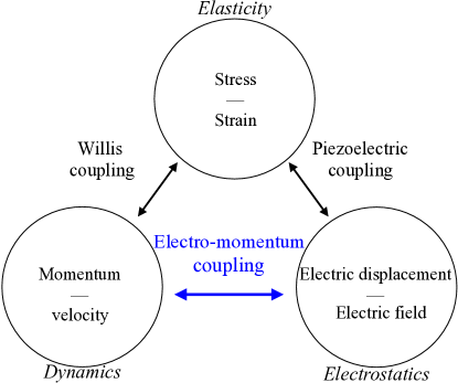
FIG. 1: Schematics of the electro-momentum coupling reported here, with respect to the intrinsic piezoelectric coupling and Willis metamaterial coupling. Similarly to piezoelectric and Willis couplings, the electro-momentum coupling appears in (meta)materials with no inversion symmetry. While the diagram refers to elasticity and electrostatics, it applies to other branches of physics: electrostatics is replaceable by magnetostatics, and elasticity by fluid mechanics.

2 Equations of piezoelectric composites

Consider a linear material with mass density $\rho$ and stiffness tensor $\mathbf{C}$ occupying the volume $\Omega$, subjected to prescribed body force density $\mathbf{f}$ and inelastic strain $\bm{\eta}$. Physically, $\bm{\eta}$ can result from a plastic process or phase transformation, where the mathematical motivation to account for it will be explained in the sequel [44, 57]. The response of the material is governed by the balance of linear momentum $\mathbf{p}$

$$\begin{aligned} \nabla\cdot\bm{\sigma}+\mathbf{f}-\dot{\mathbf{p}}=\mathbf{0},\end{aligned}$$ (1)

where $\bm{\sigma}$ is the Cauchy stress second-order tensor and the superposed dot denotes time derivative. The material mechanically interacts with the electric displacement $\mathbf{D}$, and electric field $\mathbf{E}$, which satisfy

$$\nabla\cdot\mathbf{D}=q,\quad\nabla\times\mathbf{E}=\mathbf{0},$$ (2)

where $q$ is a prescribed free charge density, acting as a source similarly to $\mathbf{f}$. Note that Eq. (2)₂ is identically satisfied by setting $\mathbf{E}=-\nabla\phi$.

The constitutive relations between the fields are written in symbolic matrix form [61]

$$\left(\begin{array}[]{c}\bm{\sigma}\\ \mathbf{D}\\ \mathbf{p}\end{array}\right)=\left(\begin{array}[]{ccc}\mathbf{C}&\mathbf{B}^{\mathsf{T}}&0\\ \mathbf{B}&-\mathbf{A}&0\\ 0&0&\rho\end{array}\right)\left(\begin{array}[]{c}\nabla\mathbf{u}-\bm{\eta}\\ \nabla\phi\\ \dot{\mathbf{u}}\end{array}\right),$$ (3)

where $\mathbf{u}$ is the displacement field, $\mathbf{A}$ and $\mathbf{B}$ are the dielectric and piezoelectric (tensorial) properties, and the transpose of $\mathbf{B}$ is defined by $B^{\mathsf{T}}_{ijk}=B_{kij}$. We assume the standard tensor symmetries, which in components read

$$A_{ij}=A_{ji},B_{ijk}=B_{jik},C_{ijkl}=C_{jikl}=C_{jilk}=C_{klij},\sigma_{ij}=\sigma_{ji}.$$ (4)

For later use, we denote the matrix (resp. column vector) in the right (resp. left) hand side of Eq. (3) by $\mathsf{L}$ (resp. $\mathsf{h}$).

We clarify that the elements in the symbolic matrices here and in what follows are differential operators and tensors of different order, and their product should be interpreted accordingly. For example, the product $\mathsf{L}_{11}\mathsf{m}_{1}$ represents double contraction, which in tensor notation is $\mathbf{C}:\bm{\eta}$, and in index notation is $C_{ijkl}\eta_{kl}$, while $\mathsf{L}_{12}\mathsf{b}_{2}$ is the single contraction $\mathbf{B}^{\mathsf{T}}\cdot\nabla\phi$, or $B^{\mathsf{T}}_{ijk}\phi_{,k}$. We further note that the symbolic matrix structure can be cast into standard matrix representation, using Voigt notation. Accordingly, $\mathbf{C},\mathbf{B}^{\mathsf{T}}$ and $\mathbf{B}$ are representable by $6\times 6,6\times 3$ and $3\times 6$ matrices, respectively, such that $\mathsf{L}$ is a symmetric $12\times 12$ matrix. (The zeros are $9\times 3$ and $3\times 9$ null matrices, and $\rho\mathbf{I}$ is a $3\times 3$ matrix.) The symmetric tensor $\bm{\sigma}$ is mapped to a $6\times 1$ column vector (and so is the symmetric part of $\nabla\mathbf{u}$), such that $\mathsf{h}$ is a $12\times 1$ column vector, and so on.

The prescribed boundary conditions are $\mathbf{u}=\mathbf{u}_{0}$ and $\phi=\phi_{0}$ over $\partial\Omega_{\mathsf{w}}\subset\partial\Omega$, and across the remaining boundary $\partial\Omega_{\mathsf{t}}=\partial\Omega\backslash\partial\Omega_{\mathsf{w}}$ are $\bm{\sigma}\cdot\mathbf{n}=\mathbf{t}_{0}$ and $\mathbf{D}\cdot\mathbf{n}=-w_{e}$, where $\mathbf{n}$ is the outward normal, $\mathbf{t}_{0}$ is the traction, and $w_{e}$ is the surface charge density.

When the medium is randomly heterogeneous, its properties $\rho,\mathbf{A},\mathbf{B}$ and $\mathbf{C}$ are functions of the position $\mathbf{x}$ and a parameter $y$ of a sample space $\Lambda$ with certain probability measure. Importantly, a periodic medium—the prevalent case of interest for metamaterials—can be analyzed as random, by considering different realizations of the composite generated by periodizing representative volume elements whose corner is a uniformly distributed random variable, and identifying $y$ with this variable. [57, 59].

Next, observe that ensemble averaging of Eqs. (1) and (2) over $y\in\Lambda$, denoted by $\left\langle\cdot\right\rangle$, provides

$$\begin{aligned} \nabla\cdot\left\langle\bm{\sigma}\right\rangle+\mathbf{f}-\dot{\left\langle\mathbf{p}\right\rangle}=\mathbf{0},\end{aligned}\quad\nabla\cdot\left\langle\mathbf{D}\right\rangle=q,$$ (5)

where $\left\langle\mathbf{f}\right\rangle=\mathbf{f}$ and $\left\langle q\right\rangle=q$ since $\mathbf{f}$ and $q$ are sure (prescribed). Eq. (5) suggests the use of $\left\langle\bm{\sigma}\right\rangle,\left\langle\mathbf{D}\right\rangle$ and $\left\langle\mathbf{p}\right\rangle$ as effective fields that identically satisfy the governing equations. The effective properties are thus the quantities that relate these effective fields with $\left\langle\nabla\mathbf{u}\right\rangle,\left\langle\dot{\mathbf{u}}\right\rangle$ and $\left\langle\nabla\phi\right\rangle$, to form effective constitutive relations. Together with Eq. (5), they establish a meaningful description of the material when the ensemble averaged fields fluctuate slowly enough relatively to the scale of the microstructure; for a rigorous description of the applicability conditions for homogenization see Ref. [18]. In periodic media undergoing Bloch-Floquet waves, these ensemble averages reduce to volume averages over the periodic part of each field [57, 18]. Qualitatively, the effective fields have the form of the curve in the right sketch of Fig. 2, after the fluctuations of the curve in the left sketch have been averaged out. The outstanding problem is to calculate the effective properties. Before we derive them, we can now provide a formal statement of our main result: homogenization shows that the effective constitutive relations are in the form

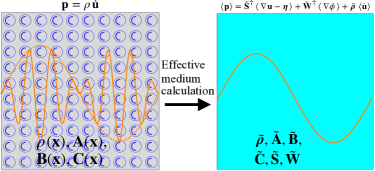
FIG. 2: Piezoelectric composite with asymmetric periodic cell, subjected to independent external sources. At the microscale, its momentum is $\mathbf{p}=\rho\dot{\mathbf{u}}$. Our effective medium theory reveals that the macroscopic momentum is $\left\langle\mathbf{p}\right\rangle=\tilde{\mathbf{S}}^{\dagger}\left\langle\nabla\mathbf{u}-\bm{\eta}\right\rangle+\tilde{\mathbf{W}}^{\dagger}\left\langle\nabla\phi\right\rangle+\tilde{\bm{\rho}}\left\langle\dot{\mathbf{u}}\right\rangle$.

$$\left(\begin{array}[]{c}\left\langle\bm{\sigma}\right\rangle\\ \left\langle\mathbf{D}\right\rangle\\ \left\langle\mathbf{p}\right\rangle\end{array}\right)=\left(\begin{array}[]{ccc}\tilde{\mathbf{C}}&\tilde{\mathbf{B}}^{\mathsf{T}}&\tilde{\mathbf{S}}\\ \tilde{\mathbf{B}}&-\tilde{\mathbf{A}}&\tilde{\mathbf{W}}\\ \tilde{\mathbf{S}}^{\dagger}&\tilde{\mathbf{W}}^{\dagger}&\tilde{\bm{\rho}}\end{array}\right)\left(\begin{array}[]{c}\left\langle\nabla\mathbf{u}\right\rangle-\bm{\eta}\\ \left\langle\nabla\phi\right\rangle\\ \left\langle\dot{\mathbf{u}}\right\rangle\end{array}\right),$$ (15)

with the electro-momentum coupling $\tilde{\mathbf{W}}^{\dagger}$ (Fig. 2), where $\left(\cdot\right)^{\dagger}$ denotes the adjoint operator with respect to the spatial variable. Thus, our homogenization process exposes effective couplings between $\left\langle\mathbf{D}\right\rangle$ and the average velocity, and between $\left\langle\nabla\phi\right\rangle$ and the average momentum. We denote the matrix of the effective properties in Eq. (15) by $\tilde{\mathsf{L}}$. The terms $\left\langle\nabla\mathbf{u}\right\rangle-\bm{\eta}$ and $\left\langle\dot{\mathbf{u}}\right\rangle$ that $\tilde{\mathsf{L}}$ operates on are independent, owing to $\bm{\eta}$, thus rendering $\tilde{\mathsf{L}}$ unique; otherwise, the fields $\left\langle\nabla\mathbf{u}\right\rangle$ and $\left\langle\dot{\mathbf{u}}\right\rangle$ are derived from the same potential, resulting with non-unique $\tilde{\mathsf{L}}$ [57], see, e.g., the example in Ref.  [62]. The calculation of $\tilde{\mathsf{L}}$ is detailed next.

3 Derivation of the effective properties

We adapt the ingenious approach of Willis [57] to responsive metamaterials as follows. Firstly, we cast the problem into matrix equations whose entries are tensors and other operators. Accordingly, Eqs. (1), (2)₁ and (3) take the form

$$\mathsf{D}^{\mathsf{T}}\mathsf{h}=-\mathsf{f},$$ (16)

$$\mathsf{h}=\mathsf{L}\left(\mathsf{b}-\mathsf{m}\right),$$ (17)

where

$$\begin{aligned} &\mathsf{B}=\left(\begin{array}[]{cc}\nabla&0\\ 0&\nabla\\ s&0\end{array}\right),\mathsf{m}=\left(\begin{array}[]{c}\bm{\eta}\\ 0\\ 0\end{array}\right),\mathsf{D}=\left(\begin{array}[]{cc}\nabla\cdot&0\\ 0&\nabla\cdot\\ -s&0\end{array}\right),\\ &\mathsf{w}=\left(\begin{array}[]{c}\mathbf{u}\\ \phi\end{array}\right),\mathsf{f}=\left(\begin{array}[]{c}\mathbf{f}\\ -q\end{array}\right),\mathsf{b}=\mathsf{B}\mathsf{w},\end{aligned}$$

and we employed the Laplace transform to replace time derivatives by products with $s$; to reduce notation, we retain the same symbols for the temporal and transformed fields, bearing in mind they now represent functions of $s$.

We define the Green’s function $\mathsf{G}\left(\mathbf{x},\mathbf{x}^{\prime}\right)$ via

$$\mathsf{D}^{\mathsf{T}}\mathsf{L}\mathsf{B}\mathsf{G}=-\left(\begin{array}[]{cc}\delta\left(\mathbf{x}-\mathbf{x}^{\prime}\right)\mathbf{I}&0\\ 0&\delta\left(\mathbf{x}-\mathbf{x}^{\prime}\right)\end{array}\right),$$ (18)

where $\mathbf{I}$ is the second order identity tensor and $\delta$ is the Dirac delta; the entries $\mathsf{G}_{11}$, $\mathsf{G}_{12}$ and $\mathsf{G}_{21}$, and $\mathsf{G}_{22}$ are second order tensor-, vector-, and scalar-valued functions, respectively, with the homogeneous boundary conditions

$$\mathsf{G}=0\ \mathrm{over}\ \partial\Omega_{\mathsf{w}},\quad\left(\mathsf{B}\mathsf{G}\right)^{\mathsf{T}}\mathsf{L}\mathsf{N}=0\ \mathrm{over}\ \partial\Omega_{\mathsf{t}},$$ (19)

where

$$\mathsf{N}^{\mathsf{T}}=\left(\begin{array}[]{ccc}\otimes\mathbf{n}&0&0\\ 0&\otimes\mathbf{n}&0\end{array}\right).$$

We derive next a useful expression for $\mathsf{w}$, by right multiplying the transpose of Eq. (18) by $\mathsf{w}\left(\mathbf{x}\right)$, subtracting it from the left product of Eq. (16) by $\mathsf{G}^{\mathsf{T}}\left(\mathbf{x},\mathbf{x}^{\prime}\right)$, and integrating the difference over the volume $\mathbf{x}^{\prime}\in\Omega$. The result is

$$\begin{aligned} \mathsf{w}(\mathbf{x},y)&=\int_{\Omega}\mathsf{G}^{\mathsf{T}}\mathsf{f}\mathrm{d}\Omega+\int_{\partial\Omega_{\mathsf{t}}}\mathsf{G}^{\mathsf{T}}\mathsf{N}^{\mathsf{T}}\mathsf{L}\left(\mathsf{B}\mathsf{w}-\mathsf{m}\right)\mathrm{d}a\\ &+\int_{\Omega}\left(\mathsf{B}\mathsf{G}\right)^{\mathsf{T}}\mathsf{L}\mathsf{m}\mathrm{d}\Omega-\int_{\partial\Omega_{\mathsf{w}}}\left(\mathsf{B}\mathsf{G}\right)^{\mathsf{T}}\mathsf{L}\mathsf{N}\mathsf{w}\mathrm{d}a,\end{aligned}$$ (20)

The development of Eq. (20) employs the divergence theorem, boundary conditions for $\mathsf{G}$ and symmetries of $\mathbf{A},\mathbf{B}$ and $\mathbf{C}$, and its detailed derivation using index and tensor notations is provided in Appendix B. Next, we manipulate the last integral in Eq. (20) as follows. First, we formally extend the integral domain from $\partial\Omega_{\mathsf{w}}$ to the whole boundary $\partial\Omega$ using the fact that the integrand vanishes over $\partial\Omega_{\mathsf{t}}$, owing to homogeneous boundary conditions that $\mathsf{G}$ satisfies over $\partial\Omega_{\mathsf{t}}$. Next, we can replace $\mathsf{w}$ with $\left\langle\mathsf{w}\right\rangle$, since it is sure on $\partial\Omega_{\mathsf{w}}$ and the integrand vanishes where it is not. By transforming the surface integral it back to the volume via the divergence theorem, and with the aid of Eq. (18), we can rewrite $\mathsf{w}$ as

$$\begin{aligned} \mathsf{w}(\mathbf{x},y)&=\int_{\Omega}\mathsf{G}^{\mathsf{T}}\mathsf{f}\mathrm{d}\Omega+\int_{\partial\Omega_{\mathsf{t}}}\mathsf{G}^{\mathsf{T}}\mathsf{N}^{\mathsf{T}}\mathsf{L}\left(\mathsf{B}\mathsf{w}-\mathsf{m}\right)\mathrm{d}a\\ &-\int_{\Omega}\left(\mathsf{B}\mathsf{G}\right)^{\mathsf{T}}\mathsf{L}\left(\left\langle\mathsf{B}\mathsf{w}\right\rangle-\mathsf{m}\right)\mathrm{d}\Omega+\left\langle\mathsf{w}\right\rangle.\end{aligned}$$ (21)

Using the ensemble average of Eq. (21) and the fact that $\mathsf{m},\mathsf{f},\mathbf{t}_{0}$ and $w_{e}$ are sure, we have that (see Appendix B for more details)

$$\mathsf{w}=\left\{\mathsf{G}^{\mathsf{T}}\left\langle\mathsf{G}\right\rangle^{-\mathsf{T}}\left\langle\left(\mathsf{B}\mathsf{G}\right)^{\mathsf{T}}\mathsf{L}\right\rangle-\left(\mathsf{B}\mathsf{G}\right)^{\mathsf{T}}\mathsf{L}\right\}\left(\left\langle\mathsf{B}\mathsf{w}\right\rangle-\mathsf{m}\right)+\left\langle\mathsf{w}\right\rangle.$$ (22)

Finally, we substitute Eq. (22) into Eq. (17) and ensemble average the result to obtain the effective constitutive relations

$$\left\langle\mathsf{h}\right\rangle\left(\mathbf{x}\right)=\tilde{\mathsf{L}}\left(\left\langle\mathsf{B}\mathsf{w}\right\rangle-\mathsf{m}\right),$$ (23)

with

$$\tilde{\mathsf{L}}=\left\langle\mathsf{L}\right\rangle-\left\langle\mathsf{L}\mathsf{B}\left(\mathsf{B}\mathsf{G}\right)^{\mathsf{T}}\mathsf{L}\right\rangle+\left\langle\mathsf{L}\mathsf{B}\mathsf{G}^{\mathsf{T}}\right\rangle\left\langle\mathsf{G}\right\rangle^{-\mathsf{T}}\left\langle\left(\mathsf{B}\mathsf{G}\right)^{\mathsf{T}}\mathsf{L}\right\rangle.$$ (24)

Eq. (24) generalizes the result of Willis [57] to metamaterials that interact with non-mechanical fields. The components of $\tilde{\mathsf{L}}$ define the effective properties in Eq. (15), which are non-local operators in space and time. The non-zero adjoint terms $\tilde{\mathsf{L}}_{23}$ and $\tilde{\mathsf{L}}_{32}$ reveal the coupling between $\left\langle\mathbf{D}\right\rangle$ and $\left\langle\dot{\mathbf{u}}\right\rangle$, and between $\left\langle\mathbf{p}\right\rangle$ and $\left\langle\nabla\phi\right\rangle$, respectively, denoted by $\tilde{\mathbf{W}}$. In the case that $\mathbf{D}$ and $\nabla\phi$ are vectors, the coupling $\tilde{\mathbf{W}}$ is a second order tensor. Owing to the symmetries of $\mathbf{A},\mathbf{B}$ and $\mathbf{C}$, the operator $\mathsf{L}$ is symmetric, so that $\mathsf{G}$ self-adjoint with the usual symmetries of Green functions, and hence $\tilde{\mathsf{L}}$ is self-adjoint as well, justifying the notation $\left(\cdot\right)^{\dagger}$ for $\tilde{\mathsf{L}}_{31}$ and $\tilde{\mathsf{L}}_{32}$.

4 Application to piezoelectric layers

We exemplify the emergence of the electro-momentum coupling by calculating the effective properties of an infinite repetition of commercially available piezoelectric layers. Specifically, we will study two different periodic cells, namely, (i) all-piezoelectric cell made of PZT4-BaTiO₃-PVDF layers, henceforth called composition 1, and (ii) one piezoelectric BaTiO₃ layer between elastic Al₂O₃ layer and another elastic PMMA layer, henceforth called composition 2. The material properties of the comprising phases are given in Tab. 1, where the values for the piezoelectric materials correspond to the coefficients in the direction of the poling.

Phase	$C\,\mathrm{(GPa})$	$\rho\,\mathrm{(kg/m^{3}})$	$B\,\mathrm{(C/m^{2}})$	$A$$(\textrm{nF/m})$
PZT4	$115$	7500	15.1	5.6
$\mathit{\textrm{BaTiO}_{\textrm{3}}}$	$165$	6020	3.64	0.97
PVDF	12	1780	-0.027	$0.067$
$\mathit{\textrm{Al}_{\mathrm{2}}}\textrm{O}_{3}$	300	3720	0	$0.079$
PMMA	3.3	1188	0	$0.023$

Table 1: Physical properties of the phases comprising the periodic piezoelectric laminate.

The periodic cell is denoted $\Omega_{\mathrm{p}}$, and its period is denoted $l$; in the calculations that follow we fix $l=3\,$mm. The layers are oriented such that the poling direction is along the direction of lamination, say $x$. The composite is driven by a body force density $f$ acting in the $x$ direction, along which axial inelastic strain $\eta$ is present; there are no free or surface charge sources in the problem ($w_{e}=q=0$). As a result, longitudinal waves propagate in the $x$ direction, such that the problem is one-dimensional and the pertinent fields can be treated as scalars. The objective is to obtain the macroscopic description of this problem by means of our homogenization scheme.

To this end, we analyze the periodic medium as random by treating the position of the period as a uniformly distributed random variable, with uniform probability density $l^{-1}$ over $\Omega_{\mathrm{p}}$. Accordingly, any $l$-periodic function $\zeta_{y}\left(x\right)$ in realization $y\in\Omega_{\mathrm{p}}$ is $\zeta_{0}\left(x-y\right)$; its ensemble average

$$\left\langle\zeta\right\rangle=\frac{1}{l}\int_{\Omega_{\mathrm{p}}}\zeta_{0}\left(x-y\right)\mathrm{d}y$$ (25)

is independent of $x$, and equals the spatial average in any realization.

We examine first the governing equations in realization $y=0$. In the absence of free charge, Gauss law within any layer reads

$$D_{0,x}^{\left(n\right)}=0,$$ (26)

where superscript $n=a,b$ and $c$ denotes values in the first, middle, and third layer, respectively. Note that $D$ is continuous across the layers, and since there are no electrodes and surface charge, we have that $D=0$ everywhere. Further, Eq.  (26) together with the constitutive relation

$$D_{0}^{\left(n\right)}=B_{0}^{\left(n\right)}u_{0,x}^{\left(n\right)}-A_{0}^{\left(n\right)}\text{$\phi_{0,x}^{\left(n\right)}$}$$ (27)

implies that

$$\text{$\phi_{0,xx}^{\left(n\right)}$}=\frac{B_{0}^{\left(n\right)}}{A_{0}^{\left(n\right)}}u_{0,xx}^{\left(n\right)}.$$ (28)

The second governing equation is the equation of motion, namely,

$$\sigma_{0,x}^{\left(n\right)}-s^{2}\rho_{0}^{\left(n\right)}u_{0}^{\left(n\right)}=-f_{0}^{\left(n\right)},$$ (29)

and we recall that the Laplace transform has been used, as in Sec.  3. Substituting in the constitutive relation for the stress

$$\sigma_{0}^{\left(n\right)}=C_{0}^{\left(n\right)}\left(u_{0,x}^{\left(n\right)}-\eta_{0}^{\left(n\right)}\right)+B_{0}^{\left(n\right)}\phi_{0,x}^{\left(n\right)}$$ (30)

and Eq.  (28) yields

$$\left(C_{0}+\dfrac{B_{0}^{2}}{A_{0}}\right)\left(u_{0,xx}-\eta_{,x}\right)-s^{2}\rho_{0}u_{0}=-f_{0},$$ (31)

where the superscript notation was suppressed for brevity. Since the homogeneous equation derived from Eq. (31) has periodic coefficients, its Green function is constructed using Bloch-Floquet solutions. The Green function and its ensemble average are thus

$$\begin{aligned} G_{0}\left(x,x^{\prime}\right)&=\left\{\begin{array}[]{l}Vu^{+}\left(x\right)u^{-}(x^{\prime}),\quad x<x^{\prime},\\[10.0pt] Vu^{+}(x^{\prime})u^{-}(x),\ \quad x^{\prime}<x,\end{array}\right.\\ \left\langle G\right\rangle\left(x,x^{\prime}\right)&=\frac{1}{l}\int_{\Omega_{\mathrm{p}}}G_{0}\left(x-y,x^{\prime}-y\right)\mathrm{d}y,\end{aligned}$$ (32)

where $\left\langle\mathsf{G}\right\rangle$ is only a function of $x-x^{\prime}$, $V$ is

$$V^{-1}=\left(C_{0}+\dfrac{B_{0}^{2}}{A_{0}}\right)\left(u^{+}_{,x}u^{-}-u^{+}u^{-}_{,x}\right),\ u^{\pm}=u_{\mathrm{p}}^{\pm}\left(x\right)e^{\pm ik_{B}x},$$ (33)

and $u_{\mathrm{p}}^{\pm}$ are $l$-periodic functions whose standard (and tedious) calculation is detailed in Appendix C.

As the simplicity of the problem enabled a solution via a single Green function, a simpler equivalent to Eq. (22) for $u$ follows, namely,

$$\begin{aligned} u\left(x,y\right)=&\left(G\left\langle G\right\rangle{}^{-1}\left\langle G_{,x^{\prime}}\check{C}\right\rangle-G{}_{,x^{\prime}}\check{C}\right)\left(\left\langle u_{,x^{\prime}}\right\rangle-\eta\right)\\ &+\left(G\left\langle G\right\rangle{}^{-1}\left\langle G\rho\right\rangle-G\rho\right)s^{2}\left\langle u\right\rangle+\left\langle u\right\rangle,\end{aligned}$$ (34)

where $\check{C}=C+\dfrac{B^{2}}{A}$. Observing that in the prescribed settings $D=0$ in any realization, we obtain the remaining fields $\phi\left(x,y\right)$ from Eq. (3) in terms of $u\left(x,y\right),A\left(x,y\right)$ and $B\left(x,y\right)$.

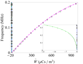
(a) $\xi l=0$

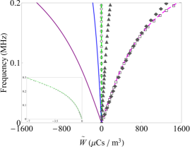
(b) $\xi l=2$

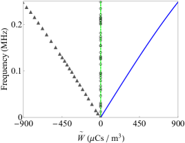
(c) $\xi l=2$, $l^{(b)}=0$

FIG. 3: Frequency versus $\tilde{W}$ and $\tilde{W^{\dagger}}$. Legend of composition 1 (resp. 2): Re$\,\tilde{W}$ in solid blue (purple) curves; Im$\,\tilde{W}$ in dashed green (pink) curves; Re$\,\tilde{W^{\dagger}}$ in triangle (diamond) marks; Im$\,\tilde{W^{\dagger}}$ in circle (square) marks. Panel (c) is for composition 1 with $l^{(b)}=0,l^{(a)}=l^{(c)}$, where $l^{(a)},l^{(b)}$ and $l^{(c)}$ denote the thickness of the first, middle and last layer of the unit cell, respectively.

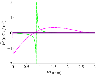
(a)

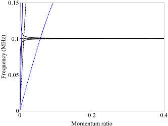
(b)

FIG. 4: (a) $\tilde{W}$ versus $l^{(b)}$ at 0.1 MHz and $\xi l=0$. (b) Frequency versus $\frac{\left|\tilde{W}^{\dagger}\left\langle\nabla\phi\right\rangle\right|}{\left|\tilde{\rho}\left\langle\dot{u}\right\rangle\right|}$ (solid curves) and $\frac{\left|\tilde{S}^{\dagger}\left\langle\nabla u\right\rangle\right|}{\left|\tilde{\rho}\left\langle\dot{u}\right\rangle\right|}$ (dotted curves) at $\xi l=0$. Black and blue curves correspond to compositions 1 (with $l^{(b)}=0.87\,$mm) and 2, respectively.

Finally, the equivalents of Eqs. (23)-(24) are derived directly by substituting $u\left(x,y\right)$ and $\phi\left(x,y\right)$ into Eq. (3), ensemble averaging, and identifying the terms that multiply $\left\langle u_{,x^{\prime}}\right\rangle-\eta,\left\langle\phi_{,x^{\prime}}\right\rangle$ and $\left\langle su\right\rangle$ as the effective properties according to Eq. (15). The price for using a single Green function in the absence of charge is one degree of freedom in calculating $\tilde{\mathsf{L}}$, which we eliminate by enforcing $\tilde{B}^{\mathsf{T}}=\tilde{B}$. Together with this choice, the resultant equations determine the components of $\tilde{\mathsf{L}}$. The explicit expressions are provided in Appendix D, and imply that

$$\begin{aligned} \tilde{S}\left(\xi\right)&=\tilde{S}^{\dagger}\left(-\xi\right)=-\mathrm{conj}\,\tilde{S}^{\dagger}\left(\xi\right)\\ \tilde{W}\left(\xi\right)&=\tilde{W}^{\dagger}\left(-\xi\right)=-\mathrm{conj}\,\tilde{W}^{\dagger}\left(\xi\right),\end{aligned}$$ (35)

where $\mathrm{conj}$ denotes complex conjugate, and $\xi$ is the Fourier transform variable, i.e.,

$$\tilde{\mathsf{L}}\left(\xi\right)=\int_{\Omega_{\mathrm{p}}}\tilde{\mathsf{L}}\left(x\right)e^{i\xi x}\mathrm{d}x.$$ (36)

These relations also imply that Re$\,\tilde{W}$ is an odd function of $\xi$, while Im$\,\tilde{W}$ is an even function, similarly to the functional form of $\tilde{S}$ [23]. Eq. (35) consolidates the notation used by Willis [56, 57, 58, 59], who interprets $\tilde{S}$ and $\tilde{S}^{\dagger}$ as formal adjoints with respect to the spatial variable, and other notations in the literature [63, 64, 23], which use $-\mathrm{conj}\,\tilde{S}$ instead of $\tilde{S}^{\dagger}$.

The numerical results in Fig. 3 display the Fourier transform $\tilde{W}\left(\xi\right)$ and its adjoint versus frequency $\frac{\omega}{2\pi}$, where $s=-i\omega$, across the first pass band. The calculations are done for the microstructure $l^{\left(a\right)}=1\,$mm (thickness of the first layer in the periodic cell) $,l^{\left(b\right)}=1.4\,$mm (middle layer), and $l^{\left(c\right)}=0.6\,$mm (last layer). Panel 3a shows the long-wavelength limit $\xi l=0$, which contains the homogenization limit [65, 50], where in Panel 3b we examine $\xi l=2$. For brevity, we omit the plots for the remaining effective properties, noting they are frequency-dependent, real at $\xi l=0$ (except $\tilde{S}$ and $\tilde{S}^{\dagger}$, which are pure imaginary), and generally complex for $\xi l>0$.

Evidently, the contrast between the piezoelectric coefficients of the layers greatly affects the magnitude of $\tilde{W}$. For example, the maximal value of Im$\,\tilde{W}$ at $\xi l=0$ for composition 1 is 21$\>\mu$Cs$\mathrm{m}^{-3}$, while for composition 2 it is over 900$\>\mu$Cs$\mathrm{m}^{-3}$.

Both compositions share the following notable features. Firstly, the electro-momentum coupling $\tilde{W}$ vanishes in the quasi-static limit $\omega\rightarrow 0$, as it should. In the long-wavelength limit and $\omega>0$, it attains non-zero pure imaginary values, as Eq. (35) implies. Above the long-wavelength limit, the numerical results confirm that the electro-momentum is complex such that Im$\tilde{\,W}=$Im$\,\tilde{W}^{\dagger}$ and Re$\tilde{\,W}=-$Re$\,\tilde{W}^{\dagger}$. Our observations conform with the insights of Sieck et al. [23] on the microstructure-induced Willis coupling: the imaginary part originates from broken inversion symmetry, hence appears even in the long-wavelength limit, while mesoscale effects of multiple scattering create its real part, hence appear at $\xi l>0$. This is further demonstrated in Panel  3c, where we evaluate $\tilde{W}$ and $\tilde{W}^{\dagger}$ at $\xi l=2$ in a system that is symmetric under inversion by setting $l^{\left(b\right)}=0$ in composition 1. Indeed, the coupling is pure real in this setting, and satisfies satisfies $\tilde{W}\left(\xi\right)=-\tilde{W}^{\dagger}\left(\xi\right)$.

Fig. 4a directly evaluates the dependency of $\tilde{W}$ on the microstructure, by plotting it against $l^{(b)}$ while setting $l^{(a)}=l^{(c)}$, at the representative frequency 0.1 MHz. The couplings vanish for $l^{(b)}=0$ and 3 mm, as it should for microstructures with inversion symmetry. Notably, the change from $l^{(b)}=0$ to $l^{(b)}=0^{+}$ is discontinuous for composition 2, as it reflects a shift from an elastic composition to a piezoelectric one. Interestingly, the coupling of composition 2 vanishes also at $l^{(b)}=0.79\,$mm, where the coupling of composition 1 exhibits singularity in the vicinity of $l^{(b)}=0.87\,$mm. These values are functions of the frequency; for example, at 0.05 MHz we calculated lower values, namely, $l^{(b)}=0.77\,$mm and $l^{(b)}=0.84\,$mm, respectively.

Lastly, in Fig. 4b we evaluate the frequency versus the momentum ratios between $\left|\tilde{W}^{\dagger}\left\langle\nabla\phi\right\rangle\right|,\left|\tilde{S}^{\dagger}\left\langle\nabla u\right\rangle\right|$ and $\left|\tilde{\rho}\left\langle\dot{u}\right\rangle\right|$ at $\xi l=0$, for composition 1 with $l^{(b)}=0.87\,$mm (black curves), and composition 2 (blue curves) with the microstructure studied in Fig. 3. Composition 1 exhibits a singularity at 1 MHz, conforming with the singularity observed in Fig. 4a. In the vicinity of 1 MHz, the growth of $\left|\tilde{W}^{\dagger}\left\langle\nabla\phi\right\rangle\right|$ is much faster than $\left|\tilde{S}^{\dagger}\left\langle\nabla u\right\rangle\right|$. Composition 2 demonstrates lower ratios, as expected from a metamaterial with an arbitrarily chosen microstructure.

5 Summary and discussion

We have developed an exact source-driven homogenization scheme for responsive metamaterials, based on the ensemble averaging approach of Willis and applied it in a numerical example considering periodic repetitions of commercially available piezoelectric layers. The scheme reveals that the effective non-mechanical and momentum-velocity fields can be coupled by properly designing the microstructure and composition of the medium. We conjecture that the corresponding couplings are necessary for obtaining an effective description that respect fundamental principles such as causality, similarly to the need for Willis coupling in elastodynamics [23] and bianisotropic coupling in electromagnetics [60, 45]. The new couplings reflect energy conversion between electrical and mechanical energy in a distinct way than it occurs at the microscale. Therefore, they capture a new mechanism that can be employed for rectifying mechanical waves by modulation of external stimuli. We expect that future studies will show that extraordinary wave response such as asymmetric reflections and unidirectional transmission are modeled by the new couplings [42], analogously to Willis coupling   [28, 32, 33, 34]. These kind of results are to be guided by theoretical analyses based upon proper homogenization schemes [25]. The present work opens the route for such studies on the properties of the electro-momentum coupling and its experimental realizations for metamaterial design.

Appendix A. Implications on other stimuli-responsive media

The structure we developed and its resultant effective description immediately apply for piezomagnetic media, by observing the following mathematical connections. The fields $\mathbf{D}$ and $\mathbf{E}$ are equivalent to the magnetic induction and magnetic field (usually denoted by $\mathbf{B}$ and $\mathbf{H}$, respectively), since they both satisfy identical differential equations. The latter two fields are constitutively related by the second-order permeability tensor (usually denoted by $\mu$), and their coupling with the stress and strain is captured by the piezomagnetic third-order tensor [66]. Thereby, homogenization of piezomagnetic composites fits exactly into our scheme, which predicts new macroscopic second-order tensors that couple the magnetic induction and the velocity, and the momentum and the magnetic field.

Implications of our scheme to thermoelasticity are less immediate and require a separate treatment. However, at the very basic level, we can draw analogies between $\mathbf{D}$ and the increase of entropy per unit volume with respect to a reference state (denoted $\vartheta$) , and between $\mathbf{E}$ and the change in temperature with respect to some base temperature (denoted $\theta$). The fields $\vartheta$ and $\theta$ are scalar fields that are constitutively coupled through the constant of specific heat. The microscopic cross-coupling between $\vartheta$ and $\theta$ to the stress and strain is captured by the thermal expansion second-order tensor, see Eq.  (2.24) in [66]. We now proceed to the differential equations that govern thermoelasticity. While $\mathbf{D}$ and $\mathbf{B}$ are subjected to the same differential equation, there is no such spatial constraint on $\vartheta$; in some approximated formulations of thermoelasticity, the equations of heat conduction and energy balance can be combined to form with the equation of motion two coupled field equations for the temperature and displacement, see Eqs.  (2.10-23) or Eqs.  (9.6-7)-(9.6-8) in [67]. We conjecture that homogenizing this system will expose new macroscopic couplings between $\vartheta$ and the velocity, and between the momentum and $\theta$.

Appendix B. Detailed derivation of $\tilde{\mathsf{L}}$ in index and tensor notation

Eq. (16) in tensor notation is

$$\left(\begin{array}[]{c}\nabla\cdot\bm{\sigma}-s^{2}\rho\mathbf{u}\\ \nabla\cdot\mathbf{D}\end{array}\right)+\left(\begin{array}[]{c}\mathbf{f}\\ -q\end{array}\right)=\left(\begin{array}[]{c}\mathbf{0}\\ 0\end{array}\right).$$ (B.1)

The left product of Eq. (B.1) with $\mathsf{G}^{\mathsf{T}}\text{$\left(\mathbf{x},\mathbf{x}^{\prime}\right)$}$ is

$$\left(\begin{array}[]{c}\mathbf{G}_{11}^{\mathsf{T}}\cdot\left(\nabla\cdot\bm{\sigma}\right)+\mathbf{G}_{21}\nabla\cdot\mathbf{D}\\ \mathbf{G}_{12}\cdot\left(\nabla\cdot\bm{\sigma}\right)+\mathsf{G}_{22}\nabla\cdot\mathbf{D}\end{array}\right)-\left(\begin{array}[]{c}s^{2}\rho\mathbf{G}_{11}^{\mathsf{T}}\cdot\mathbf{u}\\ s^{2}\rho\mathbf{G}_{12}\cdot\mathbf{u}\end{array}\right)+\left(\begin{array}[]{c}\mathbf{G}_{11}^{\mathsf{T}}\cdot\mathbf{f}-\mathbf{G}_{21}q\\ \mathbf{G}_{12}\cdot\mathbf{f}-G_{22}q\end{array}\right)=\left(\begin{array}[]{c}\mathbf{0}\\ 0\end{array}\right),$$ (B.2)

or, in index notation,

$$\left(\begin{array}[]{c}G_{11pj}^{\mathsf{T}}\sigma_{jk,k}+G_{21p}D_{k,k}\\ G_{12j}\sigma_{jk,k}+G_{22}D_{k,k}\end{array}\right)-\left(\begin{array}[]{c}s^{2}\rho G_{11pj}^{\mathsf{T}}u_{j}\\ s^{2}\rho G_{12j}u_{j}\end{array}\right)+\left(\begin{array}[]{c}G_{11pj}^{\mathsf{T}}f_{j}-G_{21p}\thinspace q\\ G_{12j}f_{j}-G_{22}\thinspace q\end{array}\right)=\left(\begin{array}[]{c}0_{p}\\ 0\end{array}\right).$$ (B.3)

The quantities $\mathsf{G}_{11}$, $\mathsf{G}_{12}$ and $\mathsf{G}_{21}$, and $\mathsf{G}_{22}$ are second order tensor-, vector-, and scalar-valued functions, respectively, and hence the symbolic $2\times 2$ matrix $\mathsf{G}$ is representable by a $4\times 4$ matrix. ($\mathsf{G}_{11}$, $\mathsf{G}_{12}$ and $\mathsf{G}_{21}$, and $\mathsf{G}_{22}$ are represented by $3\times 3,3\times 1,1\times 3$ and $1\times 1$ blocks, respectively.) The equation that defines $\mathsf{G}\left(\mathbf{x},\mathbf{x}^{\prime}\right)$ is

$$\mathsf{D}^{\mathsf{T}}\mathsf{L}\mathsf{B}\mathsf{G}=-\delta\mathsf{I},$$ (B.4)

where, in tensor notation, the elements of $\delta\mathsf{I}$ are

$$\delta\mathsf{I}=\left(\begin{array}[]{cc}\delta\left(\mathbf{x}-\mathbf{x}^{\prime}\right)\mathbf{I}&0\\ 0&\delta\left(\mathbf{x}-\mathbf{x}^{\prime}\right)\end{array}\right),$$

and the elements of $\mathsf{D}^{\mathsf{T}}\mathsf{L}\mathsf{B}\mathsf{G}$ are

$$\left(\begin{array}[]{cc}\nabla\cdot\left(\mathbf{C}:\nabla\mathbf{G}_{11}+\mathbf{B}^{\mathsf{T}}\cdot\nabla\mathbf{G}_{21}\right)-s^{2}\rho\mathbf{G}_{11}&\nabla\cdot\left(\mathbf{C}:\nabla\mathbf{G}_{12}+\mathbf{B}^{\mathsf{T}}\cdot\nabla G_{22}\right)-s^{2}\rho\mathbf{G}_{12}\\ \nabla\cdot\left(\mathbf{B}:\nabla\mathbf{G}_{11}-\mathbf{A}\cdot\nabla\mathbf{G}_{21}\right)&\nabla\cdot\left(\mathbf{B}:\nabla\mathbf{G}_{12}-\mathbf{A}\cdot\nabla G_{22}\right)\end{array}\right)$$ (B.7)

or, in index notation,

$$\left(\begin{array}[]{cc}\left\{C_{ijkl}G_{11kp,l}+B_{ijm}^{\mathsf{T}}G_{21p,m}\right\}{}_{,j}-s^{2}\rho G_{11ip}&\left\{C_{ijkl}G_{12k,l}+B_{ijk}^{\mathsf{T}}G_{22,k}\right\}{}_{,j}-s^{2}\rho G_{12i}\\ \left\{B_{jnm}G_{11np,m}-A_{jm}G_{21p,m}\right\}{}_{,j}&\left\{B_{ijk}G_{12j,k}-A_{ij}G_{22,j}\right\}{}_{,i}\end{array}\right).$$ (B.10)

We emphasize that the convention contraction is different when $\mathsf{G}$ is involved. For example, $\mathbf{C}:\nabla\mathbf{G}_{11}$ is $C_{ijkl}G_{11kp,l}$ and $\mathbf{B}^{\mathsf{T}}\cdot\nabla\mathbf{G}_{21}$ is $B_{ijm}^{\mathsf{T}}G_{21p,m}$. The standard convention (contraction with the first two indices of the right tensor) can be recovered observing that

$$C_{ijkl}G_{11kp,l}=G^{\mathsf{T}}_{11pk,l}C_{klij},$$

and thus $\mathbf{C}:\nabla\mathbf{G}_{11}=\nabla\mathbf{G}_{11}^{\mathsf{T}}:\mathbf{C}.$ Similarly,

$$B_{ijm}^{\mathsf{T}}G_{21p,m}=G_{21p,m}B_{mij},$$

and thus $\mathbf{B}^{\mathsf{T}}\cdot\nabla\mathbf{G}_{21}=\nabla\mathbf{G}_{21}\cdot\mathbf{B}$. Using such identities, the standard convention for divergence operation applies, i.e., acting on the last free index.

Right multiplying the transpose of Eq. (B.4) with $\mathsf{w}\left(\mathbf{x}\right)$ provides

$$\left(\begin{array}[]{c}\left\{G_{11pk,l}^{\mathsf{T}}C_{klij}+G_{21p,m}B_{mij}\right\}{}_{,j}u_{i}+\left\{G_{11pn,m}^{\mathsf{T}}B_{nmj}^{\mathsf{T}}-G_{21p,m}A_{mj}\right\}{}_{,j}\phi\\ \left\{C_{ijkl}G_{12k,l}+B_{ijk}^{\mathsf{T}}G_{22,k}\right\}{}_{,j}u_{i}+\left\{B_{ijk}G_{12j,k}-A_{ij}G_{22,j}\right\}{}_{,i}\thinspace\phi\end{array}\right)$$ (B.13)

$$-\left(\begin{array}[]{c}\rho s^{2}G_{11pi}^{\mathsf{T}}u_{i}\\ \rho s^{2}G_{12i}u_{i}\end{array}\right)=-\left(\begin{array}[]{c}\delta_{pi}u_{i}(\mathbf{x})\delta\left(\mathbf{x}-\mathbf{x}^{\prime}\right)\\ \phi(\mathbf{x})\delta\left(\mathbf{x}-\mathbf{x}^{\prime}\right)\end{array}\right).$$ (B.18)

Subtracting Eq. (B.18) from (B.3) yields

$$\left(\begin{array}[]{c}G_{11pj}^{\mathsf{T}}f_{j}-G_{21p}\thinspace q\\ G_{12j}f_{j}-G_{22}\thinspace q\end{array}\right)+\left(\begin{array}[]{c}G_{11pj}^{\mathsf{T}}\sigma_{jk,k}+G_{21p}D_{k,k}\\ G_{12j}\sigma_{jk,k}+G_{22}D_{k,k}\end{array}\right)-$$ (B.23)

$$\left(\begin{array}[]{c}\left\{G_{11pk,l}^{\mathsf{T}}C_{klij}+G_{21p,m}B_{mij}\right\}{}_{,j}u_{i}+\left\{G_{11pn,m}^{\mathsf{T}}B_{nmj}^{\mathsf{T}}-G_{21p,m}A_{mj}\right\}{}_{,j}\phi\\ \left\{C_{ijkl}G_{12k,l}+B_{ijk}^{\mathsf{T}}G_{22,k}\right\}{}_{,j}\thinspace u_{i}+\left(B_{ijk}G_{12j,k}-A_{ij}G_{22,j}\right){}_{,i}\phi\end{array}\right) =\left(\begin{array}[]{c}\delta_{pi}u_{i}(\mathbf{x})\delta\left(\mathbf{x}-\mathbf{x}^{\prime}\right)\\ \phi(\mathbf{x})\delta\left(\mathbf{x}-\mathbf{x}^{\prime}\right)\end{array}\right)$$ . (B.28)

Eq. (B.23) is simplified using the following relations

$$G_{11pj}^{\mathsf{T}}\sigma_{jk,k}+G_{21p}D_{k,k} = \left\{G_{11pj}^{\mathsf{T}}\sigma_{jk}\right\}{}_{,k}-G_{11pj,k}^{\mathsf{T}}\sigma_{jk}+\left\{G_{21p}D_{k}\right\}{}_{,k}-G_{21p,k}D_{k}$$

$$= \left\{G_{11pj}^{\mathsf{T}}\sigma_{jk}+G_{21p}D_{k}\right\}{}_{,k}-G_{11pj,k}^{\mathsf{T}}\left[C_{jkil}(u_{i,l}-\eta_{il})+B_{jki}^{\mathsf{T}}\phi_{,i}\right]$$

$$-G_{21p,k}\left[B_{kil}\left(u_{i,l}-\eta_{il}\right)-A_{ki}\phi_{,i}\right]$$

$$= \left\{G_{11pj}^{\mathsf{T}}\sigma_{jk}+G_{21p}D_{k}\right\}{}_{,k}-\left(G_{11pj,k}^{\mathsf{T}}C_{jkil}+G_{21p,k}B_{kil}\right)u_{i,l}$$

$$-\left(G_{11pj,k}^{\mathsf{T}}B_{jki}^{\mathsf{T}}-G_{21p,k}A_{ki}\right)\phi_{,i}+\left(G_{11pj,k}^{\mathsf{T}}C_{jkil}+G_{21p,k}B_{kil}\right)\eta_{il};$$

$$G_{12j}\sigma_{jk,k}+G_{22}D_{k,k} = \left\{G_{12j}\sigma_{jk}\right\}{}_{,k}-G_{12j,k}\sigma_{jk}+\left\{G_{22}D_{k}\right\}{}_{,k}-G_{22,k}D_{k}$$

$$= \left\{G_{12j}\sigma_{jk}+G_{22}D_{k}\right\}{}_{,k}-G_{12j,k}\left[C_{jkil}(u_{i,l}-\eta_{il})+B_{jki}^{\mathsf{T}}\phi_{,i}\right]$$

$$-G_{22,k}\left[B_{kil}\left(u_{i,l}-\eta_{il}\right)-A_{ki}\phi_{,i}\right]$$

$$= \left\{G_{12j}\sigma_{jk}+G_{22}D_{k}\right\}{}_{,k}-\left(C_{iljk}G_{12j,k}+B_{ilk}^{\mathsf{T}}G_{22,k}\right)u_{i,l}$$

$$-\left(B_{ijk}G_{12j,k}-A_{ik}G_{22,k}\right)\phi_{,i}+\left(G_{12j,k}C_{jkil}+G_{22,k}B_{kil}\right)\eta_{il};$$

$$\left\{G_{11pk,l}^{\mathsf{T}}C_{klij}+G_{21p,m}B_{mij}\right\}{}_{,j}u_{i} = \left\{\left(G_{11pk,l}^{\mathsf{T}}C_{klij}+G_{21p,m}B_{mij}\right)u_{i}\right\}{}_{,j}-\left(G_{11pk,l}^{\mathsf{T}}C_{klij}+G_{21p,m}B_{mij}\right)u_{i,j};$$

$$\left\{G_{11pn,m}^{\mathsf{T}}B_{nmj}^{\mathsf{T}}-G_{21p,m}A_{mj}\right\}{}_{,j}\phi = \left\{\left(G_{11pn,m}^{\mathsf{T}}B_{nmj}^{\mathsf{T}}-G_{21p,m}A_{mj}\right)\phi\right\}{}_{,j}-\left(G_{11pn,m}^{\mathsf{T}}B_{nmj}^{\mathsf{T}}-G_{21p,m}A_{mj}\right)\phi_{,j};$$

$$\left\{C_{ijkl}G_{12k,l}+B_{ijk}^{\mathsf{T}}G_{22,k}\right\}{}_{,j}u_{i} = \left\{\left(C_{ijkl}G_{12k,l}+B_{ijk}^{\mathsf{T}}G_{22,k}\right)u_{i}\right\}{}_{,j}-\left(C_{ijkl}G_{12k,l}+B_{ijk}^{\mathsf{T}}G_{22,k}\right)u_{i,j};$$

$$\left\{B_{ijk}G_{12j,k}-A_{ij}G_{22,j}\right\}{}_{,i}\phi = \left\{\left(B_{ijk}G_{12j,k}-A_{ij}G_{22,j}\right)\phi\right\}{}_{,i}-\left(B_{ijk}G_{12j,k}-A_{ij}G_{22,j}\right)\phi_{,i},$$

which, upon integration over the volume $\mathbf{x}\in\Omega$ and application of divergence theorem, then reads

$$\left(\begin{array}[]{c}u_{p}(\mathbf{x}^{\prime})\\ \phi(\mathbf{x}^{\prime})\end{array}\right) = \int_{\Omega}\left(\begin{array}[]{c}G_{11pj}^{\mathsf{T}}f_{j}-G_{21p}\thinspace q\\ G_{12j}f_{j}-G_{22}\thinspace q\end{array}\right)\mathrm{d}\Omega+\int_{\partial\Omega_{\mathsf{t}}}\left(\begin{array}[]{c}\left(G_{11pj}^{\mathsf{T}}\sigma_{jk}+G_{21p}D_{k}\right)n_{k}\\ \left(G_{12j}\sigma_{jk}+G_{22}D_{k}\right)n_{k}\end{array}\right)\mathrm{d}a$$ (B.35)

$$+ \int_{\Omega}\left(\begin{array}[]{c}\left(G_{11pj,k}^{\mathsf{T}}C_{jkil}+G_{21p,k}B_{kil}\right)\eta_{il}\\ \left(G_{12j,k}C_{jkil}+G_{22,k}B_{kil}\right)\eta_{il}\end{array}\right)\mathrm{d}\Omega$$ (B.38)

$$- \int_{\partial\Omega_{\mathsf{w}}}\left(\begin{array}[]{c}\left[\left(G_{11pk,l}^{\mathsf{T}}C_{klij}+G_{21p,m}B_{mij}\right)u_{i}\right]n_{j}+\left[\left(G_{11pn,m}^{\mathsf{T}}B_{nmj}^{\mathsf{T}}-G_{21p,m}A_{mj}\right)\phi\right]n_{j}\\ \left[\left(C_{ijkl}G_{12k,l}+B_{ijk}^{\mathsf{T}}G_{22,k}\right)u_{i}\right]n_{j}+\left[\left(B_{ijk}G_{12j,k}-A_{ij}G_{22,j}\right)\phi\right]n_{i}\end{array}\right)\mathrm{d}a,$$ (B.41)

or, in tensor notation,

$$\left(\begin{array}[]{c}\mathbf{u}(\mathbf{x}^{\prime})\\ \phi(\mathbf{x}^{\prime})\end{array}\right) = \int_{\Omega}\left(\begin{array}[]{c}\mathbf{G}_{11}^{\mathsf{T}}\cdot\mathbf{f}-\mathbf{G}_{21}q\\ \mathbf{G}_{12}\cdot\mathbf{f}-G_{22}q\end{array}\right)\mathrm{d}\Omega+\int_{\partial\Omega_{\mathsf{t}}}\left(\begin{array}[]{c}\mathbf{G}_{11}^{\mathsf{T}}\cdot\left(\bm{\sigma}\cdot\mathbf{n}\right)+\mathbf{G}_{21}\left(\mathbf{D}\cdot\mathbf{n}\right)\\ \mathbf{G}_{12}\cdot\left(\bm{\sigma}\cdot\mathbf{n}\right)+G_{22}\left(\mathbf{D}\cdot\mathbf{n}\right)\end{array}\right)\mathrm{d}a$$ (B.48)

$$+ \int_{\Omega}\left(\begin{array}[]{c}\left(\nabla\mathbf{G}_{11}^{\mathsf{T}}:\mathbf{C}+\nabla\mathbf{G}_{21}\cdot\mathbf{B}\right):\bm{\eta}\\ \left(\nabla\mathbf{G}_{12}:\mathbf{C}+\nabla G_{22}\cdot\mathbf{B}\right):\bm{\eta}\end{array}\right)\mathrm{d}\Omega$$ (B.51)

$$- \int_{\partial\Omega_{\mathsf{w}}}\left(\begin{array}[]{c}\left(\nabla\mathbf{G}_{11}^{\mathsf{T}}:\mathbf{C}+\nabla\mathbf{G}_{21}\cdot\mathbf{B}\right):\mathbf{u}\otimes\mathbf{n}+\left(\nabla\mathbf{G}_{11}^{\mathsf{T}}:\mathbf{B}^{\mathsf{T}}-\nabla\mathbf{G}_{21}\cdot\mathbf{A}\right)\cdot\phi\mathbf{n}\\ \left(\nabla\mathbf{G}_{12}:\mathbf{C}+\nabla G_{22}\cdot\mathbf{B}\right):\mathbf{u}\otimes\mathbf{n}+\left(\nabla\mathbf{G}_{12}:\mathbf{B}^{\mathsf{T}}-\nabla G_{22}\cdot\mathbf{A}\right)\cdot\phi\mathbf{n}\end{array}\right)\mathrm{d}a,$$ (B.54)

where the tensor product $\otimes$ between vectors $\mathbf{a}$ and $\mathbf{b}$ is defined by the action on a third vector $\mathbf{c}$, namely [68],

$$\left(\mathbf{a}\otimes\mathbf{b}\right)\cdot\mathbf{c}=\left(\mathbf{b}\cdot\mathbf{c}\right)\mathbf{a},$$

implying that $\left(\mathbf{a}\otimes\mathbf{b}\right)_{ij}=a_{i}b_{j}$ and $\left(\mathbf{T}\otimes\mathbf{b}\right)_{ijk}=T_{ij}b_{k}$ for second-order tensors $\mathbf{T}$. Accordingly,

$$\left(\mathbf{G}_{11}^{\mathsf{T}}\otimes\mathbf{n}\right):\bm{\sigma} =\mathbf{G}_{11}^{\mathsf{T}}\cdot\left(\bm{\sigma}\cdot\mathbf{n}\right),$$

$$\left(\mathbf{G}_{21}\otimes\mathbf{n}\right)\cdot\mathbf{D} =\mathbf{G}_{21}\left(\mathbf{D}\cdot\mathbf{n}\right),$$

$$\left(\mathbf{G}_{12}\otimes\mathbf{n}\right):\bm{\sigma} =\mathbf{G}_{12}\cdot\left(\bm{\sigma}\cdot\mathbf{n}\right),$$

$$\left(G_{22}\otimes\mathbf{n}\right)\cdot\mathbf{D} =G_{22}\left(\mathbf{D}\cdot\mathbf{n}\right),$$

which, by defining

$$\mathsf{N}^{\mathsf{T}}=\left(\begin{array}[]{ccc}\otimes\mathbf{n}&0&0\\ 0&\otimes\mathbf{n}&0\end{array}\right),$$

allows us to write Eq. (B.51) in the symbolic matrix form

$$\mathsf{w}(\mathbf{x}^{\prime}) = \int_{\Omega}\mathsf{G}^{\mathsf{T}}\mathsf{f}\mathrm{d}\Omega+\int_{\partial\Omega_{\mathsf{t}}}\mathsf{G}^{\mathsf{T}}\mathsf{N}^{\mathsf{T}}\mathsf{L}\left(\mathsf{B}\mathsf{w}-\mathsf{m}\right)\mathrm{d}a$$ (B.55)

$$+ \int_{\Omega}\left(\mathsf{B}\mathsf{G}\right)^{\mathsf{T}}\mathsf{L}\mathsf{m}\mathrm{d}\Omega-\int_{\partial\Omega_{\mathsf{w}}}\left(\mathsf{B}\mathsf{G}\right)^{\mathsf{T}}\mathsf{L}\mathsf{N}\mathsf{w}\mathrm{d}a.$$

We analyze next the last integral. First, we formally extend its domain from $\partial\Omega_{\mathsf{w}}$ to the whole boundary $\partial\Omega$ using the fact that the integrand vanishes over $\partial\Omega_{\mathsf{t}}$, owing to homogeneous boundary conditions

$$\left(\mathsf{B}\mathsf{G}\right)^{\mathsf{T}}\mathsf{L}\mathsf{N}=0\ \mathrm{over}\ \partial\Omega_{\mathsf{t}}$$ (B.56)

that $\mathsf{G}$ satisfies over $\partial\Omega_{\mathsf{t}}$. Next, we can replace $\mathsf{w}$ with $\left\langle\mathsf{w}\right\rangle$, since it is sure on $\partial\Omega_{\mathsf{w}}$ and the integrand vanishes where it is not. By transforming the surface integral back to the volume via the divergence theorem and employing Eq. (18), we rewrite the second line as

$$\int_{\Omega}\left(\mathsf{B}\mathsf{G}\right)^{\mathsf{T}}\mathsf{L}\mathsf{m}\mathrm{d}\Omega-\int_{\Omega}\left[\left(\mathsf{D}^{\mathsf{T}}\mathsf{L}\mathsf{B}\mathsf{G}\right)^{\mathsf{T}}\left\langle\mathsf{w}\right\rangle+\left(\mathsf{B}\mathsf{G}\right)^{\mathsf{T}}\mathsf{L}\mathsf{B}\left\langle\mathsf{w}\right\rangle\right]\mathrm{d}\Omega=$$

$$-\int_{\Omega}\left(\mathsf{D}^{\mathsf{T}}\mathsf{L}\mathsf{B}\mathsf{G}\right)^{\mathsf{T}}\left\langle\mathsf{w}\right\rangle\mathrm{d}\Omega-\int_{\Omega}\left(\mathsf{B}\mathsf{G}\right)^{\mathsf{T}}\mathsf{L}\left(\mathsf{B}\left\langle\mathsf{w}\right\rangle-\mathsf{m}\right)\mathrm{d}\Omega=$$

$$\int_{\Omega}\left(\mathsf{\delta}\mathsf{I}\right)^{\mathsf{T}}\left\langle\mathsf{w}\right\rangle\mathrm{d}\Omega-\int_{\Omega}\left(\mathsf{B}\mathsf{G}\right)^{\mathsf{T}}\mathsf{L}\left(\mathsf{B}\left\langle\mathsf{w}\right\rangle-\mathsf{m}\right)\mathrm{d}\Omega=$$

$$\left\langle\mathsf{w}\right\rangle(\mathbf{x}^{\prime})-\int_{\Omega}\left(\mathsf{B}\mathsf{G}\right)^{\mathsf{T}}\mathsf{L}\left(\mathsf{B}\left\langle\mathsf{w}\right\rangle-\mathsf{m}\right)\mathrm{d}\Omega,$$ (B.57)

Now, since $\mathsf{f}$ is sure over $\Omega$ and $\mathsf{N}^{\mathsf{T}}\mathsf{L}\left(\mathsf{B}\mathsf{w}-\mathsf{m}\right)$ is sure over $\partial\Omega_{\mathsf{t}}$ (it is the surface charge and traction), we can combine the ensemble average of Eqs.  (B.55) and (B.57) to obtain

$$\int_{\Omega}\left\langle\mathsf{G}^{\mathsf{T}}\right\rangle\mathsf{f}\mathrm{d}\Omega+\int_{\partial\Omega_{\mathsf{t}}}\left\langle\mathsf{G}^{\mathsf{T}}\right\rangle\mathsf{N}^{\mathsf{T}}\mathsf{L}\left(\mathsf{B}\mathsf{w}-\mathsf{m}\right)\mathrm{d}a=\int_{\Omega}\left\langle\left(\mathsf{B}\mathsf{G}\right)^{\mathsf{T}}\mathsf{L}\right\rangle\left(\mathsf{B}\left\langle\mathsf{w}\right\rangle-\mathsf{m}\right)\mathrm{d}\Omega,$$ (B.58)

and hence

$$\int_{\Omega}\mathsf{G}^{\mathsf{T}}\mathsf{f}\mathrm{d}\Omega+\int_{\partial\Omega_{\mathsf{t}}}\mathsf{G}^{\mathsf{T}}\mathsf{N}^{\mathsf{T}}\mathsf{L}\left(\mathsf{B}\mathsf{w}-\mathsf{m}\right)\mathrm{d}a=\int_{\Omega}\mathsf{G}^{\mathsf{T}}\left\langle\mathsf{G}\right\rangle^{-\mathsf{T}}\left\langle\left(\mathsf{B}\mathsf{G}\right)^{\mathsf{T}}\mathsf{L}\right\rangle\left(\mathsf{B}\left\langle\mathsf{w}\right\rangle-\mathsf{m}\right)\mathrm{d}\Omega.$$ (B.59)

Finally, the above manipulations allow us to write $\mathsf{w}\left(\mathbf{x}^{\prime}\right)$ as

$$\mathsf{w}(\mathbf{x}^{\prime})=\left\langle\mathsf{w}\right\rangle(\mathbf{x}^{\prime})-\int_{\Omega}\left(\mathsf{B}\mathsf{G}\right)^{\mathsf{T}}\mathsf{L}\left(\mathsf{B}\left\langle\mathsf{w}\right\rangle-\mathsf{m}\right)\mathrm{d}\Omega+\int_{\Omega}\mathsf{G}^{\mathsf{T}}\left\langle\mathsf{G}\right\rangle^{-\mathsf{T}}\left\langle\left(\mathsf{B}\mathsf{G}\right)^{\mathsf{T}}\mathsf{L}\right\rangle\left(\mathsf{B}\left\langle\mathsf{w}\right\rangle-\mathsf{m}\right)\mathrm{d}\Omega.$$ (B.60)

In essence, Eq.  (B.60) is the generalization of Eq.  (3.14) by Willis [57] to piezoelectric media, and as such, relies upon similar reasoning in its derivation. The effective operator $\tilde{\mathsf{L}}$ in our settings is obtained by substituting Eq. (B.60) into $\mathsf{h}\left(\mathbf{x}^{\prime}\right)=\mathsf{L}\left(\mathsf{B}\mathsf{w}-\mathsf{m}\right)\left(\mathbf{x}^{\prime}\right)$, namely,

$$\mathsf{h}(\mathbf{x}^{\prime}) = \int_{\Omega}\delta\left(\mathbf{x}-\mathbf{x}^{\prime}\right)\mathsf{L}(\mathbf{x}^{\prime})\left\{\mathsf{B}\left\langle\mathsf{w}\right\rangle(\mathbf{x})-\mathsf{m}(\mathbf{x})\right\}\mathrm{d}\Omega-\int_{\Omega}\mathsf{L}(\mathbf{x}^{\prime})\mathsf{B}\left(\mathbf{x}^{\prime}\right)\left(\mathsf{B}\mathsf{G}\right)^{\mathsf{T}}\mathsf{L}(\mathbf{x})\left\{\mathsf{B}\left\langle\mathsf{w}\right\rangle(\mathbf{x})-\mathsf{m}\left(\mathbf{x}\right)\right\}\mathrm{d}\Omega$$ (B.61)

$$+ \int_{\Omega}\mathsf{L}(\mathbf{x}^{\prime})\mathsf{B}\left(\mathbf{x}^{\prime}\right)\mathsf{G}^{\mathsf{T}}\left\langle\mathsf{G}\right\rangle^{-\mathsf{T}}\left\langle\left(\mathsf{B}\mathsf{G}\right)^{\mathsf{T}}\mathsf{L}\right\rangle\left\{\mathsf{B}\left\langle\mathsf{w}\right\rangle(\mathbf{x})-\mathsf{m}(\mathbf{x})\right\}\mathrm{d}\Omega.$$

Finally, ensemble averaging Eq. (B.61) and comparing it with $\left\langle\mathsf{h}\right\rangle=\tilde{\mathsf{L}}\left(\left\langle\mathsf{B}\mathsf{w}\right\rangle-\mathsf{m}\right)$ delivers the following expression for $\tilde{\mathsf{L}}$

$$\tilde{\mathsf{L}}=\left\langle\mathsf{L}\right\rangle-\left\langle\mathsf{L}\mathsf{B}\left(\mathsf{B}\mathsf{G}\right)^{\mathsf{T}}\mathsf{L}\right\rangle+\left\langle\mathsf{L}\mathsf{B}\mathsf{G}^{\mathsf{T}}\right\rangle\left\langle\mathsf{G}\right\rangle^{-\mathsf{T}}\left\langle\left(\mathsf{B}\mathsf{G}\right)^{\mathsf{T}}\mathsf{L}\right\rangle.$$ (B.62)

Appendix C. Construction of the Green function using Floquet solutions

Recall that in realization $y=0$, the governing equations are combined to obtain in each layer

$$\left(C_{0}+\dfrac{B_{0}^{2}}{A_{0}}\right)\left(u_{0,xx}-\eta_{,x}\right)-s^{2}\rho_{0}u_{0}=-f_{0}.$$ (C.1)

Since the homogeneous equation derived from Eq. (C.1) has periodic coefficients, its Green function is constructed using Bloch-Floquet solutions, namely [69],

$$\begin{aligned} G_{0}\left(x,x^{\prime}\right)&=\left\{\begin{array}[]{l}Vu^{+}\left(x\right)u^{-}(x^{\prime}),\quad x<x^{\prime},\\[10.0pt] Vu^{+}(x^{\prime})u^{-}(x),\ \quad x^{\prime}<x,\end{array}\right.\end{aligned}$$ (C.2)

where

$$V^{-1}=\left(C_{0}+\dfrac{B_{0}^{2}}{A_{0}}\right)\left(u^{+}_{,x}u^{-}-u^{+}u^{-}_{,x}\right),\ u^{\pm}=u_{\mathrm{p}}^{\pm}\left(x\right)e^{\pm ik_{B}x},\ u_{\mathrm{p}}^{\pm}\left(x+l\right)=u_{\mathrm{p}}^{\pm}\left(x\right).$$ (C.3)

Before we proceed to calculate the periodic parts $u_{\mathrm{p}}^{\pm}\left(x\right)$, it is worth showing that ensemble averaging of Bloch-Floquet functions reduces to volume averaging over their periodic part [57, 50, 18]. To this end, observe that the solution, say $\mathcal{U}$, to a differential equation with $l$-periodic coefficients and Bloch wavenumber $k_{B}$ governing realization $y$ is of the form

$$\mathcal{U}\left(x,y,t\right)=\mathcal{U}_{y}\left(x\right)e^{i\left(k_{B}x-\omega t\right)},\ \mathcal{U}_{y}\left(x+l\right)=\mathcal{U}_{y}\left(x\right),$$ (C.4)

We now recall that $\mathcal{U}_{y}\left(x\right)$ in realization $y$ is related to realization 0 via (Fig.  5)

$$\mathcal{U}_{y}\left(x\right)=\mathcal{U}_{0}\left(x-y\right),$$ (C.5)

and therefore ensemble averaging over $\Omega_{\mathrm{p}}$ amount to

$$\left\langle\mathcal{U}\right\rangle=\frac{1}{l}\int_{\Omega_{\mathrm{p}}}\mathcal{U}\left(x,y,t\right)\mathrm{d}y=\frac{1}{l}e^{i\left(k_{B}x-\omega t\right)}\int_{\Omega_{\mathrm{p}}}\mathcal{U}\left(x-y\right)\mathrm{d}y,$$ (C.6)

thereby equals to volume averaging of the period part. It is straightforward to extend these arguments to the three-dimensional case.

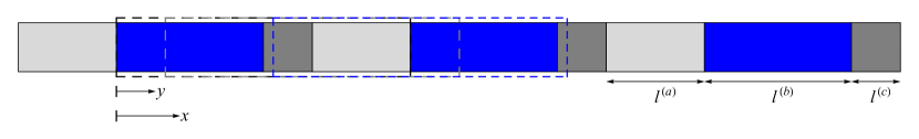
FIG. 5: Part of an infinite medium made of a periodic cell with three layers. The medium can be analyzed as random, when considering different realizations generated by periodic cells whose corner varies with $y$—a uniformly distributed variable; three of which are boxed in dashed lines.

We return to calculate $u_{\mathrm{p}}^{\pm}\left(x\right)$ by employing a standard transfer matrix approach [70, 71], as follows. The phase-wise solution of the Eq. (C.1) is

$$u(x)=\left\{\begin{array}[]{l}u^{\left(a\right)}=\alpha^{(a)}\cos k^{(a)}x+\beta^{(a)}\sin k^{(a)}x,\;\;\;-l^{(a)}<x<0,\\[3.0pt] u^{\left(b\right)}=\alpha^{(b)}\cos k^{(b)}x+\beta^{(b)}\sin k^{(b)}x,\;\;\;0<x<l^{(b)},\\[3.0pt] u^{\left(c\right)}=\alpha^{(c)}\cos k^{(c)}x+\beta^{(c)}\sin k^{(c)}x,\;\;\;l^{(b)}<x<l^{(b)}+l^{(c)},\end{array}\right.$$ (C.10)

where $\alpha^{\left(n\right)}$ and $\beta^{\left(n\right)}$ are integration constants,

$$k^{\left(n\right)}=s\sqrt{\dfrac{\rho^{\left(n\right)}}{\check{C}^{\left(n\right)}}},\quad\check{C}^{\left(n\right)}=C^{\left(n\right)}+\dfrac{\left\{B^{\left(n\right)}\right\}^{2}}{A^{\left(n\right)}},\ n=a,b,c,$$

and to abbreviate notation, we momentarily suppress the subscript $0$. The integration constants $\alpha^{\left(n\right)}$ and $\beta^{\left(n\right)}$ are determined from the continuity and Bloch-Floquet conditions on $u(x)$ and the stress $\sigma(x)$, which are compactly written using the state vectors $\mathsf{s}^{\left(n\right)}\left(x\right)$ and transfer matrices $\mathsf{T}^{\left(n\right)}$

$$\mathsf{s}^{\left(n\right)}\left(x\right)=\left(\begin{array}[]{c}u^{\left(n\right)}\\ \sigma^{\left(n\right)}\end{array}\right),\quad\mathsf{T}^{\left(n\right)}=\left(\begin{array}[]{cc}\cos k^{\left(n\right)}l^{\left(n\right)}&\dfrac{\sin k^{\left(n\right)}l^{\left(n\right)}}{\check{C}^{\left(n\right)}k^{\left(n\right)}}\\ -\check{C}^{\left(n\right)}k^{\left(n\right)}\sin k^{\left(n\right)}l^{\left(n\right)}&\cos k^{\left(n\right)}l^{\left(n\right)}\end{array}\right).$$ (C.11)

Thus, the state vectors at the ends of each layer are related via

$$\mathsf{s}^{\left(n\right)}\left(x^{\left(n\right)}+l^{\left(n\right)}\right)=\mathsf{T}^{\left(n\right)}\mathsf{s}^{\left(n\right)}\left(x^{\left(n\right)}\right),\quad x^{\left(n\right)}=-l^{\left(a\right)},0,l^{\left(b\right)}.$$ (C.12)

where continuity conditions at the interfaces are

$$\mathsf{s}^{\left(n\right)}\left(x^{\left(n\right)}+l^{\left(n\right)}\right)=\mathsf{s}^{\left(n+1\right)}\left(x^{\left(n\right)}+l^{\left(n\right)}\right),\quad x^{\left(n\right)}=0,l^{\left(b\right)},$$ (C.13)

which are combined to obtain

$$\mathsf{s}^{\left(c\right)}\left(l^{\left(c\right)}\right)=\mathsf{T}^{\Omega_{\mathrm{p}}}\mathsf{s}^{\left(a\right)}\left(-l^{\left(a\right)}\right), \mathsf{T}^{\Omega_{\mathrm{p}}}=\mathsf{T}^{(c)}\mathsf{T}^{(b)}\mathsf{T}^{(a)}.$$ (C.14)

The latter quantities are also related via the (Bloch) Floquet quasi-periodicity condition

$$\mathsf{s}^{\left(c\right)}\left(l^{\left(c\right)}\right)=e^{ik_{B}l}\mathsf{s}^{\left(a\right)}\left(-l^{\left(a\right)}\right),$$ (C.15)

Eqs. (C.14)-(C.15) deliver together the eigenvalue problem

$$\left(\mathsf{T}^{\Omega_{\mathrm{p}}}-e^{i{k}_{\mathit{B}}l}\mathsf{I}\right)\mathsf{s}=\mathsf{0}.$$ (C.16)

The standard condition for non-trivial solutions provides the dispersion relation

$$\cos k_{B}l=\frac{\mathrm{tr}\mathsf{T}^{\Omega_{\mathrm{p}}}}{2},$$ (C.17)

which, upon substitution back into the foregoing equations, provides the eigenmodes as functions of $k_{B}$, and specifically $u^{\pm}=u_{\mathrm{p}}^{\pm}\left(x\right)e^{\pm ik_{B}x}$.

In the calculations to follow is more convenient to use the Fourier expansion of of $u_{\mathrm{p}}^{+}$ and $u_{\mathrm{p}}^{-}$. Accordingly, in terms of the Fourier coefficients

$$a_{m}(\pm{k}_{\mathit{B}}) =\dfrac{1}{l}\int_{-l^{(a)}}^{l^{(b)}+l^{(c)}}u^{\pm}(x)e^{\mp i{k}_{\mathit{B}}x}e^{\frac{2i\pi mx}{l}}\mathrm{d}x,$$ (C.18)

the ensemble average of $G$

$$\left\langle G\right\rangle\left(x,x^{\prime}\right)=\frac{1}{l}\int_{\Omega_{\mathrm{p}}}G_{y}\left(x,x^{\prime}\right)\mathrm{d}y,\quad G_{y}\left(x,x^{\prime}\right)=G_{0}\left(x-y,x^{\prime}-y\right),$$ (C.19)

namely,

$$\left\langle G\right\rangle\left(x,x^{\prime}\right)=V\,e^{-i{k}_{\mathit{B}}\lvert x-x^{\prime}\lvert}\sum_{m=-\infty}^{m=\infty}a_{m}({k}_{\mathit{B}})a_{-m}(-{k}_{\mathit{B}})\,e^{\frac{2i\pi m\lvert x-x^{\prime}\lvert}{l}},$$ (C.20)

confirming it depends on $x$ and $x^{\prime}$ solely via $x-x^{\prime}$. Its Fourier transform

$$\left\langle G\right\rangle\left(\xi\right)=\int_{\Omega_{\mathrm{p}}}\left\langle G\right\rangle\left(x\right)e^{i\xi x}$$ (C.21)

reads

$$\left\langle G\right\rangle(\xi)=2V\,\sum_{m=-\infty}^{m=\infty}a_{m}({k}_{\mathit{B}})a_{-m}(-{k}_{\mathit{B}})\dfrac{i\left({k}_{\mathit{B}}-\dfrac{2\pi m}{l}\right)}{\xi^{2}-\left({k}_{\mathit{B}}-\dfrac{2\pi m}{l}\right)^{2}}.$$ (C.22)

We proceed to calculate the rest of the terms in the Fourier transform of $\tilde{\mathsf{L}}.$ To this end, we define the Fourier coefficients

$$\rho_{m}(\pm{k}_{\mathit{B}}) =\dfrac{1}{l}\int_{-l^{(a)}}^{l^{(b)}+l^{(c)}}\rho_{0}(x)e^{\mp i{k}_{\mathit{B}}x}u^{\pm}(x)e^{\frac{2i\pi mx}{l}}\mathrm{d}x,$$ (C.23)

$$\varsigma_{m}(\pm{k}_{\mathit{B}}) =\dfrac{1}{l}\int_{-l^{(a)}}^{l^{(b)}+l^{(c)}}\varsigma_{0}(x)e^{\mp i{k}_{\mathit{B}}x}u^{\pm}_{,x}(x)e^{\frac{2i\pi mx}{l}}\mathrm{d}x,\quad\varsigma=C,\check{C},\dfrac{B}{A},\dfrac{B^{2}}{A},$$ (C.24)

and obtain

$$\left\langle\varsigma(x)G{}_{,x}\right\rangle(\xi) = V\sum_{m=-\infty}^{m=\infty}\left[\dfrac{\varsigma_{m}({k}_{\mathit{B}})a_{-m}(-{k}_{\mathit{B}})}{\vartheta_{m}^{+}}+\dfrac{\varsigma_{-m}(-{k}_{\mathit{B}})a_{m}({k}_{\mathit{B}})}{\vartheta_{m}^{-}}\right],$$ (C.25)

$$\left\langle\varsigma_{\mathrm{\left(1\right)}}(x)G{}_{,x}\varsigma_{\mathrm{\mathrm{\left(2\right)}}}(x^{\prime})\right\rangle(\xi) = V\sum_{m=-\infty}^{m=\infty}\left[\dfrac{\varsigma_{\mathrm{\mathrm{\left(1\right)}}m}({k}_{\mathit{B}})\varsigma_{\mathrm{\left(2\right)}-m}(-{k}_{\mathit{B}})}{\vartheta_{m}^{+}}+\dfrac{\varsigma_{\mathrm{\mathrm{\left(1\right)}-m}}(-{k}_{\mathit{B}})\varsigma_{\mathrm{\left(2\right)}m}({k}_{\mathit{B}})}{\vartheta_{m}^{-}}\right],$$ (C.27)

$$\left\langle\varsigma(x)G{}_{,xx^{\prime}}\varsigma(x^{\prime})\right\rangle(\xi) = V\sum_{m=-\infty}^{m=\infty}\left[\dfrac{\varsigma_{m}({k}_{\mathit{B}})\varsigma_{-m}(-{k}_{\mathit{B}})}{\vartheta_{m}^{+}}+\dfrac{\varsigma_{\mathrm{-m}}(-{k}_{\mathit{B}})\varsigma_{m}({k}_{\mathit{B}})}{\vartheta_{m}^{-}}\right]+\left\langle\varsigma\right\rangle,$$ (C.28)

$$\left\langle\varsigma_{\mathrm{\left(1\right)}}(x)G{}_{,xx^{\prime}}\varsigma_{\mathrm{\left(2\right)}}(x^{\prime})\right\rangle(\xi) = V\sum_{m=-\infty}^{m=\infty}\left[\dfrac{\varsigma_{\mathrm{\left(1\right)}m}({k}_{\mathit{B}})\varsigma_{\mathrm{\left(2\right)}-m}(-{k}_{\mathit{B}})}{\vartheta_{m}^{+}}+\dfrac{\varsigma_{\mathrm{\left(1\right)-m}}(-{k}_{\mathit{B}})\varsigma_{\mathrm{\left(2\right)}m}({k}_{\mathit{B}})}{\vartheta_{m}^{-}}\right]+\left\langle\varsigma_{\mathrm{\left(1\right)}}\right\rangle,$$

$$\left\langle\rho(x)G\right\rangle(\xi) = V\sum_{m=-\infty}^{m=\infty}\left[\dfrac{\rho_{m}({k}_{\mathit{B}})a_{-m}(-{k}_{\mathit{B}})}{\vartheta_{m}^{+}}+\dfrac{\rho_{-m}(-{k}_{\mathit{B}})a_{m}({k}_{\mathit{B}})}{\vartheta_{m}^{-}}\right],$$ (C.29)

$$\left\langle\rho(x)G\rho(x^{\prime})\right\rangle(\xi) = V\sum_{m=-\infty}^{m=\infty}\left[\dfrac{\rho_{m}({k}_{\mathit{B}})\rho_{-m}(-{k}_{\mathit{B}})}{\vartheta_{m}^{+}}+\dfrac{\rho_{-m}(-{k}_{\mathit{B}})\rho_{m}({k}_{\mathit{B}})}{\vartheta_{m}^{-}}\right],$$ (C.30)

where $\varsigma_{\mathrm{\left(1\right)}}$ and $\varsigma_{\mathrm{\left(2\right)}}$ denote two different properties from the set $\left\{C,\check{C},\dfrac{B}{A},\dfrac{B^{2}}{A}\right\}$, and

$$\vartheta_{m}^{\pm}=i\left({k}_{\mathit{B}}-\dfrac{2\pi m}{l}\pm\xi\right).$$

Note that

$$\left\langle G{}_{,x^{\prime}}\rho(x^{\prime})\right\rangle(\xi) = \left\langle\rho(x)G{{}_{,x}}\right\rangle(-\xi),$$ (C.31)

$$\left\langle\varsigma_{\mathrm{\left(2\right)}}(x)G{}_{,x^{\prime}}\varsigma_{\mathrm{\mathrm{\left(1\right)}}}(x^{\prime})\right\rangle(\xi) = \left\langle\varsigma_{\mathrm{\left(1\right)}}(x)G{}_{,x}\varsigma_{\mathrm{\mathrm{\left(2\right)}}}(x^{\prime})\right\rangle(-\xi),$$ (C.32)

$$\left\langle G\rho(x^{\prime})\right\rangle(\xi) = \left\langle\rho(x)G\right\rangle(-\xi).$$ (C.33)

The process is exemplified using the calculation of $\left\langle C(x)\,G{{}_{,x}}\right\rangle(\xi)$. Firstly, note that in realization $y=0$ is

$$C_{0}(x)G_{0,x}=\left\{\begin{array}[]{l}VC_{0}(x)u^{+}_{,x}(x)u^{-}(x^{\prime}),\;\;\;x<x^{\prime},\\[10.0pt] Vu^{+}(x^{\prime})C_{0}(x)u^{-}_{,x}(x),\;\;\;x^{\prime}<x.\end{array}\right.$$ (C.36)

The translated expression is thus

$$C(x)G{{}_{,x}}=\left\{\begin{array}[]{l}Ve^{i{k}_{\mathit{B}}(x-x^{\prime})}\sum\limits_{m=-\infty}^{m=\infty}C_{m}({k}_{\mathit{B}})e^{\frac{-2i\pi m(x-y)}{l}}\sum\limits_{n=-\infty}^{n=\infty}a_{n}(-{k}_{\mathit{B}})e^{\frac{-2i\pi n(x^{\prime}-y)}{l}},\;\;\;x<x^{\prime}\\[10.0pt] Ve^{i{k}_{\mathit{B}}(x^{\prime}-x)}\sum\limits_{m=-\infty}^{m=\infty}a_{m}({k}_{\mathit{B}})e^{\frac{-2i\pi m(x^{\prime}-y)}{l}}\sum\limits_{n=-\infty}^{n=\infty}C_{n}(-{k}_{\mathit{B}})e^{\frac{-2i\pi n(x-y)}{l}}\;\;\;x^{\prime}<x.\end{array}\right.$$ (C.37)

It follows that

$$\left\langle C(x)\,G{{}_{,x}}\right\rangle\,(x-x^{\prime})=\left\{\begin{array}[]{l}Ve^{i{k}_{\mathit{B}}(x-x^{\prime})}\sum\limits_{m=-\infty}^{m=\infty}C_{m}({k}_{\mathit{B}})a_{-m}(-{k}_{\mathit{B}})e^{\frac{2i\pi m(x^{\prime}-x)}{l}},\;\;\;x<x^{\prime}\\[10.0pt] Ve^{i{k}_{\mathit{B}}(x^{\prime}-x)}\sum\limits_{m=-\infty}^{m=\infty}a_{m}({k}_{\mathit{B}})C_{-m}(-{k}_{\mathit{B}})e^{\frac{2i\pi m(x-x^{\prime})}{l}}\;\;\;x^{\prime}<x,\end{array}\right.$$ (C.40)

and its Fourier transform is

$$\left\langle C(x)G{{}_{,x}}\right\rangle(\xi)=V\sum_{m=-\infty}^{m=\infty}\left[\dfrac{C_{m}({k}_{\mathit{B}})a_{-m}(-{k}_{\mathit{B}})}{i\left({k}_{\mathit{B}}-\dfrac{2\pi m}{l}+\xi\right)}+\dfrac{a_{m}({k}_{\mathit{B}})C_{-m}(-{k}_{\mathit{B}})}{i\left({k}_{\mathit{B}}-\dfrac{2\pi m}{l}-\xi\right)}\right].$$ (C.41)

Appendix D. Explicit expressions for the effective properties

Recall that in the present problem

$$\sigma=\left(C+\dfrac{B^{2}}{A}\right)\left(u_{,x}-\eta\right),\;\;\;\phi{}_{,x}=\dfrac{B}{A}\left(u_{,x}-\eta\right),\;\;\;D=0,\;\;\;p=s\rho u,$$ (D.1)

and hence

$$\left\langle\sigma\right\rangle=\left\langle\left(C+\dfrac{B^{2}}{A}\right)\left(u_{,x}-\eta\right)\right\rangle,\;\;\;\left\langle\phi_{,x}\right\rangle=\left\langle\dfrac{B}{A}\left(u_{,x}-\eta\right)\right\rangle,\;\;\;\left\langle D\right\rangle=0,\;\;\;\left\langle p\right\rangle=\left\langle s\rho u\right\rangle.$$ (D.2)

In terms of the effective properties, we we also have that

$$\begin{aligned} \left\langle\sigma\right\rangle&=\left(\tilde{C}+\dfrac{\tilde{B}^{\mathsf{T}}\tilde{B}}{\tilde{A}}\right)\left(\left\langle u_{,x}\right\rangle-\eta\right)+\left(\tilde{S}+\tilde{B}^{\mathsf{T}}\dfrac{\tilde{W}}{\tilde{A}}\right)\left\langle su\right\rangle,\\[3.0pt] \left\langle\phi_{,x}\right\rangle&=\dfrac{\tilde{B}}{\tilde{A}}\left(\left\langle u_{,x}\right\rangle-\eta\right)+\dfrac{\tilde{W}}{\tilde{A}}\left\langle su\right\rangle,\\[3.0pt] \left\langle p\right\rangle&=\left(\tilde{S}^{\dagger}+\tilde{W}^{\dagger}\dfrac{\tilde{B}}{\tilde{A}}\right)\left(\left\langle u_{,x}\right\rangle-\eta\right)+\left(\tilde{\rho}+\dfrac{\tilde{W}\tilde{W}^{\dagger}}{\tilde{A}}\right)\left\langle su\right\rangle.\end{aligned}$$ (D.3)

By substituting

$$\begin{aligned} u\left(x,y\right)=&\left(G\left\langle G\right\rangle{}^{-1}\left\langle G_{,x^{\prime}}\check{C}\right\rangle-G{}_{,x^{\prime}}\check{C}\right)\left(\left\langle u_{,x^{\prime}}\right\rangle-\eta\right)\\ &+\left(G\left\langle G\right\rangle{}^{-1}\left\langle G\rho\right\rangle-G\rho\right)s^{2}\left\langle u\right\rangle+\left\langle u\right\rangle,\end{aligned}$$ (D.4)

into Eq. (D.2) and comparing with Eq. (D.3) we obtain

$$\tilde{C}+\dfrac{\tilde{B}^{\mathsf{T}}\tilde{B}}{\tilde{A}} = \left\langle\check{C}\right\rangle-\left\langle\check{C}(x)G{}_{,xx^{\prime}}\check{C}(x^{\prime})\right\rangle+\left\langle\check{C}(x)G{}_{,x}\right\rangle\left\langle G\right\rangle^{-1}\left\langle G{}_{,x^{\prime}}\check{C}(x^{\prime})\right\rangle,$$

$$\tilde{S} = -s\left\langle C(x)G{}_{,x}\rho(x^{\prime})\right\rangle+s\left\langle C(x)G{}_{,x}\right\rangle\left\langle G\right\rangle^{-1}\left\langle G\rho(x^{\prime})\right\rangle,$$

$$\tilde{B}^{\mathsf{T}}\dfrac{\tilde{W}}{\tilde{A}} = -s\left\langle\dfrac{B(x)^{2}}{A(x)}G{}_{,x}\rho(x^{\prime})\right\rangle+s\left\langle\dfrac{B(x)^{2}}{A(x)}G{}_{,x}\right\rangle\left\langle G\right\rangle^{-1}\left\langle G\rho(x^{\prime})\right\rangle,$$ (D.5)

from $\left\langle\sigma\right\rangle$; from $\left\langle\phi_{,x}\right\rangle$ we find

$$\dfrac{\tilde{B}}{\tilde{A}} = \left\langle\dfrac{B}{A}\right\rangle-\left\langle\dfrac{B(x)}{A(x)}G{}_{,xx^{\prime}}\check{C}(x^{\prime})\right\rangle+\left\langle\dfrac{B(x)}{A(x)}G{}_{,x}\right\rangle\left\langle G\right\rangle^{-1}\left\langle G{}_{,x^{\prime}}\check{C}(x^{\prime})\right\rangle,$$

$$\dfrac{\tilde{W}}{\tilde{A}} = -s\left\langle\dfrac{B(x)}{A(x)}G{}_{,x}\rho(x^{\prime})\right\rangle+s\left\langle\dfrac{B(x)}{A(x)}G{}_{,x}\right\rangle\left\langle G\right\rangle^{-1}\left\langle G\rho(x^{\prime})\right\rangle,$$ (D.6)

and finally from $\left\langle p\right\rangle$

$$\tilde{S}^{\dagger} = -s\left\langle\rho(x)G{}_{,x^{\prime}}C(x^{\prime})\right\rangle+s\left\langle\rho(x)G\right\rangle\left\langle G\right\rangle^{-1}\left\langle G{}_{,x^{\prime}}C(x^{\prime})\right\rangle,$$

$$\tilde{W}^{\dagger}\dfrac{\tilde{B}}{\tilde{A}} = -s\left\langle\rho(x)G{}_{,x^{\prime}}\dfrac{B(x^{\prime})^{2}}{A(x^{\prime})}\right\rangle+s\left\langle\rho(x)G\right\rangle\left\langle G\right\rangle^{-1}\left\langle G{}_{,x^{\prime}}\dfrac{B(x^{\prime})^{2}}{A(x^{\prime})}\right\rangle,$$

$$\tilde{\rho}+\dfrac{\tilde{W}\tilde{W}^{\dagger}}{\tilde{A}} = \left\langle\rho\right\rangle-s^{2}\left\langle\rho(x)G\rho(x^{\prime})\right\rangle+s^{2}\left\langle\rho(x)G\right\rangle\left\langle G\right\rangle^{-1}\left\langle G\rho(x^{\prime})\right\rangle.$$ (D.7)

As we pointed out in the body of the paper

$$\tilde{S}\left(\xi\right) =\tilde{S}^{\dagger}\left(-\xi\right)=-\mathrm{conj}\,\tilde{S}^{\dagger}\left(\xi\right).$$ (D.8)

Also note that $\dfrac{\tilde{B}^{\mathsf{T}}\tilde{W}}{\tilde{A}}\left(\xi\right)=\dfrac{\tilde{B}\tilde{W}^{\dagger}}{\tilde{A}}\left(-\xi\right)$. As mentioned, the drawback for using a single Green function in the absence of charge is one degree of freedom in calculating $\tilde{\mathsf{L}}$, which we eliminate by enforcing $\tilde{B}^{\mathsf{T}}=\tilde{B}$. The latter condition, together with Eqs. (D.5)-(D.7) deliver the effective properties $\tilde{C},\tilde{A},\tilde{\rho},\tilde{B}$ and $\tilde{W},\tilde{W}^{\dagger}$. These satisfy

$$\tilde{c}\left(\xi\right)= \mathrm{conj}\,\tilde{c}\left(-\xi\right),\quad\tilde{c}=\tilde{C},\tilde{A},\tilde{\rho},\tilde{B},$$ (D.9)

$$\tilde{W}\left(\xi\right) =\tilde{W}^{\dagger}\left(-\xi\right)=-\mathrm{conj}\,\tilde{W}^{\dagger}\left(\xi\right),$$ (D.10)

where relation between $\tilde{W}$ and $\tilde{W}^{\dagger}$ is similar to the relation between $\tilde{S}$ and $\tilde{S}^{\dagger}$.

References

[1]
C. Truesdell and R. Toupin.
The Classical Field Theories, pages 226–858.
Springer Berlin Heidelberg, Berlin, Heidelberg, 1960.
[2]
Martin Wegener.
Metamaterials beyond optics.
Science, 342(6161):939–940, 2013.
[3]
Bastiaan Florijn, Corentin Coulais, and Martin van Hecke.
Programmable mechanical metamaterials.
Phys. Rev. Lett., 113:175503, Oct 2014.
[4]
Lucas R. Meza, Alex J. Zelhofer, Nigel Clarke, Arturo J. Mateos, Dennis M.
Kochmann, and Julia R. Greer.
Resilient 3d hierarchical architected metamaterials.
Proceedings of the National Academy of Sciences, 2015.
[5]
Muamer Kadic, Graeme W. Milton, Martin van Hecke, and Martin Wegener.
3d metamaterials.
Nature Reviews Physics, 1(3):198–210, 2019.
[6]
Yiqun Ding, Zhengyou Liu, Chunyin Qiu, and Jing Shi.
Metamaterial with Simultaneously Negative Bulk Modulus and Mass
Density.
Phys. Rev. Lett., 99(9):93904, 2007.
[7]
Huanyang Chen, C. T. Chan, and Ping Sheng.
Transformation optics and metamaterials.
Nature Materials, 9:387 EP –, 04 2010.
[8]
Biswajit Banerjee.
An introduction to metamaterials and waves in composites.
CRC Press, 2011.
[9]
Richard V Craster and Sébastien Guenneau.
Acoustic metamaterials: Negative refraction, imaging, lensing
and cloaking, volume 166.
Springer Science & Business Media, 2012.
[10]
William J. Parnell and Tom Shearer.
Antiplane elastic wave cloaking using metamaterials, homogenization
and hyperelasticity.
Wave Motion, 50(7):1140 – 1152, 2013.
Advanced Modelling of Wave Propagation in Solids.
[11]
Pai Wang, Filippo Casadei, Sicong Shan, James C. Weaver, and Katia Bertoldi.
Harnessing buckling to design tunable locally resonant acoustic
metamaterials.
Physical Review Letters, 113:014301, 2014.
[12]
Paolo Celli and Stefano Gonella.
Manipulating waves with LEGO®bricks: A versatile
experimental platform for metamaterial architectures.
Appl. Phys. Lett., 107(8), 2015.
[13]
Miguel Molerón and Chiara Daraio.
Acoustic metamaterial for subwavelength edge detection.
Nature Communications, 6:8037 EP –, 08 2015.
[14]
Steven A Cummer, Johan Christensen, and Andrea Alù.
Controlling sound with acoustic metamaterials, 2016.
[15]
A. S. Phani and M. I. Hussein, editors.
Dynamics of lattice materials.
Wiley, New York, 2017.
[16]
Bolei Deng, Vincent Tournat, Pai Wang, and Katia Bertoldi.
Anomalous collisions of elastic vector solitons in mechanical
metamaterials.
Physical Review Letters, 122:044101, 2019.
[17]
J R Willis.
Continuum Micromechanics.
chapter Dynamics o, pages 265–290. Springer-Verlag New York, Inc.,
New York, NY, USA, 1997.
[18]
Hussein Nassar, Qi-Chang He, and Nicolas Auffray.
Willis elastodynamic homogenization theory revisited for periodic
media.
Journal of the Mechanics and Physics of Solids, 2015.
[19]
Z H Xiang and R W Yao.
Realizing the Willis equations with pre-stresses.
Journal of the Mechanics and Physics of Solids, 87:1–6, 2016.
[20]
H Nassar, Q.-C. He, and N Auffray.
On asymptotic elastodynamic homogenization approaches for periodic
media.
J. Mech. Phys. Solids, 88:274–290, 2016.
[21]
Michael B Muhlestein, Caleb F Sieck, Andrea Alù, and Michael R Haberman.
Reciprocity, passivity and causality in Willis materials.
Proc. R. Soc. London A Math. Phys. Eng. Sci., 472(2194), 2016.
[22]
H Nassar, X C Xu, A N Norris, and G L Huang.
Modulated phononic crystals: Non-reciprocal wave propagation and
Willis materials.
Journal of the Mechanics and Physics of Solids, 101:10–29,
2017.
[23]
Caleb F Sieck, Andrea Alù, and Michael R Haberman.
Origins of Willis coupling and acoustic bianisotropy in acoustic
metamaterials through source-driven homogenization.
Phys. Rev. B, 96(10):104303, 2017.
[24]
Xiaoshi Su and Andrew N. Norris.
Retrieval method for the bianisotropic polarizability tensor of
willis acoustic scatterers.
Phys. Rev. B, 98:174305, Nov 2018.
[25]
Li Quan, Younes Ra’di, Dimitrios L Sounas, and Andrea Alù.
Maximum Willis Coupling in Acoustic Scatterers.
Phys. Rev. Lett., 120(25):254301, 2018.
[26]
Shixu Meng and Bojan B Guzina.
On the dynamic homogenization of periodic media: Willis’ approach
versus two-scale paradigm.
Proc. R. Soc. London A Math. Phys. Eng. Sci., 474(2213), 2018.
[27]
Sukmo Koo, Choonlae Cho, Jun-ho Jeong, and Namkyoo Park.
Acoustic omni meta-atom for decoupled access to all octants of a wave
parameter space.
Nature Communications, 7:13012 EP –, 09 2016.
[28]
Michael B. Muhlestein, Caleb F. Sieck, Preston S. Wilson, and Michael R.
Haberman.
Experimental evidence of willis coupling in a one-dimensional
effective material element.
Nature Communications, 8:15625 EP –, 06 2017.
[29]
Junfei Li, Chen Shen, Ana D’iaz-Rubio, Sergei A Tretyakov, and Steven A
Cummer.
Systematic design and experimental demonstration of bianisotropic
metasurfaces for scattering-free manipulation of acoustic wavefronts.
Nat. Commun., 9(1):1342, 2018.
[30]
Bogdan-Ioan Popa, Yuxin Zhai, and Hyung-Suk Kwon.
Broadband sound barriers with bianisotropic metasurfaces.
Nature Communications, 9(1):5299, 2018.
[31]
R W Yao, H X Gao, Y X Sun, X D Yuan, and Z H Xiang.
An experimental verification of the one-dimensional static
Willis-form equations.
Int. J. Solids Struct., 134:283–292, 2018.
[32]
Aurélien Merkel, Vicent Romero-García, Jean-Philippe Groby, Jensen Li,
and Johan Christensen.
Unidirectional zero sonic reflection in passive
-symmetric willis media.
Phys. Rev. B, 98:201102, Nov 2018.
[33]
Anton Melnikov, Yan Kei Chiang, Li Quan, Sebastian Oberst, Andrea Alù,
Steffen Marburg, and David Powell.
Acoustic meta-atom with experimentally verified maximum willis
coupling.
Nature Communications, 10(1):3148, 2019.
[34]
Yongquan Liu, Zixian Liang, Jian Zhu, Lingbo Xia, Olivier Mondain-Monval,
Thomas Brunet, Andrea Alù, and Jensen Li.
Willis metamaterial on a structured beam.
Phys. Rev. X, 9:011040, Feb 2019.
[35]
Yuxin Zhai, Hyung-Suk Kwon, and Bogdan-Ioan Popa.
Active Willis metamaterials for ultra-compact non-reciprocal linear
acoustic devices.
arXiv e-prints, page arXiv:1901.02979, Jan 2019.
[36]
Warren P Mason.
Piezoelectric crystals and their application to ultrasonics.Van Nostrand, New York, 1950.
[37]
Matthew Zelisko, Yuranan Hanlumyuang, Shubin Yang, Yuanming Liu, Chihou Lei,
Jiangyu Li, Pulickel M. Ajayan, and Pradeep Sharma.
Anomalous piezoelectricity in two-dimensional graphene nitride
nanosheets.
Nature Communications, 5:4284 EP –, 06 2014.
[38]
Mikhail Lapine, Ilya V. Shadrivov, David A. Powell, and Yuri S. Kivshar.
Magnetoelastic metamaterials.
Nature Materials, 11:30 EP –, 11 2011.
[39]
Jinwoong Cha, Kun Woo Kim, and Chiara Daraio.
Experimental realization of on-chip topological nanoelectromechanical
metamaterials.
Nature, 564(7735):229–233, 2018.
[40]
Julie A. Jackson, Mark C. Messner, Nikola A. Dudukovic, William L. Smith, Logan
Bekker, Bryan Moran, Alexandra M. Golobic, Andrew J. Pascall, Eric B. Duoss,
Kenneth J. Loh, and Christopher M. Spadaccini.
Field responsive mechanical metamaterials.
Science Advances, 4(12), 2018.
[41]
J. Shi and A.H. Akbarzadeh.
Architected cellular piezoelectric metamaterials:
Thermo-electro-mechanical properties.
Acta Materialia, 163:91 – 121, 2019.
[42]
René Pernas-Salomón and Gal Shmuel.
Tunable asymmetric reflaction in metamaterials with electro-momentum
coupling.
In preparation, 2019.
[43]
David R. Smith and John B. Pendry.
Homogenization of metamaterials by field averaging (invited paper).
J. Opt. Soc. Am. B, 23(3):391–403, Mar 2006.
[44]
Chris Fietz and Gennady Shvets.
Current-driven metamaterial homogenization.
Physica B: Condensed Matter, 405(14):2930 – 2934, 2010.
Proceedings of the Eighth International Conference on Electrical
Transport and Optical Properties of Inhomogeneous Media.
[45]
Andrea Alù.
First-principles homogenization theory for periodic metamaterials.
Phys. Rev. B, 84:075153, Aug 2011.
[46]
A L Shuvalov, A A Kutsenko, A N Norris, and O Poncelet.
Effective Willis constitutive equations for periodically stratified
anisotropic elastic media.
Proc. R. Soc. London A Math. Phys. Eng. Sci.,
467(2130):1749–1769, 2011.
[47]
Sia Nemat-Nasser, John R Willis, Ankit Srivastava, and Alireza V Amirkhizi.
Homogenization of periodic elastic composites and locally resonant
sonic materials.
Physical Review B, 83(10):104103, 2011.
[48]
Daniel Torrent and José Sánchez-Dehesa.
Multiple scattering formulation of two-dimensional acoustic and
electromagnetic metamaterials.
New Journal of Physics, 13(9):093018, sep 2011.
[49]
T Antonakakis, R V Craster, and S Guenneau.
Asymptotics for metamaterials and photonic crystals.
Proc. R. Soc. London A Math. Phys. Eng. Sci., 469(2152), 2013.
[50]
Ankit Srivastava.
Elastic metamaterials and dynamic homogenization: a review.
International Journal of Smart and Nano Materials, 6(1):41–60,
2015.
[51]
Michael B Muhlestein and Michael R Haberman.
A micromechanical approach for homogenization of elastic
metamaterials with dynamic microstructure.
Proc. R. Soc. London A Math. Phys. Eng. Sci., 472(2192), 2016.
[52]
Marie-Fraise Ponge, Olivier Poncelet, and Daniel Torrent.
Dynamic homogenization theory for nonlocal acoustic metamaterials.
Extrem. Mech. Lett., 12:71–76, 2017.
[53]
J R Willis.
Variational principles for dynamic problems for inhomogeneous
elastic media.
Wave Motion, 3(1):1–11, 1981.
[54]
John R Willis.
Variational and related methods for the overall properties of
composites.
Advances in applied mechanics, 21:1–78, 1981.
[55]
J R Willis.
The nonlocal influence of density variations in a composite.
Int. J. Solids Struct., 21(7):805–817, 1985.
[56]
J R Willis.
Exact effective relations for dynamics of a laminated body.
Mech. Mater., 41(4):385–393, 2009.
[57]
J R Willis.
Effective constitutive relations for waves in composites and
metamaterials.
Proc. R. Soc. London A Math. Phys. Eng. Sci.,
467(2131):1865–1879, 2011.
[58]
J.R. Willis.
A comparison of two formulations for effective relations for waves in
a composite.
Mechanics of Materials, 47:51 – 60, 2012.
[59]
John R. Willis.
The construction of effective relations for waves in a composite.
Comptes Rendus Mécanique, 340(4):181 – 192, 2012.
Recent Advances in Micromechanics of Materials.
[60]
Andrea Alù.
Restoring the physical meaning of metamaterial constitutive
parameters.
Phys. Rev. B, 83:081102, Feb 2011.
[61]
B.A. Auld.
Acoustic fields and waves in solids.
A Wiley-Interscience publication. Wiley, 1973.
[62]
René Pernas-Salomón and Gal Shmuel.
Dynamic homogenization of composite and locally resonant flexural
systems.
J. Mech. Phys. Solids, 119:43–59, 2018.
[63]
A N Norris, A L Shuvalov, and A A Kutsenko.
Analytical formulation of three-dimensional dynamic homogenization
for periodic elastic systems.
Proc. R. Soc. London A Math. Phys. Eng. Sci., 2012.
[64]
Ankit Srivastava and Sia Nemat-Nasser.
Overall dynamic properties of three-dimensional periodic elastic
composites.
Proceedings of the Royal Society of London A: Mathematical,
Physical and Engineering Sciences, 468(2137):269–287, 2012.
[65]
A Srivastava and S Nemat-Nasser.
On the limit and applicability of dynamic homogenization.
Wave Motion, 51(7):1045–1054, 2014.
[66]
Graeme W Milton.
The theory of composites, volume 6.
Cambridge university press, 2002.
[67]
R.B. Hetnarski and M.R. Eslami.
Thermal Stresses – Advanced Theory and Applications.
Solid Mechanics and Its Applications. Springer Netherlands, 2008.
[68]
R W Ogden.
Non-Linear Elastic Deformations.
Dover Publications, New York, 1997.
[69]
M. S. P. Eastham.
The spectral theory of periodic differential equations.
1973.
[70]
J W Dunkin.
Computation of modal solutions in layered, elastic media at high
frequencies.
Bull. Seismol. Soc. Am., 55(2):335, 1965.
[71]
G Shmuel and R Pernas-Salomón.
Manipulating motions of elastomer films by
electrostatically-controlled aperiodicity.
Smart Mater. Struct., 25(12):125012, 2016.