The methods of thermal field theory for degenerate quantum plasmas in astrophysical compact objects

Abstract

In the study of degenerate plasmas contained within compact astrophysical objects, both special relativity and general relativity play important roles. After reviewing the existing treatment in the literature, here we employ the methods of relativistic thermal quantum field theory to compute the equation of states of degenerate matter for compact astrophysical objects such as the white dwarfs and the neutron stars. In particular, we compute the equation of states that include leading order corrections due to the finite temperature, the fine-structure constant as well as the effect of gravitational time dilation. We show that the fine-structure constant correction remains well-defined even in the non-relativistic regime in contrast to the existing treatment in the literature.

I Introduction

It is not often that one sees a path-breaking discovery like the observation of gravitational waves that pushes the boundary of the fundamental physics into a new frontier. The existence of such waves arising from the fluctuations of the very fabric of the spacetime, was predicted from Einstein’s general relativity nearly a century ago. However, the experimental detection of these waves has required an unprecedented level of progress in the instrumentation techniques and data analysis methods. The very first observation that was made by the gravitational wave detectors, is thought to have originated from the merger event of two black holes ¹. Subsequently, these gravitational wave detectors have detected signals from the merger events of binary neutron stars. Remarkably, this event was also accompanied with the electromagnetic signals which were captured by multiple telescopes over a wide electromagnetic spectrum ². This unprecedented observation of a given event through both electromagnetic waves and gravitational waves has led to an era of the so-called multi-messenger astronomy. Apart from the already operational ground-based gravitational wave detectors, the future space-based gravitational wave detectors, such as LISA ³, are also under active consideration. These detectors will potentially detect gravitational wave signals from the merger events involving the white dwarf stars.

The common aspect of these gravitational waves detectors is that they are primarily designed to observe gravitational waves which essentially originate from the coalescence events involving various massive yet compact astrophysical objects. These compact astrophysical objects are primarily the black holes, the neutron stars and the white dwarfs. Among these astrophysical objects, the most compact objects are the black holes whose interior spacetime are screened by an event horizon from where even the light cannot escape. This property of the event horizon essentially limits the possibility of understanding the interior black hole spacetime even in principle. The next most compact astrophysical objects are the neutron stars. For example, the neutron star in the well-known Hulse -Taylor binary pulsar system has a mass of around $1.4M_{\odot}$ whereas it has a radius of only about ten kilometer or so ^{4, 5}. Such a compact object would require its interior energy density to be order of the nuclear density and the interior matter to be in some form of a nuclear matter plasma. The least compact objects, among the astrophysical objects under consideration, are the white dwarf stars or simply the white dwarfs. For example, the famous white dwarf Sirius B whose mass is almost equal to the mass of Sun but has a radius which is even less than the radius of the planet Earth. A simple calculation would show that even for the white dwarfs interior matter density is so high that on the average an electron has lesser space inside a white dwarf than the space which is required for the electron to be in an atomic orbital. Clearly, inside the white dwarfs the matter can only be in the form of a plasma as the atoms themselves are smashed by the enormous gravitational pull. However, the electrons in the case of white dwarfs or the neutrons in the case of neutron stars are fermions and due to Pauli’s exclusion principle, these fermions resist being compressed to an extreme density. The resultant pressure of quantum mechanical origin that counters the gravitational pull to make these stars stable, is usually known as the degeneracy pressure.

Clearly, in the view of gravitational wave observations with an unprecedented precision, it has become a necessity to understand the physics of these compact astrophysical objects in a much more detailed manner. This in turn demands one to study the properties of the degenerate quantum plasmas that are present within these objects, using the best possible theoretical framework that are known today. Here we describe the degenerate quantum plasmas inside the self-gravitating stars by using the methods of quantum field theory in curved spacetime. In particular, we consider Einstein’s equation of general relativity which is of the form $G_{\mu\nu}=8\pi G~{}\langle\hat{T}_{\mu\nu}\rangle$ where $\langle.\rangle$ denotes the thermal expectation value. In this formulation, the matter degrees of freedom, represented by the stress-energy tensor ${T}_{\mu\nu}$, are described by the quantum theory. On the other hand, the spacetime curvature, represented by the Einstein tensor $G_{\mu\nu}$, is described by the classical theory. We may emphasize here that we do not use any quantum theory of gravity. Firstly, the quest for a quantum theory of gravity is still an area of active research. Secondly, for compact stars such as the white dwarfs or the neutron stars, the quantum gravity corrections are expected to be rather negligible, as the energy scales associated with these stars are extremely small compared to the Planck scale, the presumed scale of quantum gravity.

In this review, we begin by considering a system of degenerate quantum plasmas in the background of Minkowski spacetime. Such descriptions are directly relevant for describing the equation of state (EOS) corresponding to the plasma of degenerate electrons which are present within the white dwarfs. For these stars, the effects of general relativity are relatively smaller. In order to describe degenerate plasma inside the white dwarfs one also needs to consider electromagnetic interaction between the electrons themselves and also between the electrons and the positively charged nuclei. Subsequently, we consider the effects of general relativity on the equation of states of these degenerate plasmas. In particular, we study the equation of state of the degenerate plasmas which are located within a spherically symmetric curved spacetime. We then consider the effects of these corrections on the mass-radius relations of the white dwarfs. On the other hand, due to the limitations in understanding of the dense nuclear matter physics, the understanding of the degenerate plasmas present within the neutron stars are still an active area of ongoing research. Nevertheless, the simplest form of degenerate plasma inside the neutron star can be viewed as an ensemble of degenerate neutrons. These neutrons being neutral particles they do not interact electromagnetically. The corresponding equation of state can be obtained from the equation of state of degenerate electrons by suitably mapping the parameters and turning off the electromagnetic interactions. Thereafter, we briefly discuss about a widely used realistic model, the so-called the $\sigma-\omega$ model, to describe the degenerate nuclear matter present within the neutron stars.

II Degenerate plasma in flat spacetime

In the study of degenerate matter within the white dwarfs, as pioneered by Chandrasekhar ^{6, 7}, the degenerate electrons are treated as free particles which follow the Fermi-Dirac statistics. The effect of electromagnetic interaction on the degenerate matter in the white dwarfs, by the means of ‘classical’ Coulomb energy, was first considered by Frenkel ⁸, and was followed up by Kothari ⁹, Auluck and Mathur ¹⁰. However, a more accurate study on various corrections to the equation of state due to the so-called Coulomb effects was done by Salpeter ¹¹. The implications of these corrections on the mass-radius relation of the white dwarfs were carried out by Hamada, Salpeter ¹² and Nauenberg ¹³.

One may classify the total Coulomb effects that are considered by Salpeter into following broad components (see also ^{14, 15}). (a) The ‘classical’ Coulomb energy includes the electrostatic energy of uniformly distributed degenerate electrons within the Wigner-Seitz cells, each surrounding a positively charged nucleus within a rigid lattice. It includes the electron-nuclei interaction and the self-interaction of electrons. (b) The Thomas-Fermi correction arises due to the radial variation of electron density within a Wigner-Seitz cell. (c) The ‘exchange energy’ and the ‘correlation energy’ arise due to the transverse interactions between two electrons, essentially due to the Lorentz force between them apart from its electrostatic component which is already included in (a). We may mention here that the Thomas-Fermi model is a non-relativistic model and relativistic corrections to it have been considered for the white dwarfs in Ref. ^{16, 17, 18}.

The special relativity plays a key role in the white dwarf physics. In particular, the existence of the Chandrasekhar upper mass limit for the white dwarfs arises essentially due to the special relativity which demands that the physical results should be invariant under the Lorentz transformations. Unfortunately, the methods employed in computing the Coulomb effects to the equation of state of the white dwarfs use electrostatic considerations which are non-relativistic ab initio. Therefore, from the fundamental point of view these computations should be viewed as an approximation of the corrections that one would expect from a Lorentz invariant computation. Further, these computations are usually performed at the zero temperature ¹¹ (however see ^{19, 20, 21}). the future detection of low-frequency gravitational waves from the extreme mass-ratio merger of a black hole and a white dwarf could determine the equation of state of the degenerate matter within the white dwarfs with very high accuracy ²². Such an accuracy could probe the extent of Coulomb effects and hence provides additional motivation to revisit the corrections to the equation of state of the white dwarfs.

In order to compute the equation of state for the white dwarfs, a natural arena which respects Lorentz symmetry, is provided by the relativistic thermal quantum field theory, also referred to as the finite temperature relativistic quantum field theory. Following the pioneering work of Matsubara ²³, the techniques of finite-temperature quantum field theory was employed in the context of quantum electrodynamics (QED) by Akhiezer and Peletminskii ²⁴, and later by Freedman and McLerran ²⁵, to compute the ground state energy of the relativistic electron gas that includes corrections due to the fine-structure constant. However, these treatments are insufficient to describe the degenerate matter in the white dwarfs as they do not describe the dominant interaction, as seen in non-relativistic computations, between the degenerate electrons and positively charged heavier nuclei. Therefore, in this review article, to describe the degenerate matter within the white dwarfs using the framework of finite temperature quantum field theory, we consider an additional interaction between the electrons and positively charged nuclei, described by a Lorentz invariant action, together with the quantum electrodynamics.

II.1 The scale of degeneracy

In order to understand the associated scales of the degenerate matter, let us consider the white dwarf star Sirius B which has observational mass $M=1.0~{}M_{\odot}$, radius $R=0.008~{}R_{\odot}$ and the effective temperature $T=25922~{}\mathrm{K}$ ²⁶. Therefore, its mass density is $\rho\approx 2.8\times 10^{6}~{}g/cm^{3}$. In natural units that we follow here (i.e. speed of light $c$ and Planck constant $\hbar$ are set to unity), a fully degenerate core implies that the electron density is $n_{e}\approx 6.4\times 10^{15}~{}\mathrm{(eV)^{3}}$. The corresponding Fermi momentum is $k_{F}\simeq(3\pi^{2}n_{e})^{1/3}\approx 5.7\times 10^{5}~{}\mathrm{eV}$. The associated temperature scale of the white dwarfs $\beta^{-1}\equiv k_{B}T=2.2~{}\mathrm{eV}$ then leads to a dimensionless parameter

$$\beta k_{F}\approx 2.6\times 10^{5}~{},$$ (1)

which plays an important role in characterizing the degenerate matter within the white dwarf stars.

II.2 Dirac spinor field

In order to compute the equation of state of the degenerate matter, we consider the spacetime within a white dwarf star to be described by the Minkowski metric $\eta_{\mu\nu}=diag(-1,1,1,1)$ i.e. for time being we ignore the corrections from the general relativity (as also done by Salpeter ¹¹). Nevertheless, we shall be considering these corrections arising from the general relativity in a later section. The degenerate electrons are fermionic degrees of freedom and are represented by the Dirac spinor field $\psi$ along with the action

$$S_{\psi}=\int d^{4}x\mathcal{L}_{\psi}=-\int d^{4}x\sqrt{-\eta}~{}\overline{\psi}[i\gamma^{\mu}\partial_{\mu}+m]\psi~{},$$ (2)

where $\eta=det(\eta_{\mu\nu})=-1$ and $m$ is the mass of the field. The Dirac matrices $\gamma^{\mu}$ satisfy the anti-commutation relation

$$\{\gamma^{\mu},\gamma^{\nu}\}=-2\eta^{\mu\nu}\mathbb{I}~{}.$$ (3)

The minus sign in front of $\eta^{\mu\nu}$ in the Eq. (3) is chosen such that for given metric signature, the Dirac matrices satisfy the usual relations $(\gamma^{0})^{2}=\mathbb{I}$ and $(\gamma^{k})^{2}=-\mathbb{I}$ for $k=1,2,3$. In Dirac representation, these matrices can be expressed as

$$\gamma^{0}=\begin{pmatrix}\mathbb{I}&0\\ 0&-\mathbb{I}\end{pmatrix}~{}~{},~{}~{}\gamma^{k}=\begin{pmatrix}0&\sigma^{k}\\ -\sigma^{k}&0\end{pmatrix}~{},$$ (4)

where Pauli matrices $\sigma^{k}$ are given by

$$\sigma^{1}=\begin{pmatrix}0&1\\ 1&0\end{pmatrix}~{}~{},~{}~{}\sigma^{2}=\begin{pmatrix}0&-i\\ i&0\end{pmatrix}~{}~{},~{}~{}\sigma^{3}=\begin{pmatrix}1&0\\ 0&-1\end{pmatrix}~{}.$$ (5)

II.3 Gauge field

The electromagnetic interaction between the fermions are mediated by the gauge fields $A_{\mu}$ whose free dynamics is governed by the Maxwell action

$$S_{A}=\int d^{4}x\mathcal{L}_{A}=\int d^{4}x~{}\left[-\frac{1}{4}F_{\mu\nu}F^{\mu\nu}\right]~{},$$ (6)

where the field strength $F_{\mu\nu}=\partial_{\mu}A_{\nu}-\partial_{\nu}A_{\mu}$.

II.4 Field interactions

The degenerate electrons within a white dwarf experience two kinds of interactions, namely the self-interaction between the electrons and the interaction between electrons and the positively charge nuclei. The self-interaction between the electrons are mediated by gauge fields $A_{\mu}$ and governed by the interaction term of the quantum electrodynamics

$$S_{I}^{-}=\int d^{4}x\mathcal{L}_{I}^{-}=\int d^{4}x~{}\bar{\psi}[e~{}\gamma^{\mu}A_{\mu}]\psi~{},$$ (7)

where the parameter $e$ is the dimensionless coupling constant.

We may recall that the conserved 4-current corresponding to the action (2) is given by $j^{\mu}=\bar{\psi}\gamma^{\mu}\psi$ which represents the contribution of the electrons. Similarly, we may consider a background 4-current, say $J^{\mu}$, to represent the contributions from the nuclei. Therefore, we may model the attractive interaction between the electrons and the positively charged nuclei by a Lorentz invariant action containing the current-current interaction

$$S_{I}^{+}=\int d^{4}x\mathcal{L}_{I}^{+}=\int d^{4}x~{}[-Ze^{2}d^{2}~{}J_{\mu}\bar{\psi}\gamma^{\mu}\psi]~{},$$ (8)

where the coupling constant contains the term $-Ze^{2}$ which signifies the strength of the attractive interactions between an electron and a positively charged nucleus with atomic number $Z$. The parameter $d$ is introduced in order to make the action (8) dimensionless. It has the dimension of length and and it represents an effective length scale associated with the current-current interaction.

Therefore, the total action that describes the dynamics of the degenerate electrons within a white dwarf can be written as

$$S=S_{\psi}+S_{A}+S_{I}=S_{QED}+S_{I}^{+}~{},$$ (9)

where $S_{I}=S_{I}^{-}+S_{I}^{+}$. The inclusion of the additional interaction term (8) preserves the symmetry of the action of quantum electrodynamics $S_{QED}$. In other words, apart from being Lorentz invariant, the total action (9) is also invariant under local U(1) gauge transformations $A_{\mu}\rightarrow A_{\mu}-\frac{1}{e}\partial_{\mu}\alpha(x)$ and $\psi(x)\rightarrow e^{i\alpha(x)}\psi(x)$ with $\alpha(x)$ being an arbitrary function. Given the coupling constant $e$ is small, we can study the interacting theory by using perturbative techniques.

II.5 Partition function

In a spherically symmetric star, the pressure and the energy density both vary along the radial direction. On the other hand, in order to apply the techniques of finite temperature quantum field theory we need to consider a spatial region which is in thermal equilibrium at a given temperature $T$. Within such a region thermodynamical quantities such as the pressure and the density are uniform. Therefore, in order to deal with both these aspects we consider here a finite spatial box at a given radial coordinate. The box is assumed to be sufficiently small so that the pressure and the density remain uniform within the box yet it is sufficiently large to contain enough degrees of freedom to achieve required thermodynamical equilibrium. The corresponding partition function, describing the degrees of freedom within the box, can be expressed as

$$\mathcal{Z}=Tr\left[e^{-\beta(\hat{H}-\mu\hat{Q})}\right]~{},$$ (10)

where $\beta=1/k_{B}T$ with $k_{B}$ being the Boltzmann constant, $\mu$ refers to chemical potential and $Q$ is the conserved charge of the system. The Hamiltonian operator $\hat{H}$ represents the matter fields described by the action (9). The trace operation is carried out over the degrees of freedom contained within the specified spatial region.

II.5.1 Partition function for free fermions

The action (2) of free spinor field is invariant under a global U(1) gauge transformations $\psi(x)\rightarrow e^{i\alpha}\psi(x)$ where $\alpha$ is an arbitrary constant. Consequently, there exists an associated conserved current $j^{\mu}=\bar{\psi}\gamma^{\mu}\psi$ such that $\partial_{\mu}j^{\mu}=0$. Then the corresponding conserved charge can be expressed as $Q=\int d^{3}\mathbf{x}~{}j^{0}(x)=\int d^{3}\mathbf{x}~{}\bar{\psi}\gamma^{0}\psi$. Additionally, the conjugate field momentum corresponding to the spinor field $\psi(x)$ can be expressed as $\pi(x)=\frac{\partial\mathcal{L}_{\psi}}{\partial(\partial_{0}\psi)}=-i\bar{\psi}\gamma^{0}=-i\psi^{\dagger}$. Therefore, the partition function which contains contributions only from free spinor field can be expressed using path integral method ²⁷ as

$$\mathcal{Z}_{\psi}=\int\mathcal{D}\bar{\psi}\mathcal{D}\psi~{}e^{-S_{\psi}^{\beta}}~{},$$ (11)

where

$$S_{\psi}^{\beta}=\int_{0}^{\beta}d\tau\int d^{3}\mathbf{x}~{}\left[\mathcal{L}_{\psi}^{E}-\mu\bar{\psi}(\tau,\mathbf{x})\gamma^{0}\psi(\tau,\mathbf{x})\right]~{}.$$ (12)

The Euclidean Lagrangian density $\mathcal{L}_{\psi}^{E}$ is obtained by substituting $t\to-i\tau$ in Lagrangian density $\mathcal{L}_{\psi}$ and can be expressed as

$$\mathcal{L}_{\psi}^{E}=\bar{\psi}(\tau,\mathbf{x})[-\gamma^{0}\partial_{\tau}+i\gamma^{k}\partial_{k}+m]\psi(\tau,\mathbf{x})~{},$$ (13)

where $k=1,2,3$. In the functional integral (11), the spinor field is subject to anti-periodic boundary conditions given by

$$\psi(\tau,\mathbf{x})=-\psi(\tau+\beta,\mathbf{x})~{}~{};~{}~{}\bar{\psi}(\tau,\mathbf{x})=-\bar{\psi}(\tau+\beta,\mathbf{x})~{}.$$ (14)

It is convenient to express the partition function using the Matsubara frequencies and wave-vector by transforming the field in Fourier domain as

$$\psi(\tau,\mathbf{x})=\frac{1}{\sqrt{V}}\sum_{n,\mathrm{k}}~{}e^{-i(\omega_{n}\tau+\mathrm{k}\cdot\mathbf{x})}\tilde{\psi}(n,\mathrm{k})~{},$$ (15)

where $V$ denotes the spatial volume of the box. The Eq. (14) then implies that the Matsubara frequencies are

$$\omega_{n}=(2n+1)\pi~{}\beta^{-1}~{},$$ (16)

where $n$ is an integer. The Eqs. (12) and (15) then lead to

$$S_{\psi}^{\beta}=\sum_{n,\mathrm{k}}~{}\bar{\tilde{\psi}}~{}\beta\left[\not{p}+m\right]\tilde{\psi}~{},$$ (17)

where $p_{\mu}=(p_{0},\vec{p})=(i\omega_{n}-\mu,\mathrm{k})$ and $\not{p}=\gamma^{\mu}p_{\mu}$. The spinor fields $\psi$ and $\bar{\psi}$ satisfy the same algebra as the Grassmann variables. Using the Dirac representation of the gamma matrices and the result of Gaussian integral over Grassmann variables one would get $\ln\mathcal{Z}_{\psi}=2\sum_{\mathrm{k}}[\beta\omega+\ln(1+e^{-\beta(\omega-\mu)})+\ln(1+e^{-\beta(\omega+\mu)})].$ Here the factor of 2 denotes the spin-degeneracy of the fermions and the first term inside the bracket corresponds to the zero-point energy which is formally divergent. The second and third terms here correspond to the contributions coming from the particles and the anti-particles respectively. Given $\beta\mu\gg 1$ for a degenerate system, the anti-particle contributions are exponentially suppressed. By disregarding the contributions from the anti-particles and the formally divergent terms, we can evaluate the partition function as

$$\ln\mathcal{Z}_{\psi}=\frac{\beta V}{24\pi^{2}}\left[2\mu k_{F}^{3}-3m^{2}\bar{k}_{F}^{2}+\frac{48\mu k_{F}}{\beta^{2}}\right]~{},$$ (18)

where

$$\bar{k}_{F}^{2}\equiv\mu k_{F}-m^{2}\ln\left(\frac{\mu+k_{F}}{m}\right)~{}.$$ (19)

In the Eq. (18), we have also ignored higher order temperature corrections which are at least $\mathcal{O}((\beta\mu)^{-2})$.

II.5.2 Partition function for photons

Due to the gauge symmetry $A_{\mu}(x)$ and $A^{\prime}_{\mu}(x)=A_{\mu}(x)-\tfrac{1}{e}\partial_{\mu}\alpha(x)$ represent the same physical configuration. Therefore, in order to avoid over-counting in evaluating the partition function using functional integral methods, it is convenient to introduce the Faddeev-Popov ghost fields $C$ and $\bar{C}$ ^{28, 29}. These Grassmann-valued fields effectively cancel the contributions from two gauge degrees of freedom. Therefore, the thermal partition function containing contributions from the physical photons can be expressed as

$$\mathcal{Z}_{A}=\int\left(\mathcal{D}A_{\mu}~{}e^{-S_{A}^{\beta}}\right)\left(\mathcal{D}\bar{C}~{}\mathcal{D}C~{}e^{-S_{C}^{\beta}}\right)\equiv\mathcal{Z}_{A^{\prime}}\mathcal{Z}_{C}~{},$$ (20)

where $S_{A}^{\beta}=-\int_{0}^{\beta}d\tau\int d^{3}\mathbf{x}~{}[-\tfrac{1}{4}F_{\mu\nu}F^{\mu\nu}-\tfrac{1}{2\xi}(\partial_{\mu}A^{\mu})^{2}]_{|t=-i\tau}$ with gauge-fixing parameter $\xi$ and $S_{C}^{\beta}=\int_{0}^{\beta}d\tau\int d^{3}\mathbf{x}~{}[\partial^{\mu}\bar{C}\partial_{\mu}C]_{|t=-i\tau}$. Unlike the spinor field, both $A_{\mu}(x)$ and $C(x)$ fields are subject to the periodic boundary conditions

$$A_{\mu}(\tau,\mathbf{x})=A_{\mu}(\tau+\beta,\mathbf{x})~{}~{};~{}~{}C(\tau,\mathbf{x})=C(\tau+\beta,\mathbf{x})~{}.$$ (21)

As earlier, we evaluate the partition function in Fourier domain by transforming the field as

$$A_{\mu}(\tau,\mathbf{x})=\sqrt{\frac{\beta}{V}}~{}\sum_{n,\mathrm{k}}~{}e^{-i(\omega_{n}\tau+\mathrm{k}\cdot\mathbf{x})}\tilde{A_{\mu}}(n,\mathrm{k})~{}.$$ (22)

The definition (22) ensures that the Fourier modes $\tilde{A_{\mu}}(n,\mathrm{k})$ are dimensionless and the Eq. (21) implies $\omega_{n}=2n\pi\beta^{-1}$ with $n$ being an integer. By choosing Feynman gauge $\xi=1$ and dropping the boundary terms, we can express $S_{A}^{\beta}$ as

$$S_{A}^{\beta}=\sum_{n,\mathrm{k}}\bar{\tilde{A_{\mu}}}\left[\frac{1}{2}\beta^{2}(\omega_{n}^{2}+\mathrm{k}^{2})\right]\tilde{A_{\nu}}\delta^{\mu\nu}~{}.$$ (23)

Using the identity for Riemann integrals $\int x_{1}\dots x_{N}e^{-x_{i}D_{ij}x_{j}}=\pi^{N/2}(det(D))^{-1/2}$, we can evaluate the contributions from the gauge field by

$$\ln\mathcal{Z}_{A^{\prime}}=-2\sum_{n,\mathrm{k}}\ln\left[\beta^{2}(\omega_{n}^{2}+\mathrm{k}^{2})\right]~{}$$ (24)

where the gauge field is Wick rotated as $\tilde{A_{0}}\to i\tilde{A_{0}}$ to make the integral convergent. Similarly, one can define the Fourier modes of the ghost field as

$$C(\tau,\mathbf{x})=\sqrt{\frac{\beta}{V}}~{}\sum_{n,\mathrm{k}}~{}e^{-i(\omega_{n}\tau+\mathrm{k}\cdot\mathbf{x})}\tilde{C}(n,\mathrm{k})~{},$$ (25)

where the modes $\tilde{C}(n,\mathrm{k})$ are again dimensionless and $\omega_{n}=2n\pi\beta^{-1}$ with $n$ being an integer. By dropping the boundary terms, we can the express $S_{C}^{\beta}$ as

$$S_{C}^{\beta}=\sum_{n,\mathrm{k}}\bar{\tilde{C}}~{}\left[\beta^{2}(\omega_{n}^{2}+\mathrm{k}^{2})\right]\tilde{C}~{}.$$ (26)

The ghost fields $C$ and $\bar{C}$ being Grassmann-valued field, we can use the same identity as used for fermions in order to evaluate their contributions as

$$\ln\mathcal{Z}_{C}=\sum_{n,\mathrm{k}}\ln\left[\beta^{2}(\omega_{n}^{2}+\mathrm{k}^{2})\right]~{}.$$ (27)

By combining the contributions (24) and (27) one can write the partition function for the physical photons as

$$\ln\mathcal{Z}_{A}=\frac{V\pi^{2}}{45\beta^{3}}~{}.$$ (28)

II.5.3 Contributions from the interactions

Including both kinds of interaction for the degenerate electrons, we can express total partition function as

$$\mathcal{Z}=\int\mathcal{D}\bar{\psi}\mathcal{D}\psi\mathcal{D}A_{\mu}\mathcal{D}\bar{C}~{}\mathcal{D}C~{}e^{-(S_{\psi}^{\beta}+S_{A}^{\beta}+S_{C}^{\beta}+S_{I}^{\beta})}~{},$$ (29)

where $S_{I}^{\beta}=S_{-}^{\beta}+S_{+}^{\beta}$ with $S_{-}^{\beta}=\int_{0}^{\beta}d\tau\int d^{3}\mathbf{x}~{}[\mathcal{L}_{I}^{-}]_{|t=i\tau}$ and $S_{+}^{\beta}=\int_{0}^{\beta}d\tau\int d^{3}\mathbf{x}~{}[\mathcal{L}_{I}^{+}]_{|t=i\tau}$. Using perturbative method, the total partition function (29) can be expressed as

$$\ln\mathcal{Z}=\ln\mathcal{Z}_{\psi}+\ln\mathcal{Z}_{A}+\ln\mathcal{Z}_{I}~{},$$ (30)

where the contribution due to the interactions is

$$\ln\mathcal{Z}_{I}=\ln\left(1+\sum_{l=1}^{\infty}\frac{1}{l!}~{}\langle{(-S_{I}^{\beta})}^{l}\rangle\right)~{}.$$ (31)

Including only the leading order terms we can express the Eq. (31) as

$$\ln\mathcal{Z}_{I}=\frac{1}{2}\langle(S_{-}^{\beta})^{2}\rangle-\langle{(S_{+}^{\beta})}\rangle+\mathcal{O}(e^{3})~{},$$ (32)

where the symbol $\langle.\rangle$ denotes the ensemble average.

II.5.4 Finite-temperature propagators

In order to compute $\ln\mathcal{Z}_{I}$, one needs the finite-temperature propagators for the spinor field and the Maxwell’s field. In particular, the finite-temperature propagator for spinor field in real space is defined as

$$\mathcal{G}^{0}(\Delta\tau,\Delta\mathbf{x})=\langle\psi(\tau_{1},\mathbf{x}_{1})\overline{\psi}(\tau_{2},\mathbf{x}_{2})\rangle~{},$$ (33)

where $\Delta\tau=\tau_{1}-\tau_{2}$, $\Delta\mathbf{x}=\mathbf{x}_{1}-\mathbf{x}_{2}$. The corresponding propagator in Fourier space is defined as

$$\mathcal{G}(\omega_{n},\mathrm{k})=\int_{0}^{\beta}d\tau\int d^{3}\mathbf{x}~{}e^{i(\omega_{n}\tau+\mathrm{k}\cdot\mathbf{x})}~{}\mathcal{G}^{0}(\tau,\mathbf{x})~{}.$$ (34)

Using the Eq. (17), the propagator for the free spinor field in Fourier space can be obtained as

$$\mathcal{G}(\omega_{n},\mathrm{k})=\frac{1}{\not{p}+m}=-\frac{\not{p}-m}{p^{2}+m^{2}}~{},$$ (35)

where $p_{\mu}=(p_{0},\vec{p})=(i\omega_{n}-\mu,\mathrm{k})$, $\not{p}=\gamma^{\mu}p_{\mu}$ and $p^{2}=\eta^{\mu\nu}p_{\mu}p_{\nu}$. Similarly, the finite-temperature propagator for Maxwell’s field in real space is defined as $\mathcal{D}_{\mu\nu}(\Delta\tau,\Delta\mathbf{x})=\langle A_{\mu}(\tau_{1},\mathbf{x}_{1})A_{\nu}(\tau_{2},\mathbf{x}_{2})\rangle$. Following the Eq. (34), the propagator for free Maxwell fields in Fourier space can be obtained using the Eq. (23) as

$$\mathcal{D}_{\mu\nu}^{0}(\omega_{n},\mathrm{k})=\frac{-\eta_{\mu\nu}}{\omega_{n}^{2}+\mathrm{k}^{2}}~{}.$$ (36)

We may emphasize here that in the Eq. (35), the Matsubara frequencies are $\omega_{n}=(2n+1)\pi\beta^{-1}$ whereas in the Eq. (36), they are $\omega_{n}=2n\pi\beta^{-1}$ with $n$ being an integer.

II.5.5 Electron-electron interaction

Using the Eq. (7), we can express leading order contributions due to the self-interaction of the electrons as

$$\langle(S_{-}^{\beta})^{2}\rangle=-e^{2}\int_{0}^{\beta}d\tau_{1}d\tau_{2}\int d^{3}\mathbf{x}_{1}d^{3}\mathbf{x}_{2}~{}\mathcal{D}_{\mu\nu}(\Delta\tau,\Delta\mathbf{x})$$

$$\times~{}\mathrm{Tr}\left[\gamma^{\mu}\mathcal{G}^{0}(\Delta\tau,\Delta\mathbf{x})\gamma^{\nu}\mathcal{G}^{0}(-\Delta\tau,-\Delta\mathbf{x})\right]~{},~{}~{}$$ (37)

where the trace is carried over the Dirac indices. Here we have dropped the divergent diagrams that arise from the usage of the Wick’s theorem. The Eq. (II.5.5), can be expressed in terms of the propagators in Fourier space as

$$\langle(S_{-}^{\beta})^{2}\rangle=-\frac{e^{2}}{\beta V}\sum_{n_{1},n_{2},\mathrm{k}_{1},\mathrm{k}_{2}}~{}\mathcal{D}_{\mu\nu}(\Delta\omega_{n},\Delta\mathrm{k})$$

$$\times~{}\mathrm{Tr}\left[\gamma^{\mu}\mathcal{G}(\omega_{n_{1}},\mathrm{k}_{1})\gamma^{\nu}\mathcal{G}(\omega_{n_{2}},\mathrm{k}_{2})\right]~{},~{}~{}$$ (38)

where $\Delta\omega_{n}=\omega_{n_{1}}-\omega_{n_{2}}$ and $\Delta\mathrm{k}=\mathrm{k}_{1}-\mathrm{k}_{2}$. Using the Eqs. (35, 36) one can simplify the Eq. (II.5.5) as

$$\langle(S_{-}^{\beta})^{2}\rangle=-\frac{4e^{2}}{\beta V}\sum_{\begin{subarray}{c}n_{1},n_{2}\\ \mathrm{k}_{1},\mathrm{k}_{2}\end{subarray}}~{}\frac{4m^{2}+2p_{1}\cdot p_{2}}{(p_{1}^{2}+m^{2})(p_{1}-p_{2})^{2}(p_{2}^{2}+m^{2})}~{},~{}~{}$$ (39)

where $p_{1}=(i\omega_{n_{1}}-\mu,\mathrm{k}_{1})$ and $p_{2}=(i\omega_{n_{2}}-\mu,\mathrm{k}_{2})$. Here we have used the trace identities for the Dirac matrices $\mathrm{Tr}(\gamma^{\mu}\gamma^{\nu})=-4\eta^{\mu\nu}$, $\mathrm{Tr}(\gamma^{\mu}\gamma^{\nu}\gamma^{\rho}\gamma^{\sigma})=4(\eta^{\mu\nu}\eta^{\rho\sigma}-\eta^{\mu\rho}\eta^{\nu\sigma}+\eta^{\mu\sigma}\eta^{\nu\rho})$ and the fact that $(p_{1}-p_{2})_{0}=i\Delta\omega_{n}$. The Eq. (39) can be written in four parts as

$$\langle{(S_{-}^{\beta})}^{2}\rangle=-\frac{4e^{2}}{\beta V}\left(S_{1}+S_{2}+S_{3}+S_{4}\right)~{},$$ (40)

where

$$S_{1} = \sum_{n_{1},n_{2},\mathrm{k}_{1},\mathrm{k}_{2}}\frac{1}{(p_{1}^{2}+m^{2})(p_{1}-p_{2})^{2}}~{},$$ (41)

$$S_{2} = \sum_{n_{1},n_{2},\mathrm{k}_{1},\mathrm{k}_{2}}\frac{1}{(p_{2}^{2}+m^{2})(p_{1}-p_{2})^{2}}~{},$$ (42)

$$S_{3} = \sum_{n_{1},n_{2},\mathrm{k}_{1},\mathrm{k}_{2}}\frac{-1}{(p_{1}^{2}+m^{2})(p_{2}^{2}+m^{2})}~{},$$ (43)

$$S_{4} = \sum_{n_{1},n_{2},\mathrm{k}_{1},\mathrm{k}_{2}}\frac{2m^{2}}{(p_{1}^{2}+m^{2})(p_{1}-p_{2})^{2}(p_{2}^{2}+m^{2})}~{}.$$ (44)

It can be shown that the term $S_{4}$ is infrared divergent and hence ignored. Further, using the symmetries of the expressions, we may note that $S_{1}=S_{2}=I_{0}~{}I_{1}$, $S_{3}=-(I_{0})^{2}$ where

$$I_{0}=\sum_{n,\mathrm{k}}\frac{1}{p^{2}+m^{2}}~{},~{}I_{1}=\sum_{n,\mathrm{k}}\frac{1}{(p-p_{2})^{2}}~{}.~{}$$ (45)

Despite the appearance of $p_{2}$ in its expression, the evaluated $I_{1}$ does not depend on $p_{2}$ and is given by

$$I_{1}=\sum_{n,\mathrm{k}}\frac{\beta^{2}/4}{n^{2}\pi^{2}+(\tfrac{\beta\mathrm{k}}{2})^{2}}=\sum_{\mathrm{k}}\tfrac{\beta}{|\mathrm{k}|}(\tfrac{1}{2}+\tfrac{1}{e^{\beta|\mathrm{k}|}-1})=\frac{V}{12\beta}~{}.$$ (46)

In order to carry out the summation over Matsubara frequencies, we have used the identity

$$\coth z=\sum_{n=-\infty}^{\infty}\frac{z}{n^{2}\pi^{2}+z^{2}}~{}.$$ (47)

The summation over $\mathrm{k}$ is carried out by converting it to an integral as earlier. Subsequently, by using the Riemann zeta function identity $\zeta(2)=\int_{0}^{\infty}dt~{}t/(e^{t}-1)=\pi^{2}/6$ and dropping the divergent part, we have expressed the finite part of $I_{1}$. In order to evaluate $I_{0}$ we can express it as

$$I_{0}=\sum_{n,\mathrm{k}}\frac{1}{2\omega}\left[\frac{1}{p_{0}+\omega}+\frac{1}{-p_{0}+\omega}\right]\equiv I_{0}^{+}+I_{0}^{-}~{},$$ (48)

where $p_{0}=-i(2n+1)\pi~{}\beta^{-1}+\mu$ and

$$I_{0}^{\pm}=\sum_{n,\mathrm{k}}\frac{\beta}{4\omega}\left(\frac{z_{\pm}}{n^{2}\pi^{2}+(z_{\pm})^{2}}\right)~{},$$ (49)

with $z_{\pm}=\tfrac{1}{2}\{\beta(\omega\pm\mu)\mp i\pi\}$. By using the identity (47), the summation over $n$ can be carried out as

$$I_{0}^{\pm}=\sum_{\mathrm{k}}\frac{\beta}{2\omega}\left[\frac{1}{2}-\frac{1}{e^{\beta(\omega\pm\mu)}+1}\right]~{}.$$ (50)

The anti-particle contributions are contained in the term $I_{0}^{+}$. So by ignoring the anti-particle contributions, the divergent zero-point energy and by using the approximation $\beta\mu\gg 1$, $I_{0}$ can be evaluated as $I_{0}=-\beta V\bar{k}_{F}^{2}/8\pi^{2}$. Therefore, the ensemble average becomes

$$\langle{(S_{-}^{\beta})}^{2}\rangle=\frac{\beta Ve^{2}\bar{k}_{F}^{2}}{4\pi^{2}}\left(\frac{\bar{k}_{F}^{2}}{4\pi^{2}}+\frac{1}{3\beta^{2}}\right)~{}.$$ (51)

We note that the Eq. (51) differs from an analogous expression, describing the contributions from the electron-electron interaction, given in the textbook by Kapusta and Gale (Eq. 5.59) ²⁷. However, the expression in the textbook is erroneous as it implies that electromagnetic repulsion between the electrons causes a reduction of pressure for a system of degenerate electrons in the ultra-relativistic regime. In particular, if one ignores temperature corrections, in the ultra-relativistic limit ($k_{F}\gg m$) rhs of the Eq. (51) varies as $k_{F}^{4}$ whereas the textbook expression varies as $-k_{F}^{4}$. On the other hand, in non-relativistic limit ($k_{F}\ll m$), the Eq. (51) varies as $k_{F}^{6}/m^{2}$ whereas the textbook expression varies as $k_{F}^{4}$. We note that the textbook expression which describes pressure corrections due to repulsive electron-electron interaction, changes sign as one goes from relativistic to non-relativistic regime. This aspect itself signals internal inconsistency of the expression given in the textbook.

II.5.6 Electron-nuclei interaction

The leading order contribution due to the electron-nuclei interaction can be expressed as

$$\langle S_{+}^{\beta}\rangle=-Ze^{2}d^{2}\int_{0}^{\beta}d\tau\int d^{3}\mathbf{x}J_{\mu}(\tau,\mathbf{x})\langle\overline{\psi}(\tau,\mathbf{x})\gamma^{\mu}\psi(\tau,\mathbf{x})\rangle~{}.$$ (52)

In order to evaluate the integral (52), it is convenient to express it in the Fourier domain as

$$\langle S_{+}^{\beta}\rangle=-Ze^{2}d^{2}\tilde{J}_{\mu}(\beta)\sum_{n,\mathrm{k}}~{}\mathrm{Tr}\left[\gamma^{\mu}\mathcal{G}(\omega_{n},\mathrm{k})\right]~{},$$ (53)

where the average background 4-current density

$$\tilde{J}_{\mu}(\beta)=\frac{1}{\beta V}\int_{0}^{\beta}d\tau\int d^{3}\mathbf{x}~{}J_{\mu}(\tau,\mathbf{x})~{}.$$ (54)

Within the given box, the spatial motion of the heavier nuclei can be neglected. So we may assume that the average background 3-current density $\tilde{J}^{k}(\beta)=0$ for $k=1,2,3$. By identifying the average background charge density $n_{+}=\tilde{J}^{0}(\beta)=-\tilde{J}_{0}(\beta)$ and by using the trace identity of Dirac matrices, we can express the Eq. (53) as

$$\langle S_{+}^{\beta}\rangle=-4Ze^{2}d^{2}n_{+}I_{2}~{}~{},~{}~{}I_{2}=\sum_{n,\mathrm{k}}\frac{p_{0}}{p^{2}+m^{2}}~{}.$$ (55)

Similar to the Eq. (48), $I_{2}$ can be expressed as

$$I_{2}=\sum_{n,\mathrm{k}}\frac{1}{2}\left[\frac{1}{-p_{0}+\omega}-\frac{1}{p_{0}+\omega}\right]\equiv I_{2}^{-}-I_{2}^{+}~{},$$ (56)

and the summation over the Matsubara frequencies can be carried out as

$$I_{2}^{\pm}=\sum_{\mathrm{k}}\frac{\beta}{2}\left[\frac{1}{2}-\frac{1}{e^{\beta(\omega\pm\mu)}+1}\right]~{}.$$ (57)

As earlier, by ignoring the anti-particle contributions $I_{2}^{+}$, the divergent zero-point energy and by using the approximation $\beta\mu\gg 1$, finite part of $I_{2}$ can be expressed as $I_{2}=-\beta Vk_{F}^{3}/12\pi^{2}$. The ensemble average $\langle S_{+}^{\beta}\rangle$ then becomes

$$\langle S_{+}^{\beta}\rangle=\frac{\beta VZe^{2}d^{2}k_{F}^{3}n_{+}}{3\pi^{2}}~{}.$$ (58)

II.5.7 Total contributions from the interactions

The number density of positively charged nuclei must satisfy $Zn_{+}=n_{e}$ as system is overall electrically neutral. Therefore, by combining the contributions from the self-interaction of the electrons (51) and the electron-nuclei interaction (58), we can express the partition function (32) due to the total interaction as

$$\ln\mathcal{Z}_{I}=\frac{\beta Ve^{2}}{96\pi^{4}}\left(3\bar{k}_{F}^{4}-32\pi^{2}d^{2}n_{e}k_{F}^{3}\right)~{},$$ (59)

where we have ignored the finite temperature corrections within the parenthesis as the coupling constant $e$ and the term $(\beta k_{F})^{-1}$ both are small.

II.6 Equation of state

Using the evaluated partition function we can compute the pressure and the mass density within the considered box located at the given radial coordinate. Subsequently, we may read off the corresponding equation of state of the degenerate matter at the given radial location. For later convenience, we now define following dimensionless parameters

$$\sigma\equiv\frac{m}{k_{F}}~{},~{}\sigma_{\mu}\equiv\frac{\mu}{k_{F}}~{},~{}\sigma_{k}\equiv\frac{\bar{k}_{F}}{k_{F}}~{},~{}\sigma_{T}\equiv\frac{k_{B}T}{k_{F}}~{}.$$ (60)

We note that $\sigma^{-1}$, as defined here, can be identified with the so called ‘relativity parameter’ in the literature ¹¹. We also note that $\sigma_{\mu}=\sqrt{1+\sigma^{2}}$, $\sigma_{k}^{2}=\sigma_{\mu}-\sigma^{2}\operatorname{asinh}(1/\sigma)$ and $\sigma_{T}=(\beta k_{F})^{-1}$. For typical white dwarfs, the Eq. (1) implies $\sigma_{T}\ll 1$. For a system of ultra-relativistic degenerate electrons $\sigma\ll 1$ which leads to $\sigma_{\mu}\simeq 1$ and $\sigma_{k}\simeq 1$.

II.7 Number density

The number density of the electrons can be computed from total partition function as $n_{e}\equiv\langle N\rangle/V=(\beta V)^{-1}(\partial\ln\mathcal{Z}/\partial\mu)$. Given the partition function due to the interaction terms (59) itself depends on the electron number density, it leads to an algebraic equation for $n_{e}$ as given below

$$n_{e}=\frac{k_{F}^{3}}{3\pi^{2}}\left[1+\frac{2+\sigma^{2}}{(6\sigma_{T}^{2})^{-1}}+\frac{3\alpha}{2\pi}\left\{\sigma_{k}^{2}-\frac{8\pi^{2}d^{2}n_{e}\sigma_{\mu}}{k_{F}}\right\}\right]~{}.$$ (61)

In order to arrive at the Eq. (61), we have used two very useful relations $(\partial k_{F}/\partial\mu)=(\mu/k_{F})$ and $(\partial\bar{k}_{F}^{2}/\partial\mu)=2k_{F}$. The Eq. (61) can be solved in a straightforward manner to result

$$n_{e}=\frac{k_{F}^{3}}{3\pi^{2}}\left[\frac{1+6\sigma_{T}^{2}(2+\sigma^{2})+(3\alpha/2\pi)\sigma_{k}^{2}}{1+d_{+}^{2}(\alpha/\pi)\sigma_{\mu}^{-1}}\right]~{},$$ (62)

where the fine structure constant is $\alpha=e^{2}/4\pi$ in natural units. By using the chemical potential $\mu$ which comes naturally in the partition function (10), we have defined a dimensionless parameter $d_{+}\equiv 2d\mu$. The parameter $d_{+}$ characterizes the associated length scale with the electron-nuclei interaction and it needs to be fixed by separate consideration (see Fig. 1).

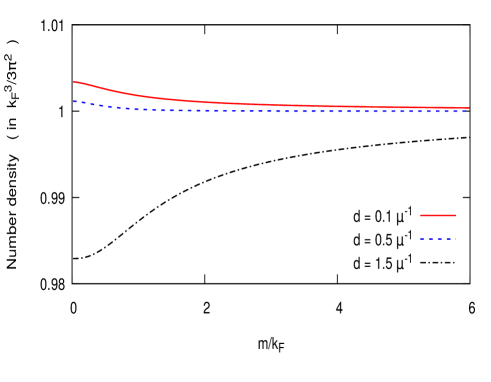
Figure 1: The number density of electrons at zero temperature for different values of length scale $d$.

II.8 Pressure and energy density

Using the expression of pressure for a grand canonical ensemble, we may read off the pressure due to the degenerate electrons as $P_{\psi}=(\beta V)^{-1}\ln\mathcal{Z}_{\psi}$ and due to the interactions as $P_{I}=(\beta V)^{-1}\ln\mathcal{Z}_{I}$. One may check that the radiation pressure $P_{A}=\tfrac{1}{45}\pi^{2}\beta^{-4}$ is insignificant even compared to $P_{I}$, as for white dwarfs $\beta k_{F}\gg 1$. Therefore, by ignoring the radiation component, we can express the total pressure which includes leading order corrections due to the finite temperature and the fine-structure constant, as

$$P=\frac{k_{F}^{4}}{12\pi^{2}}\left[\frac{1+24\sigma_{T}^{2}}{\sigma_{\mu}^{-1}}-\frac{3\sigma^{2}\sigma_{k}^{2}}{2}+\frac{3\alpha}{2\pi}(\sigma_{k}^{4}-\frac{8\pi^{2}d_{+}^{2}n_{e}}{3k_{F}^{3}\sigma_{\mu}^{2}})\right]~{}.$$ (63)

We may again note that the degeneracy pressure depends on the parameter $d_{+}$ which characterizes the electron-nuclei interaction length scale (see Fig. 2).

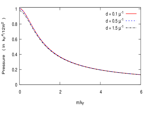
Figure 2: The degeneracy pressure at zero temperature for different values of length scale $d$.

The contribution to the total energy density $\rho$ of the system due to the degenerate electrons can be computed using the formula $(\rho_{e}-\mu n_{e})V=-(\partial\ln\mathcal{Z}/\partial\beta)$ and which is given by

$$\rho_{e}=-P+\mu n_{e}~{}.$$ (64)

For a white dwarf, however, the dominant contribution to the total energy density comes from the contribution of the nuclei, given by

$$\rho_{n}=(A/Z)m_{u}n_{e}~{},$$ (65)

where $A$ is the atomic mass number and $m_{u}$ is the atomic mass unit. For a white dwarf with pure Helium ${}^{4}\mathrm{He}$ core $(A/Z)$ is $2$. Using the Eqs. (62, 63, 65), in principle, one can express the equation of state for the degenerate matter within white dwarfs as $P=P(\rho)$ which includes the corrections due to the fine structure constant $\alpha$ and the finite temperature.

II.9 Non-relativistic limit

We have the considered matter field actions to be manifestly Lorentz invariant here. Consequently the studied equation of state is well suited for describing the relativistic regime. However, for the consistency, the equation of state must also have correct non-relativistic limit when $k_{F}\ll m$. In such limit $\sigma\gg 1$, $\sigma_{\mu}=\sigma+\tfrac{1}{2}\sigma^{-1}-\tfrac{1}{8}\sigma^{-3}+\mathcal{O}(\sigma^{-5})$ and $\sigma_{k}^{2}=\tfrac{2}{3}\sigma^{-1}-\tfrac{1}{5}\sigma^{-3}+\mathcal{O}(\sigma^{-5})$. Therefore, in the non-relativistic regime, the number density (62) reduces to

$$n_{e}\simeq\frac{k_{F}^{3}}{3\pi^{2}}\left[1+\frac{6m^{2}k_{B}^{2}T^{2}}{k_{F}^{4}}+\frac{\alpha(1-d_{+}^{2})k_{F}}{\pi m}\right]~{},$$ (66)

and the pressure (63) reduces to

$$P\simeq\frac{k_{F}^{5}}{15\pi^{2}m}\left[1+\frac{30m^{2}k_{B}^{2}T^{2}}{k_{F}^{4}}+\frac{2\alpha(1-2d_{+}^{2})k_{F}}{3\pi m}\right]~{}.$$ (67)

If one disregards the corrections due to the finite temperature and the fine-structure constant, the Eqs. (66, 67) represent the standard non-relativistic expressions. However, one may note that in the non-relativistic regime the effects of finite temperature become important. Nevertheless, these equations are valid in non-relativistic regime as long as corresponding chemical potential $\mu$ satisfies $\beta\mu\gg 1$.

II.10 Temperature corrections

For non-interacting, zero temperature degenerate electron gas, the number density of electrons is given by $n_{e}=(k_{F}^{3}/3\pi^{2})$. However, the effect of finite temperature causes this relation to be modified even for non-interacting electrons as

$$\frac{n_{e}(T)}{n_{e}(T=0)}=1+\frac{6(2+\sigma^{2})k_{B}^{2}T^{2}}{k_{F}^{2}}~{}.$$ (68)

Analogously, the effect of finite temperature on the pressure of non-interacting degenerate electron gas can be expressed as

$$\frac{P(T)}{P(T=0)}=1+\frac{48\sigma_{\mu}k_{B}^{2}T^{2}}{k_{F}^{2}(2\sigma_{\mu}-3\sigma^{2}\sigma_{k}^{2})}~{}.$$ (69)

Clearly, the finite temperature causes the pressure to increase for a given Fermi momentum $k_{F}$. However, the increase in pressure is very small given it is of the order $\sim(\beta k_{F})^{-2}\sim 10^{-10}$ for typical white dwarfs (1).

II.11 Fine-structure constant corrections

The effects of the electromagnetic interaction i.e. the Coulomb effects on the equation of state are expressed using the fine-structure constant $\alpha\simeq 1/137$ which is a small number. However, theses corrections are much larger compared to the temperature corrections. At the zero temperature, the leading order effect of the fine-structure constant on the electron number density can be expressed as

$$\frac{n_{e}(\alpha)}{n_{e}(\alpha=0)}=1+\frac{\alpha}{2\pi}\left(3\sigma_{k}^{2}-2d_{+}^{2}\sigma_{\mu}^{-1}\right)~{}.$$ (70)

Similarly, at the zero temperature the leading order effect of the fine-structure constant on the pressure can be expressed as

$$\frac{P(\alpha)}{P(\alpha=0)}=1+\frac{\alpha}{3\pi}\frac{(9\sigma_{k}^{4}-8d_{+}^{2}\sigma_{\mu}^{-2})}{(2\sigma_{\mu}-3\sigma^{2}\sigma_{k}^{2})}~{}.$$ (71)

We note that the number density and the pressure both contain an undetermined dimensionless parameter $d_{+}=2d\mu$ in the corrections involving the fine-structure constant. As mentioned earlier, the length scale $d$ is associated with the current-current interaction between the electrons and the nuclei. In the partition function, a natural length scale is provided by the chemical potential $\mu$. Therefore, intuitively one would expect that the dimensionless parameter $d_{+}$ to be an $\mathcal{O}(1)$ number for the white dwarfs. However, determination of its exact numerical values can only be done by using separate considerations, possibly by using observations. In the standard literature, this one-parameter uncertainty is often overlooked as usually there one fixes the lattice scale associated with positively charged nuclei by heuristic arguments. However, we have argued that this length scale is associated with the electron-nuclei interaction and its independent determination in principle can allow one to understand the property of the underlying lattice structure formed by the nuclei within the degenerate matter of the white dwarfs.

II.12 Comparison with Salpeter’s corrections

In order to compare the number density (62) and the pressure (63) with that of Salpeter’s we need to set $\sigma_{T}=0$ as these are studied at zero temperature by Salpeter ¹¹. Further, for comparison we consider the terms up to leading order in fine structure constant $\alpha$ from the combined expressions of non-interacting degeneracy pressure $P_{0}$, classical Coulomb corrections $P_{C}$, Thomas-Fermi corrections $P_{TF}$, exchange corrections $P_{ex}$ and correlation corrections $P_{cor}$ as described in ¹¹.

In the treatment by Salpeter, the relation between the number density of electrons $n_{e}$ and the Fermi momentum $k_{F}$ is assumed to be fixed. On the other hand, the usage of grand canonical partition function here implies that there is a modification to the expression of the electron number density due to the electromagnetic interactions. In turns, it would imply a difference in equation of state even if the pressure expressions considered by Salpeter and here, were to agree.

II.12.1 No interaction

The expressions of the number density (62) and the pressure (63) agree exactly with the Salpeter’s expressions when one ignores the fine-structure constant corrections by setting $\alpha=0$ and identifies $\sigma^{-1}$ as the ‘relativity parameter’ $x$.

II.12.2 Relativistic domain

In the ultra-relativistic limit, $k_{F}\gg m$, we can express the total pressure which includes leading order corrections due to the fine-structure constant, as

$$P=\frac{k_{F}^{4}}{12\pi^{2}}\left[1+\alpha\left(\frac{3}{2\pi}-\frac{4d_{+}^{2}}{3\pi}\right)\right]~{}.$$ (72)

The analogous expression for pressure with leading order corrections considered by Salpeter, can be expressed as $P=\frac{k_{F}^{4}}{12\pi^{2}}\left[1+\alpha(\frac{1}{2\pi}-\frac{6}{5}(\tfrac{4}{9\pi})^{1/3}Z^{2/3})\right]$ ¹¹. Therefore, if one chooses $d_{+}^{2}=\tfrac{3}{4}+(\tfrac{81\pi^{2}}{250})^{1/3}Z^{2/3}$ then one would get the same pressure corrections in the ultra-relativistic limit. In particular, if one chooses the atomic number $Z=2$ (Helium) or $Z=6$ (Carbon) then the Salpeter’s corrections would correspond to the length scale $d$ being $0.88~{}\mu^{-1}$, $1.18~{}\mu^{-1}$ respectively. This is in agreement with the intuitive expectation that $d_{+}$ should be an $\mathcal{O}(1)$ number. The pressure comparison in a broadly relativistic domain is given in the Fig. 3.

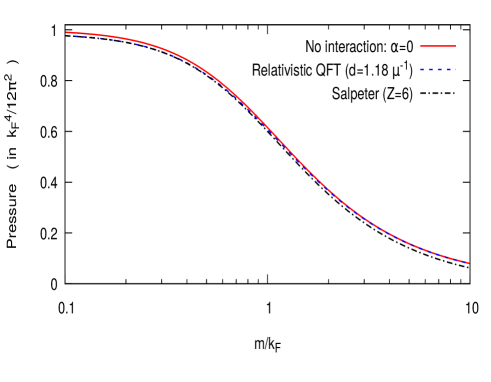
Figure 3: A comparison of the pressure in a broadly relativistic domain.

Nevertheless, we emphasize that the length scale $d$ is undetermined apriori in the approach that we have considered here. For a given system of degenerate electrons and nuclei, in principle, it may be possible to derive an effective action corresponding to Eq. (8) where $\sim d_{+}e$ may be viewed as the renormalized coupling constant between the electrons and the nuclei at the energy scale set by the chemical potential $\mu$.

II.12.3 Non-relativistic domain

The corrections to the pressure expression, considered by Salpeter, are known to become unreliable in a fairly non-relativistic domain. Salpeter noted that with such corrections the total pressure could become negative, signaling the breakdown of the underlying assumptions ¹¹. In contrast, the non-relativistic expression (67) here remains well defined. A comparison of the pressure in a broadly non-relativistic domain is given in the Fig. 4.

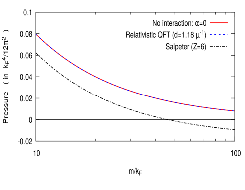
Figure 4: A comparison of the pressure in a broadly non-relativistic domain. The pressure becoming negative signals the breakdown of the underlying assumptions in Salpeter’s treatment.

III Degenerate plasma in curved spacetime

So far we have studied the degenerate plasma by considering the Minkowski spacetime which has vanishing spacetime curvature. In such a set up, the gravitational interaction is incorporated by using the Newtonian gravity. For example, the celebrated Chandrasekhar mass limit for the white dwarfs is derived using the combination of the Newtonian gravity and the equation of state of the degenerate plasma computed in the Minkowski spacetime.

However, the framework of Newtonian gravity is not a very accurate description when the strength of gravitational interaction is strong. On the other hand, Einstein’s general relativity is known to be the most accurate classical description of the gravitational interaction where the gravitation manifests itself through the curvature of the spacetime. Among the compact astrophysical objects, the effect of general relativity for the white dwarfs is relatively smaller. However, the general relativistic effect on a neutron star is quite significant. On the mass-radius relation of these compacts stars, the effects of general relativity appear in two different ways. The first effect arises from the usage of Einstein’s field equations rather than using Poisson’s equation of the Newtonian gravity. The second effect arises due to the effect of curved spacetime on the matter field dynamics and the resultant modifications to the matter EOS due to the gravitational time dilation.

III.1 Tolman-Oppenheimer-Volkoff Equations

In order to include the effects of general relativity in the study of these compact stars, for simplicity, we assume that the spacetime of these stars can be described by a spherically symmetric spacetime geometry. This assumption then leads the exterior vacuum spacetime around these stars to be described by the Schwarzschild solution of Einstein’s equation. On the other hand, in the interior spherical geometry, the invariant line element can be expressed using the natural units, $c=\hbar=1$, as

$$ds^{2}=-e^{2\Phi(r)}dt^{2}+e^{2\nu(r)}dr^{2}+r^{2}(d\theta^{2}+\sin^{2}\theta d\phi^{2})~{},$$ (73)

where $\Phi(r)$ and $\nu(r)$ are the metric functions that are governed by Einstein’s field equations. Further, we assume that the matter stress-energy tensor inside these stars can be treated as a perfect fluid whose expression is given by

$$T^{\mu\nu}=(\rho+P)u^{\mu}u^{\nu}+Pg^{\mu\nu}~{},$$ (74)

where $P$ is the pressure, $\rho$ is the energy density, $g_{\mu\nu}$ is the spacetime metric (73), and $u^{\mu}$ is the 4-velocity of the co-moving observer. The Einstein equations corresponding to the interior metric (73) together with covariant conservation equations of the stress-energy tensor (74) lead to the following set of equations

$$\frac{d\Phi}{dr}=\frac{G(\mathcal{M}+4\pi r^{3}P)}{r(r-2G\mathcal{M})}~{},~{}\frac{dP}{dr}=-(\rho+P)\frac{d\Phi}{dr}~{},$$ (75)

where $\mathcal{M}\equiv\mathcal{M}(r)$, often referred to as the ‘enclosed mass’ upto the radial coordinate $r$, satisfies the equation

$$\frac{d\mathcal{M}}{dr}=4\pi r^{2}\rho~{}.$$ (76)

These equations (75, 76) govern the matter distribution inside the spherical stars and are known as the Tolman-Oppenheimer-Volkoff (TOV) equations. In the limit where the speed of light $c\rightarrow\infty$, the TOV eqs. lead to the Poisson equation of the Newtonian gravity. The other metric function $\nu(r)$ can be partially solved and can be expressed as

$$e^{-2\nu(r)}=1-\frac{2G\mathcal{M}}{r}~{}.$$ (77)

In order to solve the TOV equations where there are three independent equations (75, 76) but four unknown functions, namely $\mathcal{M}$, $\Phi$, $P$ and $\rho$, one needs to provide the matter equation of state of the form $P=P(\rho)$. However, being nonlinear in nature, these equations cannot be solved analytically for a given matter EOS. Therefore, in order to compute the resultant mass-radius relations of these compact stars, one needs to deploy numerical methods for solving the TOV equations.

III.2 Effect of gravitational time dilation on EOS

The second kind of general relativistic effect that arises in the study of compact astrophysical objects, is the effect of gravitational time dilation on the matter EOS. In the literature, this effect is often overlooked. In the general relativity, any curved spacetime can be described locally by a flat metric. This argument is then used to deploy a matter EOS computed in a globally flat spacetime, here referred to as the flat EOS, for solving the TOV equations. However, such a argument misses the fact that inside the star, the metric function $\Phi$ varies radially over the scale of the star, as governed by the eq. (75). Therefore, two locally inertial frames which are located at different radial locations have different lapse functions and consequently have different clock speeds.

By using a first-principle approach, the effect of gravitational time dilation on the matter EOS has been computed for different types of degenerate matter ^{30, 31}. Here we follow a simpler approach by suitably transforming the quantities computed in a globally flat spacetime, as prescribed in the ref. ³⁰. We would like to emphasize here that in this context two different scales are involved. Firstly, at the scale of local thermodynamical equilibrium, the thermodynamical quantities such as the pressure and the energy density are uniform. In this scale, the metric function $\Phi$ must also be considered as uniform. For definiteness, let us consider a small box whose center is located at a radial coordinate $r_{0}$, so that local thermodynamical equilibrium holds within the box. For a spherical star, one can always define a local set of coordinates as $\tilde{X}=e^{\nu(r_{0})}r\sin\bar{\theta}\cos\phi$, $\tilde{Y}=e^{\nu(r_{0})}r\sin\bar{\theta}\sin\phi$, and $\tilde{Z}=e^{\nu(r_{0})}r\cos\bar{\theta}$ where $\bar{\theta}=e^{-\nu(r_{0})}\theta$ such that the metric (73) inside the box can be written as ³⁰

$$ds^{2}=-e^{2\Phi(r_{0})}dt^{2}+d\tilde{X}^{2}+d\tilde{Y}^{2}+d\tilde{Z}^{2}~{}.$$ (78)

One may now use the locally flat coordinate system $(t,\tilde{X},\tilde{Y},\tilde{Z})$ within the box to compute the matter EOS within the box where the metric function $\Phi\equiv\Phi(r_{0})$ has a fixed value. This computation leads the matter EOS to retain its dependence on the metric function $\Phi$. Subsequently, such an EOS, referred to as the curved EOS, can be used to solve the TOV equations. Nevertheless, it is possible to obtain the corresponding curved EOS starting from the partition function computed in a globally flat spacetime. We note that if one defines a new time coordinate as $\tilde{t}=e^{\Phi}t$ within the box then the metric in the coordinate system $(\tilde{t},\tilde{X},\tilde{Y},\tilde{Z})$ becomes the same as the Minkowski metric. At thermodynamical equilibrium, the anti-periodic boundary condition (14) then leads to the following relations ³⁰

$$\tilde{\beta}=\beta e^{\Phi}~{}~{},~{}~{}\tilde{\mu}=\mu e^{-\Phi}~{},$$ (79)

where $\tilde{\beta}=1/(k_{B}\tilde{T})$ with $\tilde{T}$ and $\tilde{\mu}$ being the temperature and chemical potential respectively, as seen in the frame $(\tilde{t},\tilde{X},\tilde{Y},\tilde{Z})$. Using the transformations (79) and by ignoring the contributions coming from the electromagnetic interactions, the partition function for degenerate electrons (18) within the box becomes

$$\ln\mathcal{Z}_{\psi}=\frac{\beta Ve^{-3\Phi}}{24\pi^{2}}\left[2\mu\mu_{m}^{3}-3\bar{m}^{2}\bar{\mu}_{m}^{2}+\frac{48\mu\mu_{m}}{\beta^{2}}\right]~{},$$ (80)

where $\mu_{m}\equiv\sqrt{\mu^{2}-\bar{m}^{2}}$, $\bar{\mu}_{m}^{2}\equiv\mu\mu_{m}-\bar{m}^{2}\ln(\tfrac{\mu+\mu_{m}}{\bar{m}})$ and $\bar{m}=me^{\Phi}$. Here we have expressed the partition function in terms of the chemical potential $\mu$, as $\mu$ is independent of the choice of spatial coordinates, unlike the Fermi momentum $k_{F}$.

By using the expression of the partition function (80) for degenerate electrons, the expressions for the number density $n_{e}$, the pressure $P$ and the energy density $\rho_{e}$ can be derived explicitly as $n_{e}=(\beta V)^{-1}(\partial\ln\mathcal{Z}_{\psi}/\partial\mu)$, $P=(\beta V)^{-1}\ln\mathcal{Z}_{\psi}$, and $(\rho_{e}-\mu n_{e})V=-(\partial\ln\mathcal{Z}_{\psi}/\partial\beta)$. The expressions for the pressure and the energy density then can be written as

$$P =e^{\Phi}\frac{m^{4}}{24\pi^{2}}\Big{[}\sqrt{(bn_{e})^{2/3}+1}\left\{2(bn_{e})-3(bn_{e})^{1/3}\right\}$$

$$+3\operatorname{asinh}((bn_{e})^{1/3})\Big{]}~{},~{}$$ (81)

and

$$\rho_{e}=-P+e^{\Phi}\frac{m^{4}}{3\pi^{2}}\sqrt{(bn_{e})^{2/3}+1}~{}(bn_{e})~{},$$ (82)

where $b=(3\pi^{2}/m^{3})(Z/A)$. On the other hand, in the curved spacetime the expression of the energy density of the nuclei becomes

$$\rho_{n}=(A/Z)m_{u}n_{e}e^{\Phi}~{},$$ (83)

when one includes the effect of gravitational time dilation ³⁰. We note that in the eqs. (III.2, 82, 83) if one turns off the gravitational time dilation effect by setting $e^{\Phi}\to 1$, then the expressions of the pressure and the energy density derived in curved spacetime reduce to their Minkowski spacetime counterparts (63, 64, 65) without the corrections from the electromagnetic interactions.

IV White dwarfs

In this section, we discuss a few consequences of using the equation of state of the degenerate plasma which is computed using the thermal field theory approach, for the white dwarfs. The expression for the degeneracy pressure which is relevant for the white dwarfs, is obtained in eq. (63) for the flat spacetime and in the eq. (III.2) for the curved spacetime but without the fine-structure constant corrections. On the other hand, the expressions for the relevant mass-energy density, obtained by considering the appropriate number of nuclei present within the white dwarfs to ensure overall $U(1)$ charge neutrality, are given in the eqs. (65, 83).

IV.1 Modified mass limit of white dwarfs

The usage of the Newtonian gravity together with the equation of state computed in the Minkowski spacetime leads to a maximum mass of a white dwarf, known as the Chandrasekhar mass limit. Without the fine-structure constant corrections, this mass limit can be expressed as $M^{0}_{ch}=(4/\sqrt{\pi})(\mathrm{K}_{0}/G)^{3/2}|\xi_{0}^{2}~{}\theta^{\prime}(\xi_{0})|$ where $K_{0}$ is known as the polytropic constant, given by

$$\mathrm{K}_{0}=\frac{(3\pi^{2})^{1/3}}{4((A/Z)m_{u})^{4/3}}~{}.$$ (84)

Here $\theta$ is the solution of the Lane-Emden equation $\xi^{-2}\tfrac{d}{d\xi}\left(\xi^{2}\frac{d\theta}{d\xi}\right)=-\theta^{3}$ and $\xi_{0}$ is the point where $\theta(\xi_{0})$ vanishes first. By solving the Lane-Emden equation numerically, one obtains $|\xi_{0}^{2}~{}\theta^{\prime}(\xi_{0})|\simeq 2.02$.

In order to obtain the effect of the fine-structure constant on the Chandrasekhar mass limit, we need to find the corrections to the equation of state in the ultra-relativistic limit. In such limit, the eqs. (62, 63, 65) together lead to a polytropic equation of state of the form $P\propto\rho^{4/3}$ where fine-structure constant modifies the proportionality constant. Such a modification in turn leads to the modified Chandrasekhar mass limit $M_{ch}$ which including up to the leading order correction in the fine-structure constant $\alpha$, is given by ³²

$$\frac{M_{ch}}{M^{0}_{ch}}=1-\frac{3\alpha}{4\pi}~{}.$$ (85)

We note that the effect of the fine-structure constant $\alpha$ reduces the Chandrasekhar mass limit for white dwarfs by a universal factor ³². In particular, the length scale $d$ which is associated with the electron-nuclei interaction, does not affect the mass limit for the white dwarfs. In contrast, the modified Chandrasekhar mass limit which uses the Salpeter’s corrections, can be expressed up to leading order in $\alpha$, as $M_{ch}/M^{0}_{ch}=1-\frac{3}{2}\alpha\left[\frac{6}{5}(\tfrac{4}{9\pi})^{1/3}Z^{2/3}-\tfrac{1}{2\pi}\right]$ ^{13, 11, 12}. So there the reduction of the Chandrasekhar mass limit is non-universal in nature as it depends on the atomic number of the constituent nuclei.

IV.2 Mass radius relations

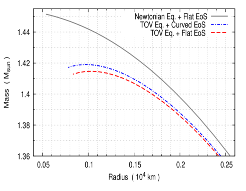
Figure 5: Comparison of mass radius relations of the white dwarfs in the Newtonian gravity and the general relativity without the corrections involving the fine-structure constant.

In order to obtain the mass-radius relations of the white dwarfs that includes modifications from the general relativity, the TOV eqs. (75, 76) needs to be solved numerically. For the white dwarfs, the dominant contribution to energy density comes from the nuclei. In a computation based on a globally flat spacetime, the energy density due to the nuclei is given by the eq. (65). On the other hand, in a curved spacetime the expression of the energy density due to the nuclei is given in the eq. (83) which includes the effect of gravitational time dilation. By ignoring the corrections due to the fine-structure constant but including two different effects from the general relativity, the resultant mass-radius relations for the white dwarfs are plotted in the Fig. 5. We note that the maximum mass of the white dwarfs reduces by around $2.4\%$ due to the usage of the TOV eqs. compared to the same of the Newtonian gravity. On the other hand, the inclusion of the time dilation effect into the matter EOS leads to an increase of the maximum mass by around $0.7\%$.

V Neutron stars

Unlike the case of white dwarfs, the effect of general relativity on the neutron stars is significant. It is essentially due to the fact that the neutron stars are among the most compact astrophysical objects that can be observed directly. Such a compact yet massive object curves the spacetime around it very strongly. Besides, it requires its interior energy density to be order of the nuclear density. Unfortunately, the physical understanding of such a dense nuclear matter plasma is still an active area of research. Consequently, several models of the equation of states for the neutron stars have been studied in the literature.

V.1 Mass radius relations

The simplest model of the plasma contained within the neutron stars consists of an ensemble of non-interacting degenerate neutrons. The relevant equation of state can be obtained from the eqs. (III.2, 82) by mapping the mass of electrons to the mass of neutrons and by setting $(Z/A)=1$. The corresponding TOV eqs. then can be solved using the numerical methods. The resultant mass-radius relations for such an ideal neutron star are plotted in the Fig. 6 for both the curved EOS and the flat EOS ³⁰. The curved EOS leads to a significant increase in the mass of neutron stars for a given radius. In particular, the maximum mass of the ideal neutron stars increases by around $16.9\%$ whereas its corresponding radius increases by around $2.2\%$.

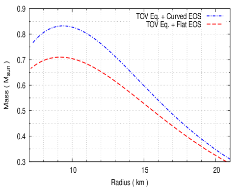
Figure 6: Mass radius relations of the ideal neutron stars using both the curved EOS and the flat EOS.

Nevertheless, it is quite clear from the Fig. 6, that the simplest model of equation of state for the neutron stars can not explain the observations of astrophysical neutron stars having mass even more than $2M_{\odot}$ ^{33, 34}. In order to explain such high masses of the neutron stars, one often consider the models of equation of state of neutron stars where the nuclear plasmas are made of interacting nucleons. In the framework of quantum hadrodynamics ^{35, 36}, one such model to describe the nuclear matter within the neutron stars is known as the so-called $\sigma-\omega$ model ^{37, 38, 39}. By considering a $\sigma-\omega$ model having two baryons, namely the neutron and the proton, a lepton namely the electron, a massive scalar meson $\sigma$ and a self-interacting vector meson $\omega$, both the flat EOS and the curved EOS for the neutron stars have been computed in ³¹. The corresponding mass-radius relations of the neutron stars are shown in the Fig. 7. The effect of gravitational time dilation on EOS leads to a significant increase in the maximum mass of neutron stars. In particular, here the maximum mass of the neutron stars increases almost by $39.1\%$, and its corresponding radius increases by almost $29.8\%$ for a given set of parameters of the $\sigma-\omega$ model.

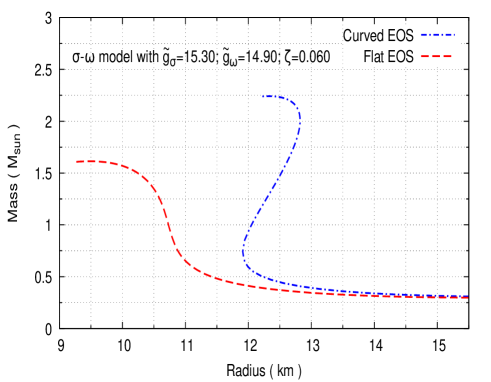
Figure 7: Mass radius relations of the neutron stars in the $\sigma-\omega$ model using both the curved EOS and flat EOS for a given set of parameter values.

VI Discussions

In summary, in this review, we have employed the methods of relativistic thermal quantum field theory to compute the equation of states of degenerate plasmas contained within the compact astrophysical objects such as the white dwarfs and the neutron stars. In particular, we have computed these equation of states including leading order corrections due to the finite temperature, due to the electromagnetic interactions, parameterized by the fine-structure constant, as well as the effect of gravitational time dilation. In the literature, the effects of the electromagnetic interaction on the equation of state of the degenerate matter within the white dwarfs are computed by considering the so-called classical Coulomb energy, the Thomas-Fermi effect, the exchange and correlation energy at zero temperature. These computations rely on the electrostatic considerations which are non-relativistic ab initio. After reviewing the existing treatments in the literature, here we have presented the computation of the equation of states of degenerate matter for the white dwarfs by employing the methods of thermal quantum field theory which is a relativistic approach ab-initio. The resultant correction to the equation of state due to the fine-structure constant has two components. The first component arises from the self-interaction between the degenerate electrons and described by the action of quantum electrodynamics. For the second component we have considered a Lorentz invariant interaction term to describe the interaction between the electrons and the positively charged nuclei. Further, we have argued that a fully relativistic consideration leads to an apriori undetermined length scale in the corrections to the equation of state involving the electron-nuclei interaction. This aspect of the equation state is overlooked in the literature. Instead there one fixes the associated scale by using heuristic arguments. An independent determination of this length scale may shed light on the underlying lattice structure formed by the nuclei within the degenerate matter of the white dwarfs. Besides, the effect of fine-structure constant reduces the Chandrasekhar mass limit of the white dwarfs by a universal factor which is independent of the atomic number of the constituent nuclei and the electron-nuclei interaction length scale.

In order to include the effects of general relativity in the equation of states of the degenerate plasmas, here we have considered the spacetime of these compact stars to be described by a spherically symmetric spacetime geometry. We have shown that the effects of general relativity on the mass radius relation of the compacts stars appear in two different ways. The first kind of effect arises from the usage of Einstein’s field equations rather than using the Poisson’s equation of Newtonian gravity. The second kind of effect arises due to the effect of gravitational time dilation on matter field dynamics and the resultant modifications to the matter equation of state. Among the compact astrophysical objects, the effect of general relativity is relatively smaller for the white dwarfs. However, the general relativistic effect on the neutron stars is quite significant.

In this review, we have primarily considered the system of plasmas within the astrophysical compacts stars. However, in principle, the field theoretical description of the plasmas that are studied here, can also be applied for a earth-based plasma system as long as the degeneracy condition $\beta\mu\gg 1$ can be satisfied. For examples, if one is dealing with the plasmas having temperature $10^{4}$ K and if the associated chemical potential $\mu$ is $100~{}eV$ then $\beta\mu>10^{2}$ where the description as studied here would be equally applicable.

Finally, we note that the observations of gravitational waves originating from coalescence events involving neutron stars, by the current ground-based gravitational wave detectors have already started putting severe constraints on the equation of states of the degenerate plasmas present within the neutron stars ^{40, 41, 42, 43}. Furthermore, future detection of low-frequency gravitational waves from the extreme mass-ratio merger of a black hole and a white dwarf could determine the equation of state of the degenerate matter within the white dwarf with an accuracy reaching up to $0.1\%$ ²². It is based on the expectation that the tidal disruption of a white dwarf, during the final phase of inspiral around a massive black hole, could be measured very accurately through low-frequency gravitational wave signals. The properties of the tidal disruption of a white dwarf would necessarily depend on the equation of state of the degenerate matter present within the white dwarf. On the other hand, we may note from the Eqs. (70, 71) that the corrections to the number density and the pressure due to the fine-structure constant are of the order $\sim\alpha/\pi\sim 0.2\%$. Therefore, the effects of the fine-structure constant as studied here could well be within the detection realm of the future gravitational wave detectors. We may mention here that the deviation of equation of state compared to that of Salpeter’s equation of state for white dwarf is relatively larger in the non-relativistic regime, as can be seen in the Fig. 4. Clearly, such deviations can be confronted with the expected accuracy of the future low-frequency gravitational wave detectors.

VII Acknowledgments

SM would like to thank IISER Kolkata for supporting this work through a doctoral fellowship.

References

- Abbott et al. [2016] Abbott BP, Abbott R, Abbott T, Abernathy M, Acernese F, Ackley K, Adams C, Adams T, Addesso P, Adhikari R, et al. (2016) Observation of gravitational waves from a binary black hole merger. Physical review letters 116(6):061102
- Abbott et al. [2017] Abbott BP, Abbott R, Abbott T, Acernese F, Ackley K, Adams C, Adams T, Addesso P, Adhikari R, Adya V, et al. (2017) Gw170817: observation of gravitational waves from a binary neutron star inspiral. Physical review letters 119(16):161101
- Shaddock [2008] Shaddock D (2008) Space-based gravitational wave detection with lisa. Classical and Quantum Gravity 25(11):114012
- Hulse and Taylor [1975] Hulse RA, Taylor JH (1975) Discovery of a pulsar in a binary system. The Astrophysical Journal 195:L51–L53
- Taylor and Weisberg [1989] Taylor JH, Weisberg JM (1989) Further experimental tests of relativistic gravity using the binary pulsar psr 1913+ 16. The Astrophysical Journal 345:434–450
- Chandrasekhar [1931] S. Chandrasekhar, The Astrophysical Journal 74, 81 (1931).
- Chandrasekhar [1935] S. Chandrasekhar, Monthly Notices of the Royal Astronomical Society 95, 207 (1935).
- Frenkel [1928] J. Frenkel, Zeitschrift fur Physik 50, pp. 234–248 (1928).
- Kothari [1938] D. Kothari, Proceedings of the Royal Society of London. Series A, Mathematical and Physical Sciences pp. 486–500 (1938).
- Auluck and Mathur [1959] F. Auluck and V. Mathur, Zeitschrift fur Astrophysik 48, 28 (1959).
- Salpeter [1961] E. E. Salpeter, The Astrophysical Journal 134, 669 (1961).
- Hamada and Salpeter [1961] T. Hamada and E. Salpeter, The Astrophysical Journal 134, 683 (1961).
- Nauenberg [1972] M. Nauenberg, The Astrophysical Journal 175, 417 (1972).
- Koester and Chanmugam [1990] D. Koester and G. Chanmugam, Reports on Progress in Physics 53, 837 (1990).
- Stuart L. Shapiro [1983] S. A. T. Stuart L. Shapiro, Black holes, white dwarfs, and neutron stars: the physics of compact objects (Wiley, 1983), 1st ed.
- Rotondo et al. [2011a] M. Rotondo, J. A. Rueda, R. Ruffini, and S.-S. Xue, Phys. Rev. C 83, 045805 (2011a).
- Rotondo et al. [2011b] M. Rotondo, J. A. Rueda, R. Ruffini, and S.-S. Xue, Phys. Rev. D 84, 084007 (2011b).
- de Carvalho et al. [2014] S. M. de Carvalho, M. Rotondo, J. A. Rueda, and R. Ruffini, Phys. Rev. C 89, 015801 (2014).
- Kovetz and Shaviv [1970] A. Kovetz and G. Shaviv, Astronomy and Astrophysics 8, 398 (1970).
- Shaviv and Kovetz [1972] G. Shaviv and A. Kovetz, Astronomy and Astrophysics 16, 72 (1972).
- Fantoni [2017] R. Fantoni, J. Stat. Mech. 1711, 113101 (2017), eprint arXiv:1709.06064.
- Han and Fan [2018] W.-B. Han and X.-L. Fan, Astrophys. J. 856, 82 (2018), eprint arXiv:1711.08628.
- Matsubara [1955] T. Matsubara, Progress of theoretical physics 14, 351 (1955).
- Akhiezer and Peletminskii [1960] I. Akhiezer and S. Peletminskii, Zh. Eksp. Teor. Fiz. 11, 1316 (1960).
- Freedman and McLerran [1977] B. A. Freedman and L. D. McLerran, Phys. Rev. D 16, 1147 (1977).
- Joyce et al. [2018] S. R. G. Joyce, M. A. Barstow, J. B. Holberg, H. E. Bond, S. L. Casewell, and M. R. Burleigh, Monthly Notices of the Royal Astronomical Society 481, 2361 (2018), eprint arXiv:1809.01240.
- Joseph I. Kapusta [2006] C. G. Joseph I. Kapusta, Finite-Temperature Field Theory: Principles and Applications, Cambridge Monographs on Mathematical Physics (Cambridge University Press, 2006), 2nd ed.
- Weinberg [1995] S. Weinberg, Quantum theory of fields. Foundations, vol. Volume 1 (Cambridge University Press, 1995), 1st ed.
- Nair [2005] V. P. Nair, Quantum Field Theory: A Modern Perspective, Graduate Texts in Contemporary Physics (Springer, 2005), 1st ed.
- Hossain and Mandal [2021] G. M. Hossain and S. Mandal, Journal of Cosmology and Astroparticle Physics 2021, 026 (2021).
- Hossain and Mandal [2021] Hossain GM, Mandal S (2021) Higher mass limits of neutron stars from the equation of states in curved spacetime. arXiv:2109.09606
- Hossain and Mandal [2019] G. M. Hossain and S. Mandal (2019), eprint arXiv:1904.09779.
- Linares et al. [2018] M. Linares, T. Shahbaz, and J. Casares, The Astrophysical Journal 859, 54 (2018).
- Cromartie et al. [2020] H. T. Cromartie, E. Fonseca, S. M. Ransom, P. B. Demorest, Z. Arzoumanian, H. Blumer, P. R. Brook, M. E. DeCesar, T. Dolch, J. A. Ellis, et al., Nature Astronomy 4, 72 (2020).
- Serot [1992] B. D. Serot, Reports on Progress in Physics 55, 1855 (1992).
- Serot and Walecka [1997] B. D. Serot and J. D. Walecka, International Journal of Modern Physics E 6, 515 (1997).
- Whittenbury et al. [2014] D. Whittenbury, J. Carroll, A. Thomas, K. Tsushima, and J. Stone, Physical Review C 89, 065801 (2014).
- Katayama et al. [2012] T. Katayama, T. Miyatsu, and K. Saito, The Astrophysical Journal Supplement Series 203, 22 (2012).
- Miyatsu et al. [2013] T. Miyatsu, S. Yamamuro, and K. Nakazato, The Astrophysical Journal 777, 4 (2013).
- Zhang and Li [2019] Zhang NB, Li BA (2019) Extracting nuclear symmetry energies at high densities from observations of neutron stars and gravitational waves. The European Physical Journal A 55(3):1–23
- Lackey et al. [2006] Lackey BD, Nayyar M, Owen BJ (2006) Observational constraints on hyperons in neutron stars. Physical Review D 73(2):024021
- Takami et al. [2014] Takami K, Rezzolla L, Baiotti L (2014) Constraining the equation of state of neutron stars from binary mergers. Physical Review Letters 113(9):091104
- Chatziioannou [2020] Chatziioannou K (2020) Neutron-star tidal deformability and equation-of-state constraints. General Relativity and Gravitation 52(11):1–49