Conserved currents and $\text{T}\bar{\text{T}}_{s}$ irrelevant deformations of 2D integrable field theories

Abstract

It has been recently discovered that the $\text{T}\bar{\text{T}}$ deformation is closely-related to Jackiw-Teitelboim gravity. At classical level, the introduction of this perturbation induces an interaction between the stress-energy tensor and space-time and the deformed EoMs can be mapped, through a field-dependent change of coordinates, onto the corresponding undeformed ones. The effect of this perturbation on the quantum spectrum is non-perturbatively described by an inhomogeneous Burgers equation. In this paper, we point out that there exist infinite families of models where the geometry couples instead to generic combinations of local conserved currents labelled by the Lorentz spin. In spirit, these generalisations are similar to the $\text{J}\bar{\text{T}}$ model as the resulting theories and the corresponding scattering phase factors are not Lorentz invariant. The link with the $\text{J}\bar{\text{T}}$ model is discussed in detail. While the classical setup described here is very general, we shall use the sine-Gordon model and its CFT limit as explanatory quantum examples. Most of the final equations and considerations are, however, of broader validity or easily generalisable to more complicated systems.

1 Introduction

The deformation of 2D quantum field theories Smirnov:2016lqw ; Cavaglia:2016oda by the Zamolodchikov’s $\text{T}\bar{\text{T}}$ operator Zamolodchikov:2004ce , has recently attracted the attention of theoretical physicists due to the many important links with effective string theory Dubovsky:2012wk ; dubovsky2012effective ; Caselle:2013dra ; Chen:2018keo and the AdS/CFT correspondence McGough:2016lol ; Turiaci:2017zwd ; Giveon:2017nie ; Giveon:2017myj ; Asrat:2017tzd ; Giribet:2017imm ; Kraus:2018xrn ; Cottrell:2018skz ; Baggio:2018gct ; Babaro:2018cmq . A remarkable property of this perturbation, discovered in Smirnov:2016lqw ; Cavaglia:2016oda , concerns the evolution of the quantum spectrum at finite volume $R$, with periodic boundary conditions, in terms of the $\text{T}\bar{\text{T}}$ coupling constant $\tau$. The spectrum is governed by the hydrodynamic-type equation

$$\partial_{\tau}E(R,\tau)=\frac{1}{2}\partial_{R}\left(E^{2}(R,\tau)-P^{2}(R)\right)\;,$$ (1)

where $E(R,\tau)$ and $P(R)$ are the eigenvalues of the energy and momentum operator, respectively, on a generic eigenstate $|n\rangle$. Important for the current purposes is that, under the perturbation, the evolution of the spectrum is equivalently encoded in the following Lorentz-type transformation

$$\left(\begin{array}[]{c}E(R,\tau)\\ P(R)\end{array}\right)=\left(\begin{array}[]{cc}\cosh{(\theta_{0})}&\sinh{(\theta_{0})}\\ \sinh{(\theta_{0})}&\cosh{(\theta_{0})}\end{array}\right)\left(\begin{array}[]{c}E(\mathcal{R}_{0})\\ P(\mathcal{R}_{0})\end{array}\right)\;,$$ (2)

with $\mathcal{R}_{0}$ and $\theta_{0}$ defined through

$$\sinh{\theta_{0}}=\frac{\tau\,P(R)}{\mathcal{R}_{0}}=\frac{\tau\,P(\mathcal{R}_{0})}{R}\;,\quad\cosh{\theta_{0}}=\frac{R+\tau\,E(R,\tau)}{\mathcal{R}_{0}}=\frac{\mathcal{R}_{0}-\tau\,E(\mathcal{R}_{0})}{R}\;.$$ (3)

From (2), it follows that the solution to (1) can be written, in implicit form, as

$$E^{2}(R,\tau)-P^{2}(R)=E^{2}(\mathcal{R}_{0})-P^{2}(\mathcal{R}_{0})\;,$$ (4)

with the additional constraint

$$\partial_{\tau}R=-E(R,\tau)\;,$$ (5)

at fixed $\mathcal{R}_{0}$, obtainable directly from (3) (cf. with the $s=1$ case of (4.2)).
As extensively discussed in Conti:2018tca (see also Dubovsky:2017cnj ), the solutions to the classical EoMs associated to the $\text{T}\bar{\text{T}}$-deformed Lagrangians Cavaglia:2016oda ; Bonelli:2018kik ; Conti:2018jho ; Conti:2018tca are obtained from the $\tau=0$ ones by a field-dependent coordinate transformation

$$dx^{\mu}=\left(\delta^{\mu}_{\;\;\nu}+\tau\,\widetilde{\bm{T}}^{\mu}_{\;\;\nu}(\mathbf{y})\right)dy^{\nu}\;,\quad\mathbf{y}=(y^{1},y^{2})=(x^{\prime},t^{\prime})\;,$$ (6)

with

$$\widetilde{\bm{T}}^{\mu}_{\;\;\nu}(\mathbf{y})=-g^{\mu\delta}\epsilon_{\delta\rho}\,\epsilon_{\sigma\nu}\,{\bm{T}}^{\rho\sigma}(\mathbf{y})\;,\quad\epsilon_{\mu\nu}=\left(\begin{array}[]{cc}0&1\\ -1&0\end{array}\right)_{\mu\nu}\;,$$ (7)

where ${\bm{T}}^{\mu\nu}(\mathbf{y})$ is the Hilbert stress-energy tensor associated to the undeformed theory, canonically defined as

$${\bm{T}}^{\mu\nu}(\mathbf{y})=\frac{-2}{\sqrt{g}}\frac{\partial\mathcal{L}_{g}(\mathbf{y})}{\partial g_{\mu\nu}}\;,\quad\sqrt{g}=\sqrt{\det{(g_{\mu\nu})}}\;,$$ (8)

and $\mathcal{L}_{g}(\mathbf{y})$ is the undeformed Lagrangian in the set of cartesian coordinates $\mathbf{y}$, minimally coupled to gravity through the metric $g_{\mu\nu}$. As shown in Conti:2018tca , equation (6) can be inverted as

$$dy^{\mu} = \left(\delta^{\mu}_{\;\;\nu}-\tau\,\widetilde{\bm{T}}^{\mu}_{\;\;\nu}(\mathbf{x},\tau)\right)dx^{\nu}\;,\quad\mathbf{x}=(x^{1},x^{2})=(x,t)\;,$$ (9)

with

$$\widetilde{\bm{T}}^{\mu}_{\;\;\nu}(\mathbf{x},\tau)=-g^{\mu\delta}\epsilon_{\delta\rho}\,\epsilon_{\sigma\nu}\,{\bm{T}}^{\rho\sigma}(\mathbf{x},\tau)\;,$$ (10)

where ${\bm{T}}^{\mu\nu}(\mathbf{x},\tau)$ is now the Hilbert stress-energy tensor associated to the $\text{T}\bar{\text{T}}$-deformed theory

$$T^{\mu\nu}(\mathbf{x},\tau)=\frac{-2}{\sqrt{g}}\frac{\partial\mathcal{L}_{g}(\mathbf{x},\tau)}{\partial g_{\mu\nu}}\;,$$ (11)

and $\mathcal{L}_{g}(\mathbf{x},\tau)$ is the deformed Lagrangian in the set of cartesian coordinates $\mathbf{x}$. Following the convention of Conti:2018tca , we will switch from cartesian to complex coordinates according to

$$\begin{cases}z=x^{1}+i\,x^{2}\\ \bar{z}=x^{1}-i\,x^{2}\end{cases}\;,\quad\begin{cases}w=y^{1}+i\,y^{2}\\ \bar{w}=y^{1}-i\,y^{2}\end{cases}\;,$$ (12)

and we shall denote with $\mathbf{z}=(z,\bar{z})$ and $\mathbf{w}=(w,\bar{w})$ the two set of complex coordinates.
An important link with topological gravity was noticed and studied in Dubovsky:2017cnj , where it was shown that JT gravity coupled to matter leads to a scattering phase matching that associated to the $\text{T}\bar{\text{T}}$ perturbation Dubovsky:2012wk ; dubovsky2012effective ; Caselle:2013dra ; Smirnov:2016lqw ; Cavaglia:2016oda . Equations (6) and (9) were also obtained in Conti:2018tca starting from the deformed EoMs following, therefore, a completely independent line of thoughts compared to Dubovsky:2017cnj . However, the final results turn out to be fully consistent with the proposal of Dubovsky:2017cnj . In this paper, we shall argue that the approach of Conti:2018tca admits natural generalisations corresponding to infinite families of geometric-type deformations of classical and quantum field theories.
Our analysis starts from (6) and the observation that the equality between the second mixed derivatives implies

$$\frac{\partial^{2}x^{\mu}}{\partial y^{\rho}\partial y^{\sigma}}=\frac{\partial^{2}x^{\mu}}{\partial y^{\sigma}\partial y^{\rho}}\quad\Longleftrightarrow\quad\partial_{\mu}{\bm{T}}^{\mu\nu}=0\;.$$ (13)

Equation (13) suggests that a consistent and natural generalisation of (6) can be obtained by replacing the stress-energy tensor with an arbitrary (rank-two) conserved current. Thus, the main objective of this work is to study the generalisations of the change of coordinates (6) obtained by replacing ${\bm{T}}^{\mu\nu}$ with a matrix built using the higher-spin conserved currents, typically present in free or integrable theories. In complex coordinates $\mathbf{z}$, the spin ${\bf{s}}$ conserved currents ${\bf T}_{{\bf{s}}+1}$, ${\bf\bar{T}}_{{\bf{s}}+1}$, ${\bf\Theta}_{{\bf{s}}-1}$ and ${\bf\bar{\Theta}}_{{\bf{s}}-1}$ are related through the continuity equations

$$\bar{\partial}{\bf T}_{{\bf{s}}+1}=\partial{\bf\Theta}_{{\bf{s}}-1}\;,\quad\partial{\bf\bar{T}}_{{\bf{s}}+1}=\bar{\partial}{\bf\bar{\Theta}}_{{\bf{s}}-1}\;,\quad({\bf{s}}\in{\mathbb{N}})\;,$$ (14)

where $\partial=\partial_{z}$ and $\bar{\partial}=\partial_{\bar{z}}$, the subscripts ${\bf{s}}+1$ and ${\bf{s}}-1$ are the Lorentz spins of the corresponding field and the ${\bf{s}}=1$ case of (14) corresponds to the energy and momentum conservation law. The replacement we shall perform in (6)–(7) is

$${\bm{T}}\quad\longrightarrow\quad{\bm{T}}_{\bf{s}}\;,$$ (15)

where the cartesian and complex components of ${\bm{T}}_{\bf{s}}$ are related through

$$({\bm{T}}_{\bf{s}})_{11}=-\frac{1}{2\pi}\left({\bf\bar{T}}_{{\bf{s}}+1}+{\bf T}_{{\bf{s}}+1}-{\bf\bar{\Theta}}_{{\bf{s}}-1}-{\bf\Theta}_{{\bf{s}}-1}\right) ({\bm{T}}_{\bf{s}})_{12}=\frac{i}{2\pi}\left({\bf\bar{T}}_{{\bf{s}}+1}-{\bf T}_{{\bf{s}}+1}+{\bf\bar{\Theta}}_{{\bf{s}}-1}-{\bf\Theta}_{{\bf{s}}-1}\right),$$ ,

$$({\bm{T}}_{\bf{s}})_{21}=\frac{i}{2\pi}\left({\bf\bar{T}}_{{\bf{s}}+1}-{\bf T}_{{\bf{s}}+1}-{\bf\bar{\Theta}}_{{\bf{s}}-1}+{\bf\Theta}_{{\bf{s}}-1}\right) ({\bm{T}}_{\bf{s}})_{22}=\frac{1}{2\pi}\left({\bf\bar{T}}_{{\bf{s}}+1}+{\bf T}_{{\bf{s}}+1}+{\bf\bar{\Theta}}_{{\bf{s}}-1}+{\bf\Theta}_{{\bf{s}}-1}\right).$$ ,

For simplicity, it will be useful to define the re-scaled quantities

$${\rm T}_{{\bf{s}}+1}=\frac{{\bf T}_{{\bf{s}}+1}}{2\pi}\;,\quad\Theta_{{\bf{s}}-1}=\frac{{\bf\Theta}_{{\bf{s}}-1}}{2\pi}\;,\quad\bar{\rm T}_{{\bf{s}}+1}=\frac{{\bf\bar{T}}_{{\bf{s}}+1}}{2\pi}\;,\quad\bar{\Theta}_{{\bf{s}}-1}=\frac{{\bf\bar{\Theta}}_{{\bf{s}}-1}}{2\pi}\;.$$ (17)

One of the main consequences of the replacement (15) is that the resulting generalised deformations break explicitly the (eventual) Lorentz symmetry of the original models. See appendix A for an explicit example where the difference between the $\text{T}\bar{\text{T}}$ and the ${\bf{s}}\neq 1$ cases clearly emerge. The corresponding gravity-like systems have therefore many features in common with the $\text{J}\bar{\text{T}}$ ($\text{T}\bar{\text{J}}$) models recently studied in Guica:2017lia ; Bzowski:2018pcy ; Apolo:2018qpq ; Aharony:2018ics ; Chakraborty:2018vja ; Nakayama:2018ujt ; Araujo:2018rho . As we shall see in section 3.1, in the reference frame $\mathbf{w}$, the deformed Hamiltonian – formally integrated over the space-time in the $\mathbf{z}$ variable – can be written as the integrated bare Hamiltonian plus a perturbing field:

$$\int\mathcal{H}^{({\bf{s}})}(\mathbf{z},\tau)\,dz\wedge d\bar{z}=\int\mathcal{H}(\mathbf{w})\,dw\wedge d\bar{w}+\tau\int{\bf\Phi}_{1,{\bf{s}}}(\mathbf{w})\,dw\wedge d\bar{w}\;,$$ (18)

where the perturbing operator ${\bf\Phi}_{1,{\bf{s}}}(\mathbf{w})$ reduces to

$${\bf\Phi}_{1,{\bf{s}}}(\mathbf{w})={\rm T}(w)\,\bar{\rm T}_{{\bf{s}}+1}(\bar{w})+\bar{\rm T}(\bar{w})\,{\rm T}_{{\bf{s}}+1}(w)\,,$$ (19)

when the original theory is a CFT. For this reason we shall denote this newly-introduced class of systems as geometrically $\text{T}\bar{\text{T}}_{\bf s}$-deformed theories. A precise connection between the ${\bf{s}}=0$ case and the $\text{J}\bar{\text{T}}$ models will be established in section 4.5. As in Cavaglia:2016oda ; Conti:2018jho ; Conti:2018tca , starting from section 4.2, we shall use the sine-Gordon model as a specific quantum example. However, we would like to stress that the techniques adopted and some of the results, i.e. the generalised Burgers equations (4.2)–(261), are at least formally, of much wider validity.

2 $\text{T}\bar{\text{T}}$-deformed higher spin conserved currents

The aim of this section is to introduce an efficient method, based on the field-dependent coordinate transformation derived in Conti:2018tca , to reconstruct the local Integrals of Motion (IMs) associated to the $\text{T}\bar{\text{T}}$ deformation of a generic integrable field theory. The application of these ideas to the family of classical geometrically $\text{T}\bar{\text{T}}_{\bf{s}}$ deformed models will be described in section 3.

2.1 A strategy to reconstruct the $\text{T}\bar{\text{T}}$-deformed higher conserved currents

Let us consider the following pair of conjugated 1-forms

$$\mathfrak{I}_{{\bf{k}}}={\rm T}_{{\bf{k}}+1}(\mathbf{z},\tau)\,dz+\Theta_{{\bf{k}}-1}(\mathbf{z},\tau)\,d\bar{z}\;,\quad\bar{\mathfrak{I}}_{{\bf{k}}}=\bar{{\rm T}}_{{\bf{k}}+1}(\mathbf{z},\tau)\,d\bar{z}+\bar{\Theta}_{{\bf{k}}-1}(\mathbf{z},\tau)\,dz\;,\quad({\bf{k}}\in\mathbb{N})\;,$$ (20)

where the components ${\rm T}_{{\bf{k}}+1}(\mathbf{z},\tau)$, $\Theta_{{\bf{k}}-1}(\mathbf{z},\tau)$ and their complex conjugates are the higher conserved currents of the $\text{T}\bar{\text{T}}$-deformed integrable theory which fulfil the continuity equations

$$\bar{\partial}{\rm T}_{{\bf{k}}+1}(\mathbf{z},\tau)=\partial\Theta_{{\bf{k}}-1}(\mathbf{z},\tau)\;,\quad\partial\bar{\rm T}_{{\bf{k}}+1}(\mathbf{z},\tau)=\bar{\partial}\bar{\Theta}_{{\bf{k}}-1}(\mathbf{z},\tau)\;,$$ (21)

and ${\bf{k}}$ denotes the Lorentz spin. Using (21), it is easy to check that (20) are closed forms

$$d\mathfrak{I}_{\bf{k}}=\left(\partial\Theta_{{\bf{k}}-1}-\bar{\partial}{\rm T}_{{\bf{k}}+1}\right)dz\wedge d\bar{z}=0\;,\quad d\bar{\mathfrak{I}}_{\bf{k}}=\left(\partial\bar{\rm T}_{{\bf{k}}+1}-\bar{\partial}\bar{\Theta}_{{\bf{k}}-1}\right)dz\wedge d\bar{z}=0\;,$$ (22)

therefore, for any given integration contour $C$, the following integrals

$$\int_{C}\mathfrak{I}_{\bf{k}}\;,\quad\int_{C}\bar{\mathfrak{I}}_{\bf{k}}\;,$$ (23)

do not depend on deformations of $C$, at fixed end-points. Expressions (23) can be used to define local IMs. From their very definition, differential forms are the right objects to be integrated over manifolds since they are independent of coordinates. In fact, since $1$-forms remain closed also under field-dependent coordinate transformations, we can construct the $\text{T}\bar{\text{T}}$-deformed local IMs from the undeformed ones, using the change of coordinates introduced in Dubovsky:2017cnj ; Conti:2018tca . The strategy is the following:

• Start from the $1$-forms (20) expressed in $\mathbf{w}$ coordinates

  $$\mathfrak{I}_{{\bf{k}}}={\rm T}_{{\bf{k}}+1}(\mathbf{w})\,dw+\Theta_{{\bf{k}}-1}(\mathbf{w})\,d\bar{w}\;,\quad\bar{\mathfrak{I}}_{{\bf{k}}}=\bar{{\rm T}}_{{\bf{k}}+1}(\mathbf{w})\,d\bar{w}+\bar{\Theta}_{{\bf{k}}-1}(\mathbf{w})\,dw\;;$$ (24)

  where ${\rm T}_{{\bf{k}}+1}(\mathbf{w})$ and $\Theta_{{\bf{k}}-1}(\mathbf{w})$ and their complex conjugates are the higher conserved currents of the undeformed theory which fulfil the continuity equations

  $$\partial_{\bar{w}}{\rm T}_{{\bf{k}}+1}(\mathbf{w})=\partial_{w}\Theta_{{\bf{k}}-1}(\mathbf{w})\;,\quad\partial_{w}\bar{\rm T}_{{\bf{k}}+1}(\mathbf{w})=\partial_{\bar{w}}\bar{\Theta}_{{\bf{k}}-1}(\mathbf{w})\;.$$ (25)

• Consider the change of coordinates $\mathbf{w}=\mathbf{w}(\mathbf{z})$ (see Conti:2018tca ), which at differential level acts as follows

  $$\left(\begin{array}[]{c}dw\\ d\bar{w}\end{array}\right)=\mathcal{J}^{T}\left(\begin{array}[]{c}dz\\ d\bar{z}\end{array}\right)\;,\quad\left(\begin{array}[]{c}\partial_{w}f\\ \partial_{\bar{w}}f\end{array}\right)=\mathcal{J}^{-1}\left(\begin{array}[]{c}\partial f\\ \bar{\partial}f\end{array}\right)\;,\quad(\forall f:\mathbb{R}^{2}\rightarrow\mathbb{R})\;,$$ (34)

  where the Jacobian and its inverse are

  $$\mathcal{J}=\left(\begin{array}[]{cc}\partial w&\partial\bar{w}\\ \bar{\partial}w&\bar{\partial}\bar{w}\end{array}\right)=\frac{1}{\Delta(\mathbf{w})}\left(\begin{array}[]{cc}1+2\tau\,\Theta_{0}(\mathbf{w})&-2\tau\,{\rm T}_{2}(\mathbf{w})\\ -2\tau\,\bar{\rm T}_{2}(\mathbf{w})&1+2\tau\,\bar{\Theta}_{0}(\mathbf{w})\end{array}\right)\;,$$ (39)

  $$\mathcal{J}^{-1}=\left(\begin{array}[]{cc}\partial_{w}z&\partial_{w}\bar{z}\\ \partial_{\bar{w}}z&\partial_{\bar{w}}\bar{z}\end{array}\right)=\left(\begin{array}[]{cc}1+2\tau\,\bar{\Theta}_{0}(\mathbf{w})&2\tau\,{\rm T}_{2}(\mathbf{w})\\ 2\tau\,\bar{\rm T}_{2}(\mathbf{w})&1+2\tau\,\Theta_{0}(\mathbf{w})\end{array}\right)\;,$$ (44)

  and

  $$\Delta(\mathbf{w})=\bigl{(}1+2\tau\,\Theta_{0}(\mathbf{w})\bigr{)}\bigl{(}1+2\tau\,\bar{\Theta}_{0}(\mathbf{w})\bigr{)}-4\tau^{2}\,{\rm T}_{2}(\mathbf{w})\,\bar{\rm T}_{2}(\mathbf{w})\;.$$

• Use the explicit expressions of ${\rm T}_{2}(\mathbf{w})$, $\Theta_{0}(\mathbf{w})$ and their complex conjugates in terms of the fundamental fields of the theory to explicitly invert the map $\mathbf{w}(\mathbf{z})$ at differential level. Then, use the first expression of (34) in (24)

  $$\mathfrak{I}_{\bf{k}}=\frac{{\rm T}_{{\bf{k}}+1}(\mathbf{w}(\mathbf{z}))+2\tau\bigl{(}{\rm T}_{{\bf{k}}+1}(\mathbf{w}(\mathbf{z}))\,\Theta_{0}(\mathbf{w}(\mathbf{z}))-\Theta_{{\bf{k}}-1}(\mathbf{w}(\mathbf{z}))\,{\rm T}_{2}(\mathbf{w}(\mathbf{z}))\bigr{)}}{\Delta(\mathbf{w}(\mathbf{z}))}\,dz\\ +\frac{\Theta_{{\bf{k}}-1}(\mathbf{w}(\mathbf{z}))+2\tau\bigl{(}\Theta_{{\bf{k}}-1}(\mathbf{w}(\mathbf{z}))\,\bar{\Theta}_{0}(\mathbf{w}(\mathbf{z}))-{\rm T}_{{\bf{k}}+1}(\mathbf{w}(\mathbf{z}))\,\bar{\rm T}_{2}(\mathbf{w}(\mathbf{z}))\bigr{)}}{\Delta(\mathbf{w}(\mathbf{z}))}\,d\bar{z}\;,$$ (45)

  where $F(\mathbf{w}(\mathbf{z}))$ indicates that the fundamental fields in $\mathbf{w}$ coordinates involved in an arbitrary function $F$, have been replaced with fundamental fields in $\mathbf{z}$ coordinates according to the map $\mathbf{w}(\mathbf{z})$.

• Read the $\text{T}\bar{\text{T}}$-deformed higher conserved currents as components of (45) in $\mathbf{z}$ coordinates:

  $${\rm T}_{{\bf{k}}+1}(\mathbf{z},\tau) = \frac{{\rm T}_{{\bf{k}}+1}(\mathbf{w}(\mathbf{z}))+2\tau\bigl{(}{\rm T}_{{\bf{k}}+1}(\mathbf{w}(\mathbf{z}))\,\Theta_{0}(\mathbf{w}(\mathbf{z}))-\Theta_{{\bf{k}}-1}(\mathbf{w}(\mathbf{z}))\,{\rm T}_{2}(\mathbf{w}(\mathbf{z}))\bigr{)}}{\Delta(\mathbf{w}(\mathbf{z}))}\;,$$

  $$\Theta_{{\bf{k}}-1}(\mathbf{z},\tau) = \frac{\Theta_{{\bf{k}}-1}(\mathbf{w}(\mathbf{z}))+2\tau\bigl{(}\Theta_{{\bf{k}}-1}(\mathbf{w}(\mathbf{z}))\,\bar{\Theta}_{0}(\mathbf{w}(\mathbf{z}))-{\rm T}_{{\bf{k}}+1}(\mathbf{w}(\mathbf{z}))\,\bar{\rm T}_{2}(\mathbf{w}(\mathbf{z}))\bigr{)}}{\Delta(\mathbf{w}(\mathbf{z}))}\;.$$

By definition, the integrals (23) are invariant under coordinate transformations, provided the integration contour $C$ is mapped into $C^{\prime}$ accordingly

$$\int_{C}{\rm T}_{{\bf{k}}+1}(\mathbf{z},\tau)\,dz+\Theta_{{\bf{k}}-1}(\mathbf{z},\tau)\,d\bar{z}=\int_{C^{\prime}}{\rm T}_{{\bf{k}}+1}(\mathbf{w})\,dw+\Theta_{{\bf{k}}-1}(\mathbf{w})\,d\bar{w}\;.$$ (47)

The conserved charges are obtained by integrating over the whole volume at constant time, in the $\mathbf{x}$ reference frame. However, as clearly emerges from (6) and (9), the equal time structure in the $\mathbf{x}-$plane gets distorted in the $\mathbf{y}-$plane and viceversa, which causes the emerging of a $\tau-$dependent flow in the charges. In the current setup, the resulting integrals of motion coincide with $\text{T}\bar{\text{T}}$-deformed ones. The application of this scheme to the more general change of variables defined through the replacement (15), will lead instead to different, but equally interesting, families of deformed classical Hamiltonians (see, section 3).
In order to make the above strategy more concrete, in the following section, we will explicitly discuss the construction of the $\text{T}\bar{\text{T}}$-deformed higher currents for the massless free boson theory and comment on more general cases.

2.2 The massless free boson

Consider the Lagrangian of a single massless boson field $\phi$ in complex coordinates $\bf w$

$$\mathcal{L}(\mathbf{w})=\partial_{w}\phi\,\partial_{\bar{w}}\phi\;.$$ (48)

The EoMs are

$$\partial_{w}\partial_{\bar{w}}\phi=0\;,$$ (49)

therefore, without further external constraints, there exists an infinite number of options for the choice of the basis of conserved currents. For example, both

$${\rm T}_{{\bf{k}}+1}^{(\text{POW})}(\mathbf{w})=-\frac{1}{2}\left(\partial_{w}\phi\right)^{{\bf{k}}+1}\; \quad\Theta_{{\bf{k}}-1}^{(\text{POW})}(\mathbf{w})=0\;,\quad({\bf{k}}\in\mathbb{N})\;,$$ , (50)

and

$${\rm T}_{{\bf{k}}+1}^{(\text{KG})}(\mathbf{w})=-\frac{1}{2}\Bigl{(}\partial_{w}^{\frac{1+{\bf{k}}}{2}}\phi\Bigr{)}^{2}\; \quad\Theta_{{\bf{k}}-1}^{(\text{KG})}(\mathbf{w})=0\;,\quad({\bf{k}}\in 2{\mathbb{N}}+1)\;,$$ , (51)

are possible sets of higher conserved currents since they fulfil (25) on-shell. In general, any linear combination of the form

$${\rm T}_{{\bf{k}}+1}^{(\text{GEN})}(\mathbf{w})=\sum_{j=0}^{{\bf{k}}+1}c^{({\bf{k}})}_{j}\,(\partial_{w}\phi)^{{\bf{k}}+1-j}\,\partial_{w}^{j}\phi\;,\quad\Theta_{{\bf{k}}-1}^{(\text{GEN})}(\mathbf{w})=\sum_{j=0}^{{\bf{k}}-1}\bar{c}^{({\bf{k}})}_{j}\,(\partial_{\bar{w}}\phi)^{{\bf{k}}-1-j}\,\partial_{\bar{w}}^{j}\phi\;,$$ (52)

automatically defines a conserved current with spin k. Moreover, since the change of variables (6) is non-linear, different choices of the current in (15) should, at least in principle, give rise to different classical deformations of the original theory.
For simplicity, we will consider the sets (50)–(51) separately. Following the strategy described in the previous section, we shall first derive the differential map, which means to express $(\partial_{w}f,\partial_{\bar{w}}f)^{\rm T}$ in terms of $(\partial f,\bar{\partial}f)^{\rm T}$, $\forall f:\mathbb{R}^{2}\to\mathbb{R}$. Setting $f=\phi$ in the second expression of (34), we first write $(\partial_{w}\phi,\partial_{\bar{w}}\phi)^{\rm T}$ as a function of $(\partial\phi,\bar{\partial}\phi)^{\rm T}$ by solving the set of algebraic equations

$$\left(\begin{array}[]{c}\partial\phi\\ \bar{\partial}\phi\end{array}\right)=\mathcal{J}\left(\begin{array}[]{c}\partial_{w}\phi\\ \partial_{\bar{w}}\phi\end{array}\right)\quad\longleftrightarrow\quad\begin{cases}\partial\phi=\frac{\partial_{w}\phi}{1-\tau\left(\partial_{w}\phi\right)^{2}}\\ \bar{\partial}\phi=\frac{\partial_{\bar{w}}\phi}{1-\tau\left(\partial_{\bar{w}}\phi\right)^{2}}\end{cases}\;,$$ (53)

where we used

$${\rm T}_{2}(\mathbf{w})=-\frac{1}{2}\left(\partial_{w}\phi\right)^{2}\;,\quad\Theta_{0}(\mathbf{w})=0\;.$$ (54)

The solution to (53) is

$$\partial_{w}\phi=\partial\phi-\frac{1}{4\tau}\left(\frac{-1+\mathcal{S}}{\bar{\partial}\phi}\right)^{2}\bar{\partial}\phi\;,\quad\partial_{\bar{w}}\phi=-\frac{1}{4\tau}\left(\frac{-1+\mathcal{S}}{\partial\phi}\right)^{2}\partial\phi+\bar{\partial}\phi\;,$$ (55)

with

$$\mathcal{S}=\sqrt{1+4\tau\,\partial\phi\,\bar{\partial}\phi}\;.$$ (56)

Now, plugging (55) into the second expression of (34), we find the differential map

$$\partial_{w}f=\partial f-\frac{1}{4\tau}\left(\frac{-1+\mathcal{S}}{\bar{\partial}\phi}\right)^{2}\bar{\partial}f\;,\quad\partial_{\bar{w}}f=-\frac{1}{4\tau}\left(\frac{-1+\mathcal{S}}{\partial\phi}\right)^{2}\partial f+\bar{\partial}f\;,\quad(\forall f:\mathbb{R}^{2}\rightarrow\mathbb{R})\;.$$ (57)

Using (57), we can easily derive the $\text{T}\bar{\text{T}}$-deformed version of the original EoMs as follows

$$\partial_{w}\left(\partial_{\bar{w}}\phi\right)=0\quad\longrightarrow\quad\left(\partial-\frac{1}{4\tau}\left(\frac{-1+\mathcal{S}}{\bar{\partial}\phi}\right)^{2}\bar{\partial}\right)\left(-\frac{1}{4\tau}\left(\frac{-1+\mathcal{S}}{\partial\phi}\right)^{2}\partial\phi+\bar{\partial}\phi\right)=0\;,$$ (58)

which, after some manipulations, can be recast into

$$\partial\bar{\partial}\phi=\tau\,\frac{\partial^{2}\phi\,(\bar{\partial}\phi)^{2}+\bar{\partial}^{2}\phi\,(\partial\phi)^{2}}{1+2\tau\,\partial\phi\,\bar{\partial}\phi}\;.$$ (59)

The $\text{T}\bar{\text{T}}$-deformed currents are obtained using (57) in the general expressions (• ‣ 2.1). Considering the set of currents (50), namely setting ${\rm T}_{{\bf{k}}+1}={\rm T}_{{\bf{k}}+1}^{(\text{POW})}$, $\Theta_{{\bf{k}}-1}=\Theta_{{\bf{k}}-1}^{(\text{POW})}$ and the same for their complex conjugates in (• ‣ 2.1), one finds

$${\rm T}_{{\bf{k}}+1}^{(\text{POW})}(\mathbf{z},\tau)=-\frac{(\partial\phi)^{{\bf{k}}+1}}{2\mathcal{S}}\left(\frac{2}{1+\mathcal{S}}\right)^{{\bf{k}}-1}\;,\quad\Theta_{{\bf{k}}-1}^{(\text{POW})}(\mathbf{z},\tau)=-\tau\,\frac{(\partial\phi)^{{\bf{k}}+1}(\bar{\partial}\phi)^{2}}{2\mathcal{S}}\left(\frac{2}{1+\mathcal{S}}\right)^{{\bf{k}}+1}\;,$$ (60)

which coincides with the result first obtained in Cavaglia:2016oda through perturbative computations. Observe that, using (57) in (39), the Jacobian can be rewritten as

$$\mathcal{J}=\left(\begin{array}[]{cc}1-2\tau\,\bar{\Theta}_{0}(\mathbf{z},\tau)&-2\tau\,{\rm T}_{2}(\mathbf{z},\tau)\\ -2\tau\,\bar{\rm T}_{2}(\mathbf{z},\tau)&1-2\tau\,\Theta_{0}(\mathbf{z},\tau)\end{array}\right)\;,$$ (61)

where ${\rm T}_{2}(\mathbf{z},\tau)$, $\Theta_{0}(\mathbf{z},\tau)$ and their complex conjugates are the components of the $\text{T}\bar{\text{T}}$-deformed stress-energy tensor, which can be read from (60), setting ${\bf{k}}=1$. Switching from complex $\mathbf{z}$ to cartesian $\mathbf{x}$ coordinates, it is easy to realize that expression (61) leads to the inverse map (9). The latter result can be generalised to the case of $N$-boson fields with generic potential (see Conti:2018tca ).
For the set of currents (51), we can again derive exactly the associated $\text{T}\bar{\text{T}}$-deformed currents, however their analytic expressions are more and more involved as ${\bf{k}}$ increases and we were unable to find a compact formula valid for arbitrary spin ${\bf{k}}\in{\mathbb{N}}$. We report here, as an example, the level ${\bf{k}}=3$ deformed current of the hierarchy (51):

$${\rm T}_{4}(\mathbf{z},\tau) = -\frac{(\partial\phi)^{2}}{2\mathcal{S}}\left(\frac{(\mathcal{S}-1)^{4}\bar{\partial}^{2}\phi-16\tau^{2}(\bar{\partial}\phi)^{4}\,\partial^{2}\phi}{4\tau(\mathcal{S}-1)\left(\mathcal{S}^{2}+1\right)(\bar{\partial}\phi)^{3}}\right)^{2}\;,$$

$$\Theta_{2}(\mathbf{z},\tau) = -\frac{(\mathcal{S}-1)^{2}}{8\tau\,\mathcal{S}}\left(\frac{(\mathcal{S}-1)^{4}\bar{\partial}^{2}\phi-16\tau^{2}(\bar{\partial}\phi)^{4}\,\partial^{2}\phi}{4\tau(\mathcal{S}-1)\left(\mathcal{S}^{2}+1\right)(\bar{\partial}\phi)^{3}}\right)^{2}\;.$$ (62)

Finally, it is important to stress that the method presented in this section is completely general and can be applied to a generic integrable model, provided the stress-energy tensor and the conserved currents are known in terms of fundamental fields. We have explicitly computed the $\text{T}\bar{\text{T}}$-deformed conserved currents with ${\bf{k}}=3,5$ for the sine-Gordon model using the generalised change of variables described in Conti:2018tca . Again the resulting expressions are extremely complicated and we will not present them here.

3 Deformations induced by conserved currents with higher Lorentz spin

In the following sections we shall generalise the change of variables (34) to deformations built from conserved currents with generic positive and negative integer spins. Conventionally, we will denote with $s=|{\bf{s}}|\geq 0$ ($k=|{\bf{k}}|\geq 0$) the absolute value of the spin, and set $s^{\prime}=-s\leq 0$ ($k^{\prime}=-k\leq 0$). We will discuss separately perturbations induced by conserved currents with spin $s={\bf{s}}>0$, $s^{\prime}={\bf{s}}<0$ and ${\bf{s}}\rightarrow 0$, providing explicit examples.

3.1 Deformations related to charges with positive spin ${\bf{s}}>0$

The natural generalisation of (34), which ensures the equality of mixed partial derivatives is

$$\left(\begin{array}[]{c}dw\\ d\bar{w}\end{array}\right)=\left(\mathcal{J}^{(s)}\right)^{T}\left(\begin{array}[]{c}dz\\ d\bar{z}\end{array}\right)\;,\quad\left(\begin{array}[]{c}\partial_{w}f\\ \partial_{\bar{w}}f\end{array}\right)=\left(\mathcal{J}^{(s)}\right)^{-1}\left(\begin{array}[]{c}\partial f\\ \bar{\partial}f\end{array}\right)\;,\quad(\forall f:\mathbb{R}^{2}\rightarrow\mathbb{R})\;,$$ (71)

where

$$\mathcal{J}^{(s)} = \left(\begin{array}[]{cc}\partial w&\partial\bar{w}\\ \bar{\partial}w&\bar{\partial}\bar{w}\end{array}\right)=\frac{1}{\Delta^{(s)}(\mathbf{w})}\left(\begin{array}[]{cc}1+2\tau\,\Theta_{s-1}(\mathbf{w})&-2\tau\,{\rm T}_{s+1}(\mathbf{w})\\ -2\tau\,\bar{\rm T}_{s+1}(\mathbf{w})&1+2\tau\,\bar{\Theta}_{s-1}(\mathbf{w})\end{array}\right)\;,$$ (76)

$$\left(\mathcal{J}^{(s)}\right)^{-1} = \left(\begin{array}[]{cc}\partial_{w}z&\partial_{w}\bar{z}\\ \partial_{\bar{w}}z&\partial_{\bar{w}}\bar{z}\end{array}\right)=\left(\begin{array}[]{cc}1+2\tau\,\bar{\Theta}_{s-1}(\mathbf{w})&2\tau\,{\rm T}_{s+1}(\mathbf{w})\\ 2\tau\,\bar{\rm T}_{s+1}(\mathbf{w})&1+2\tau\,\Theta_{s-1}(\mathbf{w})\end{array}\right)\;,$$ (81)

with $s>0$,

$$\Delta^{(s)}(\mathbf{w})=\bigl{(}1+2\tau\,\Theta_{s-1}(\mathbf{w})\bigr{)}\bigl{(}1+2\tau\,\bar{\Theta}_{s-1}(\mathbf{w})\bigr{)}-4\tau^{2}\,{\rm T}_{s+1}(\mathbf{w})\,\bar{\rm T}_{s+1}(\mathbf{w})\;,$$ (82)

and $s=1$ corresponds to the $\text{T}\bar{\text{T}}$ deformation, $\mathcal{J}^{(1)}=\mathcal{J}$. In fact, using the continuity equations (25) in (81), one finds that the second mixed partial derivatives are identical

$$\partial_{\bar{w}}(\partial_{w}z)=\partial_{w}(\partial_{\bar{w}}z)\;,\quad\partial_{\bar{w}}(\partial_{w}\bar{z})=\partial_{w}(\partial_{\bar{w}}\bar{z})\;.$$ (83)

Consider now the 1-forms

$$\mathfrak{I}_{k}={\rm T}_{k+1}^{(s)}(\mathbf{z},\tau)\,dz+\Theta_{k-1}^{(s)}(\mathbf{z},\tau)\,d\bar{z}\;,\quad\bar{\mathfrak{I}}_{k}=\bar{{\rm T}}_{k+1}^{(s)}(\mathbf{z},\tau)\,d\bar{z}+\bar{\Theta}_{k-1}^{(s)}(\mathbf{z},\tau)\,dz\;,$$ (84)

where the components ${\rm T}_{k+1}^{(s)}(\mathbf{z},\tau)$, $\Theta_{k-1}^{(s)}(\mathbf{z},\tau)$ and their complex conjugates are the level-$k$ conserved currents of the integrable theory, deformed according to the generalised change of variables (71). They fulfil the continuity equations

$$\bar{\partial}{\rm T}_{k+1}^{(s)}(\mathbf{z},\tau)=\partial\Theta_{k-1}^{(s)}(\mathbf{z},\tau)\;,\quad\partial\bar{\rm T}_{k+1}^{(s)}(\mathbf{z},\tau)=\bar{\partial}\bar{\Theta}_{k-1}^{(s)}(\mathbf{z},\tau)\;.$$ (85)

Using the strategy described in section 2, we perform the change of variables (71) in (24) and obtain

$$\mathfrak{I}_{k} = \frac{{\rm T}_{k+1}(\mathbf{w}(\mathbf{z}))+2\tau\bigl{(}{\rm T}_{k+1}(\mathbf{w}(\mathbf{z}))\,\Theta_{s-1}(\mathbf{w}(\mathbf{z}))-\Theta_{k-1}(\mathbf{w}(\mathbf{z}))\,{\rm T}_{s+1}(\mathbf{w}(\mathbf{z}))\bigr{)}}{\Delta^{(s)}(\mathbf{w}(\mathbf{z}))}\,dz$$

$$+ \frac{\Theta_{k-1}(\mathbf{w}(\mathbf{z}))+2\tau\bigl{(}\Theta_{k-1}(\mathbf{w}(\mathbf{z}))\,\bar{\Theta}_{s-1}(\mathbf{w}(\mathbf{z}))-{\rm T}_{k+1}(\mathbf{w}(\mathbf{z}))\,\bar{\rm T}_{s+1}(\mathbf{w}(\mathbf{z}))\bigr{)}}{\Delta^{(s)}(\mathbf{w}(\mathbf{z}))}\,d\bar{z}\;,$$

from which the components of the deformed currents can be extracted

$${\rm T}_{k+1}^{(s)}(\mathbf{z},\tau) = \frac{{\rm T}_{k+1}(\mathbf{w}(\mathbf{z}))+2\tau\bigl{(}{\rm T}_{k+1}(\mathbf{w}(\mathbf{z}))\,\Theta_{s-1}(\mathbf{w}(\mathbf{z}))-\Theta_{k-1}(\mathbf{w}(\mathbf{z}))\,{\rm T}_{s+1}(\mathbf{w}(\mathbf{z}))\bigr{)}}{\Delta^{(s)}(\mathbf{w}(\mathbf{z}))}\;,$$

$$\Theta_{k-1}^{(s)}(\mathbf{z},\tau) = \frac{\Theta_{k-1}(\mathbf{w}(\mathbf{z}))+2\tau\bigl{(}\Theta_{k-1}(\mathbf{w}(\mathbf{z}))\,\bar{\Theta}_{s-1}(\mathbf{w}(\mathbf{z}))-{\rm T}_{k+1}(\mathbf{w}(\mathbf{z}))\,\bar{\rm T}_{s+1}(\mathbf{w}(\mathbf{z}))\bigr{)}}{\Delta^{(s)}(\mathbf{w}(\mathbf{z}))}\;.$$

Let us consider the following combinations of the components of level-$k$ conserved currents

$$\mathcal{I}_{k}(\mathbf{w})=-\bigl{(}{\rm T}_{k+1}(\mathbf{w})+\Theta_{k-1}(\mathbf{w})\bigr{)}\; \quad\bar{\mathcal{I}}_{k}(\mathbf{w})=-\bigl{(}\bar{\rm T}_{k+1}(\mathbf{w})+\bar{\Theta}_{k-1}(\mathbf{w})\bigr{)}\;,$$ , (88)

$$\mathcal{I}_{k}^{(s)}(\mathbf{z},\tau)=-\bigl{(}{\rm T}_{k+1}^{(s)}(\mathbf{z},\tau)+\Theta_{k-1}^{(s)}(\mathbf{z},\tau)\bigr{)}\; \quad\bar{\mathcal{I}}_{k}^{(s)}(\mathbf{z},\tau)=-\bigl{(}\bar{\rm T}_{k+1}^{(s)}(\mathbf{z},\tau)+\bar{\Theta}_{k-1}^{(s)}(\mathbf{z},\tau)\bigr{)}\;.$$ ,

Then, following the standard convention, the level-$k$ Hamiltonian and momentum density are

$$\mathcal{H}_{k}^{(s)}(\mathbf{z},\tau) = \mathcal{I}_{k}^{(s)}(\mathbf{z},\tau)+\bar{\mathcal{I}}_{k}^{(s)}(\mathbf{z},\tau)$$ (90)

$$= \frac{1}{\Delta^{(s)}(\mathbf{w}(\mathbf{z}))}\biggl{[}\mathcal{H}_{k}(\mathbf{w}(\mathbf{z}))+2\tau\bigl{(}\mathcal{T}_{+,k}(\mathbf{w}(\mathbf{z}))\,\bar{\mathcal{T}}_{-,s}(\mathbf{w}(\mathbf{z}))+\text{c.c.}\bigr{)}\biggr{]}\;,$$

$$\mathcal{P}_{k}^{(s)}(\mathbf{z},\tau) = \mathcal{I}_{k}^{(s)}(\mathbf{z},\tau)-\bar{\mathcal{I}}_{k}^{(s)}(\mathbf{z},\tau)$$ (91)

$$= \frac{1}{\Delta^{(s)}(\mathbf{w}(\mathbf{z}))}\biggl{[}\mathcal{P}_{k}(\mathbf{w}(\mathbf{z}))+2\tau\bigl{(}\mathcal{T}_{-,k}(\mathbf{w}(\mathbf{z}))\,\bar{\mathcal{T}}_{-,s}(\mathbf{w}(\mathbf{z}))-\text{c.c.}\bigr{)}\biggr{]}\;,$$

where

$$\mathcal{H}_{k}(\mathbf{w})=\mathcal{I}_{k}(\mathbf{w})+\bar{\mathcal{I}}_{k}(\mathbf{w})\;,\quad\mathcal{P}_{k}(\mathbf{w})=\mathcal{I}_{k}(\mathbf{w})-\bar{\mathcal{I}}_{k}(\mathbf{w})\;,$$ (92)

are the undeformed Hamiltonian and momentum density, and the quantities $\mathcal{T}_{\pm,n}$ and $\bar{\mathcal{T}}_{\pm,n}$ correspond to the combinations

$$\mathcal{T}_{\pm,n}(\mathbf{w})={\rm T}_{n+1}(\mathbf{w})\pm\bar{\Theta}_{n-1}(\mathbf{w})\;,\quad\bar{\mathcal{T}}_{\pm,n}(\mathbf{w})=\bar{\rm T}_{n+1}(\mathbf{w})\pm\Theta_{n-1}(\mathbf{w})\;,$$ (93)

Integrating (90) and (91) we find

$$\int\mathcal{H}_{k}^{(s)}(\mathbf{z},\tau)\,dz\wedge d\bar{z} = \int\biggl{[}\mathcal{H}_{k}(\mathbf{w})+2\tau\bigl{(}\mathcal{T}_{+,k}(\mathbf{w})\,\bar{\mathcal{T}}_{-,s}(\mathbf{w})+\text{c.c.}\bigr{)}\biggr{]}\,dw\wedge d\bar{w}$$ (94)

$$= \int\mathcal{H}_{k}(\mathbf{w})\,dw\wedge d\bar{w}-2\tau\int(\mathfrak{I}_{k}+\bar{\mathfrak{I}}_{k})\wedge(\mathfrak{I}_{s}-\bar{\mathfrak{I}}_{s})\;,$$

$$\int\mathcal{P}_{k}^{(s)}(\mathbf{z},\tau)\,dz\wedge d\bar{z} = \int\biggl{[}\mathcal{P}_{k}(\mathbf{w})+2\tau\bigl{(}\mathcal{T}_{-,k}(\mathbf{w})\,\bar{\mathcal{T}}_{-,s}(\mathbf{w})-\text{c.c.}\bigr{)}\biggr{]}\,dw\wedge d\bar{w}$$ (95)

$$= \int\mathcal{P}_{k}(\mathbf{w})\,dw\wedge d\bar{w}-2\tau\int(\mathfrak{I}_{k}-\bar{\mathfrak{I}}_{k})\wedge(\mathfrak{I}_{s}-\bar{\mathfrak{I}}_{s})\;.$$

We now interpret the result (94) as follows: $\mathcal{H}_{k}^{(s)}(\mathbf{z},\tau)\,dz\wedge d\bar{z}$ coincides with the corresponding bare quantity $\mathcal{H}_{k}(\mathbf{w})\,dw\wedge d\bar{w}$ deformed by the operator

$${\bf\Phi}_{k,s}(\mathbf{w})\,dw\wedge d\bar{w}=-2\,(\mathfrak{I}_{k}+\bar{\mathfrak{I}}_{k})\wedge(\mathfrak{I}_{s}-\bar{\mathfrak{I}}_{s})\;,$$ (96)

$${\bf\Phi}_{k,s}(\mathbf{w})=2\left(\mathcal{T}_{+,k}(\mathbf{w})\,\bar{\mathcal{T}}_{-,s}(\mathbf{w})+\bar{\mathcal{T}}_{+,k}(\mathbf{w})\,\mathcal{T}_{-,s}(\mathbf{w})\right)\;,$$ (97)

together with a non-trivial dressing given by the change of variables (71). In the $s=1$ case, i.e. the $\text{T}\bar{\text{T}}$ example, the operator (97) associated to the $k=1$ Hamiltonian becomes

$${\bf\Phi}_{1,1}(\mathbf{w})={\rm T}_{2}(\mathbf{w})\,\bar{\rm T}_{2}(\mathbf{w})-\Theta_{0}(\mathbf{w})\,\bar{\Theta}_{0}(\mathbf{w})\;,$$ (98)

which, but for the change of coordinates, coincides with the bare $\text{T}\bar{\text{T}}$ operator. In analogy with the $\text{T}\bar{\text{T}}$ result Dubovsky:2017cnj ; Conti:2018tca , one may be tempted to interpret (97) as the perturbing operator of the level-$k$ Hamiltonian. However, the coordinate transformation (71) also introduces $O(\tau)$ corrections which can, in principle, completely spoil this naive picture. In addition, even when the initial theory is a CFT and the bare operator (97) is completely symmetric in $s$ and $k$

$${\bf\Phi}_{k,s}(\mathbf{w})={\rm T}_{k+1}(w)\,\bar{\rm T}_{s+1}(\bar{w})+\bar{\rm T}_{k+1}(\bar{w})\,{\rm T}_{s+1}(w)\;,$$ (99)

the change of variables spoils the $s\leftrightarrow k$ symmetry, since it involves only the level-$s$ currents. Examples of this phenomena will neatly emerge from the study of the ${\bf{s}}\leq 0$ deformations of the free massless boson theory.
From the explicit examples discussed in section 3.3, it will clearly emerge that the $\tau$ deformations of the original momentum and Hamiltonian, obtained using the change of variables, do not always coincide with the generators of space and time translations, in the cartesian $\mathbf{x}=(x^{1},x^{2})=(x,t)$ directions. Although all the deformed charges

$$I^{({\bf{s}})}_{\bf{k}}(R,\tau)=\int_{0}^{R}\mathcal{I}^{({\bf{s}})}_{\bf{k}}({\bf x},\tau)\,dx\;,\quad\bar{I}^{({\bf{s}})}_{\bf{k}}(R,\tau)=\int_{0}^{R}\bar{\mathcal{I}}^{({\bf{s}})}_{\bf{k}}({\bf x},\tau)\,dx\;,$$ (100)

are conserved in $t$, they evolve the system along “generalised space-time” directions, which differ from the original undeformed ones for ${\bf{k}}\neq{\bf{s}}$. Due to this fact, the Lagrangians associated to the deformed EoMs do not, in general, correspond to the deformed Hamiltonians. Therefore, these theories are more complicated compared to the $\text{T}\bar{\text{T}}$ and $\text{J}\bar{\text{T}}$ examples studied in the previous literature.
One of the main objectives of the following sections will be the identification of the additional scattering phase factors needed for the characterisation of the finite-size quantum spectrum of the deformed charges (100).

3.2 Deformations related to charges with negative spin ${\bf{s}}<0$

To gain precise information about the spectrum, it turns out to be particularly convenient to first extend the current setup to the ${\bf{s}}<0$ cases. In order to define perturbations induced by higher conserved currents with negative spin ${\bf{s}}$, we replace $s\rightarrow s^{\prime}$ in the definition of the generalised Jacobian (76) and (81), obtaining

$$\mathcal{J}^{(s^{\prime})} = \frac{1}{\Delta^{(s^{\prime})}(\mathbf{w})}\left(\begin{array}[]{cc}1+2\tau\,\bar{\rm T}_{s+1}(\mathbf{w})&-2\tau\,\bar{\Theta}_{s-1}(\mathbf{w})\\ -2\tau\,\Theta_{s-1}(\mathbf{w})&1+2\tau\,{\rm T}_{s+1}(\mathbf{w})\end{array}\right)\;,$$ (103)

$$\bigl{(}\mathcal{J}^{(s^{\prime})}\bigr{)}^{-1} = \left(\begin{array}[]{cc}1+2\tau\,{\rm T}_{s+1}(\mathbf{w})&2\tau\,\bar{\Theta}_{s-1}(\mathbf{w})\\ 2\tau\,\Theta_{s-1}(\mathbf{w})&1+2\tau\,\bar{\rm T}_{s+1}(\mathbf{w})\end{array}\right)\;,$$ (106)

with $s^{\prime}={\bf{s}}<0$ , $s=|{\bf{s}}|$ and

$$\Delta^{(s^{\prime})}(\mathbf{w})=\bigl{(}1+2\tau\,{\rm T}_{s+1}(\mathbf{w})\bigr{)}\bigl{(}1+2\tau\,\bar{\rm T}_{s+1}(\mathbf{w})\bigr{)}-4\tau^{2}\,\Theta_{s-1}(\mathbf{w})\,\bar{\Theta}_{s-1}(\mathbf{w})\;.$$ (107)

We arrived to (103)–(106) by implementing the spin-flip symmetry (see, for example, Smirnov:2016lqw )

$$\Theta_{s^{\prime}-1}=\bar{\rm T}_{s+1}\;,\quad{\rm T}_{s^{\prime}+1}=\bar{\Theta}_{s-1}\;,$$ (108)

which corresponds to the following reflection property at the level of the $1$-forms

$$\mathfrak{I}_{s^{\prime}}=\bar{\mathfrak{I}}_{s}\;,\quad\bar{\mathfrak{I}}_{s^{\prime}}=\mathfrak{I}_{s}\;,$$ (109)

or, equivalently

$$\mathcal{I}_{s^{\prime}}=\bar{\mathcal{I}}_{s}\;,\quad\bar{\mathcal{I}}_{s^{\prime}}=\mathcal{I}_{s}\;.$$ (110)

Using the continuity equations (25), it is easy to verify that (106) fulfils again the conditions (83), therefore it defines a consistent field-dependent change of variables. Repeating the computations (LABEL:eq:def1formsTTs)–(95) using (103)–(106) one finds that (3.1) become

$${\rm T}_{k+1}^{(s^{\prime})}(\mathbf{z},\tau) = \frac{{\rm T}_{k+1}(\mathbf{w}(\mathbf{z}))+2\tau\left({\rm T}_{k+1}(\mathbf{w}(\mathbf{z}))\,\bar{\rm T}_{s+1}(\mathbf{w}(\mathbf{z}))-\Theta_{k-1}(\mathbf{w}(\mathbf{z}))\,\bar{\Theta}_{s-1}(\mathbf{w}(\mathbf{z}))\right)}{\Delta^{(s^{\prime})}(\mathbf{w}(\mathbf{z}))}\;,$$

$$\Theta_{k-1}^{(s^{\prime})}(\mathbf{z},\tau) = \frac{\Theta_{k-1}(\mathbf{w}(\mathbf{z}))+2\tau\left(\Theta_{k-1}(\mathbf{w}(\mathbf{z}))\,{\rm T}_{s+1}(\mathbf{w}(\mathbf{z}))-{\rm T}_{k+1}(\mathbf{w}(\mathbf{z}))\,\Theta_{s-1}(\mathbf{w}(\mathbf{z}))\right)}{\Delta^{(s^{\prime})}(\mathbf{w}(\mathbf{z}))}\;,$$

while (94)–(95) become

$$\int\mathcal{H}_{k}^{(s^{\prime})}(\mathbf{z},\tau)\,dz\wedge d\bar{z} = \int\biggl{[}\mathcal{H}_{k}(\mathbf{w})-2\tau\bigl{(}\mathcal{T}_{+,k}(\mathbf{w})\,\bar{\mathcal{T}}_{-,s}(\mathbf{w})+\text{c.c.}\bigr{)}\biggr{]}\,dw\wedge d\bar{w}$$ (112)

$$= \int\mathcal{H}_{k}(\mathbf{w})\,dw\wedge d\bar{w}+2\tau\int(\mathfrak{I}_{k}+\bar{\mathfrak{I}}_{k})\wedge(\mathfrak{I}_{s}-\bar{\mathfrak{I}}_{s})\;,$$

$$\int\mathcal{P}_{k}^{(s^{\prime})}(\mathbf{z},\tau)\,dz\wedge d\bar{z} = \int\biggl{[}\mathcal{P}_{k}(\mathbf{w})-2\tau\bigl{(}\mathcal{T}_{-,k}(\mathbf{w})\,\bar{\mathcal{T}}_{-,s}(\mathbf{w})-\text{c.c.}\bigr{)}\biggr{]}\,dw\wedge d\bar{w}$$ (113)

$$= \int\mathcal{P}_{k}(\mathbf{w})\,dw\wedge d\bar{w}+2\tau\int(\mathfrak{I}_{k}-\bar{\mathfrak{I}}_{k})\wedge(\mathfrak{I}_{s}-\bar{\mathfrak{I}}_{s})\;,$$

which are formally equal to (94) and (95), except for the sign of $\tau$.
However, the positive and negative spin sectors are deeply different, especially in what concerns the non-zero momentum states. They are not simply related by a change of sign in the coupling constant $\tau$ as the comparison between (94)–(95) and (112)–(113) would naively suggests. In fact, the change of variables and the corresponding perturbing operators are different. By studying in detail the ${\bf{s}}<0$ perturbations of the massless free boson model (see section 3.3 below), the difference with respect to the ${\bf{s}}=1$ perturbation, i.e. the $\text{T}\bar{\text{T}}$, clearly emerges.

3.3 The classical Burgers-type equations

In this section, we consider deformations of the massless free boson theory induced by the coordinate transformations (103)–(106), and we derive the higher conserved currents of the deformed models. As already discussed in section 2, the most general level-${\bf{k}}$ current of the hierarchy can be expressed in the form (52). While the structure of the deformed currents does not emerge clearly by working with the general combination (52), we observed that the subset (50) is analytically much easier to treat since it does not mix with the others. This property allows to obtain compact expressions for the deformed currents which are formally identical to the exact quantum results of section 4.2.
Using (50) in (103)–(106), the coordinate transformations read explicitly

$$\mathcal{J}^{(s^{\prime})} = \left(\begin{array}[]{cc}\frac{1}{1-\tau\,(\partial_{w}\phi)^{s+1}}&0\\ 0&\frac{1}{1-\tau\,(\partial_{\bar{w}}\phi)^{s+1}}\end{array}\right)\;,$$ (116)

$$\bigl{(}\mathcal{J}^{(s^{\prime})}\bigr{)}^{-1} = \left(\begin{array}[]{cc}1-\tau\,(\partial_{w}\phi)^{s+1}&0\\ 0&1-\tau\,(\partial_{\bar{w}}\phi)^{s+1}\end{array}\right)\;.$$ (119)

Repeating the same computation performed in section 2.2, we first express $(\partial_{w}\phi,\partial_{\bar{w}}\phi)^{\rm T}$ in terms of $(\partial\phi,\bar{\partial}\phi)^{\rm T}$, by solving the set of equations

$$\left(\begin{array}[]{c}\partial\phi\\ \bar{\partial}\phi\end{array}\right)=\mathcal{J}^{(s^{\prime})}\left(\begin{array}[]{c}\partial_{w}\phi\\ \partial_{\bar{w}}\phi\end{array}\right)\quad\longleftrightarrow\quad\begin{cases}\partial\phi=\frac{\partial_{w}\phi}{1-\tau\left(\partial_{w}\phi\right)^{s+1}}\\ \bar{\partial}\phi=\frac{\partial_{\bar{w}}\phi}{1-\tau\left(\partial_{\bar{w}}\phi\right)^{s+1}}\end{cases}\;.$$ (120)

The solutions to (120) can be written in terms of generalized hypergeometric functions for any value of $s^{\prime}=-s$ as

$$\partial_{w}\phi=\tilde{F}_{s}\left(-2\tau\frac{(s+1)^{s+1}}{s^{s}}\frac{(\partial\phi)^{s+1}}{2}\right)\partial\phi\;,\quad\partial_{\bar{w}}\phi=\tilde{F}_{s}\left(-2\tau\frac{(s+1)^{s+1}}{s^{s}}\frac{(\bar{\partial}\phi)^{s+1}}{2}\right)\bar{\partial}\phi\;,$$ (121)

with

$$\tilde{F}_{n}(x)={}_{n}F_{n-1}\left(\frac{1}{n+1},\dots,\frac{n}{n+1};\frac{2}{n},\dots,\frac{n-1}{n},\frac{n+1}{n};x\right)\;,\quad(n\in\mathbb{N}-\left\{0\right\})\;.$$ (122)

Plugging (121) into the second expression of (71) (with the replacement $s\to s^{\prime}=-s$), one finds the differential map

$$\partial_{w}f=\tilde{F}_{s}\left(-2\tau\frac{(s+1)^{s+1}}{s^{s}}\frac{(\partial\phi)^{s+1}}{2}\right)\partial f\;,\quad\partial_{\bar{w}}f=\tilde{F}_{s}\left(-2\tau\frac{(s+1)^{s+1}}{s^{s}}\frac{(\bar{\partial}\phi)^{s+1}}{2}\right)\bar{\partial}f\;,$$ (123)

$\forall f:\mathbb{R}^{2}\rightarrow\mathbb{R}$. From (123), it follows immediately that the deformed EoMs are

$$\partial\bar{\partial}\phi=0\;,$$ (124)

which reflects the fact that the ${\bf{s}}<0$ perturbations of CFT’s do not mix the holomorphic and anti-holomorphic derivatives, as already emerged from (120). Using the technique described in section 2, we can now derive the deformed currents. Plugging the differential map (123) into (3.2), we obtain

$${\rm T}_{s+1}^{(s^{\prime})}(\mathbf{z},\tau) = -\frac{s}{2\tau\,(s+1)}\left[-1+F_{s}\left(-2\tau\frac{(s+1)^{s+1}}{s^{s}}\frac{(\partial\phi)^{s+1}}{2}\right)\right]\;,\quad\Theta_{s-1}^{(s^{\prime})}(\mathbf{z},\tau)=0\;,$$

$$\bar{\rm T}_{s+1}^{(s^{\prime})}(\mathbf{z},\tau) = -\frac{s}{2\tau\,(s+1)}\left[-1+F_{s}\left(-2\tau\frac{(s+1)^{s+1}}{s^{s}}\frac{(\bar{\partial}\phi)^{s+1}}{2}\right)\right]\;,\quad\bar{\Theta}_{s-1}^{(s^{\prime})}(\mathbf{z},\tau)=0\;,$$

with

$$F_{n}(x)={}_{n}F_{n-1}\left(-\frac{1}{n+1},\frac{1}{n+1},\dots,\frac{n-1}{n+1};\frac{1}{n},\frac{2}{n},\dots,\frac{n-1}{n};x\right)\;,\quad(n\in\mathbb{N}-\{0\})\;,$$ (126)

where we used the following relation between generalised hypergeometric functions

$$F_{n}(x)=\frac{1}{n}\left(-1+\frac{(n+1)^{n+2}}{(n+1)^{n+1}+n^{n}\,x\left(\tilde{F}_{n}(x)\right)^{n+1}}\right)\;,$$ (127)

to trade $\tilde{F}_{n}(x)$ with $F_{n}(x)$. From (124), it follows that $\phi(\mathbf{z},\tau)=\varphi(z,\tau)+\bar{\varphi}(\bar{z},\tau)$ and therefore ${\rm T}_{s+1}^{(s^{\prime})}(\mathbf{z},\tau)$ and $\bar{\rm T}_{s+1}^{(s^{\prime})}(\mathbf{z},\tau)$ depend only on $z$ and $\bar{z}$, respectively. Again we observe that, using (123) in (116), the Jacobian can be rewritten in terms of the deformed components (3.3) as

$$\mathcal{J}^{(s^{\prime})}=\left(\begin{array}[]{cc}1-2\tau\,{\rm T}_{s+1}^{(s^{\prime})}(\mathbf{z},\tau)&-2\tau\,\bar{\Theta}_{s-1}^{(s^{\prime})}(\mathbf{z},\tau)\\ -2\tau\,\Theta_{s-1}^{(s^{\prime})}(\mathbf{z},\tau)&1-2\tau\,\bar{\rm T}_{s+1}^{(s^{\prime})}(\mathbf{z},\tau)\end{array}\right)\;,$$ (128)

which confirms that the coordinate transformation is invertible.
In terms of the quantities (88) and (LABEL:eq:calIdef), (3.3) can be more transparently written as

$$\mathcal{I}_{s}^{(s^{\prime})}(\mathbf{z},\tau) = \frac{s}{2\tau\,(s+1)}\left[-1+F_{s}\left(-2\tau\frac{(s+1)^{s+1}}{s^{s}}\,\mathcal{I}_{s}(\mathbf{z})\right)\right]\;,$$

$$\bar{\mathcal{I}}_{s}^{(s^{\prime})}(\mathbf{z},\tau) = \frac{s}{2\tau\,(s+1)}\left[-1+F_{s}\left(-2\tau\frac{(s+1)^{s+1}}{s^{s}}\,\bar{\mathcal{I}}_{s}(\mathbf{z})\right)\right]\;.$$ (129)

Quite remarkably, the latter expressions are solutions to simple algebraic equations of the form

$$\mathcal{I}_{s}^{(s^{\prime})}(\mathbf{z},\tau)=\frac{\mathcal{I}_{s}(\mathbf{z})}{\left(1+2\tau\,\mathcal{I}_{s}^{(s^{\prime})}(\mathbf{z},\tau)\right)^{s}}\;,\quad\bar{\mathcal{I}}_{s}^{(s^{\prime})}(\mathbf{z},\tau)=\frac{\bar{\mathcal{I}}_{s}(\mathbf{z})}{\left(1+2\tau\,\bar{\mathcal{I}}_{s}^{(s^{\prime})}(\mathbf{z},\tau)\right)^{s}}\;.$$ (130)

Moreover, one can show that the combinations $\mathcal{I}_{k}^{(s^{\prime})}(\mathbf{z},\tau)$ and $\bar{\mathcal{I}}_{k}^{(s^{\prime})}(\mathbf{z},\tau)$ of generic level-$k$ deformed currents are

$$\mathcal{I}_{k}^{(s^{\prime})}(\mathbf{z},\tau)=\mathcal{I}_{k}(\mathbf{z})\,\left\{1+\frac{s}{s+1}\left[-1+F_{s}\left(-2\tau\frac{(s+1)^{s+1}}{s^{s}}\,\mathcal{I}_{s}(\mathbf{z})\right)\right]\right\}^{-k}\;,$$

$$\bar{\mathcal{I}}_{k}^{(s^{\prime})}(\mathbf{z},\tau)=\bar{\mathcal{I}}_{k}(\mathbf{z})\,\left\{1+\frac{s}{s+1}\left[-1+F_{s}\left(-2\tau\frac{(s+1)^{s+1}}{s^{s}}\,\bar{\mathcal{I}}_{s}(\mathbf{z})\right)\right]\right\}^{-k}\;,$$ (131)

and fulfil the following equations

$$\mathcal{I}_{k}^{(s^{\prime})}(\mathbf{z},\tau)=\frac{\mathcal{I}_{k}(\mathbf{z})}{\left(1+2\tau\,\mathcal{I}_{s}^{(s^{\prime})}(\mathbf{z},\tau)\right)^{k}}\;,\quad\bar{\mathcal{I}}_{k}^{(s^{\prime})}(\mathbf{z},\tau)=\frac{\bar{\mathcal{I}}_{k}(\mathbf{z})}{\left(1+2\tau\,\bar{\mathcal{I}}_{s}^{(s^{\prime})}(\mathbf{z},\tau)\right)^{k}}\;,$$ (132)

which generalise (130).
Before moving to the next section, let us make a few important remarks:

1. The $\text{T}\bar{\text{T}}$ and the $\text{J}\bar{\text{T}}$ examples discussed in Guica:2017lia ; Kraus:2018xrn , taught us that, at least formally, the evolution equations for the quantized spectra already emerge at classical level after replacing the classical densities with their average value over the volume $R$:

   $$\mathcal{I}_{k}(\mathbf{z})\longrightarrow\frac{I_{k}(R)}{R}=\frac{I_{k}^{(+)}(R)}{R}\; \quad\bar{\mathcal{I}}_{k}(\mathbf{z})\longrightarrow\frac{\bar{I}_{k}(R)}{R}=\frac{I_{k}^{(-)}(R)}{R}\;,$$ ,

   $$\mathcal{I}_{k}^{({\bf{s}})}(\mathbf{z},\tau)\longrightarrow\frac{I_{k}^{({\bf{s}})}(R,\tau)}{R}=\frac{I_{k}^{({\bf{s}},+)}(R,\tau)}{R}\; \quad\bar{\mathcal{I}}_{k}^{({\bf{s}})}(\mathbf{z},\tau)\longrightarrow\frac{\bar{I}_{k}^{({\bf{s}})}(R,\tau)}{R}=\frac{I_{k}^{({\bf{s}},-)}(R,\tau)}{R}\;.$$ ,

   In (LABEL:eq:densTocharge), the labels $(+)$ and $(-)$ stand for the right and left light-cone component of the conserved charges, respectively (cf. section 4).

   Implementing (LABEL:eq:densTocharge) in (132) gives

   $$I_{k}^{(s^{\prime},\pm)}(R,\tau)=\frac{R^{k}\,I_{k}^{(\pm)}(R)}{\left(R+2\tau\,I_{s}^{(s^{\prime},\pm)}(R,\tau)\right)^{k}}\;,$$ (134)

   which coincides with the CFT quantum result (288) of section 4.3.

2. Although (134) were derived for the ${\bf{s}}<0$ case, it is natural to conjecture that they can be extended also to ${\bf{s}}\geq 0$. From the reflection property (110), we find:

   $$I_{k}^{(s,\pm)}(R,\tau)=\frac{R^{k}\,I_{k}^{(\pm)}(R)}{\left(R+2\tau\,\bar{I}_{s}^{(s,\mp)}(R,\tau)\right)^{k}}\;,$$ (135)

   which again match the ${\bf{s}}>0$ CFT quantum result quoted in (294).

3. It is straightforward to check that (134) is a solution to the generalised Burgers-type equations (256)–(4.2) for the deformed quantum spectrum, which hold also for massive models. In fact, as shown in Appendix B, in the CFT case equations (256)–(4.2) can be recast into the simpler form

   $$\partial_{\tau}I_{k}^{(s,\pm)}(R,\tau) = 2I_{s}^{(s,\mp)}(R,\tau)\,\partial_{R}I_{k}^{(s,\pm)}(R,\tau)\;,\quad(s>0)\;,$$

   $$\partial_{\tau}I_{k^{\prime}}^{(s^{\prime},\pm)}(R,\tau) = 2I_{s^{\prime}}^{(s^{\prime},\pm)}(R,\tau)\,\partial_{R}I_{k^{\prime}}^{(s^{\prime},\pm)}(R,\tau)\;,\quad(s^{\prime}=-s<0)\;.$$ (136)

4. From the point of view of the infinite tower of conservation laws, the map (116)-(119) corresponds to a non trivial $\tau$-dependent mixing of the charges. Every conserved quantity, including the deformations of the Hamiltonian and momentum densities

   $$\mathcal{H}^{(s^{\prime})}(\mathbf{z},\tau)=\mathcal{I}_{1}^{(s^{\prime})}(\mathbf{z},\tau)+\bar{\mathcal{I}}_{1}^{(s^{\prime})}(\mathbf{z},\tau)\,,$$ (137)

   $$\mathcal{P}^{(s^{\prime})}(\mathbf{z},\tau)=\mathcal{I}_{1}^{(s^{\prime})}(\mathbf{z},\tau)-\bar{\mathcal{I}}_{1}^{(s^{\prime})}(\mathbf{z},\tau)\,,$$ (138)

   are smoothly deformed, leading to a trajectory in the space of models which share the same set of conserved charges. As already mentioned at the end of section 3.1, a direct consequence of the mixing among the conserved quantities, and of the associated generalised time variables, is that the interpretation of

   $$E^{(s^{\prime})}(R,\tau)=\int_{0}^{R}\mathcal{H}^{(s^{\prime})}(\mathbf{x},\tau)\,dx\;,\quad P^{(s^{\prime})}(R,\tau)=\int_{0}^{R}\mathcal{P}^{(s^{\prime})}(\mathbf{x},\tau)\,dx\;,$$ (139)

   as the generators of translations in $t$ and $x$ is no longer valid at $\tau\neq 0$. Formally, the generators of translations in $\mathbf{x}$ correspond to the unperturbed ($\tau=0$) Hamiltonian and momentum.

5. The result (124) shows that the coordinate transformation (116)-(119) is, on the plane, an automorphism of the space of classical solutions of the free boson theory. In addition, the undeformed action is mapped into itself by the change of variables (116):

   $$\int\mathcal{L}(\mathbf{w})\,dw\wedge d\bar{w}=\int\mathcal{L}(\mathbf{z})\,dz\wedge d\bar{z}\;,\quad\mathcal{L}(\mathbf{z})=\partial\phi\,\bar{\partial}\phi\;.$$ (140)

3.4 Deformations related to charges with spin ${\bf{s}}\rightarrow 0$ and the $\text{J}\bar{\text{T}}$-type models

In this section we shall consider perturbations of the massless free boson model induced by the $U(1)_{L}\times U(1)_{R}$ currents defined through

$$J_{+}(\mathbf{w})=-2i\,{\rm T}_{1}(\mathbf{w})=i\,\partial_{w}\phi\; \quad J_{-}(\mathbf{w})=-2i\,\Theta_{-1}(\mathbf{w})=0\;,$$ ,

$$\bar{J}_{+}(\mathbf{w})=2i\,\bar{\rm T}_{1}(\mathbf{w})=-i\,\partial_{\bar{w}}\phi\; \quad\bar{J}_{-}(\mathbf{w})=2i\,\bar{\Theta}_{-1}(\mathbf{w})=0\;,$$ , (141)

where ${\rm T}_{1}(\mathbf{w})$, $\Theta_{-1}(\mathbf{w})$ and their complex conjugates corresponds to the case ${\bf{k}}=0$ in (50), while the additional factor $i$ in (141) is used to write the holomorphic and anti-holomorphic components of the stress-energy tensor in Sugawara form (see Chakraborty:2018vja )

$${\rm T}_{2}(\mathbf{w})=\frac{1}{2}\left(J_{+}(\mathbf{w})\right)^{2}\;,\quad\bar{\rm T}_{2}(\mathbf{w})=\frac{1}{2}\left(\bar{J}_{+}(\mathbf{w})\right)^{2}\;.$$ (142)

Since also the currents (141) are components of closed $1$-forms

$$\mathfrak{I}_{0}=J_{+}(\mathbf{w})\,dw+J_{-}(\mathbf{w})\,d\bar{w}\;,\quad\bar{\mathfrak{I}}_{0}=\bar{J}_{+}(\mathbf{w})\,d\bar{w}+\bar{J}_{-}(\mathbf{w})\,dw\;,$$ (143)

we shall use the strategy described in section 2 to derive the corresponding deformations. Following the same spirit of the ${\bf{s}}>0$ and ${\bf{s}}<0$ deformations, the most general change of coordinates built out of the $U(1)$ currents (141) is of the form

$$\mathcal{J}^{(0)} = \frac{1}{\Delta^{(0)}(\mathbf{w})}\left(\begin{array}[]{cc}1+\tau^{(4)}\,\partial_{\bar{w}}\phi&-\tau^{(2)}\,\partial_{w}\phi\\ -\tau^{(3)}\,\partial_{\bar{w}}\phi&1+\tau^{(1)}\,\partial_{w}\phi\end{array}\right)\;,$$ (146)

$$\bigl{(}\mathcal{J}^{(0)}\bigr{)}^{-1} = \left(\begin{array}[]{cc}1+\tau^{(1)}\,\partial_{w}\phi&\tau^{(2)}\,\partial_{w}\phi\\ \tau^{(3)}\,\partial_{\bar{w}}\phi&1+\tau^{(4)}\,\partial_{\bar{w}}\phi\end{array}\right)\;,$$ (149)

where $\tau^{(i)}\;,\;(i=1,\dots 4)$, are four different deformation parameters and

$$\Delta^{(0)}(\mathbf{w})=1+\tau^{(1)}\,\partial_{w}\phi+\tau^{(4)}\,\partial_{\bar{w}}\phi+\bigl{(}\tau^{(1)}\tau^{(4)}-\tau^{(2)}\tau^{(3)}\bigr{)}\,\partial_{w}\phi\,\partial_{\bar{w}}\phi\;.$$ (150)

Since the general case is quite cumbersome, we will restrict our analysis to some particular limits.
Case $\tau^{(1)}=\tau^{(4)}=0\;|\;\tau^{(2)}=\tau^{(3)}=-\tau$
With this choice, (146)–(149) are reduced to

$$\mathcal{J}^{(0)}=\frac{1}{1-\tau^{2}\,\partial_{w}\phi\,\partial_{\bar{w}}\phi}\left(\begin{array}[]{cc}1&\tau\,\partial_{w}\phi\\ \tau\,\partial_{\bar{w}}\phi&1\end{array}\right)\;,$$ (153)

$$\left(\mathcal{J}^{(0)}\right)^{-1}=\left(\begin{array}[]{cc}1&-\tau\,\partial_{w}\phi\\ -\tau\,\partial_{\bar{w}}\phi&1\end{array}\right)\;,$$ (156)

which correspond to the case $s=0$ in (76)–(81). Following the procedure described in detail in section 2.2, one can easily derive the differential map

$$\partial_{w}f=\partial f-\frac{\tau\,\partial\phi}{1+\tau\,\bar{\partial}\phi}\bar{\partial}f\;,\quad\partial_{\bar{w}}f=\bar{\partial}f-\frac{\tau\,\bar{\partial}\phi}{1+\tau\,\partial\phi}\partial f\;,$$ (157)

from which the deformed EoMs are

$$\partial\bar{\partial}\phi=\tau\,\frac{\partial\phi\,\bar{\partial}^{2}\phi\left(1+\tau\,\partial\phi\right)+\bar{\partial}\phi\,\partial^{2}\phi\left(1+\tau\,\bar{\partial}\phi\right)}{1+\tau\left(\partial\phi+\bar{\partial}\phi\right)+2\tau^{2}\,\partial\phi\,\bar{\partial}\phi}\;.$$ (158)

Then, setting $s=0$ in (3.1) and using (157), we get both the deformed level-$0$ currents

$${\rm T}_{1}^{(0)}(\mathbf{z},\tau)=-\frac{1}{2}\frac{\partial\phi\left(1+\tau\,\partial\phi\right)}{1+\tau\left(\partial\phi+\bar{\partial}\phi\right)}\;,\quad\Theta_{-1}^{(0)}(\mathbf{z},\tau)=-\frac{1}{2}\frac{\tau\,\partial\phi\,\bar{\partial}\phi}{1+\tau\left(\partial\phi+\bar{\partial}\phi\right)}\;,$$ (159)

and the components of the deformed stress-energy tensor

$${\rm T}_{2}^{(0)}(\mathbf{z},\tau)=-\frac{1}{2}\,\frac{(\partial\phi)^{2}\left(1+\tau\,\partial\phi\right)}{\left(1+\tau\,\bar{\partial}\phi\right)\left(1+\tau\left(\partial\phi+\bar{\partial}\phi\right)\right)}\;,\quad\Theta_{0}^{(0)}(\mathbf{z},\tau)=-\frac{1}{2}\,\frac{\tau\,\bar{\partial}\phi\,(\partial\phi)^{2}}{\left(1+\tau\,\bar{\partial}\phi\right)\left(1+\tau\left(\partial\phi+\bar{\partial}\phi\right)\right)}\;.$$ (160)

Plugging (157) into (153), we notice that the Jacobian can be rewritten in terms of the deformed level-$0$ currents (159) as

$$\mathcal{J}^{(0)}=\left(\begin{array}[]{cc}1-2\tau\,\bar{\Theta}_{-1}^{(0)}(\mathbf{z},\tau)&-2\tau\,{\rm T}_{1}^{(0)}(\mathbf{z},\tau)\\ -2\tau\,\bar{\rm T}_{1}^{(0)}(\mathbf{z},\tau)&1-2\tau\,\Theta_{-1}^{(0)}(\mathbf{z},\tau)\end{array}\right)\;,$$ (161)

which again confirms that the coordinate transformation is invertible. In terms of the quantities (88) and (LABEL:eq:calIdef), one finds the following relations

$$\mathcal{I}_{0}^{(0)}(\mathbf{z},\tau)=\frac{1}{2}\partial\phi=\mathcal{I}_{0}(\mathbf{z})\; \quad\bar{\mathcal{I}}_{0}^{(0)}(\mathbf{z},\tau)=\frac{1}{2}\bar{\partial}\phi=\bar{\mathcal{I}}_{0}(\mathbf{z})\;,$$ ,

$$\mathcal{I}_{1}^{(0)}(\mathbf{z},\tau)=\frac{1}{2}\,\frac{(\partial\phi)^{2}}{1+\tau\,\bar{\partial}\phi}=\frac{\mathcal{I}_{1}(\mathbf{z})}{1+2\tau\,\bar{\mathcal{I}}_{0}^{(0)}(\mathbf{z},\tau)}\; \quad\bar{\mathcal{I}}_{1}^{(0)}(\mathbf{z},\tau)=\frac{1}{2}\,\frac{(\bar{\partial}\phi)^{2}}{1+\tau\,\partial\phi}=\frac{\bar{\mathcal{I}}_{1}(\mathbf{z})}{1+2\tau\,\mathcal{I}_{0}^{(0)}(\mathbf{z},\tau)}\;.$$ ,

Case $\tau^{(1)}=\tau^{(4)}=-\tau\;|\;\tau^{(2)}=\tau^{(3)}=0$
With this choice (146)–(149) reduced to

$$\mathcal{J}^{(0)}=\frac{1}{\left(1-\tau\,\partial_{w}\phi\right)\left(1-\tau\,\partial_{\bar{w}}\phi\right)}\left(\begin{array}[]{cc}1-\tau\,\partial_{\bar{w}}\phi&0\\ 0&1-\tau\,\partial_{w}\phi\end{array}\right)\;,$$ (165)

$$\left(\mathcal{J}^{(0)}\right)^{-1}=\left(\begin{array}[]{cc}1-\tau\,\partial_{w}\phi&0\\ 0&1-\tau\,\partial_{\bar{w}}\phi\end{array}\right)\;,$$ (168)

which corresponds to the case $s^{\prime}=-s=0$ in (103)–(106). The deformed level-$0$ currents and the components of the deformed stress energy tensor can be immediately read from (3.3), setting $s^{\prime}=-s=0$:

$${\rm T}_{1}^{(0)}(\mathbf{z},\tau)=-\frac{1}{2}\partial\phi\; \quad\Theta_{-1}^{(0)}(\mathbf{z},\tau)=0\;,$$ , (169)

$${\rm T}_{2}^{(0)}(\mathbf{z},\tau)=-\frac{1}{2}\frac{(\partial\phi)^{2}}{1+\tau\,\partial\phi}\; \quad\Theta_{0}^{(0)}(\mathbf{z},\tau)=0\;,$$ , (170)

and, in terms of the quantities (LABEL:eq:calIdef) and (88), from (3.3) one has

$$\mathcal{I}_{0}^{(0)}(\mathbf{z},\tau)=\frac{1}{2}\partial\phi=\mathcal{I}_{0}(\mathbf{z})\; \quad\bar{\mathcal{I}}_{0}^{(0)}(\mathbf{z},\tau)=\frac{1}{2}\bar{\partial}\phi=\bar{\mathcal{I}}_{0}(\mathbf{z})\;,$$ ,

$$\mathcal{I}_{1}^{(0)}(\mathbf{z},\tau)=\frac{1}{2}\frac{(\partial\phi)^{2}}{1+\tau\,\partial\phi}=\frac{\mathcal{I}_{1}(\mathbf{z})}{1+2\tau\,\mathcal{I}_{0}^{(0)}(\mathbf{z},\tau)}\; \quad\bar{\mathcal{I}}_{1}^{(0)}(\mathbf{z},\tau)=\frac{1}{2}\frac{(\bar{\partial}\phi)^{2}}{1+\tau\,\bar{\partial}\phi}=\frac{\bar{\mathcal{I}}_{1}(\mathbf{z})}{1+2\tau\,\bar{\mathcal{I}}_{0}^{(0)}(\mathbf{z},\tau)}\;.$$ ,

Case $\tau^{(1)}=\tau^{(3)}=\delta\;|\;\tau^{(2)}=\tau^{(4)}=\tau$
In this particular case (146)–(149) reduce to

$$\mathcal{J}^{(0)}=\left(\begin{array}[]{cc}1-\delta\,\partial\phi&-\tau\,\partial\phi\\ -\delta\,\bar{\partial}\phi&1-\tau\,\bar{\partial}\phi\end{array}\right)\;,$$ (174)

$$\left(\mathcal{J}^{(0)}\right)^{-1}=\left(\begin{array}[]{cc}1+\delta\,\partial_{w}\phi&\tau\,\partial_{w}\phi\\ \delta\,\partial_{\bar{w}}\phi&1+\tau\,\partial_{\bar{w}}\phi\end{array}\right)\;,$$ (177)

which corresponds to an explicit change of variables $\mathbf{w}(\mathbf{z})$ of the form

$$w=z-\delta\phi\;,\quad\bar{w}=\bar{z}-\tau\phi\;.$$ (178)

In Conti:2018tca , it was observed that the $\text{T}\bar{\text{T}}$-deformed solutions fulfil a non-linear evolution equation. Its extension to generic spin ${\bf{s}}$ is, in complex coordinates $\mathbf{z}$

$$\partial_{\tau}\phi^{(s)}(\mathbf{z},\tau)+(\partial_{\tau}z)\,\partial\phi^{(s)}(\mathbf{z},\tau)+(\partial_{\tau}\bar{z})\,\bar{\partial}\phi^{(s)}(\mathbf{z},\tau)=0\;,$$ (179)

with

$$\partial_{\tau}z=2\int^{\mathbf{z}}\bar{\mathfrak{I}}_{\bf{s}}\;,\quad\partial_{\tau}\bar{z}=2\int^{\mathbf{z}}\mathfrak{I}_{\bf{s}}\;.$$ (180)

The multi-parameter variant of (179) associated to the coordinate transformation (146) is, instead

$$\partial_{\tau^{(i)}}\phi(\mathbf{z},\vec{\tau})+\bigl{(}\partial_{\tau^{(i)}}z\bigr{)}\,\partial\phi(\mathbf{z},\vec{\tau})+\bigl{(}\partial_{\tau^{(i)}}\bar{z}\bigr{)}\,\bar{\partial}\phi(\mathbf{z},\vec{\tau})=0\;,\quad\vec{\tau}=\{\tau^{(i)}\}\;.$$ (181)

In general, equations (179)–(181) cannot be explicitly integrated, however, in the case of the change of coordinates (178), equations (181) become a set of inviscid Burgers equations for the function $\phi(z,\bar{z},\tau,\delta)$ in the variables $z$, $\bar{z}$, $\tau$ and $\delta$

$$\partial_{\tau}\phi(z,\bar{z},\tau,\delta)+\frac{1}{2}\bar{\partial}\left(\phi^{2}(z,\bar{z},\tau,\delta)\right)=0\;,\quad\partial_{\delta}\phi(z,\bar{z},\tau,\delta)+\frac{1}{2}\partial\left(\phi^{2}(z,\bar{z},\tau,\delta)\right)=0\;,$$ (182)

whose solution can be expressed, in implicit form, as

$$\phi(z,\bar{z},\tau,\delta)=\phi(z-\delta\phi,\bar{z}-\tau\phi,0,0)\;.$$ (183)

Using the method discussed in sections 2 and 3, we can write down the deformed EoMs, i.e.

$$\partial\bar{\partial}\phi=-\frac{\tau\,\partial\phi\,\bar{\partial}^{2}\phi\left(1-\delta\,\partial\phi\right)+\delta\,\bar{\partial}\phi\,\partial^{2}\phi\left(1-\tau\,\bar{\partial}\phi\right)}{1-\delta\,\partial\phi-\tau\,\bar{\partial}\phi+2\tau\delta\,\partial\phi\,\bar{\partial}\phi}\;,$$ (184)

and the tower of deformed higher conserved currents from the undeformed ones. In particular, the components of the deformed $U(1)$ currents (141) are

$$J_{+}^{(0)}(\mathbf{z},\tau,\delta)=i\,\partial\phi\,\frac{1-\delta\,\partial\phi}{1-\delta\,\partial\phi-\tau\,\bar{\partial}\phi}\; \quad J_{-}^{(0)}(\mathbf{z},\tau,\delta)=-i\,\frac{\delta\,\partial\phi\,\bar{\partial}\phi}{1-\delta\,\partial\phi-\tau\,\bar{\partial}\phi}\;,$$ ,

$$\bar{J}_{+}^{(0)}(\mathbf{z},\tau,\delta)=-i\,\bar{\partial}\phi\,\frac{1-\tau\,\partial\phi}{1-\delta\,\partial\phi-\tau\,\bar{\partial}\phi}\; \quad\bar{J}_{-}^{(0)}(\mathbf{z},\tau,\delta)=i\,\frac{\tau\,\partial\phi\,\bar{\partial}\phi}{1-\delta\,\partial\phi-\tau\,\bar{\partial}\phi}\;,$$ , (185)

while the components of the deformed stress-energy tensor are

$${\rm T}_{2}^{(0)}(\mathbf{z},\tau,\delta)=-\frac{1}{2}\,(\partial\phi)^{2}\,\frac{1-\delta\,\partial\phi}{(1-\delta\,\partial\phi-\tau\,\bar{\partial}\phi)^{2}}\;,\quad\Theta_{0}^{(0)}(\mathbf{z},\tau,\delta)=\frac{1}{2}\,\frac{\delta\,(\partial\phi)^{2}\,\bar{\partial}\phi}{(1-\delta\,\partial\phi-\tau\,\bar{\partial}\phi)^{2}}\;,$$

$$\bar{\rm T}_{2}^{(0)}(\mathbf{z},\tau,\delta)=-\frac{1}{2}\,(\bar{\partial}\phi)^{2}\,\frac{1-\tau\,\bar{\partial}\phi}{(1-\delta\,\partial\phi-\tau\,\bar{\partial}\phi)^{2}}\;,\quad\bar{\Theta}_{0}^{(0)}(\mathbf{z},\tau,\delta)=\frac{1}{2}\,\frac{\tau\,(\bar{\partial}\phi)^{2}\,\partial\phi}{(1-\delta\,\partial\phi-\tau\,\bar{\partial}\phi)^{2}}\;.$$

Therefore, the deformed Hamiltonian and momentum density are

$$\mathcal{H}^{(0)}(\mathbf{z},\tau,\delta) = \mathcal{I}_{1}^{(0)}(\mathbf{z},\tau,\delta)+\bar{\mathcal{I}}_{1}^{(0)}(\mathbf{z},\tau,\delta)$$ (187)

$$= -\frac{\partial\phi\,\bar{\partial}\phi\left(\delta\,\partial\phi+\tau\,\bar{\partial}\phi\right)-(\partial\phi)^{2}(1-\delta\,\partial\phi)-(\bar{\partial}\phi)^{2}(1-\tau\,\bar{\partial}\phi)}{2\left(1-\delta\,\partial\phi-\tau\,\bar{\partial}\phi\right)^{2}}\;,$$

$$\mathcal{P}^{(0)}(\mathbf{z},\tau,\delta) = \mathcal{I}_{1}^{(0)}(\mathbf{z},\tau,\delta)-\bar{\mathcal{I}}_{1}^{(0)}(\mathbf{z},\tau,\delta)$$ (188)

$$= \frac{(\partial\phi+\bar{\partial}\phi)\left(\partial\phi\,(1-\delta\,\partial\phi)-\bar{\partial}\phi\,(1-\tau\,\bar{\partial}\phi)\right)}{2\left(1-\delta\,\partial\phi-\tau\,\bar{\partial}\phi\right)^{2}}\;,$$

and the corresponding deformed Lagrangian

$$\mathcal{L}^{(0)}(\mathbf{z},\tau,\delta)=\frac{\partial\phi\,\bar{\partial}\phi}{1-\delta\,\partial\phi-\tau\,\bar{\partial}\phi}\;,$$ (189)

whose associated EoMs coincide with (184). Notice that, while the deformed action is mapped exactly into the undeformed one under (178), the integral of (187) transforms with an additional term

$$\int\mathcal{H}^{(0)}(\mathbf{z},\tau,\delta)\,dz\wedge d\bar{z}=\int\left[\mathcal{H}(\mathbf{w})+i\,(\delta-\tau)\bigl{(}J_{+}(\mathbf{w})\,\bar{\rm T}_{2}(\mathbf{w})-\text{c.c.}\bigr{)}\right]\,dw\wedge d\bar{w}\;.\\$$

In order to unambiguously identify the perturbing operator we must Legendre transform (187). First of all, we move from complex $\mathbf{z}$ coordinates to cartesian coordinates $\mathbf{x}=(x^{1},x^{2})=(x,t)$ according to the convention (12). Then, inverting the Legendre map one finds

$$\Pi=i\,\frac{\partial\mathcal{L}^{(0)}(\mathbf{x},\tau,\delta)}{\partial\phi_{t}}\;,$$

$$\phi_{t}=i\,\frac{\bigl{(}1+2\,\Pi\,(\tau-\delta)\bigr{)}\bigl{(}-2+(\tau+\delta)\,\phi_{x}\bigr{)}+2\sqrt{\bigl{(}1+2\,\Pi\,(\tau-\delta)\bigr{)}\bigl{(}1-\tau\,\phi_{x}\bigr{)}\bigl{(}1-\delta\,\phi_{x}\bigr{)}}}{(\tau-\delta)\bigl{(}1+2\,\Pi\,(\tau-\delta)\bigr{)}}\;.$$ (190)

Plugging (190) in (187)–(188), or equivalently, performing the canonical Legendre transformation, one gets

$$\mathcal{H}^{(0)}(\mathbf{x},\tau,\delta) = \mathcal{I}_{1}^{(0)}(\mathbf{x},\tau,\delta)+\bar{\mathcal{I}}_{1}^{(0)}(\mathbf{x},\tau,\delta)=i\,\Pi\,\phi_{t}+\mathcal{L}^{(0)}(\mathbf{x},\tau,\delta)$$

$$= -\frac{\bigl{(}1+\Pi\,(\tau-\delta)\bigr{)}\bigl{(}-2+(\tau+\delta)\,\phi_{x}\bigr{)}+2\sqrt{\bigl{(}1+2\,\Pi\,(\tau-\delta)\bigr{)}\bigl{(}1-\tau\,\phi_{x}\bigr{)}\bigl{(}1-\delta\,\phi_{x}\bigr{)}}}{(\tau-\delta)^{2}}\;,$$

and

$$\mathcal{P}^{(0)}(\mathbf{x},\tau,\delta)=\mathcal{I}_{1}^{(0)}(\mathbf{x},\tau,\delta)-\bar{\mathcal{I}}_{1}^{(0)}(\mathbf{x},\tau,\delta)=-\Pi\,\phi_{x}\;.$$ (192)

From (192), we find that the momentum density is unaffected by the perturbation, since

$$\mathcal{P}^{(0)}(\mathbf{x},\tau,\delta)=-\Pi\,\phi_{x}=\mathcal{P}(\mathbf{x})\;,$$ (193)

where $\mathcal{P}(\mathbf{x})$ is the unperturbed momentum density. Finally, expanding (3.4) at the first order in $\tau$ and $\delta$, we can identify the perturbing operator at first order

$$\mathcal{H}^{(0)}(\mathbf{x},\tau,\delta)\underset{\begin{subarray}{c}\tau\to 0\\ \delta\to 0\end{subarray}}{\sim}\mathcal{H}(\mathbf{x})+2\,\bigl{(}\tau\,J_{2}(\mathbf{x})\,\bar{\rm T}_{2}(\mathbf{x})+\delta\,\bar{J}_{2}(\mathbf{x})\,{\rm T}_{2}(\mathbf{x})\bigr{)}+\mathcal{O}(\tau\delta)\;,$$ (194)

where $\mathcal{H}(\mathbf{x})=\mathcal{I}_{1}(\mathbf{x})+\bar{\mathcal{I}}_{1}(\mathbf{x})=\Pi^{2}+\frac{1}{4}\,\phi_{x}^{2}$ is the undeformed Hamiltonian and

$$\mathcal{I}_{1}(\mathbf{x})=-{\rm T}_{2}(\mathbf{x})=\frac{1}{8}\left(2\,\Pi-\phi_{x}\right)^{2}\;,\quad\bar{\mathcal{I}}_{1}(\mathbf{x})=-\bar{\rm T}_{2}(\mathbf{x})=\frac{1}{8}\left(2\,\Pi+\phi_{x}\right)^{2}\;.$$ (195)

are the holomorphic and anti-holomorphic components of the undeformed stress energy tensor, respectively. In (194), we denoted as $J_{\mu}(\mathbf{x})$ and $\bar{J}_{\mu}(\mathbf{x})$ , $(\mu=1,2)$, the cartesian components of the undeformed $U(1)$ currents (141)

$$J_{1}(\mathbf{x}) = J_{+}(\mathbf{x})-J_{-}(\mathbf{x})=\frac{i}{2}\left(-2\Pi+\phi_{x}\right)\;,$$

$$J_{2}(\mathbf{x}) = i\,\bigl{(}J_{+}(\mathbf{x})+J_{-}(\mathbf{x})\bigr{)}=\frac{1}{2}\left(2\Pi-\phi_{x}\right)\;,$$

$$\bar{J}_{1}(\mathbf{x}) = \bar{J}_{+}(\mathbf{x})-\bar{J}_{-}(\mathbf{x})=\frac{i}{2}\left(-2\Pi-\phi_{x}\right)\;,$$

$$\bar{J}_{2}(\mathbf{x}) = -i\,\bigl{(}\bar{J}_{+}(\mathbf{x})+\bar{J}_{-}(\mathbf{x})\bigr{)}=\frac{1}{2}\left(-2\Pi-\phi_{x}\right)\;,$$ (196)

which fulfil the continuity equations

$$\partial_{\mu}J_{\mu}(\mathbf{x})=0\;,\quad\partial_{\mu}\bar{J}_{\mu}(\mathbf{x})=0\;.$$ (197)

In a similar way, we define the cartesian components of the deformed $U(1)$ currents (3.4) as

$$J_{1}^{(0)}(\mathbf{x},\tau,\delta)=J_{+}^{(0)}(\mathbf{x},\tau,\delta)-J_{-}^{(0)}(\mathbf{x},\tau,\delta)\;,\quad J_{2}^{(0)}(\mathbf{x},\tau,\delta)=i\,\bigl{(}J_{+}^{(0)}(\mathbf{x},\tau,\delta)+J_{-}^{(0)}(\mathbf{x},\tau,\delta)\bigr{)}\;,$$

$$\bar{J}_{1}^{(0)}(\mathbf{x},\tau,\delta)=\bar{J}_{+}^{(0)}(\mathbf{x},\tau,\delta)-\bar{J}_{-}^{(0)}(\mathbf{x},\tau,\delta)\;,\quad\bar{J}_{2}^{(0)}(\mathbf{x},\tau,\delta)=-i\,\bigl{(}\bar{J}_{+}^{(0)}(\mathbf{x},\tau,\delta)+\bar{J}_{-}^{(0)}(\mathbf{x},\tau,\delta)\bigr{)}\;,$$ (198)

which again fulfil the continuity equations

$$\partial_{\mu}J_{\mu}^{(0)}(\mathbf{x},\tau,\delta)=0\;,\quad\partial_{\mu}\bar{J}_{\mu}^{(0)}(\mathbf{x},\tau,\delta)=0\;.$$ (199)

Therefore, from (199), one finds that the quantities

$$Q(R,\tau,\delta)=\int_{0}^{R}J_{2}^{(0)}(\mathbf{x},\tau,\delta)\,dx^{1}\;,\quad\bar{Q}(R,\tau,\delta)=\int_{0}^{R}\bar{J}_{2}^{(0)}(\mathbf{x},\tau,\delta)\,dx^{1}\;.$$ (200)

are the conserved charges associated to the $U(1)_{L}\times U(1)_{R}$ symmetry in the deformed theory.
Case $\tau^{(1)}=\tau^{(3)}=0\;|\;\tau^{(2)}=\tau^{(4)}=\tau$
This case can be easily retrieved from the previous one by sending $\delta\to 0$. It corresponds to the change of coordinates associated to the $\text{J}\bar{\text{T}}$ deformation (see Guica:2017lia ; Chakraborty:2018vja ). First we notice that, setting $\delta=0$ in (3.4) and (3.4), the deformation preserves the Sugawara construction for the holomorphic sector

$${\rm T}_{2}^{(\text{J}\bar{\text{T}})}(\mathbf{z},\tau)={\rm T}_{2}^{(0)}(\mathbf{z},\tau,0)=-\frac{1}{2}\,\frac{(\partial\phi)^{2}}{(1-\tau\,\bar{\partial}\phi)^{2}}=\frac{1}{2}\left(J_{+}^{(\text{J}\bar{\text{T}})}(\mathbf{z},\tau)\right)^{2}\;,\quad J_{+}^{(\text{J}\bar{\text{T}})}(\mathbf{z},\tau)=J_{+}^{(0)}(\mathbf{z},\tau,0)\;,$$ (201)

but this is not true for the anti-holomorphic sector. Then, we observe that the Lagrangian (189) reduces to

$$\mathcal{L}^{(\text{J}\bar{\text{T}})}(\mathbf{z},\tau)=\mathcal{L}^{(0)}(\mathbf{z},\tau,0)=\frac{\partial\phi\,\bar{\partial}\phi}{1-\tau\,\bar{\partial}\phi}\;,$$ (202)

and the corresponding Legendre transformed Hamiltonian (3.4) becomes

$$\mathcal{H}^{(\text{J}\bar{\text{T}})}(\mathbf{x},\tau)=\mathcal{H}^{(0)}(\mathbf{x},\tau,0)=\mathcal{P}(\mathbf{x})+\frac{2}{\tau^{2}}\left(\bigl{(}1+\tau\,J_{2}(\mathbf{x})\bigr{)}-\mathcal{S}^{(\text{J}\bar{\text{T}})}\right)\;,$$ (203)

where

$$\mathcal{S}^{(\text{J}\bar{\text{T}})}=\sqrt{\bigl{(}1+\tau\,J_{2}(\mathbf{x})\bigr{)}^{2}-2\tau^{2}\,\bar{\mathcal{I}}_{1}(\mathbf{x})}\;.$$ (204)

Writing (203) as $\mathcal{H}^{(\text{J}\bar{\text{T}})}(\mathbf{x},\tau)=\mathcal{I}^{(\text{J}\bar{\text{T}})}_{1}(\mathbf{x},\tau)+\bar{\mathcal{I}}^{(\text{J}\bar{\text{T}})}_{1}(\mathbf{x},\tau)$ with

$$\mathcal{I}^{(\text{J}\bar{\text{T}})}_{1}(\mathbf{x},\tau) = -\left({\rm T}_{2}^{(\text{J}\bar{\text{T}})}(\mathbf{x},\tau)+\Theta_{0}^{(\text{J}\bar{\text{T}})}(\mathbf{x},\tau)\right)=\mathcal{P}(\mathbf{x})+\frac{1}{\tau^{2}}\left(\bigl{(}1+\tau\,J_{2}(\mathbf{x})\bigr{)}-\mathcal{S}^{(\text{J}\bar{\text{T}})}\right)\;,$$

$$\bar{\mathcal{I}}^{(\text{J}\bar{\text{T}})}_{1}(\mathbf{x},\tau) = -\left(\bar{\rm T}_{2}^{(\text{J}\bar{\text{T}})}(\mathbf{x},\tau)+\bar{\Theta}_{0}^{(\text{J}\bar{\text{T}})}(\mathbf{x},\tau)\right)=\frac{1}{\tau^{2}}\left(\bigl{(}1+\tau\,J_{2}(\mathbf{x})\bigr{)}-\mathcal{S}^{(\text{J}\bar{\text{T}})}\right)\;,$$ (205)

we find that

$$J_{2}^{(\text{J}\bar{\text{T}})}(\mathbf{x},\tau)=-\frac{1}{\tau}\left(1+\mathcal{S}^{(\text{J}\bar{\text{T}})}\right)=J_{2}(\mathbf{x})-\tau\,\bar{\mathcal{I}}^{(\text{J}\bar{\text{T}})}_{1}(\mathbf{x},\tau)\;.$$ (206)

As already discussed in Conti:2018jho for the $\text{T}\bar{\text{T}}$ deformation, we argue that also in the $\text{J}\bar{\text{T}}$ case the energy density of the right and left movers (205) has the same formal expression of the spectrum obtained in Bzowski:2018pcy (cf. (332)), where the classical densities are replaced by the corresponding integrated quantities. In addition, also the deformation of the $U(1)$ current density (206) admits a straightforward generalisation at the quantum level (cf. (334)). Analogous considerations apply to the case $\tau^{(1)}=\tau^{(3)}=\tau$, $\tau^{(2)}=\tau^{(4)}=0$ , which corresponds to the $\text{T}\bar{\text{J}}$ deformation.
Case $\tau^{(1)}=\tau^{(2)}=\tau^{(3)}=\tau^{(4)}=\tau$
All the equations (177)–(3.4) can be obtained setting $\delta=\tau$. In this case, the square root in (3.4) disappears, and the Hamiltonian takes the simple form

$$\mathcal{H}^{(0)}(\mathbf{x},\tau)=\mathcal{H}^{(0)}(\mathbf{x},\tau,\tau)=\frac{\mathcal{H}(\mathbf{x})+\tau\,\mathcal{P}(\mathbf{x})\left(J_{2}(\mathbf{x})+\bar{J}_{2}(\mathbf{x})\right)+\tau^{2}\,\mathcal{P}^{2}(\mathbf{x})}{1+\tau\left(J_{2}(\mathbf{x})-\bar{J}_{2}(\mathbf{x})\right)}\;.$$ (207)

Again, we split the Hamiltonian as $\mathcal{H}^{(0)}(\mathbf{x},\tau)=\mathcal{I}_{1}^{(0)}(\mathbf{x},\tau)+\bar{\mathcal{I}}_{1}^{(0)}(\mathbf{x},\tau)$ with

$$\mathcal{I}_{1}^{(0)}(\mathbf{x},\tau)=-\bigl{(}{\rm T}_{2}^{(0)}(\mathbf{x},\tau)+\Theta_{0}^{(0)}(\mathbf{x},\tau)\bigr{)}=\frac{\mathcal{I}_{1}(\mathbf{x})+\tau\,J_{2}(\mathbf{x})\,\mathcal{P}(\mathbf{x})+\frac{\tau^{2}}{2}\mathcal{P}^{2}(\mathbf{x})}{1+\tau\left(J_{2}(\mathbf{x})-\bar{J}_{2}(\mathbf{x})\right)}\;,$$

$$\bar{\mathcal{I}}_{1}^{(0)}(\mathbf{x},\tau)=-\bigl{(}\bar{\rm T}_{2}^{(0)}(\mathbf{x},\tau)+\bar{\Theta}_{0}^{(0)}(\mathbf{x},\tau)\bigr{)}=\frac{\bar{\mathcal{I}}_{1}(\mathbf{x})+\tau\,\bar{J}_{2}(\mathbf{x})\,\mathcal{P}(\mathbf{x})+\frac{\tau^{2}}{2}\mathcal{P}^{2}(\mathbf{x})}{1+\tau\left(J_{2}(\mathbf{x})-\bar{J}_{2}(\mathbf{x})\right)}\;.$$ (208)

Finally, the deformed $U(1)$ currents fulfil

$$J_{2}^{(0)}(\mathbf{x},\tau)=J_{2}(\mathbf{x})+\tau\,\mathcal{P}(\mathbf{x})\;,\quad\bar{J}_{2}^{(0)}(\mathbf{x},\tau)=\bar{J}_{2}(\mathbf{x})+\tau\,\mathcal{P}(\mathbf{x})\;.$$ (209)

We will see in section 4.5 that the quantum version of this perturbation (cf. (338)–(340)) can be obtained by introducing two different scattering factors in the NLIEs (4.3).

4 The quantum spectrum

This second part of the paper is devoted to the study of the quantum version of the perturbations of classical field theories described in the preceding sections. As in Cavaglia:2016oda , a NLIE will be the starting point for the derivation of the Burgers-type equations for the spectrum of the deformed conserved charges $I_{\bf{k}}^{({\bf{s}},\pm)}(R,\tau)$. Although we arrived to (134) by considering the free boson model and only a very specific set of conserved currents, in the following we will assume the general validity of (134) and of (135), obtained from (134) using the reflection property (110). In order to put our classical/quantum identification on a more solid foundation, it would be very important to extend the proof of (134) to the set of conserved currents (52) and also to massive theories.

4.1 The scattering phase

We will now argue that the results of section 3.3 unambiguously suggest that the quantisation of these deformations is associated to a specific family of non-Lorentz invariant scattering phase factors. Consider first the quantum version of (134), where the holomorphic and anti-holomorphic sectors are not coupled together by the interaction. Then, the level-$k$ Hamiltonian and momentum operators factorise as

$$\hat{E}_{k}^{(s^{\prime})}(R,\tau) = \hat{I}_{k}^{(s^{\prime},+)}(R,\tau)\otimes\mathbb{I}+\mathbb{I}\otimes\hat{I}_{k}^{(s^{\prime},-)}(R,\tau)\,,$$ (210)

$$\hat{P}_{k}^{(s^{\prime})}(R,\tau) = \hat{I}_{k}^{(s^{\prime},+)}(R,\tau)\otimes\mathbb{I}-\mathbb{I}\otimes\ \hat{I}_{k}^{(s^{\prime},-)}(R,\tau)\,,$$ (211)

and their action on a generic multi-particle state

$$|N^{(+)},N^{(-)}\rangle_{\tau}=|N^{(+)}\rangle_{\tau}\otimes|N^{(-)}\rangle_{\tau}=|\theta_{1}^{(+)},\theta_{2}^{(+)},\dots,\theta_{N^{(+)}}\rangle_{\tau}\otimes|\theta_{1}^{(-)},\theta_{2}^{(-)},\dots,\theta_{N^{(-)}}^{(-)}\rangle_{\tau}\;,$$ (212)

is, in the asymptotically in the $R\rightarrow\infty$ limit, determined by

$$\hat{I}_{k}^{(s^{\prime},\pm)}(R,\tau)|N^{(\pm)}\rangle_{\tau}=\frac{\hat{\gamma}_{k}}{2}\left(\sum_{i=1}^{N^{(\pm)}}e^{\pm k\theta_{i}^{(\pm)}}\right)|N^{(\pm)}\rangle_{\tau}\,.$$ (213)

Notice that, in the deformed massless boson theory under consideration, there is only one species of elementary excitations and the set of rapidities $\{\theta_{i}^{(\pm)}\}$ completely characterises an asymptotic quantum state. In addition

$$\hat{I}_{k}^{(\pm)}(R)|N^{(\pm)}\rangle_{0} = \left(\frac{\hat{\gamma}_{k}}{2}\right)\left(\frac{2}{\hat{m}}\right)^{k}\sum_{i=1}^{N^{(\pm)}}\left(\frac{2\pi n_{i}^{(\pm)}}{R}\right)^{k}|N^{(\pm)}\rangle_{0}\;,$$ (214)

where $n_{i}^{(\pm)}\in\mathbb{Z}^{+}$, $\hat{m}=\hat{\gamma}_{1}$ and, we used the fact that the undeformed theory is free. Considering now equations (134), assuming that, at least asymptotically in the $R\rightarrow\infty$ limit:

$$[\hat{I}_{k}^{(s^{\prime},\pm)}(R,\tau),\hat{I}_{k^{\prime}}^{(s^{\prime},\pm)}(R,\tau)]=0\;,$$ (215)

we have

$$\prescript{}{0}{\langle}N^{(\pm)}|\hat{I}_{k}^{(s^{\prime},\pm)}(R,\tau)\left(R+2\tau\hat{I}_{s}^{(s^{\prime},\pm)}(R,\tau)\right)^{k}|N^{(\pm)}\rangle_{\tau}=\,\prescript{}{0}{\langle}N^{(\pm)}|\hat{I}_{k}^{(\pm)}(R)|N^{(\pm)}\rangle_{\tau}\,R^{k},$$ (216)

and using (213) and (214), we find

$$\left(\sum_{i=1}^{N^{(\pm)}}e^{\pm k\theta_{i}^{(\pm)}}\right)\left(R+2\tau\,\frac{\hat{\gamma}_{s}}{2}\sum_{j=1}^{N^{(\pm)}}e^{\mp s^{\prime}\theta_{j}^{(\pm)}}\right)^{k}=\left(\frac{2}{\hat{m}}\right)^{k}\sum_{i=1}^{N^{(\pm)}}\left(2\pi n_{i}^{(\pm)}\right)^{k}\;,\quad(\forall k\in\mathbb{Z})\;,$$ (217)

with $s^{\prime}={\bf{s}}<0$. The only consistent solutions to (217) are

$$\pm R\frac{\hat{m}}{2}e^{\pm\theta_{i}^{(\pm)}}\pm\tau\,\frac{\hat{m}}{2}\hat{\gamma}_{s^{\prime}}\sum_{j=1}^{N^{(\pm)}}e^{\pm(\theta_{i}^{(\pm)}-s^{\prime}\theta_{j}^{(\pm)})}=\pm 2\pi n_{i}^{(\pm)}\;,\quad(i=1,2,\dots,N^{(\pm)})\;,$$ (218)

i.e. the asymptotic Bethe Ansatz (BA) equations for our models. The two body scattering amplitudes involving right and left movers are:

$$\delta^{(s^{\prime})}_{(\pm,\mp)}(\theta,\theta^{\prime})=0\;,\quad\delta^{(s^{\prime})}_{(\pm,\pm)}(\theta,\theta^{\prime})=\pm\tau\,\frac{\hat{m}}{2}\hat{\gamma}_{s^{\prime}}\,e^{\pm(\theta-s^{\prime}\,\theta^{\prime})}\;,\quad(s^{\prime}={\bf{s}}<0)\;.$$ (219)

Similarly, starting from (135) we find:

$$\delta^{(s)}_{(\pm,\mp)}(\theta,\theta^{\prime})=\pm\tau\,\frac{\hat{m}}{2}{\hat{\gamma}}_{s}\,e^{\pm(\theta-s\,\theta^{\prime})}\;,\quad\delta^{(s)}_{(\pm,\pm)}(\theta,\theta^{\prime})=0\;,\quad(s={\bf{s}}>0)\;.$$ (220)

The results presented in this section, strongly support the idea that the classical theories introduced in this paper through a field dependent change of coordinates, can be consistently quantised within the exact S-matrix approach through the introduction of specific Lorentz breaking phase factors. The natural generalisation of (219) and (220) for a massive field theory is:

$$\delta^{({\bf{s}})}(\theta,\theta^{\prime})=\tau\,m\gamma_{\bf{s}}\sinh(\theta-{\bf{s}}\,\theta^{\prime})\;,$$ (221)

with asymptotic BA equations

$$R\,m\sinh(\theta_{i})+\tau\,m\gamma_{s}\sum_{j=1}^{N}\sinh(\theta_{i}-{\bf{s}}\,\theta_{j})=2\pi n_{i}\;,\quad(n_{i}\in{\mathbb{Z}}\;,\;i=1,2,\dots,N)\;.$$ (222)

Summing over all the rapidities we see that, apart for $\mathbf{s}=1$, the kinetic total momentum is not quantised, i.e.

$$P(R,\tau)=\mathcal{P}_{1}^{({\bf{s}})}(R,\tau)=\sum_{i=1}^{N}m\sinh(\theta_{i})\neq\frac{2\pi}{R}n\,,\quad n=\sum_{i=1}^{N}n_{i}\;,\quad(\mathbf{s}\neq 1)\;,$$ (223)

since, at classical level, there is no trace of translational invariance breaking, this result shows that the generator of space translations $\check{P}$ and the deformed momentum $P$ do not, in general, coincide. This fact is in agreement with the discussion of section 3.3. From (222) it is easy to show that a natural definition of quantised momentum is, in the large $R$ limit:

$${\check{P}}(R)=P(R,\tau)+\frac{\tau}{R}\left(P(R,\tau)\mathcal{E}^{({\bf{s}})}_{\bf{s}}(R,\tau)-E(R,\tau)\mathcal{P}^{({\bf{s}})}_{\bf{s}}(R,\tau)\right)=\frac{2\pi}{R}n\;,\quad(n\in{\mathbb{Z}})\;,$$ (224)

with

$$\mathcal{E}^{({\bf{s}})}_{\bf{k}}=\sum_{i=1}^{N}\gamma_{s}\cosh({\bf{k}}\,\theta_{i})\;,\quad\mathcal{P}^{({\bf{s}})}_{\bf{k}}=\sum_{i=1}^{N}\gamma_{s}\sinh({\bf{k}}\,\theta_{i})\;,\quad E=\mathcal{E}^{({\bf{s}})}_{1}\;.$$ (225)

Relation (224) can also be written as:

$$\check{P}=\check{P}^{(+)}-\check{P}^{(-)}\;,\quad\check{P}^{(\pm)}=I_{1}^{({\bf{s}},\pm)}+\frac{2\tau}{R}I_{1}^{({\bf{s}},\pm)}I_{{\bf{s}}}^{({\bf{s}},\mp)}\;.$$ (226)

Finally, notice that the quantisation of $P$ on a circle would be preserved by taking symmetrised versions of the scattering phases (219), (220) or (221). In the massive case:

$$\delta^{\prime(\tilde{\bf{s}},{\bf{s}})}(\theta,\theta^{\prime})=\frac{\tau}{2}\,m\gamma_{\bf{s}}\left(\sinh(\tilde{\bf{s}}\,\theta-{\bf{s}}\,\theta^{\prime})+\sinh({\bf{s}}\,\theta-\tilde{\bf{s}}\,\theta^{\prime})\right)\;.$$ (227)

with $\tilde{\bf{s}}=1$. However, this is not the phase factor that our classical analysis suggests for the spectrum of the deformed charges (100). We have some concrete evidences Unpublished that the phase factors (227), with arbitrary integers $\tilde{\bf{s}}$ and ${\bf{s}}$, correspond instead to the

$$T_{{\bf{s}}+1}\bar{T}_{\tilde{\bf{s}}+1}+\bar{T}_{{\bf{s}}+1}T_{\tilde{\bf{s}}+1}-\Theta_{{\bf{s}}-1}\bar{\Theta}_{\tilde{\bf{s}}-1}-\bar{\Theta}_{{\bf{s}}-1}\Theta_{\tilde{\bf{s}}-1}\;,$$ (228)

perturbations, recently discussed in LeFloch:2019rut . Furthermore, the scattering phase

$$\tilde{\delta}^{({\bf{s}})}(\theta,\theta^{\prime})=\tau\,m\gamma_{\bf{s}}\sinh({\bf{s}}\,\theta-\theta^{\prime})\;,$$ (229)

appears to be related, instead, to the spectrum of the corresponding mirror deformed Hamiltonians (See, for example, Arutyunov:2007tc for a rigorous definition of mirror theory in a similar, non relativistic invariant, Bethe Ansatz context.) of the models under consideration Unpublished .

4.2 Burgers-type equations for the spectrum

The next goal is to try to build the quantum version of the classical models described in section 3, by including the scattering phase factors (221) into the NLIE for the sine-Gordon model confined on a infinite cylinder of circumference $R$. The sine-Gordon NLIE is KlumperPearce0 ; KlumperPearce ; DDV ; FioravantiDDV ; Feverati:1998dt

$$f_{\nu}(\theta)=\nu(R,\alpha_{0}\,|\,\theta)-\int_{\mathcal{C}_{1}}d\theta^{\prime}\,\mathcal{K}(\theta-\theta^{\prime})\,\ln\left(1+e^{-f_{\nu}(\theta^{\prime})}\right)+\int_{\mathcal{C}_{2}}d\theta^{\prime}\,\mathcal{K}(\theta-\theta^{\prime})\,\ln\left(1+e^{f_{\nu}(\theta^{\prime})}\right)\;,$$

where we have set

$$\nu(R,\alpha_{0}\,|\,\theta)=i2\pi\alpha_{0}-i\,mR\sinh(\theta)\;,$$ (231)

to denote the driving term. In (4.2)–(231), $m$ is the sine-Gordon soliton mass, $\alpha_{0}$ is the quasi-momentum and $\mathcal{K}(\theta)$ is the kernel defined as

$$\mathcal{K}(\theta)=\frac{1}{2\pi i}\partial_{\theta}\ln S_{sG}(\theta)\;,$$ (232)

where

$$\ln S_{sG}(\theta)=-i\int_{{\mathbb{R}}^{+}}\frac{dp}{p}\sin(p\theta)\,\frac{\sinh\left(\pi p(\zeta-1)/2\right)}{\cosh\left(\pi p/2\right)\,\sinh\left(\pi p\zeta/2\right)}\;,\quad\zeta=\frac{\beta^{2}}{1-\beta^{2}}\;.$$ (233)

The quasi-momentum or vacuum parameter $\alpha_{0}$ emerges Bazhanov:1994ft ; Bazhanov:1996aq by imposing periodic boundary conditions on the sine-Gordon field: $\varphi(x+R,t)=\varphi(x,t)$. Due to the periodicity of the potential in the sine-Gordon model

$$\mathcal{L}_{sG}=\frac{1}{8\pi}\left(\left(\partial_{t}\varphi\right)^{2}-\left(\partial_{x}\varphi\right)^{2}\right)+2\mu\cos(\sqrt{2}\beta\varphi)\;,\quad\left(\mu\propto(m)^{2-2\beta^{2}}\right)\;,$$ (234)

the Hilbert space splits into orthogonal subspaces $\mathcal{H}_{\alpha_{0}}$, characterised by the quasi-momentum $\alpha_{0}$,

$$\varphi\rightarrow\varphi+\frac{2\pi}{\sqrt{2}\beta}\quad\longleftrightarrow\quad{|\Psi_{\alpha_{0}}\rangle}\rightarrow e^{i2\pi\alpha_{0}}{|\Psi_{\alpha_{0}}\rangle}\;,\quad(\,{|\Psi_{\alpha_{0}}\rangle}\in\mathcal{H}_{\alpha_{0}}\,)\;,$$ (235)

with $\alpha_{0}\in[-1/2,1/2]$. Twisted boundary conditions of the form:

$$\varphi(x+R,t)=\varphi(x,t)+\frac{2\pi}{\sqrt{2}\beta}n\;,\quad(n\in{\mathbb{Z}})\;,$$ (236)

are also natural in the sine-Gordon model since they correspond, in the infinite volume limit, to field configurations with non-trivial topological charge:

$$Q_{x}=\frac{\sqrt{2}\beta}{2\pi}\int_{0}^{R}\partial_{x}\varphi\,dx\;.$$ (237)

Energy levels in the twisted sectors are also described by the same NLIE at specific values of the quasi-momentum. Furthermore, $\alpha_{0}$ can also be related to a background charge (cf. equation (270)). Therefore, (4.2) also describes minimal models of the Virasoro algebra, $\mathcal{M}_{p,q}$ perturbed by the operator $\phi_{13}$ Feverati:1999sr .
The integration contours $\mathcal{C}_{1}$, $\mathcal{C}_{2}$ in (4.2) are state dependent. For the ground-state in an arbitrary subspace $\mathcal{H}_{\alpha_{0}}$, one may take them to be straight lines slightly displaced from the real axis: $\mathcal{C}_{1}=\mathbb{R}+i0^{+}$, $\mathcal{C}_{2}=\mathbb{R}-i0^{+}$. Equations describing excited states have the same form Bazhanov:1996aq ; DT ; FioravantiDDV ; Feverati:1998dt but with integration contours encircling a number of singularities $\{\theta_{i}\}$ with $\left(1+e^{f(\theta_{i})}\right)=0$. However, in this paper we can ignore these subtleties, since the final evolution equations do not depend explicitly on the specific details of the integration contours. Setting

$$b_{k}^{(\pm)}(r)=\int_{\mathcal{C}_{1}}\frac{d\theta}{2\pi i}\left(\pm\frac{r}{2}e^{\pm\theta}\right)^{k}\ln\left(1+e^{-f_{\nu}(\theta)}\right)-\int_{\mathcal{C}_{2}}\frac{d\theta}{2\pi i}\left(\pm\frac{r}{2}e^{\pm\theta}\right)^{k}\ln\left(1+e^{f_{\nu}(\theta)}\right)\;,\quad(k\in 2{\mathbb{N}}+1)\;,$$ (238)

with $r=mR$, and

$$I_{k}^{(\pm)}(R,m)=\left(\frac{2\pi}{R}\right)^{k}\frac{b_{k}^{(\pm)}(r)}{C_{k}}\;,$$ (239)

where

$$C_{k}=\frac{1}{2k}\left(\frac{4\pi}{\beta^{2}}\right)^{{\textstyle\frac{k+1}{2}}}\frac{\Gamma\left({\textstyle\frac{k}{2}}(\zeta+1)\right)}{\Gamma\left({\textstyle\frac{k+3}{2}}\right)\,\Gamma\left({\textstyle\frac{k}{2}}\zeta\right)}\left(\frac{\Gamma(1+\zeta/2)}{\Gamma(3/2+\zeta/2)}\right)^{k}\;,$$ (240)

then, $\left\{I_{k}^{(+)},I_{k}^{(-)}\right\}$ are the eigenvalues of the quantum operators associated to the classical conserved charges defined in (LABEL:eq:densTocharge), i.e

$$I_{k}^{(+)}\longleftrightarrow\int_{0}^{R}\mathcal{I}_{k}(\mathbf{x})\,dx\;,\quad I_{k}^{(-)}\longleftrightarrow\int_{0}^{R}\bar{\mathcal{I}}_{k}(\mathbf{x})\,dx\;.$$ (241)

It is also convenient to define the alternative set of conserved charges

$$\mathcal{E}_{k}(R)=I_{k}^{(+)}(R)+I_{k}^{(-)}(R)\,,\quad\mathcal{P}_{k}(R)=I_{k}^{(+)}(R)-I_{k}^{(-)}(R)\,,\quad$$ (242)

where $E(R)=\mathcal{E}_{1}(R)$ and $P(R)=\mathcal{P}_{1}(R)$ are the total energy and momentum of the state, respectively. In addition, the following reflection property holds

$$I_{-k}^{(\pm)}(R)=I_{k}^{(\mp)}(R)\;,\quad(k>0)\;,$$ (243)

which is the quantum analog of (110).
Motivated by the results of section 4.1, we conjecture that the geometric-type deformations described in section 3, associated to generic combinations of the higher spin conserved currents, correspond to the inclusion of extra scattering phases of the form

$$\delta(\theta,\theta^{\prime})=\sum_{{\bf{s}}}\tau^{({\bf{s}})}\,\gamma_{1}\gamma_{{\bf{s}}}\sinh(\theta-{\bf{s}}\,\theta^{\prime})\;,$$ (244)

where the $\tau^{({\bf{s}})}$ are independent coupling parameters and

$$\gamma_{{\bf{s}}}=\frac{(2\pi m)^{s}}{C_{s}}\;,\quad\gamma_{1}=m\;,$$ (245)

with $s=|{\bf{s}}|$. In (244) the sum runs, in principle, over positive and negative odd integers.
However, since the whole analysis can be straightforwardly analytically extended to arbitrary values of ${\bf{s}}$, in the following we shall relax this constraint, at least to include the case ${\bf{s}}\rightarrow 0$ and the set of nonlocal conserved charges Lukyanov:2010rn . The scattering phase factor (244) leads to multi-parameter perturbations of the spectrum of the original QFT which, due to the intrinsic non-linearity of the problem, can effectively be studied only on the case-by-case basis. A detailed analytic and numerical study of specific multi-parameter deformations of a massive QFT, such as the sine-Gordon model, appears to be a very challenging long-term objective. Most of our checks have been performed considering conformal field theories deformed (explicitly at leading order) by a single irrelevant composite field. Therefore, in this paper, we shall restrict the analysis to scattering phase factors with only a single non vanishing irrelevant coupling:

$$\delta^{({\bf{s}})}(\theta,\theta^{\prime})=\tau\,\gamma_{1}\gamma_{\bf{s}}\sinh(\theta-{\bf{s}}\,\theta^{\prime})\;,$$ (246)

which modifies the kernel appearing in the NLIE (4.2) as

$$\mathcal{K}(\theta-\theta^{\prime})\rightarrow\mathcal{K}(\theta-\theta^{\prime})-\frac{1}{2\pi}\partial_{\theta}\delta^{({\bf{s}})}(\theta-{\bf{s}}\,\theta^{\prime})=\mathcal{K}(\theta-\theta^{\prime})-\tau\,m\frac{\gamma_{\bf{s}}}{2\pi}\cosh(\theta-{\bf{s}}\,\theta^{\prime})\;.$$ (247)

Inserting (247) in (4.2), after simple manipulations, we find that the deformed version of $f_{\nu}(\theta)$ fulfils (4.2) with

$$\nu=\nu(\mathcal{R}_{0},\alpha_{0}\,|\,\theta-\theta_{0})\;,$$ (248)

where $\mathcal{R}_{0}$ and $\theta_{0}$ are defined through

$$\mathcal{R}_{0}\,\cosh\left(\theta_{0}\right)=R+\tau\,\mathcal{E}^{({\bf{s}})}_{\bf{s}}(R,\tau)\;,\quad\mathcal{R}_{0}\,\sinh\left(\theta_{0}\right)=\tau\,\mathcal{P}^{({\bf{s}})}_{\bf{s}}(R,\tau)\;.$$ (249)

Equations (249) imply

$$(\mathcal{R}_{0})^{2}=\left(R+\tau\,\mathcal{E}^{({\bf{s}})}_{\bf{s}}(R,\tau)\right)^{2}-\left(\tau\,\mathcal{P}^{({\bf{s}})}_{\bf{s}}(R,\tau)\right)^{2}\;.$$ (250)

The quantities $\mathcal{E}^{({\bf{s}})}_{\bf{k}}(R,\tau)$ and $\mathcal{P}^{({\bf{s}})}_{\bf{k}}(R,\tau)$ denote the ${\bf{k}}$-th higher conserved charges of the theory deformed with the ${\bf{s}}$-th perturbation

$$\mathcal{E}^{({\bf{s}})}_{\bf{k}}(R,\tau)=I_{{\bf{k}}}^{({\bf{s}},+)}(R,\tau)+I_{{\bf{k}}}^{({\bf{s}},-)}(R,\tau)\;,\quad\mathcal{P}^{({\bf{s}})}_{\bf{k}}(R,\tau)=I_{{\bf{k}}}^{({\bf{s}},+)}(R,\tau)-I_{{\bf{k}}}^{({\bf{s}},-)}(R,\tau)\;,\quad$$ (251)

and $I_{{\bf{k}}}^{({\bf{s}},\pm)}$ are again defined through (238)–(240) but with the deformed driving term (248).
Formula (248) shows that the solutions of the deformed NLIE are modified simply by a redefinition of the length $R$ and by a rapidity shift. One can easily show that the deformed charges are related to the undeformed ones through

$$I_{{\bf{k}}}^{({\bf{s}},\pm)}(R,\tau)=e^{\pm{\bf{k}}\theta_{0}}I_{{\bf{k}}}^{(\pm)}(\mathcal{R}_{0})\;,$$ (252)

which, together with (251), leads to a generalisation of the Lorentz-type transformation (2) derived in Conti:2018jho

$$\left(\begin{array}[]{c}\mathcal{E}^{({\bf{s}})}_{\bf{k}}(R,\tau)\\ \mathcal{P}^{({\bf{s}})}_{\bf{k}}(R,\tau)\end{array}\right)=\left(\begin{array}[]{cc}\cosh{({\bf{k}}\,\theta_{0})}&\sinh{({\bf{k}}\,\theta_{0})}\\ \sinh{({\bf{k}}\,\theta_{0})}&\cosh{({\bf{k}}\,\theta_{0})}\end{array}\right)\left(\begin{array}[]{c}\mathcal{E}_{\bf{k}}(\mathcal{R}_{0})\\ \mathcal{P}_{\bf{k}}(\mathcal{R}_{0})\end{array}\right)\;.$$ (253)

From (253) one has

$$\left(\mathcal{E}^{({\bf{s}})}_{\bf{k}}(R,\tau)\right)^{2}-\left(\mathcal{P}^{({\bf{s}})}_{\bf{k}}(R,\tau)\right)^{2}=\left(\mathcal{E}_{\bf{k}}(\mathcal{R}_{0})\right)^{2}-\left(\mathcal{P}_{\bf{k}}(\mathcal{R}_{0})\right)^{2}\;,$$ (254)

and, in particular, for ${\bf{k}}=1$

$$E^{2}(R,\tau)-P^{2}(R,\tau)=E^{2}(\mathcal{R}_{0})-P^{2}(\mathcal{R}_{0})\;,$$ (255)

where $E(R,\tau)=\mathcal{E}^{({\bf{s}})}_{1}(R,\tau)$ and $P(R,\tau)=\mathcal{P}^{({\bf{s}})}_{1}(R,\tau)$. To find the generalisations of the Burgers equation (1) describing the evolution of the spectrum under the deformations with generic Lorentz spin ${\bf{s}}$, we differentiate both sides of (252) w.r.t. $\tau$ at fixed $\mathcal{R}_{0}$, getting

$$\partial_{\tau}I_{{\bf{k}}}^{({\bf{s}},\pm)}(R,\tau)+R^{\prime}\partial_{R}I_{{\bf{k}}}^{({\bf{s}},\pm)}(R,\tau)=\pm{\bf{k}}\,\theta^{\prime}_{0}I_{{\bf{k}}}^{({\bf{s}},\pm)}(R,\tau)\;.$$ (256)

All that is left to do is compute $\partial_{\tau}R=R^{\prime}$ and $\partial_{\tau}\theta_{0}=\theta^{\prime}_{0}$. We start by rewriting (249) as

$$\begin{cases}\mathcal{R}_{0}=R\,e^{-\theta_{0}}+2\tau\,e^{({\bf{s}}-1)\theta_{0}}I_{{\bf{s}}}^{(+)}(\mathcal{R}_{0})\\ \mathcal{R}_{0}=R\,e^{\theta_{0}}+2\tau\,e^{-({\bf{s}}-1)\theta_{0}}I_{{\bf{s}}}^{(-)}(\mathcal{R}_{0})\end{cases}\;,$$ (257)

then, differentiating both equations in (257) w.r.t. $\tau$ we obtain

$$\begin{cases}0=R^{\prime}\,e^{-\theta_{0}}-R\,e^{-\theta_{0}}\theta^{\prime}_{0}+2e^{({\bf{s}}-1)\theta_{0}}I_{{\bf{s}}}^{(+)}(\mathcal{R}_{0})+2\tau e^{({\bf{s}}-1)\theta_{0}}({\bf{s}}-1)\,\theta^{\prime}_{0}\,I_{{\bf{s}}}^{(+)}(\mathcal{R}_{0})\\ 0=R^{\prime}\,e^{\theta_{0}}+R\,e^{\theta_{0}}\theta^{\prime}_{0}+2e^{-({\bf{s}}-1)\theta_{0}}I_{{\bf{s}}}^{(-)}(\mathcal{R}_{0})-2\tau e^{-({\bf{s}}-1)\theta_{0}}({\bf{s}}-1)\,\theta^{\prime}_{0}\,I_{{\bf{s}}}^{(-)}(\mathcal{R}_{0})\end{cases}\;,$$ (258)

whose solution is

$$\partial_{\tau}R=R^{\prime} = -\mathcal{E}^{({\bf{s}})}_{\bf{s}}(R,\tau)+\frac{({\bf{s}}-1)\tau\left(\mathcal{P}^{({\bf{s}})}_{\bf{s}}(R,\tau)\right)^{2}}{({\bf{s}}-1)\tau\,\mathcal{E}^{({\bf{s}})}_{\bf{s}}(R,\tau)-R}\;,$$

$$\partial_{\tau}\theta_{0}=\theta^{\prime}_{0} = -\frac{\mathcal{P}^{({\bf{s}})}_{\bf{s}}(R,\tau)}{({\bf{s}}-1)\tau\,\mathcal{E}^{({\bf{s}})}_{\bf{s}}(R,\tau)-R}\;.$$ (259)

The equations for the total energy and momentum are then

$$\begin{cases}\partial_{\tau}E(R,\tau)+R^{\prime}\partial_{R}E(R,\tau)=\theta^{\prime}_{0}P(R,\tau)\\ \partial_{\tau}P(R,\tau)+R^{\prime}\partial_{R}P(R,\tau)=\theta^{\prime}_{0}E(R,\tau)\end{cases}\;,$$ (260)

which are driven, through $R^{\prime}$ and $\theta^{\prime}_{0}$ by the evolution equations for $\mathcal{E}^{({\bf{s}})}_{\bf{s}}$ and $\mathcal{P}^{({\bf{s}})}_{\bf{s}}$

$$\begin{cases}\partial_{\tau}\mathcal{E}^{({\bf{s}})}_{\bf{s}}(R,\tau)+R^{\prime}\partial_{R}\mathcal{E}^{({\bf{s}})}_{\bf{s}}(R,\tau)={\bf{s}}\,\theta^{\prime}_{0}\,\mathcal{P}^{({\bf{s}})}_{\bf{s}}(R,\tau)\\ \partial_{\tau}\mathcal{P}^{({\bf{s}})}_{\bf{s}}(R,\tau)+R^{\prime}\partial_{R}\mathcal{P}^{({\bf{s}})}_{\bf{s}}(R,\tau)={\bf{s}}\,\theta^{\prime}_{0}\,\mathcal{E}^{({\bf{s}})}_{\bf{s}}(R,\tau)\end{cases}\;.$$ (261)

Again it is worth to stress that the deformed momentum $P$, defined through (260) is not always quantized for $\tau\neq 0$, as it flows according to the complicated non-linear equations (260)-(261). One can argue (see for example Cavaglia:2010nm ) that a quantised object is

$${\check{P}}(R)=\frac{1}{2\pi R}\left(\int_{\mathcal{C}_{1}}d\theta\,p(\theta)\ln\left(1+e^{-f_{\nu}(\theta)}\right)-\int_{\mathcal{C}_{2}}d\theta\,p(\theta)\ln\left(1+e^{f_{\nu}(\theta)}\right)\right)\,,$$ (262)

with

$$p(\theta)=\partial_{\theta}\nu(\mathcal{R}_{0},\alpha_{0}\,|\,\theta-\theta_{0})=-im\mathcal{R}_{0}\cosh(\theta-\theta_{0})\,.$$ (263)

Using (249) and (263) in (262), we find

$${\check{P}}=P(R)=P(R,\tau)+\frac{\tau}{R}\left(P(R,\tau)\mathcal{E}^{({\bf{s}})}_{\bf{s}}(R,\tau)-E(R,\tau)\mathcal{P}^{({\bf{s}})}_{\bf{s}}(R,\tau)\right)\,,$$ (264)

which is the same formula obtained in section 224 from BA considerations.

4.3 The CFT limit of the NLIE

The CFT limit of the sine-Gordon model is described by a pair of decoupled NLIEs corresponding to the right- $(+)$ and the left- $(-)$ mover sectors. The latter equations can be obtained by sending $m$ to zero as $m=\hat{m}\epsilon$ with $\epsilon\rightarrow 0^{+}$ and simultaneously $\theta$ to $\pm\infty$ as $\theta\rightarrow\theta\pm\ln(\epsilon)$ such that $\hat{m}e^{\pm\theta}$ remain finite. The resulting equations are identical to (4.2) but with the term $m\sinh(\theta)$ replaced by $\frac{\hat{m}}{2}e^{\theta}$ and $-\frac{\hat{m}}{2}e^{-\theta}$, for the right- and left-mover sectors, respectively

$$f_{\nu^{(\pm)}}(\theta) = \nu^{(\pm)}(R,\alpha^{(\pm)}_{0}\,|\,\theta)$$

$$- \int_{\mathcal{C}_{1}}d\theta^{\prime}\,\mathcal{K}(\theta-\theta^{\prime})\,\ln\left(1+e^{-f_{\nu^{(\pm)}}(\theta^{\prime})}\right)+\int_{\mathcal{C}_{2}}d\theta^{\prime}\,\mathcal{K}(\theta-\theta^{\prime})\,\ln\left(1+e^{f_{\nu^{(\pm)}}(\theta^{\prime})}\right)\;,$$

where

$$\nu^{(\pm)}(R,\alpha^{(\pm)}_{0}\,|\,\theta)=i2\pi\alpha_{0}^{(\pm)}\mp i\frac{\hat{m}R}{2}\,e^{\pm\theta}\;,$$ (266)

and $\hat{m}$ sets the energy scale. In (266), we have allowed for the possibility of two independent vacuum parameters $\alpha_{0}^{(\pm)}$ in the two chiral sectors. The resulting NLIEs are, in principle, suitable for the description of twisted boundary conditions and more general states in the $c=1$ CFT, compared to the set strictly emerging from the $m\rightarrow 0$ sine-Gordon model. For example, they can accommodate the states with odd fermionic numbers of the massless Thirring model, which require anti-periodic boundary conditions. The integration contours $\mathcal{C}_{1}$, $\mathcal{C}_{2}$ are still state dependent. In particular, they should be deformed away from the initial ground-state configuration $\mathcal{C}_{1}=\mathbb{R}+i0^{+}$, $\mathcal{C}_{2}=\mathbb{R}-i0^{+}$ when the parameters $\pm\alpha_{0}^{(\pm)}$ are analytically extended to large negative values. Setting

$$\hat{b}_{k}^{(\pm)}=\int_{\mathcal{C}_{1}}\frac{d\theta}{2\pi i}\left(\pm\frac{\hat{r}}{2}e^{\pm\theta}\right)^{k}\ln\left(1+e^{-f_{\nu^{(\pm)}}(\theta)}\right)-\int_{\mathcal{C}_{2}}\frac{d\theta}{2\pi i}\left(\pm\frac{\hat{r}}{2}e^{\pm\theta}\right)^{k}\ln\left(1+e^{f_{\nu^{(\pm)}}(\theta)}\right)\;,\;(k\in 2{\mathbb{N}}+1)\;,$$ (267)

with $\hat{r}=\hat{m}R$, then

$$I_{k}^{(\pm)}(R)=\left(\frac{2\pi}{R}\right)^{k}\frac{\hat{b}_{k}^{(\pm)}}{C_{k}}=\left(\frac{1}{R}\right)^{k}2\pi a_{k}^{(\pm)}\;,$$ (268)

where the $a_{k}^{(\pm)}$ are state-dependent constants, i.e. $R$ and $\hat{m}$ independent. Using again the spin-flip symmetry $I_{-k}^{(\pm)}(R)=I_{k}^{(\mp)}(R)$, we can extend the discussion to ${\bf{k}}\in 2{\mathbb{Z}}+1$, with $k=|{\bf{k}}|$. Some of the state-dependent coefficients $I_{k}^{(\pm)}(2\pi)$ can be found in Bazhanov:1994ft . In particular, the energy and momentum of a generic state are

$$E(R) = I^{(+)}_{1}(R)+I^{(-)}_{1}(R)=\frac{2\pi}{R}\left(n^{(+)}-\frac{c_{0}^{(+)}}{24}\right)+\frac{2\pi}{R}\left(n^{(-)}-\frac{c_{0}^{(-)}}{24}\right)\;,$$

$$P(R) = I^{(+)}_{1}(R)-I^{(-)}_{1}(R)=\frac{2\pi}{R}\left(h^{(+)}-h^{(-)}\right)\;,$$ (269)

with effective central charges

$$c_{0}^{(\pm)}=1-24\beta^{2}\left(\alpha_{0}^{(\pm)}\right)^{2}=1-24h_{0}^{(\pm)}\;,$$ (270)

where $h_{0}^{(\pm)}$ are the holomorphic and antiholomorphic highest weights and $h^{(\pm)}=h_{0}^{(\pm)}+n^{(\pm)}$, $(n^{(\pm)}\in{\mathbb{N}})$.

For the current purposes, it is convenient to think about the massless limit of the sine-Gordon model as a perturbation by a relevant field of the compactified free boson with Lagrangian given by (234) with $\mu=0$ (see Feverati:1998dt for more details):

$$\varphi(x+R,t)=\varphi(x,t)+\frac{2\pi\,n}{\sqrt{2}\beta}\;,\quad(n\in{\mathbb{Z}})\;.$$ (271)

In (271), $\mathbf{r}=(\sqrt{2}\beta)^{-1}$ is standard compactification radius of the bosonic field. Then, the highest weights are now labelled by a pair of integers $(n,\tilde{n})$, where $\tilde{n}\beta^{2}/\sqrt{4\pi}$ is the quantized charge associated to the total field momentum

$$Q_{t}=\frac{\sqrt{2}}{2\pi\beta}\int_{0}^{R}\partial_{t}\varphi\,dx=\frac{2\sqrt{2}}{\beta}\int_{0}^{R}\Pi\,dx\;,$$ (272)

and $n$ is the winding number corresponding to the topological charge

$$Q_{x}=\frac{\sqrt{2}\beta}{2\pi}\int_{0}^{R}\partial_{x}\varphi\,dx\;.$$ (273)

Then the combinations

$$Q_{0}^{(\pm)}=\pi\left(Q_{x}\pm Q_{t}\right)=\pi\left(n\pm\tilde{n}\beta^{2}\right)\;,$$ (274)

are the two different charges, associated to the $U(1)_{R}\times U(1)_{L}$ symmetry of the $c=1$ compactified boson. Notice that $Q_{0}^{(\pm)}$ differ from the the standard Kac-Moody $U(1)_{R}\times U(1)_{L}$ charges by a multiplicative factor $\beta$ which spoils explicitly the $\beta\rightarrow 1/\beta$ symmetry. We adopted this unconventional definition for the topological charges since, as a reminiscence of the sine-Gordon model, it emerges more naturally from the current setup. The anagolous of the Bloch wave states in (235) are now created by the action on the CFT vacuum state of the vertex operators

$$\mathcal{V}_{(n,\tilde{n})}(\mathbf{z})=\exp{\left(\frac{\sqrt{2}}{2\pi\beta}Q_{0}^{(+)}\,\phi(z)+\frac{\sqrt{2}}{2\pi\beta}Q_{0}^{(-)}\,\bar{\phi}(\bar{z})\right)}\;,\quad\varphi(\mathbf{z})=\phi(z)+\bar{\phi}(\bar{z})\;,$$ (275)

with left and right conformal dimensions given by

$$h^{(\pm)}_{0}=\frac{1}{4\pi^{2}\beta^{2}}\left(Q_{0}^{(\pm)}\right)^{2}=\frac{1}{4}\left(\frac{n}{\beta}\pm\tilde{n}\beta\right)^{2}\,.$$ (276)

Considering (270), in section 4.4 we will make the following identification:

$$Q_{0}^{(\pm)}=2\pi\alpha_{0}^{(\pm)}\beta^{2}\;.$$ (277)

However, relation (277) is valid only at formal level since $\alpha_{0}^{(\pm)}$ are continuous parameters which can also account, for example, for twisted boundary conditions while, at fixed $\beta$, the charges $Q_{0}^{(\pm)}$ can only assume the discrete set of values given in (274). Using (277) in (275) we find

$$\mathcal{V}_{(n,\tilde{n})}(\mathbf{z})=\exp{\left(\sqrt{2}\beta\alpha_{0}^{(+)}\,\phi(z)+\sqrt{2}\beta\alpha_{0}^{(-)}\,\bar{\phi}(\bar{z})\right)}\;,$$ (278)

which, for $\tilde{n}=0$ and under the field-shift (271), display the same quasi-periodicity properties of the finite volume sine-Gordon Bloch states (235). In this limit, the $\tau$ dependent phase factor (246) splits, for ${\bf{s}}>0$, into

$$\delta^{(s)}_{(\pm,\mp)}(\theta,\theta^{\prime})=\pm\tau\,{\textstyle\frac{\hat{m}}{2}}\hat{\gamma}_{s}\,e^{\pm(\theta-s\,\theta^{\prime})}\;,\quad\delta^{(s)}_{(\pm,\pm)}(\theta,\theta^{\prime})=0\;,$$ (279)

with

$$\hat{\gamma}_{{\bf{s}}}=\frac{(2\pi\hat{m})^{s}}{C_{s}}\,,\quad\hat{\gamma}_{1}=\hat{m}\,,$$ (280)

breaking conformal invariance by explicitly introducing a coupling between the right and the left mover sectors. Setting

$$\mathcal{R}_{0}^{(s,\pm)}=R+2\tau\,I_{s}^{(s,\mp)}(R,\tau)\;,$$ (281)

the resulting NLIE is identical to (4.3) with driving term $\nu^{(\pm)}\bigl{(}\mathcal{R}_{0}^{(s,\pm)},\alpha_{0}\,|\,\theta\bigr{)}$. For ${\bf{s}}<0$, the two chiral sectors remain decoupled

$$\delta^{(s^{\prime})}_{(\pm,\mp)}(\theta,\theta^{\prime})=0\;,\quad\delta^{(s^{\prime})}_{(\pm,\pm)}(\theta,\theta^{\prime})=\pm\tau\,\frac{\hat{m}}{2}\hat{\gamma}_{s^{\prime}}\,e^{\pm(\theta-s^{\prime}\,\theta^{\prime})}\;,\quad(s^{\prime}={\bf{s}}<0)\;,$$ (282)

and, due to the reflection property $I_{s}^{(s^{\prime},\pm)}=I_{s^{\prime}}^{(s^{\prime},\mp)}$, the driving terms become $\nu^{(\pm)}\bigl{(}\mathcal{R}_{0}^{(s^{\prime},\mp)},\alpha_{0}\,|\,\theta\bigr{)}$. In turn, the length redefinition (281) implies

$$I_{k}^{(s,\pm)}(R,\tau) = I_{k}^{(\pm)}\left(\mathcal{R}_{0}^{(s,\pm)}\right)\;,\quad(s>0)\;,$$ (283)

$$I_{k}^{(s^{\prime},\pm)}(R,\tau) = I_{k}^{(\pm)}\left(\mathcal{R}_{0}^{(s^{\prime},\mp)}\right)\;,\quad(s^{\prime}=-s<0)\;,$$ (284)

which are equivalent to the evolution equations (3), deduced at classical level.
Using the scaling property of the CFT charges , (3) can be further simplified to

$$\partial_{\tau}I_{k}^{(s,\pm)} = -\frac{2k\left(R-2\tau\,(s-1)\,I_{s}^{(s,\pm)}\right)I_{s}^{(s,\pm)}I_{k}^{(s,\mp)}}{2\tau\left(R-2\tau\left(s^{2}-1\right)I_{s}^{(s,+)}\right)I_{s}^{(s,-)}+R\left(R+2\tau I_{s}^{(s,+)}\right)}\;,\quad(s>0)$$ (285)

$$\partial_{\tau}I_{k}^{(s^{\prime},\pm)} = -\frac{2k\,I_{k}^{(s^{\prime},\pm)}\,I_{s}^{(s^{\prime},\pm)}}{R+2\tau\,(s+1)\,I_{s}^{(s^{\prime},\pm)}}\;,\quad(s^{\prime}=-s<0)\;.$$ (286)

Notice that, setting $k=s=1$ in (285) we get

$$\partial_{\tau}I_{1}^{(\pm)}=\frac{-2\,I_{1}^{(+)}I_{1}^{(-)}}{R+2\tau\left(I_{1}^{(+)}+I_{1}^{(-)}\right)}\;,$$ (287)

which matches with the $\text{T}\bar{\text{T}}$ result quoted in Jiang:2019hxb .
Perturbations with ${\bf{s}}<0$ :
For simplicity, let us discuss first the cases with ${\bf{s}}<0$. Since the generic $k$-th charges of a CFT scale as $R^{-k}$ according to (268) and the corresponding deformed charges $I_{k}^{(s^{\prime},\pm)}(R,\tau)$ fulfil the same equation with $R\rightarrow\mathcal{R}_{0}^{(s^{\prime},\pm)}$, then

$$I_{k}^{(s^{\prime},\pm)}(R,\tau)=I_{k^{\prime}}^{(s^{\prime},\mp)}(R,\tau)=\frac{R^{k}\,I_{k^{\prime}}^{(\mp)}(R)}{\left(\mathcal{R}_{0}^{(s^{\prime},\pm)}\right)^{k}}=\frac{2\pi\,a_{k^{\prime}}^{(\mp)}}{\Bigl{(}\mathcal{R}_{0}^{(s^{\prime},\pm)}\Bigr{)}^{k}}\;,$$ (288)

where $a_{k}^{(\pm)}=a_{k^{\prime}}^{(\mp)}$, $k^{\prime}=-k,\;s^{\prime}={\bf{s}}$, and $\mathcal{R}_{0}^{(s^{\prime},\pm)}$ is defined in (281).

In order to find the solution to (288) for generic $k$, one must first solve (288) for $k=s$ $(k^{\prime}=s^{\prime})$. In this case, the solution can be reconstructed perturbatively as

$$I_{s}^{(s^{\prime},\pm)}(R,\tau)=I_{s^{\prime}}^{(s^{\prime},\mp)}(R,\tau)=\sum_{j=0}^{\infty}\frac{(-1)^{j}}{j+1}\,\binom{j(1+s)+(s-1)}{j}\,(2\tau)^{j}\,\frac{\left(2\pi\,a_{s}^{(\pm)}\right)^{j+1}}{R^{j(1+s)+s}}\;.$$ (289)

This expression can be resummed as

• ${\bf{s}}=-1$ :

  $$I_{1}^{(-1,\pm)}(R,\tau)=\frac{R}{4\tau}\left(-1+\sqrt{1+8\tau\,\frac{2\pi\,a_{1}^{(\pm)}}{R^{2}}}\right)\;.$$ (290)

  Both the classical (see the ${\bf{s}}=-1$ case in (3.3)) and quantum results suggest that the leading perturbing operator corresponds to the Lorentz breaking operator typically appearing in effective field theories for discrete lattice models Lukyanov:1997wq .

• ${\bf{s}}=-2$ :

  $$I_{2}^{(-2,\pm)}(R,\tau)=\frac{4R}{6\tau}\,\sinh{\left(\frac{1}{3}\,\text{arcsinh}{\left(\frac{3\sqrt{3}}{2}\left(2\tau\,\frac{2\pi\,a_{2}^{(\pm)}}{R^{3}}\right)^{1/2}\right)}\right)}\,.$$ (291)

For generic spin ${\bf{s}}<0$ the result can be written in terms of a single generalised hypergeometric function:

$$I_{s}^{(s^{\prime},\pm)}(R,\tau)=I_{s^{\prime}}^{(s^{\prime},\mp)}(R,\tau)=\frac{s\,R}{2\tau\,(1+s)}\left(-1+\,F_{s}\left(-2\tau\,\frac{(1+s)^{1+s}}{s^{s}}\frac{2\pi\,a_{s}^{(\pm)}}{R^{1+s}}\right)\right)\;,$$ (292)

where $F_{s}(x)$ is defined in (126). The total momentum and energy are

$$E(R)=I_{1}^{(s^{\prime},+)}(R,\tau)+I_{1}^{(s^{\prime},-)}(R,\tau)\,,\quad P(R)=I_{1}^{(s^{\prime},+)}(R,\tau)-I_{1}^{(s^{\prime},-)}(R,\tau)\;,$$ (293)

where $I_{1}^{(s^{\prime},\pm)}(R,\tau)$ are obtained by solving (288) with $k^{\prime}=-k=-1$ using (292).
Finally, notice that even spin charges do not, in general, correspond to local conserved currents in the sine-Gordon model. They can occasionally emerge from the set of non-local charges, at specific rational values of $\beta^{2}$. Our results concerning the exact quantum spectrum can be smoothly deformed in ${\bf{s}}$, therefore they formally also describe deformations of the sine-Gordon model by non-local currents Bernard:1990ys . Moreover, there are many integrable systems with extended symmetries where even spin charges appear. The sign of the corresponding eigenvalues depends on the internal flavor of the specific soliton configuration considered. Since the flow equations (4.2)–(261), should properly describe the evolution of the spectrum driven by analogous deformations in a very wide class of systems, perturbations by currents with ${\bf{s}}$ even, may lead to interesting quantum gravity toy models where the effective sign of the perturbing parameter $\tau$ depends on the specific state under consideration.
Perturbations with ${\bf{s}}>0$ :
In the case ${\bf{s}}>0$, the left- and right-mover sectors are now coupled and the solution of the generalised Burgers equations become equivalent to the set of equations

$$I_{k}^{(s,\pm)}(R,\tau)=\frac{2\pi\,a_{k}^{(\pm)}}{\left(R+2\tau\,I_{s}^{(s,\mp)}(R,\tau)\right)^{k}}\;.$$ (294)

While, for models with $\mathcal{P}_{k}^{(s)}=I_{k}^{(s,+)}(R,\tau)-I_{k}^{(s,-)}(R,\tau)=0$ the left- and right-mover sectors are completely symmetric and the relations (294) formally reduce to the equations (288), for $\mathcal{P}_{k}^{(s)}\neq 0$ the solution to (294) for $k=s$ are

$$I_{s}^{(s,\pm)}(R,\tau) = \frac{2\pi\,a_{s}^{(\pm)}}{R^{s}}\Biggl{[}1+2\pi\,a_{s}^{(\mp)}\sum_{k=1}^{\infty}\sum_{l=0}^{k-1}\frac{1}{l+1}\,\left(\begin{array}[]{c}(k-l)s+l-1\\ l\end{array}\right)\,\left(\begin{array}[]{c}(l+1)s+k-l-1\\ k-l\end{array}\right)$$ (299)

$$\times \left(2\pi\,a_{s}^{(\pm)}\right)^{l}\left(2\pi\,a_{s}^{(\mp)}\right)^{k-l-1}\frac{(-1)^{k}(2\tau)^{k}}{R^{(s+1)k}}\Biggr{]}\,.$$ (300)

We were not able to find a general compact expression of (300), except for the already known (${\bf{s}}=1$) $\text{T}\bar{\text{T}}$-related result

$$\mathcal{E}_{1}^{(1)}(R,\tau) = \frac{R}{2\tau}\left(-1+\sqrt{1+\frac{4\tau}{R}\left(\frac{2\pi\,\bigl{(}a_{1}^{(+)}+a_{1}^{(-)}\bigr{)}}{R}\right)+\frac{4\tau^{2}}{R^{2}}\left(\frac{2\pi\,\bigl{(}a_{1}^{(+)}-a_{1}^{(-)}\bigr{)}}{R}\right)^{2}}\right)\;,$$

$$\mathcal{P}_{1}^{(1)}(R) = \frac{2\pi\,\bigl{(}a_{1}^{(+)}-a_{1}^{(-)}\bigr{)}}{R}\;.$$ (301)

Perturbations with ${\bf{s}}\rightarrow 0$ :
Let us first perform the ${\bf{s}}\rightarrow 0$ limit in the massive case. In this limit $\gamma_{s}\rightarrow 0$ but, rescaling $\tau$, we can recast the driving term in the form

$$\nu(R,\alpha_{0}\,|\,\theta)=i2\pi\alpha_{0}-i\,mR\sinh(\theta)+i\tau\mathcal{G}\;\cosh(\theta)\,,$$ (302)

where

$$\mathcal{G}=-\frac{1}{2}\left(\int_{\mathcal{C}_{1}}\frac{d\theta}{2\pi i}\ln\left(1+e^{-f_{\nu}(\theta)}\right)-\int_{\mathcal{C}_{2}}\frac{d\theta}{2\pi i}\ln\left(1+e^{f_{\nu}(\theta)}\right)\right)\;.$$ (303)

Next, in the limit $m\rightarrow 0$, the leading contribution to $\mathcal{G}$ in (267) is coming from a large plateau of the integrand ($g(\theta)$ in figure 1) of height

$$-if_{\nu}(\theta)\sim 4\pi\alpha_{0}\beta^{2}\,,$$ (304)

and width growing as $\sim 2\ln(mR/2)$:

$$\mathcal{G}\sim\ln\left(\frac{mR}{2}\right)2\alpha_{0}\beta^{2}\,.$$ (305)

The emergence of the plateau can be deduced analytically from the NLIE (see for example ZamolodchikovTBA for a related discussion in the TBA context). Therefore, at fixed finite $R$, after a further rescaling $\tau\rightarrow\tau\pi/\ln(mR/2)$, as $m$ tends to zero, we obtain for the driving terms in the NLIEs:

$$\nu^{(\pm)}=\nu^{(\pm)}(\mathcal{R}_{0}^{(\pm)},\alpha_{0}\,|\,\theta)=i2\pi\alpha_{0}\mp i\,\frac{\hat{m}}{2}\,e^{\pm\theta}\mathcal{R}_{0}^{(\pm)}\,,$$ (306)

with

$$\mathcal{R}_{0}^{(\pm)}=R\mp\tau Q_{0}\;,\quad Q_{0}=2\pi\alpha_{0}\beta^{2}\,.$$ (307)

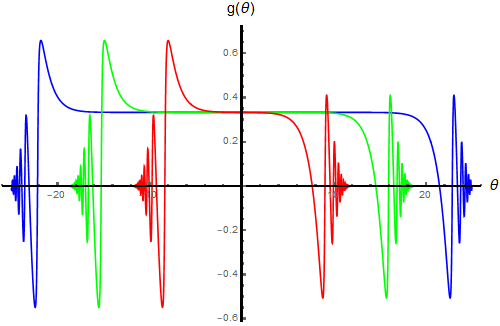
Figure 1: The formation of the plateau in $g(\theta)=-\frac{1}{2\pi}\mathcal{I}m\left(\ln\left(1+e^{-f_{\nu}(\theta+i0^{+})}\right)\right)$ as $m\rightarrow 0$ at $\beta^{2}=1/2$, $\alpha_{0}=1/6$. For this choice of the parameters, the height of the plateau of $g(\theta)$ is $1/3$.

Thus, perturbing the theory with the phase factor (246) with ${\bf{s}}=0$ is equivalent, in an appropriate scaling limit, to a constant shift of the volume $R$. At fixed normalisation of the deforming parameter $\tau$, the shift turns out to be directly proportional to the topological charge $Q_{0}$. We see, from (306) that the left- and right-mover sectors remain decoupled also at $\tau\neq 0$. However, starting directly from the CFT limit, one can argue that there exist less trivial ways to couple the two sectors. The most general variant involves four different coupling constants $\vec{\tau}=\{\tau^{(a|b)}\}$ with $a,b\in\{+,-\}$:

$$\mathcal{R}_{0}^{(\pm)}(\vec{\tau})=R\mp\left(\tau^{(\pm|+)}Q_{0}^{(+)}+\tau^{(\pm|-)}Q_{0}^{(-)}\right)\;,\quad Q_{0}^{(\pm)}=2\pi\alpha_{0}^{(\pm)}\beta^{2}\,.$$ (308)

Notice that in (308) we allowed the possibility for two different topological charges $Q^{(\pm)}_{0}$, associated to the $U(1)_{R}\times U(1)_{L}$ symmetry of the $c=1$ free (compactified) boson model, corresponding to the CFT limit of the sine-Gordon theory.

4.4 Further deformations involving the topological charge

A further, natural extension of the quantum models studied in section 4.2, corresponds to scattering phase factors of the form

$$\delta^{(\tilde{\bf{s}},{\bf{s}})}(\theta,\theta^{\prime})=\tau\,\gamma_{\tilde{\bf{s}}}\gamma_{{\bf{s}}}\sinh(\tilde{\bf{s}}\,\theta-{\bf{s}}\,\theta^{\prime})\;.$$ (309)

Deforming the kernel according to (247) and using (309) instead of (246), the driving term of (4.2) becomes

$$\nu=\nu(R,\alpha_{0}\,|\,\theta)-i\tau\tilde{\bf{s}}\,\gamma_{\tilde{s}}\Bigl{(}e^{\tilde{\bf{s}}\,\theta}I^{(\tilde{\bf{s}},{\bf{s}},-)}_{\bf{s}}-e^{-\tilde{\bf{s}}\,\theta}I^{(\tilde{\bf{s}},{\bf{s}},+)}_{\bf{s}}\Bigr{)}\;,$$ (310)

where $I_{{\bf{k}}}^{(\tilde{\bf{s}},{\bf{s}},\pm)}$ are defined through (267) and (268) with the deformed driving term (310). The cases with $\tilde{\bf{s}}=\pm 1$, have been extensively discussed in the previous sections, they all correspond to gravity-like theories, where the effect of the perturbation can be re-absorbed into a redefinition of the volume $R$ plus a shift in the rapidity $\theta$, according to (248). From equation (310), we see that for generic values of $\tilde{\bf{s}}\neq\pm 1$ it is not no longer possible to re-absorb the perturbation in the same fashion. However, another interesting example is recovered by considering the scaling limit $\{\tilde{\bf{s}},\gamma_{\tilde{\bf{s}}},m\}\rightarrow\{0,0,0\}$, such that $\tilde{\bf{s}}\,\gamma_{\tilde{\bf{s}}}$ remains finite. In the following we shall set $\tilde{\bf{s}}\,\gamma_{\tilde{\bf{s}}}=2\pi$. This situation corresponds to the standard massless limit where, in the undeformed $(\tau=0)$ NLIE, the right- $(+)$ and the left-mover $(-)$ sectors are completely decoupled, while a residual interaction between the two sectors is still present at $\tau\neq 0$. In fact, the deformed versions of $f_{\nu^{(\pm)}}(\theta)$ fulfil (4.3) with

$$\nu^{(\pm)}=\nu^{(\pm)}\bigl{(}R,\alpha_{0}^{(\pm)}-\alpha^{({\bf{s}},\pm)}\,|\,\theta\bigr{)}\;,\quad\alpha^{({\bf{s}},\pm)}=\Bigl{(}\tau^{(\pm)}I^{({\bf{s}},-)}_{\bf{s}}(R,\vec{\tau})-\tau^{(\mp)}I^{({\bf{s}},+)}_{\bf{s}}(R,\vec{\tau})\Bigr{)}\;,$$ (311)

where the charges $I^{({\bf{s}},\pm)}_{\bf{k}}$ are defined through (267) with driving term (311), and $\{\tau^{(-)},\tau^{(+)}\}=\vec{\tau}$ are two coupling parameters defined as

$$\tau^{(\pm)}=\tau e^{\pm\sigma}\,,\quad\pm\sigma=\lim_{\begin{subarray}{c}\theta\to\pm\infty\\ \tilde{\bf{s}}\to 0^{+}\end{subarray}}\tilde{\bf{s}}\,\theta\;.$$ (312)

Therefore, the contributions of the nontrivial interaction can be formally re-absorbed in a redefinition of the vacuum parameters $\alpha_{0}^{(\pm)}$. In turn, this affects the value of the effective central charges as

$$c^{({\bf{s}},\pm)}=c_{0}^{(\pm)}+24\beta^{2}(\alpha_{0}^{(\pm)})^{2}-24\beta^{2}\left((\alpha_{0}^{(\pm)})^{2}-\alpha^{({\bf{s}},\pm)}\right)^{2}\;,\quad c_{0}^{(\pm)}=c-24\beta^{2}(\alpha_{0}^{(\pm)})^{2}\;.$$ (313)

Considering the formal identification $Q_{0}^{(\pm)}=2\pi\alpha_{0}^{(\pm)}\beta^{2}$ made in (307), the redefinition (311) corresponds to the following dressing of the topological charges

$$Q^{({\bf{s}},\pm)}(R,\vec{\tau})=Q_{0}^{(\pm)}-\frac{\kappa}{4\pi}\Bigl{(}\tau^{(-)}I^{({\bf{s}},-)}_{\bf{s}}(R,\vec{\tau})-\tau^{(+)}I^{({\bf{s}},+)}_{\bf{s}}(R,\vec{\tau})\Bigr{)}\;,$$ (314)

with

$$\kappa=8\pi^{2}\beta^{2}\,.$$ (315)

Let us focus on the ${\bf{s}}=1$ case. The equations for the spectrum are

$$I^{(\pm)}_{1}(R,\vec{\tau})=\frac{2\pi}{R}\left(n^{(\pm)}-{\textstyle\frac{c^{(\pm)}}{24}}\right)\;,\quad(I^{(\pm)}_{1}=I^{(1,\pm)}_{1}\;,\;c^{(\pm)}=c^{(1,\pm)})\;,$$ (316)

which can be solved exactly for $I^{(\pm)}_{1}(R,\vec{\tau})$ at any values of the parameters $\tau^{(\pm)}$. However, since the general analytic expressions for $I^{(\pm)}_{1}$ are very cumbersome, we will restrict the discussion to specific scaling limits:

• $\tau^{(+)}=\tau^{(-)}=\tau$ :

  $$I^{(+)}_{1}(R,\tau)-I^{(-)}_{1}(R,\tau)=P(R)=\frac{2\pi}{R}\left(h^{(+)}-h^{(-)}\right)\;,$$ (317)

  $$I^{(+)}_{1}(R,\tau)=I_{1}^{(+)}(R)+\tau\frac{Q_{0}^{(\pm)}}{R}P(R)+\tau^{2}\frac{\kappa}{8\pi R}P^{2}(R)\;,$$ (318)

  with $h^{(\pm)}=h_{0}^{(\pm)}+n^{(\pm)}$ and (314) becomes

  $$Q^{(\pm)}(R,\tau)=Q_{0}^{(\pm)}+\tau\frac{\kappa}{4\pi}\,P(R)\;.$$ (319)

  Surprisingly, with the replacement

  $$I^{(\pm)}_{1}(R,\tau)=\frac{2\pi}{R}\left(h^{(\pm)}(\tau)-\frac{c}{24}\right)\;,$$ (320)

  equations (317) and (318) lead to exact expressions for the conformal dimensions $h^{(\pm)}(\tau)$, which precisely match the form of the (left) conformal dimension in the $\text{J}\bar{\text{T}}$ model, as recently shown in Guica:2019vnb :

  $$h^{(\pm)}(\tau)=h^{(\pm)}+\tau\frac{Q_{0}^{(\pm)}}{2\pi}P+\tau^{2}\frac{\kappa}{16\pi^{2}}P^{2}\,.$$ (321)

  As we will shortly see, this is the first instance among many that link the phase factor (309) with ${\bf{s}}=1$, in the scaling limit (312) to the quantum $\text{J}\bar{\text{T}}$ model.

• $\tau^{(+)}=0$ , $\tau^{(-)}=\tau$ : the two sectors $(\pm)$ are completely decoupled

  $$I^{(\pm)}_{1}(R,\tau) = I^{(\pm)}_{1}(R)\pm\tau\frac{Q_{0}^{(\pm)}}{R}I^{(\pm)}_{1}(R,\tau)+\tau^{2}\frac{\kappa}{8\pi R}\left(I^{(\pm)}_{1}(R,\tau)\right)^{2}\;,$$ (322)

  $$Q^{(\pm)}(R,\tau) = Q_{0}^{(\pm)}\pm\tau\frac{\kappa}{4\pi}\,I_{1}^{(\pm)}(R,\tau)\;,$$ (323)

  and the solutions to (322) are

  $$I^{(\pm)}_{1}(R,\tau)=\frac{4\pi}{\kappa\tau^{2}}\left(R\mp\tau Q_{0}^{(\pm)}-\sqrt{\left(R\mp\tau Q_{0}^{(\pm)}\right)^{2}-\tau^{2}\kappa\left(h^{(\pm)}-\frac{c}{24}\right)}\right)\;.$$ (324)

  We notice that (322) can be rewritten as

  $$I_{1}^{(\pm)}(R,\tau)=\frac{2\pi\left(h^{(\pm)}-\frac{c}{24}\right)}{R-\tau\left(\pm Q_{0}^{(\pm)}+\tau\frac{\kappa}{8\pi}I_{1}^{(\pm)}(R,\tau)\right)}\;,$$ (325)

  which suggests that, in this limit, the perturbation has a dual geometric description, since it can be interpreted as a redefinition of the length $R$. The dual deformation of the NLIE corresponds to a deformed version of $f_{\nu^{(\pm)}}(\theta)$ which fulfils (4.3) with

  $$\nu^{(\pm)}=\nu^{(\pm)}\left(\mathcal{R}^{(\pm)}_{0},\alpha_{0}\;\vline\;\theta\right)\;,\quad\mathcal{R}^{(\pm)}_{0}=R-\tau\left(\pm Q_{0}^{(\pm)}+\tau\frac{\kappa}{8\pi}I_{1}^{(\pm)}(R,\tau)\right)\;.$$ (326)

  Expressions (324) are trivially solutions of two decoupled Burgers-like equations

  $$\partial_{\tau}I_{1}^{(\pm)}(R,\tau)\pm Q^{(\pm)}(R,\tau)\,\partial_{R}I_{1}^{(\pm)}(R,\tau)=0\;.$$ (327)

  Therefore, $I_{1}^{(\pm)}(R,\tau)$ fulfils a Burgers-type equation analogous to (1), where $Q^{(\pm)}(R,\tau)$ play the role of velocities.

4.5 The quantum $\text{J}\bar{\text{T}}$ model

Formula (324) strongly resembles the expression for the energy of the right-movers of the $\text{J}\bar{\text{T}}$-deformed CFT derived in Bzowski:2018pcy ; Chakraborty:2018vja . To obtain the $\text{J}\bar{\text{T}}$ model, one must treat the $(\pm)$ sectors in a non-symmetric way. For ${\bf{s}}=1$, a possible asymmetric generalisation of (311) with four free parameters $\vec{\tau}=\{\tau^{(a|b)}\}$ with $a,b\in\{+,-\}$ is

$$\nu^{(\pm)}=\nu^{(\pm)}\bigl{(}R,\alpha_{0}^{(\pm)}-\alpha^{(\pm)}(\vec{\tau})\,|\,\theta\bigr{)}\;,$$

$$\alpha^{(\pm)}(\vec{\tau})=\Bigl{(}\tau^{(\pm|-)}I^{(-)}_{s}(R,\vec{\tau})-\tau^{(\mp|+)}I^{(+)}_{s}(R,\vec{\tau})\Bigr{)}\;.$$ (328)

In (328) we also included the possibility to have two different initial values of the twist parameters $\alpha_{0}^{(\pm)}$ in the two sectors. From (328), the $\text{J}\bar{\text{T}}$ model is recovered with the choice

$$\tau^{(\pm|-)}=0\;,\quad\tau^{(\mp|+)}=\tau\;,\quad\alpha_{0}^{(+)}=\alpha_{0}^{(-)}=\alpha_{0}\;.$$ (329)

Correspondingly, relations (328) become

$$\nu^{(\pm)}=\nu_{\text{J}\bar{\text{T}}}^{(\pm)}\left(R,\alpha_{0}-\alpha_{\text{J}\bar{\text{T}}}^{(\pm)}\;\vline\;\theta\right)\;,\quad\alpha_{\text{J}\bar{\text{T}}}^{(\pm)}=-\tau\,I_{\text{J}\bar{\text{T}}}^{(+)}(R,\tau)\;.$$ (330)

Alternatively, the $(+)$ sector can be equivalently described with a redefinition of the length $R$ as

$$\nu^{(+)}=\nu^{(+)}\left(\mathcal{R}_{\text{J}\bar{\text{T}}},\alpha_{0}\;\vline\;\theta\right)\;,\quad\mathcal{R}_{\text{J}\bar{\text{T}}}=R-\tau\left(Q_{0}+\tau\frac{\kappa}{8\pi}\,I_{\text{J}\bar{\text{T}}}^{(+)}(R,\tau)\right)\;.$$ (331)

The right-moving solution in (324) and the topological charge become

$$I^{(+)}_{1}(R,\tau)=I^{(+)}_{\text{J}\bar{\text{T}}}(R,\tau)=\frac{4\pi}{\kappa\tau^{2}}\left(R-\tau Q_{0}-\sqrt{\left(R-\tau Q_{0}\right)^{2}-\tau^{2}\kappa\left(h^{(+)}-\frac{c}{24}\right)}\right)\;,\quad$$ (332)

$$I_{\text{J}\bar{\text{T}}}^{(+)}(R,\tau)-I_{\text{J}\bar{\text{T}}}^{(-)}(R,\tau)=P(R)=\frac{2\pi}{R}\left(h^{(+)}-h^{(-)}\right)\;,$$ (333)

$$Q^{(+)}(R,\tau)=Q_{\text{J}\bar{\text{T}}}^{(+)}(R,\tau)=Q_{0}+\tau\,\frac{\kappa}{4\pi}\,I_{\text{J}\bar{\text{T}}}^{(+)}(R,\tau)\;.$$ (334)

Therefore, $Q_{0}=2\pi\alpha_{0}\beta^{2}$ and $\kappa=8\pi^{2}\beta^{2}$ have been again consistently identified with the topological charge and the chiral anomaly, respectively. The results described here are in full agreement with Bzowski:2018pcy and the classical results presented in section 3.

4.6 A simple example involving a pair of scattering phase factors

As already discussed, in principle one may introduce several scattering phase factors to deform the NLIEs. In this section we will consider a particular combination of ${\bf{s}}\to 0$ and $\tilde{\bf{s}}\to 0$ scattering factors which allows us to match with the classical results (208)–(209). We consider a double perturbation made of a length redefinition (308) with $\tau^{(\pm|+)}=\mp\tau$ and $\tau^{(\pm|-)}=\pm\tau$, together with a shift of the twist parameter (328) with $\tau^{(\mp|+)}=+\tau$ and $\tau^{(\pm|-)}=+\tau$. The corresponding deformed driving term is then

$$\nu^{(\pm)}=\nu^{(\pm)}\left(\mathcal{R}_{0}^{(\pm)},\alpha_{0}^{(\pm)}-\alpha^{(\pm)}(R,\tau)\;\vline\;\theta\right)\;,$$ (335)

with

$$\alpha^{(\pm)}(R,\tau)=-\tau\,P(R)\;,$$

$$\mathcal{R}_{0}^{(\pm)}=R+\tau\left(Q^{(+)}(R,\tau)-Q^{(-)}(R,\tau)\right)=R+\tau\left(Q_{0}^{(+)}-Q_{0}^{(-)}\right)\;,$$ (336)

where in the last equality we used the fact that $Q^{(\pm)}(R,\tau)=2\pi\,\beta^{2}\left(\alpha_{0}^{(\pm)}-\alpha^{(\pm)}(R,\tau)\right)$. Since the central charges are affected by the deformation as

$$c^{(\pm)}(R,\tau)=c+24\beta^{2}\bigl{(}\alpha_{0}^{(\pm)}\bigr{)}^{2}-24\beta^{2}\left(\alpha_{0}^{(\pm)}-\alpha^{(\pm)}(R,\tau)\right)^{2}\;,$$ (337)

one finds

$$I_{1}^{(\pm)}(R,\tau)=\frac{2\pi}{\mathcal{R}_{0}^{(\pm)}}\left(n^{(\pm)}-\frac{c^{(\pm)}(R,\tau)}{24}\right)=\frac{R\,I_{1}^{(\pm)}(R)+\tau\,Q_{0}^{(\pm)}P(R)+\frac{\kappa}{8\pi}\,\tau^{2}\,P^{2}(R)}{R+\tau\left(Q_{0}^{(+)}-Q_{0}^{(-)}\right)}\;,$$ (338)

$$I_{1}^{(+)}(R,\tau)-I_{1}^{(-)}(R,\tau)=P(R)\;,$$ (339)

$$Q^{(\pm)}(R,\tau)=Q_{0}^{(\pm)}+\tau\frac{\kappa}{4\pi}\,P(R)\;,$$ (340)

which match exactly with the results (208)–(209) obtained at the classical level for the corresponding densities.

5 Conclusions

In this paper, we have introduced and studied novel types of systems obtained by a local space-time deformation induced by higher-spin conserved charges. We have argued that these geometrical maps correspond to classical and quantum field theories perturbed by irrelevant Lorentz-breaking composite fields. The possibility of non-Lorentz invariant generalisations of the $\text{T}\bar{\text{T}}$ operator was first briefly discussed in Smirnov:2016lqw and the $\text{J}\bar{\text{T}}$ and the $\text{T}\bar{\text{J}}$ models studied in Guica:2017lia ; Bzowski:2018pcy ; Apolo:2018qpq ; Aharony:2018ics ; Chakraborty:2018vja ; Nakayama:2018ujt ; Araujo:2018rho are concrete realisations of these ideas, though with some important difference in the actual details. Another concise discussion on non-Lorentz invariant perturbations has appeared more recently in Cardy:2018jho were it was underlined the possibility to replace the $\text{T}\bar{\text{T}}$ operator with composite fields built out of a pair of conserved currents, a somehow obvious generalisation of the earlier comments Smirnov:2016lqw and results Guica:2017lia ; Bzowski:2018pcy ; Apolo:2018qpq ; Aharony:2018ics ; Chakraborty:2018vja ; Nakayama:2018ujt ; Araujo:2018rho which however also encompasses the systems effectively studied in the current paper. Here we would like to stress again that the spin $s$ in the scattering phase factor (247) can also assume non-integer values, therefore the extension to non-local conserved charges Bazhanov:1996dr appears to be straightforward, as also underlined in Smirnov:2016lqw .

Many open problems deserve further attention. First of all, the identification between the classical and the quantum results is, in our opinion, very convincing, but certainly more work is needed to fully confirm the match. In particular, a Lagrangian description for the higher-spin deformed models would lead the way to more stringent tests. Furthermore, it is natural to try to identify within the AdS₃/CFT₂ setup the corresponding (bulk) JJ and Yang-Baxter type deformations, as it was successfully done for their close relatives studied Guica:2017lia ; Bzowski:2018pcy ; Apolo:2018qpq ; Aharony:2018ics ; Chakraborty:2018vja ; Nakayama:2018ujt ; Araujo:2018rho . It would be important to extend the gravity setup adopted in Dubovsky:2017cnj ; Dubovsky:2018bmo to accommodate also these novel geometric deformations.

While the $\text{T}\bar{\text{T}}$ perturbation is compatible with supersymmetry Baggio:2018gct ; Dei:2018mfl ; Baggio:2018rpv ; Chang:2018dge ; Nakayama:2018ujt , higher spin Hamiltonians should, at least partially, lift the degeneracy of the states. Therefore, in general, supersymmetry should be explicitly broken by the more general perturbations discussed here. However, it would be interesting to find specific examples were a residual supersymmetry survives. Finally, it would be also nice to study the effect of these perturbations on 2D Yang-Mills Conti:2018jho ; Santilli:2018xux and, following the suggestion of Jiang:2019tcq , to study the expectation values on curved spacetimes, of the composite operators discussed here. Finally, while this paper was in its final writing stage the works Giveon:2019fgr ; LeFloch:2019rut appeared. The latter articles contain many interesting results on the $\text{J}\bar{\text{T}}$ model and the combined $\text{J}\bar{\text{T}}$/$\text{T}\bar{\text{T}}$ perturbations. There are only minor overlaps with the current paper. As already mentioned, our methods are easily generalisable to encompass such a two-coupling extension of the models described here, both at classical and quantum levels.

Acknowledgments – We are especially grateful to Riccardo Borsato, Patrick Dorey, Ferdinando Gliozzi, Yunfeng Jiang, Zohar Komargodski, Bruno Le Floch, Sergei Lukyanov, Marc Mezei, Domenico Orlando, Alessandro Sfondrini, Kentaroh Yoshida and Sasha Zamolodchikov for useful discussions. This project was partially supported by the INFN project SFT, the EU network GATIS+, NSF Award PHY-1620628, and by the FCT Project PTDC/MAT-PUR/30234/2017 “Irregular connections on algebraic curves and Quantum Field Theory". RT gratefully acknowledges support from the Simons Center for Geometry and Physics, Stony Brook University at which some of the research for this paper was performed.

Appendix A Deformed classical solutions

Following Conti:2018tca , we shall now describe how to derive explicitly a deformed solution $\phi^{({\bf{s}})}(\mathbf{z},\tau)$ associated to the change of variables (71) starting from the undeformed solution $\phi(\mathbf{w})$. First of all we compute the relation between the sets of coordinates $\mathbf{w}$ and $\mathbf{z}$ by integrating, for ${\bf{s}}\geq 0$, (81) for $\mathbf{z}$

$$\begin{cases}\frac{\partial z^{(s)}(\mathbf{w})}{\partial w}=1+2\tau\,\bar{\Theta}_{s-1}(\mathbf{w})\,,\\ \frac{\partial z^{(s)}(\mathbf{w})}{\partial\bar{w}}=2\tau\,\bar{\rm T}_{s+1}(\mathbf{w})\,,\end{cases}\;\quad\begin{cases}\frac{\partial\bar{z}^{(s)}(\mathbf{w})}{\partial w}=2\tau\,{\rm T}_{s+1}(\mathbf{w})\,,\\ \frac{\partial\bar{z}^{(s)}(\mathbf{w})}{\partial\bar{w}}=1+2\tau\,\Theta_{s-1}(\mathbf{w})\,,\end{cases}$$ (341)

where we have denoted $\mathbf{z}=\mathbf{z}^{(s)}$ to distinguish between the different perturbations. The components of the higher charges ${\rm T}_{s+1}(\mathbf{w})$, $\Theta_{s-1}(\mathbf{w})$ along with their complex conjugates are implicitly evaluated on the specific field configuration $\phi(\mathbf{w})$. Inverting the relation $\mathbf{z}^{(s)}(\mathbf{w})$, we find the deformed solution as

$$\phi^{(s)}\bigl{(}\mathbf{z},\tau\bigr{)}=\phi\Bigl{(}\mathbf{w}\bigl{(}\mathbf{z}^{(s)}\bigr{)}\Bigr{)}\;.$$ (342)

Similarly, we can apply the same strategy to derive a deformed solution associated to the change of variables (76), for ${\bf{s}}\leq 0$. In this case we should, instead, integrate the system

$$\begin{cases}\frac{\partial z^{(s^{\prime})}(\mathbf{w})}{\partial w}=1+2\tau\,{\rm T}_{s+1}(\mathbf{w})\,,\\ \frac{\partial z^{(s^{\prime})}(\mathbf{w})}{\partial\bar{w}}=2\tau\,\Theta_{s-1}(\mathbf{w})\,,\end{cases}\;\quad\begin{cases}\frac{\partial\bar{z}^{(s^{\prime})}(\mathbf{w})}{\partial w}=2\tau\,\bar{\Theta}_{s-1}(\mathbf{w})\,,\\ \frac{\partial\bar{z}^{(s^{\prime})}(\mathbf{w})}{\partial\bar{w}}=1+2\tau\,\bar{\rm T}_{s+1}(\mathbf{w})\,,\end{cases}\;$$ (343)

and repeat the same procedure described above.

A.1 Explicit Lorentz breaking in a simple example

The purpose of this section is to highlight the difference between the $\text{T}\bar{\text{T}}$ perturbation and those corresponding to spins ${\bf{s}}\neq 1$, through the study of a simple example. Since perturbations with higher spins should break explicitly Lorentz symmetry, it is convenient to start from a solution of the Laplace equation which is particularly symmetric under rotations i.e. the “spiral staircase" solution of Gutshabash:2017qxl :

$$\phi(\mathbf{w})=d\,\ln{\left(\frac{w+\xi}{\bar{w}+\bar{\xi}}\right)}\;,\quad(\xi,\bar{\xi}\in\mathbb{C}\;,\quad d\in\mathbb{R})\;,$$ (344)

where $w$ and $\bar{w}$ are complex conjugated variables related to the cartesian coordinates $\mathbf{y}=(y^{1},y^{2})$ through (12). Using

$$\partial_{\bar{w}}\frac{1}{w+\xi}=-\pi\,\delta(w+\xi)\;,\quad\partial_{w}\frac{1}{\bar{w}+\bar{\xi}}=-\pi\,\delta(\bar{w}+\bar{\xi})\;,$$ (345)

one can show that (344) is indeed solution to the undeformed EoMs: $\partial_{w}\partial_{\bar{w}}\phi=0$.
For sake of brevity, we will only consider perturbations induced by the set of charges (51), the deformations associated to (50) can be obtained from the results described here through a simple redefinition of the coupling $\tau$.
Integrating (341) using the set of charges (51) evaluated on the solution (344) we obtain

$$z^{(s)}(\mathbf{w})=w+\tau\,\frac{\Gamma\bigl{(}\frac{s+1}{2}\bigr{)}^{2}}{s}\frac{d^{2}}{(\bar{w}+\bar{\xi})^{s}}\;,\quad\bar{z}^{(s)}(\mathbf{w})=\bar{w}+\tau\,\frac{\Gamma\bigl{(}\frac{s+1}{2}\bigr{)}^{2}}{s}\frac{d^{2}}{(w+\xi)^{s}}\;.$$ (346)

The latter equations cannot explicitly be inverted, for generic spin $s$, as $\mathbf{w}\left(\mathbf{z}^{(s)}\right)$. However, for $s=1$, i.e. the $\text{T}\bar{\text{T}}$ perturbation, (346) can be written as

$$z+\xi=(w+\xi)\Biggl{[}1+\tau\frac{d^{2}}{(w+\xi)(\bar{w}+\bar{\xi})}\Biggr{]}\;,\quad\bar{z}+\bar{\xi} = (\bar{w}+\bar{\xi})\Biggl{[}1+\tau\frac{d^{2}}{(w+\xi)(\bar{w}+\bar{\xi})}\Biggr{]}\;,$$ (347)

with $\mathbf{z}=\mathbf{z}^{(1)}(\mathbf{w})$, from which

$$\phi(\mathbf{w})=d\,\ln{\left(\frac{w+\xi}{\bar{w}+\bar{\xi}}\right)}=d\,\ln{\left(\frac{z+\xi}{\bar{z}+\bar{\xi}}\right)}=\phi(\mathbf{z},\tau)\;.$$ (348)

Therefore, the solution (344) is a fixed point of the $\text{T}\bar{\text{T}}$ flow. To clearly see how the ${\bf{s}}\neq 1$ perturbations affect the solution (344), we shall restrict to the ${\bf{s}}<0$ perturbations, where the deformed solutions can be found explicitly. Integrating (343) using the set of charges (51), again evaluated on (344), we find

$$z^{(s^{\prime})}(\mathbf{w})=w+\tau\,\frac{\Gamma\bigl{(}\frac{s+1}{2}\bigr{)}^{2}}{s}\frac{d^{2}}{(w+\xi)^{s}}\;,\quad\bar{z}^{(s^{\prime})}(\mathbf{w})=\bar{w}+\tau\,\frac{\Gamma\bigl{(}\frac{s+1}{2}\bigr{)}^{2}}{s}\frac{d^{2}}{(\bar{w}+\bar{\xi})^{s}}\;.$$ (349)

Comparing (346) with (349) we see that the difference between the ${\bf{s}}>0$ and ${\bf{s}}<0$ perturbations lies in the substitution $w+\xi\longleftrightarrow\bar{w}+\bar{\xi}$ in the term proportional to $\tau$, which implies that, for ${\bf{s}}<0$, there is no mixing between holomorphic and anti-holomorphic components.
Since holomorphic and anti-holomorphic parts are completely decoupled, we can integrate explicitly (349) for $w$ and $\bar{w}$. The result is

$$w\bigl{(}\mathbf{z}^{(s^{\prime})}\bigr{)} = z^{(s^{\prime})}+\frac{s}{1+s}\left[-1+F_{s}\left(\left(\frac{1+s}{s}\right)^{1+s}\Gamma\biggl{(}\frac{1+s}{2}\biggr{)}^{2}\frac{\tau\,d^{2}}{\bigl{(}z^{(s^{\prime})}+\xi\bigr{)}^{1+s}}\right)\right]\bigl{(}z^{(s^{\prime})}+\xi\bigr{)}\;,$$

$$\bar{w}\bigl{(}\mathbf{z}^{(s^{\prime})}\bigr{)} = \bar{z}^{(s^{\prime})}+\frac{s}{1+s}\left[-1+F_{s}\left(\left(\frac{1+s}{s}\right)^{1+s}\Gamma\biggl{(}\frac{1+s}{2}\biggr{)}^{2}\frac{\tau\,d^{2}}{\bigl{(}\bar{z}^{(s^{\prime})}+\bar{\xi}\bigr{)}^{1+s}}\right)\right]\bigl{(}\bar{z}^{(s^{\prime})}+\bar{\xi}\bigr{)}\;,$$

Finally, the deformed solutions are recovered by plugging (A.1) into (344)

$$\phi^{(s^{\prime})}(\mathbf{z},\tau)=d\,\ln{\left(\frac{z+\xi}{\bar{z}+\bar{\xi}}\right)}+d\,\ln{\left(\frac{1+s\,F_{s}\left(\left(\frac{1+s}{s}\right)^{1+s}\Gamma\bigl{(}\frac{1+s}{2}\bigr{)}^{2}\frac{\tau\,d^{2}}{(z+\xi)^{1+s}}\right)}{1+s\,F_{s}\left(\left(\frac{1+s}{s}\right)^{1+s}\Gamma\bigl{(}\frac{1+s}{2}\bigr{)}^{2}\frac{\tau\,d^{2}}{(\bar{z}+\bar{\xi})^{1+s}}\right)}\right)}\;.$$ (351)

Let us discuss in detail the case ${\bf{s}}=-1$ of (351),

$$\phi^{(-1)}(\mathbf{z},\tau)=d\,\ln{\left(\frac{z+\xi}{\bar{z}+\bar{\xi}}\right)}+d\,\ln{\left(\frac{1+\sqrt{1-\frac{4\tau\,d^{2}}{(z+\xi)^{2}}}}{1+\sqrt{1-\frac{4\tau\,d^{2}}{(\bar{z}+\bar{\xi})^{2}}}}\right)}\;.$$ (352)

We observe that, as soon as the perturbation is switched on, a pair of square root branch points appears at $z=\pm 2d\sqrt{\tau}-\xi$. Considering for simplicity $\xi,\bar{\xi}\in\mathbb{R}$, they form a branch cut on the real axis of the complex plane of $z$

$$\mathcal{C}=\left(-2d\sqrt{\tau}-\xi;+2d\sqrt{\tau}-\xi\right)\;,$$ (353)

i.e. the black line in Figure 2b.

(a) ${\bf{s}}=1$

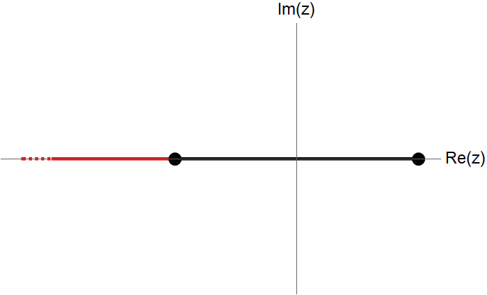
(b) ${\bf{s}}=-1$

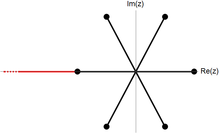
(c) ${\bf{s}}=-3$

Figure 2: Analytic structure of the deformed solution (351) in the complex plane of $z$ for different values of ${\bf{s}}$, with $\xi=\bar{\xi}=0$. The black lines correspond to the square root branch cuts connecting the singularities (358), while the red lines correspond to the logarithmic cuts.

Instead, the logarithmic singularity of the undeformed solution (344) at $w=-\xi$ cancels out with the singularities coming from the additional term in (352). Therefore, the logarithmic cut of (344) which runs, in our convention, along the real axis from $w=-\infty$ to $w=-\xi$, now connects $z=-\infty$ on the first sheet to $z=-\infty$ on the secondary branches reached by passing through $\mathcal{C}$ (see the red line in Figure 2b). This implies that the behaviour of (352) at $z=\infty$ is different according to the choice of the branch. On the first sheet one has

$$\phi^{(-1)}(\mathbf{z},\tau)\underset{\underset{(1\text{-th sheet})}{\mathbf{z}\to\infty}}{\sim}d\,\ln{\left(\frac{z+\xi}{\bar{z}+\bar{\xi}}\right)}+\mathcal{O}(z^{0})\;,$$ (354)

while, on the second sheet, flipping the $+$ sign in front of the square roots in (352) into a $-$ sign one finds

$$\phi^{(-1)}(\mathbf{z},\tau)\underset{\underset{(2\text{-nd sheet})}{\mathbf{z}\to\infty}}{\sim}-d\,\ln{\left(\frac{z+\xi}{\bar{z}+\bar{\xi}}\right)}+\mathcal{O}(z^{0})\;.$$ (355)

In Figure 3, is represented the Riemann surface of the solution (352) (Figure 3b) together with that of the bare solution (Figure 3a), which coincides with the $\text{T}\bar{\text{T}}$ deformed solution. Notice that the analytic structure of (352) can be read out from the implicit map (349). In fact, for ${\bf{s}}=-1$, equation (349) reduces to the Zhukovsky transformation

$$z+\xi=(w+\xi)+\tau\,\frac{d}{(w+\xi)}\;,\quad\bar{z}+\bar{\xi}=(\bar{w}+\bar{\xi})+\tau\,\frac{d}{(\bar{w}+\bar{\xi})}\;,$$ (356)

from which we see that $z=\infty$ on the first sheet is mapped into $w=\infty$, while $z=\infty$ on the second sheet is mapped into $w=-\xi$. Moreover (356) captures the large $z$ behaviour of the solution. In fact,

$$d\,\ln{\left(\frac{w+\xi}{\bar{w}+\bar{\xi}}\right)}\underset{w\to\infty}{\sim}d\,\ln{\left(\frac{z+\xi}{\bar{z}+\bar{\xi}}\right)}\;,\quad d\,\ln{\left(\frac{w+\xi}{\bar{w}+\bar{\xi}}\right)}\underset{w\to-\xi}{\sim}-d\,\ln{\left(\frac{z+\xi}{\bar{z}+\bar{\xi}}\right)}\;.$$ (357)

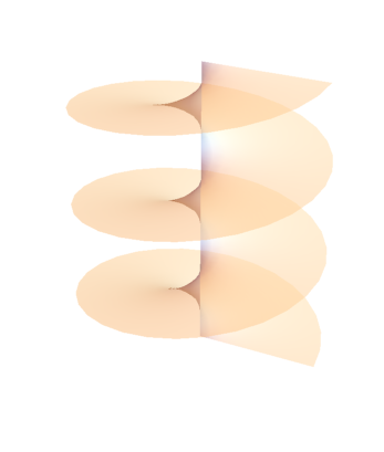
(a)

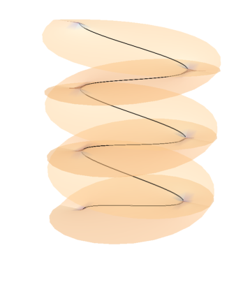
(b)

Figure 3: Riemann surface of the deformed solution $\phi^{({\bf{s}})}(\mathbf{z},\tau)$ , $(\xi=\bar{\xi}=0)$, in the complex plane of $z$ for ${\bf{s}}=1$ (a), and ${\bf{s}}=-1$ (b).

Let us now consider the generic solution (351). The hypergeometric functions appearing in (351) are of the form $\,{}_{p+1}F_{p}(a_{1},\dots,a_{p+1};b_{1},\dots,b_{p};x)$, with coefficients $\{a_{i}\}_{i=1}^{p+1},\;\{b_{j}\}_{j=1}^{p}\in\mathbb{Q}$. Generally, these hypergeometric functions have branch points at $x=\infty$ and $x=1$, which in our case are mapped into $z=0$ and

$$x_{n}=\frac{1+s}{s}\left(d\,\Gamma\left(\frac{1+s}{2}\right)\right)^{\frac{2}{1+s}}\tau^{\frac{1}{1+s}}e^{\frac{2\pi i}{1+s}n}-\xi\;,\quad(n=0,\dots,s)\;,$$ (358)

respectively. The branch points (358) are all of square root type. In conclusion, roughly speaking, starting from a rotational-symmetric solution, the perturbations with ${\bf{s}}<0$ have explicitly broken the original $U(1)$ symmetry down to a discrete $Z_{2s}$.

Appendix B Burgers equations

We want to prove that the general Burgers equations (256), which we report here for convenience

$$\partial_{\tau}I_{{\bf{k}}}^{({\bf{s}},\pm)}(R,\tau)+R^{\prime}\partial_{R}I_{{\bf{k}}}^{({\bf{s}},\pm)}(R,\tau)=\pm{\bf{k}}\,\theta^{\prime}_{0}I_{{\bf{k}}}^{({\bf{s}},\pm)}(R,\tau)\;,$$ (359)

with $R^{\prime}$ and $\theta_{0}^{\prime}$ defined through (4.2), reduce to

$$\partial_{\tau}I_{k}^{(s,\pm)}(R,\tau) = 2I_{s}^{(s,\mp)}(R,\tau)\,\partial_{R}I_{k}^{(s,\pm)}(R,\tau)\;,\quad(\mathbf{s}=s>0)\;,$$ (360)

$$\partial_{\tau}I_{k^{\prime}}^{(s^{\prime},\pm)}(R,\tau) = 2I_{s^{\prime}}^{(s^{\prime},\pm)}(R,\tau)\,\partial_{R}I_{k^{\prime}}^{(s^{\prime},\pm)}(R,\tau)\;,\quad(\mathbf{s}=s^{\prime}=-s<0)\;,$$ (361)

in the CFT limit.
Let us begin with the $\mathbf{s}<0$ case. From the implicit relation (284)

$$I_{k^{\prime}}^{(s^{\prime},\pm)}(R,\tau)=I_{k^{\prime}}^{(s^{\prime},\pm)}\left(\mathcal{R}_{0}^{(s^{\prime},\mp)}\right)\;,$$ (362)

using (281), we have

$$I_{k^{\prime}}^{(s^{\prime},\pm)}(R,\tau)=\frac{2\pi a_{k^{\prime}}}{\left(R+2\tau I_{s^{\prime}}^{(s^{\prime},\pm)}(R,\tau)\right)^{k}}\;.$$ (363)

Differentiating (363) w.r.t. $R$ for $k^{\prime}=s^{\prime}$ $(k=s)$, we first express $I_{s^{\prime}}^{(s^{\prime},\pm)}(R,\tau)$ as a function of $\partial_{R}I_{s^{\prime}}^{(s^{\prime},\pm)}(R,\tau)$ as

$$I_{s^{\prime}}^{(s^{\prime},\pm)}(R,\tau)=-\frac{R\,\partial_{R}I_{s^{\prime}}^{(s^{\prime},\pm)}(R,\tau)}{2\tau s(1+s)\,\partial_{R}I_{s^{\prime}}^{(s^{\prime},\pm)}(R,\tau)}\;.$$ (364)

Then, differentiating again (363) w.r.t. $R$ for generic $k^{\prime}$ $(k)$ and using (364), we express $I_{k^{\prime}}^{(s^{\prime},\pm)}(R,\tau)$ as a function of $\partial_{R}I_{s^{\prime}}^{(s^{\prime},\pm)}(R,\tau)$ and $\partial_{R}I_{k^{\prime}}^{(s^{\prime},\pm)}(R,\tau)$ as follows

$$I_{k^{\prime}}^{(s^{\prime},\pm)}(R,\tau)=-\frac{s}{k}\frac{R\,\partial_{R}I_{k^{\prime}}^{(s^{\prime},\pm)}(R,\tau)}{2\tau s(1+s)\,\partial_{R}I_{s^{\prime}}^{(s^{\prime},\pm)}(R,\tau)}\;.$$ (365)

Finally, using (365), it is a matter of simple algebraic manipulation to show that

$$-R^{\prime}\partial_{R}I_{k^{\prime}}^{(s^{\prime},\pm)}(R,\tau)+k^{\prime}\theta_{0}^{\prime}I_{k^{\prime}}^{(s^{\prime},\pm)}(R,\tau)=2I_{s^{\prime}}^{(s^{\prime},\pm)}(R,\tau)\,\partial_{R}I_{k^{\prime}}^{(s^{\prime},\pm)}(R,\tau)\;,$$ (366)

which proves that (256) for ${\bf{k}}=k^{\prime}$ and ${\bf{s}}=s^{\prime}$ reduce to (361).
Considering the $\mathbf{s}>0$ case, from the implicit relation (283)

$$I_{k}^{(s,\pm)}(R,\tau)=I_{k}^{(s,\pm)}\left(\mathcal{R}_{0}^{(s,\pm)}\right)\;,$$ (367)

using (281), we have

$$I_{k}^{(s,\pm)}(R,\tau)=\frac{2\pi a_{k}}{\left(R+2\tau I_{s}^{(s,\mp)}(R,\tau)\right)^{k}}\;.$$ (368)

Repeating the same procedure as in the ${\bf{s}}<0$ case, we express $I_{k}^{(s,\pm)}(R,\tau)$ as a function of $\partial_{R}I_{k}^{(s,\pm)}$ and $\partial_{R}I_{s}^{(s,\pm)}$ as follows

$$I_{k}^{(s,\pm)}=-\frac{s}{k}\frac{R\,\partial_{R}I_{k}^{(s,\pm)}\left(2\tau s\,\partial_{R}I_{s}^{(s,\pm)}-2\tau\partial_{R}I_{k}^{(s,\mp)}+s\right)}{s^{2}\left(1+2\tau\,\partial_{R}I_{s}^{(s,+)}+2\tau\,\partial_{R}I_{s}^{(s,-)}\right)+4\left(s^{2}-1\right)\tau^{2}\,\partial_{R}I_{s}^{(s,+)}\,\partial_{R}I_{s}^{(s,-)}}\;,$$ (369)

Again, using (369), one can show that the following relation holds

$$-R^{\prime}\partial_{R}I_{k}^{(s,\pm)}+k\theta_{0}^{\prime}I_{k}^{(s,\pm)}=2I_{s}^{(s,\mp)}\,\partial_{R}I_{k}^{(s,\pm)}\;,$$ (370)

which proves that (256) for ${\bf{k}}=k$ and ${\bf{s}}=s$ reduce to (360).

References

- (1) F. A. Smirnov and A. B. Zamolodchikov, On space of integrable quantum field theories, Nucl. Phys. B915 (2017) 363–383 [arXiv:1608.05499].
- (2) A. Cavaglià, S. Negro, I. M. Szécésnyi and R. Tateo, -deformed 2D Quantum Field Theories, JHEP 10 (2016) 112 [arXiv:1608.05534].
- (3) A. B. Zamolodchikov, Expectation value of composite field in two-dimensional quantum field theory, hep-th/0401146.
- (4) S. Dubovsky, R. Flauger and V. Gorbenko, Solving the Simplest Theory of Quantum Gravity, JHEP 09 (2012) 133 [arXiv:1205.6805].
- (5) S. Dubovsky, R. Flauger and V. Gorbenko, Effective String Theory Revisited, JHEP 09 (2012) 044 [arXiv:1203.1054].
- (6) M. Caselle, D. Fioravanti, F. Gliozzi and R. Tateo, Quantisation of the effective string with TBA, JHEP 07 (2013) 071 [arXiv:1305.1278].
- (7) C. Chen, P. Conkey, S. Dubovsky and G. Hernandez-Chifflet, Undressing Confining Flux Tubes with , Phys. Rev. D98 (2018), no. 11 114024 [arXiv:1808.01339].
- (8) L. McGough, M. Mezei and H. Verlinde, Moving the CFT into the bulk with , JHEP 04 (2018) 010 [arXiv:1611.03470].
- (9) G. Turiaci and H. Verlinde, Towards a 2d QFT Analog of the SYK Model, JHEP 10 (2017) 167 [arXiv:1701.00528].
- (10) A. Giveon, N. Itzhaki and D. Kutasov, and LST, JHEP 07 (2017) 122 [arXiv:1701.05576].
- (11) A. Giveon, N. Itzhaki and D. Kutasov, A solvable irrelevant deformation of AdS3/CFT2, JHEP 12 (2017) 155 [arXiv:1707.05800].
- (12) M. Asrat, A. Giveon, N. Itzhaki and D. Kutasov, Holography Beyond AdS, Nucl. Phys. B932 (2018) 241–253 [arXiv:1711.02690].
- (13) G. Giribet, -deformations, AdS/CFT and correlation functions, JHEP 02 (2018) 114 [arXiv:1711.02716].
- (14) P. Kraus, J. Liu and D. Marolf, Cutoff AdS3 versus the deformation, JHEP 07 (2018) 027 [arXiv:1801.02714].
- (15) W. Cottrell and A. Hashimoto, Comments on double trace deformations and boundary conditions, Phys. Lett. B789 (2019) 251–255 [arXiv:1801.09708].
- (16) M. Baggio and A. Sfondrini, Strings on NS-NS Backgrounds as Integrable Deformations, Phys. Rev. D98 (2018), no. 2 021902 [arXiv:1804.01998].
- (17) J. P. Babaro, V. F. Foit, G. Giribet and M. Leoni, type deformation in the presence of a boundary, JHEP 08 (2018) 096 [arXiv:1806.10713].
- (18) R. Conti, S. Negro and R. Tateo, The perturbation and its geometric interpretation, JHEP 02 (2019) 085 [arXiv:1809.09593].
- (19) S. Dubovsky, V. Gorbenko and M. Mirbabayi, Asymptotic fragility, near AdS2 holography and , JHEP 09 (2017) 136 [arXiv:1706.06604].
- (20) G. Bonelli, N. Doroud and M. Zhu, -deformations in closed form, JHEP 06 (2018) 149 [arXiv:1804.10967].
- (21) R. Conti, L. Iannella, S. Negro and R. Tateo, Generalised Born-Infeld models, Lax operators and the perturbation, JHEP 11 (2018) 007 [arXiv:1806.11515].
- (22) M. Guica, An integrable Lorentz-breaking deformation of two-dimensional CFTs, SciPost Phys. 5 (2018), no. 5 048 [arXiv:1710.08415].
- (23) A. Bzowski and M. Guica, The holographic interpretation of -deformed CFTs, JHEP 01 (2019) 198 [arXiv:1803.09753].
- (24) L. Apolo and W. Song, Strings on warped AdS3 via deformations, JHEP 10 (2018) 165 [arXiv:1806.10127].
- (25) O. Aharony, S. Datta, A. Giveon, Y. Jiang and D. Kutasov, Modular covariance and uniqueness of deformed CFTs, JHEP 01 (2019) 085 [arXiv:1808.08978].
- (26) S. Chakraborty, A. Giveon and D. Kutasov, deformed CFT2 and string theory, JHEP 10 (2018) 057 [arXiv:1806.09667].
- (27) Y. Nakayama, Very Special deformed CFT, arXiv:1811.02173.
- (28) T. Araujo, E. Colgain, Y. Sakatani, M. M. Sheikh-Jabbari and H. Yavartanoo, Holographic integration of and via , JHEP 03 (2019) 168 [arXiv:1811.03050].
- (29) B. Le Floch and M. Mezei, KdV charges in theories and new models with super-Hagedorn behavior, arXiv:1907.02516.
- (30) Al. B. Zamolodchikov, From tricritical Ising to critical Ising by thermodynamic Bethe ansatz, Nucl. Phys. B358 (1991) 524–546.
- (31) R. Conti, S. Negro and R. Tateo, In preparation, .
- (32) B. Le Floch and M. Mezei, Solving a family of -like theories, arXiv:1903.07606.
- (33) G. Arutyunov and S. Frolov, On String S-matrix, Bound States and TBA, JHEP 12 (2007) 024 [arXiv:0710.1568].
- (34) A. Klümper and P. Pearce, Conformal weights of RSOS lattice models and their fusion hierarchies, Physica A 183 (1992) 304.
- (35) P. Pearce and A. Klümper, Finite-size corrections and scaling dimensions of solvable lattice models: An analytic method, Phys. Rev. Lett. 66 (1991) 974–977.
- (36) C. Destri and H. de Vega, New thermodynamic Bethe Ansatz equations without strings, Phys. Rev. Lett. 69 (Oct, 1992) 2313–2317.
- (37) D. Fioravanti, A. Mariottini, E. Quattrini and F. Ravanini, Excited state Destri-De Vega equation for Sine-Gordon and restricted Sine-Gordon models, Phys. Lett. B 390 (1997) 243–251 [hep-th/9608091].
- (38) G. Feverati, F. Ravanini and G. Takacs, Nonlinear integral equation and finite volume spectrum of Sine-Gordon theory, Nucl. Phys. B540 (1999) 543–586 [hep-th/9805117].
- (39) V. V. Bazhanov, S. L. Lukyanov and A. B. Zamolodchikov, Integrable structure of conformal field theory, quantum KdV theory and thermodynamic Bethe ansatz, Commun. Math. Phys. 177 (1996) 381–398 [hep-th/9412229].
- (40) V. V. Bazhanov, S. L. Lukyanov and A. B. Zamolodchikov, Integrable quantum field theories in finite volume: Excited state energies, Nucl. Phys. B489 (1997) 487–531 [hep-th/9607099].
- (41) G. Feverati, F. Ravanini and G. Takacs, Nonlinear integral equation and finite volume spectrum of minimal models perturbed by Phi(1,3), Nucl. Phys. B570 (2000) 615–643 [hep-th/9909031].
- (42) P. Dorey and R. Tateo, Excited states by analytic continuation of TBA equations, Nucl. Phys. B 482 (1996) 639–659 [hep-th/9607167].
- (43) S. L. Lukyanov and A. B. Zamolodchikov, Quantum Sine(h)-Gordon Model and Classical Integrable Equations, JHEP 07 (2010) 008 [arXiv:1003.5333].
- (44) A. Cavaglià, D. Fioravanti and R. Tateo, Extended Y-system for the correspondence, Nucl. Phys. B843 (2011) 302–343 [arXiv:1005.3016].
- (45) Y. Jiang, Lectures on solvable irrelevant deformations of 2d quantum field theory, arXiv:1904.13376.
- (46) V. V. Bazhanov, S. L. Lukyanov and A. B. Zamolodchikov, Integrable structure of conformal field theory. 2. Q operator and DDV equation, Commun. Math. Phys. 190 (1997) 247–278 [hep-th/9604044].
- (47) S. L. Lukyanov, Low energy effective Hamiltonian for the XXZ spin chain, Nucl. Phys. B522 (1998) 533–549 [cond-mat/9712314].
- (48) D. Bernard and A. Leclair, Quantum group symmetries and nonlocal currents in 2-D QFT, Commun. Math. Phys. 142 (1991) 99–138.
- (49) A. Zamolodchikov, Thermodynamic Bethe Ansatz in Relativistic Models. Scaling Three State Potts and Lee-Yang Models, Nucl. Phys. B 342 (1990) 695–720.
- (50) M. Guica, On correlation functions in -deformed CFTs, arXiv:1902.01434.
- (51) J. Cardy, deformations of non-Lorentz invariant field theories, arXiv:1809.07849.
- (52) S. Dubovsky, V. Gorbenko and G. Hernandez-Chifflet, partition function from topological gravity, JHEP 09 (2018) 158 [arXiv:1805.07386].
- (53) A. Dei and A. Sfondrini, Integrable spin chain for stringy Wess-Zumino-Witten models, JHEP 07 (2018) 109 [arXiv:1806.00422].
- (54) M. Baggio, A. Sfondrini, G. Tartaglino-Mazzucchelli and H. Walsh, On deformations and supersymmetry, arXiv:1811.00533.
- (55) C.-K. Chang, C. Ferko and S. Sethi, Supersymmetry and Deformations, arXiv:1811.01895.
- (56) L. Santilli and M. Tierz, Large N phase transition in -deformed 2d Yang-Mills theory on the sphere, JHEP 01 (2019) 054 [arXiv:1810.05404].
- (57) Y. Jiang, Expectation value of operator in curved spacetimes, arXiv:1903.07561.
- (58) A. Giveon, Comments on , and String Theory, arXiv:1903.06883.
- (59) E. S. Gutshabash and P. P. Kulish, New exact solutions of the Born-Infeld model, Zap. Nauchn. Semin. 465 (2017) 135–146.