Random Fragments Classification of Microbial Marker Clades with Multi-class SVM and N-Best Algorithm

Abstract

Microbial clades modeling is a challenging problem in biology based on microarray genome sequences, especially in new species gene isolates discovery and category. Marker family genome sequences play important roles in describing specific microbial clades within species, a framework of support vector machine (SVM) based microbial species classification with N-best algorithm is constructed to classify the centroid marker genome fragments randomly generated from marker genome sequences on MetaRef. A time series feature extraction method is proposed by segmenting the centroid gene sequences and mapping into different dimensional spaces. Two ways of data splitting are investigated according to random splitting fragments along genome sequence (DI) , or separating genome sequences into two parts (DII).Two strategies of fragments recognition tasks, dimension-by-dimension and sequence–by–sequence, are investigated. The k-mer size selection, overlap of segmentation and effects of random split percents are also discussed. Experiments on 12390 maker genome sequences belonging to marker families of 17 species from MetaRef show that, both for DI and DII in dimension-by-dimension and sequence-by-sequence recognition, the recognition accuracy rates can achieve above 28% in top-1 candidate, and above 91% in top-10 candidate both on training and testing sets overall.

1 Introduction

Tremendous genomic sequences measured by new generation sequencing machines from second-generation (2G) to third-generation (3G) and fourth-generation (4G) platforms [1] put forward high level requirement of automatical classification and identification for genomic analysis techniques. Designing more accurate and effective models for clades or species classification and disease diagnose are challenging problems facing the sea amount of genomic fragments. In recent three decades, many machine learning and statistical learning methods are developed in genomic analysis, such as BLAST[2-4], hidden Markov model (HMM) [5-15], support vector machine (SVM)[16-34], combination of linear discriminant analysis (LDA) and artificial neural network (ANN) [35], etc.

HMM is a powerful model in microbial clade classification and genome associate disease analysis [5,14,15]. However, HMM has a limitation in genomic analysis that the number of states in HMM model ($4^{k}$) grows exponentially with the increasing of k-mer size, and consequently leading to spareness of gene segments for training each state, this phenomenon is distinct especially in rare microbes and diseases. SVM is another popular technique to solve the relative sparse data case in pattern recognition and machine learning [36-39]. Many SVM literatures address the prediction of the microbial genomes classification and prediction [16,23,28,31]. The standard SVM [36-39] is adopted in our fragments modeling.

Feature selection is the first and key step in genomic information analysis. k-mer based sequence binning method and K-means clustering method are two widely used techniques in genomic analysis. k-mer binning method is widely adopted in genomic analysis[40-43], SVM–based genomic analysis[31], and LDA & ANN based genomic analysis platform[35]. K–means clustering is utilized in both HMM–based [7] and SVM–based genomic analysis[28]. Although these two preprocessing methods can obtain statistical property of genome sequences, they may mask and neglect the subtle or particular local information along genome sequence. In genomic analysis, the genomic information in some species or diseases DNA sequences may exist in some local position under some kinds of measurements. The difference among various cancers DNA sequences from a same human being may appear in some local places of human DNA sequences under an appropriate measurement. For microbial classification, the ideal model of classification and clustering is to make the fragments in same specie more closer than those from other species. Hence, the real fragments along gene sequences are taken into account in this paper. One of our motivation is to examine the accuracy of each fragment belonging to considering species, regardless of the big data problem and time computation consumption. This kind of classification task is called dimension-by-dimension classification. The k-mer size and overlap size are two important issues in this kind of feature extraction method, and investigated in experiments. Furthermore, in another point of view, if all the extracted fragments from a same sequence are taken as a whole of connected subsequence, the classification task to determine the specie of the pseudo subsequence is called sequence-by-sequence classification. In previous metagenomic sequences analysis literatures, too short length sequences are cut off, this limitation is not valid in our model framework.

Precision and recall is a popular criterion in statistical biology information analysis besides accuracy [44]. Based on precision and recall, area under curve (AUC) of receiver operating characteristics (ROC) is a metric for classification[45]. [46]points out that the practical application of ROC curve to determine parameter optimization is the optimal operating point (OOP) . Limited to over–fitting problem in machine learning, Precision & recall criterion and ROC curve learning also fall into over–optimism[47]. Based on the multi-class SVM employed in experiments [39], the maximum results over all parameters of SVM on both training and testing data sets are proposed to show the performance of classification on fragmental genome sequence in both dimension-by-dimension or sequence-by-sequence tasks and avoid the over–optimization on training data sets. Ranking is a popular technique in Bioinformatics [48,49] and speech recognition, where it is called N-best algorithm [50-52], the SVM combined with N-best algorithm framework is put forward to report the experimental results and give an intuitive grasp of the confusion of microbial species.

Additionally, fragments from genome sequences of maker families from all microbial species on MetaRef {http://metaref.org} involved in the experiments show the performance of SVM with N-best model and the effectiveness of k-mer size and overlap in microbial genomic information analysis.

2 MATERIALS AND METHODS

2.1 Sample preparation

The genomic sequences are manually extracted from MetaRef and centroids_v.1.0.fna file[53], the marker genomic sequences of all microbes are totally included in 17 species {Mycoplasma gallisepticum, Alkaliphilus metalliredigens, Streptococcus gallolyticus, Enterococcus gallinarum, Geobacter metallireducens, Treponema pallidum, Phaeobacter gallaeciensis, Bifidobacterium gallicum, Cupriavidus metallidurans, Isosphaera pallida, Burkholderia mallei, Burkholderia pseudomallei, Eubacterium hallii, Leuconostoc fallax, Mycoplasma alligatoris, Prevotella pallens, Vibrio coralliilyticus}, and 12390 pure DNA {A, C, T, G} sequences of marker families without ambiguous DNA [54] are involved in the experiments. The frequency distribution of 12390 gene sequence lengths is shown in Fig.1. All of the DNA sequences are involved in the experiments from minimum 51 to maximum 14298, and average length is 748.9265, no short length DNA sequence is abandoned. In pattern recognition task, the 17 species are treated as 17 classes, and the total multi–class number M is set to 17. The {A, C, T, G} is mapped into {1,2,3,4} respectively. According to the definitions of marker family gene and centroid [53], the selected 12390 genes represent all the clades under the 17 species.

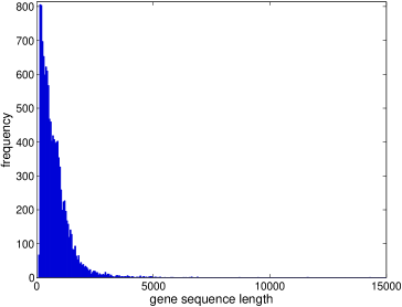
Figure 1: The frequency of 12390 gene sequences length (bp).

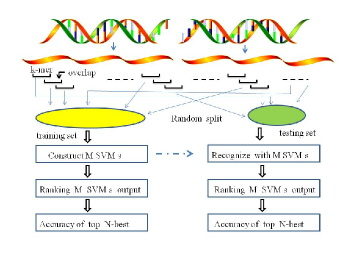
(a)

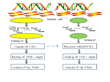
(b)

Figure 2: Framework of SVM with N-best candidates recognition (a) on DI (b) on DII.

To investigate k-mer size of gene sequences, the k-mer sizes of {10, 20, 30, 40, 50} are discussed, and the overlaps of {0, 25%, 50%, 75% } percent of k-mer length are examined. Two types of fragment split strategies are discussed as follows. Taking all genome sequences in each specie into account, for fixed k-mer size , overlap size and split percent , the first strategy (DI) is to segment each genome sequence into k–dimension (bp) sample space, and randomly select the fragments according to given split percent for training data and the rest part (1-split percent) is denoted as testing data(Fig.2(a)). The second strategy (DII) is to randomly split all genome sequences into training and testing parts according to given split percent, then all the sequences in training and testing data sets are mapped into k–dimension sample space separatively according to given k-mer size and overlap size(Fig.2(b)) . DI type data set is obtained along each sequence, although the training and testing data sets are separated according to split percent, the fragments from same sequence still keep the inherent biology information. However, training and testing data sets in DII type never contain this kind of biological information except that these fragments are in same specie property.

After the above segmentation process, all the fragments in the above data sets are treated as dimension-by-dimension segment of genomic sequence. The pattern recognition task on each k–length fragment is called dimension-by-dimension classification.

Taking a further consideration, especially when overlap size is equal to 0, the fragments in training and testing data sets from a same sequence could be treated as two pseudo subsequences of one genomic sequence. As they are randomly selected, the original genomic order information along the same sequence in DI is broken down. The pattern recognition tasks on randomly pseudo genome subsequences in DI and normal order genome subsequences in DII are called sequence-by-sequence classification. While the overlap percent is larger than 0, all the subsequences in DI and DII are pseudo subsequences, the pattern recognition task can still be performed on, it is also named as sequence-by-sequence classification.

In brief, the genomic sequences are mapped into k–dimension sample space, which means the k–bp genomic fragments. To construct the SVM model, the split percents involved in experiments are set as {60%, 80%, 100% }, When split proportion is equal to 100% , the training and testing set are set as same one. For both types of DI and DII, the training sets and testing sets are denoted as $\mathscr{L}(k-mer,overlap,split\ percent)$ and $\mathscr{T}(k-mer,overlap,1-split\ percent)$ respectively. Some main size of samples in $\mathscr{L}(k-mer,overlap,split\ percent)$ and $\mathscr{T}(k-mer,overlap,1-split\ percent)$ involved in experiments are listed in Supplementary Table 1.

2.2 Multi-class SVM

Support Vector Machine (SVM) is a popular statistical learning and machine learning method based on structural risk minimization and VC dimensions theory, and overcomes the dimension disaster of neural network [36]. It has efficient performance and high accuracy in many classification tasks, hence widely used in various information process fields. The traditional SVM is defined for binary classification, the multi-class SVM is defined on binary SVM with one-versus-one max-wins voting strategy or one-versus-all winner-takes-all strategy [37,38]. Suppose the samples data are $\mathscr{D}=\{(x_{i},y_{i})|x_{i}\in R^{k},y_{i}=\pm 1,1\leq i\leq S\}$. Given a nonlinear mapping function $\phi(\cdot)$, the sample data of $x_{i}$ is projected to high dimensional space to obtain well separation of different samples. The standard C-SVM [40] solves

$$\begin{array}[]{ll}\displaystyle{\min_{w,b,\xi}}&\displaystyle(\frac{1}{2}w^{T}w+C\sum_{i=1}^{S}\xi_{i})\\ \displaystyle\mbox{subject to:}&\displaystyle y_{i}(w^{T}\phi(x_{i})+b)\geq 1-\xi_{i},\ \ \ \ \xi_{i}\geq 0,i=1,\cdots,S.\end{array}$$ (1)

where $w,b$ are the parameters of optimal linear hyperplane $f(x)=w^{T}\phi(x)+b$, C is the penalty parameter of the error term. $K(x,x^{\prime})=(\mathbf{x},\mathbf{x^{\prime}})=(\phi(x),\phi(x^{\prime}))$ is the kernel function. The key problem in solving $w$ is involved in the dual problem of above optimization problem and selection of kernel function. The radial basis function(RBF) kernel function is adopted in the experiments, where

$$K(x_{i},x_{j})=\mbox{exp}(-\gamma||x_{i}-x_{j}||^{2}),\gamma>0.$$

Standard LibSVM 3.18 { http://www.csie.ntu.edu.tw/ cjlin/ libsvm/ }is utilized in modeling the fragment vector space, and the parameter range of C-SVM with RBF kernel is $C\times\gamma$ $\in$ {0.0625, 0.125, 0.25, 0.5, 1, 2, 3, 4 } $\times${0.0625, 0.125, 0.25, 0.5, 1, 2, 3, 4 }. Totally 64 parameter choices are employed in experiments.

2.3 Classification Accuracy

For genomic fragment classification, two categories of classification criteria are involved in experiments. The first one is for dimension-by-dimension classification, its aim is to classify the correct accuracy of fragment in k–bp status.

$$\begin{array}[]{ll}\displaystyle frg_{k}=\displaystyle\frac{\#\{correct\ vectors\ for\ right\ class\}}{\#\{total\ vectors\}}\end{array}$$ (2)

The other criterion is to recognize the pseudo subsequence composed of randomly selected fragments from a same sequence for right specie,

$$\begin{array}[]{ll}\displaystyle frs_{k}=\displaystyle\frac{\#\{correct\ sequences\ for\ right\ class\}}{\#\{total\ equences\}}\end{array}$$ (3)

The criteria of $frg_{k}$ and $frs_{k}$ examine the different aspect of gene fragment sequences, both of them address the fragments of partial pieces of genomic sequences.

2.4 Multi–candidate Accuracy

Ranking is a popular technique in genomic analysis and information sciences. In order to show the relationship among the species, the top n $(1\leq n\leq 10)$ ranking classes are considered in the recognition stage according to the top-n probability outputs of multi-class SVM voting. The criteria of classification accuracy with N-best algorithm are revised as follows respectively,

$$\begin{array}[]{ll}\displaystyle frg_{k|n}=\displaystyle\frac{\#\{correct\ vectors\ in\ top-n\ candidates\}}{\#\{total\ vectors\}}\end{array}$$ (4)

$$\begin{array}[]{ll}\displaystyle frs_{k|n}=\displaystyle\frac{\#\{correct\ sequences\ in\ top-n\ candidates\}}{\#\{total\ sequences\}}\end{array}$$ (5)

3 RESULTS

3.1 Accuracy on DI with different k-mer size and Overlap

As there are many combinations of k-mer size, overlap and split percent. Firstly, we investigate the effectiveness of these parameters in a special case that all data is involved in training, that is split percent=100% on DI. And, the case of overlap percent=0 is examined first of all, denoted as $\mathscr{L}(*,0,100\%)$. The dimension–by-dimension recognition experimental results show that on training set $\mathscr{L}(*,0,100\%)$ , the accuracy rates trend highly along the increasing of number of N-candidates and k-mer size value (Fig.3(a), Supplementary Fig.1(a)).

Secondly, we examine the performance on $\mathscr{L}(50,*,100\%)$ with k=50, the accuracy rates increase along number of N-candidates (Fig.3(b)) and decrease along overlap percent (Supplementary Fig.1(b)).

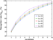
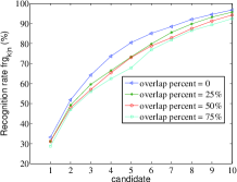
(a)	(b)
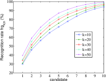
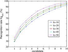
(c)	(d)
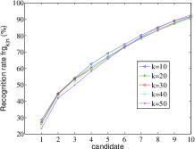
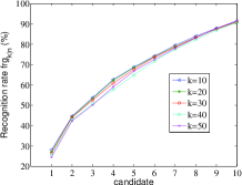
(e)	(f)

Figure 3: Dimension-by-Dimension recognition rates on DI along multi–candidates. (a) $\mathscr{L}(*,0,100\%)$ (b) $\mathscr{L}(50,*,100\%)$ (c) $\mathscr{L}(*,0,60\%)$ (d) $\mathscr{L}(*,0,80\%)$ (e) $\mathscr{T}(*,0,40\%)$ (f)$\mathscr{T}(*,0,20\%)$.

Thirdly, we perform multi-class SVM with N-best algorithm on DI with split percent=60% and 80% cases. In the dimension-by-dimension case, in training sets, the accuracy rates increase along number of candidates (Fig.3(c)(d)) and k-mer size (Supplementary Fig.1(c)(d)). While in testing sets, the accuracy rates increase along number of candidates (Fig.3(e)(f)) and slightly decrease along k-mer size (Supplementary Fig.1(e)(f)) especial in low candidate values.

Fourthly, the multi-class SVM with N-best algorithm are performed in sequence-by-sequence cases of $\mathscr{L}(*,0,100\%)$ and $\mathscr{L}(50,*,100\%)$, the same conclusions hold as dimension-by-dimension cases (Fig.4(a)(b),Supplementary Fig.2(a)(b)). At same time, the accuracy rate of recognition in pseudo sequence-by-sequence form is more higher than in dimension-by-dimension fragment form.

Fifthly, in the sequence-by-sequence cases on DI with split percent=60% and 80% cases, the accuracy rates increase along number of candidates (Fig.4(c)(d)), but will not do so along k-mer size (Supplementary Fig.2(c)(d)) in training sets. The accuracy rates increase from 10 to 30 of k-mer size from top-1 to top-6 candidate cases, however, decrease in top-10 case within k-mer size from 10 to 30 (Supplementary Fig.2(c)(d)). From 30 to 50 k-mer size, the accuracy rates decrease from top-2 to top-10 in $\mathscr{L}(*,0,60\%)$ (Supplementary Fig.2(c)) and from top-3 to top-10 in $\mathscr{T}(*,0,80\%)$ (Supplementary Fig.2(d)). These experimental results demonstrate the tendency of accuracy rates with k-mer size and top-n candidates. In each fixed k-mer size, the principle that the larger the number of top-n candidates, the higher the accurate rates still holds. While, in testing data, The accuracy rates under each fixed k-mer size increases along top-n candidates (Fig.4(e)(f)), however, the accuracy rates under each fixed top-n candidates decreases along k-mer size (Supplementary Fig.2(e)(f)). The appropriate choice of k-mer size for genomic fragments and sequences predictions would be 10.

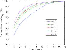
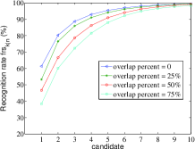
(a)	(b)
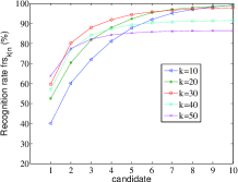
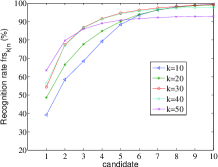
(c)	(d)
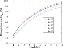
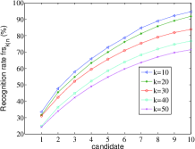
(e)	(f)

Figure 4: Sequence–by-sequence recognition rates on DI along multi–candidates. (a) $\mathscr{L}(*,0,100\%)$ (b) $\mathscr{L}(50,*,100\%)$ (c) $\mathscr{L}(*,0,60\%)$ (d) $\mathscr{L}(*,0,80\%)$ (e) $\mathscr{T}(*,0,40\%)$ (f)$\mathscr{T}(*,0,20\%)$.

Sixthly, as to the overlap problem on DI with split percent=60% and 80% for training and testing cases separatively, we give the discussion in the case of 50 k-mer size data sets. In the dimension-by-dimension case, the performances on training sets and testing sets are different. In training sets, the accuracy rates under each overlap percent increase along the top-n candidates (Fig.5(a)(b)) , and the accuracy rates under each top-n candidates decrease along the overlap percent (Supplementary Fig.3(a)(b)). In testing sets, the accuracy rates under each overlap percent increase along the top-n candidates (Fig.5(c)(d)), and the accuracy rates under each top-n candidates are not precisely synchronized with the increasing of overlap percent (Supplementary Fig.3(c)(d)), in low top-n case, there are slightly enhancement, but do not hold in large top-n cases.

Seventhly, in sequence-by-sequence cases of 50 k-mer size data sets with split percent=60% and 80% for training and testing sets separatively on DI, for fixed overlap percent, the accuracy rates increases on both training (Fig.6(a)(b)) and testing data sets (Fig.6(c)(d)). Given top-n candidates, the accuracy rates perform different along overlap percent. In training sets, the accuracy rates decrease along low top-n candidates cases and increase in high top-n candidates cases (Supplementary Fig.4(a)(b)). But, in testing data, the accuracy rates increase along overlap percent (Supplementary Fig.4(c)(d)). The above experimental results show that overlap optimization is somewhat complicate in training and testing sets. The optimized overlap would be the balance between training and testing sets.

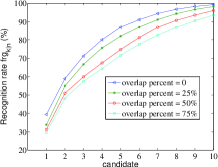
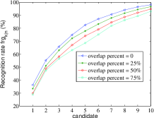
(a)	(b)
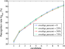
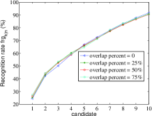
(c)	(d)

Figure 5: dimension-by-dimension recognition rates on DI. (a) $\mathscr{L}(50,*,60\%)$ (b) $\mathscr{L}(50,*,80\%)$ (c) $\mathscr{T}(50,*,40\%)$ (d) $\mathscr{T}(50,*,20\%)$.

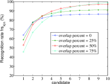
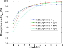
(a)	(b)
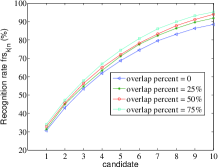
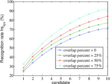
(c)	(d)

Figure 6: sequence-by-sequence recognition rates on DI. (a) $\mathscr{L}(50,*,60\%)$ (b) $\mathscr{L}(50,*,80\%)$ (c) $\mathscr{T}(50,*,40\%)$ (d) $\mathscr{T}(50,*,20\%)$.

The experimental results on DI above show that, on training sets, the high k-mer size is preferred, on testing sets, the relative low k-mer will obtain relative good performance. As to the overlap percent, the sequence-by-sequence recognition on testing data sets would prefer higher value of overlap. All of the experimental results of this section are listed in Supplementary Table 2 and Supplementary Table 3.

3.2 Accuracy on DII with different k-mer size

This section we will show the performance of multi-class SVM with N-best algorithm on DII, which is different from DI in biology information, where experiments on DI would be treated as a kind of gene prediction, and the experiments on DII would be treated as a kind of gene category. The experimental results on data sets with split percents 60% and 80% are investigated. All the experimental results of dimension-by-dimension cases are listed in Supplementary Table 4, and sequence-by-sequence cases are listed in Supplementary Table 5.

Firstly, in dimension-by-dimension case, the accuracy rates increase along top-n candidates and k-mer size (Fig.7(a)(b)(c)(d)) on training data sets,, while the accuracy rates on testing data sets increase along top-n candidates and slightly decrease along k-mer size in top-n candidates case, in other top-n case, the fluctuation of accuracy rate along k-mer size is not distinctive (Supplementary Fig.5(a)(b)(c)(d)).

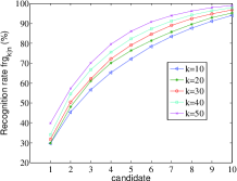
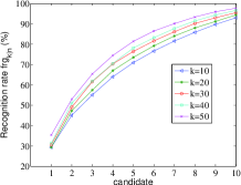
(a)	(b)
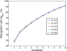
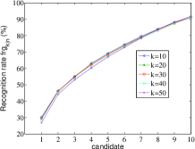
(c)	(d)

Figure 7: dimension-by-dimension recognition rates on DII. (a) $\mathscr{L}(*,0,60\%)$ (b) $\mathscr{L}(*,0,80\%)$ (c) $\mathscr{T}(*,0,40\%)$ (d) $\mathscr{T}(*,0,20\%)$.

Secondly, in sequence-by-sequence cases, the accuracy rates increase along both top-n candidates and k-mer size on training data sets (Fig.8(a)(b)(c)(d)), while the accuracy rates increase along top-n candidates and slightly decrease along k-mer size on testing data sets (Supplementary Fig.6(a)(b)(c)(d)).

Again, the appropriate selection of k-mer size on DII type data sets would be 10. This conclusion is also helpful to model metagenomic sequences with HMM though it is difficult for HMM framework to examine the high dimensional k-mer size cases.

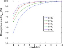
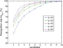
(a)	(b)
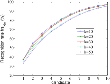
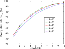
(c)	(d)

Figure 8: sequence-by-sequence recognition rates on DII. (a) $\mathscr{L}(*,0,60\%)$ (b) $\mathscr{L}(*,0,80\%)$ (c) $\mathscr{T}(*,0,40\%)$ (d) $\mathscr{T}(*,0,20\%)$.

Moreover, from all the experimental results on split percent 60% and 80%, the principles along parameters of overlap and k-mer size have almost the same tendency, which is also provide the reasonable explanations of our models and performance. Regardless of DI and DII, the fact that 10 k-mer size with top-10 candidates can achieve high recognition rates demonstrates that the centroid marker family genomic sequences of all microbial would be highly discriminated with the toleration of confusion of 10 species among the 17 species within the multi-class SVM with N-best algorithm framework, the confusion is mainly caused by the similarities among species measured by multi-class SVM model in the view of evolution[55,56].

4 DISCUSSION

We develop the multi-class SVM based N-best algorithm on microbial species classification, realize the true sense of fragment classification of genomic sequences without preprocessing, and discuss the effectiveness of k-mer size,overlap and split percent. The genome sequences of maker family from all microbial on MetaRef are treated as time series and employed in experiments with different lengths. Generally, the experimental results on the given range of SVM parameters grids show that the larger the k-mer size from 10 to 50, the higher the accuracy rates on training sets. The conclusions on testing sets are reverse. The overlap of fragments also takes effect on different data sets. In the view of prediction, the low overlap is recommended. Furthermore, N-best algorithm shows that top-10 candidates would provide good experimental results on both dimension-by-dimension and sequence-by-sequence recognition tasks. The experiments are designed only based on the {A,C,T,G} information along genomic sequences, if the detail 3-D genomic structure information or biology information are available, the prediction accuracy rates would be higher. Though the multi-class SVM with N-best algorithm and feature selection are constructed for challenging fragment classification, it would be applied to cancer diagnose of genomic fragments in future. And, how to overcome the time–consumption and memory storage of SVM and propose new kernel SVM are our future research interests. Finally, great improvement of top-1 classification accuracy is also our research goal in microbial genomic analysis.

5 ACKNOWLEDGEMENTS

This paper is partially supported by CHINA SCHOLARSHIP COUNCIL (No. 201303070216), 863 Project of China (2008AA02Z306), it was finished while I visited University of Southern California from March.2014 to Feb.2015.

5.0.1 Conflict of interest statement.

None declared.

Table 1: Vector number of marker gene database with different dimension (k-bp).

DI
Dimension	Overlap percent
	0	25%	50%	75%
10	921139	1149824	1835989	3055903
20	457482	608681	908749	1811209
30	302566	393194	598807	1118850
40	225659	298783	445092	883969
50	179205	233895	352308	671869
DII
Dimension	Split percent (training/testing)
	60%	40%	80%	20%
10	552213	368926	739042	182097
20	274266	183216	367056	90426
30	181389	121177	242767	59799
40	135302	90357	181062	44597
50	107420	71785	143791	35414

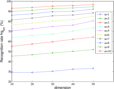
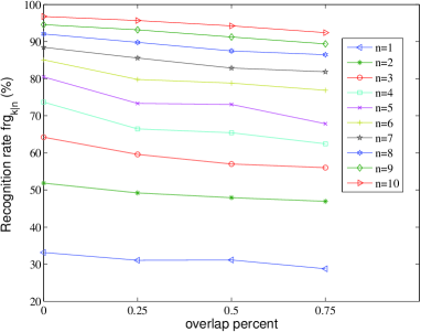
(a)	(b)
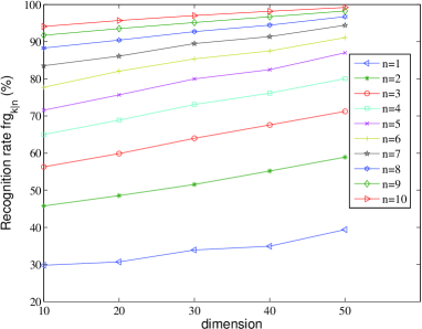
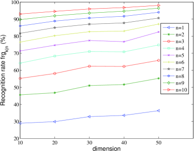
(c)	(d)
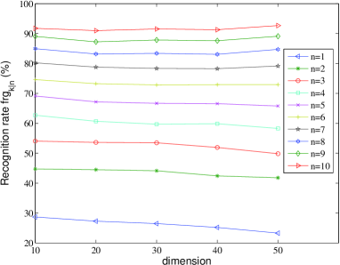
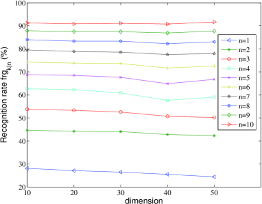
(e)	(f)

Dimension-by-Dimension recognition rates on DI. (a) $\mathscr{L}(*,0,100\%)$ (b) $\mathscr{L}(50,*,100\%)$ (c) $\mathscr{L}(*,0,60\%)$ (d) $\mathscr{L}(*,0,80\%)$ (e) $\mathscr{T}(*,0,40\%)$ (f)$\mathscr{T}(*,0,20\%)$.

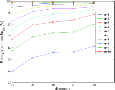
(a)	(b)
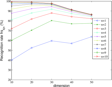
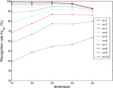
(c)	(d)
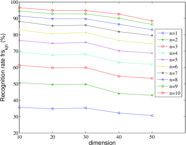
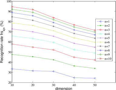
(e)	(f)

Sequence–by–sequence recognition rates on DI. (a) $\mathscr{L}(*,0,100\%)$ (b) $\mathscr{L}(50,*,100\%)$ (c) $\mathscr{L}(*,0,60\%)$ (d) $\mathscr{L}(*,0,80\%)$ (e) $\mathscr{T}(*,0,40\%)$ (f)$\mathscr{T}(*,0,20\%)$.

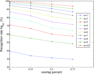
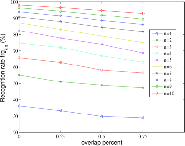
(a)	(b)
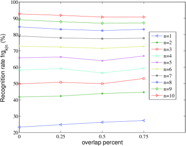
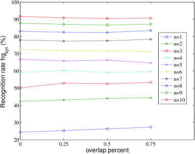
(c)	(d)

Dimension–by–dimension recognition rates on DI. (a) $\mathscr{L}(50,*,60\%)$ (b) $\mathscr{L}(50,*,80\%)$ (c) $\mathscr{T}(50,*,40\%)$ (d) $\mathscr{T}(50,*,20\%)$.

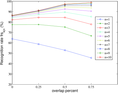
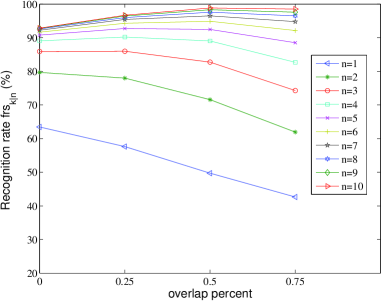
(a)	(b)
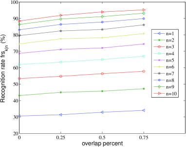
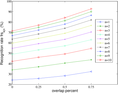
(c)	(d)

Sequence–by–sequence recognition rates on DI. (a) $\mathscr{L}(50,*,60\%)$ (b) $\mathscr{L}(50,*,80\%)$ (c) $\mathscr{T}(50,*,40\%)$ (d) $\mathscr{T}(50,*,20\%)$.

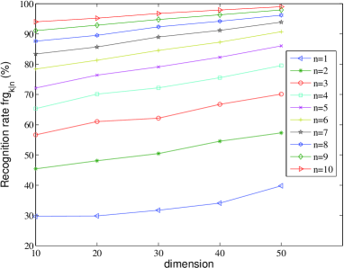
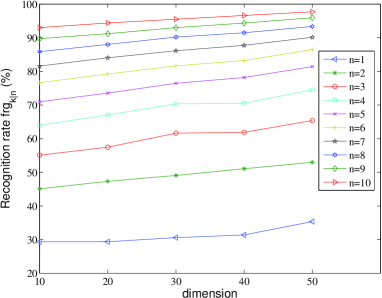
(a)	(b)
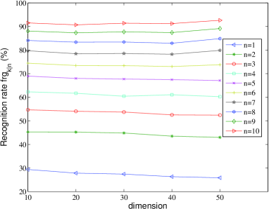
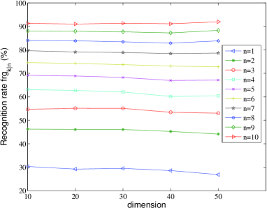
(c)	(d)

Dimension–by–dimension recognition rates on DII . (a) $\mathscr{L}(*,0,60\%)$ (b) $\mathscr{L}(*,0,80\%)$ (c) $\mathscr{T}(*,0,40\%)$ (d) $\mathscr{T}(*,0,20\%)$.

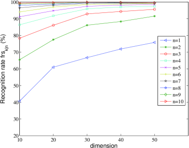
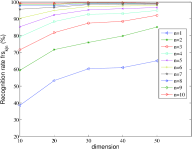
(a)	(b)
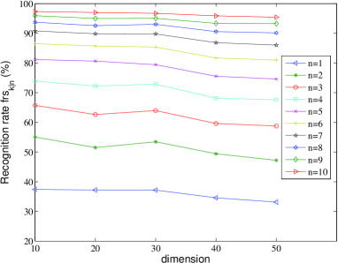
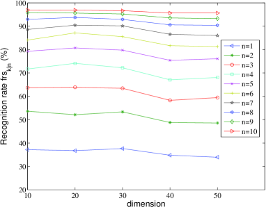
(c)	(d)

Sequence–by–sequence recognition rates on DII. (a) $\mathscr{L}(*,0,60\%)$ (b) $\mathscr{L}(*,0,80\%)$ (c) $\mathscr{T}(*,0,40\%)$ (d) $\mathscr{T}(*,0,20\%)$.

Table 2: Maximum accuracy rates of dimension-by-dimension recognition with SVM and top N-Best on DI.

Data set	N–candidate
	1	2	3	4	5	6	7	8	9	10
$\mathscr{L}(10,0,100\%)$	29.1524	45.3499	55.1381	63.9802	70.5578	76.3853	81.4770	86.0207	89.7962	92.9417
$\mathscr{L}(20,0,100\%)$	29.1290	46.7605	57.4512	65.9442	72.5504	78.3019	83.2321	87.4885	90.9828	93.8046
$\mathscr{L}(30,0,100\%)$	30.2417	48.5501	59.5906	67.4187	74.8785	80.3749	85.4805	89.5094	92.7047	95.1597
$\mathscr{L}(40,0,100\%)$	32.3072	50.1270	62.1664	70.1953	76.2544	81.7982	86.2868	89.9982	93.2974	95.6939
$\mathscr{L}(50,0,100\%)$	33.1408	51.8390	64.2131	73.6849	80.4710	85.0886	88.4445	92.0622	94.5749	96.7707
$\mathscr{L}(50,0.25,100\%)$	31.0661	49.1964	59.6015	66.4508	73.3321	79.8003	85.5709	89.7882	93.1794	95.6673
$\mathscr{L}(50,0.5,100\%)$	31.1293	47.9385	57.0064	65.4158	73.0545	78.7950	82.8590	87.4695	91.2446	94.2269
$\mathscr{L}(50,0.75,100\%)$	28.7537	46.9359	56.0094	62.4396	67.8412	76.8814	81.8509	86.4579	89.3755	92.4086
$\mathscr{L}(10,0,80\%)$	28.9219	45.5890	55.2286	64.1692	71.3453	76.5182	81.6939	86.0141	89.7028	93.0153
$\mathscr{L}(20,0,80\%)$	29.8525	46.8040	58.0903	68.3442	74.6969	80.2725	85.0012	88.8769	91.9582	94.5587
$\mathscr{L}(30,0,80\%)$	32.8037	50.9962	62.3726	71.0052	77.4849	82.6210	87.0528	90.6602	93.5443	95.9695
$\mathscr{L}(40,0,80\%)$	33.5453	51.6201	62.2330	70.8199	76.7607	82.9937	87.7732	91.6892	94.6637	96.8024
$\mathscr{L}(50,0,80\%)$	36.2889	55.2549	65.8190	74.8511	82.4900	87.1315	90.6297	94.0369	96.4533	98.0879
$\mathscr{L}(50,0.25,80\%)$	33.4600	51.0611	63.0256	72.2075	77.8655	83.2365	87.9323	91.5702	94.4105	96.6420
$\mathscr{L}(50,0.50,80\%)$	29.8364	48.9057	58.1688	67.0047	74.0874	79.0414	84.4936	88.6204	91.9367	94.8254
$\mathscr{L}(50,0.75,80\%)$	28.9125	47.4129	56.5023	63.1323	68.6258	75.1206	81.8824	86.2010	89.3410	93.0019
$\mathscr{T}(10,0,20\%)$	28.1011	44.6525	53.7493	62.6669	68.7712	74.2429	79.5064	83.9734	87.8928	91.2690
$\mathscr{T}(20,0,20\%)$	27.1238	44.2305	53.3159	62.3020	68.5094	73.8141	78.8983	83.3520	87.5116	90.8618
$\mathscr{T}(30,0,20\%)$	26.4781	44.0914	52.5489	60.8670	67.6340	73.6352	78.5645	83.3591	87.4677	91.0892
$\mathscr{T}(40,0,20\%)$	25.5126	42.7923	50.7391	57.6458	64.8765	71.6992	77.5538	82.2442	86.8907	90.7711
$\mathscr{T}(50,0,20\%)$	24.4188	42.2969	50.1801	59.0578	66.7598	72.5435	77.9893	83.0920	87.7441	91.6783
$\mathscr{T}(50,0.25,20\%)$	25.2634	43.1037	52.8523	60.3333	65.7691	71.7519	77.3482	82.4728	87.0851	90.8430
$\mathscr{T}(50,0.50,20\%)$	26.3453	44.0362	52.5299	59.0685	66.2043	71.7062	77.5346	82.3529	86.6402	90.4444
$\mathscr{T}(50,0.75,20\%)$	27.3373	44.3945	53.3592	59.5510	64.6706	71.2024	78.3791	83.4635	87.2125	90.6695
$\mathscr{L}(10,0,60\%)$	29.8095	45.7840	56.3059	64.9796	71.5621	77.7058	83.5297	88.3057	91.7147	94.1014
$\mathscr{L}(20,0,60\%)$	30.6973	48.5402	59.8552	68.8960	75.6688	82.0383	86.1187	90.4233	93.5281	95.6958
$\mathscr{L}(30,0,60\%)$	33.9040	51.5536	63.9864	73.0764	79.9770	85.3750	89.5019	92.7104	95.1563	97.0519
$\mathscr{L}(40,0,60\%)$	34.9225	55.1855	67.5837	76.1416	82.4520	87.4890	91.3761	94.4557	96.7062	98.1885
$\mathscr{L}(50,0,60\%)$	39.3829	58.9222	71.2244	80.0714	87.0090	91.0924	94.4168	96.7459	98.2642	99.2233
$\mathscr{L}(50,0.25,60\%)$	33.8457	55.0146	66.6992	75.6584	82.0342	87.0414	91.1657	94.3555	96.6417	98.1922
$\mathscr{L}(50,0.50,60\%)$	31.2826	50.9855	59.9542	67.4814	74.7800	81.2390	86.9697	90.7208	93.5934	96.0711
$\mathscr{L}(50,0.75,60\%)$	29.5668	48.1559	57.5237	64.3312	71.6415	77.5680	82.5913	86.9179	90.5514	93.5667
$\mathscr{T}(10,0,40\%)$	28.6860	44.7459	54.0663	62.7004	69.1209	74.6020	80.2309	84.9403	89.0569	91.7479
$\mathscr{T}(20,0,40\%)$	27.2974	44.4829	53.6333	60.6738	67.1645	73.2349	78.7768	83.1719	87.2416	90.9932
$\mathscr{T}(30,0,40\%)$	26.4721	44.1347	53.4889	59.7083	66.6915	72.8363	78.3563	83.3982	87.8438	91.5343
$\mathscr{T}(40,0,40\%)$	25.2008	42.4063	51.9196	59.8656	66.5702	72.9194	78.2758	83.0555	87.6245	91.2929
$\mathscr{T}(50,0,40\%)$	23.2928	41.7797	49.8286	58.2750	65.7790	72.9532	79.1590	84.7130	89.1239	92.6863
$\mathscr{T}(50,0.25,40\%)$	24.8183	42.3461	50.7740	59.1511	66.2693	72.3535	77.9521	83.2761	87.9005	91.8124
$\mathscr{T}(50,0.50,40\%)$	26.2837	43.8785	49.9088	56.4861	63.9817	71.5918	77.5077	82.4559	86.9606	90.7753
$\mathscr{T}(50,0.75,40\%)$	27.3154	44.6684	53.1084	59.2998	66.9273	72.7711	77.8036	83.2448	87.1742	90.7759

Table 3: Maximum accuracy rates of sequence-by-sequence recognition with SVM and top N-Best on DI.

Data set	N–candidate
	1	2	3	4	5	6	7	8	9	10
$\mathscr{L}(10,0,100\%)$	39.4915	57.4576	67.2639	75.4722	82.6634	89.2010	95.0202	97.5706	98.7571	99.3624
$\mathscr{L}(20,0,100\%)$	51.3156	69.2575	79.3462	86.0371	90.8878	94.2050	96.1582	97.6513	98.5876	99.1768
$\mathscr{L}(30,0,100\%)$	55.9726	72.7441	82.1065	89.0395	93.6481	95.9241	97.3204	98.3858	98.9266	99.3866
$\mathscr{L}(40,0,100\%)$	56.4568	73.4544	83.7369	90.1291	93.7611	95.9887	97.5545	98.5069	99.0073	99.3947
$\mathscr{L}(50,0,100\%)$	61.2994	80.2663	88.6844	92.8975	95.4237	96.9976	98.0468	98.7006	99.0395	99.3140
$\mathscr{L}(50,0.25,100\%)$	53.2526	76.5214	85.9564	91.0412	94.1001	96.1824	97.4173	98.3293	98.9346	99.2655
$\mathscr{L}(50,0.5,100\%)$	46.6344	66.6182	78.6683	86.2308	90.9524	94.0678	96.2228	97.5383	98.4262	99.0557
$\mathscr{L}(50,0.75,100\%)$	38.3939	60.1049	72.2680	81.5335	87.9984	92.1872	94.9314	96.5698	97.6755	98.2728
$\mathscr{L}(10,0,80\%)$	39.1364	58.4262	68.4504	79.2575	88.3777	93.5109	96.3842	97.9903	98.8943	99.4350
$\mathscr{L}(20,0,80\%)$	48.6037	66.5456	77.6513	84.8265	90.0646	93.8983	96.2550	97.7805	98.6602	99.0234
$\mathscr{L}(30,0,80\%)$	54.3906	77.4173	86.8039	91.6303	94.6086	96.2308	97.4011	98.2405	98.8701	99.2494
$\mathscr{L}(40,0,80\%)$	56.3600	77.0541	86.5456	91.3882	94.1727	95.8031	96.8119	97.3527	97.6755	97.8692
$\mathscr{L}(50,0,80\%)$	63.4544	79.6772	85.9161	89.0638	90.7667	91.6546	92.2195	92.5989	92.7603	92.8571
$\mathscr{L}(50,0.25,80\%)$	57.6352	77.9903	85.9887	90.2018	92.7441	94.2776	95.4479	95.9726	96.4487	96.6747
$\mathscr{L}(50,0.50,80\%)$	49.7256	71.5900	82.7199	89.0315	92.4697	94.8910	96.4972	97.5868	98.3212	98.8378
$\mathscr{L}(50,0.75,80\%)$	42.6312	61.9290	74.2938	82.6877	88.5149	92.1388	94.7700	96.5052	97.5868	98.5149
$\mathscr{T}(10,0,20\%)$	33.4221	47.6433	57.8935	65.8596	72.8491	78.6441	84.7215	88.8539	92.1711	94.5924
$\mathscr{T}(20,0,20\%)$	31.5658	45.4641	54.8265	63.3495	69.9596	76.1501	81.2510	85.7304	89.0799	91.7998
$\mathscr{T}(30,0,20\%)$	30.9847	42.3648	52.1630	59.4754	65.6013	70.9201	75.3511	79.0718	81.8967	83.8337
$\mathscr{T}(40,0,20\%)$	24.7700	36.3519	44.8426	52.2841	58.5714	63.8902	68.2647	71.7918	74.6893	76.7232
$\mathscr{T}(50,0,20\%)$	24.2131	33.9387	42.2115	49.0073	54.7054	59.6691	63.6077	66.9814	69.6529	71.4205
$\mathscr{T}(50,0.25,20\%)$	25.6739	36.9492	46.0856	53.2203	59.1687	64.2938	68.5069	72.2841	74.8830	76.9976
$\mathscr{T}(50,0.50,20\%)$	28.3132	40.5004	49.2978	57.1186	63.3656	69.1525	74.0032	77.9903	81.3801	84.1727
$\mathscr{T}(50,0.75,20\%)$	32.3648	43.7046	54.5763	62.9863	70.4358	76.7635	82.0420	86.5214	90.0242	92.7441
$\mathscr{L}(10,0,60\%)$	40.0726	60.2098	72.0420	81.1784	87.7401	91.9774	95.1574	97.0299	98.3132	99.2010
$\mathscr{L}(20,0,60\%)$	52.5424	70.4439	81.8321	87.9984	92.3487	95.4076	97.0944	97.9903	98.5391	98.9911
$\mathscr{L}(30,0,60\%)$	59.6449	80.2906	87.9822	91.8886	94.4794	95.8192	96.6586	97.2801	97.6513	97.8370
$\mathscr{L}(40,0,60\%)$	56.9895	76.9734	84.2696	87.4011	89.2655	90.3148	90.8232	91.1703	91.3479	91.4366
$\mathscr{L}(50,0,60\%)$	63.8257	77.4980	82.1711	84.3099	85.2785	85.8273	86.1259	86.3519	86.4084	86.4326
$\mathscr{L}(50,0.25,60\%)$	58.7571	77.5948	84.3987	87.2801	88.7732	89.8467	90.4923	90.7829	91.0089	91.0734
$\mathscr{L}(50,0.50,60\%)$	52.8733	75.1816	84.4068	89.5319	92.5504	94.4310	95.6659	96.5214	96.9976	97.2074
$\mathscr{L}(50,0.75,60\%)$	45.4883	66.6990	77.7966	85.2220	90.4681	93.6804	95.7143	97.0218	98.1679	98.8216
$\mathscr{T}(10,0,40\%)$	35.6336	50.7506	61.3156	69.5238	76.5698	82.9701	88.1921	91.4851	94.4391	96.5214
$\mathscr{T}(20,0,40\%)$	34.7538	49.5480	59.8305	67.5787	74.6812	80.5650	85.4964	89.7498	92.8410	94.9314
$\mathscr{T}(30,0,40\%)$	35.2623	49.7094	59.9274	68.0307	75.3592	81.3963	85.8596	89.6852	92.7603	94.7619
$\mathscr{T}(40,0,40\%)$	32.1792	44.0597	54.6166	63.0670	70.2018	76.5133	81.8563	86.3842	90.0565	92.6069
$\mathscr{T}(50,0,40\%)$	30.5892	43.0508	53.3737	61.8967	68.7248	74.4713	79.5480	83.0831	86.3115	88.4181
$\mathscr{T}(50,0.25,40\%)$	31.3721	45.0202	54.7619	63.3737	71.1461	77.5787	82.3648	86.3519	89.6287	91.8563
$\mathscr{T}(50,0.50,40\%)$	32.8814	45.7224	56.3519	64.9798	72.0097	78.2324	83.2768	87.7643	91.1299	93.9629
$\mathscr{T}(50,0.75,40\%)$	34.0113	47.1832	57.7805	66.9895	74.4310	80.7425	86.0775	89.9031	93.1638	95.2139

Table 4: Maximum accuracy rates of dimension-by-dimension recognition with SVM and top N-Best on DII.

Data set	N–candidate
	1	2	3	4	5	6	7	8	9	10
$\mathscr{L}(10,0,80\%)$	29.3438	45.0915	55.0882	63.9969	70.9697	76.6488	81.5802	85.8802	89.7327	93.0207
$\mathscr{L}(20,0,80\%)$	29.3552	47.3296	57.4534	67.0448	73.5479	79.2198	84.0477	88.0165	91.2125	94.4000
$\mathscr{L}(30,0,80\%)$	30.5824	49.0668	61.6422	70.3588	76.4742	81.6552	86.1316	90.2112	93.0098	95.5282
$\mathscr{L}(40,0,80\%)$	31.3881	51.0709	61.8799	70.5493	78.1694	83.2345	87.7401	91.4764	94.3804	96.6437
$\mathscr{L}(50,0,80\%)$	35.3590	52.9908	65.4033	74.5144	81.4203	86.4866	90.1496	93.3702	95.9525	97.7147
$\mathscr{T}(10,0,20\%)$	30.3086	46.2396	54.6489	63.0856	69.1697	74.5647	79.6372	83.9981	88.0772	91.2766
$\mathscr{T}(20,0,20\%)$	29.2051	46.0697	55.1003	62.7021	68.8629	74.2264	79.0846	83.8409	87.8995	90.9838
$\mathscr{T}(30,0,20\%)$	29.5038	46.0827	55.0661	62.0462	68.2403	73.6785	78.8558	83.4111	87.6787	91.3259
$\mathscr{T}(40,0,20\%)$	28.5826	45.2497	53.3937	60.1408	66.9529	73.0946	78.3932	82.8464	87.2144	91.0958
$\mathscr{T}(50,0,20\%)$	26.8566	44.1238	53.0242	60.4083	67.1062	72.7848	78.6045	83.8256	88.2956	91.9439
$\mathscr{L}(10,0,60\%)$	29.6971	45.4136	56.6370	65.3096	72.1330	78.4000	83.3930	87.6122	91.1014	94.0061
$\mathscr{L}(20,0,60\%)$	29.8586	48.0800	61.0491	70.1224	76.3722	81.3218	85.6909	89.5342	92.9098	95.2152
$\mathscr{L}(30,0,60\%)$	31.7213	50.4551	62.1493	72.1824	79.1184	84.5586	88.9960	92.3518	94.7919	96.7793
$\mathscr{L}(40,0,60\%)$	34.0660	54.5520	66.7263	75.5318	82.2952	87.2818	91.1775	94.1952	96.3349	97.9076
$\mathscr{L}(50,0,60\%)$	39.8064	57.2994	70.1210	79.5504	86.0678	90.7522	93.9192	96.1972	97.9287	98.9955
$\mathscr{T}(10,0,40\%)$	29.4029	45.2738	54.6847	62.3008	68.9545	74.4504	79.6967	84.0683	88.0486	91.5156
$\mathscr{T}(20,0,40\%)$	27.8420	45.2155	54.0493	61.6988	67.9848	73.4767	78.4582	83.3492	87.3313	90.7006
$\mathscr{T}(30,0,40\%)$	27.4326	44.8435	53.7272	60.4323	67.7084	73.4091	78.5520	83.4251	87.7196	91.3985
$\mathscr{T}(40,0,40\%)$	26.3455	43.5107	52.5305	61.0567	67.4679	73.0270	78.2297	82.8868	87.4177	91.2270
$\mathscr{T}(50,0,40\%)$	25.8717	42.9881	52.4357	60.2326	67.0739	73.7870	79.8593	84.8659	89.1454	92.6294

Table 5: Maximum accuracy rates of sequence-by-sequence recognition with SVM and top N-Best on DII.

Data set	N–candidate
	1	2	3	4	5	6	7	8	9	10
$\mathscr{L}(10,0,80\%)$	38.5928	59.4387	71.6031	79.3257	85.3321	90.3392	95.7601	97.8397	98.6473	99.2833
$\mathscr{L}(20,0,80\%)$	53.3313	71.7141	81.8393	88.3909	92.3178	95.0333	96.9110	97.8397	98.6574	99.2631
$\mathscr{L}(30,0,80\%)$	60.3170	76.0044	87.4823	92.7519	95.3463	97.3047	98.4757	98.9804	99.4246	99.7072
$\mathscr{L}(40,0,80\%)$	61.0337	79.8506	88.5524	93.1052	96.0933	97.6782	98.6170	99.1016	99.4044	99.6164
$\mathscr{L}(50,0,80\%)$	65.0616	85.1605	92.1260	95.0030	96.7494	97.8498	98.6069	99.1016	99.2227	99.3438
$\mathscr{T}(10,0,20\%)$	37.1981	53.6232	63.6876	71.6989	79.2673	84.0580	88.6071	92.9549	95.8132	96.9807
$\mathscr{T}(20,0,20\%)$	36.7552	52.1337	63.8889	74.1143	80.7166	87.1578	90.4589	93.7601	95.6119	96.9002
$\mathscr{T}(30,0,20\%)$	37.6409	53.3414	63.4461	72.2222	79.7504	85.5475	90.1369	92.9147	95.2496	96.6586
$\mathscr{T}(40,0,20\%)$	34.7826	48.7923	58.2931	67.0692	75.4026	81.6828	86.5539	90.5797	93.5588	95.6522
$\mathscr{T}(50,0,20\%)$	33.9372	48.5910	59.4605	68.0757	76.0870	81.2802	86.0306	90.3784	93.2770	95.6522
$\mathscr{L}(10,0,60\%)$	40.6839	65.4685	78.3522	86.3893	91.1820	94.0899	96.6074	98.0075	98.8422	99.3538
$\mathscr{L}(20,0,60\%)$	60.9989	77.4906	86.1201	91.7744	94.8438	96.9844	98.0614	98.7076	99.1788	99.6904
$\mathscr{L}(30,0,60\%)$	66.7340	86.1470	92.9052	95.9208	97.4690	98.5460	99.2057	99.5961	99.7981	99.9192
$\mathscr{L}(40,0,60\%)$	71.9171	88.3549	94.3726	97.0382	98.1556	98.8018	99.2326	99.5019	99.6634	99.7711
$\mathscr{L}(50,0,60\%)$	75.8481	91.5590	95.6247	97.3748	98.4787	99.0980	99.3134	99.4884	99.5019	99.5288
$\mathscr{T}(10,0,40\%)$	37.4244	55.0786	65.7195	73.9218	81.1769	86.5175	90.7900	93.7324	95.9492	97.3398
$\mathscr{T}(20,0,40\%)$	37.2229	51.5316	62.6562	72.2289	80.6328	85.7316	89.8428	92.5836	95.0020	97.0173
$\mathscr{T}(30,0,40\%)$	37.1826	53.4462	63.9863	72.8537	79.4236	85.3688	89.8025	93.0270	95.0625	96.7352
$\mathscr{T}(40,0,40\%)$	34.6030	49.4156	59.6131	68.1378	75.5341	81.7009	86.8601	90.5885	93.3495	95.9089
$\mathscr{T}(50,0,40\%)$	33.1520	47.2189	58.7666	67.6340	74.6070	80.9754	86.0339	90.1451	93.2890	95.4454

References

- [1] Ku CS,Roukos DH.(2013) From next-generation sequencing to nanopore sequencing technology: paving the way to personalized genomic medicine. Expert Rev. Med. Devices, 10(1),1–6.
- [2] Lipman DJ,Pearson WR.(1985) Rapid and sensitive protein similarity searches. Science, 227 (4693), 1435–1441.
- [3] Pearson WR,Lipman DJ.(1988) Improved tools for biological sequence comparison. Proc. Natl. Acad. Sci. USA, 85(8), 2444–2448.
- [4] Altschul SF,Gish W,Miller W,Myers EW,Lipman DJ.(1990) Basic local alignment search tool. Journal of Molecular Biology, 215, 403–410.
- [5] Krogh A,Mian IS,Haussler D.(1994) A hidden Markov model that finds genes in E. coli DNA. Nucleic Acids Research, 22, 4768–4778.
- [6] Burge C,Karlin S.(1997) Prediction of complete gene structures in human genomic DNA. Journal of Molecular Biology, 268, 78–94.
- [7] Salzberg SL,Delcher AL,Kasif S,White O.(1998) Microbial gene identification using interpolated Markov models. Nucleic Acids Research, 26(2), 544-548.
- [8] Lukashin AV,Borodovsky M.(1998) GenMark.hmm: new solutions for gene finding. Nucleic Acids Research, 26(4), 1107-1115.
- [9] Pedersen JS,Hein J.(2003) Gene finding with a hidden Markov model of genome structure and evolution. Bioinformatics, 19(2), 219-227.
- [10] Cawley SL,Pachter L.(2003) HMM sampling and applications to gene conding and alternative splicing. Bioinformatics, 19 Suppl. 2: ii36–ii41.
- [11] DePristo MA,Banks E,Poplin RE,Garimella KV,Maguire JR,Hartl C,Philippakis AA,del Angel G,Rivas MA, Hanna M, et al.(2011) A framework for variation discovery and genotyping using next-generation DNA sequencing data. Nat Genet. , 43(5), 491–498.
- [12] Abubucker S,Segata N,Goll J,Schubert AM,Izard J,Cantarel BL,Rodriguez-Mueller B,Zucker J, Thiagarajan M,Henrissat B, et al. (2012) Metabolic reconstruction for metagenomic data and its application to the human microbiome. PLoS Comput Biol, 8(6): e1002358.
- [13] Segata N,Izard J,Waldron L,Gevers D,Miropolsky L,Garrett WS, Huttenhower C.(2011)Metagenomic biomarker discovery and explanation. Genome Biology, 12(6):R60.
- [14] Segata N,Waldron L,Ballarini A,Narasimhan V,Jousson O,Huttenhower C.(2013) Metagenomic microbial community profiling using unique clade-specific marker genes. Nature Methods,9(8), 811–814.
- [15] Skewes-Cox P,Sharpton TJ,Pollard KS,DeRisi JL.(2014) Profile hidden Markov models for the detection of viruses within metagenomic sequence data. PLoS ONE, 9(8): e105067.
- [16] Brown MP,Grundy WN,Lin D,Cristianini N,Sugnet CW,Furey TS,Ares M,Haussler D.(2000) Knowledge-based analysis of microarray gene expression data by using support vector machines. Proc. Natl Acad. Sci. USA, 97, 262–267.
- [17] Ramaswamy S,Tamayo P,Rifkin R,Mukherjee S,Yeang CH,Angelo M,Ladd C,Reich M,Latulippe E,Mesirov JP, et al.(2001) Multiclass cancer diagnosis using tumor gene expression signatures. Proc. Natl Acad. Sci. USA, 98, 15149–15154.
- [18] Guyon I,Weston J,Barnhill S,Vapnik V.(2002) Gene selection for cancer classification using support vector machines. Machine Learning, 46, 389–422.
- [19] Bao L,Sun ZR.(2002) Identifying genes related to drug anticancer mechanisms using support vector machine. FEBS Letters, 521, 109–114.
- [20] Cho SB,Won HH.(2003) Machine learning in DNA microarray analysis for cancer classification. Proceedings of the First Asia-Pacific bioinformatics conference on Bioinformatics, 189-198.
- [21] Su Y,Murali TM,Pavlovic V,Schaffer M,Kasif S.(2003) RankGene: identification of diagnostic genes based on expression data. Bioinformatics, 19(12), 1578–1579.
- [22] Li F,Yang YM.(2005) Using recursive classification to discover predictive features. ACM Symposium on Applied Computing. March 13-17, 2005, Santa Fe, New Mexico, USA. 104–1058.
- [23] Krause L,McHardy AC,Nattkemper TW,Puhler A,Stoye J,Meyer F.(2007) GISMO–gene identification using a support vector machine for ORF classification. Nucleic Acids Research, 35(2), 540–549.
- [24] Zhou X,Tuck DP.(2007) MSVM-RFE: extensions of SVM-RFE for multiclass gene selection on DNA microarray data. Bioinformatics, 23(9), 1106–1114.
- [25] Tsai MH,Chang JD,Chiu SH,Lai CH.(2007) Identification of marker genes discriminating the pathological stages in ovarian carcinoma by using support vector machine and systems biology. in Randall M, Abbass HA, Wiles J (eds): ACAL 2007, LNAI 4828, 381–389.
- [26] Wu S,Zhang Y.(2008) A comprehensive assessment of sequence-based and template-based methods for protein contact prediction. Bioinformatics, 24, 924–931.
- [27] Sinha S,Vasulu TS,De RK.(2009) Performance and evaluation of microRNA gene identification tools. Journal of Proteomics & Bioinformatics, 2, 336–343.
- [28] Yousef M,Ketany M,Manevitz L,Showe LC,Showe MK.(2009) Classification and biomarker identification using gene network modules and support vector machines. BMC Bioinformatics, 10: 337.
- [29] Liang Y,Zhang F,Wang J,Joshi T,Wang Y,Xu D. (2011) Prediction of drought-resistant genes in arabidopsis thaliana Using SVM-RFE. PLoS ONE, 6(7): e21750.
- [30] Chen ZY,Li JP,Wei LW,Xu WX,Shi Y.(2011) Multiple-kernel SVM based multiple-task oriented data mining system for gene expression data analysis. Expert Systems with Applications, 38, 12151-12159.
- [31] Liu YC,Guo JT,Hu GQ,Zhu HQ.(2013) Gene prediction in metagenomic fragments based on the SVM algorithm. BMC Bioinformatics, 14(Suppl 5):S12.
- [32] Lu TP,Hsu YY,Lai LC,Tsai MH,Chuang EY.(2014) Identification of gene expression biomarkers for predicting radiation exposure. Scientific Reports, 4 : 6293.
- [33] Maji S,Garg D.(2014)Hybrid approach using SVM and MM2 in splice site junction identification. Current Bioinformatics, 9, 76–85 .
- [34] Zhang C,Yeung P,Beviglia L,Cancilla B,Tang T,Yen WC,Gurney A,Lewicki J,Hoey T,Kapoun AM.(2014) Predictive biomarker identification for response to vantictumab (OMP-18R5; anti-Frizzled) by mining gene expression data of human breast cancer xenografts. Cancer Res, 74(19 Suppl): Abstract nr 2830.
- [35] Hoff KJ,Tech M,Lingner T,Daniel R, Morgenstern B, Meinicke P. (2008) Gene prediction in metagenomic fragments: a large scale machine learning approach. BMC Bioinformatics, 9:217.
- [36] Cortes C,Vapnik V.(1995) Support-vector networks. Machine Learning, 20(3), 273–279.
- [37] Hsu CW,Lin CJ.(2002) A Comparison of Methods for Multiclass Support Vector Machines. IEEE Transactions on Neural Networks,13, 415–425.
- [38] Duan KB, Keerthi SS. (2005) Which is the best multiclass SVM method? An empirical study. Multiple Classifier Systems, LNCS 3541. 278–285.
- [39] Chang CC,Lin CJ.(2011)LIBSVM : a library for support vector machines. ACM Transactions on Intelligent Systems and Technology,2, 27:1–27:27.
- [40] McHardy AC,Martín HG,Tsirigos A,Hugenholtz P,Rigoutsos I.(2007) Accurate phylogenetic classification of variable-length DNA fragments. Nature methods, 4(1), 63–72.
- [41] Chan CKK,Hsu AL,Halgamuge SK,Tang SL.(2008) Binning sequences using very sparse labels within a metagenome. BMC Bioinformatics, 9:215.
- [42] Chikhi R,Medvedev P.(2014)Informed and automated k-mer size selection for genome assembly. Bioinformatics, 30(1), 31–37.
- [43] Wu YW,Tang YH,Tringe SG,Simmons BA,Singer SW.(2014)MaxBin: an automated binning method to recover individual genomes from metagenomes using an expectation-maximization algorithm. Microbiome, 2:26.
- [44] Powers DMW.(2011) Evaluation: from precision, recall and F-Factor to ROC, informedness, markedness & correlation. Journal of Machine Learning Technologies, 2(1), 37–63.
- [45] Fawcelt T.(2006) An introduction to ROC analysis. Pattern Recognition Letters, 27(8), 861–874.
- [46] Liu JW, Qian MP.(2011) Protein function prediction using kernal logistic regresssion with ROC curves. Computing and Intelligent Systems, 491-502. Springer Berlin Heidelberg.
- [47] Jelizarow M,Guillemot V,Tenenhaus A,Strimmer K,Boulesteix AL. (2010) Over-optimism in bioinformatics: an illustration.Bioinformatics, 26(16), 1990–1998.
- [48] Broberg P.(2003) Statistical methods for ranking differentially expressed genes. Genome Biology, 4:R41.
- [49] Boulesteix AL,Slawski M.(2009)Stability and aggregation of ranked gene lists. Briefings in Bioinformatics, 10(5), 556-568.
- [50] Schwartz R,Chow YL.(1990) The N-best algorithms: an efficient and exact procedure for finding the N most likely sentence hypotheses. ICASSP-90, Apr.3-6,1990, Albuquerque, NM. 1,81-84.
- [51] Pusateri E,Thong JMV.(2001) N-best list generation using word and phoneme recognition fusion. in Dalsgaard P, Lindberg B, Benner H, Tan ZH (eds), INTERSPEECH, ISCA. 1817–1820 .
- [52] Williams JD,Balakrishnan S.(2009) Estimating probability of correctness for ASR N-best lists. in Healey PGT,Pieraccini R,Byron DK,Young S,Purver M (eds) SIGDIAL Conference, The Association for Computer Linguistics, 132–135 .
- [53] Huang K,Brady A,Mahurkar A,White O,Gevers D,Huttenhower C,Segata N.(2014) MetaRef: a pan-genomic database for comparative and community microbial genomics. Nucleic Acids Research, 42, Database issue D617–D624.
- [54] Liu JW.(2014) Statistical analysis of microbial genome sequence on MetaRef [E-letter]. Nucleic Acids Research(Dec.4,2014).
- [55] Futuyma DJ.(2013) Evolution (3rd ed.). Sinauer Associates, Inc, Sunderland, Massachusetts.
- [56] Lande R,Arnold SJ.(1983)The measurement of selection on correlated characters. Evolution, 37, 1210–1226.
Supplementary Material : Random Fragments Classification of Microbial Marker Clades with Multi-class SVM and N-Best Algorithm
Jingwei Liu
School of Mathematics and System Sciences,Beihang University,Beijing,100191,P.R. China
E-mail: liujingwei03@tsinghua.org.cn