Optimizing Quantum Programs against Decoherence
Delaying Qubits into Quantum Superposition

Abstract

Quantum computing technology has reached a second renaissance in the last decade. However, in the NISQ era pointed out by John Preskill in 2018, quantum noise and decoherence, which affect the accuracy and execution effect of quantum programs, cannot be ignored and corrected by the near future NISQ computers. In order to let users more easily write quantum programs, the compiler and runtime system should consider underlying quantum hardware features such as decoherence. To address the challenges posed by decoherence, in this paper, we propose and prototype QLifeReducer to minimize the qubit lifetime in the input OpenQASM program by delaying qubits into quantum superposition. QLifeReducer includes three core modules, i.e.,the parser, parallelism analyzer and transformer. It introduces the layered bundle format to express the quantum program, where a set of parallelizable quantum operations is packaged into a bundle. We evaluate quantum programs before and after transformed by QLifeReducer on both real IBM Q 5 Tenerife and the self-developed simulator. The experimental results show that QLifeReducer reduces the error rate of a quantum program when executed on IBMQ 5 Tenerife by 11%; and can reduce the longest qubit lifetime as well as average qubit lifetime by more than 20% on most quantum workloads.

I Introduction

Quantum computing technology has reached a second renaissance in recent a decade. In May of 2016, IBM has made a 5-qubit superconducting chip available in the cloud to general public [1]. The possibility of programming an actual quantum device has elicited much enthusiasm. Simultaneously quantum languages [2, 3, 4], compilers [5, 6, 7], quantum instruction set architectures (QISA) [8, 9, 10, 11] and microarchitecture [12] have been studied by the academic community. They still need to be developed to form a full software stack in order to accelerate the development of quantum software and hardware.

As pointed out by Prof. Preskill in 2018 [13], Noisy Intermediate-Scale Quantum (NISQ) technology will be available in the near future. The NISQ quantum computer with 50-100 qubits may be able to perform tasks which surpass the capabilities of today’s classical computers but quantum noise such as decoherence in an entangled system will limit the size of quantum circuits that can be executed reliably. Due to the high overhead of quantum error correction [14], NISQ devices will not make use of it in the near term. Therefore, as quantum test beds get larger, quantum programming should be lifted to higher levels of abstraction, while the compiler or runtime system should consider the constraints of quantum hardware.

In quantum computing, information is stored in quantum bits – qubits and computation is performed by applying quantum gates and measurements to the quantum state of qubits. Quantum states are intrinsically delicate [14]: on the one hand, quantum gates may introduce small errors which will accumulate; on the other hand, looking at one quantum state will collapse it, called the loss of quantum coherence or decoherence [15]. The coherence time is defined as the time during which a quantum state holds its superposition [16]. And each physical qubit has limited coherence time, for example, to date, quantum states in promising superconducting quantum circuits only reach coherence times of up to 100µs [17]. In order to make better use of the fragile physical qubits, research on parallelizing quantum circuits has been studied [18][19]. But more research is needed to explore optimization on quantum programs to fit underlying quantum hardware features.

To address the challenges posed by decoherence, we propose a new approach to minimize the lifetime of each qubit in the quantum program by program analysis and transformation, called QLifeReducer (Qubit Lifetime Reducer). Here, the lifetime of a qubit is defined as starting from its first operation to the operation making it decoherent or the last one. Since OpenQASM [9] is a more popular and newly updated quantum circuit language, we prototype QLifeReducer to transform OpenQASM programs. As shown in Fig. 1, QLifeReducer can decompose the h gate operating on an array of qubits a at line 3 of (a) into two separate h operations on each qubit at lines 3 and 5 of (b), thus the lifetime of qubit a[1] will be reduced and start after the measure at line 4. The shortening of a qubit’s lifetime can reduce error accumulated on the qubit, so as to improve the accuracy of the quantum program. Furthermore, the execution time of a quantum program might be shortened due to the shortened qubit lifetime.

⬇

1qreg a[2];qreg b[1];

2creg c[3];

3h a;

4measure a[0]->c[0];

5cx a[1],b[0];

6measure a[1]->c[1];

7measure b[0]->c[2];

(a) Before

⬇

1qreg a[2];qreg b[1];

2creg c[3];

3h a[0];

4measure a[0]->c[0];

5h a[1];

6cx a[1],b[0];

7measure a[1]->c[1];

8measure b[0]->c[2];

(b) After

Figure 1: OpenQASM program example: reducing the lifetime of a[1]

The main contributions of this paper are as follows:

(1) We propose a layered approach to analyze the lifetime of qubits, where each sequence of quantum operations possibly executed in parallel are packaged into a bundle, accordingly forming the layered bundle format of the program.

(2) We design a transformation method to determine which qubits’ operations can be shifted back according to the layered bundle format, and then adjust them to obtain the transformed code, thereby reducing the lifetime of these qubits.

(3) We prototype QLifeReducer to cope with OpenQASM programs by applying the methods proposed above, and evaluate it on both a real IBM Q 5 Tenerife quantum computer and self-developed quantum simulator for evaluation.

The evaluation results show that QLifeReducer reduces the error rate by 11% of a quantum program when executed on IBM Q 5 Tenerife; and can reduce the longest qubit lifetime as well as average qubit lifetime by more than 20% on most quantum workloads. It also reduces the execution time of some quantum programs. In addition, the layered information generated by QLifeReducer can also provide a basis for further parallelization of quantum circuits.

The rest of the paper is organized as follows. Section II introduces quantum computing basics and motivation examples. Section III describes the design of QLifeReducer including the parallelism analysis and the transformer. Section IV describes the evaluation, and Section V concludes.

II Quantum Computation

This section first introduces basic concepts of quantum computation and quantum computer system stack, then describes quantum decoherence and motivation examples against it.

II-A Quantum Computing Basics

The quantum bit, or qubit, has a state just as a classical bit. It may be in an arbitrary superposition of its two basis states labeled $\ket{0}$ (or $\ket{g}$, ground state) and $\ket{1}$ (or $\ket{e}$, excited state):

$$\small\ket{\psi}=\alpha\ket{0}+\beta\ket{1}=\alpha\left[\begin{array}[]{c}0\\ 1\end{array}\right]+\beta\left[\begin{array}[]{c}1\\ 0\end{array}\right]=\left[\begin{array}[]{c}\alpha\\ \beta\end{array}\right]$$ (1)

with complex amplitudes $\alpha,\beta$ satisfying $|\alpha|^{2}+|\beta|^{2}=1$. The state of a general $n$-qubit system can be an arbitrary superposition over all $2^{n}$ computational basis states, i.e.,

$$\small\sum\limits_{{q_{1},\dots,q_{n}}\in\{0,1\}^{n}}c_{{q_{1}\dots q_{n}}}\ket{{q_{1}\dots q_{n}}}=\sum\limits_{i=0}^{2^{n}-1}c_{i}\ket{i}$$ (2)

where the basis state ${q_{1}\dots q_{n}}$ is a binary number of integer $i$. Again, the complex amplitudes $c_{i}$ should satisfy $\sum_{i}|c_{i}|^{2}=1$.

$$\begin{array}[]{rcl}\vspace{0.5em}\tt{Hardmard}&\end{array}&\dfrac{1}{\sqrt{2}}\begin{bmatrix}1&1\\ 1&-1\\ \end{bmatrix}{\\ }\vspace{0.5em}\tt{Pauli-X}\leavevmode\hbox to24.4pt{\vbox to12.4pt{\text{[drawing]}}}\begin{bmatrix}0&1\\ 1&0\end{bmatrix}{\\ }\vspace{0.5em}\tt{Pauli-Y}\leavevmode\hbox to24.4pt{\vbox to12.4pt{\text{[drawing]}}}\begin{bmatrix}0&-i\\ i&0\end{bmatrix}{\\ }\vspace{0.5em}\tt{Pauli-Z}\leavevmode\hbox to24.4pt{\vbox to12.4pt{\text{[drawing]}}}\begin{bmatrix}1&0\\ 0&-1\end{bmatrix}{\\ }\vspace{0.5em}\tt{Phase}\leavevmode\hbox to24.4pt{\vbox to12.4pt{\text{[drawing]}}}\begin{bmatrix}1&0\\ 0&i\\ \end{bmatrix}{\\ }\vspace{0.5em}\pi/8\leavevmode\hbox to24.4pt{\vbox to12.4pt{\text{[drawing]}}}\begin{bmatrix}1&0\\ 0&e^{i\pi/4}\\ \end{bmatrix} X Y Z S T X Y Z S T$$

controlled-NOT

(also called controlled-X,CX)

${U_{CN}=\begin{bmatrix}1&0&0&0\\ 0&1&0&0\\ 0&0&0&1\\ 0&0&1&0\\ \end{bmatrix}}$

Figure 2: Names, symbols and unitary matrices for the common gates.

Quantum gates operate on qubits and change their state. Fig. 2 lists common one- and two-qubit gates which are all reversible [20]; that is, each of them can be described by a unitary matrix $U$, where $U^{\dagger}U=1$ ($U^{\dagger}$ is the adjoint of $U$). An arbitrary $U$ operator on a qubit can be written as a combination of rotations, together with global phase shifts on the qubit [20]:

$$\small U=e^{i\alpha}R_{z}(\beta)R_{y}(\gamma)R_{z}(\delta)$$ (3)

The useful 2-qubit controlled-NOT (CNOT) gate operates on a control qubit $\ket{c}$ and a target qubit $\ket{t}$), performing $\ket{c}\ket{t}\rightarrow\ket{c}\ket{t\oplus c}$; that is, if the control qubit is set to $\ket{1}$ then the target qubit is flipped, otherwise the target qubit is left alone. Multi-qubit gates are very hard to realize in hardware, however, they may be composed from CNOT and single qubit gates [20].

Information stored in qubits is retrieved by measurements, which convert qubits into classical bits. When measuring a qubit in the superposition state of Equation (1), the outcome is either 0 or 1 with probability $|\alpha|^{2}$ or $|\beta|^{2}$, respectively, and the qubit collapses onto the basis state (0 or 1).

II-B Quantum Computer System Stack

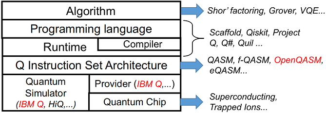
Figure 3: Overview of quantum computer system stack

There has been a lot of research on each layer of the quantum computer system stack shown in Fig. 3. The recent introduced cloud access to quantum devices such as the IBM Q  [21]  and Qiskit  [22] let users more easily write code and run experiments on the provided quantum devices and simulators based on (Open)QASM quantum circuit languages [8, 9].

The upper quantum algorithm can be described as a quantum-classical hybrid program containing a host program and multiple quantum kernels. The host program can be written in a classic programming language such as C++ or Python, and the quantum part is written in a high-level quantum programming languages such as Scaffold [2] or Project Q [3]. The compiler infrastructure consists of a conventional host compiler such as GCC and a quantum compiler such as ScaffCC [5]. The quantum compiler works on the quantum part and generates quantum circuit IR (intermediate representation) belonging to a QISA. (Open)QASMs [8, 9, 10] do not consider the low-level constraints to interface with the quantum processor. They all lack control micro-architecture that implements and executes such instructions on a real quantum processor. To bridge the gap between quantum software and hardware, a quantum control micro-architecture QuMA [12] and an executable QISA – eQASM[11] are proposed, but only validated on a 2-qubit superconducting quantum processor.

II-C Quantum Noise and the Decoherence Problem

Real quantum systems suffer from unwanted interactions with the outside world. These unwanted interactions show up as noise in quantum information processing (QIP) systems. For example, both the entanglement of the quantum system with the surrounding environment and quantum measurements will lead to the disappearance of quantum coherence, denoted as quantum decoherence. Decoherence invalidates the quantum superposition principle and thus turns quantum computers into (at best) classical computers, negating the potential power offered by the quantumness of the algorithms [15]. To date, for the promising superconducting qubits, the longest coherence time is still within 10$\sim$100 µs [17]; a typical gate time is 20ns for single-qubit gates and $\sim$ 40 ns for 2-qubit gates, the duration of a measurement is typically 300ns - 1µs [11]. Assume a single-qubit gate time is $\tau_{u}$, a two-qubit gate time is 2$\tau_{u}$, and a measurement time is $\tau_{m}$ = $m\tau_{u}$, where $m$ is 15$\sim$50.

Due to decoherence, the quantum program must complete execution quickly before the qubit state is decayed. The longer a quantum program runs and the more operations it performs, the more it is susceptible to noise. Therefore, it is necessary to shorten the duration of qubits in superposition in the program.

II-D Motivation Examples against Decoherence

We select OpenQASM to carry out the research in this paper since it is supported by IBM Q and can be generated by quantum compilers such as ScaffCC. Table I lists main quantum instructions in OpenQASM. The built-in universal gate basis is “CNOT+$U(2)$”. All the single qubit gates and two-qubit CNOT gate shown in Fig. 2 are built in.

TABLE I: Main quantum-related statements in OpenQASM language

Statement	Description
qreg name[size];	Declare a named register of qubits
gate name(params) qargs body	Declare a unitary gate
U($\gamma,\beta,\delta$) qubit$|$qreg;	Apply built-in single qubit gate(s)
CX qubit$|$qreg,qubit$|$qreg;	Apply built-in CNOT gate(s)
measure qubit$|$qreg -$>$ bit$|$creg;	Make measurement(s) in $Z$ basis
gatename(params) qargs;	Apply a user-defined unitary gate

II-D1 Lifetime of a qubit

⬇

1int i=0;

2i=i+1;

3int j=1;

4j+=i*2;

5return j;

(a)

⬇

1int i=0,j=1;

2i=i+1;

3j+=i*2;

4return j;

(b)

Figure 4: C program examples: different declaration locations for variable j

In the classical program such as C program shown in Fig. 4, moving int j=1 from line 3 of (a) to line 1 of (b) does not influence the execution result. However, as shown in Fig. 1 (a), qubits a[0] and a[1] are applied Hadamard operation at line 3, entering superposition state, and start their lifetime. The lifetime of a[1] ends after the measurement at line 6, occupying $(3+2m)\tau_{u}$. During the period, the measure at line 4 is independent of a[1], however, it makes the fragile qubit a[1] have to wait on the superposition before executing the CNOT and accumulate error, accordingly increasing the program’s error rate. If decomposing h a; and delaying h a[1]; at line 5 of Fig. 1 (b), the lifetime of a[1] will be reduced to $(3+m)\tau_{u}$. Section IV will show the movement improves the accuracy of the program running on a real IBM Q 5 Tenerife.

II-D2 Parallel Execution

In order to better use the fragile physical qubits, the parallelization of quantum circuits has been studied [18, 19]. The recent eQASM [11] adopts Single-Operation-Multiple-Qubit (SOMQ, similar to classical SIMD) execution, and a Very-Long-Instruction-Word (VLIW) architecture. The former supports applying a single quantum operation on multiple qubits, while the latter can combine multiple different quantum operations into a quantum bundle. These parallel features need be considered when converting quantum programs into physical quantum circuits. In this paper, we assume that neighboring gates operating on disjoint qubit subsets can always be applied in parallel, which is a common assumption for quantum technologies.

⬇

1qreg q[16];

2creg c[16];

3h q[1];

4h q[2];

5cx q[2], q[3];

6h q[2];

7h q[6];

8cx q[6], q[11];

9cx q[1], q[2];

10h q[11];

11h q[6];

12cx q[6], q[11];

13cx q[11], q[1];

14…

(a) Before

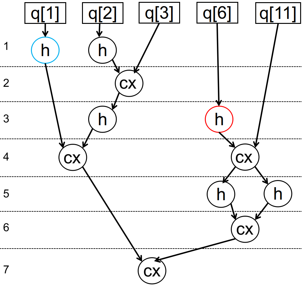
(b) Before: Layered bundle format

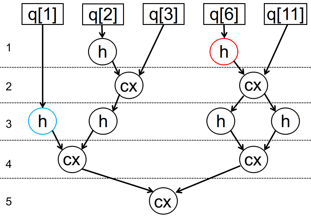
(c) After: Layered bundle format

⬇

1qreg q[16];

2creg c[16];

3h q[2];

4h q[6];

5cx q[2], q[3];

6cx q[6], q[11];

7h q[1];

8h q[2];

9h q[11];

10h q[6];

11cx q[1], q[2];

12cx q[6], q[11];

13cx q[11], q[1];

14…

(d) After

Figure 5: OpenQASM program example: package operations into layered bundles

Take the quantum program in Fig. 5 (a) as an example, this code fragment is part of a workload provided by ProjectQ[3], which is used to entangle a given number of qubits on IBM Q’s 16-qubit quantum computer. Due to the parallelism of the quantum hardware and architecture, we can analyze the dependencies of qubit operations in the program and package them into layered bundles, where operations on the same layer is a bundle and can be executed in parallel. Fig. 5 (b) shows the layered bundle format corresponding to code in Fig. 5 (a). The layered bundle format (defined in Section III-B) reflects the parallelism and execution dependencies among quantum operations. By further analysis, with the dependencies among quantum operations unchanged, the execution level of some quantum operations in Fig. 5 (b) can be adjusted to shorten the lifetime of the qubits involved, accordingly obtaining Fig. 5 (c). Thereinto, node ⓗ in column q[1] (h q[1];) is adjusted backward to layer 3, node ⓗ in column q[6] (h q[6];) is adjusted forward to layer 1, and the subsequent operations that depend on them are also adjusted. The depth of the adjusted layered bundle format is reduced from 7 to 5. According to Section II-C, a layer that only contains single qubit gates such as h costs $1\tau_{u}$, while the one contains two-qubit gates like cx costs $2\tau_{u}$. So the total execution time of the program will be shortened from $11\tau_{u}$ to $8\tau_{u}$ at maximum parallelization. Similarly, we can calculate the lifetime of qubits. After the transformation, the lifetime of q[1] reduces from $11\tau_{u}$ to $5\tau_{u}$. By topologically sorting the nodes in Fig. 5 (c), we can obtain the code sequence in Fig. 5 (d).

III Design

Following the idea of motivation examples described before, we have developed QLifeReducer to reduce the qubit lifetime in a quantum program, considering the parallelism of quantum operations. This section first gives an overview of the design then describes the related definitions and algorithms.

III-A Overview

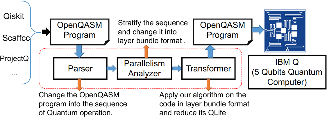
Figure 6: Overview of the QLifeReducer

The QLifeReducer copes with an input OpenQASM program, and outputs the optimized OpenQASM code with shortened qubit lifetime. The input program might come from ScaffCC[5], ProjectQ[3], QISKit[6] or other OpenQASM provider. As shown in Fig. 6, there are three core modules in the QLifeReducer. The Parser mainly performs macro expansion, that is, expanding user-defined gates (Table I), and obtains a sequence of built-in quantum instructions. The Parallelism Analyzer (described in Section III-C) then analyzes the expanded sequence and packages each sequence of parallelizable operations into a bundle, forming the layered bundle format discussed in Section II-D. After that, the Transformer (described in Section III-D) analyzes the layered bundle format and adjusts it to reduce the qubit lifetime, then converts the adjusted one to the corresponding OpenQASM code. The output OpenQASM program can be run on the quantum backend such as IBM Q quantum computer or simulator.

In the following subsections, we will use the example in Fig. 5 to explain main algorithms of the QLifeReducer.

III-B Definitions

Definition 1 ( Qubit Set of an Instruction).

For a quantum instruction $\iota$, the qubit set of $\iota$ is denoted as $S(\iota)$ that contains the qubits operated by $\iota$. For example, if $\iota$ is “CX q[1],q[2]”, then $S(\iota)$ = {q[1], q[2]}.

Definition 2 (Overlapped).

For two quantum instructions $\iota_{1}$ and $\iota_{2}$, if

$$S(\iota_{1})\cap S(\iota_{2})\neq\phi,$$

then they are overlapped with each other.

Overlapped instructions cannot be executed in parallel because only one quantum instruction can be applied on the intersecting qubit at the same time.

Definition 3 (Parallelizable).

For two quantum instructions $\iota_{1}$ and $\iota_{2}$, if

$$S(\iota_{1})\cap S(\iota_{2})=\phi,$$

then they are parallelizable with each other.

Parallelizable instructions can be executed in parallel.

Definition 4 (Bundle).

A bundle is a set of quantum instructions that are parallelizable with each other. All instructions in one bundle can be executed in parallel.

The qubit set of a bundle is the union set of the qubit set of all the instructions in the bundle. For a bundle $b$,

$$S(b)=\bigcup\limits_{\iota\in b}S(\iota)$$

Definition 5 (Layered bundle format).

The layered bundle format of a quantum program can be represented as a directed acyclic graph, in which all the qubits involved are start nodes at layer 0 and instruction operators in each bundle are nodes at the same layer like Fig. 5 (b). Each directed edge $<o,\iota>$ connects an instruction operator $\iota$ (arc head) and another instruction operator or a qubit $o$ (arc tail) which $\iota$ directly depends on, making instructions connected in execution order.

We denote the layer of an instruction $\iota$ as $L(\iota)$. If there is directed edge $<n_{2},n_{1}>$ in the layered bundle format, then node $n_{1}$ is the successor of node $n_{2}$, if further satisfying $L(n_{2})+1=L(n_{1})$, then $n_{1}$ is the next-layer successor of $n_{2}$.

III-C The Algorithm for Parallelism Analyzer

As shown in Fig. 6, the Parallelism Analyzer is responsible for converting the quantum code (Fig. 5 (a)) into the layered bundle format (Fig. 5 (b)), and the main algorithm is described in Alg. 1. First, an empty array of bundles $B$ is initialized, then it attempts to find a sequence of parallelizable instructions to form a bundle in each iteration of the outer while loop. During each iteration, it first creates an empty bundle $b$ as the current bundle and an empty set $Q$ saving qubits operated by any instruction in $b$, then determines whether each instruction $I[index]$ processed in turn can be executed in parallel with instructions in $b$ by deciding whether the qubit intersection $Q\cap S(I[index])$ is empty. If $I[index]$ can be parallel with $b$, it will be added into $b$, and the operated qubits will also be added into $Q$. If the instruction is overlapped with $b$, then $b$ is complete and can be added to $B$. The iteration is then over and the next instruction will be handled in the next iteration.

Algorithm 1 Transform code into layered bundle format

Array of quantum instructions: $I$

2:Array of bundles: $B$

function stratify(Instruction I[])

4:    $B\leftarrow an\ empty\ array\ of\ bundles$

    $index\leftarrow I.start$

6:    while $index\neq I.end$ do

        $b\leftarrow a\ new\ empty\ bundle$

8:        $Q\leftarrow\phi$

        while $Q\cap S(I[index])=\phi$ do

10:           $Q\leftarrow Q\cup S(I[index])$

           $b\leftarrow b\cup\{I[index]\}$

12:           $index\leftarrow index+1$

        end while

14:        $B.append(b)$

    end while

16:    return $B$

end function

The code in layered bundle format will help us identify the instructions that might be shifted. Furthermore, it is also a basis of parallelizing quantum instructions and mapping them into parallel quantum circuits in our future work.

III-D Algorithms for the Transformer

The Transformer performs two steps, first adjusts the layered bundle format to shorten the qubit lifetime, i.e.,from Fig. 5 (b) to (c); then converts the adjusted layered bundle format to OpenQASM code, i.e.,from (c) to (d). The first step is the core of the module and will be illustrated via Fig. 7 .

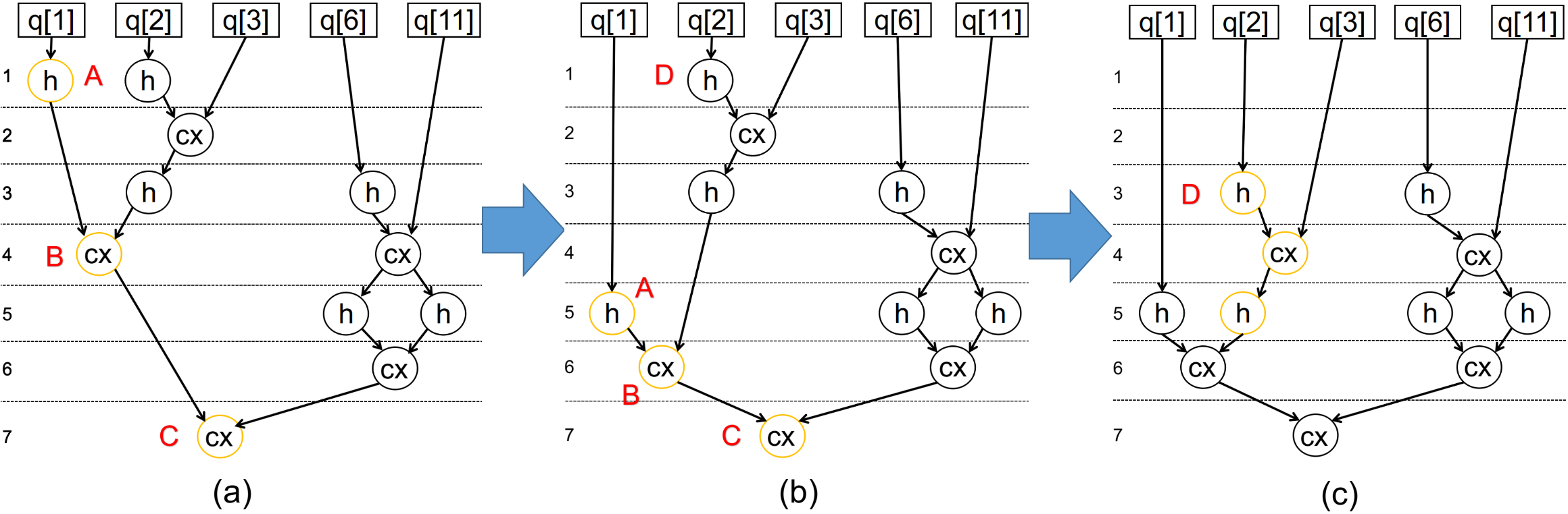
Figure 7: Transformation process to reduce the qubit lifetime

III-D1 Main Idea of the Adjustment

First, we need recognize instructions that should be adjusted. As discussed in Section II, an instruction $\iota$ starts the lifetime of a qubit $q$ only when it changes the qubit from ground state into superposition state. If the next instruction $\iota^{\prime}$ operating on $q$ is not the next-layer successor of $\iota$, $\iota$ could be delayed. In Fig. 7 (a), the h gate operating on q[1] at layer 1 (labelled A) starts the lifetime of q[1]. Since A’s successor (node B) is at layer 4, A could be delayed to shorten the lifetime of q[1].

Second, for an instruction $\iota$ to be delayed, we need decide at which layer $\iota$ could be put, and the adjustment must shorten the qubit lifetime without changing the execution order of instruction operators applied on a certain qubit. We need iteratively analyze each successor $\iota^{\prime}$ of $\iota$, and ensure that the adjusted layer of $\iota$, denoted as $L^{\prime}(\iota)$, is not less than the layer of other operand which $\iota^{\prime}$ depends on. Continue to consider Fig. 7 (a), B (the successor of A) has another operand q[2] at layer 3, so $L^{\prime}({\texttt{\small A}})\geq 3$ and $L^{\prime}({\texttt{\small A}})\leq L^{\prime}({\texttt{\small B}})-1$; we further analyze B and its successor C, and obtain $L^{\prime}({\texttt{\small B}})\geq 6$ and $L^{\prime}({\texttt{\small B}})\leq L^{\prime}({\texttt{\small C}})-1$ since C’s another operand is q[6] at layer 6. Because C has no successor, C should not be adjusted, i.e.,$L^{\prime}({\texttt{\small C}})=L({\texttt{\small C}})$. By solving the above constraints, we can get $L^{\prime}({\texttt{\small B}})=6,L^{\prime}({\texttt{\small A}})=5$ and the adjusted format is shown in Fig. 7 (b). Similarly, we can adjust D and get Fig. 7 (c).

Third, if the lowest layer that contains operators is layer $n$ ($n>1$), then the layer and its successors could move forward to ($n-1$) layers. For example, layer 3 is the lowest layer that contains operators, thus layers 3$\sim$7 could move forward to 1$\sim$5, accordingly transforming from Fig. 7 (c) to Fig. 5 (c).

III-D2 Data Structures

To implement the main idea, we design data structures for qubits and instructions (or called operation). A qubit is represented as a triple $q=({{\texttt{\small id}}},I,state)$, where

• id is the unique identifier of the qubit.

• $I$ is an ordered list of instructions operating on the qubit. The order of instructions in $I$ depends on their execution order in the original program.

• $state$ is the qubit state, whose value can be GROUND or NOTGROUND, representing ground state and superposition state, respectively.

An instruction in the layered bundle format is represented as $\iota=({\texttt{\small id}},op,seq,S,visited)$ contains four elements.

• id is the unique identifier of the instruction.

• $op$ is the operator of the instruction, e.g. h, cx, measure.

• $seq$ indicates the layer of the instruction, e.g. A$.seq=1$ in Fig. 7 (a).

• $S$ is the qubit set of the instruction.

• $visited$ is a bool flag indicating whether the instruction has been visited.

III-D3 The Main Algorithm of the Transformer

Alg. 2 gives the definition of function transform that adjusts the code to reduce the qubit lifetime. It traverses all instructions in each bundle. For an unvisited instruction $\iota$, if any of its operands is in GROUND state, that is, function $checkQ(\iota,{\texttt{\small NOTGROUND}})$ returns false, instruction $\iota$ could be delayed. Then function transform will call function adjust to adjust related instructions. Alg. 3 defines the auxiliary functions invoked by Alg. 2 .

Algorithm 2 Transform code to reduce the qubit lifetime

Array of bundles: $B$

2:Array of bundles with shorter qubit lifetime

function transform(Bundle B[])

4:    $index\leftarrow B.start$

    while $index\neq B.end$ do

6:        for all instruction $\iota\in B[index]$ do

           if $(checkQ(\iota,{\texttt{\scriptsize NOTGROUND}})=$ True) then

8:               continue

           end if

10:           if $\iota.visited=$ True then

               continue

12:           end if

           $\iota.visited\leftarrow$ True

14:           $setQ(\iota,{\texttt{\scriptsize NOTGROUND}})$

           adjust$(\iota,B)$

16:        end for

        $index\leftarrow index+1$

18:    end while

    $index\leftarrow B.start$ $\triangleright$ remove empty bundles at lower layers

20:    while $B[index]\ is\ empty$ do

        $index\leftarrow index+1$

22:    end while

    $B.start\leftarrow index$

24:    return $B$

end function

Algorithm 3 Set and Check Qubit State

function $setQ$(Instruction $\iota$, State state)

    for all $q\in S(\iota)$ do

        $q.state\leftarrow state$

    end for

end function

function $checkQ$(Instruction $\iota$, State state)

    for all $q\in S(\iota)$ do

        if $q.state\neq state$ then

           return False

        end if

    end for

    return True

end function

III-D4 Algorithm on Adjustment

Algorithm 4 Adjust an Instruction

function $adjust$(Instruction $\iota$, Bundle $B[]$)

2:    $Q\leftarrow S(\iota)$

    $cur\leftarrow\iota.seq+1$ $\triangleright$ $\iota\ belongs\ to\ B[\iota.seq]$

4:    $bstack\leftarrow initialize\ an\ empty\ bundle\ stack$

    $bstack.push(\{\iota\})$

6:    $flag\leftarrow$ False

    while $cur\neq B.end$ and $flag=$False do

8:        $b\leftarrow a\ new\ empty\ bundle$

        for all $\iota_{2}\in B[cur]$ do

10:           if $\iota_{2}.visited=$False and $S(\iota_{2})\cap Q\neq\phi$ then

               if $\iota_{2}.op={\texttt{\scriptsize measure}}$ then

12:                  $flag\leftarrow$ True

                  $setQ(\iota_{2},{\texttt{\scriptsize GROUND}})$

14:               end if

               $b\leftarrow b\cup\{\iota_{2}\}$

16:               $Q\leftarrow Q\cup S(\iota_{2})$

               $\iota_{2}.visited\leftarrow$ True

18:               $B[cur]\leftarrow B[cur]\setminus\{\iota_{2}\}$ $\triangleright$ remove $\iota_{2}$ from $B[cur]$

           end if

20:        end for

        if $b\ is\ not\ empty$ then

22:           $bstack.push(b)$

        end if

24:        $cur\leftarrow cur+1$

    end while

26:    $last\leftarrow bstack.top()$ $\triangleright$ The last instruction that enters the stack

    $line=last.seq$

28:    while $bstack\ is\ not\ empty$ do

        $b\leftarrow bstack.pop()$

30:        $B[line]\leftarrow B[line]\cup b$

        $line\leftarrow line-1$

32:    end while

end function

Alg. 4 shows the pesudo code of function adjust to do adjustment related to a given instruction $\iota$ in an array of bundles $B$. The adjustment should keep the original execution order of operations related to each qubit, and an instruction must not execute later than its successor. To adjust an instruction $\iota$, a bundle stack $bstack$ is introduced to save bundles of instructions to be adjusted, and it is initialized as a stack with only one element $\{\iota\}$. A qubit set $Q$ is introduced to collect all qubits depended by instructions saved in $bstack$, and is initialized as $S(\iota)$. Function adjust traverses and copes with all the successors of $\iota$ until reaching the end of the program or a measure operation to any qubit in $Q$. When the function finds an instruction $\iota_{2}$ that is overlapped with $Q$, it means that $\iota_{2}$ is the successor of some instructions in $bstack$ and we need delay them together to keep the order constraints. So $\iota_{2}$ would be pushed into $bstack$ and $S(\iota_{2})$ also be merged into $Q$. After the function finds all the instructions that need to be postponed, it will pop the stack and decide the new layer of each instruction according to the last one’s layer.

The $transform$ algorithm won’t increase the number of bundles. From Alg. 4 you can see, what we adjust on the quantum circuit program includes: 1) Remove an instruction $\iota_{2}$ from a bundle in the original quantum circuit, and add $\iota_{2}$ into a temporary bundle $b$; 2) The formed temporary bundle is pushed into $bstack$, and will be popped to adjust its layer later.

III-E Algorithm Complexity

Suppose a quantum circuit program has $n$ quantum instructions applied on $d$ qubits, $adjust(\iota,B)$ handles each unvisited instruction in $B[cur]$ ( $cur>L(\iota)$ ), thus the time complexity of Alg. 4 is $O(n)$. For function $transform(B)$, it invokes $adjust()$ less than $d$ times, so the time complexity of Alg. 2 is $O(dn)$.

IV Evaluation

This section first introduces the QLifeReducer prototype implementing algorithms mentioned in Section III, then evaluates the effect of QLifeReducer on quantum program transformation, including accuracy and efficiency.

IV-A Prototype

We have built QLifeReducer and a simulator for evaluation on Linux with C++. As shown in Fig. 6, QLifeReducer takes the text of an OpenQASM program as input and outputs the transformed OpenQASM program. First the Parser, where classes Instruction and Qubit are defined, analyzes the input text and builds the corresponding Instruction list and Qubit list. Then the Parallelism Analyzer, where class Bundle is defined, analyzes the lists of Instruction and Qubit, and builds the array of Bundle according to Alg. 1. Finally, the Transformer analyzes the lists of Instruction and Qubit as well as the array of Bundle, and outputs the transformed code according to Alg. 2 and 4. The total number of LOC (lines of code) in QLifeReducer is 1106.

Since the availability of the real quantum computer is extremely limited, we build a simulator that calculates the lifetime of each qubit and the execution time about the input OpenQASM program in the way discussed in Section II-D2. The number of LOC in the simulator is 424.

IV-B Methodology

IV-B1 Accuracy

There is no available quantum simulator considering quantum noise and the accuracy of programs when running on the simulators is always 100%. So we use the real quantum device, IBM Q 5 Tenerife, to evaluate the accuracy of two quantum circuits before and after transformation in Fig. 8. We discuss the detail in Section IV-C.

IV-B2 Qubit Lifetime

The quantum hardware has some limitations. It has serious error rate on quantum gates and measurements, and only supports 5 qubits at most which is not enough for many quantum programs. Although the simulator cannot simulate quantum noise, it can calculate the execution time and the qubit lifetime of the program. Due to decoherence, these features would also affect the accuracy of quantum circuits. So we use our quantum simulator to evaluate the execution time, the longest qubit lifetime and average qubit lifetime of quantum programs.

TABLE II: Quantum workloads

Program	Description	Qubits
3G	3-qubit Grover’s algorithm	3
DE	Deutsch’s algorithm that exponentially accelerates classical algorithms	2
4QFT, 5QFT	Quantum Fourier Transform using 4 or 5 qubits	4,5
IBM 6	Entangle 6 qubits in IBM’s quantum chip and test their accuracy	16
NIQFT	Inverse Quantum Fourier Transform using N qubits, where N could be 4, 8, 16, 32, 64	N

Table II lists the tested quantum workloads, where 3G, DE, 4QFT and 5QFT come from Qiskit, IBM 6 from Project Q. Qiskit also provides 4IQFT, and we expand it with more qubits, i.e.,obtaining NIQFT.

IV-C Experiments on Quantum Hardware

IBM Q has provided several superconducting quantum computers: IBM Q 20 Tokyo, IBM Q 14 Melbourne, IBM Q 5 Tenerife and IBM Q 5 Yorktown. Only Tenerife and Yorktown can be used for public, but Yorktown is under maintenance. So we choose Tenerife for our experiments. Table III lists error rate and other parameters for each quibit in Tenerife.

TABLE III: Parameters of IBM Q 5-qubit Tenerife

	$Q_{0}$	$Q_{1}$	$Q_{2}$	$Q_{3}$	$Q_{4}$
Frequency(GHz)	5.25	5.30	5.35	5.43	5.18
Single-qubit gate error$(10^{-3})$	0.69	1.29	1.12	1.97	1.80
Readout error($10^{-2}$)	6.10	6.90	7.90	7.80	25.20
Multi-qubit Gate error		CX10	CX20	CX32	CX42
($10^{-2}$)		3.22	2.59	7.46	5.53
			CX21	CX34
			4.23	6.73

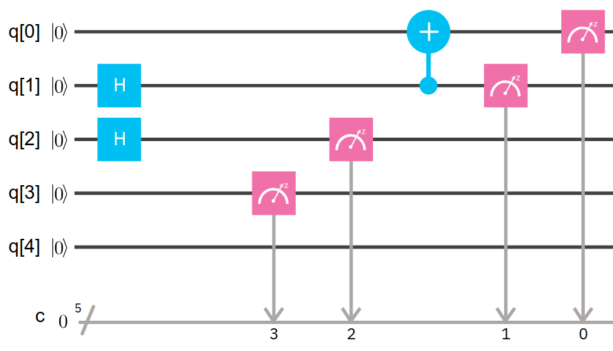
(a) Before transformation

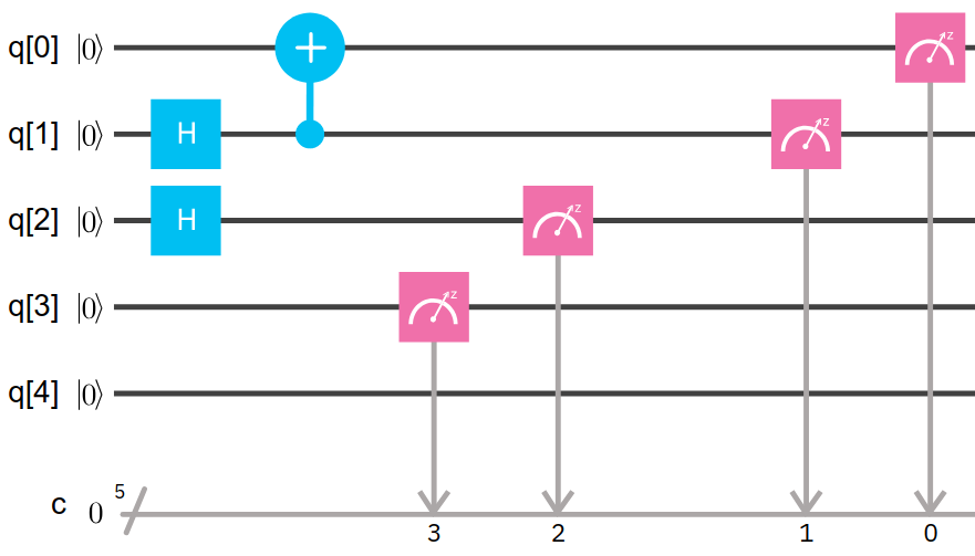
(b) After transformation

State	Before	After
00	46.59%	46.01%
01	7.80%	7.52%
10	6.44%	5.12%
11	39.18%	41.35%
Error (01,10)	14.24%	12.64%

(c) Comparison between two circuits

Figure 8: Quantum circuits testing on IBM Q 5 Tenerife

We use the accuracy of quantum circuits of Bell State[20] to show the benefits of QLifeReducer. Fig. 8 (a) and (b) show the quantum circuits before and after transformation by QLifeReducer, and both of them will bound qubits q[0] and q[1] into Bell State. In the circuits, we focus on the result of qubits q[0] and q[1] and ignore the result of q[2] and q[3]. The only difference between the two circuits is the time gap between the H gate on q[1] and CNOT on q[0], q[1] which are used to create a Bell State. After the CNOT operation, q[0] and q[1] are in Bell State and their state is $\frac{|00\rangle+|11\rangle}{\sqrt{2}}$. In an ideal quantum computer, the measured result of q[0] and q[1] should be 00 or 11 with both 50% probability. However, because of hardware error caused by the decoherence and quantum noise, there will be an amount of result 01 and 10 which are considered as error states. To reduce the effect of outliers, we run each circuit 1024 times in one group on Tenerife, and record the ratio of state $\ket{00},\ket{01},\ket{10}$ and $\ket{11}$. 25 groups for each circuit are tested on Tenerife, and the average ratios of each resulting state are listed on Fig. 8 (c). We see that the error rate (ratio of error states) reduces from 14.24% down to 12.64%. From the experimental results, we see that IBM’s quantum chips have significant noise, where the final error rate is higher than 10%. QLifeReducer indeed improves the accuracy of quantum circuits against decoherence for quantum computers with noise.

IV-D Evaluation on the Simulator

We run workloads listed in Table II on the self-developed simulator and Table IV lists the result.

TABLE IV: Test result of workloads obtained from the simulator

Workload	Execution time		Longest lifetime		Average lifetime
	before	after	before	after	before	after
3G	128	128	128	128	128	127
DE	20	20	20	19	4.8	4.6
4QFT	103	98	103	92	91.8	83.4
5QFT	126	126	126	126	126	104.4
IBM 6	306	246	300	246	211	162
4IQFT	68	68	68	34	42	29
8IQFT	150	150	150	38	80	32
16IQFT	362	362	362	46	172	37
32IQFT	978	978	978	62	420	46
64IQFT	2978	2978	2978	94	1172	62

The unit of values in Columns $2\sim 7$ is $\tau_{u}$, i.e.,the executiontime of single qubit gate, generally 20ns.

We see that QLifeReducer reduce the average qubit lifetime for every workload, and sometimes can reduce the total execution time of the program. The reduction is tiny when qubits number is less than 4(3G and DE). But as the number of qubits used in the program increases(other algorithms), the reduction of average qubit lifetime brought by QLifeReducer is prominent. The reason is that there is spatial locality in quantum program. Programmers tend to use several certain qubits in one part and QLifeReducer can reassemble the program and remove the spatial locality. This will help increase the program’s parallelism and also reduce the qubit lifetime. With the reduction of qubit lifetime, quantum system can further effectively control the use of qubits.

V Conclusion and Future Work

In this paper, we proposed QLifeReducer that can reduce the qubit lifetime of quantum programs considering the parallel execution of quantum circuits. With a parallelism analyzer, QLifeReducer converts the quantum program into layered bundle format. Then QLifeReducer applies transformation algorithm on the code in layered bundle format and reduces its qubit lifetime and execution time. By shortening the qubit lifetime of the quantum program, QLifeReducer can reduce the error rate caused by decoherence of qubits which is unavoidable in the NISQ quantum computers.

Our future work will include the efficiency improvement of the transformation algorithms and the combination with other optimization methods. We are also intend to build a more comprehensive quantum simulator for evaluation that considers the noise in quantum hardware.

References

- [1] IBM, “Ibm makes quantum computing available on IBM Cloud to accelerate innovation,” https://www-03.ibm.com/press/us/en/pressrelease/49661.wss, 4 May 2016.
- [2] A. J. Abhari, A. Faruque, M. J. Dousti et al., “Scaffold: Quantum programming language,” Princeton University, Tech. Rep. TR-934-12, 2012.
- [3] D. S. Steiger, T. Häner, and M. Troyer, “ProjectQ: an open source software framework for quantum computing,” Quantum, vol. 2, p. 49, Jan. 2018. [Online]. Available: https://doi.org/10.22331/q-2018-01-31-49
- [4] K. M. Svore, A. Geller, M. Troyer et al., “Q#: Enabling scalable quantum computing and development with a high-level domain-specific language,” in RWDSL 2018. ACM, February 2018. [Online]. Available: https://dl.acm.org/citation.cfm?id=3183901
- [5] A. J. Abhari, S. Patil, D. Kudrow, J. Heckey, A. Lvov, F. T. Chong, and M. Martonosi, “ScaffCC: A framework for compilation and analysis of quantum computing programs,” in 11th CF. New York, NY, USA: ACM, 2014, pp. 1:1–1:10. [Online]. Available: http://doi.acm.org/10.1145/2597917.2597939
- [6] A. Cross, “The IBM Q experience and QISKit open-source quantum computing software,” Bulletin of the American Physical Society, 2018.
- [7] T. Häner, D. S. Steiger, K. Svore, and M. Troyer, “A software methodology for compiling quantum programs,” Quantum Science and Technology, vol. 3, no. 2, p. 020501, 2018. [Online]. Available: https://arxiv.org/pdf/1604.01401.pdf
- [8] K. M. Svore, A. V. Aho, A. W. Cross, I. Chuang, and I. L. Markov, “A layered software architecture for quantum computing design tools,” IEEE Computer, vol. 39, no. 1, pp. 74–83, 2006. [Online]. Available: doi.ieeecomputersociety.org/10.1109/MC.2006.4
- [9] A. W. Cross, L. S. Bishop, J. A. Smolin, and J. M. Gambetta, “Open quantum assembly language,” arXiv:1707.03429, 2017.
- [10] R. S. Smith, M. J. Curtis, and W. J. Zeng, “A practical quantum instruction set architecture,” ArXiv e-prints, Feb. 2017.
- [11] X. Fu, L. Riesebos, M. A. Rol et al., “eQASM: An executable quantum instruction set architecture,” in HPCA 2019, Feb 2019, pp. 224–237.
- [12] X. Fu, M. A. Rol, C. C. Bultink et al., “A microarchitecture for a superconducting quantum processor,” IEEE Micro, vol. 38, no. 3, pp. 40–47, May 2018.
- [13] J. Preskill, “Quantum computing in the NISQ era and beyond,” ArXiv e-prints, Jan. 2018.
- [14] D. Gottesman, “An introduction to quantum error correction and fault-tolerant quantum computation,” in Proc. of Symposia in Applied Matthematics, 2010. [Online]. Available: http://arxiv.org/abs/0904.2557
- [15] W. H. Zurek, “Decoherence and the transition from quantum to classical,” Physics Today, vol. 44, pp. 36–44, Oct. 1991. [Online]. Available: https://physicstoday.scitation.org/doi/10.1063/1.881293
- [16] T. S. Metodi, A. I. Faruque, and F. T. Chong, Quantum Computing for Computer Architects, Second ed., ser. Synthesis Lectures on Computer Architecture #13. USA: Morgan & Claypool Publishers, Mar. 2011.
- [17] M. Reagor, W. Pfaff, C. Axline et al., “Quantum memory with millisecond coherence in circuit qed,” Phys. Rev. B, vol. 94, p. 014506, Jul 2016. [Online]. Available: https://link.aps.org/doi/10.1103/PhysRevB.94.014506
- [18] A. Broadbent and E. Kashefi, “Parallelizing quantum circuits,” Theoretical Computer Science, vol. 410, no. 26, pp. 2489 – 2510, 2009. [Online]. Available: http://www.sciencedirect.com/science/article/pii/S0304397508009377
- [19] O. D. Matteo and M. Mosca, “Parallelizing quantum circuit synthesis,” Quantum Science and Technology, vol. 1, no. 1, p. 015003, 2016. [Online]. Available: http://stacks.iop.org/2058-9565/1/i=1/a=015003
- [20] M. A. Nielsen and I. L. Chuang, Quantum Computation and Quantum Information, 10th Anniversary ed. UK: Cambridge University Press, 2010.
- [21] S. J. Devitt., “Performing quantum computing experiments in the cloud,” vol. 94, 2016.
- [22] D. Lubensky, “Quantum computing gets an API and SDK,” https://developer.ibm.com/dwblog/2017/quantum-computing-api-sdk-david-lubensky/, 6 Mar. 2017.