Automatic Target Detection for Sparse Hyperspectral Images

Abstract

In this work, a novel target detector for hyperspectral imagery is developed. The detector is independent on the unknown covariance matrix, behaves well in large dimensions, distributional free, invariant to atmospheric effects, and does not require a background dictionary to be constructed. Based on a modification of the robust principal component analysis (RPCA), a given hyperspectral image (HSI) is regarded as being made up of the sum of a low-rank background HSI and a sparse target HSI that contains the targets based on a pre-learned target dictionary specified by the user. The sparse component is directly used for the detection, that is, the targets are simply detected at the non-zero entries of the sparse target HSI. Hence, a novel target detector is developed, which is simply a sparse HSI generated automatically from the original HSI, but containing only the targets with the background is suppressed. The detector is evaluated on real experiments, and the results of which demonstrate its effectiveness for hyperspectral target detection especially when the targets are well matched to the surroundings.

1 Introduction

1.1 What Is a Hyperspectral Image?

An airborne hyperspectral imaging sensor is capable of simultaneously acquiring the same spatial scene in a contiguous and multiple narrow (0.01 - 0.02 $\upmu$m) spectral wavelength (color) bands Shaw02 ; manolakis2003hyperspectral ; manolakis_lockwood_cooley_2016 ; 974715 ; 7564440 ; ZHANG20153102 ; 6555921 ; PLAZA2009S110 ; 6509473 ; bookJocekynToaPPEAR ; DallaMura2011 ; prasad2011optical ; chanussotDec2009 . When all the spectral bands are stacked together, the result is a hyperspectral image (HSI) whose cross-section is a function of the spatial coordinates and its depth is a function of wavelength. Hence, an HSI is a 3-D data cube having two spatial dimensions and one spectral dimension. Thanks to the narrow acquisition, the HSI could have hundreds to thousands of contiguous spectral bands. Having this very high level of spectral detail gives better capability to see the unseen.

Each band of the HSI corresponds to an image of the surface covered by the field of view of the hyperspectral sensor, whereas each pixel in the HSI is a $p$-dimensional vector, $\mathbf{x}\in\mathbb{R}^{p}$ ($p$ stands for the total number of spectral bands), consisting of a spectrum characterizing the materials within the pixel. The spectral signature of $\mathbf{x}$ (also known as reflectance spectrum) shows the fraction of incident energy, typically sunlight, that is reflected by a material from the surface of interest as a function of the wavelength of the energy manolakis2003hyperspectral ; JoanaThesis .

The HSI usually contains both pure and mixed pixels manolakis2003hyperspectral ; Manolakis09 ; 6048900 ; 6504505 ; 5658102 ; 6351978 . A pure pixel contains only one single material, whereas a mixed pixel contains multiple materials, with its spectral signature representing the aggregate of all the materials in the corresponding spatial location. The latter situation often arises because hyperspectral images are collected hundreds to thousands of meters away from an object so that the object becomes smaller than the size of a pixel. Other scenarios might involve, for example, a military target hidden under foliage or covered with camouflage material.

1.2 Hyperspectral Target Detection: Concept and Challenges

With the rich information afforded by the high spectral dimensionality, hyperspectral imagery has found many applications in various fields, such as astronomy, agriculture Patel2001 ; Datt2003 , mineralogy Lehmann2001 , military manolakis2002detection ; Stein02 ; 4939406 , and in particular, target detection Shaw02 ; manolakis2003hyperspectral ; Manolakis14 ; Manolakis09 ; manolakis2002detection ; 7739987 ; 7165577 ; 8069001 ; Frontera14 ; 6378408 . Usually, the detection is built using a binary hypothesis test that chooses between the following competing null and alternative hypothesis: target absent ($H_{0}$), that is, the test pixel $\mathbf{x}$ consists only of background, and target present ($H_{1}$), where $\mathbf{x}$ may be either fully or partially occupied by the target material.

It is well known that the signal model for hyperspectral test pixels is fundamentally different from the additive model used in radar and communications applications manolakis_lockwood_cooley_2016 ; Manolakis09 . We can regard each test pixel $\mathbf{x}$ as being made up of $\mathbf{x}=\alpha\,\mathbf{t}$ + $(1-\alpha)\,\mathbf{b}$, where $0\leq\alpha\leq 1$ designates the target fill-fraction, $\mathbf{t}$ is the spectrum of the target, and $\mathbf{b}$ is the spectrum of the background. This model is known as replacement signal model, and hence, when a target is present in a given HSI, it replaces (that is, removes) an equal part of the background manolakis_lockwood_cooley_2016 . For notational convenience, sensor noise has been incorporated into the target and background spectra (i.e., the vectors $\mathbf{t}$ and $\mathbf{b}$ include noise) manolakis_lockwood_cooley_2016 .

In particular, when $\alpha=0$, the pixel $\mathbf{x}$ is fully occupied by the background material (target not present). When $\alpha=1$, the pixel $\mathbf{x}$ is fully occupied by the target material and is usually referred to as the full or resolved target pixel. Whereas when $0<\alpha<1$, the pixel $\mathbf{x}$ is partially occupied by the target material and is usually referred to as the subpixel or unresolved target Manolakis09 .

A prior target information can often be provided to the user. In real-world hyperspectral imagery, this prior information may not be only related to its spatial properties (e.g., size, shape, texture) and which is usually not at our disposal, but to its spectral signature. The latter usually hinges on the nature of the given HSI where the spectra of the targets of interest have been already measured by some laboratories or with some handheld spectrometers.

Different Gaussian-based target detectors (e.g., Matched Filter Manolakis00 ; Nasrabadi08 , Normalized Matched Filter kraut1999cfar , and Kelly detector Kelly86 ) have been developed. In these classical detectors, the target of interest to detect is known (e.g., its spectral signature is fully provided to the user).

However, the aforementioned detectors present several limitations in real-world hyperspectral imagery. The task of understanding and solving these limitations presents significant challenges for hyperspectral target detection.

• Challenge one: One of the major drawbacks of the aforementioned classical target detectors is that they depend on the unknown covariance matrix (of the background surrounding the test pixel) whose entries have to be carefully estimated, especially in large dimensions LEDOIT2004365 ; LedoitHoney ; AhmadCamsap2017 , and to ensure success under different environments JoanaThesis ; 7165577 ; 5606730 ; 6884641 ; 6894189 . However, estimating large covariance matrices has been a longstanding important problem in many applications and has attracted increased attention over several decades. When the spectral dimension is considered large compared to the sample size (which is the usual case), the traditional covariance estimators are estimated with a lot of errors unless some covariance regularization methods are considered LEDOIT2004365 ; LedoitHoney ; AhmadCamsap2017 . It implies that the largest or smallest estimated coefficients in the matrix tend to take on extreme values not because this is “the truth”, but because they contain an extreme amount of error LEDOIT2004365 ; LedoitHoney . This is one of the main reasons why the classical target detectors usually behave poorly in detecting the targets of interest in a given HSI.
  In addition, there is always an explicit assumption (specifically, Gaussian) on the statistical distribution characteristics of the observed data. For instance, most materials are treated as Lambertian because their bidirectional reflectance distribution function characterizations are usually not available, but the actual reflection is likely to have both a diffuse component and a specular component. This latter component would result in gross corruption of the data. In addition, spectra from multiple materials are usually assumed to interact according to a linear mixing model; nonlinear mixing effects are not represented and will contribute to another source of noise.
  

• Challenge two: The classical target detectors that depend on the target to detect $\mathbf{t}$ use only a single reference spectrum for the target of interest. This may be inadequate since in real-world hyperspectral imagery, various effects that produce variability to the material spectra (e.g., atmospheric conditions, sensor noise, material composition, and scene geometry) are inevitable 803418 ; 1000320 . For instance, target signatures are typically measured in laboratories or in the field with handheld spectrometers that are at most a few inches from the target surface. Hyperspectral images, however, are collected at huge distances away from the target and have significant atmospheric effects present.

Recent years have witnessed a growing interest in the notion of sparsity as a way to model signals. The basic assumption of this model is that natural signals can be represented as a “sparse” linear combination of atom signals taken from a dictionary. In this regard, two main issues need to be addressed: (1) how to represent a signal in the sparsest way, for a given dictionary? and (2) how to construct an accurate dictionary in order to successfully represent the signal?

Recently, a signal classification technique via sparse representation was developed for the application of face recognition 4483511 . It is observed that aligned faces of the same object with varying lighting conditions approximately lie in a low-dimensional subspace 1177153 . Hence, a test face image can be sparsely represented by atom signals from all classes. This representation approach has also been exploited in several other signal classification problems such as iris recognition 5339067 , tumor classification 1177153asf , and hyperspectral imagery unmixing 6555921 ; doi818245 ; 6200362 .

In this context, Chen et al. Chen11 have been inspired by the work in 4483511 , and developed an approach for sparse representation of hyperspectral test pixels. In particular, each test pixel $\mathbf{x}\in\mathbb{R}^{p}$ (either target or background) in a given HSI, is assumed to lie in a low-dimensional subspace of the $p$-dimensional spectral-measurement space. Hence, it can be represented by a very few atom signals taken from the dictionaries, and the recovered sparse representation can be used directly for the detection. For example, if a test pixel $\mathbf{x}$ contains the target (that is, $\mathbf{x}=\alpha\,\mathbf{t}+(1-\alpha)\,\mathbf{b}$, with $0<\alpha\leq 1$), it can be sparsely represented by atom signals taken from the target dictionary (denoted as $\mathbf{A}_{t})$; whereas, if $\mathbf{x}$ is only a background pixel (e.g., $\alpha=0$), it can be sparsely represented by atom signals taken from the background dictionary (denoted as $\mathbf{A}_{b}$). Very recently, Zhang et al. Zhang15 have extended the work done by Chen et al. in Chen11 by combining the idea of binary hypothesis and sparse representation together, obtaining a more complete and realistic sparsity model than in Chen11 . More precisely, Zhang et al. Zhang15 have assumed that if the test pixel $\mathbf{x}$ belongs to hypothesis $H_{0}$ (target absent), it will be modeled by the $\mathbf{A}_{b}$ only; otherwise, it will be modeled by the union of $\mathbf{A}_{b}$ and $\mathbf{A}_{t}$. This in fact yields a competition between the two hypotheses corresponding to the different pixel class label.

These sparse representation methods Chen11 ; Zhang15 are independent on the unknown covariance matrix, behave well in large dimensions, distributional free, and invariant to atmospheric effects. More precisely, they can alleviate the spectral variability caused by atmospheric effects, and can also better deal with a greater range of noise phenomena.

• Challenge three: The main drawback of these sparse representation methods Chen11 ; Zhang15 is the lack of a sufficiently universal dictionary, especially for the background $\mathbf{A}_{b}$; some form of in-scene adaptation would be desirable. The background dictionary $\mathbf{A}_{b}$ is usually constructed using an adaptive scheme (a local method) which is based on a dual concentric window centered on the test pixel, with an inner window region (IWR) centered within an outer window region (OWR), and only the pixels in the OWR will constitute the samples for $\mathbf{A}_{b}$. Clearly, the dimension of IWR is very important and has a strong impact on the target detection performance since it aims to enclose the targets of interest to be detected. It should be set larger than or equal to the size of all the desired targets of interest in the corresponding HSI, so as to exclude the target pixels from erroneously appearing in $\mathbf{A}_{b}$. However, information about the target size in the image is usually not at our disposal. It is also very unwieldy to set this size parameter when the target could be of irregular shape (e.g., searching for lost plane parts of a missing aircraft). Another tricky situation is when there are multiple targets in close proximity in the image (e.g., military vehicles in long convoy formation). Hence, the construction of $\mathbf{A}_{b}$ for the sparse representation methods is a very challenging problem since a contamination of it by the target pixels can potentially affect the target detection performance.

1.3 Goals and Outline

In this work, we handle all the aforementioned challenges by making very little specific assumptions about the background or target 8462257 ; 8677268 . Based on a modification of the recently developed robust principal component analysis (RPCA) Candes11 , our method decomposes an input HSI into a background HSI (denoted by $\mathbf{L}$) and a sparse target HSI (denoted by $\mathbf{E}$) that contains the targets of interest.

While we do not need to make assumptions about the size, shape, or number of the targets, our method is subject to certain generic constraints that make less specific assumption on the background or the target. These constraints are similar to those used in RPCA Candes11 ; NIPS2009_3704 , including

1. The background is not too heavily cluttered with many different materials with multiple spectra, so that the background signals should span a low-dimensional subspace, a property that can be expressed as the low-rank condition of a suitably formulated matrix ChenYu ; Zhang15b ; 7322257 ; 8260545 ; 8126244 ; Ahmad2017a ; 7312998 ;

2. The total image area of all the target(s) should be small relative to the whole image (i.e., spatially sparse), e.g., several hundred pixels in a million-pixel image, though there is no restriction on the target shape or the proximity between the targets.

Our method also assumes that the target spectra are available to the user and that the atmospheric influence can be accounted for by the target dictionary $\mathbf{A}_{t}$. This pre-learned target dictionary $\mathbf{A}_{t}$ is used to cast the general RPCA into a more specific form, specifically, we further factorize the sparse component $\mathbf{E}$ from RPCA into the product of $\mathbf{A}_{t}$ and a sparse activation matrix $\mathbf{C}$ 8462257 . This modification is essential to disambiguate the true targets from the background.

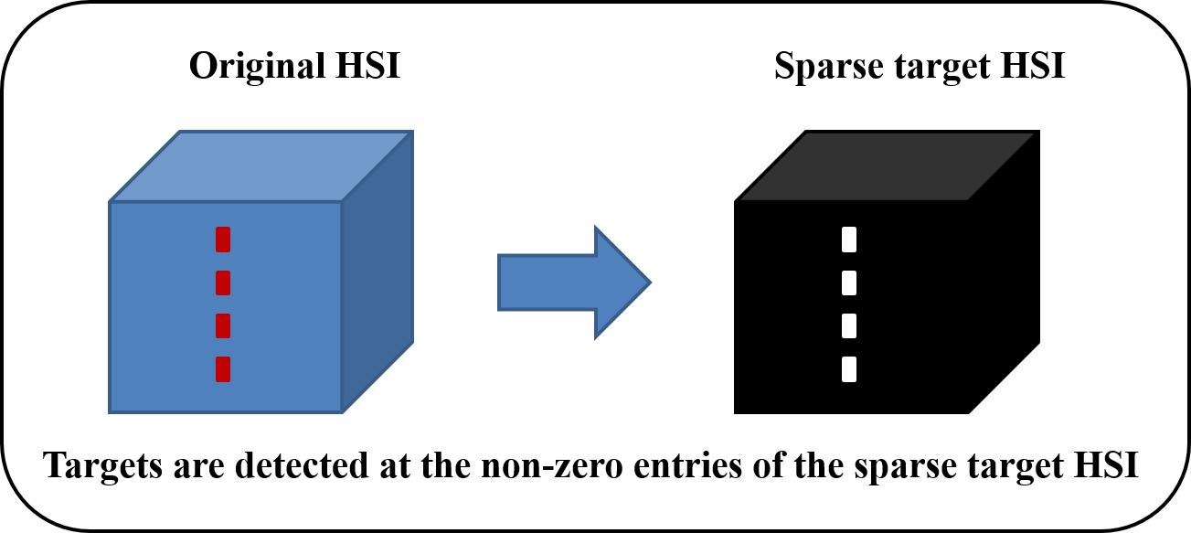
Figure 1: Sparse target HSI: our novel target detector.

After decomposing a given HSI into the sum of a low-rank HSI and a sparse HSI, the latter will define our detector. That is, the targets are detected at the non-zero entries of the sparse HSI. Hence, a novel target detector is developed, which is simply a sparse HSI generated automatically from the original HSI, but containing only the targets with the background is suppressed (see Fig. 1).

• The main advantages of our proposed detector are the following: (1) independent on the unknown covariance matrix; (2) behaves well in large dimensions; (3) distributional free; (4) invariant to atmospheric effects via the use of the target dictionary $\mathbf{A}_{t}$; and (5) does not require a background dictionary to be constructed.

This chapter is structured along the following lines. First comes an overview of some related works in Sect. 2. In Sect. 3, the proposed decomposition model as well as our novel target detector are briefly outlined. Section 4 presents real experiments to gauge the effectiveness of the proposed detector for hyperspectral target detection. The chapter ends with a summary of the work and some directions for future work.

1.4 Summary of Main Notations

Throughout this chapter, we depict vectors in lowercase boldface letters and matrices in uppercase boldface letters. The notation $(.)^{T}$ and $\mathrm{Tr}(.)$ stand for the transpose and trace of a matrix, respectively. In addition, $\mathrm{rank}(.)$ is for the rank of a matrix. A variety of norms on matrices will be used. For instance, $\mathbf{M}$ is a matrix, and $[\mathbf{M}]_{:,j}$ is the $j$th column. The matrix $l_{2,0}$, $l_{2,1}$ norms are defined by $\left\|\mathbf{M}\right\|_{2,0}=\#\left\{j\,:\,\left\|\left[\mathbf{M}\right]_{:,j}\right\|_{2}\,\not=\,0\right\}$, and $\left\|\mathbf{M}\right\|_{2,1}=\sum_{j}\left\|\left[\mathbf{M}\right]_{:,j}\right\|_{2}$, respectively. The Frobenius norm and the nuclear norm (the sum of singular values of a matrix) are denoted by $\left\|\mathbf{M}\right\|_{F}$ and $\left\|\mathbf{M}\right\|_{*}=\operatorname{Tr}\left(\mathbf{M}^{T}\,\mathbf{M}\right)^{(1/2)}$, respectively.

2 Related Works

Whatever the real application may be, somehow the general RPCA model needs to be subject to further assumptions for successfully distinguishing the true targets from the background. Besides the generic RPCA and our suggested modification discussed in Sect. 1.3, there have been other modifications of RPCA. For example, the generalized model of RPCA, named the low-rank representation (LRR) 6180173 , allows the use of a subspace basis as a dictionary or just uses self-representation to obtain the LRR. The major drawback in LRR is that the incorporated dictionary has to be constructed from the background and to be pure from the target samples. This challenge is similar to the aforementioned background dictionary $\mathbf{A}_{b}$ construction problem. If we use the self-representation form of LRR, the presence of a target in the input image may only bring about a small increase in rank and thus be retained in the background 8677268 .

In the earliest models using a low-rank matrix to represent the background Candes11 ; NIPS2009_3704 ; SPCPCandes , no prior knowledge on the target was considered. In some applications such as Speech enhancement and hyperspectral imagery, we may expect some prior information about the target of interest and which can be provided to the user. Incorporating this information about the target into the separation scheme in the general RPCA model should allow us to potentially improve the target extraction performance. For example, Chen and Ellis 6701883 , and Sun and Qin 7740039 , proposed a Speech enhancement system by exploiting the knowledge about the likely form of the targeted speech. This was accomplished by factorizing the sparse component from RPCA into the product of a dictionary of target speech templates and a sparse activation matrix. The proposed methods in 6701883 and 7740039 typically differ on how the fixed target dictionary of speech spectral templates is constructed. Our proposed model in Sect. 3 is very related to 6701883 and 7740039 . In real-world hyperspectral imagery, the prior target information may not be only related to its spatial properties (e.g., size, shape, and texture) and which is usually not at our disposal, but to its spectral signature. The latter usually hinges on the nature of the given HSI where the spectra of the targets of interest present have been already measured by some laboratories or with some handheld spectrometers.

3 Main Contribution

Suppose an HSI of size $h\times w\times p$, where $h$ and $w$ are the height and width of the image scene, respectively, and $p$ is the number of spectral bands. Our proposed modification of RPCA is mainly based on the following steps:

1. Let us consider that the given HSI contains $q$ pixels $\{\mathbf{x}_{i}\}_{i\in[1,\,q]}$ of the form:

   $$\mathbf{x}_{i}=\alpha_{i}\,\mathbf{t}_{i}+(1-\alpha_{i})\,\mathbf{b}_{i},~{}~{}~{}~{}0<\alpha_{i}\leq 1\,,$$

   where $\mathbf{t}_{i}$ represents the known target that replaces a fraction $\alpha_{i}$ of the background $\mathbf{b}_{i}$ (i.e., at the same spatial location). The remaining ($e-q$) pixels in the given HSI, with $e=h\times w$, are thus only background ($\alpha=0$).

2. We assume that all $\{\mathbf{t}_{i}\}_{i\in[1,\,q]}$ consist of similar materials, and thus they should be represented by a linear combination of $N_{t}$ common target samples $\{\mathbf{a}^{t}_{j}\}_{j\in[1,\,N_{t}]}$, where $\mathbf{a}_{j}^{t}\in\mathbb{R}^{p}$ (the superscript $t$ is for target), but weighted with different set of coefficients $\{\beta_{i,j}\}_{j\in[1,N_{t}]}$. Thus, each of the $q$ targets is represented as

   $$\mathbf{x}_{i}=\alpha_{i}\sum\limits_{j=1}^{N_{t}}\Big{(}\beta_{i,j}\,\mathbf{a}^{t}_{j}\Big{)}+(1-\alpha_{i})\,\mathbf{b}_{i}\hskip 14.22636pti\in[1,q]\,.$$

3. We rearrange the given HSI into a two-dimensional matrix $\mathbf{D}\in\mathbb{R}^{e\times p}$, with $e=h\times w$ (by lexicographically ordering the columns). The matrix $\mathbf{D}$, can be decomposed into a low-rank matrix $\mathbf{L}_{0}$ representing the pure background, a sparse matrix capturing any spatially small signal residing in the known target subspace, and a noise matrix $\mathbf{N}_{0}$. More precisely, the model is

   $$\small\mathbf{D} =\mathbf{L}_{0}+(\mathbf{A}_{t}\,\mathbf{C}_{0})^{T}+\mathbf{N}_{0}\,,$$

   where $(\mathbf{A}_{t}\mathbf{C}_{0})^{T}$ is the sparse target matrix, ideally with $q$ non-zero rows representing $\alpha_{i}\{\mathbf{t}^{T}_{i}\}_{i\in[1,q]}$ , with target dictionary $\mathbf{A}_{t}\in\mathbb{R}^{p\times N_{t}}$ having columns representing the target samples $\{\mathbf{a}^{t}_{j}\}_{j\in[1,N_{t}]}$, and a coefficient matrix $\mathbf{C}_{0}\in\mathbb{R}^{N_{t}\times e}$ that should be a sparse column matrix, again ideally containing $q$ non-zero columns each representing $\alpha_{i}[\beta_{i,1},\,\ldots,\,\beta_{i,N_{t}}]^{T}$, $i\in[1,q]$. $\mathbf{N}_{0}$ is assumed to be independent and identically distributed Gaussian noise with zero mean and unknown standard deviation.

4. After reshaping $\mathbf{L}_{0}$, $\left(\mathbf{A}_{t}\,\mathbf{C}_{0}\right)^{T}$, and $\mathbf{N}_{0}$ back to a cube of size $h\times w\times p$, we call these entities as “low-rank background HSI”, “sparse target HSI”, and “noise HSI”, respectively.

In order to recover the low-rank matrix $\mathbf{L}_{0}$ and the sparse target matrix $\left(\mathbf{A}_{t}\mathbf{C}_{0}\right)^{T}$, we consider the following minimization problem:

$$\underset{\mathbf{L},\mathbf{C}}{\mathrm{min}}\,\left\{\tau\,\mathrm{rank}(\mathbf{L})+\lambda\,\left\|\mathbf{C}\right\|_{2,0}+\left\|\mathbf{D}-\mathbf{L}-\left(\mathbf{A}_{t}\mathbf{C}\right)^{T}\right\|_{F}^{2}\right\}\,,$$ (1)

where $\tau$ controls the rank of $\mathbf{L}$, and $\lambda$ the sparsity level in $\mathbf{C}$.

3.1 Recovering a Low-Rank Background Matrix and a Sparse Target Matrix by Convex Optimization

We relax the rank term and the $||.||_{2,0}$ term to their convex proxies. More precisely, we use the nuclear norm $||\mathbf{L}||_{*}$ as a surrogate for the rank$(\mathbf{L})$ term, and the $l_{2,1}$ norm for the $l_{2,0}$ norm.

We now need to solve the following convex minimization problem:

$${}\small\underset{\mathbf{L},\mathbf{C}}{\mathrm{min}}\,\left\{\tau\,\left\|\mathbf{L}\right\|_{*}+\lambda\,\left\|\mathbf{C}\right\|_{2,1}+\left\|\mathbf{D}-\mathbf{L}-\left(\mathbf{A}_{t}\mathbf{C}\right)^{T}\right\|_{F}^{2}\right\}\,.$$ (2)

Problem (2) is solved via an alternating minimization of two sub-problems. Specifically, at each iteration $k$,

$$\mathbf{L}^{(k)} =\underset{\mathbf{L}}{\mathrm{argmin}}\,\left\{\left\|\mathbf{L}-\left(\mathbf{D}-\left(\mathbf{A}_{t}\,\mathbf{C}^{(k-1)}\right)^{T}\right)\right\|_{F}^{2}+\tau\,\left\|\mathbf{L}\right\|_{*}\,\right\}\,,$$ (3a)

$$\mathbf{C}^{(k)} =\underset{\mathbf{C}}{\mathrm{argmin}}\,\left\{\left\|\left(\mathbf{D}-\mathbf{L}^{(k)}\right)^{T}-\mathbf{A}_{t}\,\mathbf{C}\right\|_{F}^{2}+\lambda\,\left\|\mathbf{C}\right\|_{2,1}\,\right\}.$$ (3b)

The minimization sub-problems (3a), (3b) are convex and each can be solved optimally.

Solving sub-problem (3a): we solve sub-problem (3a) via the Singular Value Thresholding operator SVT2010 . We assume that $\left(\mathbf{D}-\left(\mathbf{A}_{t}\,\mathbf{C}^{(k-1)}\right)^{T}\right)$ has a rank equal to $r$. According to Theorem 2.1 in SVT2010 , sub-problem (3a) admits the following closed-form solution:

$~{}~{}~{}~{}~{}~{}~{}~{}~{}~{}~{}~{}\mathbf{L}^{(k)}=D_{\tau/2}\left(\mathbf{D}-\left(\mathbf{A}_{t}\,\mathbf{C}^{(k-1)}\right)^{T}\right)$ $~{}~{}~{}~{}~{}~{}~{}~{}~{}~{}~{}~{}~{}~{}~{}~{}~{}~{}~{}~{}=\mathbf{U}^{(k)}\,D_{\tau/2}\left(\mathbf{S}^{(k)}\right)\,\mathbf{V}^{(k)T}$ $~{}~{}~{}~{}~{}~{}~{}~{}~{}~{}~{}~{}~{}~{}~{}~{}~{}~{}~{}~{}=\mathbf{U}^{(k)}\,\operatorname{diag}\left(\left\{\left(s_{t}^{(k)}-\frac{\tau}{2}\right)_{+}\right\}\right)\,\mathbf{V}^{(k)T}$

where $\mathbf{S}^{(k)}=\operatorname{diag}\left(\left\{s_{t}^{(k)}\right\}_{1\leq t\leq r}\right)$, and $D_{\tau/2}(.)$ is the singular value shrinkage operator.
The matrices $\mathbf{U}^{(k)}\in\mathbb{R}^{e\times r}$, $\mathbf{S}^{(k)}\in\mathbb{R}^{r\times r}$, and $\mathbf{V}^{(k)}\in\mathbb{R}^{p\times r}$ are generated by the singular value decomposition (SVD) of $\left(\mathbf{D}-\left(\mathbf{A}_{t}\,\mathbf{C}^{(k-1)}\right)^{T}\right)$.

Proof

Since the function $\left\{\left\|\mathbf{L}-\left(\mathbf{D}-\left(\mathbf{A}_{t}\,\mathbf{C}^{(k-1)}\right)^{T}\right)\right\|_{F}^{2}+\tau\,\left\|\mathbf{L}\right\|_{*}\,\right\}$ is strictly convex, it is easy to see that there exists a unique minimizer, and we thus need to prove that it is equal to $D_{\tau/2}\left(\mathbf{D}-\left(\mathbf{A}_{t}\,\mathbf{C}^{(k-1)}\right)^{T}\right)$. Note that to understand how the aforementioned closed-form solution has been obtained, we provide in detail the proof steps that have been given in SVT2010 .

To do this, let us first find the derivative of sub-problem (3a) w.r.t. $\mathbf{L}$ and set it to zero. We obtain

$$\left(\mathbf{D}-\left(\mathbf{A}_{t}\,\mathbf{C}^{(k-1)}\right)^{T}\right)-\hat{\mathbf{L}}=\frac{\tau}{2}\,\partial\left\|\hat{\mathbf{L}}\right\|_{*}\,,$$ (4)

where $\partial\left\|\hat{\mathbf{L}}\right\|_{*}$ is the set of subgradients of the nuclear norm. Let $\mathbf{U}_{L}\,\mathbf{S}_{L}\,\mathbf{V}_{L}^{T}$ to be the SVD of $\mathbf{L}$, it is known 4797640 ; Lewis2003 ; WATSON199233 that

$$\partial\left\|\mathbf{L}\right\|_{*}=\left\{\mathbf{U}_{L}\,\mathbf{V}_{L}^{T}+\mathbf{W}\,:\,\mathbf{W}\in\mathbb{R}^{e\times p},\,\mathbf{U}_{L}^{T}\,\mathbf{W}=\mathbf{0},\,\mathbf{W}\,\mathbf{V}_{L}=\mathbf{0},\,\left\|\mathbf{W}\right\|_{2}\leq 1\right\}\,.$$

Set $\hat{\mathbf{L}}=D_{\tau/2}\left(\mathbf{D}-\left(\mathbf{A}_{t}\,\mathbf{C}^{(k-1)}\right)^{T}\right)$ for short. In order to show that $\hat{\mathbf{L}}$ obeys Eq. (4), suppose the SVD of $\left(\mathbf{D}-\left(\mathbf{A}_{t}\,\mathbf{C}^{(k-1)}\right)^{T}\right)$ is given by

$$\left(\mathbf{D}-\left(\mathbf{A}_{t}\,\mathbf{C}^{(k-1)}\right)^{T}\right)=\mathbf{U}_{0}\,\mathbf{S}_{0}\,\mathbf{V}_{0}^{T}+\mathbf{U}_{1}\,\mathbf{S}_{1}\,\mathbf{V}_{1}^{T}\,,$$

where $\mathbf{U}_{0}$, $\mathbf{V}_{0}$ (resp. $\mathbf{U}_{1}$, $\mathbf{V}_{1}$) are the singular vectors associated with singular values larger than $\tau/2$ (resp. inferior than or equal to $\tau/2$). With these notations, we have

$$\hat{\mathbf{L}}=D_{\tau/2}\left(\mathbf{U}_{0}\,\mathbf{S}_{0}\,\mathbf{V}_{0}^{T}\right)=\left(\mathbf{U}_{0}\,\left(\mathbf{S}_{0}-\frac{\tau}{2}\,\mathbf{I}\right)\,\mathbf{V}_{0}^{T}\right)\,.$$

Thus, if we return back to Eq. (4), we obtain

$$\mathbf{U}_{0}\,\mathbf{S}_{0}\,\mathbf{V}_{0}^{T}+\mathbf{U}_{1}\,\mathbf{S}_{1}\,\mathbf{V}_{1}^{T}-\mathbf{U}_{0}\,\left(\mathbf{S}_{0}-\frac{\tau}{2}\,\mathbf{I}\right)\,\mathbf{V}_{0}^{T}=\frac{\tau}{2}\,\partial\left\|\hat{\mathbf{L}}\right\|_{*}\,,$$

$$\Rightarrow\mathbf{U}_{1}\,\mathbf{S}_{1}\,\mathbf{V}_{1}^{T}+\mathbf{U}_{0}\,\frac{\tau}{2}\,\mathbf{V}_{0}^{T}=\frac{\tau}{2}\,\partial\left\|\hat{\mathbf{L}}\right\|_{*}\,,$$

$$\Rightarrow\left(\mathbf{U}_{0}\,\mathbf{V}_{0}^{T}+\mathbf{W}\right)=\partial\left\|\hat{\mathbf{L}}\right\|_{*}\,,$$

where $\mathbf{W}=\displaystyle\frac{2}{\tau}\,\mathbf{U}_{1}\,\mathbf{S}_{1}\,\mathbf{V}_{1}^{T}$.

By definition, $\mathbf{U}_{0}^{T}\,\mathbf{W}=\mathbf{0}$, $\mathbf{W}\,\mathbf{V}_{0}=\mathbf{0}$, and we also have $\left\|\mathbf{W}\right\|_{2}\leq 1$.
Hence, $\left(\mathbf{D}-\left(\mathbf{A}_{t}\,\mathbf{C}^{(k-1)}\right)^{T}\right)-\hat{\mathbf{L}}=\displaystyle\frac{\tau}{2}\,\partial\left\|\hat{\mathbf{L}}\right\|_{*}$, which concludes the proof.

Solving sub-problem (3b): (3b) can be solved by various methods, among which we adopt the alternating direction method of multipliers (ADMM) Boyd:2011:DOS:2185815.2185816 . More precisely, we introduce an auxiliary variable $\mathbf{F}$ into sub-problem (3b) and recast it into the following form:

$$\left(\mathbf{C}^{(k)},\mathbf{F}^{(k)}\right)=\underset{s.t.~{}~{}\mathbf{C}=\mathbf{F}}{\mathrm{argmin}}\,\left\{\left\|\left(\mathbf{D}-\mathbf{L}^{(k)}\right)^{T}-\mathbf{A}_{t}\,\mathbf{C}\right\|_{F}^{2}+\lambda\,\left\|\mathbf{F}\right\|_{2,1}\right\}\,.$$ (5)

Problem (5) is then solved as follows (scaled form of ADMM):

$$\mathbf{C}^{(k)} =\underset{\mathbf{C}}{\mathrm{argmin}}\,\left\{\left\|\left(\mathbf{D}-\mathbf{L}^{(k)}\right)^{T}-\mathbf{A}_{t}\,\mathbf{C}\right\|_{F}^{2}+\frac{\rho^{(k-1)}}{2}\,\left\|\mathbf{C}-\mathbf{F}^{(k-1)}+\frac{1}{\rho^{(k-1)}}\,\mathbf{Z}^{(k-1)}\right\|_{F}^{2}\,\right\}\,,$$ (6a)

$$\mathbf{F}^{(k)} =\underset{\mathbf{F}}{\mathrm{argmin}}\,\left\{\lambda\,\left\|\mathbf{F}\right\|_{2,1}+\frac{\rho^{(k-1)}}{2}\,\left\|\mathbf{C}^{(k)}-\mathbf{F}+\frac{1}{\rho^{(k-1)}}\,\mathbf{Z}^{(k-1)}\right\|_{F}^{2}\right\}\,,$$ (6b)

$$\mathbf{Z}^{(k)} =\mathbf{Z}^{(k-1)}+\rho^{(k-1)}\,\left(\mathbf{C}^{(k)}-\mathbf{F}^{(k)}\right)\,,$$ (6c)

where $\mathbf{Z}\in\mathbb{R}^{N_{t}\times e}$ is the Lagrangian multiplier matrix, and $\rho$ is a positive scalar.

Solving sub-problem (6a):

$$-2\,\mathbf{A}_{t}^{T}\left(\left(\mathbf{D}-\mathbf{L}^{(k)}\right)^{T}-\mathbf{A}_{t}\,\mathbf{C}\right)+\rho^{(k-1)}\,\left(\mathbf{C}-\mathbf{F}^{(k-1)}+\frac{1}{\rho^{(k-1)}}\,\mathbf{Z}^{(k-1)}\right)=\mathbf{0}\,,$$

$$\Rightarrow\left(2\,\mathbf{A}_{t}^{T}\,\mathbf{A}_{t}+\rho^{(k-1)}\,\mathbf{I}\right)\,\mathbf{C}=\rho^{(k-1)}\,\mathbf{F}^{(k-1)}-\mathbf{Z}^{(k-1)}+2\,\mathbf{A}_{t}^{T}\,\left(\mathbf{D}-\mathbf{L}^{(k)}\right)^{T}\,.$$

This implies

$$\boxed{\mathbf{C}^{(k)}=\left(2\,\mathbf{A}_{t}^{T}\,\mathbf{A}_{t}+\rho^{(k-1)}\,\mathbf{I}\right)^{-1}\,\left(\rho^{(k-1)}\,\mathbf{F}^{(k-1)}-\mathbf{Z}^{(k-1)}+2\,\mathbf{A}_{t}^{T}\,\left(\mathbf{D}-\mathbf{L}^{(k)}\right)^{T}\right)}$$

Solving sub-problem (6b):

According to Lemma 3.3 in doi:10.1137/080730421 and Lemma 4.1 in 6180173 , sub-problem (6b) admits the following closed-form solution:

$$\boxed{[\mathbf{F}]_{:,j}^{(k)}=\max\left(\left\|\left[\mathbf{C}\right]_{:,j}^{(k)}+\frac{1}{\rho^{(k-1)}}\,\left[\mathbf{Z}\right]_{:,j}^{(k-1)}\right\|_{2}-\frac{\lambda}{\rho^{(k-1)}},\,0\right)\,\left(\displaystyle\frac{\left[\mathbf{C}\right]_{:,j}^{(k)}+{\frac{1}{\rho^{(k-1)}}}\,\left[\mathbf{Z}\right]_{:,j}^{(k-1)}}{\left\|\left[\mathbf{C}\right]_{:,j}^{(k)}+\frac{1}{\rho^{(k-1)}}\,\left[\mathbf{Z}\right]_{:,j}^{(k-1)}\right\|_{2}}\right)}$$

Proof

At the $j$th column, sub-problem (6b) refers to

$$\left[\mathbf{F}\right]_{:,j}^{(k)}=\underset{\left[\mathbf{F}\right]_{:,j}}{\mathrm{argmin}}\,\left\{\lambda\,\left\|\left[\mathbf{F}\right]_{:,j}\right\|_{2}+\frac{\rho^{(k-1)}}{2}\,\left\|\left[\mathbf{C}\right]_{:,j}^{(k)}-\left[\mathbf{F}\right]_{:,j}+\frac{1}{\rho^{(k-1)}}\,\left[\mathbf{Z}\right]_{:,j}^{(k-1)}\right\|_{2}^{2}\,\right\}\,.$$

By finding the derivative w.r.t $[\mathbf{F}]_{:,j}$ and setting it to zero, we obtain

$$-\rho^{(k-1)}\,\left(\left[\mathbf{C}\right]_{:,j}^{(k)}-\left[\mathbf{F}\right]_{:,j}+\frac{1}{\rho^{(k-1)}}\,\left[\mathbf{Z}\right]_{:,j}^{(k-1)}\right)+\frac{\lambda\,\left[\mathbf{F}\right]_{:,j}}{\left\|\left[\mathbf{F}\right]_{:,j}\right\|_{2}}=\mathbf{0}\,$$

$$\Rightarrow\left[\mathbf{C}\right]_{:,j}^{(k)}+\frac{1}{\rho^{(k-1)}}\,\left[\mathbf{Z}\right]_{:,j}^{(k-1)}=\left[\mathbf{F}\right]_{:,j}+\frac{\lambda\,\left[\mathbf{F}\right]_{:,j}}{\rho^{(k-1)}\,\left\|\left[\mathbf{F}\right]_{:,j}\right\|_{2}}\,.$$ (7)

By computing the $l_{2}$ norm of (3.1), we obtain

$$\left\|\left[\mathbf{C}\right]_{:,j}^{(k)}+\frac{1}{\rho^{(k-1)}}\,\left[\mathbf{Z}\right]_{:,j}^{(k-1)}\right\|_{2}=\left\|\left[\mathbf{F}\right]_{:,j}\right\|_{2}+\frac{\lambda}{\rho^{(k-1)}}\,.$$ (8)

From Eq. (3.1) and (8), we have

$$\frac{\left[\mathbf{C}\right]_{:,j}^{(k)}+\displaystyle\frac{1}{\rho^{(k-1)}}\,\left[\mathbf{Z}\right]_{:,j}^{(k-1)}}{\left\|\left[\mathbf{C}\right]_{:,j}^{(k)}+\displaystyle\frac{1}{\rho^{(k-1)}}\,\left[\mathbf{Z}\right]_{:,j}^{(k-1)}\right\|_{2}}=\frac{\left[\mathbf{F}\right]_{:,j}}{\left\|\left[\mathbf{F}\right]_{:,j}\right\|_{2}}\,.$$ (9)

Consider that

$$[\mathbf{F}]_{:,j}=\left\|[\mathbf{F}]_{:,j}\right\|_{2}\times\displaystyle\frac{[\mathbf{F}]_{:,j}}{\left\|[\mathbf{F}]_{:,j}\right\|_{2}}\,.$$ (10)

By replacing $\left\|[\mathbf{F}]_{:,j}\right\|_{2}$ from (8) into (10), and $\displaystyle\frac{[\mathbf{F}]_{:,j}}{\left\|[\mathbf{F}]_{:,j}\right\|_{2}}$ from (9) into (10), we conclude the proof.

3.2 Some Initializations and Convergence Criterion

We initialize $\mathbf{L}^{(0)}=\boldsymbol{0}$, $\mathbf{F}^{(0)}=\mathbf{C}^{(0)}=\mathbf{Z}^{(0)}=\boldsymbol{0}$, $\rho^{(0)}=10^{-4}$ and update $\rho^{(k)}=1.1\,\rho^{(k-1)}$. The criteria for convergence of sub-problem (3b) is $\left\|\mathbf{C}^{(k)}-\mathbf{F}^{(k)}\right\|_{F}^{2}\leq 10^{-6}$.

For Problem (2), we stop the iteration when the following convergence criterion is satisfied:

$$\frac{\left\|\mathbf{L}^{(k)}-\mathbf{L}^{(k-1)}\right\|_{F}}{\left\|\mathbf{D}\right\|_{F}}\leq\epsilon~{}~{}~{}~{}~{}\text{and}~{}~{}~{}~{}~{}\frac{\left\|\left(\mathbf{A}_{t}\,\mathbf{C}^{(k)}\right)^{T}-\left(\mathbf{A}_{t}\,\mathbf{C}^{(k-1)}\right)^{T}\right\|_{F}}{\left\|\mathbf{D}\right\|_{F}}\leq\epsilon$$

where $\epsilon>0$ is a precision tolerance parameter. We set $\epsilon=10^{-4}$.

3.3 Our Novel Target Detector: $(\mathbf{A}_{t}\mathbf{C})^{T}$

We use $(\mathbf{A}_{t}\mathbf{C})^{T}$ directly for the detection.

• Note that for this detector, we require as few false alarms as possible to be deposited in the target image, but we do not need the target fraction to be entirely removed from the background (that is, a very weak target separation can suffice). As long as enough of the target fractions are moved to the target image, such that non-zero support is detected at the corresponding pixel location, it will be adequate for our detection scheme. From this standpoint, we should choose a $\lambda$ value that is relatively large so that the target image is really sparse with zero or little false alarms, and only the signals that reside in the target subspace specified by $\mathbf{A}_{t}$ will be deposited there.

4 Experiments and Analysis

To obtain the same scene as in Fig. 8 in Swayze10245 , we have concatenated two sectors labeled as “f970619t01p02_r02_sc03.a.rf” and “f970619t01p02_r02_sc04.a.rfl” from the online Cuprite data CupriteHSIOnline . We shall call the resulting HSI as “Cuprite HSI” (see Fig. 2). The Cuprite HSI is a mining district area, which is well understood mineralogically Swayze10245 ; JGRE:JGRE1642 . It contains well-exposed zones of advanced argillic alteration, consisting principally of kaolinite, alunite, and hydrothermal silica. It was acquired by the Airborne Visible/Infrared Imaging Spectrometer (AVIRIS) in June 23, 1995 at local noon and under high visibility conditions by a NASAER-2 aircraft flying at an altitude of 20 km. It is a $1024\times 614$ image and consists of 224 spectral (color) bands in contiguous (of about 0.01 $\upmu$m) wavelengths ranging exactly from 0.4046 to 2.4573 $up\mu$m. Prior to some analysis of the Cuprite HSI, the spectral bands 1-4, 104-113, 148-167, and 221-224 are removed due to the water absorption in those bands. As a result, a total of 186 bands are used.

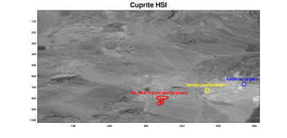
Figure 2: The Cuprite HSI of size $1024\times 614\times 186$. We exhibit the mean power in db over the 186 spectral bands.

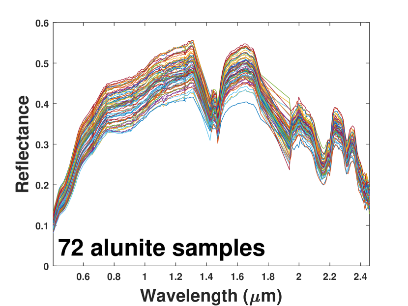
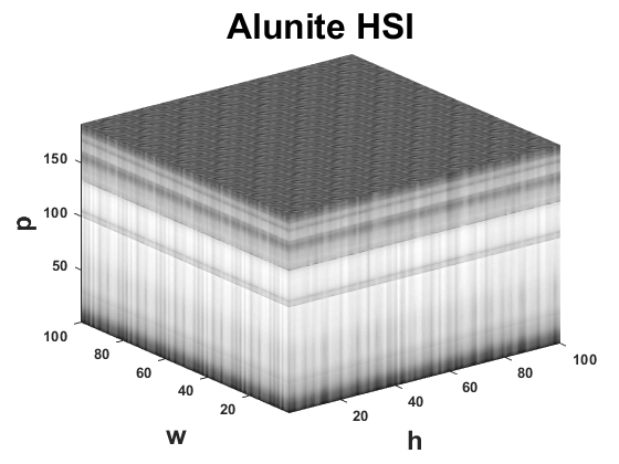
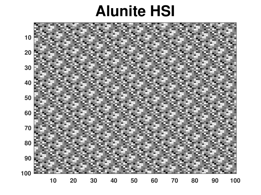
Figure 3: A $100\times 100\times 186$ “Alunite HSI” generated by 72 pure alunite samples picked from the Cuprite HSI (72 pixels from the solid red ellipses in Fig. 2). For the third image, we exhibit the mean power in db over the 186 spectral bands.

By referring to Fig. 8 in Swayze10245 , we picked 72 pure alunite pixels from the Cuprite HSI (72 pixels located inside the solid red ellipses in Fig. 2) and generate a $100\times 100\times 186$ HSI zone formed by these pixels. We shall call this small HSI zone as “Alunite HSI” (see Fig. 3), and which will be used for the target evaluations later. We incorporate, in this zone, seven target blocks (each of size $6\times 3$) with $\alpha\in[0.01,\,1]$ (all have the same $\alpha$ value), placed in long convoy formation all formed by the same target $\mathbf{t}$ that we picked from the Cuprite HSI and which will constitute our target of interest to be detected. The target $\mathbf{t}$ replaces a fraction $\alpha\in[0.01,\,1]$ from the background; specifically, the following values of $\alpha$ are considered: 0.01, 0.02, 0.05, 0.1, 0.3, 0.5, 0.8, and 1.
In the experiments, two kinds of target $\mathbf{t}$ are considered:

1. ‘$\mathbf{t}$’ that represents the buddingtonite target,

2. ‘$\mathbf{t}$’ that represents the kaolinite target.

More precisely, our detector $\left(\mathbf{A}_{t}\mathbf{C}\right)^{T}$ is evaluated on two target detection scenarios:

• Evaluation on an easy target (buddingtonite target): It has been noted by Gregg et al. Swayze10245 that the ammonia in the Tectosilicate mineral type, known as buddingtonite, has a distinct N-H combination absorption at 2.12 $\upmu$m, a position similar to that of the cellulose absorption in dried vegetation, from which it can be distinguished based on its narrower band width and asymmetry. Hence, the buddingtonite mineral can be considered as an “easy target” because it does not look like any other mineral with its distinct 2.12 $\upmu$m absorption (that is, it is easily recognized based on its unique 2.12 $\upmu$m absorption band).
  In the experiments, we consider the “buddingtonite” pixel at location (731, 469) in the Cuprite HSI (the center of the dash-dotted yellow circle in Fig. 2) as the buddingtonite target $\mathbf{t}$ to be incorporated in the Alunite HSI for $\alpha\in[0.01,\,1]$.

  

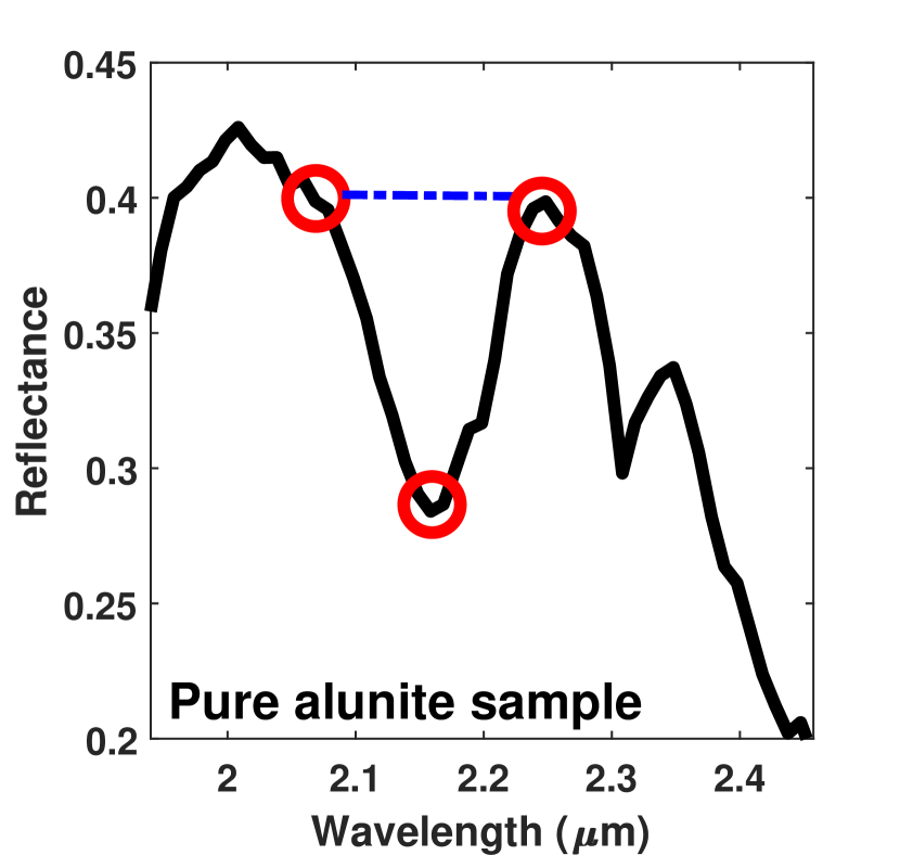
  (a)

  

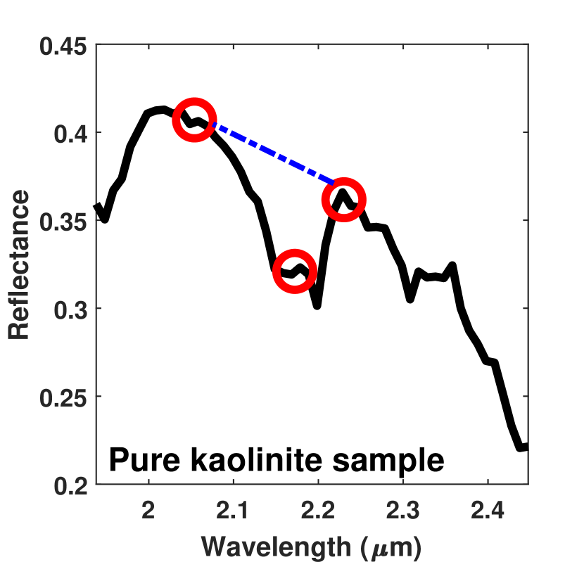
  (b)

  Figure 4: Three-point band depth images for both (a) alunite and (b) kaolinite.

• Evaluation on a challenging target (kaolinite target): The paradigm in military applications for hyperspectral imagery seems to center on finding the target but ignoring all the rest. Sometimes, that rest is important especially if the target is well matched to the surroundings. It has been shown by Gregg et al. Swayze10245 that both alunite and kaolinite minerals have overlapping spectral features, and thus, discrimination between these two minerals is a big challenge Swayze10245 ; doi:10.1029/2002JE001847 .
  In the experiments, we consider the “kaolinite” pixel at location (672, 572) in the Cuprite HSI (the center of the dotted blue circle in Fig. 2) as the kaolinite target $\mathbf{t}$ to be incorporated in the Alunite HSI for $\alpha\in[0.01,\,1]$.
  Figure 4a exhibits a three-point band depth image for our alunite background that shows the locations where an absorption feature, centered near 2.17 $\upmu$m, is expressed in spectra of surface materials. Figure 4b exhibits a three-point band depth image for our kaolinite target that shows the locations where an absorption feature, centered near 2.2 $\upmu$m, is expressed in spectra of surface materials. As we can observe, there is a subtle difference between the alunite and kaolinite three-point band depth images, showing that the successful spectral distinction between these two minerals is a very challenging task to achieve doi:10.1029/2002JE001847 .

4.1 Construction of the Target Dictionary $\mathbf{A}_{t}$

When $\mathbf{A}_{t}$ is constructed from background samples

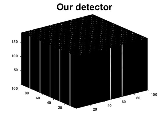
Figure 5: Evaluation of our detector $(\mathbf{A}_{t}\mathbf{C})^{T}$ for detecting the buddingtonite and kaolinite target (for $\alpha=1$) from the Alunite HSI when $\mathbf{A}_{t}$ is contsructed from some background pixels acquired from the Alunite HSI.

An important problem that requires a very careful attention is the construction of an appropriate dictionary $\mathbf{A}_{t}$ in order to capture the target well and distinguish it from the background. If $\mathbf{A}_{t}$ does not well represent the target of interest, our model in (2) may fail on discriminating the targets from the background. For example, Fig. 5 shows the detection results of our detector $(\mathbf{A}_{t}\mathbf{C})^{T}$ when $\mathbf{A}_{t}$ is constructed from some of the background pixels in the Alunite HSI. We can obviously observe that our detector is not able to capture the targets mainly because of the poor dictionary $\mathbf{A}_{t}$ constructed.

The target present in the HSI can be highly affected by the atmospheric conditions, sensor noise, material composition, and scene geometry. This may produce huge variations on the target spectra. In view of these real effects, it is very difficult to model the target dictionary $\mathbf{A}_{t}$ well. But this raises the question on “how these effects should be dealt with?”.

Some scenarios for modeling the target dictionary have been suggested in the literature. For example, by using physical models and the MODTRAN atmospheric modeling program Berk89 , target spectral signatures can be generated under various atmospheric conditions. For simplicity, we handle this problem in this work by exploiting target samples that are available in some online spectral libraries. More precisely, $\mathbf{A}_{t}$ can be constructed via the United States Geological Survey (USGS - Reston) spectral library Clark93 . However, the user can also deal with the Advanced Spaceborne Thermal Emission and Reflection (ASTER) spectral library Baldridge09 that includes data from the USGS spectral library, the Johns Hopkins University (JHU) spectral library, and the Jet Propulsion Laboratory (JPL) spectral library.

There are three buddingtonite samples available in the ASTER spectral library and will be considered to construct the dictionary $\mathbf{A}_{t}$ for the detection of our buddingtonite target (see Fig. 6 (first column)); whereas six kaolinite samples are available in the USGS spectral library and will be acquired to construct $\mathbf{A}_{t}$ for the detection of our kaolinite target (see Fig. 6 (second column)).

Note that the Alunite HSI, the buddingtonite target $\mathbf{t}$, the kaolinite target $\mathbf{t}$, and the buddingtonite/kaolinite target samples extracted from the online spectral libraries are all normalized to the values between 0 and 1.

For instance, it is usually difficult to find, for a specific given target, a sufficient number of available samples in the online spectral libraries. Hence, the dictionary $\mathbf{A}_{t}$ may still be not sufficiently selective and accurate. This is the most reason why problem (2) may fail to well capture the targets from the background.

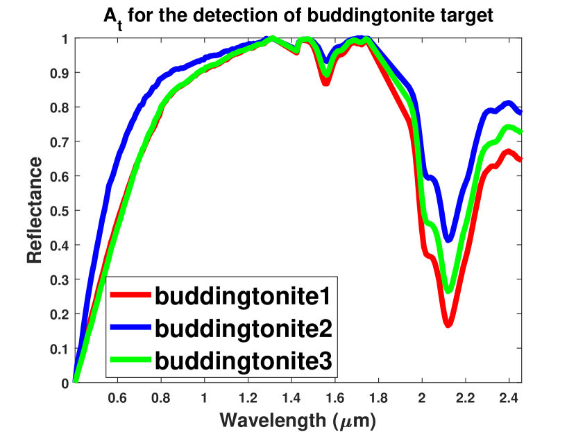
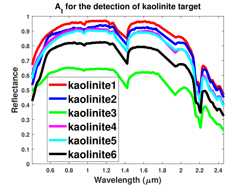
Figure 6: Target dictionaries for the detection of buddingtonite and kaolinite.

4.2 Target Detection Evaluation

We now aim to qualitatively evaluate the target detection performances of our detector $(\mathbf{A}_{t}\mathbf{C})^{T}$ on both the buddingtonite and kaolinite target detection scenarios, when $\mathbf{A}_{t}$ is constructed from target samples that are available in the online spectral libraries (from Fig. 6). As can be seen from Fig. 7, our detector is able to detect the buddingtonite targets with no false alarms until $\alpha\leq 0.1$ where a lot of false alarms appear.

For the detection of kaolinite, it was difficult to have a clean detection (without false alarms) even for high values of $\alpha$. This is to be expected since the kaolinite target is well matched to the alunite background (the kaolinite and alunite have overlapping spectral features), and hence, the discrimination between them is very challenging.

It is interesting to note (results omitted here) that if we consider $\mathbf{A}_{t}=\mathbf{t}$ (that is, we are searching for the exact signature $\mathbf{t}$ in the Alunite HSI), the buddingtonite and even the kaolinite targets are able to be detected with no false alarms for $0.1<\alpha\leq 1$. When $\alpha\leq 0.1$, a lot of false alarms appear, but the detection performances for both the buddingtonite and kaolinite targets remain better than to those in Fig. 7.

When $\mathbf{A}_{t}$ is constructed from target samples

$\bf\boldsymbol{\alpha}=1$

$\bf\boldsymbol{\alpha}=0.8$

$\bf\boldsymbol{\alpha}=0.5$

$\bf\boldsymbol{\alpha}=0.3$

$\bf\boldsymbol{\alpha}=0.1$

$\bf\boldsymbol{\alpha}=0.05$

$\bf\boldsymbol{\alpha}=0.02$

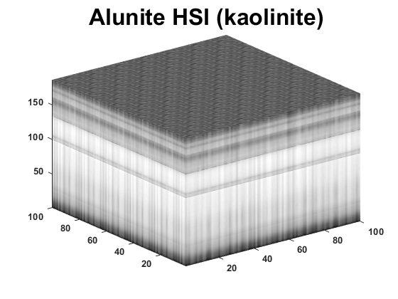
$\bf\boldsymbol{\alpha}=0.01$

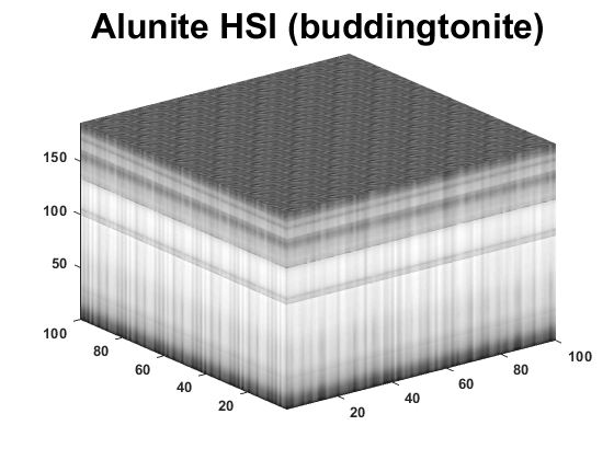
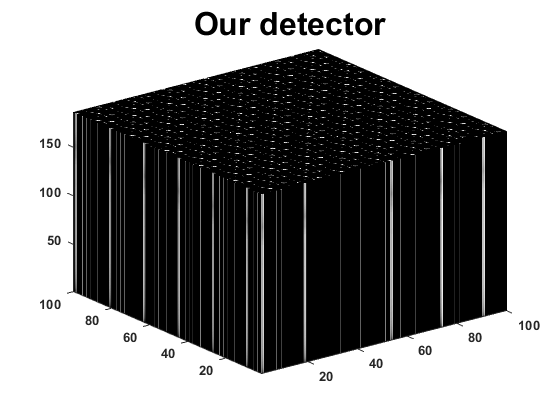
Figure 7: Evaluation of our detector $(\mathbf{A}_{t}\mathbf{C})^{T}$ for detecting the buddingtonite and kaolinite target (for $\alpha\in[0.01,\,1]$) when $\mathbf{A}_{t}$ is contsructed from target samples in the online spectral libraries.

5 Conclusion and Future Work

In this chapter, the well-known robust principal component analysis (RPCA) is exploited for target detection in hyperspectral imagery. By making assumptions similar to those used in RPCA, a given hyperspectral image (HSI) has been decomposed into the sum of a low-rank background HSI and a sparse target HSI that only contains the targets (with the background is suppressed) 8677268 . In order to alleviate the inadequacy of RPCA on distinguishing the true targets from the background, we have incorporated into the RPCA imaging, the prior target information that can often be provided to the user. In this regard, we have constructed a pre-learned target dictionary $\mathbf{A}_{t}$, and thus, the given HSI is decomposed as the sum of a low-rank background HSI $\mathbf{L}$ and a sparse target HSI $\left(\mathbf{A}_{t}\mathbf{C}\right)^{T}$, where $\mathbf{C}$ is a sparse activation matrix.

In this work, the sparse component $\left(\mathbf{A}_{t}\mathbf{C}\right)^{T}$ was only the object of interest and used directly for the detection. More precisely, the targets are deemed to be present at the non-zero entries of the sparse target HSI. Hence, a novel target detector is developed, which is simply a sparse HSI generated automatically from the original HSI, but containing only the targets of interest with the background is suppressed.

The detector is evaluated on real experiments, and the results of which demonstrate its effectiveness for hyperspectral target detection, especially on detecting targets that have overlapping spectral features with the background.

The $l_{1}$ norm regularizer, a continuous and convex surrogate, has been studied extensively in the literature Tibshirani96 ; 10.2307/3448465 and has been applied successfully to many applications including signal/image processing, biomedical informatics, and computer vision doi:10.1093/bioinformatics/btg308 ; 4483511 ; Beck:2009:FIS:1658360.1658364 ; 4799134 ; Ye:2012:SMB:2408736.2408739 . Although the $l_{1}$ norm based sparse learning formulations have achieved great success, they have been shown to be suboptimal in many cases CandAs2008 ; Zhanggg ; zhang2013 since the $l_{1}$ is still too far away from the ideal $l_{0}$ norm. To address this issue, many non-convex regularizers, interpolated between the $l_{0}$ norm and the $l_{1}$ norm, have been proposed to better approximate the $l_{0}$ norm. They include $l_{q}$ norm ($0<q<1$) Fourc1624 , Smoothly Clipped Absolute Deviation Fan01 , Log-Sum Penalty Candes08 , Minimax Concave Penalty zhang2010aa , Geman Penalty 392335 ; 5153291 , and Capped-$l_{1}$ penalty Zhanggg ; zhang2013 ; Gong12 .

• In this regard, from problem (2), it will be interesting to use other proxies than the $l_{2,1}$ norm, closer to $l_{2,0}$, in order to probably alleviate the $l_{2,1}$ artifact and also the manual selection problem of both $\tau$ and $\lambda$. But although the non-convex regularizers (penalties) are appealing in sparse learning, it remains a very big challenge to solve the corresponding non-convex optimization problems.

- (1) G. Shaw and D. Manolakis, “Signal processing for hyperspectral image exploitation,” IEEE Signal Processing Magazine, vol. 19, no. 1, pp. 12–16, Jan 2002.
- (2) D. Manolakis, D. Marden, and G. Shaw, “Hyperspectral image processing for automatic target detection applications,” Lincoln Laboratory Journal, vol. 14, no. 1, pp. 79–116, 2003.
- (3) D. G. Manolakis, R. B. Lockwood, and T. W. Cooley, Hyperspectral Imaging Remote Sensing: Physics, Sensors, and Algorithms, Cambridge University Press, 2016.
- (4) G. Shaw and D. Manolakis, “Signal processing for hyperspectral image exploitation,” IEEE Signal Processing Magazine, vol. 19, no. 1, pp. 12–16, Jan 2002.
- (5) L. Zhang, Q. Zhang, B. Du, X. Huang, Y. Y. Tang, and D. Tao, “Simultaneous spectral-spatial feature selection and extraction for hyperspectral images,” IEEE Transactions on Cybernetics, vol. 48, no. 1, pp. 16–28, Jan 2018.
- (6) L. Zhang, Q. Zhang, L. Zhang, D. Tao, X. Huang, and B. Du, “Ensemble manifold regularized sparse low-rank approximation for multiview feature embedding,” Pattern Recognition, vol. 48, no. 10, pp. 3102 – 3112, 2015, Discriminative Feature Learning from Big Data for Visual Recognition.
- (7) J. M. Bioucas-Dias, A. Plaza, G. Camps-Valls, P. Scheunders, N. Nasrabadi, and J. Chanussot, “Hyperspectral remote sensing data analysis and future challenges,” IEEE Geoscience and Remote Sensing Magazine, vol. 1, no. 2, pp. 6–36, June 2013.
- (8) Antonio Plaza, Jon Atli Benediktsson, Joseph W. Boardman, Jason Brazile, Lorenzo Bruzzone, Gustavo Camps-Valls, Jocelyn Chanussot, Mathieu Fauvel, Paolo Gamba, Anthony Gualtieri, Mattia Marconcini, James C. Tilton, and Giovanna Trianni, “Recent advances in techniques for hyperspectral image processing,” Remote Sensing of Environment, vol. 113, pp. S110 – S122, 2009, Imaging Spectroscopy Special Issue.
- (9) Q. Du, L. Zhang, B. Zhang, X. Tong, P. Du, and J. Chanussot, “Foreword to the special issue on hyperspectral remote sensing: Theory, methods, and applications,” IEEE Journal of Selected Topics in Applied Earth Observations and Remote Sensing, vol. 6, no. 2, pp. 459–465, April 2013.
- (10) P. D. Gader and J. Chanussot, “Understanding hyperspectral image and signal processing,” in John Wiley & Sons Inc, 2021.
- (11) Mauro Dalla Mura, Jon Atli Benediktsson, Jocelyn Chanussot, and Lorenzo Bruzzone, The Evolution of the Morphological Profile: from Panchromatic to Hyperspectral Images, pp. 123–146, Springer Berlin Heidelberg, Berlin, Heidelberg, 2011.
- (12) S. Prasad, L.M. Bruce, and J. Chanussot, Optical Remote Sensing: Advances in Signal Processing and Exploitation Techniques, Augmented Vision and Reality. Springer Berlin Heidelberg, 2011.
- (13) J. Chanussot, C. Collet, and K. Chehdi, Multivariate Image Processing, Augmented Vision and Reality. STE Ltd, UK and Wiley & Sons, USA, 2009.
- (14) Joana Maria Frontera Pons, Robust target detection for Hyperspectral Imaging, Ph.D. thesis, CentraleSupélec, 2014.
- (15) D. Manolakis, R. Lockwood, T. Cooley, and J. Jacobson, “Is there a best hyperspectral detection algorithm?,” Proc. SPIE 7334, Algorithms and Technologies for Multispectral, Hyperspectral, and Ultraspectral Imagery XV, 733402, 27 April 2009.
- (16) A. Villa, J. Chanussot, J. A. Benediktsson, and C. Jutten, “Unsupervised classification and spectral unmixing for sub-pixel labelling,” in 2011 IEEE International Geoscience and Remote Sensing Symposium, July 2011, pp. 71–74.
- (17) N. Yokoya, J. Chanussot, and A. Iwasaki, “Nonlinear unmixing of hyperspectral data using semi-nonnegative matrix factorization,” IEEE Transactions on Geoscience and Remote Sensing, vol. 52, no. 2, pp. 1430–1437, Feb 2014.
- (18) A. Villa, J. Chanussot, J. A. Benediktsson, and C. Jutten, “Spectral unmixing for the classification of hyperspectral images at a finer spatial resolution,” IEEE Journal of Selected Topics in Signal Processing, vol. 5, no. 3, pp. 521–533, June 2011.
- (19) G. A. Licciardi, A. Villa, M. M. Khan, and J. Chanussot, “Image fusion and spectral unmixing of hyperspectral images for spatial improvement of classification maps,” in 2012 IEEE International Geoscience and Remote Sensing Symposium, July 2012, pp. 7290–7293.
- (20) N. K. Patel, C. Patnaik, S. Dutta, A. M. Shekh, and A. J. Dave, “Study of crop growth parameters using airborne imaging spectrometer data,” International Journal of Remote Sensing, vol. 22, no. 12, pp. 2401–2411, 2001.
- (21) B. Datt, T. R. McVicar, T. G. van Niel, D. L. B. Jupp, and J. S. Pearlman, “Preprocessing EO-1 Hyperion hyperspectral data to support the application of agricultural indexes,” IEEE Transactions on Geoscience and Remote Sensing, vol. 41, pp. 1246–1259, June 2003.
- (22) B. Hörig, F. Kühn, F. Oschütz, and F. Lehmann, “HyMap hyperspectral remote sensing to detect hydrocarbons,” International Journal of Remote Sensing, vol. 22, pp. 1413–1422, May 2001.
- (23) D. Manolakis and G. Shaw, “Detection algorithms for hyperspectral imaging applications,” Signal Processing Magazine, IEEE, vol. 19, no. 1, pp. 29–43, 2002.
- (24) D. W. J. Stein, S. G. Beaven, L. E. Hoff, E. M. Winter, A. P. Schaum, and A. D. Stocker, “Anomaly detection from hyperspectral imagery,” IEEE Signal Processing Magazine, vol. 19, no. 1, pp. 58–69, Jan 2002.
- (25) M. T. Eismann, A. D. Stocker, and N. M. Nasrabadi, “Automated hyperspectral cueing for civilian search and rescue,” Proceedings of the IEEE, vol. 97, no. 6, pp. 1031–1055, June 2009.
- (26) D. Manolakis, E. Truslow, M. Pieper, T. Cooley, and M. Brueggeman, “Detection algorithms in hyperspectral imaging systems: An overview of practical algorithms,” IEEE Signal Processing Magazine, vol. 31, no. 1, pp. 24–33, Jan 2014.
- (27) J. Frontera-Pons, F. Pascal, and J.-P. Ovarlez, “Adaptive nonzero-mean Gaussian detection,” IEEE Transactions on Geoscience and Remote Sensing, vol. 55, no. 2, pp. 1117–1124, Feb 2017.
- (28) J. Frontera-Pons, M. A. Veganzones, F. Pascal, and J.-P. Ovarlez, “Hyperspectral anomaly detectors using robust estimators,” IEEE Journal of Selected Topics in Applied Earth Observations and Remote Sensing, vol. 9, no. 2, pp. 720–731, Feb 2016.
- (29) J. Frontera-Pons, J.-P. Ovarlez, and F. Pascal, “Robust anmf detection in noncentered impulsive background,” IEEE Signal Processing Letters, vol. 24, no. 12, pp. 1891–1895, Dec 2017.
- (30) J. Frontera-Pons, M. A. Veganzones, S. Velasco-Forero, F. Pascal, J. P. Ovarlez, and J. Chanussot, “Robust anomaly detection in hyperspectral imaging,” in 2014 IEEE Geoscience and Remote Sensing Symposium, July 2014, pp. 4604–4607.
- (31) R. M. Cavalli, G. A. Licciardi, and J. Chanussot, “Detection of anomalies produced by buried archaeological structures using nonlinear principal component analysis applied to airborne hyperspectral image,” IEEE Journal of Selected Topics in Applied Earth Observations and Remote Sensing, vol. 6, no. 2, pp. 659–669, April 2013.
- (32) D. Manolakis, G. Shaw, and N. Keshava, “Comparative analysis of hyperspectral adaptive matched filter detectors,” Proc. SPIE 4049, Algorithms for Multispectral, Hyperspectral, and Ultraspectral Imagery VI, vol. 2, Aug 2000.
- (33) N. M. Nasrabadi, “Regularized spectral matched filter for target recognition in hyperspectral imagery,” IEEE Signal Processing Letters, vol. 15, pp. 317–320, 2008.
- (34) S. Kraut and L. L. Scharf, “The CFAR adaptive subspace detector is a scale-invariant GLRT,” Signal Processing, IEEE Transactions on, vol. 47, no. 9, pp. 2538–2541, 1999.
- (35) E. J. Kelly, “An adaptive detection algorithm,” Aerospace and Electronic Systems, IEEE Transactions on, vol. 23, no. 1, pp. 115–127, November 1986.
- (36) O. Ledoit and M. Wolf, “A well-conditioned estimator for large-dimensional covariance matrices,” Journal of Multivariate Analysis, vol. 88, no. 2, pp. 365 – 411, 2004.
- (37) O. Ledoit and M. Wolf, “Honey, i shrunk the sample covariance matrix,” UPF Economics and Business Working Paper, , no. 691, 2003.
- (38) A. W. Bitar, J.-P. Ovarlez, and L.-F. Cheong, “Sparsity-Based Cholesky Factorization and Its Application to Hyperspectral Anomaly Detection,” in IEEE Workshop on Computational Advances in Multi-Sensor Adaptive Processing (CAMSAP-17), Curaçao, Dutch Antilles, December 2017.
- (39) Y. Chen, A. Wiesel, and A. O. Hero, “Robust shrinkage estimation of high-dimensional covariance matrices,” in 2010 IEEE Sensor Array and Multichannel Signal Processing Workshop, Oct 2010, pp. 189–192.
- (40) F. Pascal and Y. Chitour, “Shrinkage covariance matrix estimator applied to stap detection,” in 2014 IEEE Workshop on Statistical Signal Processing (SSP), June 2014, pp. 324–327.
- (41) F. Pascal, Y. Chitour, and Y. Quek, “Generalized robust shrinkage estimator and its application to stap detection problem,” IEEE Transactions on Signal Processing, vol. 62, no. 21, pp. 5640–5651, Nov 2014.
- (42) G. Healey and D. Slater, “Models and methods for automated material identification in hyperspectral imagery acquired under unknown illumination and atmospheric conditions,” IEEE Transactions on Geoscience and Remote Sensing, vol. 37, no. 6, pp. 2706–2717, 1999.
- (43) B. Thai and G. Healey, “Invariant subpixel material detection in hyperspectral imagery,” IEEE Transactions on Geoscience and Remote Sensing, vol. 40, no. 3, pp. 599–608, 2002.
- (44) J. Wright, A. Y. Yang, A. Ganesh, S. S. Sastry, and Y. Ma, “Robust face recognition via sparse representation,” IEEE Transactions on Pattern Analysis and Machine Intelligence, vol. 31, no. 2, pp. 210–227, Feb 2009.
- (45) R. Basri and D. W. Jacobs, “Lambertian reflectance and linear subspaces,” IEEE Transactions on Pattern Analysis and Machine Intelligence, vol. 25, no. 2, pp. 218–233, Feb 2003.
- (46) J. K. Pillai, V. M. Patel, and R. Chellappa, “Sparsity inspired selection and recognition of iris images,” in 2009 IEEE 3rd International Conference on Biometrics: Theory, Applications, and Systems, Sept 2009, pp. 1–6.
- (47) X. Hang and F.-X Wu, “Sparse representation for classification of tumors using gene expression data,” in Journal of Biomedicine and Biotechnology, 2009, p. 6.
- (48) Z. Guo, T. Wittman, and S. Osher, “L1 unmixing and its application to hyperspectral image enhancement,” 2009.
- (49) J. M. Bioucas-Dias, A. Plaza, N. Dobigeon, M. Parente, Q. Du, P. Gader, and J. Chanussot, “Hyperspectral unmixing overview: Geometrical, statistical, and sparse regression-based approaches,” IEEE Journal of Selected Topics in Applied Earth Observations and Remote Sensing, vol. 5, no. 2, pp. 354–379, April 2012.
- (50) Y. Chen, N. M. Nasrabadi, and T. D. Tran, “Sparse representation for target detection in hyperspectral imagery,” IEEE Journal of Selected Topics in Signal Processing, vol. 5, no. 3, pp. 629–640, June 2011.
- (51) Y. Zhang, B. Du, and L. Zhang, “A sparse representation-based binary hypothesis model for target detection in hyperspectral images,” IEEE Transactions on Geoscience and Remote Sensing, vol. 53, no. 3, pp. 1346–1354, March 2015.
- (52) A. W. Bitar, L. Cheong, and J. Ovarlez, “Target and background separation in hyperspectral imagery for automatic target detection,” in 2018 IEEE International Conference on Acoustics, Speech and Signal Processing (ICASSP), April 2018, pp. 1598–1602.
- (53) A. W. Bitar, L. Cheong, and J. Ovarlez, “Sparse and low-rank matrix decomposition for automatic target detection in hyperspectral imagery,” IEEE Transactions on Geoscience and Remote Sensing, vol. 57, no. 8, pp. 5239–5251, Aug 2019.
- (54) E. J. Candès, X. Li, Y. Ma, and J. Wright, “Robust principal component analysis?,” J. ACM, vol. 58, no. 3, pp. 11:1–11:37, June 2011.
- (55) J. Wright, G. Arvind, R. Shankar, P. Yigang, and Y. Ma, “Robust principal component analysis: Exact recovery of corrupted low-rank matrices via convex optimization,” in Advances in Neural Information Processing Systems 22, Y. Bengio, D. Schuurmans, J. D. Lafferty, C. K. I. Williams, and A. Culotta, Eds., pp. 2080–2088. Curran Associates, Inc., 2009.
- (56) S.-Y. Chen, S. Yang, K. KalpakiS, and C. Chang, “Low-rank decomposition-based anomaly detection,” in Proc. SPIE 8743 Algorithms and Technologies for Multispectral, Hyperspectral, and Ultraspectral Imagery XIX, 2013, pp. 87430 –87430 –7.
- (57) Y. Zhang, B. Du, L. Zhang, and S. Wang, “A low-rank and sparse matrix decomposition-based Mahalanobis distance method for hyperspectral anomaly detection,” IEEE Transactions on Geoscience and Remote Sensing, vol. 54, no. 3, pp. 1376–1389, March 2016.
- (58) Y. Xu, Z. Wu, J. Li, A. Plaza, and Z. Wei, “Anomaly detection in hyperspectral images based on low-rank and sparse representation,” IEEE Transactions on Geoscience and Remote Sensing, vol. 54, no. 4, pp. 1990–2000, April 2016.
- (59) Y. Xu, Z. Wu, J. Chanussot, and Z. Wei, “Joint reconstruction and anomaly detection from compressive hyperspectral images using mahalanobis distance-regularized tensor rpca,” IEEE Transactions on Geoscience and Remote Sensing, vol. 56, no. 5, pp. 2919–2930, May 2018.
- (60) Y. Xu, Z. Wu, J. Chanussot, M. Dalla Mura, A. L. Bertozzi, and Z. Wei, “Low-rank decomposition and total variation regularization of hyperspectral video sequences,” IEEE Transactions on Geoscience and Remote Sensing, vol. 56, no. 3, pp. 1680–1694, March 2018.
- (61) A. W. Bitar, L. Cheong, and J. Ovarlez, “Simultaneous sparsity-based binary hypothesis model for real hyperspectral target detection,” in 2017 IEEE International Conference on Acoustics, Speech and Signal Processing (ICASSP), March 2017, pp. 4616–4620.
- (62) M. A. Veganzones, M. Sim es, G. Licciardi, N. Yokoya, J. M. Bioucas-Dias, and J. Chanussot, “Hyperspectral super-resolution of locally low rank images from complementary multisource data,” IEEE Transactions on Image Processing, vol. 25, no. 1, pp. 274–288, Jan 2016.
- (63) G. Liu, Z. Lin, S. Yan, J. Sun, Y. Yu, and Y. Ma, “Robust recovery of subspace structures by low-rank representation,” IEEE Transactions on Pattern Analysis and Machine Intelligence, vol. 35, no. 1, pp. 171–184, Jan 2013.
- (64) Z. Zhou, X. Li, J. Wright, E. Cand s, and Y. Ma, “Stable principal component pursuit,” in 2010 IEEE International Symposium on Information Theory, June 2010, pp. 1518–1522.
- (65) Z. Chen and D. P. W. Ellis, “Speech enhancement by sparse, low-rank, and dictionary spectrogram decomposition,” in 2013 IEEE Workshop on Applications of Signal Processing to Audio and Acoustics, Oct 2013, pp. 1–4.
- (66) P. Sun and J. Qin, “Low-rank and sparsity analysis applied to speech enhancement via online estimated dictionary,” IEEE Signal Processing Letters, vol. 23, no. 12, pp. 1862–1866, Dec 2016.
- (67) J.-F. Cai, E. J. Candès, and Z. Shen, “A singular value thresholding algorithm for matrix completion,” SIAM J. on Optimization, vol. 20, no. 4, pp. 1956–1982, Mar. 2010.
- (68) E. J. Candes and B. Recht, “Exact low-rank matrix completion via convex optimization,” in 2008 46th Annual Allerton Conference on Communication, Control, and Computing, Sept 2008, pp. 806–812.
- (69) A.S. Lewis, “The mathematics of eigenvalue optimization,” Mathematical Programming, vol. 97, no. 1, pp. 155–176, Jul 2003.
- (70) G.A. Watson, “Characterization of the subdifferential of some matrix norms,” Linear Algebra and its Applications, vol. 170, pp. 33 – 45, 1992.
- (71) Stephen Boyd, Neal Parikh, Eric Chu, Borja Peleato, and Jonathan Eckstein, “Distributed optimization and statistical learning via the alternating direction method of multipliers,” Found. Trends Mach. Learn., vol. 3, no. 1, pp. 1–122, Jan. 2011.
- (72) Junfeng Yang, Wotao Yin, Yin Zhang, and Yilun Wang, “A fast algorithm for edge-preserving variational multichannel image restoration,” SIAM Journal on Imaging Sciences, vol. 2, no. 2, pp. 569–592, 2009.
- (73) G. A. Swayze, R. N. Clark, A. F. H. Goetz, K. E. Livo, G. N. Breit, F. A. Kruse, S. J. Sutley, L. W. Snee, H. A. Lowers, J. L. Post, R. E. Stoffregen, and R. P. Ashley, “Mapping advanced argillic alteration at cuprite, nevada, using imaging spectroscopy,” Economic Geology, vol. 109, no. 5, pp. 1179, 2014.
- (74) Airbone Visible / Infrared Imaging Spectrometer, “https://aviris.jpl.nasa.gov,” .
- (75) G. A. Swayze, R. N. Clark, A. F. H. Goetz, T. G. Chrien, and N. S. Gorelick, “Effects of spectrometer band pass, sampling, and signal-to-noise ratio on spectral identification using the tetracorder algorithm,” Journal of Geophysical Research: Planets, vol. 108, no. E9, 2003, 5105.
- (76) Roger N. Clark, Gregg A. Swayze, K. Eric Livo, Raymond F. Kokaly, Steve J. Sutley, J. Brad Dalton, Robert R. McDougal, and Carol A. Gent, “Imaging spectroscopy: Earth and planetary remote sensing with the usgs tetracorder and expert systems,” Journal of Geophysical Research: Planets, vol. 108, no. E12.
- (77) A. Berk, L. Bernstein, and D. Robertson, “MODTRAN: A moderate resolution model for LOWTRAN 7,” Tech. Rep. GL-TR-90-0122, Geophysics Laboratory, Bedford, MA, 1989.
- (78) R. N. Clark, G. A. Swayze, A. J. Gallagher, T. V. V. King, and W. M. Calvin, “The U. S. Geological Survey, Digital Spectral Library: Version 1: 0.2 to 3.0 micros,” Open file report, U.S. Geological Survey, 1993.
- (79) A. M. Baldridge, S. J. Hook, C. I. Grove, and G. Rivera, “The ASTER Spectral Library Version 2.0,” Remote Sensing of Environment, vol. 113, pp. 711–715, 2009.
- (80) R. Tibshirani, “Regression shrinkage and selection via the lasso.,” Journal of the Royal Statistical Society. Series B (Methodological), vol. 58, no. 1, pp. 267–288, 1996.
- (81) B. Efron, T. Hastie, I. Johnstone, and R. Tibshirani, “Least angle regression,” The Annals of Statistics, vol. 32, no. 2, pp. 407–451, 2004.
- (82) S. K. Shevade and S. S. Keerthi, “A simple and efficient algorithm for gene selection using sparse logistic regression,” Bioinformatics, vol. 19, no. 17, pp. 2246–2253, 2003.
- (83) Amir Beck and Marc Teboulle, “A fast iterative shrinkage-thresholding algorithm for linear inverse problems,” SIAM J. Img. Sci., vol. 2, no. 1, pp. 183–202, Mar. 2009.
- (84) S. J. Wright, R. D. Nowak, and M. A. T. Figueiredo, “Sparse reconstruction by separable approximation,” IEEE Transactions on Signal Processing, vol. 57, no. 7, pp. 2479–2493, July 2009.
- (85) Jieping Ye and Jun Liu, “Sparse methods for biomedical data,” SIGKDD Explor. Newsl., vol. 14, no. 1, pp. 4–15, Dec. 2012.
- (86) Emmanuel J. Candès, Michael B. Wakin, and Stephen P. Boyd, “Enhancing sparsity by reweighted minimization,” Journal of Fourier Analysis and Applications, vol. 14, no. 5, pp. 877–905, Dec 2008.
- (87) Tong Zhang, “Analysis of multi-stage convex relaxation for sparse regularization,” J. Mach. Learn. Res., vol. 11, pp. 1081–1107, Mar. 2010.
- (88) Tong Zhang, “Multi-stage convex relaxation for feature selection,” Bernoulli, vol. 19, no. 5B, pp. 2277–2293, 11 2013.
- (89) S. Foucart and M.J Lai, “Sparsest solutions of underdetermined linear systems via -minimization for ,” Applied and Computational Harmonic Analysis, vol. 26, no. 3, pp. 395–407, 2009.
- (90) J. Fan and R. Li, “Variable selection via nonconcave penalized likelihood and its oracle properties,” Journal of the American Statistical Association, vol. 96, no. 456, pp. 1348–1360, 2001.
- (91) E. Candès, M. B. Wakin, and S. P. Boyd, “Enhancing sparsity by reweighted l1 minimization,” Journal of Fourier Analysis and Applications, vol. 14, no. 5, pp. 877–905, 2008.
- (92) Cun-Hui Zhang, “Nearly unbiased variable selection under minimax concave penalty,” Ann. Statist., vol. 38, no. 2, pp. 894–942, 04 2010.
- (93) D. Geman and Chengda Yang, “Nonlinear image recovery with half-quadratic regularization,” IEEE Transactions on Image Processing, vol. 4, no. 7, pp. 932–946, Jul 1995.
- (94) J. Trzasko and A. Manduca, “Relaxed conditions for sparse signal recovery with general concave priors,” IEEE Transactions on Signal Processing, vol. 57, no. 11, pp. 4347–4354, Nov 2009.
- (95) P. Gong, J. Ye, and C. Zhang, “Multi-stage multi-task feature learning,” in Advances in Neural Information Processing Systems 25, F. Pereira, C. J. C. Burges, L. Bottou, and K. Q. Weinberger, Eds., pp. 1988–1996. Curran Associates, Inc., 2012.