Semi-bandit Optimization in the Dispersed Setting

Abstract

The goal of data-driven algorithm design is to obtain high-performing algorithms for specific application domains using machine learning and data. Across many fields in AI, science, and engineering, practitioners will often fix a family of parameterized algorithms and then optimize those parameters to obtain good performance on example instances from the application domain. In the online setting, we must choose algorithm parameters for each instance as they arrive, and our goal is to be competitive with the best fixed algorithm in hindsight.

There are two major challenges in online data-driven algorithm design. First, it can be computationally expensive to evaluate the loss functions that map algorithm parameters to performance, which often require the learner to run a combinatorial algorithm to measure its performance. Second, the losses can be extremely volatile and have sharp discontinuities. However, we show that in many applications, evaluating the loss function for one algorithm choice can sometimes reveal the loss for a range of similar algorithms, essentially for free. We develop online optimization algorithms capable of using this kind of extra information by working in the semi-bandit feedback setting. Our algorithms achieve regret bounds that are essentially as good as algorithms under full-information feedback and are significantly more computationally efficient. We apply our semi-bandit results to obtain the first provable guarantees for data-driven algorithm design for linkage-based clustering and we improve the best regret bounds for designing greedy knapsack algorithms.

1 Introduction

Overview.

This paper concerns data-driven algorithm design for combinatorial settings, which is an important area at the intersection of machine learning and computing that has been long of interest to the AI community [23, 41, 29, 18]. However, until recently, most algorithm design procedures did not have any provable guarantees on their performance, especially in the realistic online scenario. The first general online data-driven algorithm design procedures with regret bounds were given by Balcan et al. [11], who studied the problem under full-information and bandit feedback regimes. We develop efficient semi-bandit algorithms that achieve nearly the same regret as their full information algorithms, while being as efficient as their bandit algorithms.

The goal of data-driven algorithm design is to use machine learning and data to decide what algorithm to use from a large (typically parametrized) family of algorithms for a given problem domain. For example, we may want to decide which clustering algorithm to use from a large family of clustering procedures in order to obtain the highest quality results. We are concerned with the online setting, where at each round the learner chooses an algorithm from the family and receives a new instance of the problem. The problem is characterized by a loss function that measures the performance of each algorithm in the family for the given instance, and the goal is to select algorithms so that the cumulative performance of the learner is nearly as good as the best algorithm in hindsight for that sequence of problems.

The major challenge in these settings is that it is potentially computationally expensive for the learner to characterize the loss function for each round, since each run of the algorithm reveals the value of the loss function for just the selected parameters. Moreover, for combinatorial problems, small differences between two algorithms can lead to a cascade of changes in their behavior and significantly change their performance. However, when the algorithm family is parameterized, it can often be shown that the losses—though highly nonconvex in general—are at least piecewise Lipschitz in the algorithm parameters, so we can phrase the problem as online optimization of piecewise Lipschitz functions.

Prior work on piecewise Lipschitz optimization was limited to two extreme feedback regimes: Either the learner carries out a computationally expensive process to obtain full-information feedback (i.e., it observes the loss of every algorithm in the family on each instance), or accepts suboptimal regret bounds to work in the bandit feedback setting (i.e., it only observes the loss of one algorithm for each instance). This creates a tradeoff between computational efficiency and good regret bounds. However, many data-driven algorithm design problems exhibit rich additional structure that is ignored by these two approaches. We show that, surprisingly, evaluating the loss function for a single algorithm can sometimes reveal the loss for a range of similar algorithms, essentially for free; in the context of the loss function, we show that an entire Lipschitz region can often be learned at once. This motivates us to define a new learning model, which we call the semi-bandit feedback setting for learning piecewise Lispchitz functions. Our new results in this model achieve the best of both worlds: we can efficiently obtain the necessary feedback while also having regret bounds that are nearly as good as under full-information.

We instantiate our results for data-driven algorithm design on two combinatorial problems. These are machine learning problems where the goal is to learn an optimal algorithm, rather than a prediction rule. Our results for optimizing over a family of greedy knapsack algorithms improve over the procedures of Balcan et al. [11], Gupta and Roughgarden [21], and Cohen-Addad and Kanade [16] by simultaneously being more efficient and having tighter regret bounds. We also provide the first online data-driven algorithm design procedures for a rich family of linkage based clustering algorithms introduced by Balcan et al. [9] that interpolates between single and complete linkage, which are algorithms that are widely used in practice [6, 34, 40] and known to perform optimally in many settings [5, 8, 7, 20]. Balcan et al. [9] consider the data-driven algorithm design problem for this family of algorithms in the batch setting, rather than the online setting, where they model the application domain as a distribution over problem instances, the goal is to find the algorithm with the highest expected performance given an i.i.d. sample from the distribution as training data.

Problem Setup.

We study the problem of online piecewise Lipschitz optimization. The learning protocol is as follows: on each round $t$, the learner chooses a parameter $\rho_{t}$ belonging to a $d$-dimensional parameter space $\mathcal{C}\subset\mathbb{R}^{d}$, the adversary chooses a piecewise Lipschitz loss function $\ell_{t}:\mathcal{C}\to[0,1]$, and the learner incurs a loss equal to $\ell_{t}(\rho_{t})$. A function $\ell_{t}:\mathcal{C}\to[0,1]$ is piecewise $L$-Lipschitz if we can partition the parameter space $\mathcal{C}$ into regions such that $\ell_{t}$ is $L$-Lipschitz when restricted to each region. Many important instances of data-driven algorithm design require optimizing piecewise Lipschitz functions, including greedy combinatorial algorithms [21], clustering algorithms and SDP-rounding schemes [9], branch and bound mixed integer program solvers [10], initialization procedures for $k$-means clustering [12], and various auction design problems [13]. In these problems, the family of algorithms is parameterized and each parameter $\rho\in\mathcal{C}$ corresponds to one algorithm. We suppose that on each round $t$ there is a partition $A^{(t)}_{1},\dots,A^{(t)}_{M}$ of the parameter space $\mathcal{C}$, called the feedback system. If the learner’s parameter $\rho_{t}$ belongs to the set $A^{(t)}_{i}$, then they observe both the set $A^{(t)}_{i}$ as well as the loss $\ell_{t}(\rho)$ for every $\rho\in A^{(t)}_{i}$. We consider the uninformed setting, where the learner does not know the feedback system for round $t$ in advance of selecting a parameter. For simplicity, we consider oblivious adversaries that choose their sequence of loss functions $\ell_{1},\ell_{2},\dots$ adversarially, but before the interaction with the learner begins. The learner’s goal is to minimize regret, which is the difference between their total accumulated loss and that of the best parameter in hindsight: $\sum_{t=1}^{T}\ell_{t}(\rho_{t})-\min_{\rho\in\mathcal{C}}\sum_{t=1}^{T}\ell_{t}(\rho)$.

Throughout the paper, we use the notation $\tilde{O}(\cdot)$ to optionally suppress all logarithmic terms and dependence on parameters other than the time horizon $T$ and the dimension of the parameter space $d$.

Main Results and Techniques.

Semi-bandit Regret Bounds in the Dispersed Setting. It is not always possible to achieve sub-linear regret for piecewise Lipschitz loss functions [30, 14, 32]. Balcan et al. [11] provide regret bounds in the full-information and bandit feedback settings under a dispersion condition that roughly measures the number of discontinuous functions in any ball of a given radius, and which is satisfied for a diverse collection of combinatorial algorithm configuration problems. In this paper, we introduce a related and more general version of this condition that captures what is asymptotically important for our regret bounds.

Definition 1.

The sequence of loss functions $\ell_{1},\ell_{2},\dots$ is $\beta$-point-dispersed for the Lipschitz constant $L$ if for all $T$ and for all $\epsilon\geq T^{-\beta}$, we have that, in expectation, the maximum number of functions among $\ell_{1},\dots,\ell_{T}$ that fail the $L$-Lipschitz condition for any pair of points at distance $\epsilon$ in $\mathcal{C}$ is at most $\tilde{O}(\epsilon T)$. That is, for all $T$ and for all $\epsilon\geq T^{-\beta}$, we have $\operatorname{\mathbb{E}}\bigl{[}\max_{\rho,\rho^{\prime}}\bigl{|}\{t\in[T]\,:\,|\ell_{t}(\rho)-\ell_{t}(\rho^{\prime})|>L\|\rho-\rho^{\prime}\|_{2}\}\bigr{|}\bigr{]}=\tilde{O}(\epsilon T).$ where the max is taken over all $\rho,\rho^{\prime}\in\mathcal{C}:\|\rho-\rho^{\prime}\|_{2}\leq\epsilon$.

Note that the righthandside $\tilde{O}(\epsilon T)$ is roughly the number $L$-Lipschitz failures one would expect across $T$ functions for a pair of points at distance $\epsilon$ if Lipschitz failures are distributed reasonably randomly, and their probability of occuring between a pair of points at distance $\epsilon$ is roughly proportional to $\epsilon$. The definition of $\beta$-dispersion measures how small $\epsilon$ can be while maintaining the correctness of this rough bound for the loss functions $\ell_{i}$.

In our applications, the sequence of loss functions will be chosen by a smoothed adversary, in the sense of Spielman and Teng [36]. Informally, the discontinuity locations of the functions chosen by a smoothed adversary are randomly perturbed. The expectation in Definition 1 is over this randomness in the sequence of loss functions. (Balcan et al. [11] also show examples where sufficient randomness can arise from the algorithm itself, rather than smoothness constraints on the adversary.) In all of our applications, we prove $\beta$-dispersion with $\beta=1/2$. We provide an algorithm for online piecewise Lipschitz optimization under semi-bandit feedback whose regret is characterized by the $\beta$-dispersion parameter of the losses. In Section 2, we prove the following result:

Theorem 2.

Let $\mathcal{C}\subset\mathbb{R}^{d}$ be a bounded parameter space and $\ell_{1},\ell_{2},\dots:\mathcal{C}\to[0,1]$ be piecewise Lipschitz functions that are $\beta$-point-dispersed. Running the continuous Exp3-SET algorithm (Algorithm 1) under semi-bandit feedback with an appropriate parameter $\lambda$ has expected regret bounded by $\operatorname{\mathbb{E}}\bigl{[}\sum_{t=1}^{T}\ell_{t}(\rho_{t})-\ell_{t}(\rho^{*})\bigr{]}\leq\tilde{O}\bigl{(}\sqrt{dT}+T^{1-\beta}\bigr{)}.$

In comparison, the bandit-feedback algorithm of Balcan et al. [11] has expected regret bounded by $\tilde{O}(dT^{\frac{d+1}{d+2}}3^{d}+T^{1-\beta})$. Even in one-dimensional problems, this bound is $\tilde{O}(T^{2/3}+T^{1-\beta})$, which is worse than our results. Under different assumptions, the bandit algorithm of Cohen-Addad and Kanade [16] has $\tilde{O}(T^{2/3})$ regret for the special case of one-dimensional piecewise constant functions.

General Tools for Verifying Dispersion. We also provide general tools for proving that a sequence of piecewise Lipschitz functions satisfies dispersion. When the sequence $\ell_{1},\ell_{2},\dots$ is random, we can usually directly bound the expected number of loss functions that are not $L$-Lipschitz between any fixed pair of points $\rho$ and $\rho^{\prime}$ with $\|\rho-\rho^{\prime}\|_{2}\leq\epsilon$ by $\tilde{O}(T\epsilon)$. However, this does not imply that the functions are $\beta$-point-dispersed, since the expected number of non-Lipschitz functions between the worst pair of points at distance $\epsilon$ will typically be larger than the expected number for any fixed pair. Building on uniform convergence from learning theory [35], we show that if each loss function has a one-dimensional domain, at most $K$ discontinuities and any interval of radius $\epsilon$ has at most $\tilde{O}(T\epsilon)$ non-Lipschitz functions in expectation, then the expected number of non-Lipschitz losses on the worst interval of length $\epsilon$ is at most $\tilde{O}(T\epsilon+\sqrt{T\log(TK)})$. This implies that for all pairs of points at distance $\epsilon$, at most $O(T\epsilon+\sqrt{T\log(TK)})$ functions are non-Lipschitz between them and demonstrates $\beta$-dispersion with $\beta=1/2$. Our result gives an exponential improvement in the dependence on $K$ compared to the results of Balcan et al. [11], who upper bound the expected number of non-Lipschitz losses in the worst interval of length $\epsilon$ by $\tilde{O}(TK\epsilon+K\sqrt{T\log(TK)})$.

Semi-bandit Online Data-driven Algorithm Design. In Section 4, we combine our general regret analysis from Theorem 2 together with application-specific dispersion analysis to obtain practical data-driven algorithm design procedures for linkage-based clustering and the knapsack problem. In both applications, we show that the discontinuities of each loss function are the roots of polynomials depending on the corresponding problem instance, and that the roots are dispersed under mild smoothness assumptions on the adversary. We obtain the first online data-driven algorithm design procedures for linkage based clustering, and algorithm design procedures for the knapsack problem with substantial computational improvements over the prior work, while at the same time achieving nearly the same regret bound.

Explicit Comparison for Knapsack. To highlight the benefits of our new learning model and results applied to data-driven algorithm design, we give an explicit comparison of the computational complexity for obtaining different types of feedback and the corresponding regret bounds for the family of greedy knapsack algorithms introduced in Section 4.1. In each round of the online game, the algorithm chooses a parameter $\rho$, a new knapsack instance with $n$ items arrives, and our goal is for the total value of items selected by the learner to be close to the total value of the best fixed parameter $\rho$ in hindsight. We compare our results to the best prior full-information and bandit feedback procedures.

• Full-information. Balcan et al. [11] show that the exponentially weighted forecaster with full-information feedback achieves a regret bound of $\tilde{O}(n^{2}\sqrt{T})$. Our tighter analysis improves the bound to $\tilde{O}(\sqrt{T})$. Obtaining full-information feedback has a total cost of $O(n^{3}\log n)$ time per round.

• Bandit Feedback. The discretization-based bandit algorithm of Balcan et al. [11] has regret $\tilde{O}(T^{2/3}n^{2})$, but only requires $O(n\log n)$ time per round.

• Semi-bandit Feedback. In this paper we give an algorithm whose regret is $\tilde{O}(n\sqrt{T})$ using semi-bandit feedback obtainable in time $O(n\log n)$ per round. Note that our algorithm is as efficient as the bandit-feedback algorithm, yet its regret is only larger by a factor of $n$

Related Work.

There is a rich literature on data-driven algorithm design. Most prior work focuses on the statistical setting, where the learner is given a large iid sample of problem instances from some distribution, and the goal is to find the algorithm with the best performance in expectation. Gupta and Roughgarden [21] introduced this formal setting and provide sample complexity results for several families of greedy algorithms. Balcan et al. [9] consider semidefinite rounding schemes for integer quadratic programs and linkage based clustering algorithms, Balcan et al. [10] consider learning the best branch and bound algorithms for mixed integer programs, and Balcan et al. [12] consider learning the best initialization procedures for $k$-means clustering. Aamand et al. [1] and Hsu et al. [24] use learned algorithms for streaming frequency estimation. Indyk et al. [25] study the problem of using a learned sketching matrix to improve low-rank approximation algorithms. Dong et al. [19] use learned space partitions to improve nearest neighbor search. In addition to these formal results, this statistical setting has been the predominant model for data-driven algorithm configuration in artificial intelligence [33], combinatorial auctions [28], numerical linear algebra [17], vehicle routing [15], and SAT solving [41].

Another related line of work focuses on the problem of choosing the algorithm with the shortest running time over a distribution of problem instances [27, 39, 38]. This work makes minimal assumptions about the algorithm family and instead designs procedures that can avoid running every algorithm to completion, since this may be very expensive. Our work, on the other hand, explores special structure in algorithm families and can be used to optimize more general performance measures in the online rather than stochastic setting.

For online optimization of one-dimensional piecewise constant functions, Cohen-Addad and Kanade [16] provide full-information and bandit online optimization procedures. Balcan et al. [11] consider the more general setting of multi-dimensional piecewise Lipschitz functions. They introduce a dispersion condition that roughly measures how many functions are not Lipschitz in any ball, and provide algorithms with dispersion-dependent full-information and bandit regret bounds. They also verify that dispersion is satisfied for a diverse collection of data-driven algorithm design problems.

Prior work on semi-bandit feedback has focused predominantly on finite-armed bandits. Semi-bandit feedback was first considered for online shortest path problems, where on each round the learner selects a path through a graph and observes the length of the edges along that path (but not for other edges) [22, 26]. Audibert et al. [3] obtain minimax bounds for a generalization to combinatorial bandits, where the learner’s action space is described by boolean vectors in $\{0,1\}^{d}$, the losses are linear, and the on each round the learner observes the entries of the loss vector corresponding to the non-zero entries in their action. Alon et al. [2] introduce the Exp3-SET algorithm for semi-bandit feedback for finite-armed bandits. They consider the graph-feedback setting introduced by Mannor and Shamir [31], where on each round $t$, there is a feedback graph $G_{t}$ over the arms of the bandit and playing arm $i$ reveals the loss for arm $i$ and all arms adjacent in the graph $G_{t}$. We extend the Exp3-SET algorithm to online optimization problems where there are infinitely many arms and where the feedback system on each round is a partition of the parameter space $\mathcal{C}$.

2 Semi-bandit Optimization of Piecewise Lipschitz Functions

In this section we provide an algorithm for online piecewise Lispchitz optimization and analyze its regret under dispersion. Our results are for the following continuous semi-bandit setting.

Definition 3 (Uninformed Semi-bandit Feedback.).

An online optimization problem with loss functions $\ell_{1},\ell_{2},\dots$ has semi-bandit feedback if for each time $t$, there is partition $A^{(t)}_{1},\dots,A^{(t)}_{M}$ of the parameter space $\mathcal{C}$, called a feedback system, such that when the learner plays point $\rho_{t}\in A^{(t)}_{i}$, they observe the set $A^{(t)}_{i}$ and $\ell_{t}(\rho)$ for all $\rho\in A^{(t)}_{i}$. For any $\rho\in\mathcal{C}$, we let $A^{(t)}(\rho)$ denote the feedback set that contains $\rho$.

We analyze a continuous version of the Exp3-SET algorithm of Alon et al. [2]. This algorithm uses importance weighting to construct unbiased estimates of the complete loss function on each round, which it passes as input to a continuous version of the exponentially weighted forecaster. Pseudocode is given in Algorithm 1. Unlike the Exp3 algorithm of Auer et al. [4], the Exp3-SET algorithm and our continuous version do not include an explicit exploration term (i.e., we do not mix the distribution $p_{t}$ with a uniform distribution over $\mathcal{C}$). Stoltz [37] was the first to show that mixing with the uniform distribution is unnecessary for the Exp3 algorithm to have optimal expected regret.

In Section A.2, we show how to implement this algorithm with $O(\log T)$ per round time complexity for one dimensional piecewise constant losses using the interval tree data structure of Cohen-Addad and Kanade [16].

Parameter: Step size $\lambda\in[0,1]$

1. Let $w_{1}(\rho)=1$ for all $\rho\in\mathcal{C}$

2. For $t=1,\dots,T$

   1. Let $p_{t}(\rho)=\frac{w_{t}(\rho)}{W_{t}}$, where $W_{t}=\int_{\mathcal{C}}w_{t}(\rho)\,d\rho$.

   2. Sample $\rho_{t}$ from $p_{t}$, play it, and observe feedback set $A^{(t)}(\rho)$ and losses $\ell_{t}(\rho)$ for all $\rho\in A_{t}$.

   3. Let $\hat{\ell}_{t}(\rho)=\frac{\mathbb{I}\{\rho\in A^{(t)}(\rho_{t})\}}{p_{t}(A^{(t)}(\rho_{t}))}\ell_{t}(\rho)$, where we define $p_{t}(A^{(t)}(\rho_{t}))=\int_{A^{(t)}(\rho_{t})}p_{t}(\rho)\,d\rho$.

   4. Let $w_{t+1}(\rho)=w_{t}(\rho)\exp(-\lambda\hat{\ell}_{t}(\rho))$ for all $\rho$.

Algorithm 1 Continuous Exp3-SET

Given the learner’s observations on round $t$, Algorithm 1 uses importance weighting to estimate the complete loss function by $\hat{\ell}_{t}(\rho)=\frac{\mathbb{I}\{\rho\in A^{(t)}(\rho_{t})\}}{p_{t}(A^{(t)}(\rho_{t}))}\ell_{t}(\rho)$. The estimate $\hat{\ell}_{t}(\rho)$ is only non-zero for parameters $\rho$ that belong to the feedback set observed by the algorithm at round $t$. The key property of $\hat{\ell}_{t}$ is that it is an unbiased estimate of the true loss function conditioned on the history until the beginning of round $t$. More formally, let $\operatorname{\mathbb{E}}_{t}[\cdot]=\operatorname{\mathbb{E}}[\cdot|\rho_{1},\dots,\rho_{t-1},\ell_{1},\dots,\ell_{t}]$ denote the conditional expectation given the learner’s choices until round $t-1$ and the first $t$ loss functions. This expectation is only over the randomness of the learner’s choice of $\rho_{t}$ at time $t$. For clarity, we also use the notation $\operatorname{\mathbb{E}}_{<t}[\cdot]$ to denote the expectation of any random variable that is a function of only $\rho_{1},\dots,\rho_{t-1}$ and $\ell_{1},\dots,\ell_{t}$ so that for any random quantity $X$, we have $\operatorname{\mathbb{E}}[X]=\operatorname{\mathbb{E}}_{<t}\bigl{[}\operatorname{\mathbb{E}}_{t}[X]\bigr{]}$. For any $\rho\in\mathcal{C}$ and $t$, a straight forward calculation shows that $\operatorname{\mathbb{E}}_{t}[\hat{\ell}_{t}(\rho)]=\ell_{t}(\rho)$.

To simplify presentation, we assume that the sequence of loss functions has an $r_{0}$-interior minimizer: with probability one, for all times $T$ there exists $\rho^{*}\in\operatorname*{argmin}_{\mathcal{C}}\sum_{t=1}^{T}\ell_{t}(\rho)$ such that $B(\rho^{*},r_{0})\subset\mathcal{C}$. We can usually modify a sequence of loss functions to obtain an equivalent optimization problem that is guaranteed to have an $r_{0}$-interior minimizer. In Appendix A we discuss such a transformation that works whenever the parameter space $\mathcal{C}$ is convex (with no condition on the losses).

We bound the regret of Algorithm 1 under a slightly more precise version of $\beta$-point-dispersion which leads to more precise bounds and broader applicability.

Definition 4.

The sequence of loss functions $\ell_{1},\ell_{2},\dots$ is $f$-point-dispersed for the Lipschitz constant $L$ and dispersion function $f:\mathbb{N}\times[0,\infty)\to\mathbb{R}$ if for all $T$ and for all $\epsilon>0$, we have $\operatorname{\mathbb{E}}\bigl{[}\max_{\rho,\rho^{\prime}}\bigl{|}\{t\in[T]\,:\,|\ell_{t}(\rho)-\ell_{t}(\rho^{\prime})|>L\|\rho-\rho^{\prime}\|_{2}\}\bigr{|}\bigr{]}\leq f(T,\epsilon).$ where the max is taken over all $\rho,\rho^{\prime}\in\mathcal{C}:\|\rho-\rho^{\prime}\|_{2}\leq\epsilon$.

We can express both $\beta$-point-dispersion and $(w,k)$-dispersion from Balcan et al. [11] in terms of $f$-point-dispersion. For any $T\in\mathbb{N}$ and $\epsilon>0$, let $D(T,\epsilon)=\operatorname{\mathbb{E}}[\max_{\|\rho-\rho^{\prime}\|_{2}\leq\epsilon}\bigl{|}\{1\leq t\leq T\,:\,|\ell_{t}(\rho)-\ell_{t}(\rho^{\prime})|\geq L\|\rho-\rho^{\prime}\|_{2}\}\bigr{|}$ be the expected number of non-Lipschitz functions among $\ell_{1},\dots,\ell_{T}$ across the worst pair of points within distance at most $\epsilon$. If the loss functions are $\beta$-point-dispersed, then we know that for all $T$ and $\epsilon\geq T^{-\beta}$, we have $D(T,\epsilon)=\tilde{O}(T\epsilon)$. Since $D(T,\epsilon)$ is a non-decreasing function of the distance $\epsilon$, we are guaranteed that for any $\epsilon<T^{-\beta}$ we have $D(T,\epsilon)\leq D(T,T^{-\beta})=\tilde{O}(T^{1-\beta})$. It follows that the functions are also $f$-point-dispersed for $f(T,\epsilon)=\tilde{O}(T\epsilon+T^{1-\beta})$. Similarly, the functions are $(w,k)$-dispersed if every ball of radius $w$ in $\mathcal{C}$ has at most $k$ non-Lipschitz functions. Since any pair of points within distance $\epsilon$ are contained in a ball of radius $\epsilon$, it follows that for $\epsilon\leq w$ we ahve $D(T,\epsilon)\leq k$, but for $\epsilon>w$ we could have $D(T,\epsilon)$ as large as $T$. It follows that the functions are $f$-point-dispersed where $f(T,\epsilon)=k$ for all $\epsilon<w$ and $f(T,\epsilon)=T$ otherwise.

We bound the regret of Algorithm 1 in terms of the $f$-point-dispersion of the losses. The proof is given in Appendix A.

Theorem 5.

Let $\mathcal{C}\subset\mathbb{R}^{d}$ be contained in a ball of radius $R$ and $\ell_{1},\ell_{2},\dots:\mathcal{C}\to[0,1]$ be piecewise $L$-Lipschitz functions that are $f$-point-dispersed with an $r_{0}$-interior minimizer. Moreover, suppose the learner gets semi-bandit feedback and, on each round $t$, the feedback system $A^{(t)}_{1},\dots,A^{(t)}_{M}$ has $M$ feedback sets. For any $r\in(0,r_{0}]$, running Algorithm 1 with $\lambda=\sqrt{d\log(R/r)/(TM)}$ satisfies the following regret bound: $\operatorname{\mathbb{E}}\bigl{[}\sum_{t=1}^{T}\ell_{t}(\rho_{t})-\ell_{t}(\rho^{*})\bigr{]}\leq O\bigl{(}\sqrt{dTM\log(R/r)}+f(T,r)+TLr\bigr{)}.$

Our regret bound for $\beta$-dispersed losses given in Theorem 2 follows immediately from Theorem 5.

Note that our results are also applicable in two closely related settings: maximizing dispersed piecewise Lipschitz utility functions, and the case when losses are bounded in $[0,H]$ for some known bound $H$ instead of $[0,1]$. A discussion of the necessary transformations can be found in Section A.1.

3 A Recipe for Verifying Dispersion

In this section we illustrate a general recipe for proving dispersion in data-driven algorithm design problems. We work in the framework of smoothed analysis [36] and suppose that nature injects a small amount of randomness into the problem instances chosen by the adversary before the learner sees them. Our goal is to leverage this framework to prove that the loss functions are dispersed.

At a high-level, a general strategy for proving dispersion in this setting which has proved successful across a range of examples is to:

1. Bound the probability density of the random set of discontinuities of the loss functions, to obtain a bound on the typical rate of Lipschitz condition violations.

2. Use a VC-dimension based uniform convergence argument to transform this typical rate into a bound on the dispersion of the loss functions.

In this section, we give general tools which can be used to accomplish each of these steps in real-world problems.

For many combinatorial algorithm families, the loss function for a given instance is piecewise $L$-Lipschitz on a partition of $\mathcal{C}$ whose boundaries are defined by the roots of a collection of polynomials. In the smoothed analysis setting, the coefficients of these polynomials have bounded probability density, and may (or may not) be independent. The following theorem translates this randomness in the coefficients into a statement about the randomness of their roots, making it easy to accomplish Step 1 in the strategy above.

Theorem 6.

Consider a random degree $d$ polynomial $\phi(\rho)$ with leading coefficient 1 and subsequent coefficients which are real of absolute value at most $R$, whose joint density is at most $\kappa$. There is an absolute constant $K$ depending only on $d$ and $R$ such that every interval $I$ of length $\leq\epsilon$ satisfies $\operatorname{Pr}(\text{$\phi$ has a root in $I$})\leq\kappa\epsilon/K$.

(In Appendix B we prove a generalization of Theorem 6 that allows for less structured coefficient vectors.)

In the 1-dimensional setting (i.e., when optimizing a single-parameter family of algorithms), Theorem 6 often allows us to argue that no interval of width $\epsilon$ contains any discontinuity from each loss function with large probability. In the multidimensional setting, the sets of discontinuities of the $L$-Lipschitz loss functions will often be algebraic curves (or in more than 2 dimensions, algebraic varieties) defined as the zero sets of multivariate polynomials. In this case, Theorem 6 can still be used to accomplish Step 1 of the dispersion strategy, by showing that few zeros are likely to occur on any fixed piecewise-linear path (on whose pieces the zero sets of the multivariate polynomial is the zero set of a single-variable polynomial). In particular, this accomplishes Step 1 of the basic strategy for proving dispersion.

For Step 2, we wish to transform our bound on the typical rate of Lipschitz violations to a uniform bound on the worst number of Lipschitz violations, over all pairs of points $\rho,\rho^{\prime}$. For example, the following theorem accomplishes this in the 1-dimensional case:

Theorem 7.

Let $\ell_{1},\ell_{2},\dots:\mathbb{R}\to\mathbb{R}$ be independent piecewise $L$-Lipschitz functions, each having at most $K$ discontinuities. Let $D(T,\epsilon,\rho)=\bigl{|}\{1\leq t\leq T\,|\,\hbox{$\ell_{t}$ is not $L$-Lipschitz on $[\rho-\epsilon,\rho+\epsilon]$}\}\bigr{|}$ be the number of functions in $\ell_{1},\dots,\ell_{T}$ that are not $L$-Lipschitz on the ball $[\rho-\epsilon,\rho+\epsilon]$. Then we have $\operatorname{\mathbb{E}}[\max_{\rho\in\mathbb{R}}D(T,\epsilon,\rho)]\leq\max_{\rho\in\mathbb{R}}\operatorname{\mathbb{E}}[D(T,\epsilon,\rho)]+O(\sqrt{T\log(TK)}).$

To see the general utility of Theorem 7, observe that if in Step 1 we show that for all times $T$, radiuses $\epsilon>0$ and any fixed interval $I$ of radius $\epsilon$, the expected number of non-Lipschitz functions on interval $I$ is at most $\tilde{O}(T\epsilon)$, then Theorem 7 guarantees that the losses are $\frac{1}{2}$-dispersed.

To accomplish Step 2 in the case of higher dimensions with discontinuities given as the 0 sets of (multivariate) polynomials, the 0-sets are now not finite sets but finite-degree algebraic curves (or varieties). To verify dispersion, we need a uniform-convergence bound on the number of Lipschitz failures between the worst pair of points $\rho,\rho^{\prime}$ at distance $\leq\varepsilon$, but the definition allows us to bound the worst rate of discontinuties along any path between $\rho,\rho^{\prime}$ of our choice. The following theorem bounds the VC dimension of axis aligned segments against bounded-degree algebraic curves, which will allow us to accomplish Step 2 by considering piecewise axis-aligned paths between points $\rho$ and $\rho^{\prime}$.

Theorem 8.

There is a constant $K_{d}$ (e.g., $K_{2}\leq 11$) depending only on $d$ such that axis-aligned line segments cannot shatter any collection of $K_{d}$ algebraic curves of degree at most $d$.

The proof, which appears in the appendix, makes repeated use of Bezout’s theorem which bounds the number of intersection points of algebraic curves in terms of their degrees. In particular, a family of $k$ algebraic curves will always a $\mathrm{poly}(k)$-bounded number of intersection points and local extrema, which, one can show, makes it impossible to label the exponentially-many subsets of such curves with axis-aligned segments.

Theorem 8 allows us now to obtain a 2-dimensional analog of Theorem 7 as follows, giving an implementation of Step 2 in this setting.

Theorem 9.

Let $\ell_{1},\ell_{2},\dots:\mathbb{R}^{2}\to\mathbb{R}$ be independent piecewise $L$-Lipschitz functions, each having a set of discontinuities specified by a collection of $K$ algebraic curves of bounded degree. Let $\mathcal{L}$ denote the set of axis-aligned line-segments in $\mathbb{R}^{2}$. For each $s\in\mathcal{L}$, define $D(T,s)=\bigl{|}\{1\leq t\leq T\,:\,\text{$\ell_{t}$ has a discontinuity along $s$}\}\bigr{|}$. Then we have $\operatorname{\mathbb{E}}[\sup_{s\in\mathcal{L}}D(T,s)]\leq\sup_{s\in\mathcal{L}}\operatorname{\mathbb{E}}[D(T,s)]+O(\sqrt{T\log(TK)})$.

4 Online Data-driven Algorithm Design with Semi-bandit Feedback

In this section we apply our semi-bandit optimization results to online data-driven algorithm design for two rich parameterized families of algorithms. For both families, we show how to obtain semi-bandit feedback by running a single algorithm from the family. We also analyze dispersion for these problems under the assumption that the adversary is smoothed. In both cases, we obtain $\tilde{O}(\sqrt{T})$ regret bounds in the semi-bandit feedback setting. Finally, in Section C.1 we show how to use binary search to obtain semi-bandit feedback for a large class single-parameter algorithm families.

Smoothed adversaries.

We consider adversaries that are smoothed in the sense of Spielman and Teng [36], where their decisions are corrupted by small random perturbations. Formally, we say that a parameter chosen by the adversary is $\kappa$-smooth if it is a random variable whose density is bounded by $\kappa$. After the adversary chooses the density for each smoothed parameter, nature samples each parameter value independently from their corresponding distributions. Small values of $\kappa$ correspond to larger random perturbations of the problem parameters, while in the limit as $\kappa\to\infty$, the adversary is able to choose the parameters deterministically. In each application, we will specify which problem parameters are smoothed, together with the bound $\kappa$ on their density. For simplicity, we assume that all $\kappa$-smooth random variables are independent (i.e., the corruption of the adversary’s choices is not correlated across variables), though many of our results can be exteneded to allow for some correlation between the parameters of each instance.

4.1 Greedy Algorithms for Knapsack

First, we consider selecting the best algorithm from a parameterized family of a greedy algorithms for the knapsack problem. An instance of the knapsack problem consists of $n$ items, where item $i$ has a value $v_{i}$ and a size $s_{i}$, and a knapsack capacity $C$. Our goal is to find the most valuable subset of items whose total size does not exceed $C$. Gupta and Roughgarden [21] propose using the following parameterized family of greedy knapsack algorithms: for a given parameter $\rho\in[0,R]$, set the score of item $i$ to be $\sigma_{\rho}(i)=v_{i}/s_{i}^{\rho}$. Then, in decreasing order of score, add each item to the knapsack if there is enough capacity left. This algorithm runs in time $O(n\log n)$. In our analysis, we assume that the adversary’s item values are $\kappa$-smooth.

First, we show how to obtain semi-bandit feedback for this family of greedy knapsack algorithms by running a single algorithm in the family. Pseudocode is given in Algorithm 2.

Input: Parameter $\rho\geq 0$, item values $v_{1},\dots,v_{n}$, item sizes $s_{1},\dots,s_{n}$, knapsack capacity $C\geq 0$.

1. Let $\pi:[n]\to[n]$ be the item permutation such that $\sigma_{\rho}(\pi(1))\geq\dots\geq\sigma_{\rho}(\pi(n))$.

2. Initialize $S\leftarrow\emptyset$.

3. For $i=1,\dots,n$: if $s_{\pi(i)}\leq C$ then add $\pi(i)$ to $S$ and set $C\leftarrow C-s_{\pi(i)}$.

4. For $i=1,\dots,n-1$: let $c_{i}\leftarrow\frac{\log(v_{\pi(i)}/v_{\pi(i+1)})}{\log(s_{\pi(i)}/s_{\pi(i+1)})}$.

5. Let $\rho_{\rm min}\leftarrow\max\{c_{i}\,|\,c_{i}\leq\rho\}$.

6. Let $\rho_{\rm max}\leftarrow\min\{c_{i}\,|\,c_{i}>\rho\}$.

7. Return $S$ and interval $A=(\rho_{\rm min},\rho_{\rm max})$.

Algorithm 2 Semi-bandit Knapsack

Lemma 10.

Consider a knapsack instance with capacity $C$ and $n$ items with values $v_{1},\dots,v_{n}$ and sizes $s_{1},\dots,s_{n}$. Algorithm 2 runs in time $O(n\log n)$. Moreover, there is a feedback system $A_{1},\dots,A_{M}$ partitioning $\mathcal{C}$ into $M=O(n^{2})$ intervals such that set of items output by the algorithm is constant for $\rho\in A_{i}$. When run with parameter $\rho$, in addition to the item set $S$, the algorithm outputs the interval $A_{i}$ containing $\rho$.

Proof sketch.

The items selected by the algorithm only depend on the item ordering $\pi$. Steps 4 and 5 compute the largest parameter interval containing $\rho$ with the same item ordering as $\rho$, and therefore the items output by the algorithm is constant on this interval. Based on the work of Gupta and Roughgarden [21], we know there are at most $O(n^{2})$ such intervals. ∎

In contrast to Algorithm 2, the most direct approach to obtaining full-information feedback for this family of knapsack algorithms is to first compute a set of $O(n^{2})$ critical parameter values arising from all pairs of points and to run the algorithm once for each cell in the corresponding partition, taking $O(n^{3}\log n)$ time.

Next, we provide a dispersion analysis for selecting the parameter $\rho\in[0,R]$ in order to maximize the value of items selected. We assume that each instance has the same capacity $C$, item sizes are in $[1,C]$, and the item values are in $[0,1]$ and $\kappa$-smooth. The corresponding loss function is $\ell(\rho)=C-\sum_{i\in S_{\rho}}v_{i}\in[0,C]$, where $S_{\rho}$ is the set of items selected by Algorithm 2 when run with parameter $\rho$.

Lemma 11.

Consider an adversary choosing knapsack instances with a fixed knapsack capacity $C$ where the $t^{\rm th}$ instance has item sizes $s^{(t)}_{1},\dots,s^{(t)}_{n}\in[1,C]$, and $\kappa$-smooth item values $v^{(t)}_{1},\dots,v^{(t)}_{n}\in[0,1]$. The loss functions $\ell_{1},\ell_{2},\dots$ defined above are piecewise constant, $f$-dispersed for $f(T,\epsilon)=T\epsilon n^{2}\kappa^{2}\ln(C)+O(\sqrt{T\log(Tn)})$, and $\beta$-dispersed for $\beta=1/2$.

Proof.

Let $c^{(t)}_{ij}=\log(v^{(t)}_{i}/v^{(t)}_{j})/\log(s^{(t)}_{i}/s^{(t)}_{j})$ be the critical parameter value such that at $\rho=c^{(t)}_{ij}$, items $i$ and $j$ swap their relative order in the $t^{\rm th}$ instance. Balcan et al. [11] show that each critical value $c^{(t)}_{ij}$ is random and has a density function bounded by $\kappa^{2}\ln(C)/2$. It follows that for any interval $I$ of radius $\epsilon$, the expected total number of critical values $c^{(t)}_{ij}$ summed over all pairs of items and $t=1,\dots,T$ is at most $T\epsilon n^{2}\kappa^{2}\ln(C)$. This is also an upper bound on the expected number of loss functions in $\ell_{1},\dots,\ell_{T}$ that are not constant on $I$. Applying Theorem 7, it follows that the functions are $f$-dispersed for $f(T,\epsilon)=T\epsilon n^{2}\kappa^{2}\ln(C)+O(\sqrt{T\log(Tn)})=\tilde{O}(T\epsilon+\sqrt{T})$, which implies $\beta$-dispersion with $\beta=1/2$. ∎

Running Algorithm 1 using the semi-bandit feedback returned by Algorithm 2, we obtain the following.

Corollary 12.

Under the same conditions as Lemma 11, using Algorithm 1 to tune the parameter $\rho\in[0,R]$ of Algorithm 2 under semi-bandit feedback has expected regret bounded by $O(Cn\sqrt{T\log(RTn\kappa\log(C))})$.

The full-information regret bound obtained by Balcan et al. [11] is $\tilde{O}(Cn^{2}\sqrt{T})$, which is worse than our semi-bandit bound (but can be improved to $\tilde{O}(C\sqrt{T})$ using our tighter dispersion analysis).

4.2 Interpolating between Single and Complete Linkage Clustering

Next, we consider a rich family of linkage-based clustering algorithms introduced by Balcan et al. [9] that interpolates between the classic single and complete linkage procedures. Clustering instances are described by a matrix $D=(d_{ij})\in\mathbb{R}^{n\times n}$ giving the pairwise distances between a collection of $n$ data points and the goal is to organize the points into a hierarchy or cluster tree. We provide the first dispersion analysis and online configuration procedures for this class of algorithms. We assume that each distance $d_{ij}$ is $\kappa$-smooth.

The algorithm family we consider, called $\rho$-linkage, is family of agglomerative clustering algorithms with a single parameter $\rho\in[0,1]$. These algorithms take as input a distance matrix $D\in\mathbb{R}^{n\times n}$ with entries $d_{ij}$ and the parameter value $\rho\in[0,1]$ and output a cluster tree, which is a binary tree where each node corresponds to a cluster in the data. The leaves of the tree are the individual data points, while the root node corresponds to the entire dataset. The children of each node subdivide that cluster into two subclusters. The $\rho$-linkage algorithm starts with each point belonging to its own cluster. Then, it repeatedly merges the closest pair of clusters according the distance defined by $\operatorname{d_{\rho}}(A,B)=(1-\rho)\operatorname{d_{\rm min}}(A,B)+\rho\operatorname{d_{\rm max}}(A,B)$, where $A$ and $B$ are clusters (i.e., subsets of $[n]$), $\operatorname{d_{\rm min}}(A,B)=\min_{a\in A,b\in B}d_{ab}$ and $\operatorname{d_{\rm max}}(A,B)=\max_{a\in A,b\in B}d_{ab}$. When there is only a single cluster remaining, the algorithm outputs the constructed cluster tree.

For any pair of candidate cluster merges $(C_{1},C_{2})$ and $(C^{\prime}_{1},C^{\prime}_{2})$, where $C_{1},C_{2},C^{\prime}_{1}$ and $C^{\prime}_{2}$ are clusters, there is a critical parameter value $c$ such that $d_{\rho}(C_{1},C_{2})=d_{\rho}(C^{\prime}_{1},C^{\prime}_{2})$ only when $\rho=c$. To simplify notation in the rest of this section, we let $c(C_{1},C_{2},C^{\prime}_{1},C^{\prime}_{2})=\Delta_{\text{min}}/(\Delta_{\text{min}}-\Delta_{\text{max}})$, where $\Delta_{\text{min}}=\operatorname{d_{\rm min}}(C^{\prime}_{1},C^{\prime}_{2})-\operatorname{d_{\rm min}}(C_{1},C_{2})$ and $\Delta_{\text{max}}=\operatorname{d_{\rm max}}(C^{\prime}_{1},C^{\prime}_{2})-\operatorname{d_{\rm max}}(C_{1},C_{2})$.

First, we show how to obtain semi-bandit feedback for this family of linkage algorithms by running a single algorithm in the family. Our modified algorithm maintains an interval $(\rho_{\rm min},\rho_{\rm max})$ with the invariant that at any iteration, for all parameters $\rho^{\prime}\in(\rho_{\rm min},\rho_{\rm max})$, the algorithm would make the same merges that have been made so far. Pseudocode for this procedure is given in Algorithm 3

Input: Parameter $\rho\in[0,1]$, distance matrix $D\in\mathbb{R}^{n\times n}$.

1. Let $S\leftarrow\{\operatorname{Leaf}(i)\hbox{ for $i\in[n]$}\}$.

2. Let $\rho_{\rm min}\leftarrow 0$ and $\rho_{\rm max}\leftarrow 1$.

3. While $|S|>1$:

   1. Let $(C_{1},C_{2})=\operatorname*{argmin}_{C_{1},C_{2}\in S}d_{\rho}(C_{1},C_{2})$.

   2. For each pair $(C^{\prime}_{1},C^{\prime}_{2})\neq(C_{1},C_{2})$ in $S$

      1. Let $c^{\prime}\leftarrow c(C_{1},C_{2},C^{\prime}_{1},C^{\prime}_{2})$.

      2. If $c^{\prime}>\rho$ then set $\rho_{\rm max}\leftarrow\min(\rho_{\rm max},c^{\prime})$, otherwise set $\rho_{\rm min}\leftarrow\max(\rho_{\rm min},c^{\prime})$.

   3. Remove $C_{1}$ and $C_{2}$ and add $\operatorname{Node}(C_{1},C_{2})$ to $S$.

4. Return the only element $T$ of $S$ and $A=[\rho_{\rm min},\rho_{\rm max}]$.

Algorithm 3 Semi-bandit $\rho$-Linkage

Lemma 13.

Consider a clustering instance with distance matrix $D\in\mathbb{R}^{n\times n}$. Algorithm 3 runs in time $O(n^{3})$. Moreover, there is a feedback system $A_{1},\dots,A_{M}$ partitioning $[0,1]$ into $M=O(n^{8})$ intervals such that the cluster tree output by the algorithm is constant for $\rho\in A_{i}$. When run with parameter $\rho$, in addition to the cluster tree $T$, the algorithm outputs the interval $A_{i}$ containing $\rho$.

Proof sketch.

On each iteration, we compute the critical parameter values where the pair of clusters chosen in step (a) of Algorithm 3 would change. All parameters in the largest interval containing $\rho$ and no critical parameter values from any iterations will result in exactly the same clustering. Balcan et al. [9] showed that each clustering instance has at most $O(n^{8})$ discontinuities, which bounds the number of feedback sets obtained in this way. ∎

Similarly to the knapsack example, the most direct approach for obtaining full-information feedback is to first calculate a set of $O(n^{8})$ critical parameter values arising from all $O(n^{8})$ subsets of $8$ points and to run $\rho$-linkage once for each interval in the corresponding partition. By using a priority queue to maintain the distances between clusters, it is possible to implement $\rho$-linkage in $O(n^{2}\log n)$ time. This leads to a total running time of $O(n^{10}\log n)$—much higher than the $O(n^{3})$ running time in Lemma 13. Note that using a priority queue in Algorithm 3 does not reduce the running time to $O(n^{2}\log n)$, since updating the interval $(\rho_{\rm min},\rho_{\rm max})$ requires a linear pass through all $O(n^{2})$ pairs of clusters, so finding the closest pair faster does not reduce the running time.

Next, we provide a dispersion analysis for selecting the parameter $\rho$ of Algorithm 3 when the clustering instances are chosen by a smoothed adversary. In particular, we suppose that on each round the adversary chooses a distance matrix $D^{(t)}$ where each distance $d^{(t)}_{ij}$ is $\kappa$-smooth and takes values in $[0,B]$. The quantity $B/(1/\kappa)=B\kappa$ roughly captures the scale of the perturbations relative to the true distances. Our analysis leads to regret that depends on $B\kappa$ only logarithmically and give good bounds even for exponentially small perturbations.

Fix any loss function $g:\mathbb{R}^{n\times n}\times\textsc{ClusterTrees}\to[0,1]$, where $g(D,T)$ measures the cost of cluster tree $T$ for distance matrix $D$. For example, $g(D,T)$ could be the $k$-means cost of the best $k$-pruning of the tree $T$ or the distance to a ground-truth target clustering. We study the loss functions given by $\ell_{t}(\rho)=g(D^{(t)},\mathcal{A}(D^{(t)};\rho))$, where $\mathcal{A}(D;\rho)$ denotes the output cluster tree of Algorithm 3 run on distance matrix $D$ with parameter $\rho$.

Lemma 14.

Consider an adversary choosing clustering instances where the $t^{\rm th}$ instance has symmetric distance matrix $D^{(t)}\in[0,B]^{n\times n}$ and for all $i\leq j$, $d^{(t)}_{ij}$ is $\kappa$-smooth. The losses $\ell_{1},\ell_{2},\dots$ defined above are piecewise constant, $f$-dispersed for $f(T,\epsilon)=32T\epsilon n^{8}\kappa^{2}M^{2}+O(\sqrt{T\log(Tn)})$ and $\beta$-dispersed for $\beta=1/2$.

Proof sketch..

In the proof of Lemma 13, we showed that for each time $t$, there are $O(n^{8})$ critical parameter values partitioning $\mathcal{C}$ into regions so that the algorithm output is constant on each region. Since the loss $\ell_{t}$ only depends on $\rho$ through the algorithm output, $\ell_{t}$ is also piecewise constant with at most $O(n^{8})$ pieces.

Moreover, we argued that every discontinuity of $\ell_{t}$ occurs at a critical parameter value of the form $c=(d^{(t)}_{rr^{\prime}}-d^{(t)}_{ii^{\prime}})/(d^{(t)}_{jj^{\prime}}-d^{(t)}_{ii^{\prime}}+d^{(t)}_{rr^{\prime}}-d^{(t)}_{ss^{\prime}})$ where $i,i^{\prime},j,j^{\prime},r,r^{\prime},s,s^{\prime}$ are $8$ point indices. Similarly to the knapsack example, we show that each critical parameter value is random and has a density function bounded by $16(\kappa B)^{2}$. From this, it follows that for any interval $I$ of radius $\epsilon$, summing over all times $t=1,\dots,T$ and all subsets of $8$ points, we have that the expected total number of critical values that land in interval $I$ is at most $32T\epsilon(\kappa B)^{2}$. This also bounds the expected number of functions $\ell_{1},\dots,\ell_{T}$ that are not constant on $I$. By Theorem 7, the functions are $f$-dispersed for $f(T,\epsilon)=32T\epsilon(\kappa B)^{2}+\sqrt{T\log(Tn)}=\tilde{O}(T\epsilon+\sqrt{T})$, also implying $\frac{1}{2}$-dispersion.

There are several cases when bounding the density of the critical value $c$, depending on whether any of the 4 distances correspond to the same entry in the distance matrix $D$. We give the argument for the case when all 4 distances are distinct entries and therefore independent. The remaining cases are similar and considered in Appendix C. Let $X=d_{rr^{\prime}}-d_{ii^{\prime}}$ and $Y=d_{jj^{\prime}}-d_{ss^{\prime}}$ so that $c=X/(X+Y)$. The variables $X$ and $Y$ are independent. Since $X$ and $Y$ are each the sum of $\kappa$-smooth random variables, Lemma 25 implies that they are each have $\kappa$-bounded densities. Using the fact that $|X+Y|\leq 2B$, applying Lemma 27 implies that the ratio $c=X/(X+Y)$ has a $16(\kappa B)^{2}$ bounded density, as required. ∎

Running Algorithm 1 using the semi-bandit feedback returned by Algorithm 3, we obtain the following:

Corollary 15.

Under the same conditions as Lemma 14, using Algorithm 1 to tune the parameter $\rho\in[0,1]$ of Algorithm 3 under semi-bandit feedback has expected regret bounded by $O(n^{4}\sqrt{T\log(Tn\kappa B)}).$

In Section C.2 we show how to extend these results to apply to the case of also learning a metric in addition to interpolating between single and complete linkage.

5 Conclusion

In this work, we provide the first online optimization algorithm for piecewise Lipschitz functions under semi-bandit feedback with regret bounds that depend on the dispersion of the loss functions. We also give general tools for verifying dispersion in applications with exponentially tighter bounds than prior work. Finally, we apply our results to two data-driven algorithm design problems. We obtain the first online data-driven algorithm design procedure for a family of linkage-based clustering algorithms, and an online data-driven algorithm design procedure for a greedy family of knapsack algorithms that is more efficient and has better regret bounds than prior work. A cornerstone of our results is that, for many data-driven algorithm design problems, semi-bandit feedback can be obtained as efficiently as bandit-feedback and is sufficient for our algorithms to achieve nearly the same regret bounds as under full-information feedback. Our results largely mitigate the tradeoff between computational efficiency and good regret bounds suffered by prior approaches, making online data-driven algorithm design practical.

Acknowledgements.

This work was supported in part by NSF grants CCF-1535967, IIS-1618714, IIS-1901403, CCF-1910321, SES-1919453, DMS1700365, the Defense Advanced Research Projects Agency under cooperative agreement HR00112020003, an AWS Machine Learning Research Award, an Amazon Research Award, a Microsoft Research Faculty Fellowship, a Bloomberg Research Grant, and by the generosity of Eric and Wendy Schmidt by recommendation of the Schmidt Futures program.

Appendix A Appendix for Online Optimization (Section 2)

Problem Transformations to Obtain $r_{0}$-interior Minimizers.

Recall that a sequence of loss functions $\ell_{1},\ell_{2},\dots$ has an $r_{0}$-interior minimizer if with probability 1, for all times $T$ we have that there exists $\rho^{*}\in\operatorname*{argmin}_{\rho\in\mathcal{C}}\sum_{t=1}^{T}\ell_{t}(\rho)$ such that $B(\rho^{*},r_{0})\subset\mathcal{C}$. We can usually modify a sequence of loss functions to obtain an equivalent optimization problem that is guaranteed to have an $r_{0}$-interior minimizer. For example, when the parameter space $\mathcal{C}$ is convex (e.g., a cube in $\mathbb{R}^{d}$, which covers most algorithm configuration applications), we can apply the following transformation: define an enlarged parameter space $\mathcal{C}^{\prime}=\bigcup_{\rho\in\mathcal{C}}B(\rho,r_{0})$ and a modified sequence of loss functions $\ell^{\prime}_{t}:\mathcal{C}\to[0,1]$ given by $\ell^{\prime}_{t}(\rho^{\prime})=\ell_{t}(\Pi_{\mathcal{C}}(\rho^{\prime}))$, where $\Pi_{\mathcal{C}}$ denotes the Euclidean projection onto $\mathcal{C}$. Using the fact that projections onto convex sets are contractions, it follows that the sequence $\ell^{\prime}_{1},\ell^{\prime}_{2},\dots$ is also $L$-Lispchitz and $f$-dispersed. Moreover, it has an $r_{0}$-interior minimizer and any sequence of parameters $\rho^{\prime}_{1},\rho^{\prime}_{2},\dots\in\mathcal{C}^{\prime}$ can be converted into $\rho_{1},\rho_{2},\dots\in\mathcal{C}$ by taking $\rho_{t}=\Pi_{\mathcal{C}}(\rho^{\prime}_{t})$. This guarantees that $\ell_{t}(\rho_{t})=\ell^{\prime}_{t}(\rho^{\prime}_{t})$ for all $t$. In particular, an algorithm with low regret playing against $\ell^{\prime}_{1},\ell^{\prime}_{2},\dots$ can be converted into one that plays against $\ell_{1},\ell_{2},\dots$ with an identical regret bound. The cost of this transformation is that it increases the diameter of the parameter space $\mathcal{C}$ by $2r$. Our regret bounds have logarithmic dependence on the diameter of $\mathcal{C}$.

See 5

Proof of Theorem 5.

For the majority of the proof we consider an arbitrary deterministic sequence of piecewise Lipschitz loss functions $\ell_{1},\dots,\ell_{T}$ with an $r_{0}$-interior minimizer. We will only suppose they are $f$-point-dispersed in the final steps of the proof.

Following the proof of the Exp3-Set algorithm of Alon et al. [2], we will upper and lower bound the quantity $\operatorname{\mathbb{E}}[\log(W_{T+1}/W_{1})]$. Our upper bound will be in terms of the learner’s total expected loss, while the lower bound will be in terms of the expected total loss of the optimal parameter in hindsight. Dispersion plays a crucial role in the lower bound, since it allows us to guarantee that a set of parameters with non-trivial volume has nearly optimal total loss. Combining these bounds and then finally taking the expectation of the bound for a sequence of losses $\ell_{1},\dots,\ell_{T}$ that are $f$-dispersed will give the final bound.

Upper Bound. Consider the ratio of consecutive normalizing constants $W_{t+1}/W_{t}$. Using the definition of $w_{t+1}$ and $p_{t}$, we have

$$\frac{W_{t+1}}{W_{t}} =\int_{\mathcal{C}}\frac{w_{t}(\rho)}{W_{t}}\exp(-\lambda\hat{\ell}_{t}(\rho))\,d\rho$$

$$=\int_{\mathcal{C}}p_{t}(\rho)\exp(-\lambda\hat{\ell}_{t}(\rho))\,d\rho.$$

Next, using that $e^{-z}\leq 1-z+z^{2}/2$ for all $z\geq 0$, we have

$$\frac{W_{t+1}}{W_{t}} \leq\int_{\mathcal{C}}p_{t}(\rho)\left(1-\lambda\hat{\ell}_{t}(\rho)+\frac{\lambda^{2}}{2}\hat{\ell}_{t}(\rho)\right)\,d\rho$$

$$=1-\lambda\int_{\mathcal{C}}p_{t}(\rho)\hat{\ell}_{t}(\rho)\,d\rho+\frac{\lambda^{2}}{2}\int_{\mathcal{C}}p_{t}(\rho)\hat{\ell}_{t}(\rho)^{2}\,d\rho.$$

Using the fact that $1-z\leq\exp(-z)$ for all $z\geq 0$ and taking the product over $t=1,\dots,T$, we have $\frac{W_{T+1}}{W_{1}}\leq\exp\bigl{(}-\lambda\sum_{t=1}^{T}\int_{\mathcal{C}}p_{t}(\rho)\hat{\ell}_{t}(\rho)\,d\rho+\frac{\lambda^{2}}{2}\sum_{t=1}^{T}\int_{\mathcal{C}}p_{t}(\rho)\hat{\ell}_{t}(\rho)^{2}\,d\rho\bigr{)}.$ Taking logs, we have

$$\begin{split}\log(\frac{W_{T+1}}{W_{1}})\leq&-\lambda\sum_{t=1}^{T}\int_{\mathcal{C}}p_{t}(\rho)\hat{\ell}_{t}(\rho)\,d\rho\\ &+\frac{\lambda^{2}}{2}\sum_{t=1}^{T}\int_{\mathcal{C}}p_{t}(\rho)\hat{\ell}_{t}(\rho)^{2}\,d\rho.\end{split}$$ (1)

Next, we will take the expectation of the above bound to simplify the two integrals. Recall that for each time $t$, we let $A^{(t)}_{1},\dots,A^{(t)}_{M}$ be the feedback system and for any $\rho\in\mathcal{C}$ and let $A^{(t)}(\rho)$ denote the set $A^{(t)}_{i}$ such that $\rho\in A^{(t)}_{i}$. Recall that the importance-weighted losses $\hat{\ell}_{t}$ were constructed to ensure that for any time $t$ and any fixed $\rho\in\mathcal{C}$, we have $\operatorname{\mathbb{E}}_{t}[\hat{\ell}_{t}(\rho)]=\ell_{t}(\rho)$. Therefore,

$$\operatorname{\mathbb{E}}\left[\int_{\mathcal{C}}p_{t}(\rho)\hat{\ell}_{t}(\rho)\,d\rho\right] =\operatorname{\mathbb{E}}_{<t}\left[\operatorname{\mathbb{E}}_{t}\left[\int_{\mathcal{C}}p_{t}(\rho)\hat{\ell}_{t}(\rho)\,d\rho\right]\right]$$

$$=\operatorname{\mathbb{E}}_{<t}\left[\int_{\mathcal{C}}p_{t}(\rho)\ell_{t}(\rho)\,d\rho\right].$$

The integral in the final expectation is the definition of $\operatorname{\mathbb{E}}_{t}[\ell_{t}(\rho_{t})]$, which gives $\operatorname{\mathbb{E}}\left[\int_{\mathcal{C}}p_{t}(\rho)\hat{\ell}_{t}(\rho)\,d\rho\right]=\operatorname{\mathbb{E}}_{<t}[\operatorname{\mathbb{E}}_{t}[\ell_{t}(\rho_{t})]]=\operatorname{\mathbb{E}}[\ell_{t}(\rho_{t})]$. Therefore, we have

$$\operatorname{\mathbb{E}}\left[\sum_{t=1}^{T}\int_{\mathcal{C}}p_{t}(\rho)\hat{\ell}_{t}(\rho)\,d\rho\right]=\operatorname{\mathbb{E}}\left[\sum_{t=1}^{T}\ell_{t}(\rho_{t})\right],$$ (2)

which is the total expected loss of the algorithm on the first $T$ rounds.

Now we turn to simplifying the expectation of the second integral in (1). For any $\rho\in\mathcal{C}$ and any time $t$, we have

$$\operatorname{\mathbb{E}}_{t}[\hat{\ell}_{t}(\rho)^{2}]=\int_{\mathcal{C}}p_{t}(\rho^{\prime})\left(\frac{\mathbb{I}\{\rho\in A^{(t)}(\rho^{\prime})\}}{p_{t}(A^{(t)}(\rho^{\prime}))}\ell_{t}(\rho)\right)^{2}\,d\rho.$$

Using the fact that $\rho\in A^{(t)}(\rho^{\prime})$ if and only if $\rho^{\prime}\in A^{(t)}(\rho)$, we can upper bound the integral as follows:

$$\int_{\mathcal{C}}p_{t}(\rho^{\prime}) \left(\frac{\mathbb{I}\{\rho\in A^{(t)}(\rho^{\prime})\}}{p_{t}(A^{(t)}(\rho^{\prime}))}\ell_{t}(\rho)\right)^{2}\,d\rho$$

$$=\left(\frac{\ell_{t}(\rho)}{p_{t}(A^{(t)}(\rho))}\right)^{2}\cdot\int_{A^{(t)}(\rho)}p_{t}(\rho^{\prime})\,d\rho$$

$$=\frac{\ell_{t}(\rho)^{2}}{p_{t}(A^{(t)}(\rho))}$$

$$\leq\frac{1}{p_{t}(A^{(t)}(\rho))}.$$

This implies that

$$\operatorname{\mathbb{E}}\left[\int_{\mathcal{C}}p_{t}(\rho)\hat{\ell}_{t}(\rho)^{2}\,d\rho\right] =\operatorname{\mathbb{E}}_{<t}\left[\operatorname{\mathbb{E}}_{t}\left[\int_{\mathcal{C}}p_{t}(\rho)\hat{\ell}_{t}(\rho)^{2}\,d\rho\right]\right]$$

$$\leq\operatorname{\mathbb{E}}\left[\int_{\mathcal{C}}p_{t}(\rho)\frac{1}{p_{t}(A^{(t)}(\rho))}\,d\rho\right]$$

Finally, we evaluate the integral by writing it as the sum of integrals over the feedback sets $A^{(t)}_{1},\dots,A^{(t)}_{M}$, which is justified since these sets partition $\mathcal{C}$. In particular, we have

$$\int_{\mathcal{C}}p_{t}(\rho)\frac{1}{p_{t}(A^{(t)}(\rho))}\,d\rho =\sum_{i=1}^{M}\frac{1}{p_{t}(A^{(t)}_{i})}\cdot\int_{A^{(t)}_{i}}p_{t}(\rho)\,d\rho$$

$$=M.$$

Putting it together, we have

$$\operatorname{\mathbb{E}}\left[\sum_{t=1}^{T}\int_{\mathcal{C}}p_{t}(\rho)\hat{\ell}_{t}(\rho)^{2}\,d\rho\right]\leq TM.$$ (3)

Taking the expectation of (1) and using the calculations given by (2) and (3), we have

$$\operatorname{\mathbb{E}}\left[\log\frac{W_{T+1}}{W_{1}}\right]\leq-\lambda\operatorname{\mathbb{E}}\left[\sum_{t=1}^{T}\ell_{t}(\rho_{t})\right]+\frac{\lambda^{2}}{2}TM.$$

Lower Bound. Next, let $\rho^{*}\in\operatorname*{argmin}_{\rho\in\mathcal{C}}\sum_{t=1}^{T}\ell_{t}(\rho)$ be such that $B(\rho^{*},r_{0})\subset\mathcal{C}$ and fix any radius $r\leq r_{0}$. Using the fact that $W_{1}=\int_{\mathcal{C}}1\,d\rho=\operatorname{Vol}(\mathcal{C})$ and the weights $w_{T+1}(\rho)$ are positive, we have

$$\frac{W_{T+1}}{W_{1}} =\frac{1}{\operatorname{Vol}(\mathcal{C})}\int_{\mathcal{C}}w_{T+1}(\rho)\,d\rho$$

$$\geq\frac{1}{\operatorname{Vol}(\mathcal{C})}\int_{B(\rho^{*},r)}\exp\left(-\lambda\sum_{t=1}^{T}\hat{\ell}_{t}(\rho)\right)\,d\rho.$$

Taking the log of this bounds gives $\log\frac{W_{T+1}}{W_{1}}\geq\log\frac{1}{\operatorname{Vol}(\mathcal{C})}+\log\left(\int_{B(\rho^{*},r)}\exp\left(-\lambda\sum_{t=1}^{T}\hat{\ell}_{t}(\rho)\right)\,d\rho\right).$ At this point it is tempting to apply dispersion to lower bound the term $\exp\bigl{(}-\lambda\sum_{t}\hat{\ell}_{t}(\rho)\bigr{)}$ in terms of $\exp\bigl{(}-\lambda\sum_{t}\hat{\ell}_{t}(\rho^{*})\bigr{)}$. In particular, if at each time $t$ the feedback system $A^{(t)}_{1},\dots,A^{(t)}_{M}$ corresponds to the piecewise Lispchitz partitioning of $\mathcal{C}$ for the loss function $\ell_{t}$, then the estimated loss function $\hat{\ell}_{t}$ has a subset of the discontinuities of $\ell_{t}$. In this case, the estimated losses $\hat{\ell}_{1},\hat{\ell}_{2},\dots$ are also $f$-dispersed for the same function $f$ as the true losses. However, when the feedback system at around $t$ does not match the piecewise Lipschitz partition, we would require a separate dispersion analysis for the sequence of estimated losses $\hat{\ell}_{1},\hat{\ell}_{2},\dots$. The more serious challenge, however, is that the importance weight $1/p_{t}(A^{(t)}(\rho_{t}))$ in the definition of $\hat{\ell}_{t}$ causes it to take values in the range $[0,1/p_{t}(A^{(t)}(\rho_{t}))]$, which is much larger than the true losses which take values in $[0,1]$. Moreover, the Lipschitz parameter of the estimated loss $\ell_{t}$ is $L^{\prime}=L/p_{t}(A^{(t)}(\rho_{t}))$. This larger loss range and Lipschitz constant lead to a worse final regret bound. Instead, we defer applying dispersion until after taking expectations so that we can use the dispersion properties of the true losses $\ell_{1},\ell_{2},\dots$ directly.

Towards this end, we first use Jensen’s inequality to simplify the above bound. Let $h:\mathcal{C}\to\mathbb{R}$ be any function and $S\subset\mathcal{C}$ be any subset of the parameter space. Then, using the fact that $\log$ is concave, we can apply Jensen’s inequality to obtain the following bound:

$$\log \left(\int_{S}\exp(h(\rho))\,d\rho\right)$$

$$=\log\left(\operatorname{Vol}(S)\int_{S}\frac{1}{\operatorname{Vol}(S)}\exp(h(\rho))\,d\rho\right)$$

$$=\log(\operatorname{Vol}(S))+\log\left(\int_{S}\frac{1}{\operatorname{Vol}(S)}\exp(h(\rho))\,d\rho\right)$$

$$\geq\log(\operatorname{Vol}(S))+\int_{S}\frac{1}{\operatorname{Vol}(S)}\log(\exp(h(\rho)))\,d\rho$$

$$=\log(\operatorname{Vol}(S))+\int_{S}\frac{1}{\operatorname{Vol}(S)}h(\rho)\,d\rho,$$

Applying this inequality to our lower bound on $\log\frac{W_{T+1}}{W_{1}}$ with $h(\rho)=-\lambda\sum_{t=1}^{T}\hat{\ell}_{t}(\rho)$ and $S=B(\rho^{*},r)$ gives $\log\frac{W_{T+1}}{W_{1}}\geq\log\frac{\operatorname{Vol}(B(\rho^{*},r))}{\operatorname{Vol}(\mathcal{C})}-\lambda\int_{B(\rho^{*},r)}\frac{1}{\operatorname{Vol}(B(\rho^{*},r))}\sum_{t=1}^{T}\hat{\ell}_{t}(\rho)\,d\rho.$ Next, since $\mathcal{C}$ is contained in a ball of radius $R$ and the volume of a ball of radius $R$ in $\mathbb{R}^{d}$ is proportional to $R^{d}$, it follows that the volume ratio is at least $(r/R)^{d}$. Taking expectations, we have $\operatorname{\mathbb{E}}\left[\log\frac{W_{T+1}}{W_{1}}\right]\geq d\log\frac{r}{R}-\lambda\int_{B(\rho^{*},r)}\frac{1}{\operatorname{Vol}(B(\rho^{*},r))}\sum_{t=1}^{T}\ell_{t}(\rho)\,d\rho,$ where we used the fact that for any fixed $\rho\in\mathcal{C}$, we have $\operatorname{\mathbb{E}}[\hat{\ell}_{t}(\rho)]=\operatorname{\mathbb{E}}_{<t}[\operatorname{\mathbb{E}}_{t}[\hat{\ell}_{t}(\rho)]]=\ell_{t}(\rho)$. Finally, we will upper bound the sum of losses $\sum_{t=1}^{T}\ell_{t}(\rho)$ for points in the ball $B(\rho^{*},r)$ in terms of the number of non-Lipschitz functions on the worst pair of points within distance $r$ in $\mathcal{C}$. After taking expectations, this quantity will be bounded using $f$-point-dispersion. For any pair of points $\rho,\rho^{\prime}\in\mathcal{C}$, define $D_{r}=\sup_{\rho,\rho^{\prime}\in\mathcal{C}:\|\rho-\rho^{\prime}\|_{2}\leq r}\bigl{|}\{1\leq t\leq T\,:\,|\ell_{t}(\rho)-\ell_{t}(\rho^{\prime})|>L\|\rho-\rho^{\prime}\|_{2}\}\bigr{|}$ to be the number of functions among $\ell_{1},\dots,\ell_{T}$ that violate the $L$-Lipschitz condition between the worst pair of points $\rho$ and $\rho^{\prime}$ within distance $r$. Then, for any $\rho\in B(\rho^{*},r)$ we have that

$$\sum_{t=1}^{T}\ell_{t}(\rho)\leq\sum_{t=1}^{T}\ell_{t}(\rho)+TLr+D_{r},$$

since at most $D_{r}$ of the losses violate the $L$-Lipschitz condition between $\rho$ and $\rho^{*}$ and the remaining loss functions can change value by at most 1 between $\rho$ and $\rho^{*}$. Substituting into our bound gives

$$\operatorname{\mathbb{E}}\left[\log\frac{W_{T+1}}{W_{1}}\right]\geq d\log\frac{r}{R}-\lambda\sum_{t=1}^{T}\ell_{t}(\rho^{*})-TLr-D_{r}.$$

Combined bound. Combining the upper and lower bounds and rearranging, we have

$$\sum_{t=1}^{T}\operatorname{\mathbb{E}}[\ell_{t}(\rho_{t})]-\ell_{t}(\rho^{*})\leq\frac{\lambda}{2}TM+\frac{d}{\lambda}\log\frac{R}{r}+TLr+D_{r}.$$ (4)

Finally, now suppose that the functions $\ell_{1},\dots,\ell_{T}$ are a random sequence that satisfy $f$-point-dispersion. Taking the expectation of both sides of (4) with respect to the loss sequence, we have that

$$\operatorname{\mathbb{E}} \left[\sum_{t=1}^{T}\ell_{t}(\rho_{t})-\ell_{t}(\rho^{*})\right]$$

$$\leq\frac{\lambda}{2}TM+\frac{d}{\lambda}\log\frac{R}{r}+TLr+\operatorname{\mathbb{E}}[D_{r}]$$

$$\leq\frac{\lambda}{2}TM+\frac{d}{\lambda}\log\frac{R}{r}+TLr+f(T,r),$$

where the final inequality follows from the definition of $f$-segment-disperison. The specific bounds given in the theorem statement follow by substituting the chosen value of $\lambda$. ∎

A.1 Optimizing Utilities and $H$-Bounded Losses

We note that the regret bound obtained in Theorem 5 for Algorithm 1 can also be used to obtain similar results in two closely related settings. First, if we instead have piecewise Lipschitz utility functions $u_{1},u_{2},\dots:\mathcal{C}\to[0,1]$ and our goal is to maximize utility rather than minimize loss, we can transform this into a loss-minimization problem by minimizing the losses given by $\ell_{t}(\rho)=1-u_{t}(\rho)$. This transformation preserves the regret of any algorithm, the feedback system at each round, and the piecewise Lipschitz and dispersion properties of the functions. Similarly, if the losses take values in $[0,H]$ for some known maximum loss $H$, instead of $[0,1]$, the learner can preprocess the losses to fall in $[0,1]$ by dividing them by $H$. The rescaled functions take values in $[0,1]$ and have Lipschitz constant $L^{\prime}=L/H$. Then expected regret of Algorithm 1 with respect to the unscaled loss functions is $O(H\sqrt{TMd\log(R/r)}+Hf(T,r)+TLr)$.

Lemma 16.

Let $u_{1},u_{2},\dots:\mathcal{C}\to[0,H]$ be a sequence of utility functions that are each piecewise $L$-Lipschitz and $f$-dispersed. Define a corresponding sequence of losses $\ell_{1},\ell_{2},\dots:\mathcal{C}\to[0,H]$ given by $\ell_{t}(\rho)=H-u_{t}(\rho)$. The functions $\ell_{1},\ell_{2},\dots$ are also piecewise $L$-Lispchitz and $f$-dispersed.

Proof.

First, consider any time $t$. Since $u_{t}:\mathcal{C}\to[0,H]$ is piecewise $L$ Lipschitz, by definition we know that there is a partition $\mathcal{C}_{1},\dots,\mathcal{C}_{M}$ of $\mathcal{C}$ so that for each $i\in[M]$ and any $\rho,\rho^{\prime}\in\mathcal{C}_{i}$, we have $|u_{t}(\rho)-u_{t}(\rho^{\prime})|\leq L\cdot\|\rho-\rho^{\prime}\|_{2}$. We will argue that the loss function $\ell_{t}$ is also piecewise $L$-lispschitz on the same partition. Fix any $i\in[M]$ and any pair of points $\rho,\rho^{\prime}\in\mathcal{C}_{i}$. Then we have that

$$|\ell_{t}(\rho)-\ell_{t}(\rho^{\prime})| =\bigl{|}(H-u_{t}(\rho))-(H-u_{t}(\rho^{\prime}))\bigr{|}$$

$$=|u_{t}(\rho^{\prime})-u_{t}(\rho)|$$

$$\leq L\cdot\|\rho-\rho^{\prime}\|_{2},$$

where the last inequality follows from the fact that $u_{t}$ is $L$-Lipschitz restricted to $\mathcal{C}_{i}$. It follows that $\ell_{t}$ is also piecewise $L$-Lipschitz and has the same piecewise Lipschitz partition. This holds for all times $t$.

Next, we argue that whenever the utility functions $u_{1},u_{2},\dots$ are $f$-dispersed, so are the loss functions $\ell_{1},\ell_{2},\dots$. For any time horizon $T$, radius $\epsilon>0$, and parameter $\rho\in\mathcal{C}$, define

$$D_{u}(T,\epsilon,\rho)=\bigl{|}\{1\leq t\leq T\,:\ \text{$u_{t}$ is not $L$-Lipschitz on $B(\rho,\epsilon)$}\}\bigr{|}$$

and

$$D_{\ell}(T,\epsilon,\rho)=\bigl{|}\{1\leq t\leq T\,:\ \text{$\ell_{t}$ is not $L$-Lipschitz on $B(\rho,\epsilon)$}\}\bigr{|}.$$

Following an identical argument as in the first part, with probability 1, whenever $u_{t}$ is $L$-Lipschitz on the ball $B(\rho,\epsilon)$, so is the function $\ell_{t}$. From this, it follows that $D_{u}(T,\epsilon,\rho)=D_{\ell}(T,\epsilon,\rho)$ for all $T\in\mathbb{N}$, $\epsilon>0$, and $\rho\in\mathcal{C}$. Finally, since the functions $u_{1},u_{2},\dots$ were $f$-dispersed, we have that for all $T\in\mathbb{N}$ and all radiuses $\epsilon>0$, we have

$$\operatorname{\mathbb{E}}[\max_{\rho\in\mathcal{C}}D_{u}(T,\epsilon,\rho)]\leq f(T,\epsilon).$$

It follows that

$$\operatorname{\mathbb{E}}[\max_{\rho\in\mathcal{C}}D_{\ell}(T,\epsilon,\rho)]=\operatorname{\mathbb{E}}[\max_{\rho\in\mathcal{C}}D_{u}(T,\epsilon,\rho)]\leq f(T,\epsilon),$$

and the loss functions $\ell_{1},\ell_{2},\dots$ are also $f$-dispersed. ∎

A.2 Efficient Implementations via Interval Trees

In this section we show how to use the modified interval tree data structure of Cohen-Addad and Kanade [16] to implement the continuous Exp3-SET algorithm efficiently for one-dimensional problems with piecewise constant loss functions. In particular, the per-round cost of updating the algorithm weights and sampling from them at time $t$ is only $O(\log(t))$, while a direct implementation has running time given by $O(t)$ instead. We also show how to use interval trees to implement the Exp3 algorithm on a set of $N$ arms with per-round running time that is $O(\log N)$, which implies that a discretization-based algorithm in the bandit setting can be efficiently implemented even in high dimensions.

Interval Tree Summary.

Cohen-Addad and Kanade [16] introduce a modified interval tree data structure used for representing piecewise constant functions mapping $\mathbb{R}$ to $\mathbb{R}$. Their data structure represents the function as a balanced tree with one leaf corresponding to each constant interval of the function. It supports two main operations called Draw and Update:

• The Draw procedure returns a sample from the density function that is proportional to the represented piecewise constant function $f$.

• The Update procedure takes an interval $[a,b)$ and an update $u$, and updates the represented piecewise function by multiplying the function values in $[a,b)$ by $u$. That is, if the represented function was originally $f:\mathbb{R}\to\mathbb{R}$, after executing Update with interval $[a,b)$ and update $u$, the resulting function is

  $$f^{\prime}(x)=\begin{cases}f(x)&\text{if $x\not\in[a,b)$}\\ u\cdot f(x)&\text{if $x\in[a,b)$}.\end{cases}$$

Cohen-Addad and Kanade [16] show that the operations Draw and Update can be implemented in $O(\log P)$ time, where $P$ is the number of constant pieces in the represented function. The data structure also makes it possible to implement a third procedure Integrate in $O(\log P)$ time, which takes an interval $[a,b)$ and returns the integral of the represented represented function on the interval $[a,b)$.

Exp3-Set for Piecewise Constant One Dimensional Problems.

First, we show how to efficiently implement Algorithm 1 efficiently for one-dimensional optimization problems with piecewise constant loss functions. We simply use the interval tree datastructure of Cohen-Addad and Kanade [16] to represent the weight function at each round. Pseudocode is given in Algorithm 4.

Lemma 17.

Consider an online optimization problem with loss functions $\ell_{1},\ell_{2}:[0,1]\to[0,1]$ that are piecewise constant. Moreover, suppose that on each round $t$, the loss $\ell_{t}$ is constant on each of the feedback sets $A^{(t)}_{i}$. For such a problem, Algorithm 4 is equivalent to Algorithm 1. The overhead of sampling and updating the weights on round $t$ takes $O(\log t)$ time.

Proof.

On each round we run Update once to update the interval tree. This at most increases the number of constant intervals in the weights by 2, since the only constant intervals that might get split are the two containing the end points of the feedback set $A_{t}$. Therefore, on round $t$, the weight function is piecewise constant with at most $O(2t)$ intervals. It follows that the sampling, integration, and update operations all take $O(\log t)$ time, giving a total per-round cost of $O(\log t)$. ∎

Parameter: Step size $\lambda\in[0,1]$

1. Initialize $W$ to be the interval tree representing $w(\rho)=\mathbb{I}\{\rho\in[0,1]\}$.

2. For $t=1,\dots,T$

   1. Let $\rho_{t}\leftarrow\textsc{Draw}(W)$ and play $\rho_{t}$.

   2. Observe feedback interval $A_{t}=A^{(t)}(\rho)$ and loss $\ell_{t}(\rho_{t})$.

   3. Let $\hat{\ell}_{t}\leftarrow\frac{\ell_{t}(\rho_{t})}{p_{t}(A_{t})}$, where $p_{t}(A_{t})\leftarrow\frac{\textsc{Integrate}(W,A_{t})}{\textsc{Integrate}(W,[0,1])}$.

   4. Call $\textsc{Update}(W,A_{t},\hat{\ell}_{t})$.

Algorithm 4 Continuous Exp3-SET for Piecwise Constant One Dimensional Problems

Appendix B Appendix for Dispersion Recipe (Section 3)

We begin by proving Theorem 6. In fact, we prove a more general version, given below:

Theorem 18.

Consider real vector $\mathbf{a}=(a_{1},\dots,a_{k})^{T}$ $(k\leq d+1$, $|a_{i}|\leq R)$

$$\phi(x)=\alpha_{d}x^{d}+\alpha_{d-1}x^{d-1}+\dots+\alpha_{0}$$

where the coefficient vector $(\alpha_{d-1},\dots,\alpha_{0})^{T}$ is $f(\mathbf{a})$ for some affine transformation $f:\mathbb{R}^{k}\to\mathbb{R}^{d+1}$ which has the property that for any real number $r$, there is some input to $f$ for which $r$ is not a root of $\phi(x)$. Then there is an absolute constant $K$ depending only on $d$, $R$, and $f$ such that if the vector $\mathbf{a}$ is chosen randomly from a distribution of density bounded by $\kappa$, and there is some interval $I\subseteq\mathbb{R}$ of length $\leq\varepsilon$ such that

$$\Pr(\phi\mbox{ has a root in $I$})\geq p,$$

then we have that

$$\kappa\varepsilon/p\geq K.$$

Proof.

We consider the polynomial

$$\phi(x)=\alpha_{d}x^{d}+\alpha_{d-1}x^{d-1}+\dots+\alpha_{1}x^{1}+\alpha_{0},$$

where, in particular

$$|\alpha_{i}|\leq R_{f}:=|f|_{\infty}R$$ (5)

for all $i$, where $|f|_{\infty}$ denotes the $\ell^{\infty}$ operator norm of $f$.

Moreover, as the coefficient vector $(\alpha_{d},\dots,\alpha_{0})$ belongs to the $f$-image of the cube $[-R,R]^{k}$, the set $S_{A}$ of possible coefficient vectors has volume

$$V_{A}:=\sqrt{\det{A^{T}A}}(2R)^{k},$$

where here $A$ denotes the linear part of $A$.

For a root $\varrho$ of $\phi$, we can factor $\phi(x)$ as $\phi(x)=(x-\varrho)\psi(x)$ where we define $\psi(x)=\left(\beta_{d-1}x^{d-1}+\beta_{d-2}x^{d-2}+\dots+\beta_{1}x^{1}+\beta_{0}\right)$ and

$$\alpha_{j}=\beta_{j-1}-\varrho\cdot\beta_{j}\quad\mbox{for each}\quad 1\leq j\leq d,$$ (6)

and $\alpha_{0}=\varrho\cdot\beta_{0}$. In particular, the vector $(\alpha_{d},\alpha_{d-1},\dots,\alpha_{0})^{T}$ is the product $B^{\varrho}\cdot\mathbf{b}$ where $\mathbf{b}$ is the vector $(\beta_{d-1},\beta_{d-2},\dots,\beta_{0})^{T}$ and $B^{\varrho}$ is the $(d+1)\times d$ matrix

$$B^{\varrho}_{ij}=\begin{cases}1&j=i\\ -\varrho&j=i+1\\ 0&otherwise.\end{cases}$$

In particular, allowing arbitrary $\beta_{d-1},\dots,\beta_{0}\in\mathbb{R}$, the product $B^{\varrho}\cdot b$ defines a $d$-dimensional subspace $H_{B,\varrho}$ of $\mathbb{R}^{d+1}$; this is precisely the subspace of coefficient vectors $(\alpha_{d},\dots,\alpha_{0})$ for which $\rho$ is a root of $\phi$. By assumption, the image of $f$ is an affine subspace of dimension $k\leq d$ in $\mathbb{R}^{d+1}$ which is not a subset of $H_{B,\varrho}$, as a consequence, their intersection is (empty or) a hyperplane $H_{C,\varrho}$ of dimension $d^{\prime}<k$, and the $d^{\prime}$-dimensional volume $V_{S}$ of $S_{A,\varrho}:=S_{A}\cap H_{C,\varrho}$ satisfies

$$V_{S}\leq 2^{d^{\prime}}\sqrt{2}^{k-d^{\prime}}(2R_{f})^{d}\leq 2^{d+1}R_{f}^{d}$$ (7)

simply because this is the maximum $d^{\prime}$-dimensional volume of the intersection of a $d^{\prime}$-hyperplane with a $k$-cube of volume $(2R_{f})^{k}$ (see Ball, “Volumes of sections of cubes and related problems”, 1989). Note that we are using here the bound (5) on the $\alpha_{i}$’s to bound the volume of the cube of possible coefficient vectors.

Now we need to bound the change that can occur by allowing small changes in the root $\varrho$. Observe that by Cauchy’s bound on the roots of a polynomial, any root $\varrho$ of $\phi$ satisfies $|\varrho|\leq 1+R_{f}\leq 2R_{f}$ for $R_{f}\geq 1$.

Now from (6) we have that

$$|\beta_{j-1}|\leq R_{f}+|\varrho||\beta_{j}|,$$

so that induction gives that

$$|\beta_{d-j}|\leq\frac{2R_{f}^{j}-R_{f}^{j-1}-R_{f}}{R_{f}-1}\leq 2R_{f}^{d}$$ (8)

for all $j$.

In particular, if $|\varrho^{\prime}-\varrho|\leq\varepsilon$, then any point in $H_{B,\varrho}$ is at distance at most $\varepsilon\cdot 2R_{f}^{d}$ from $H_{B,\varrho^{\prime}}$ by (6) and (8), and likewise any point in $S_{A,\varrho}$ is at distance at most $\varepsilon\cdot 2R_{f}^{d}$ from $S_{A,\varrho^{\prime}}$, implying (recall $V_{S}$ from (7)) that the $k$-dimensional volume of $\bigcup_{\varrho^{\prime}\in I}S_{A,\varrho^{\prime}}$ is at most $(2\varepsilon)\cdot V_{S}$ if the interval $I$ has width at most $\varepsilon$.

In particular, if, with probability $p$, the polynomial $\phi$ has a root in the interval $I$ (which has width $\varepsilon$), then

$$p\leq\kappa_{A}\cdot 2\varepsilon V_{S}/V_{A},$$

where $\kappa_{A}=\kappa/\sqrt{\det(A^{T}A)}$ is the bound on the $k$-dimensional density of joint distribution of the $\alpha_{i}$’s inherited from the density bound on the distribution of $\mathbf{a}$.

∎

See 7

Proof.

For simplicity, we assume that every function has exactly $K$ discontinuities. For each function $\ell_{t}$, let $\alpha^{(t)}\in\mathbb{R}^{K}$ denote the vector whose entries are the discontinuity locations of $\ell_{t}$. That is, $\ell_{t}$ has discontinuities at $\alpha^{(t)}_{1},\dots,\alpha^{(t)}_{K}$, but is otherwise $L$-Lispchitz. Since the functions $\ell_{1},\ell_{2},\dots$ are independent, the vectors $\alpha^{(1)},\alpha^{(2)},\dots$ are also independent.

For any interval $I\subset\mathbb{R}$, define the function $f_{I}:\mathbb{R}^{K}\to\{0,1\}$ by

$$f_{I}(\alpha)=\begin{cases}1&\text{if for some $i\in[K]$ we have $\alpha_{i}\in I$}\\ 0&\text{otherwise},\end{cases}$$

where $\alpha=(\alpha_{1},\dots,\alpha_{K})\in\mathbb{R}^{K}$. The sum $\sum_{t=1}^{T}f_{I}(\alpha^{(t)})$ counts the number of vectors $\alpha^{(1)},\dots,\alpha^{(T)}$ that have a component in the interval $I$ or, equivalently, the number of functions $\ell_{1},\dots,\ell_{T}$ that are not $L$-Lipschitz on $I$. We will apply VC-dimension uniform convergence arguments to the class $\mathcal{F}=\{f_{I}:\mathbb{R}^{K}\to\{0,1\}\,|\,I\subset\mathbb{R}\text{ is an interval}\}$. In particular, we will show that for an independent set of vectors $\alpha^{(1)},\dots,\alpha^{(T)}$, with high probability we have that $\frac{1}{T}\sum_{t=1}^{T}f_{I}(\alpha^{(t)})$ is close to $\operatorname{\mathbb{E}}\bigl{[}\frac{1}{T}\sum_{t=1}^{T}f_{I}(\alpha^{(t)}\bigr{]}$ for all intervals $I$. This uniform convergence argument will lead to the desired bounds.

We begin by bounding the VC-dimension of $\mathcal{F}$ by $O(\log K)$. The key observation is the following connection between $\mathcal{F}$ and the class of indicator functions for intervals: let $S=\{x^{(1)},\dots,x^{(n)}\}\subset\mathbb{R}^{K}$ be any collection of $n$ vectors in $\mathbb{R}^{K}$ and let $P=\{x^{(1)}_{1},\dots,x^{(1)}_{K},\dots,x^{(n)}_{1},\dots,x^{(n)}_{K}\}\subset\mathbb{R}$ denote the set containing the union of their combined $nK$ component values. Now consider any pair of intervals $I$ and $I^{\prime}$. If the indicator functions for $I$ and $I^{\prime}$ agree on all the points in $P$ (i.e., the intervals contain exactly the same subset of $P$), then we must have that $f_{I}$ and $f_{I^{\prime}}$ agree on every vector in $S$. This is because if $I$ and $I^{\prime}$ contain exactly the same subset of $P$, then for each vector $x^{(i)}$, both intervals contain the same subset of its component values. In particular, either they both contain none of the components, or they both contain at least one. In either case, we have that $f_{I}(x^{(i)})=f_{I^{\prime}}(x^{(i)})$. This shows that the number of distinct ways that functions from the class $\mathcal{F}$ can label the set of vectors $S$ is at most the number of ways that indicator functions for intervals can label the set of points $P$.

Now suppose that the VC-dimension of $\mathcal{F}$ is $V$. Then there exists a set $S\subset\mathbb{R}^{K}$ of vectors of size $V$ that is shattered by $\mathcal{F}$. Let $P\subset\mathbb{R}$ be the set containing the union of their combined $VK$ components (as above). From Sauer’s Lemma together with the fact that the VC-dimension of intervals is $2$, we are guaranteed that indicator functions for intervals can label the set $P$ of points in at most $(eVK)^{2}$ distinct ways. By the above reasoning, it follows that $\mathcal{F}$ can label the set $S$ of vectors in at most $(eVK)^{2}$ distinct ways. On the other hand, since $\mathcal{F}$ shatters $S$, we know that it can label $S$ in all $2^{V}$ possible ways, and it follows that $2^{V}\leq(eVK)^{2}$. Taking logs on both sides and rearranging, we have $V\leq\frac{2}{\ln 2}\ln(V)+\frac{2\ln(eK)}{\ln 2}$. Using the fact that for any $a\geq 1$ and $b\geq 0$, the inequality $y\leq a\ln(y)+b$ implies that $y\leq 4a\ln(2a)+2b$, we further have that $V\leq\frac{8\ln(4/\ln 2)}{\ln 2}+\frac{4\ln(eK)}{\ln 2}=O(\log K)$, as required.

Applying VC-dimension uniform convergence arguments for the class $\mathcal{F}$, for any failure probability $\delta>0$, if $x^{(1)},\dots,x^{(T)}\in\mathbb{R}^{K}$ are independent random vectors (but not necessarily identically distributed), then following holds with probability at least $1-\delta$ simultaneously for all $f_{I}\in\mathcal{F}$:

$$\left|\frac{1}{T}\sum_{t=1}^{T}\ell_{I}(x^{(t)})-\operatorname{\mathbb{E}}\left[\frac{1}{T}\sum_{t=1}^{T}\ell_{I}(x^{(t)})\right]\right|$$

$$\leq O\biggl{(}\sqrt{\frac{\operatorname{VCDim}(\mathcal{F})+\log(1/\delta)}{T}}\biggr{)}=O\biggl{(}\sqrt{\frac{\log(K/\delta)}{T}}\biggr{)}.$$

In particular, for any point $\rho$ and any radius $\epsilon$, we have that $D(T,\epsilon,\rho)=\sum_{t=1}^{T}f_{I}(\alpha^{(t)})$, where $I=[\rho-\epsilon,\rho+\epsilon]$. Therefore, uniform convergence for $\mathcal{F}$ implies that for all $T\in\mathbb{N}$ and all $\epsilon>0$, and any failure probability $\delta>0$, we have that with probability at least $1-\delta$ the following holds for all $\rho\in\mathbb{R}$:

$$\biggl{|}\frac{1}{T}D(T,\epsilon,\rho)-\operatorname{\mathbb{E}}\left[\frac{1}{T}D(T,\epsilon,\rho)\right]\biggr{|}\leq O\biggl{(}\sqrt{\frac{\log(K/\delta)}{T}}\biggr{)}.$$

Multiplying both sides by $T$ and rearranging gives

$$D(T,\epsilon,\rho)\leq\operatorname{\mathbb{E}}[D(T,\epsilon,\rho)]+O(\sqrt{T\log(K/\delta)}).$$

Taking the maximum of both sides over $\rho\in\mathbb{R}$, we have

$$\max_{\rho\in\mathbb{R}}D(T,\epsilon,\rho)\leq\max_{\rho\in\mathbb{R}}\operatorname{\mathbb{E}}[D(T,\epsilon,\rho)]+O(\sqrt{T\log(K/\delta)}).$$

This is a high probability bound on the maximum number of non-Lipschitz functions among $\ell_{1},\dots,\ell_{T}$ for any interval of radius $\epsilon$. All that remains is to convert this into a bound in expectation. Let $\delta=1/\sqrt{T}$ and let $G$ denote the high-probability uniform convergence event above. Then we have

$$\operatorname{\mathbb{E}} [\max_{\rho\in\mathbb{R}}D(T,\epsilon,\rho)]$$

$$=\operatorname{\mathbb{E}}[\max_{\rho\in\mathbb{R}}D(T,\epsilon,\rho)\,|\,G]\operatorname{Pr}(G)$$

$$\qquad+\operatorname{\mathbb{E}}[\max_{\rho\in\mathbb{R}}D(T,\epsilon,\rho)\,|\,\overline{G}]\operatorname{Pr}(\overline{G})$$

$$\leq\max_{\rho\in\mathbb{R}}\operatorname{\mathbb{E}}[D(T,\epsilon,\rho)]+O(\sqrt{T\log(TK)})+\sqrt{T}$$

$$=\max_{\rho\in\mathbb{R}}\operatorname{\mathbb{E}}[D(T,\epsilon,\rho)]+O(\sqrt{T\log(TK)}),$$

where the last inequality uses the facts that $\operatorname{Pr}(G)\leq 1$ and $\operatorname{\mathbb{E}}[\max_{\rho\in\mathbb{R}}D(T,\epsilon,\rho)\,|\,\overline{G}]\operatorname{Pr}(\overline{G})\leq T\delta=\sqrt{T}$. This argument holds for all $T$ and $\epsilon$, proving the claim. ∎

Next, we prove a weaker bound that follows from the analysis techniques of Balcan et al. [11].

Lemma 19.

Let $\ell_{1},\ell_{2},\dots:\mathbb{R}\to\mathbb{R}$ be independent piecewise $L$-Lipschitz functions, each having at most $K$ discontinuities. Let $D(T,\epsilon,\rho)=\bigl{|}\{1\leq t\leq T\,|\,\hbox{$\ell_{t}$ is not $L$-Lipschitz on $[\rho-\epsilon,\rho+\epsilon]$}\}\bigr{|}$ be the (random) number of functions in $\ell_{1},\dots,\ell_{T}$ that are not $L$-Lipschitz on the ball $[\rho-\epsilon,\rho+\epsilon]$. Moreover, let $\tilde{D}(T,\epsilon,\rho)=\bigl{|}\{(t,i)\in[T]\times[K]\,|\,\alpha^{(t)}_{i}\in[\rho-\epsilon,\rho+\epsilon]\}\bigr{|}$, where $\alpha^{(t)}\in\mathbb{R}^{K}$ is the vector of discontinuities of the loss $\ell_{t}$. That is, $\tilde{D}(T,\epsilon,\rho)$ is the number of discontinuities of the functions $\ell_{1},\dots,\ell_{T}$ in the ball $[\rho-\epsilon,\rho+\epsilon]$. Then we have

$$\operatorname{\mathbb{E}}[\max_{\rho\in\mathbb{R}}D(T,\epsilon,\rho)]\leq\max_{\rho\in\mathbb{R}}\operatorname{\mathbb{E}}[\tilde{D}(T,\epsilon,\rho)]+K\sqrt{T\log(TK)}.$$

Note that, using the notation of Lemma 19, we always have $D(T,\epsilon,\rho)\leq\tilde{D}(T,\epsilon,\rho)\leq KD(T,\epsilon,\rho)$. It follows that Lemma 19 is looser than Theorem 7 in two ways: first, the error term is a factor $K$ larger. Second, the upper bound of Lemma 19 multiply-counts functions that have repeated discontinuities in the same ball, while our sharper bound does not.

Proof.

For simplicity, we assume that every function $\ell_{t}$ has exactly $K$ discontinuities. The proof techniques can be generalized to the case where each functions has at most $K$ discontinuities.

For each time $t$, let $\alpha^{(t)}\in\mathbb{R}^{K}$ be the vector of discontinuities of $\ell_{t}$. That is, $\ell_{t}$ has discontinuities at the points $\alpha^{(t)}_{1},\dots,\alpha^{(t)}_{K}$ and is otherwise $L$-Lipschitz. The key challenge is that the discontinuity locations $\alpha^{(t)}_{1},\dots,\alpha^{(t)}_{K}$ are not independent.

Fix any discontinuity index $i\in[K]$ and define $\tilde{D}_{i}(T,\epsilon,\rho)=\bigl{|}\{1\leq t\leq T\,|\,\alpha^{(t)}_{i}\in[\rho-\epsilon,\rho+\epsilon]\}\bigr{|}$. That is, $\tilde{D}_{i}(T,\epsilon,\rho)$ counts the number of times $t$ for which the $i^{\rm th}$ discontinuity $\alpha^{(t)}_{i}$ of $\ell_{t}$ lands in the interval of radius $\epsilon$ centered on $\rho$. Then we have that $\tilde{D}(T,\epsilon,\rho)=\sum_{i}\tilde{D}_{i}(T,\epsilon,\rho)$ counts the total number of discontinuities that belong to the interval of radius $\epsilon$ centered on $\rho$. Since the function $\ell_{t}$ is not $L$-Lipschitz on an interval $I$ only when $I$ contains some discontinuity for $\ell_{t}$, we have

$$D(T,\epsilon,\rho)\leq\sum_{i=1}^{K}\tilde{D}_{i}(T,\epsilon,\rho)=\tilde{D}(T,\epsilon,\rho).$$

Next we will apply uniform convergence arguments to obtain high probability bounds on each $\tilde{D}_{i}(T,\epsilon,\rho)$ in terms of their expectations. Fix a discontinuity index $i\in[K]$. The set of discontinuity locations $\alpha^{(1)}_{i},\dots,\alpha^{(T)}_{i}$ are independent and, since intervals have VC-dimension 2, applying standard uniform convergence guarantees implies that for any $\delta>0$, with probability at least $1-\delta$ the following holds for all $\rho$:

$$\tilde{D}_{i}(T,\epsilon,\rho)\leq\operatorname{\mathbb{E}}[\tilde{D}_{i}(T,\epsilon,\rho)]+O(\sqrt{T\log(1/\delta)}).$$

Setting the failure probability to be $1/(K\sqrt{T})$, taking the union bound over all $K$ discontinuities, and summing the resulting bounds, the following holds with probability at least $1-1/\sqrt{T}$ for all $\rho$:

$$\tilde{D}(T,\epsilon,\rho) =\sum_{i=1}^{K}\tilde{D}_{i}(T,\epsilon,\rho)$$

$$\leq\operatorname{\mathbb{E}}\left[\sum_{i=1}^{K}\tilde{D}_{i}(T,\epsilon,\rho)\right]+K\cdot O(\sqrt{T\log(KT)})$$

$$=\operatorname{\mathbb{E}}[\tilde{D}(T,\epsilon,\rho)]+O(K\sqrt{T\log(KT)}).$$

Using the fact that $D(T,\epsilon,\rho)\leq\tilde{D}(T,\epsilon,\rho)$ and taking the supremum over $\rho$, the following holds with probability at elast $1-1/\sqrt{T}$.

$$\max_{\rho\in\mathbb{R}}D(T,\epsilon,\rho)\leq\max_{\rho\in\mathbb{R}}\operatorname{\mathbb{E}}[\tilde{D}(T,\epsilon,\rho)]+O(K\sqrt{T\log(KT)}).$$

Let $G$ denote the high-probility uniform convergence event above. Then we have

$$\operatorname{\mathbb{E}}[\max_{\rho\in\mathbb{R}}D(T,\epsilon,\rho)]$$

$$=\operatorname{\mathbb{E}}[\max_{\rho\in\mathbb{R}}D(T,\epsilon,\rho)\,|\,G]\operatorname{Pr}(G)$$

$$\qquad+\operatorname{\mathbb{E}}[\max_{\rho\in\mathbb{R}}D(T,\epsilon,\rho)\,|\,\overline{G}]\operatorname{Pr}(\overline{G})$$

$$\leq\max_{\rho\in\mathbb{R}}\operatorname{\mathbb{E}}[\tilde{D}(T,\epsilon,\rho)]+O(K\sqrt{T\log(TK)})+\sqrt{T}$$

$$=\max_{\rho\in\mathbb{R}}\operatorname{\mathbb{E}}[\tilde{D}(T,\epsilon,\rho)]+O(K\sqrt{T\log(TK)}),$$

as required. ∎

See 8

Proof.

Let the $x$-extreme points for $f$ be the points $p_{0}=(x_{0},y_{0})$ such that there is an open neighborhood $N$ around $p_{0}$ for which $p_{0}$ has the smallest or largest $x$-coordinate among all points $p\in N$ on $f$. We begin by noting the simple fact that $f$ has a bounded number of $x$-extreme points, as a consequence of Bezout’s theorem bounding the number of intersection points of algebraic curves (by the product of the degrees).

To recall how this goes, let the $y$-critical points for $f$ be the points $p$ at which $\frac{d}{dy}f(p)=0.$ By the Implicit Function Theorem, if $p$ is not $y$-critical, then $f$ locally defines a curve whose $y$ coordinate $\gamma(x)$ is a continous function of $x$; in particular, we see that if $p$ is $x$-extreme then it must be $y$-critical. On the other hand, there are at most $d(d-1)$ $y$-critical points. This is a simple consequence of Bezout’s theorem, since if $p_{0}$ is a $y$-critical point for $f$ then we have that

$$f(p_{0})=0=\frac{d}{dy}f(p_{0}),$$

where $f$ and $\frac{d}{dy}f$ are polynomials of degrees at most $d$ and $d-1$, respectively.

Now $y$-extreme points can be defined analogously, and there are also at most $d(d-1)$ of those.

Consider now a collection $\mathcal{C}$ of $k$ algebraic curves of degree at most $d$, and let the set ${\cal P}$ be the set of all points $p$ where either:

• Two curves in $\mathcal{C}$ intersect at $p$, or

• $p$ is $x$-extreme or $y$-extreme for some curve in $\mathcal{C}$.

By Bezout’s theorem, there are at most $\binom{k}{2}d^{2}$ points of the first type in $\mathcal{C}$, and at most $2kd(d-1)$ points of the second type.

Moreover, consider the horizontal lines $L_{c}$ defined by the equations $y=c$ for constants $c$. Define the equivalence relation $L_{c_{1}}\sim L_{c_{2}}$ if the same curves in $\mathcal{C}$ intersect $L_{c_{1}}$ and $L_{c_{2}}$, and in the same order (including with multiplicities). Note that if no points in ${\cal P}$ lie between the lines $L_{c_{1}}$ and $L_{c_{2}}$, then $L_{c_{1}}\sim L_{c_{2}}$. In particular, there are at most

$$|{\cal P}|+1\leq\binom{k}{2}d^{2}+2kd(d-1)+1$$

equivalence classes for this equivalence relation.

Say a subset of $\mathcal{C}$ is hit by a line segment if the subset is exactly the set of curves in $\mathcal{C}$ which intersect the segment, and hit by a line if some segment of the line hits the subset.

Now for a given horizontal line $L_{c}$, the set of subsets of $\mathcal{C}$ which can hit by any segment of $L_{c}$ is just determined by the pattern intersection points of curves with $L_{c}$. The number of intersection points is at most $d+1$ by Bezout’s theorem, so for a given line there are at most $\binom{d+2}{2}$ subsets which can be hit. On the other hand, any two lines in the same equivalence class hit precisely the same subsets. In total, the number of subsets hit by any $x$-axis aligned segment is thus

$$\leq\binom{d+2}{2}\left(\binom{k}{2}d^{2}+2kd(d-1)+1\right),$$

and the number of subsets hit by either an $x$- or $y$-axis aligned segment is at most twice this. We are done since this is less than $2^{k}$ for large $k$. ∎

In the particular case $d=2$, the upper bound in the last line is

$$24\cdot\left(\binom{k}{2}+k+\frac{1}{4}\right),$$

which is less than $2^{k}$ for $k\geq 11$, showing that $K_{2}\leq 11.$

See 9

Proof.

The key steps of the proof are identical to Theorem 7. The main difference is that instead of relating the number of ways intervals can label vectors of discontinuity points to the VC-dimension of intervals, we instead relate the number of ways line segments can label vectors of $K$ algebraic curves of dimension $d$ to the VC-dimension of line segments (when labeling algebraic curves), which from Theorem 8 is constant. ∎

Appendix C Appendix for Applications (Section 4)

See 10

Proof.

Sorting the items in step 1 requires $O(n\log n)$ time, while all remaining steps make linear passes through the items, resulting in a total running time of $O(n\log n)$.

Computing the permutation $\pi$ in step 1 of Algorithm 2 takes $O(n\log n)$ time. Finding the item set $S$ in steps 2 and 3 only requires a linear pass through the items. Similarly, finding the interval $A$ in steps 4 and 5 also only requires a linear pass through the items. Therefore, the total running time is $O(n\log n)$.

Gupta and Roughgarden [21] show that for any knapsack instance, the algorithm’s output is a piecewise constant function of the parameter $\rho$ with at most $O(n^{2})$ discontinuities. In particular, for each pair of items $i$ and $j$, there is a critical parameter value $c_{ij}=\log(v_{i}/v_{j})/\log(s_{i}/s_{j})$ such that the relative order of items $i$ and $j$ only changes at $\rho=c_{ij}$. These critical parameter values partition $\mathcal{C}$ into $M=O(n^{2})$ sets $A_{1},\dots,A_{M}$ such that the item ordering is fixed for all $\rho\in A_{i}$. Algorithm 2 computes the critical values for each consecutive pair of items $\pi(i)$ and $\pi(i+1)$ and outputs the largest interval $A$ containing $\rho$ and none of these critical values. For all $\rho^{\prime}\in A$, we must have $\sigma_{\rho^{\prime}}(\pi(i))\geq\sigma_{\rho^{\prime}}(\pi(i+1))$ for $i=1,\dots,n-1$, and therefore the item ordering is constant for $\rho^{\prime}\in A$. It follows that that $A$ does not contain $c_{ij}$ for any pair of items $i$ and $j$. On the other hand, the end points of $A$ are critical values, so $A$ must be equal to one of the $M$ sets $A_{i}$. ∎

See 14

Proof.

The key insight of Balcan et al. [9] for this family of algorithms is that for a fixed distance matrix $D$, the function $\rho\mapsto\mathcal{A}_{\rho}(D)$ is piecewise constant with at most $O(n^{8})$ pieces. That is, the algorithm will only output at most $O(n^{8})$ different cluster trees, and each is produced for some subinterval of the parameter space. Their argument is as follows: for any pair of candidate cluster merges, say merging clusters $C_{1}$ and $C_{2}$ versus $C^{\prime}_{1}$ and $C^{\prime}_{2}$, we can determine the values of the parameter $\rho\in[0,1]$ for which the algorithm would prefer to merge $(C_{1},C_{2})$ instead of merging $(C^{\prime}_{1},C^{\prime}_{2})$ (i.e., the values of $\rho$ so that the $\operatorname{d_{\rho}}$ distance between $C_{1}$ and $C_{2}$ is smaller than between $C^{\prime}_{1}$ and $C^{\prime}_{2}$). In particular, the algorithm will merge clusters $C_{1}$ and $C_{2}$ instead of $C^{\prime}_{1}$ and $C^{\prime}_{2}$ if $\operatorname{d_{\rho}}(C_{1},C_{2})\leq\operatorname{d_{\rho}}(C^{\prime}_{1},C^{\prime}_{2})$ or, equivalently, when $(1-\rho)\operatorname{d_{\rm min}}(C_{1},C_{2})+\rho\operatorname{d_{\rm max}}(C_{1},C_{2})\leq(1-\rho)\operatorname{d_{\rm min}}(C^{\prime}_{1},C^{\prime}_{2})+\rho\operatorname{d_{\rm max}}(C^{\prime}_{1},C^{\prime}_{2}).$ Since the above inequality is linear in $\rho$, there is a single critical value of the parameter, given by $c=\frac{\operatorname{d_{\rm min}}(C^{\prime}_{1},C^{\prime}_{2})-\operatorname{d_{\rm min}}(C_{1},C_{2})}{\operatorname{d_{\rm max}}(C_{1},C_{2})-\operatorname{d_{\rm min}}(C_{1},C_{2})+\operatorname{d_{\rm min}}(C^{\prime}_{1},C^{\prime}_{2})-\operatorname{d_{\rm max}}(C^{\prime}_{1},C^{\prime}_{2})}$ such that the relative preference of merging $C_{1}$ and $C_{2}$ or $C^{\prime}_{1}$ and $C^{\prime}_{2}$ changes only at $\rho=c$. Moreover, the definition of $c$ only depends on a collection of $8$ points: the closest and farthest pair between $C_{1}$ and $C_{2}$ and between $C^{\prime}_{1}$ and $C^{\prime}_{2}$. In particular, every such critical parameter value $c$ is given by

$$c=\frac{d^{(t)}_{rr^{\prime}}-d^{(t)}_{ii^{\prime}}}{d^{(t)}_{jj^{\prime}}-d^{(t)}_{ii^{\prime}}+d^{(t)}_{rr^{\prime}}-d^{(t)}_{ss^{\prime}}}$$ (9)

where $i,i^{\prime},j,j^{\prime},r,r^{\prime},s,s^{\prime}\in[n]$ are the indices of $8$ points. Similarly to the knapsack example, we show that each critical parameter value is random and has a density function bounded by $16(\kappa B)^{2}$. From this, it follows that for any interval $I$ of radius $\epsilon$, the expected total number of critical values summing over all instances $t=1,\dots,T$ that land in interval $I$ is at most $32T\epsilon(\kappa B)^{2}$. This also bounds the expected number of functions $\ell_{1},\dots,\ell_{T}$ that are not constant on $I$. By Theorem 7, the functions are $f$-dispersed for $f(T,\epsilon)=32T\epsilon(\kappa B)^{2}+\sqrt{T\log(Tn)}=\tilde{O}(T\epsilon+\sqrt{T})$, also implying $\frac{1}{2}$-dispersion.

When the four distances present in the equation for $c$ are distinct entries of the distance matrix $D$, then they are independent. However, it is possible that the closest and furthest pair of points between a pair of clusters can be the same, for example, when both clusters consist of just a single point. In this case, the corresponding distances are no longer independent, and we will need to modify our analysis slightly. Note a critical parameter $c$ only arises for competing pairs of merges $(C_{1},C_{2})$ and $(C^{\prime}_{1},C^{\prime}_{2})$ that differ on at least one cluster (since otherwise both merges are identical). Moreover, since the set of clusters at any given round of the algorithm partition the data, any pair of clusters the algorithm encounters are either equal or disjoint. From this it follows that there are only four cases to consider depending on whether the closest and farthest pairs of points between $C_{1}$ and $C_{2}$ are the same, and whether the closest and farthest pairs of points between $C^{\prime}_{1}$ and $C^{\prime}_{2}$ are the same. That is, whether $(i,i^{\prime})=(j,j^{\prime})$ and whether $(s,s^{\prime})=(r,r^{\prime})$.

Case 1: $(i,i^{\prime})\neq(j,j^{\prime})$ and $(r,r^{\prime})\neq(s,s^{\prime})$. Let $X=d_{rr^{\prime}}-d_{ii^{\prime}}$ and $Y=d_{jj^{\prime}}-d_{ss^{\prime}}$. Rewriting expression for $c$ given in (9), we have that $c=X/(X+Y)$. Moreover, both $X$ and $Y$ are the sum of two independent random variables having $\kappa$-bounded densities, so from Lemma 25, it follows that $X$ and $Y$ also have densities bounded by $\kappa$. Next, since $X$ and $Y$ are independent, take values in $[-2M,2M]$, and have $\kappa$-bounded densities, Lemma 27 ensures that the ratio $X/(X+Y)$ has an $16(\kappa M)^{2}$ bounded density.

Case 2: $(i,i^{\prime})=(j,j^{\prime})$ and $(r,r^{\prime})\neq(s,s^{\prime})$. In this case, we are guaranteed that $d_{ii^{\prime}}=d_{jj^{\prime}}$, and the expression for $c$ simplifies to

$$c=\frac{d_{rr^{\prime}}-d_{ii^{\prime}}}{d_{rr^{\prime}}-d_{ss^{\prime}}}$$

Defining $X=-d_{ii^{\prime}}$, $Y=-d_{ss^{\prime}}$, and $Z=d_{rr^{\prime}}$, we have that $\beta=(X+Z)/(Y+Z)$. The variables $X$, $Y$, and $Z$ are independent, each have $\kappa$-bounded densities, and $|Y|\leq M$ and $|Z|\leq M$ with probability 1. Applying Lemma 28 to these random variables guarantees that the density function for $\beta$ is $4(\kappa M)^{2}$-bounded.

Case 3: $(i,i^{\prime})\neq(j,j^{\prime})$ and $(r,r^{\prime})=(s,s^{\prime})$. This case is symmetric to case 2 and an identical argument applies.

Case 4: $(i,i^{\prime})=(j,j^{\prime})$ and $(r,r^{\prime})=(s,s^{\prime})$. In this case, the $\operatorname{d_{\rho}}$ distance between $C_{1}$ and $C_{2}$ is constant, as is the $\operatorname{d_{\rho}}$ distance between $C^{\prime}_{1}$ and $C^{\prime}_{2}$. Therefore, for all values of $\rho$ we will prefer to merge the same pair of clusters and there is no critical parameter value where we switch from one merge to the other.

In every case, the density of the critical parameter value $\beta$ is upper bounded by $16\kappa^{2}M^{2}$, completing the proof. ∎

See 13

Proof.

The algorithm performs $n-1$ merges. For each merge, the algorithm makes two passes through the $O(n^{2})$ clusters in order to find the closest pair, as well as to update the interval $(\rho_{\rm min},\rho_{\rm max})$. These passes both require us to compute the $\operatorname{d_{\rho}}$ distance between all pairs of clusters. However, starting from the input matrix $D$, we can maintain two distance matrix $D^{\text{min}}$ and $D^{\text{max}}$ storing the minimum and maximum distances between the current set of clusters, respectively. After merging two clusters, these distance matrices can be updated in $O(n)$ time, since at most $O(n)$ distances change. It follows that finding the closest pair of clusters and updating the interval $(\rho_{\rm min},\rho_{\rm max})$ can be done in $O(n^{2})$ time per merge. This leads to a total running time of $O(n^{3})$.

Balcan et al. [9] prove that there exists a partition $A_{1},\dots,A_{M}$ of $\mathcal{C}$ into $M=O(n^{8})$ intervals such that the algorithm output is constant for $\rho\in A_{i}$. In particular, for any pair of possible cluster merges $(C_{1},C_{2})$ and $(C^{\prime}_{1},C^{\prime}_{2})$ with $\operatorname{d_{\rm min}}(C_{1},C_{2})<\operatorname{d_{\rm min}}(C^{\prime}_{1},C^{\prime}_{2})$, the algorithm prefers to merge $C_{1}$ and $C_{2}$ over $C^{\prime}_{1}$ and $C^{\prime}_{2}$ for all values of the parameter $\rho<c(C_{1},C_{2},C^{\prime}_{1},C^{\prime}_{2})$. Moreover, since $c(C_{1},C_{2},C^{\prime}_{1},C^{\prime}_{2})$ only depends on 8 points—the closest and farthest pairs of points between $C_{1}$ and $C_{2}$ and between $C^{\prime}_{1}$ and $C^{\prime}_{2}$—and there are only $O(n^{8})$ ways to select $8$ points, these critical parameter values partition $\mathcal{C}$ into the $M=O(n^{8})$ intervals. For $\rho\in A_{i}$, the ordering on all possible merges is fixed, so the algorithm will output the same cluster tree.

Finally, on each iteration of the algorithm, we iterate through all $O(n^{2})$ pairs of clusters $(C_{1}^{\prime},C_{2}^{\prime})$ that the algorithm did not merge. For each, we calculate the critical parameter value $c(C_{1},C_{2},C^{\prime}_{1},C^{\prime}_{2})$, which is the value of $\rho$ at which the algorithm would prefer to merge $(C^{\prime}_{1},C^{\prime}_{2})$ over $(C_{1},C_{2})$. We shrink the interval $(\rho_{\rm min},\rho_{\rm max})$ so that it does not contain any of these critical values. It follows that the interval $(\rho_{\rm min},\rho_{\rm max})$ satisfies the following invariant: for all $\rho^{\prime}\in(\rho_{\rm min},\rho_{\rm max})$, the sequence of cluster merges made by the algorithm with parameter $\rho^{\prime}$ up until the current iteration would match those made by the algorithm with parameter $\rho$. In particular, when the algorithm returns, we are guaranteed that the same cluster tree would be output for all parameter values $\rho^{\prime}\in(\rho_{\rm min},\rho_{\rm max})$. Since the endpoints $\rho_{\rm min}$ and $\rho_{\rm max}$ always belong to the $M=O(n^{8})$ critical parameter values, there are at most $M=O(n^{8})$ intervals the algorithm might output for a fixed clustering instance. ∎

C.1 Single Parameter Piecewise Unique Algorithms.

Next we provide a general approach for obtaining semi-bandit feedback that applies to many single-parameter algorithms. This enables semi-bandit feedback, but we still rely on problem-specific dispersion analysis. This approach applies to any algorithm with a single real-valued parameter whose output is both a piecewise constant function of the parameter for any instance, and such that no output value is repeated across any distinct intervals in the piecewise decomposition. We call such an algorithm single-parameter piecewise-unique. Without loss of generality, we assume that the parameter space is given by $\mathcal{C}=[0,1]$. Let $\mathcal{A}:\Pi\times[0,1]\to\mathcal{Y}$ be an algorithm mapping problem instances $x\in\Pi$ and parameters $\rho\in[0,1]$ to outputs in some space $\mathcal{Y}$. Given a parameter $\rho\in[0,1]$ and a problem instance $x$, and an accuracy parameter $\epsilon>0$, we will return both $\mathcal{A}(x,\rho)$, together with an interval $I=[\rho_{\rm min},\rho_{\rm max}]$ such that for all $\rho^{\prime}\in I$ we have $\mathcal{A}(x,\rho^{\prime})=\mathcal{A}(x,\rho)$. Moreover, for any point $\rho^{\prime}\not\in[\rho_{\rm min}-\epsilon,\rho_{\rm min}+\epsilon]$, we have $\mathcal{A}(x,\rho^{\prime})\neq\mathcal{A}(x,\rho)$. In other words, the interval $I$ output by the algorithm is nearly the largest piecewise constant interval containing $\rho$. The high level idea of our approach is to run binary search twice to determine the upper and lower bounds $\rho_{\rm max}$ and $\rho_{\rm min}$, respectively. Each search will require that we run the algorithm $\mathcal{A}$ at most $O(\log 1/\epsilon)$ times. In cases where the algorithm parameters are specified using $b$ bits of precision, then this procedure exactly determines the interval using $O(b)$ invocations of the base algorithm. Pseudocode is given in Algorithm 5. Steps 3 and 4 perform binary search to find the upper bound on the constant interval, while steps 5 and 6 perform binary search to find the lower bound.

Lemma 20.

Let $\mathcal{A}:\Pi\times[0,1]\to\mathcal{Y}$ be any single-parameter piecewise-unique algorithm and suppose $y_{\rho}$ and $I=[\rho_{\rm min},\rho_{\rm max}]$ is output by Algorithm 5 when run on $\mathcal{A}$ with problem instance $x\in\Pi$, parameter $\rho\in[0,1]$, and target accuracy $\epsilon$. Then Algorithm 5 runs the base algorithm $\mathcal{A}$ at most $O(\log 1/\epsilon)$ times and we have that $\mathcal{A}(x,\rho^{\prime})=y_{\rho}$ for all $\rho^{\prime}\in I$, $\rho\in I$, and for all $\rho^{\prime}\not\in[\rho_{\rm min}-\epsilon,\rho_{\rm max}+\epsilon]$ we have $\mathcal{A}(x,\rho^{\prime})\neq y_{\rho}$.

Proof.

From step 1 of the algorithm, we know that $\mathcal{A}(x,\rho)=y_{\rho}$, by definition. Since the algorithm is single-parameter and piecewise-unique, we know that $\mathcal{A}(x,\rho^{\prime})$ will output $y_{\rho}$ for all $\rho^{\prime}$ belonging to some interval $[\rho_{\rm min}^{*},\rho_{\rm max}^{*}]$ containing $\rho$, and it will not output $y_{\rho}$ for any point outside that interval. In particular, restricted to the interval $[\rho,1]$, there is exactly one critical parameter value, namely $\rho_{\rm max}^{*}$ below which the algorithm always outputs $y_{\rho}$ and above which the algorithm always outputs something different. The binary search performed in step 3 guarantees that $\rho_{\rm max}^{*}$ is always contained in the interval $[a,b]$, yet on each iteration the length of the interval is halved. Similarly, each iteration of the binary search in step 6 guarantees that $\rho_{\rm min}^{*}\in[c,d]$, and the width of the interval halves on each iteration. Each iteration of both binary search instances requires us to run the base algorithm $\mathcal{A}$ once, and we will require $O(\log 1/\epsilon)$ iterations to guarantee the width of both intervals is less than $\epsilon$.

Since $a\leq\rho_{\rm max}^{*}$ and $d\geq\rho_{\rm min}^{*}$, we have $[a,d]\subset[\rho_{\rm min}^{*},\rho_{\rm max}^{*}]$ and it follows that $\mathcal{A}(x,\rho^{\prime})=y_{\rho}$ for all $\rho^{\prime}\in[a,d]$, as required. Moreover, we know that $a+\epsilon\geq b\geq\rho_{\rm max}^{*}$ and $d-\epsilon\leq c\leq\rho_{\rm min}^{*}$, implying that $\mathcal{A}(x,\rho^{\prime})\neq y_{\rho}$ for all $\rho^{\prime}\not\in[a-\epsilon,d+\epsilon]$, as required. Figure 1 depicts the relation between $[a,b]$, $[c,d]$, and $[\rho_{\rm min}^{*},\rho_{\rm max}^{*}]$ at the end of the algorithm. ∎

Input: Algorithm $\mathcal{A}:\Pi\times[0,1]\to\mathcal{Y}$ , parameter $\rho\in[0,1]$, problem instance $x\in\Pi$.

1. Let $y_{\rho}\leftarrow\mathcal{A}(x,\rho)$ be the output of $\mathcal{A}$ run on $x$ with parameter $\rho$.

2. Let $a\leftarrow 0$ and $b\leftarrow\rho$.

3. While $b-a>\epsilon$:

   1. Set $m\leftarrow(a+b)/2$.

   2. If $\mathcal{A}(x,m)=y_{\rho}$ then set $b\leftarrow m$

   3. Otherwise set $a\leftarrow m$.

4. Let $\rho_{\rm min}\leftarrow b$.

5. Let $c\leftarrow\rho$ and $d\leftarrow 1$.

6. While $d-c>\epsilon$:

   1. Set $m\leftarrow(c+d)/2$.

   2. If $\mathcal{A}(x,m)=y_{\rho}$ then set $c\leftarrow m$

   3. Otherwise set $d\leftarrow m$.

7. Let $\rho_{\rm min}\leftarrow c$

8. Output $y_{\rho}$ and interval $I=(\rho_{\rm min},\rho_{\rm max})$.

Algorithm 5 Blackbox Bandit Feedback for Single-parameter Algorithms

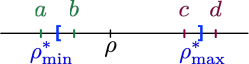
Figure 1: Relationship between the binary search intervals $[a,b]$ and $[c,d]$ and the true interval $[\rho_{\rm min}^{*},\rho_{\rm max}^{*}]$ on which $\mathcal{A}(x,\rho^{\prime})$ outputs $y_{\rho}$.

C.2 Learning a Metric and Interpolating Between Single and Complete Linkage

Finally, we consider an extension of the clustering algorithm family introduced in Section 4.2 that allows us to also learn the best metric to use for a specific clustering domain. We suppose that the clustering domain is equipped with two base metrics and our goal is to learn the best convex combination of them. For example, one metric could be based on a neural network feature embedding and the other could be a hand-designed metric based on domain expertise. Formally, each clustering instance is described by a pair of distance matrices $D_{0}$ and $D_{1}$ specifying the distances between each pair of points according to the two metrics.

The algorithm family we consider called $\rho$-metric-linkage has two parameters, $\rho\in[0,1]$ which is used to interpolate between single and complete linkage as in Section 4.2, and $\alpha\in[0,1]$, which is used to interpolate between the two distance metrics. In particular, for any $\alpha\in[0,1]$, let $D_{\alpha}=(1-\alpha)D_{0}+\alpha D_{1}$ and denote its entries by $(d_{\alpha,i,j})$. The algorithm with parameters $\rho$ and $\alpha$ repeatedly merges the pair of clusters $A$ and $B$ that are closest according to the distance $d_{\rho,\alpha}(A,B)=(1-\rho)\min_{a\in A,b\in B}d_{\alpha,a,b}+\rho\max_{a\in A,b\in B}d_{\alpha,a,b}$.

We provide dispersion analysis for this algorithm family under the assumption that both distance matrices for each problem instance are $\kappa$-smooth, meaning that their entries are independent and each have $\kappa$-bounded discontinuities.

Theorem 21.

Consider an adversary choosing clustering instances where the $t^{\rm th}$ instance has two symmetric distance matrices $D^{(t)}_{0},D^{(t)}_{1}\in[0,B]^{n\times n}$ and for all $i<j$, the $(i,j)^{\text{th}}$ entry of $D^{(t)}_{0}$ and $D^{(t)}_{1}$ are $\kappa$-smooth. The loss functions $\ell_{1},\ell_{2},\dots$ defined above are piecweise constant and $f$-dispersed for $f(T,\epsilon)=O(Tn^{8}\kappa^{3}\epsilon+\sqrt{T\log(Tn)})$ and $\beta$-dispersed for $\beta=1/2$.

Proof sketch..

First, we argue that for any pair of distance matrices $D_{0}$ and $D_{1}$, we can partition the $\alpha$-parameter space into $O(n^{4})$ regions such that on each region the ordering over pairs of points $(i,j)$ according to the distance $d_{\alpha,i,j}$ is fixed. In particular, on each region, the closest and farthest pair of points between any pair of clusters are constant. Next, restricted to each of these regions, we find that we can express the distance $d_{\rho,\alpha}(A,B)$ between any pair of clusters as a quadratic function of the parameters $\rho$ and $\alpha$. This implies that for any pair of candidate merges $(A,B)$ and $(A^{\prime},B^{\prime})$, the algorithm prefers to merge $(A,B)$ over $(A^{\prime},B^{\prime})$ whenever the quadratic polynomial $q_{A,B,A^{\prime},B^{\prime}}(\rho,\alpha)=d_{\rho,\alpha}(A,B)-d_{\rho,\alpha}(A^{\prime},B^{\prime})$ is negative. While there are exponentially many choices of the $4$ clusters, the coefficients of this quadratic depend on the distances between a set of $8$ points, and therefore there are only $O(n^{8})$ unique quadratic functions. Next, we argue that for any fixed $\alpha$, the polynomial $\rho\mapsto q_{A,B,A^{\prime},B^{\prime}}(\rho,\alpha)$ has coefficients with joint density bounded by $O(\kappa^{3})$ and whose magnitude are bounded by $O(B)$ (and similarly for fixing any $\rho$ and treating the polynomial as a function of $\alpha$ alone). Now consider any pair of parameters $(\rho,\alpha)$ and $(\rho^{\prime},\alpha^{\prime})$ that are within distance $\epsilon$. The piecewise-linear path given by the line segment from $(\rho,\alpha)$ to $(\rho,\alpha^{\prime})$ followed by the line segment $(\rho,\alpha^{\prime})$ to $(\rho^{\prime},\alpha^{\prime})$ has total length $O(\epsilon)$. The above arguments combined with Theorem 6 ensures that this path contains a root of the quadratic $q_{A,B,A^{\prime},B^{\prime}}$ with probability at most $O(\kappa^{3}\epsilon)$. Therefore, the expected number of discontinuities intersecting the rectilinear path between any pair of paremeter vectors at distance $\epsilon$ is upper bounded by $O(Tn^{8}\kappa^{3}\epsilon)$ (by summing over the $O(n^{8})$ different quadratics obtained from each of the $T$ instances). Applying Theorem 9 we are guaranteed that the worst rectilinear path has at most $\tilde{O}(Tn^{8}\kappa^{3}\epsilon+\sqrt{T})$ discontinuities, which proves the claim. ∎

Appendix D Transformations of Bounded Densities

In this section we summarize several useful results that provide upper bounds on the density of random variables that are obtained as functions of other random variables with bounded density functions. These results allow us to reason about the distribution of discontinuity locations that arise as transformations of random problem parameters in algorithm configuration instances.

In many cases, we make use of the following result:

Theorem 22 (Density Function Change of Variables).

Let $X\in\mathbb{R}^{d}$ be a random vector with joint probability density function $f_{X}:\mathbb{R}^{d}\to[0,\infty)$ and let $\phi:\mathbb{R}^{d}\to\mathbb{R}^{n}$ be any bijective differentiable function. Then the random vector $Y=\phi(X)$ also has a density function $f_{Y}:\mathbb{R}^{n}\to[0,\infty)$ given by $f_{Y}(y)=|\det(J_{\phi^{-1}}(y))|f_{X}(\phi^{-1}(y))$, where $J_{\phi^{-1}}(y)$ denotes the Jacobian of $\phi^{-1}$ evaluated at $y$.

Lemma 23 (Lemma 6 from [11]).

Suppose $X$ and $Y$ are random variables taking values in $(0,1]$ and suppose that their joint distribution is $\kappa$-bounded. Then the distribution of $Z=\ln(X/Y)$ is $\kappa/2$-bounded.

Lemma 24 (Lemma 8 from [11]).

Suppose $X$ is a random variable with a $\kappa$-bounded density and suppose $c$ is a constant. Then $Z=X/c$ has a $c\kappa$-bounded density

Lemma 25.

Let $X$ and $Y$ be two independent random variables each having densities upper bounded by $\kappa$. The random variable $U=X+Y$ has density $f_{U}$ satisfying $f_{U}(u)\leq\kappa$ for all $u$.

Proof.

Let $f_{X}$ and $f_{Y}$ be the density functions for $X$ and $Y$, respectively. The density for $U$ is the convolution of $f_{X}$ and $f_{Y}$. With this, we have

$$f_{U}(u)=\int_{-\infty}^{\infty}f_{X}(u-y)f_{Y}(y)\,dy\leq\int_{-\infty}^{\infty}\kappa f_{Y}(y)\,dy=\kappa.$$

It follows that $U=X+Y$ has a density that is upper bounded by $\kappa$. ∎

Lemma 26.

Let $X$ and $Y$ be random variables with joint density $f_{XY}$ that is $\kappa$-bounded and such that $|Y|\leq M$ with probability 1 and let $U=X/Y$. Then the density function $f_{U}$ is $\kappa M^{2}$-bounded.

Proof.

Consider the change of variables given by $U=X/Y$ and $V=Y$. This corresponds to the transformation function $\phi(x,y)=(x/y,y)$. The inverse of $\phi$ is given by $\phi^{-1}(u,v)=(uv,v)$. The Jacobian of $\phi^{-1}$ is

$$J_{\phi^{-1}}(u,v)=\left[\begin{matrix}v&u\\ 0&1\end{matrix}\right],$$

whose determinant is always equal to $v$. Therefore, the joint density of $U$ and $V$ is given by

$$f_{UV}(u,v)=|v|f_{XY}(uv,v).$$

To get the marginal density for $U$, we integrate over $v$ and use the fact that the density $f_{XY}(x,y)=0$ whenever $|y|>M$. This gives

$$f_{U}(u)=\int_{-M}^{M}|v|f_{XY}(uv,v)\,dv\leq\kappa\int_{-M}^{M}|v|\,dv=\kappa M^{2}.$$

It follows that the density for $U$ satisfies $f_{U}(u)\leq\kappa M^{2}$ for all $u$, as required. ∎

Lemma 27.

Let $X$ and $Y$ be independent random variables with $\kappa$-bounded densities so that $|X|\leq M$ and $|Y|\leq M$ with probability one and define $Z=X/(X+Y)$. The random variable $Z$ has a density function $f_{Z}$ that is $4\kappa^{2}M^{2}$-bounded.

Proof.

Consider the change of variables given by $U=X$ and $V=X+Y$. We will argue that the joint density $f_{UV}$ is $\kappa^{2}$-bounded. Then, since $|X+Y|\leq 2M$ with probability 1, we can apply Lemma 26 to ensure that the density of $Z=U/V$ is bounded by $\kappa^{2}(2M)^{2}=4\kappa^{2}M^{2}$, as required.

It remains to bound the joint density of $U=X$ and $V=X+Y$. This change of variables corresponds to the transformation function $\phi(x,y)=(x,x+y)$, whose inverse is given by $\phi^{-1}(u,v)=(u,v-u)$. The Jacobian of $\phi^{-1}$ is given by

$$J_{\phi^{-1}}(u,v)=\left[\begin{matrix}1&0\\ -1&1\\ \end{matrix}\right],$$

whose determinant is always $1$. It follows that the joint density for $(U,V)$ is given by $f_{UV}(u,v)=f_{XY}(u,v-u)=f_{X}(u)f_{Y}(v-u)\leq\kappa^{2}$, as required. ∎

Lemma 28.

Let $X$, $Y$, and $Z$ be independent random variables with $\kappa$-bounded densities such that $|Y|\leq M$, and $|Z|\leq M$ with probability one. Then the random variable $R=\frac{X+Y}{Z+Y}$ has a density $f_{R}$ that satisfies $f_{R}(u)\leq 4\kappa^{2}M^{2}$.

Proof.

Consider the change of variables given by $U=X+Y$, $V=Z+Y$. We will argue that the joint density $f_{UV}$ for $U$ and $V$ is $\kappa^{2}$-bounded. Then, since $|V|=|Z+Y|\leq 2M$ with probability 1, we can apply Lemma 26 to ensure that the density of $R=U/V$ is bounded by $4\kappa^{2}M^{2}$, as required.

It remains to bound the joint density of $U=X+Y$ and $V=Z+Y$. Consider the change of variables given by $U=X+Y$, $V=Z+Y$, and $W=Y$. This corresponds to the transformation function $\phi(x,y,z)=(x+y,z+y,y)$, and has inverse $\phi^{-1}(u,v,w)=(u-w,w,v-w)$. The Jacobian of $\phi^{-1}$ is given by

$$J_{\phi^{-1}}(u,v,w)=\left[\begin{matrix}1&0&-1\\ 0&0&1\\ 0&1&-1\end{matrix}\right],$$

which always has determinant given by $-1$. It follows that the joint density for $(U,V,W)$ is given by

$$f_{UVW}(u,v,w) =f_{XYZ}(u-w,w,v-w)$$

$$=f_{X}(u-w)f_{Y}(w)f_{Z}(v-w).$$

To get the joint density over only $U$ and $V$ we integrate over $w$:

$$f_{UV}(u,v) =\int_{-\infty}^{\infty}f_{X}(u-w)f_{Y}(w)f_{Z}(v-w)\,dw$$

$$\leq\kappa^{2}\int_{-\infty}^{\infty}f_{Y}(w)\,dw$$

$$=\kappa^{2},$$

as required. ∎

References

- Aamand et al. [2019] Anders Aamand, Piotr Indyk, and Ali Vakilian. (learned) frequency estimation algorithms under zipfian distribution, 2019.
- [2] Noga Alon, Nicolò Cesa-Bianchi, Claudio Gentile, Shie Mannor, Yishay Mansour, and Ohad Shamir. Nonstochastic multi-armed bandits with graph-structured feedback. SIAM J. Comput.
- Audibert et al. [2014] Jean-Yves Audibert, Sébastien Bubeck, and Gábor Lugosi. Regret in online combinatorial optimization. Mathematics of Operations Research, 2014.
- Auer et al. [2002] Peter Auer, Nicolo Cesa-Bianchi, Yoav Freund, and Robert E Schapire. The nonstochastic multiarmed bandit problem. SIAM journal on computing, 2002.
- Awasthi et al. [2012] Pranjal Awasthi, Avrim Blum, and Or Sheffet. Center-based clustering under perturbation stability. In Information Processing Letters, 2012.
- Awasthi et al. [2014] Pranjal Awasthi, Maria-Florina Balcan, and Konstantin Voevodski. Local algorithms for interactive clustering. In ICML, 2014.
- Balcan and Liang [2016] Maria-Florina Balcan and Yingyu Liang. Clustering under perturbation resilience. In SIAM Journal on Computing, 2016.
- Balcan et al. [2016] Maria-Florina Balcan, Nika Haghtalab, and Colin White. -center clustering under perturbation resilience. In ICALP, 2016.
- Balcan et al. [2017] Maria-Florina Balcan, Vaishnavh Nagarajan, Ellen Vitercik, and Colin White. Learning-theoretic foundations of algorithm configuration for combinatorial partitioning problems. COLT, 2017.
- Balcan et al. [2018a] Maria-Florina Balcan, Travis Dick, Tuomas Sandholm, and Ellen Vitercik. Learning to branch. In ICML, 2018a.
- Balcan et al. [2018b] Maria-Florina Balcan, Travis Dick, and Ellen Vitercik. Dispersion for data-driven algorithm design, online learning, and private optimization. In FOCS, 2018b.
- Balcan et al. [2018c] Maria-Florina Balcan, Travis Dick, and Colin White. Data-driven clustering via parameterized lloyd’s families. In NeurIPS, 2018c.
- Balcan et al. [2018d] Maria-Florina Balcan, Tuomas Sandholm, and Ellen Vitercik. A general theory of sample complexity for multi-item profit maximization. In EC, 2018d.
- Ben-David et al. [2009] Shai Ben-David, David Pal, and Shai Shalev-Shwartz. Agnostic online learning. In COLT, 2009.
- Caseau et al. [1999] Yves Caseau, François Laburthe, and Glenn Silverstein. A meta-heuristic factory for vehicle routing problems. In International Conference on Principles and Practice of Constraint Programming, 1999.
- Cohen-Addad and Kanade [2017] Vincent Cohen-Addad and Varun Kanade. Online Optimization of Smoothed Piecewise Constant Functions. In AISTATS, 2017.
- Demmel et al. [2005a] Jim Demmel, Jack Dongarra, Victor Eijkhout, Erika Fuentes, Antoine Petitet, Rich Vuduc, R Clint Whaley, and Katherine Yelick. Self-adapting linear algebra algorithms and software. Proceedings of the IEEE, 2005a.
- Demmel et al. [2005b] Jim Demmel, Jack Dongarra, Victor Eijkhout, Erika Fuentes, Antoine Petitet, Rich Vuduc, R Clint Whaley, and Katherine Yelick. Self-adapting linear algebra algorithms and software. Proceedings of the IEEE, 2005b.
- Dong et al. [2019] Yihe Dong, Piotr Indyk, Ilya Razenshteyn, and Tal Wagner. Learning space partitions for nearest neighbor search, 2019.
- Grosswendt and Roeglin [2015] Anna Grosswendt and Heiko Roeglin. Improved analysis of complete linkage clustering. In European Symposium of Algorithms, 2015.