Performance of the Gemini Planet Imager Non-Redundant Mask and spectroscopy of two close-separation binaries HR 2690 and HD 142527

Abstract

The Gemini Planet Imager (GPI) contains a 10-hole non-redundant mask (NRM), enabling interferometric resolution in complement to its coronagraphic capabilities. The NRM operates both in spectroscopic (integral field spectrograph, henceforth IFS) and polarimetric configurations. NRM observations were taken between 2013 and 2016 to characterize its performance. Most observations were taken in spectroscopic mode with the goal of obtaining precise astrometry and spectroscopy of faint companions to bright stars. We find a clear correlation between residual wavefront error measured by the AO system and the contrast sensitivity by comparing phase errors in observations of the same source, taken on different dates. We find a typical 5-$\sigma$ contrast sensitivity of $2-3~{}\times~{}10^{-3}$ at $\sim\lambda/D$. We explore the accuracy of spectral extraction of secondary components of binary systems by recovering the signal from a simulated source injected into several datasets. We outline data reduction procedures unique to GPI’s IFS and describe a newly public data pipeline used for the presented analyses. We demonstrate recovery of astrometry and spectroscopy of two known companions to HR 2690 and HD 142527. NRM+polarimetry observations achieve differential visibility precision of $\sigma\sim 0.4\%$ in the best case. We discuss its limitations on Gemini-S/GPI for resolving inner regions of protoplanetary disks and prospects for future upgrades. We summarize lessons learned in observing with NRM in spectroscopic and polarimetric modes.

1 Introduction

Exoplanet imaging survey instruments reach deep contrast performance by attenuating the stellar PSF using a coronagraph (e.g. Oppenheimer et al., 2012; Macintosh et al., 2014; Beuzit et al., 2008; Liu et al., 2010). Many designs have significantly reduced sensitivity within a $5~{}\lambda/D$ angular region around the host star, where $\lambda$ is the wavelength and $D$ is the telescope diameter. High resolution, non-occulting methods, like non-redundant mask (NRM) interferometry (e.g., Baldwin et al., 1986; Tuthill et al., 2000), complement high contrast methods by probing small spatial scales at moderate contrast. NRM coupled with adaptive optics can reach contrast of about 6 magnitudes at $\lambda/B$, with reduced contrast below $\lambda/B$ (Lacour et al., 2011). In this case $B$ is the longest baseline spanned by the mask (typically close to the telescope diameter). This complementary high resolution approach can reveal the presence of close-in structures to bright point sources, particularly exciting for young protoplanetary systems. The NRM is especially suited for multiplicity studies at $<2\lambda/D$ scales. Combined with polarimetry, resolved polarized structures can be resolved close in to the host star.

High resolution imaging can play an important role in bridging the gap between companion point source detection methods. Very high contrast methods probe the outer architectures of solar systems and have little or no overlap with astrometry or radial velocity detection sensitivities (the latter in part due to differences in age sensitivities between RV and imaging). High resolution methods like NRM are sensitive to a objects at intermediate separations, especially for sources over $100$pc away. NRM on large ground-based telescopes has been used to resolve structure in the gaps of transitional disks (e.g., Kraus & Ireland, 2012; Biller et al., 2012; Sallum et al., 2015a), has helped push multiplicity studies to closer separations (e.g. Kraus et al., 2008; Sana et al., 2014; Duchêne et al., 2018) and track the orbits of close binaries in combination with radial velocity to determine dynamical masses for young stellar binaries (Rizzuto et al., 2016). NRM has also been used for image reconstruction of massive stars (e.g., Tuthill et al., 1999; Norris et al., 2012a) and disks (e.g., Cheetham et al., 2015; Sallum et al., 2015b).

Combining aperture masking with an adaptive optics (AO) system provides stable observations to take advantage of both image quality provided by AO and self-calibrating observables measured with a non-redundant pupil. By splitting the pupil into a set of unique hole-to-hole baseline pairs, fringe phases and amplitudes can be measured uniquely, where each fringe is formed from a pupil baseline. In addition, phase closure calibrates hole-based phase errors that arise from atmospheric fluctuations and instrument non-common path aberrations (Jennison, 1958). In the case of extreme adaptive optics (ex-AO), which uses thousands of actuators to correct small corrugations in the wavefront, interference fringes are stable over many seconds of integration making fainter sources more accessible through this method.

In this paper we present results from observations with the Gemini Planet Imager NRM and discuss the performance and post-processing in detail. Our analysis provides a comparison with aperture masking on other ground-based instruments, and demonstrate complementarity with upcoming space-based NRM on JWST-NIRISS (Doyon et al., 2012). We confirm results using two different data pipelines detailing the data reduction procedures. With the release of this article, we make our primary pipeline public, along with examples of analyses in this paper.

2 Implementing NRM on The Gemini Planet Imager

2.1 The Gemini Planet Imager’s non-redundant mask

GPI has a 10-hole non-redundant mask (Fig. 1) in its apodizer wheel, a warm pupil located after the deformable mirror. We provide the mask hole coordinates with respect to the primary mirror in Table 1, including the outer diameter physical size in the apodizer wheel where the mask sits. This pupil mask transmits roughly 6.2% of the light compared to a completely unocculted pupil (not considering spiders, secondary obstructions, or Lyot stops). The mask forms 45 unique baselines (spatial frequencies), which correspond to 45 fringes in the image plane. $\lambda/B$ spans $\sim 45-330$ mas in H band. There are 120 total combinations of hole triplets that form closing triangles, and a set of 36 unique triangles that don’t repeat any baseline.

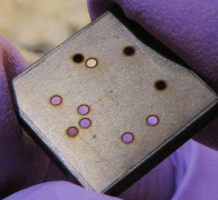
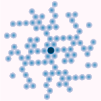
Figure 1: Left: The 10-hole non-redundant mask on the Gemini Planet Imager. Right: Associated spatial frequency coverage, where the longest baseline is $6.68~{}$m.

Table 1: Mask hole dimensions measured in mm from center.

X	Y
-1.061	-3.882
-0.389	-5.192
2.814	-0.243
3.616	0.995
-4.419	2.676
-1.342	5.077
-4.672	-2.421
4.157	-2.864
5.091	0.920
1.599	4.929

Hole diameter: 0.920 mm
Gemini S outer diameter (OD): 7.770 m (after baffling)
Apodizer outer diameter in this re-imaged pupil plane: 11.68 mm. (Lenox Laser, Glen Arm, MD).
Projection of in-pupil coordinates are magnified by a factor of $\sim 650$ onto the primary.

GPI’s focal plane masks are implemented as mirrors that reflect the off-axis light to the science channel and pass the on-axis starlight through a central hole. In NRM mode, we use a mirror with no hole, so the full field of view passes to the IFS. However, in coronagraph mode the central starlight is sent to a tip/tilt sensor for additional low-order correction. Therefore, all non-coronagraphic observations do not benefit from this additional tip/tilt correction. Small jitter in the image leads to slight smearing of fringes and reduced contrast. This is worsened in poorer weather conditions, including high winds. We discuss this in detail in Section 4.3.

The NRM pupil position for GPI has been measured and fixed to lie entirely within the pupil and not overlap with any defective actuators or spider supports. The in-pupil mask coordinates are listed in Table 1 and are converted to projected coordinates on the primary mirror by the factor between the pupil and primary outer diameter (OD): $7770.1/11.998$. The position should not need to be adjusted but any vignetting can be investigated with the pupil-viewing camera. A detailed discussion of the procedure to determine the mask orientation and adjusting its position can be found in Greenbaum et al. (2014). Baseline coordinates are computed as $U_{i,j}=X_{i}-X_{j}$,$V_{i,j}=Y_{i}-Y_{j}$ for $[i,j]$ combinations, where $X$ and $Y$ are the mask hole position in the pupil (Table 1). In the coordinate system used in this work, to reach the detector orientation the mask coordinates were rotated clockwise by $114.7^{\circ}$. In Python, Converting the initial baseline vectors $[U_{0},V_{0}]$ into vectors rotated by $\theta$, $[U_{r},V_{r}]$ consists of the operation: $U_{r}=U_{0}\cos(\theta)-V_{0}\sin(\theta)$, $V_{r}=U_{0}\sin(\theta)+V_{0}\cos(\theta)$.

2.2 Observing Sequences and Calibration

Uncorrected wavefront and non-common path errors lead to residual phase errors. At least one nearby calibration source, close in time, (single, unresolved) should be observed in a sequence. In spectroscopic mode it is less important to choose a calibration source that matches the target color because the individual wavelength slices are close to monochromatic. A calibration source should aim to match the target brightness in the wavefront sensing filter (approximately I band). Multiple calibration sources in a survey-like program can provide a good estimate of systematic calibration errors (e.g., Kraus et al., 2008), as long as the sources are observed consecutively, in similar conditions. However, in the case of observing individual science targets it may not be practical or efficient to obtain many calibration sources.

At current operation, it takes approximately 10 minutes to slew to and acquire a new target. This makes back and forth switching between target and calibration source time consuming. We have adopted the strategy of observing the target in full sequence followed by one or two calibration sources. A polarimetric sequence additionally involves looping through four half waveplate angles (HWPAs) per “integration.” While this increases the total integration on source compared to the spectroscopic mode, polarimetric images are broadband so each integration is generally shorter.

Choosing the exposure time for a single integration is a balance between observation efficiency and minimizing fringe smearing. Typically, we aim for an exposure time that provides at minimum $3000$ counts in the peak of the raw detector image and at maximum $14000$ counts to avoid saturation. The total number of photons collected should satisfy the desired contrast sensitivity. We discuss systematics that degrade contrast sensitivity beyond photon noise in Section 4.3.

Table 2 lists the approximate maximum brightness for NRM observations in each filter combination. All brightness limits and estimated exposure times approximate and derived empirically from commissioning observations. An empirically-determined exposure time calculator is available in the ImPlaneIA pipeline.

Table 2: Gemini Planet Imager approximate maximum brightness limits for all NRM settings. All values are in apparent magnitude in the specified band.

MODE	Y	J	H	K1	K2
Spectroscopic	1.8	2.2	1.8	1.8	1.8
Polarimetric	3.0	3.0	3.0	3.0	3.0

3 Observations and data reduction

All observations discussed in this paper were taken on the Gemini Planet Imager with its 10-hole non-redundant mask, as a part of program GS-ENG-GPI-COM. A summary of the observations, all taken in stationary pupil mode, is contained in Table 3. The observations presented in this paper focus mostly on point sources in a range of conditions to determine contrast limits and polarization precision, as well as two binary systems at different contrast ratios.

Table 3: Summary of observations presented in this paper, indicating date string, source name, observing mode, total integration time, and various observatory parameters. All observations are taken in stationary pupil mode so that the sky rotates with respect to the detector.

Date	Source	Mode	Single	$N_{exp}$	$=$ Total	Seeing	WFE	Airmass	Wind	sky rot
YYMMDD			[s]		[s]	($\arcsec$)	[nm]		[m/s]	[deg]
131211	HR 2690	NRM Spect - H	59.6	8	476.8	0.67	116.15	1.23	0.49	0.021
	HR 2716	NRM Spect - H	59.6	8	476.8	0.58	121.80	1.23	0.36	0.37
	HR 2839	NRM Spect - H	43.6	8	348.8	0.51	134.2	1.23	0.40	0.234
140324	HD 63852	NRM Spect - H	1.5	20	30.0	0.87	81.99	1.17	0.41	0.67
140511	HD 63852	NRM Spect - H	1.5	20	30.0	0.81	160.94	1.55	11.5	0.5
	Internal	NRM Spect - H	1.5	63	94.5	N/A	32.82	N/A	N/A	N/A
140512	HD 142527	NRM Spect - J	59.6	9	536.4	1.4	190.57	1.03	8.5	11.4
	HD 142695	NRM Spect - J	53.8	8	430.4	1.4	177.77	1.04	8.6	5.0
160504	HIP 74604	NRM pol - K1	4.4	40	176.0	2.19	144.23	1.08	4.6	1.5

During commissioning in December of 2013 we observed the known binary HR 2690 ($\Delta H\sim 2$) and two unresolved calibration sources HR 2716 and HR 2839. This sequence of observations was chosen to demonstrate the recovery of a moderate contrast binary system for proof of concept. In March of 2014 we observed bright single source HD 63852 to estimate contrast limits compared to the ideal case of the internal source. In May of 2014 we returned to this source, providing a comparison between observing epochs. We also observed HD 142527, which contains an M-dwarf companion, HD 142527 B ($\Delta J\sim 4.6$) to demonstrate deeper contrast retrieval of a known binary companion. For this dataset we observed two calibration sources HD 142695 and HD 142384, though the latter was found to be a close binary after our observations (Le Bouquin, 2014). Details of the analysis are in §4. In May of 2016 we took polarimetric observations of bright unresolved sources to determine calibration limit and assess systematic biases. We present one example, HIP 74604, our best dataset, and discuss polarimetric sensitivity in §5.

3.1 Raw data reduction

The data are processed from raw 2D detector exposures into datacubes of images at each wavelength or polarization through the GPI Data Reduction Pipeline (DRP) (Perrin et al., 2014). Wavelength calibration is performed with Argon arc lamp exposures. Shifts in the location of the spectra due to flexure are calibrated by arc lamp exposures taken close in time to each set of observations Wolff et al. (2014). For polarimatry data we use the recipe template for polarization data taken with the NRM called “Basic NRM Polarization Datacube Extraction,” which performs the polarimetric spot calibration, smooths polarization calibration, subtracts a dark background, corrects for 2D flexure, removes microphonics noise, and interpolates bad pixels in the raw frame before assembling the polarization data cube. Details of DRP primitives can be found in online documentation.

3.2 Extracting Fringe observables

We measure fringe phases and amplitudes from reduced datacubes using two different aperture masking pipelines, the Sydney University pipeline, based in IDL, and a pipeline implementing the Lacour-Greenbaum (LG) algorithm (Greenbaum et al., 2015), based in Python. The former analyzes images in the Fourier domain. The latter measures fringes in the image plane.

The Fourier plane approach used in the Sydney pipeline measures the phases and square-visibilities directly from the Fourier transform of the image. First, images are multiplied by a super-Gaussian window function of the form $e^{-kx^{4}}$, which has the effect of smoothing in the Fourier plane. Then, images are Fourier transformed, which separates the information from different baselines into distinct regions. The phases and visibilities are measured for all points in a 3-Fourier sampling element radius around the predicted frequency for each baseline. To calculate the square-visibilities and phases for each baseline, these measurements are combined by weighting with a matched filter. Closure phases are formed by considering sets of 3 baselines that form a closing triangle (i.e. the vector sum of their frequencies is zero). Rather than use the weighted phases for each baseline, instead a number of measurements are calculated from each set of 3 pixels (within a small area around the predicted frequency of each baseline) that forms a closing triangle. These are then combined by weighting with a matched filter (e.g. Monnier, 1999). This matched filter approach relies on pre-computing the expected Fourier-plane profile of NRM images using fixed values for the size of the pupil mask holes, plate scale and wavelength for each IFS channel.

The image plane pipeline assumes a plate scale and monochromatic wavelength (spectroscopic mode) or defined bandpass (polarimetric/broadband mode) and fits $A^{\prime}\sin(k\cdot\Delta x_{i,j})+B^{\prime}\cos(k\cdot\Delta x_{i,j})$ to each fringe generated by particular hole-pair baselines, where $A^{\prime}=A\sin(\Delta\phi)$ and $B^{\prime}=B\cos(\Delta\phi)$, $\phi$ is the fringe phase shift, and $\sqrt{A^{2}+B^{2}}$ is the fringe amplitude. Here, $k=(u,v)$ is the 2D coordinate in the image plane. This algorithm is described in detail in §3 of Greenbaum et al. (2015). The sub-pixel centering of the image is measured by computing $x$ and $y$ tilt in the numerical Fourier transform of the image. This centroid is used to sample the model onto oversampled detector pixels, which are then binned to the detector scale. For NRM+polarimetry (or broadband) images, for which there is dispersion in the PSF we use filter transmission files available in the GPI DRP and an approximate source spectrum to model the dispersion.

We compared the two pipelines and confirmed that they yield consistent results. We show results from the image-plane pipeline in this paper. An image-plane pipeline using the LG algorithm, ImPlaneIA (Greenbaum et al., 2018; Greenbaum, 2018) is available publicly with further documentation and examples.

3.3 Calibration and analysis of fringe observables

Both the Sydney and LG pipelines use similar analysis tools following calculation of fringe observables to produce the results shown in this paper.

For spectroscopic data we compute an average closure phase and standard error over the set of integrations for each baseline (each mask hole pair for each wavelength slice). This produces $N_{\mathrm{triangles}}\times N_{\lambda}$ observables. In this case $N_{\mathrm{triangles}}=120$ in one datacube slice, and $N_{\lambda}=37$. In general, we do not see a large amount of field rotation in our observation sequences (see Table 3) so we compute an average position and consider an average parallactic angle. For our observations of HD 142527, which contains $\sim 11^{\circ}$ of rotation, we compared the results when accounting for sky rotation by splitting exposures into smaller groups (see §4 for more details). We subtract measured average closure phases from the calibration source(s) from our science target closure phases and add errors in quadrature.

Binary detection and contrast limits rely on a model for the fringe visibility of a binary point source:

$$V_{u,v}=\frac{1+re^{-2\pi i(\alpha\cdot u+\delta\cdot v)}}{1+r}$$ (1)

where $r$ is the contrast ratio between the secondary and primary, $u,v$ are the baseline coordinates a given hole pair, and $\alpha,\delta$ are the sky coordinates of the secondary relative to the primary. The absolute orientation is calibrated in the standard way for GPI data, accounting for the orientation of the lenslet array ($+23.5^{\circ}$), detector, and instrument position angle (PA). Plate scale and PA calibrations have been performed by the observation of astrometric calibrators yielding a pixel scale of $14.166\pm 0.007$ and a north offset of $-0.1^{\circ}\pm 0.13$ (Konopacky et al., 2014; De Rosa et al., 2015). The derotation angle in degrees to place North up is $\mathrm{AVPARANG}-\mathrm{AVCASSANG}+23.4$. AVPARANG and AVCASSANG are header keywords in GPI data files.

In practice closure phase errors are often underestimated from the data, especially when only one or two calibration sources are observed and systematic errors cannot be properly determined. We scale the errors by a factor $\sqrt{N_{holes}/3}$ to account for redundancy from repeating baselines. Additionally, we add additional constant error to the closure phases so that the reduced $\chi^{2}$ is close to 1.

The binary detection limits reported in this paper are estimated from the calibrated closure phase errors based on a signal-to-noise ratio (SNR) threshold, where

$$SNR = \sqrt{\sum_{i=1}^{N_{CP}}CP_{i,\alpha,\delta,r}^{2}/\sigma_{i,CP}^{2}}$$ (2)

Model closure phases are calculated from equation 1. Model phases scale roughly linearly with contrast ratio $r$. We estimate contrast ratio detection limit at SNR=5 as:

$$r_{5}=\frac{5\times r_{model}}{SNR}$$ (3)

To generate contrast curves we compute $r_{5}$ over a range of separations and position angles. Sensitivity varies somewhat with position angle based on mask geometry. GPI’s mask has fairly uniform visibility coverage, improved further in spectroscopic mode by the wavelength axis.

In polarimetric mode, the light is split with a Wollaston prism into two orthogonal polarizations. A half-wave plate optic is used to rotate the angle of polarization during observation (Perrin et al., 2015). This enables a differential measurement between orthogonal polarizations for both fringe amplitude and fringe phase. We compute differential visibilities and differential closure phases following Norris et al. (2015).

With 4 half-wave plate (HWP) rotations at 0, 22.5, 45, and 67.5 degrees, we can build up two layers of calibration. First we calibrate orthogonal polarizations in a single image:

$$CP_{ortho-diff} = CP_{channel1}-CP_{channel2}$$

$$V_{ortho-diff} = \frac{V_{channel1}}{V_{channel2}}$$ (4)

Next we calibrate orthogonal HWP rotations, for example, HWPA=$0^{o}$ with HWPA=$45^{o}$:

$$CP_{0-45} = CP_{diff-0}-CP_{diff-45}$$

$$V_{0-45} = \frac{V_{diff-0}}{V_{diff-45}}$$ (5)

This should remove instrumental effects, which would contribute to all polarization states.

4 Spectroscopic mode & binary contrast performance

The spectroscopic mode on GPI provides a nearly monochromatic image at a set of wavelengths across each filter. Lack of bandwidth smearing makes fringe extraction straightforward in this configuration. The extra wavelength dimension provides many more baselines for a single observation, $N_{\lambda}\times N_{baselines}$ compared to $N_{baselines}$, where $N_{\lambda}$ is typically 37 for GPI.

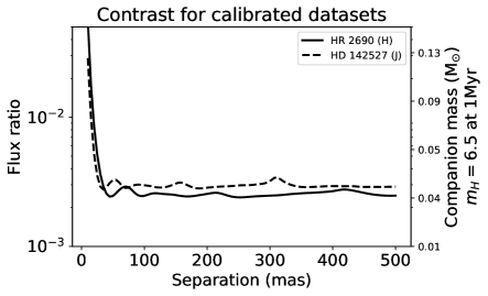
Figure 2: Contrast limits at SNR=5 for the two spectroscopic mode calibrated datasets analyzed in this paper, for HR 2690 ($\sim 8$ minutes in H band) and HD 142527 ($\sim 9$ minutes in J band). The righthand vertical axis shows the corresponding companion mass for given an apparent H magnitude of 6.5 for the primary assuming an age of 1Myr at 140pc using the AMES-Cond models (Baraffe et al., 2003).

Zimmerman et al. (2012) demonstrated improved contrast from the set of IFS+NRM images compared to the combined dataset using the P1640 IFS. We find similar results when we analyze phase errors measured over all wavelength channels of the full datacube compared to data collapsed over the wavelength axis. For the collapsed data we model the PSF as polychromatic considering the approximate H-band filter throughput profile for GPI. The rest of the analysis is identical to the typical GPI case described in §3.2.

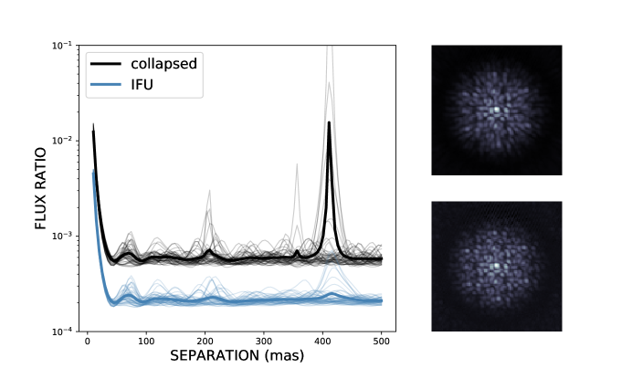
Figure 3: Performance comparison based on internal source data for $\lambda$-collapsed (black) and IFS data (blue). The contrast is estimated at SNR=5. The first half of the data are calibrated with the second half, overestimating performance. The right panel shows snapshots of the data. The IFS provides twice the sensitivity and smooths out low-sensitivity windows at 200 and 400 mas.

In Figure 3 we show an estimated contrast curve for an example dataset taken with the GPI internal source in the light blue curves, which uses all wavelength channels. The contrast curve is computed according to Equations 2 and 3 after scaling the errors by the baseline redundancy. We also scale the errors by a factor $\sqrt{37/17}$, which roughly accounts for the fact that we measure $37$ wavelength channels interpolated over about 17 pixels. The full set of datacubes are split into two halves of exposures and calibrated against each other. This likely overestimates the sensitivty, but we consider the relative performance between data taken in different observing conditions. When the data is summed into one polychromatic image, contrast sensitivity is a factor of $\sim 2-3$ worse. The spectroscopic mode is ideal for detection of faint companions to bright host stars, providing increased signal to noise overall. The additional spatial frequency coverage reduces regions of very low sensitivity that arise from the baseline configuration (i.e. the peak of the collapsed cube curve at $\sim 200$ and $\sim 400$ mas).

4.1 Analyzing IFS Data - Simulation Example

Spectral mode datasets can provide robust binary detection, constraining a companion’s position at multiple wavelengths. We explore errors and biases on parameter estimation with simulated data of a binary source. The data are simulated from shifting and adding point source images measured from GPI’s internal light source. Using internal source data ensures there is no resolved structure in the primary and also that the data still represent aspects of the GPI PSF that are not modeled (e.g., vibrations, detector effects). In general, this example will underestimate typical errors for two reasons: the bright internal source PSF is much more stable and the secondary companion is simulated from the same data as the PSF calibrator (as though one had a “perfect” calibrator). We use this as an example to demonstrate the approach and provide more practical examples in §4.4 and §4.5. The simulated faint companion 45.5 mas away ($\sim 1.2\lambda/D$, $\sim 1.0\lambda/B_{max}$) at a position angle of 18.4^∘. We simulate an example flux ratio spectrum between two Phoenix models (e.g., Allard et al., 2003) at $\mathrm{T}=3240~{}\mathrm{K}$ and $\mathrm{T}=5363~{}\mathrm{K}$ at 10Myr. We measure the flux ratio spectrum in the following steps:

1. Fit for average flux ratio and common position over all $N_{\lambda}\times N_{CP}$ observables by MCMC.

2. Find the flux ratio that minimizes $\chi^{2}_{binary}$ at the fixed position determined by the median position parameters recovered in Step 1.

3. Applying the result from Steps 1 and 2 as a starting guess, use MCMC to fit a common position and $N_{\lambda}$ flux ratios (for each wavelength channel) – a total of $N_{\lambda}+2$ parameters.

Fit for average flux ratio and common position: We first fit for three parameters in the binary model: position angle, separation and average contrast using observables from all wavelength channels using emcee (Foreman-Mackey et al., 2013a, b). Our posteriors are localized around the solution, however error between our simulated parameters and the recovered ones are larger than 1-sigma, indicating that errors may be underestimated.

Generate an initial estimate for flux ratio spectrum: Next we fix the median position and fit for the contrast that minimizes $\chi^{2}_{binary}$ in each wavelength channel. This will provide a good starting guess for a finer fit of the spectrum and position. While it may not be essential to do this step, it is relatively fast to compute and can be a useful diagnostic before running a full MCMC fit for all parameters. Flux ratio errors in each channel are calculated by including all points on the $\chi^{2}$ grid where $\chi^{2}<1+\chi^{2}_{min}$. This is similar to the procedure in Gauchet et al. (2016) for computing detection maps. However, instead of computing reduced $\chi^{2}$, we find that using raw $\chi^{2}$ with errors scaled by a factor $\sqrt{N_{holes}/3}$ to account for baseline redundancy, produces fractional errors consistent with the fractional true error, defined as:

$$f_{true}=\frac{s_{simulated}-s_{recovered}}{s_{simulated}}$$

where $s_{simulated}$ and $s_{recovered}$ are the simulated and recovered spectra in contrast, respectively. This method provides a good estimate of the spectrum across the band for a moderate contrast binary and is relatively quick to compute, but does not take into account the position parameter errors.

Simultaneous fitting of spectrum and relative astrometry: Finally, we fit for the flux ratio in each wavelength channel and common position of the companion using emcee. We apply a long burn-in of 5000 iterations with 150 walkers, and run the fit for an additional 5000 iterations. After an initial run, we add closure phase error in quadrature to the closure phases errors so that the reduced $\chi^{2}$ is roughly equal to 1, in this case $0.1^{\circ}$ of additional error. We then recompute this full step.

We summarize the results of this procedure in Table 4 and Figure 4. In this case, the astrometry changes slightly between the two fits and the true error is larger than the computed errorbars (which are significantly lower than for expected on-sky observations that are properly calibrated). For the recovered spectrum the contrast in each channel is correct within the errorbars, with a small bias towards lower flux.

Table 4: Summary of input parameters and results from initial 3-parameter fit, and the full fit of astrometry and all wavelength channels simultaneously.

	Separation	PA	Avg. Contrast
Input	$45.4\mathrm{mas}$	$18.4^{\circ}$	0.3975
3-param	$45.47\pm 0.03$	$18.33\pm 0.02$	$0.0406\pm 0.0001$
Full fit	$45.24\pm 0.03$	$18.36\pm 0.03$	$0.0395\pm 0.003$

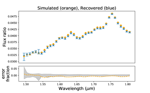
Figure 4: The resulting spectrum measured by MCMC fit over 39 parameters (flux ratio in 37 wavelength channels, separation, and position angle). The orange dots represent the simulated spectrum and the blue stars represent the spectrum recovered by this method with $1\sigma$ errors. The dashed orange line in the bottom panel shows the fractional error between the simulated and recovered spectrum, while the gray region shows the fractional error bounds.

4.2 Spectral Channel Correlations

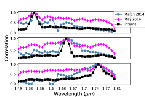
Figure 5: Phase correlations over spectral channel with respect to channels 6 (top), 18 (middle), and 30 (bottom), The internal source data (black squares) shows low levels of correlation except in the nearest neighboring channels. On sky images in March 2014 (blue circles), which saw better conditions, and in May 2014 (pink diamonds), which saw worse conditions, show larger correlation between channels.

Following Zimmerman et al. (2012) we can describe the correlation of closure phases between spectral channels. The average correlation is defined as:

$$C(q,w_{1};q,w_{2}) = \frac{\langle(\Psi_{q,w1}-\overline{\Psi}_{q,w1})(\Psi_{q,w2}-\overline{\Psi}_{q,w2})\rangle}{\sigma_{\Psi_{q,w1}}\sigma_{\Psi_{q,w2}}}$$ (6)

$$\overline{C}(w_{1};w_{2}) = \sum_{q=0}^{N_{CP-1}}\frac{Corr(q,w_{1};q,w_{2})}{N_{CP}}$$ (7)

Where $\Psi_{q,w_{i}}$ represents all the measured closure phases of the $q$th triplet at channel $w_{i}$, $\overline{\Psi}$ is the mean, and $\sigma$ is the standard deviation.

Zimmerman et al. (2012) showed large correlations between spectral channels across the band for P1640 (Oppenheimer et al., 2012) NRM IFS images. Some correlation is expected due to interpolation along the wavelength axis. The simulated dataset, generated from internal source data, does not suffer from atmospheric fluctuations. In this case we see a small amount of correlation between channels except for the nearest neighboring 2-3 channels (Figure 5). This is likely dominated by the interpolation. The internal source data provide an estimate the limiting performance of the instrument.

For on-sky data, depending on observing conditions we find higher levels of correlation between spectral channels, beyond the effect of interpolating the wavelength solution. In Figure 5 we also compare spectral channel correlations of the two on-sky datasets. In poor conditions (which also correspond to worse contrast sensitivity) we see a high amount of correlation across almost all spectral channels. This is likely the result of smearing of fringes due to vibration and/or non-static phase errors. We further discuss the differences between these data in Section 4.

4.3 GPI+NRM single source contrast performance

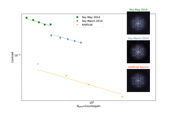
Figure 6: A summary of the median binary contrast sensitivity between $50-300$ mas for 3 datasets, on-sky observations of HD63852 during two different observing runs, and internal source exposures. The March observations showed significantly lower residual AO wavefront error, windspeed, and DIMM seeing. In better conditions we see both smaller phase errors and a sharper image, shown on the right inset plots. Table 3 shows a more complete list of environmental measurements. Plotted are the contrast sensitivity obtained with 6, 7, 8, 9 and 10 frames for the on-sky datasets, and 6, 10, 15, and 27 frames for the internal source dataset. The contrast values are plotted against total cumulative photon count in the corresponding frames based on a gain factor of 3.04. Dashed lines represent a $1/\sqrt{t}$ trend to compare with the measured contrasts.

In this section we discuss contrast sensitivity with respect to photon noise and varying conditions, and provide expected performance for future observations. In the best case, images taken with the internal source do not suffer atmospheric aberration and represent a baseline for performance. We expect these data to be primarily limited by photon and detector noise. On-sky observations will suffer from additional aberrations and smearing out of the image depending on weather conditions. Observations of an unresolved single star at two different times with different seeing and wind conditions provide an example of how performance can vary with conditions. We observed single star HD 63852 on two different nights in H band. As before, to obtain a proxy for calibrated contrast, we split each sequence of exposures in half and calibrate the first half against the second half. This likely overestimates the contrast sensitivity because it assumes no phase error differences between the target and calibrator. However, this exercise demonstrates trends in contrast performance with various environmental conditions and represents an ideal case. In a full science sequence one or more different unresolved sources will be used to calibrate the science target. Calibrators lie in different parts of the sky and the observations are separated in time between slew and acquisition. This leads to imperfect correction of closure phase errors.

In practice NRM contrast will be limited by a range of factors other than photon noise. Uncharacterized detector noise, vibrations, and imperfect AO correction that lead to smearing of fringes during an exposure integration can contribute to reduced contrast. To characterize the performance, for each set of observations, we measure closure phases and scatter with increasing photon count by analyzing partial datasets at a time, adding in consecutive exposures to increase total counts. In Fig. 6 we display the measured binary detection sensitivity against photons collected (detector counts divided by the recorded gain factor). We compare the measured contrast with a $1/\sqrt{t}$ trend and see some deviations that indicate other systematic errors in closure phase.

All dataset contrasts improve with increased exposure time but on-sky observations are not photon noise limited. The dominant error source in this case is likely time-varying aberrations and vibrations that reduce fringe visibility (smear out the PSF), resulting from a range of weather conditions that control the atmospheric turbulence times scale. Systematic errors are known to limit performance (phase errors) in aperture masking data (Lacour et al., 2011).

The first flux ratio minimum (H-band) is at $40\mathrm{mas}$. To compare, we report the average contrast measured between 100 and 300 mas for each dataset. For images taken with the internal source, contrast improves with increased exposure time following the photon noise limit $\sim\sqrt{N_{phot}}$. In a range of sky conditions, we see that other effects limit contrast. In very good conditions we find contrast sensitivity at SNR=5 close to $\Delta\mathrm{mag}$=7.5 at separations greater than $40\mathrm{mas}$. We found that in conditions with higher wind and low level turbulence we measure an order of magnitude reduced contrast sensitivity for the same bright source. These conditions generally correspond to Gemini Observatory IQANY conditions with high wind.

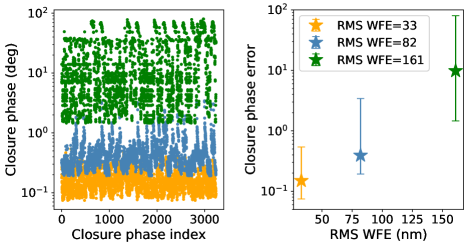
Figure 7: Phase errors compared to residual AO wavefront error (nm) for the three sets of observations compared in Figure 6. The left panel shows the error in each closure phase for every wavelength channel, while the right panel shows the RMS wavefront error measured from the wavefront sensor compared to the average closure phase error. Errorbars show the full range of closure phase errors measured for the dataset.

With few datapoints it is challenging to conclusively identify the dominant effect reducing fringe contrast, but there are a few obvious correlations. We note that residual AO wavefront error is a good predictor of point source contrast. In Figure 7 we show closure phase error as a function of the wavefront error value reported in the data headers. The cyclical nature of the phase errors follows a rough scaling with wavelength (also shown in Greenbaum et al., 2014). We also see a correlation with wind speed, however, the wind speed recorded in the header refers to surface-layer wind and does not provide any information on wind speed at other levels of the atmosphere. Madurowicz et al. (2018) show that the wind butterfly aberration seen by GPI’s coronagraph (Poyneer et al., 2016) most strongly correlates with wind at high altitudes. It is possible the higher altitude wind was also present during these observations, or that the ground-layer wind correlates with short characteristic timescales of atmospheric seeing, also shown to have a strong effect on GPI performance (Bailey et al., 2016).

On-sky observations of fainter targets not only reduces the number of photons collected, but contains more PSF jitter due to uncorrected wavefront and small changes in the PSF and/or uncorrected tip/tilt. This has the additional effect of blurring the image and reducing fringe contrast. This effect is strongest in poor conditions and especially high winds.

4.4 Resolving close binary HR2690

For basic validation of using the NRM to resolve point sources and obtain precise astrometry we observed the known binary HR 2690 during early commissioning of GPI. The primary HR 2690A is classified as a B3 star (Buscombe, 1969). The contrast ratio of the companion has been typically measured $\Delta\mathrm{mag}\sim 2$ at 0.543$\mu$m Mason et al. (1997). We observed the binary in the sequence Target-Calibrator-Calibrator. We measure a contrast sensitivity of $\sim 5\times 10^{-3}$ by calibrating our two single stars with each other.

We easily recover the binary in H band and measure a primary to secondary flux ratio of $5.7\pm 0.05$ ($\Delta\mathrm{mag}\sim 1.89$) a separation of $89.15\pm 0.12$ mas, and position angle of $192.29\pm 0.14^{\circ}$, after adding GPI plate scale and PA errors in quadrature. We find a slight spread in results depending on using one vs. both calibrators, within the errors.

HR 2690 B was first resolved by Mason et al. (1997) with speckle imaging. These observations were followed up several times over the next 19 years (Hartkopf et al., 2012; Tokovinin et al., 2014, 2015, 2016), all using speckle interferometry. We show the current astrometric positions relative to the primary including the GPI epoch in Figure 8. The GPI astrometry appears to be consistent with previous measurements. Small discrepancies in astrometry could point to a mismatch in absolute calibration.

Following the procedure outlined in §4.1, we fit astrometry and contrast in each wavelength channel. We find a fairly flat contrast spectrum over H band at $\Delta mag\sim 1.89$, which matches the reported $\Delta mag$ (Stromgren y filter at 0.543$\mu$m) from most of the previous studies (Mason et al., 1997; Tokovinin et al., 2014, 2015, 2016). Hartkopf et al. (2012) report $\Delta mag_{y}$=3.2, which is inconsistent with all other measurements. The similar flux ratio seen at both visible and near-IR wavelength indicate that the companion is also a hot star, probably late-B type given these contrast ratios.

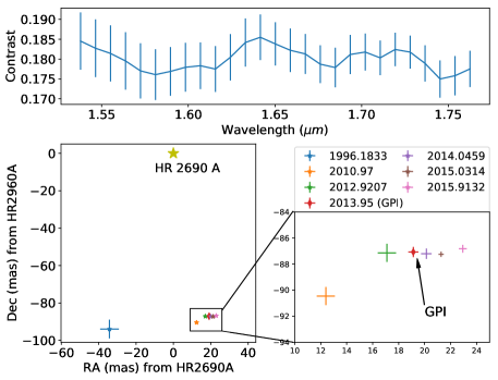
Figure 8: HR 2690 B Recovery. Top: Spectrum (contrast) of the HR 2690 companion measured as the ratio of the secondary to the primary. Bottom: Astrometry of HR 2690 including our GPI epoch. The yellow star marks the position of HR 2690 A.

As an independent check on our errorbars, we recover simulated signals using the two calibration sources. We inject and recover a signal into one of the calibration sources, HR 2839, and use the other, HR 2716, as a sole PSF calibrator. We simulate 10 datasets at different position angles near the separation recovered with the contrast ratio spectrum extracted from the HR 2690 binary. We follow the complete extraction procedure for each simulated dataset and compute the average and standard deviation. The errors computed by this approach, shown in Figure 9 (top), are consistent with $1\sigma$ errorbars computed in the original extraction. In this case there is also a slight bias in the recovered spectra to lower flux ratio, a factor $\sim 2-3\%$. For the position we compute a slightly higher error of $0.4~{}\mathrm{mas}$ and $0.4^{\circ}$ for separation and PA, respectively. The PA shows no strong bias, but the average recovered separation is approximately $0.4$ mas deviant from the input separation.

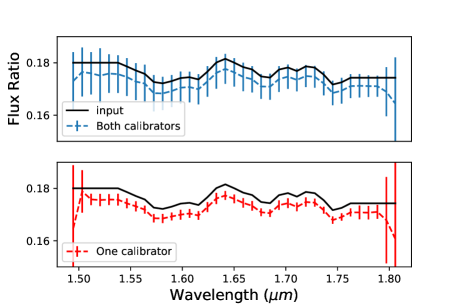
Figure 9: Injection recovery results when Top: simulated signals are injected into one calibration source and the data are calibrated using the second PSF calibrator. and Bottom: simulated signals are injected into one calibration source, and the same original source is used as the calibrator in the analysis. This simulates the case when only one useable calibration source is available for injection recovery analysis. In the first case the error in the recovered spectrum is consistent with $1-\sigma$ errors computed from the MCMC analysis for the spectrum, but there is a slight bias in the recovered contrast to smaller flux ratio. In the second case the errors are underestimated. the bias is consistent in both cases.

In some cases, only one PSF calibrator may be available so it is not possible to simulate a dataset that accounts for phase errors between sources. To highlight the difference, we repeat the injection recovery simulation by calibrating the simulated binary from HR 2839 data with the original HR 2839 data. As expected, the recovery errors are underestimated. The contrast ratio spectrum recovered in this simulation is shown in Figure 9. Interestingly, both the 2-calibrator simulation and this 1-calibrator simulation show the same “bias” in the recovered spectrum (shifted by $2-3\%$). In the case that only one calibration source is available, injection recovery can be used to measure a systematic offset in the parameters.

Using errors computed through injection recovery and mulitplying by the computed bias term we show the final spectrum and astrometry of our GPI epoch of observation in Figure 8. The flat spectrum over this short range is consistent with a late B-type companion. GPI NRM relative astrometry measurements are consistent with other high resolution observations and can reach precision of $\sim 0.5~{}\mathrm{mas}$ in separation and $\sim 0.5^{\circ}$ in PA.

4.5 Resolving M dwarf companion inside the transitional disk of HD 142527

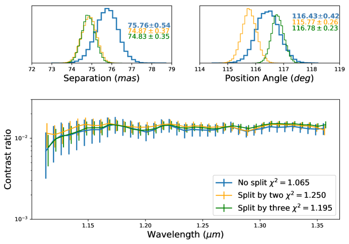
Figure 10: Simultaneous recovery of relative position and contrast ratio spectrum for three cases that use all 9 frames of data. The blue curves denote results obtained taking the average obervables over all 9 frames, considering the average baseline (average parallactic angle) over the observing sequence. The orange and green curves represent results when splitting the data by two and three parts, respectively, and combining/stacking those datasets, thus accounting for sky rotation over the observing sequence. The results were computed by adding $0.5\circ$ additional phase error in quadrature to the closure phase observables. Top: Posteriors for position parameters in each case. Errorbars reported are $1\sigma$ (not including GPI astrometry errors). All approaches, using the same updated calibration favor smaller separation and discrepant PA than the initial data reduction. The split cases, while producing tighter errorbars, are not consistent with each other, and lead to a poorer fit of the data. Bottom: The resulting contrast spectrum is consistent for each approach. Individual data points are slightly offset to display relative errorbars. Comparison of reduced $\chi^{2}$ shows that using the average of all the data provides the best fit in this case.

To demonstrate GPI NRM performance for detection and characterizion of faint companions at small angular separations, we observed the transitional disk-hosting, close binary system HD 142527. These data were first presented in Lacour et al. (2016). We present a new analysis here with more detail and compare the new spectrum in J-band to photometry and spectroscopy from other instruments. Since the second calibration source was determined to be a close binary (Le Bouquin, 2014) we only have one calibration source available for this analysis and the complete injection recovery approach to estimating errorbars is not possible. We perform the injection recovery to reveal any extraction biases, relying on $1\sigma$ errorbars computed by the MCMC reduction algorithm, which we have shown to be consistent with injection recovery errors in the previous example. Extraction biases are $\sim 5\%$, which we apply to the resulting spectrum for §4.5.2.

4.5.1 Recovering parameters

We first determine the position and average contrast ratio. We follow a similar procedure reported in Lacour et al. (2016), using all frames except two where the AO system lost lock on the star and the images are noticeably blurred. We use an average sky rotation and consider the whole dataset at this common parallactic angle. This position is in agreement with previously measured astrometry (Biller et al., 2012; Close et al., 2014; Lacour et al., 2016). We measure an average contrast ratio of $\sim 70$ between the primary and the secondary, which is consistent with measurements in J and H bands (Lacour et al., 2016) with NACO sparse aperture masking. Next we compute the full set of parameters, contrast ratio for each wavelength channel and position, as outlined in §4.1 adding $0.5^{\circ}$ additional closure phase error in quadrature. We obtain a projected separation of $75.76\pm 0.54~{}$mas and PA of $116.43\pm 0.44^{\circ}$ ($\chi^{2}=1.07$).

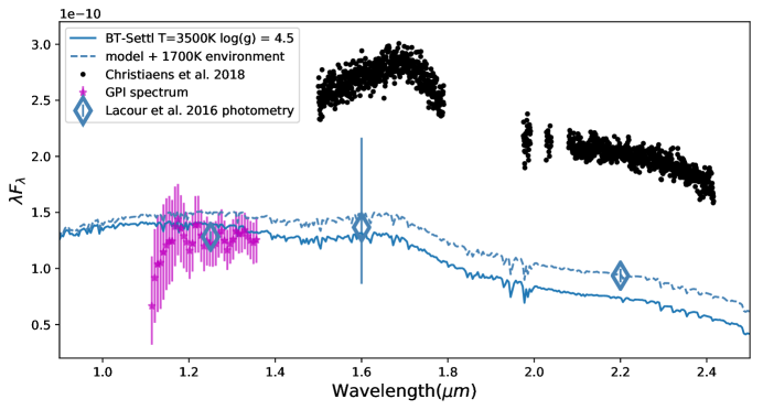
Figure 11: HD 142527 B spectrum converted to flux based on the host star photometry (blue diamonds) from Lacour et al. (2016). Blue lines represent model spectra described in Lacour et al. (2016) and Christiaens et al. (2018) with $T=3500\mathrm{K}$, $log(g)=4.5$, alone (solid) and with a 1700K environment (dashed), assuming a distance of 140pc. Our spectrum of HD 142527 B is consistent with this previously measured photometry, which are discrepant from new VLT/SINFONI H+K spectroscopy (Christiaens et al., 2018) displayed in black dots.

Since there is a significant amount of sky rotation (11.4^∘) over the course of the HD142527 integrations, we explored the effect of splitting the dataset into two groups of four and five exposures and three groups of three exposures, combining the rotated baselines in the analysis. We refer to this as the “split and combine” method. In this case the contrast ratio between HD142527 A and B is slightly higher. The parameter errorbars are also slightly smaller due to the larger number of observables. We recover slightly smaller separations of $74.83\pm 0.35~{}$mas and $74.87\pm 0.37~{}$mas and discrepant PAs of $115.8\pm 0.29^{\circ}$ and $116.8\pm 0.26^{\circ}$ for the split in two ($\chi^{2}=1.25$) and split in three ($\chi^{2}=1.19$) cases.

Next we use the three-parameter analysis results as a starting guess to simultaneously fit for position and a contrast ratio in each spectral channel for each of the three reduced datasets, the average of all frames, and the split and combined by two and three. The comparison is shown in Figure 10. The two split datasets still produce a smaller separation and discrepant PAs. However, all reduced datasets produce a consistent spectrum. A known degeneracy between separation and contrast could be the cause of a smaller recovered separation, but the discrepancy in PA is likely due poor data quality, since the results depend on how the data are combined. The small number of total frames makes this approach challenging.

While there is some variation in the position parameters, there is not a large difference in the spectrum of each reduction within the errorbars. We adopt the solution with the lowest error between the data and model (lowest $\chi^{2}$). Obtaining reliable astrometry may require more integrations in order to average out poor quality data and get a cleaner picture of the true astrophysical structure.

4.5.2 The HD 142527 B spectrum

H$\alpha$ was previously detected at visible wavelengths (Close et al., 2014), however, given our low resolution spectrum, our errors are too large to see the Pa$\beta$ signal expected accretion luminosity reported in either Close et al. (2014) (1.3% $L_{\odot}$) or Christiaens et al. (2018) (2.6% $L_{\odot}$). The expected line luminosity is approximately an order of magnitude smaller than our errorbars, according to the relations,

$$\log{(L_{acc})} = B+A\times L_{line}$$ (8)

$$A_{Pa\beta} = 1.36,B_{Pa\beta}=4.00$$ (9)

as described in Natta et al. (2004); Rigliaco et al. (2012).

We correct our recovered spectrum with the $\sim 5\%$ extraction bias factors computed from injection recovery in the calibration source dataset. The recovered spectrum is consistent with the broadband photometry previously measured for HD 142527 B (Biller et al., 2012; Lacour et al., 2016; Close et al., 2014). Figure 11 shows our J band spectrum next to published photometry (blue diamonds). We overplot a $T_{eff}=3500\mathrm{K}$ model alone and one with a 1700K environment (similar to the models described in Lacour et al. (2016) and Christiaens et al. (2018)), assuming a distance of 140 pc to be consistent with Lacour et al. (2016). Our results are consistent with the aperture masking detections. We also plot the higher resolution VLT/SINFONI H+K spectra from Christiaens et al. (2018) (black dots), and note the flux discrepancy. The discrepancy with Christiaens et al. (2018) is most likely a systematic error in one or both of the analyses. The presence of bright extended structures could bias the recovery of the secondary point source position and flux, but a point source was also detected in direct imaging (Close et al., 2014). Our results, taken independently, support previous aperture masking measurements, and we have demonstrated that our analysis procedure yields reliable measurement of the spectrum in simulations. Alternatively, it is possible that inaccurate calibration of the SINFONI data in post-processing could yield this discrepancy. The stellar spectrum models described in both studies assumed difference distances for HD 142527 B, $140\pm 20~{}$pc (Lacour et al., 2016) and $156\pm 6~{}$pc (Christiaens et al., 2018) resulting from the parallax measured with Gaia (Gaia Collaboration et al., 2016). We note the coincidence that the flux discrepancy is close to the scaling factor between these distances ($156^{2}/140^{2}$). If the deeper contrast measured from this and other aperture masking observations are correct, this may imply a lower effective temperature, or different circumbinary environment. The small separation of HD 142527 B makes non-coronagraphic, full pupil images challenging to reduce.

5 Polarimetric mode & visibility precision

Reliable visibility amplitudes are challenging to measure from the ground, even behind an extreme-AO system. Small temporal changes in phase smear fringes over individual integrations and vibrations artificially reduce amplitudes. Differential polarimetry enables self-calibrated amplitudes under the assumption that orthogonal polarization channels and rotated half-waveplate angles are expected to suffer the same systematic errors. These systematics can therefore be calibrated out to reveal different polarized structure. In this section we follow the polarimetry+NRM procedure outlined in Sec 3.3 and report performance of the NRM in polarimetric mode.

In commissioning the polarimetric mode we focused on single, unresolved calibration stars. The differential visibility signal is expected to be unpolarized and should show constant $\mathcal{V}_{diff}=1$ and $\phi_{CP}=0$ at all orientations. The deviation from the expected signal and scatter provide an estimate of both instrumental systematics and stability of the measurements. During commissioning observations in May 2015, when we experienced large vibrations, differential visibilities had very large errorbars and residual systematic scatter around $\mathcal{V}_{diff}=1$. Vibrations were exacerbated by high winds during May 2015 NRM commissioning.

In May 2016 commissioning, after a major source of vibration was fixed, we found that, in the best cases, differential visibilities calibrated to within $1\%$ of $\mathcal{V}=1$, $\sigma\sim 0.4\%$ in the best case shown here. Closure phases calibrated within $\sim 1-2^{\circ}$ for bright sources, $\sigma\sim 0.4^{\circ}$ in the best case. For example, Figure 12 shows the measured differential visibilities for single source HIP 74604 from data taken in GPI’s K1 band. This represents the best performance we achieved during commissioning, which is similar to the $\sigma\sim 0.4\%$ performance achieved with VAMPIRES polarimetry mode at visible wavelengths (Norris et al., 2015).

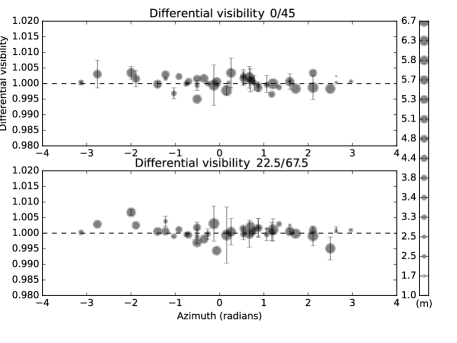
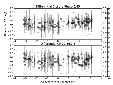
Figure 12: Differential visibilities (top) and differential closure phases (bottom) for a representative polarimetric dataset of a single, unpolarized star. Marker size scales with baseline length. We plot the differential visibility with baseline azimuthal orientation.

We explored the expected differential polarimetry signal of a protoplanetary disk by simulating the instrument response for a synthetic disk produced with MCFOST (Pinte et al., 2006, 2009) and reducing this simulated data through our pipeline. Within a limited set of tests attempting to simulate a relatively large signal, we were not able to simulate a detectable disk at the level of noise we measure from our best on-sky data, without artificially dialing down the flux from the star by a factor of a few. As an example (described in detail in Appendix B), we simulated data based modeling the features of HD 97048 (Lagage et al., 2006; Doucet et al., 2007), a young Herbig Ae star with a strong IR excess, $L_{IR}\sim 0.4L_{\odot}$ (Van Kerckhoven et al., 2002). We physically scale disk image so that the inner edge of the disk is located $<100~{}$mas from the central star. In this example, the integrated flux into one GPI pixel ($14.1~{}$mas) of the brightest part of the disk inner edge is still $\sim 7~{}$mag fainter than the host star (see Figure 13 in Appendix B).

6 Discussion

GPI’s non-redundant mask mode in general shows comparable performance compared to prior aperture masking (e.g. Lacour et al., 2011) and earlier IFS aperture masking (Zimmerman et al., 2012) experiments, and very good performance in good conditions that correspond to low residual WFE measured by the AO system. As Zimmerman et al. (2012) showed in the P1640 instrument, the IFS spectral axis provides improved overall contrast compared to broadband aperture masking and also smooths out baselines with lower sensitivity. This allows GPI NRM to reach contrasts close to $10^{-3}$ on bright targets and better than $10^{-2}$ on long individual integrations ($\sim$20-60 seconds). GPI’s NRM achieves similar performance at $\sim\lambda/D$ in J and H bands as NACO SAM L^′ imaging of similar total integration time, which achieved contrast limits of $2.5\times 10^{-3}$ (Lacour et al., 2011). Deeper NACO L^′ imaging (Gauchet et al., 2016) exceeds this sensitivity, especially for bright sources. GPI’s 10-hole mask, while reducing throughput compared to other masks with fewer holes provides fairly even coverage of spatial frequencies.

We find that, in addition to helping constrain the average contrast measurement, we can fit a spectrum reliably to moderate contrast sources, with improved overall contrast. We have presented new spectra of HR 2690 B in H band and HD 142527 B in J band that are consistent with previous photometry for both sources. A flux discrepancy remains between aperture masking observations of HD 142527 B and VLT/SINFONI spectra in H and K bands (Christiaens et al., 2018). Future observations may help resolve this discrepancy. GPI’s IFS mode combined with the NRM is particularly powerful for obtaining precise ($\sim\mathrm{few~{}mas}$) astrometry of companions around bright host stars that are separated $<100$ mas, where methods like Angular Differential Imaging (Marois et al., 2006) suffer.

The ability to resolve the relative astrometry and spectro-photometry of close binaries is a valuable tool for studying stellar multiplicity and calibrating evolutionary models as a function of mass and age. In addition, determining the mass and SED of both components of binary members of a moving group can constrain the age of the group as a whole, especially if a pre main sequence star is moving along the Henyey track (e.g. Nielsen et al. 2017). The best targets for this technique have short orbital periods to allow for quick characterization and large radial velocity signals, which in nearby moving groups means projected separations of $\sim$40 mas. Typical contrasts can reach masses $\sim 50M_{jup}$ for a very young bright target as we have shown in Figure 2 considering the AMES-Cond models (Baraffe et al. 2003) for a 1Myr 6.5 mag primary at 140pc.

In a single observing sequence, we obtained target integrations with minimal sky rotation, where possible, to provide multiple independent measurements along the same sky-projected baselines. In cases with a larger amount of sky rotation, we explored splitting up datasets to account for the rotation and take advantage of the increased Fourier coverage. While this can reduce the error on the fit, for the very small number of frames we obtained this produced discrepant results depending on how the data were split, sensitive to variations between frames. Ultimately averaging observables over all frames produced a better fit model for the HD 142527 dataset. All approaches yielded consistent spectra, but saw some variation in the relative position. With observations covering even greater sky rotation a split and combine approach will likely be neccesary and should be robust if the uncertainties on the observables can be estimated (e.g., by collecting a sufficient number of frames for each sky position).

Polarization mode observations rely on measuring stable amplitudes, which become degraded by vibrations and poor wavefront corrections. We saw improvement in precision after major sources of vibration were corrected. A faulty M2 mirror actuator was fixed and active dampers were installed. In the best case of the most recent observations, we measured precision of $\sigma\sim 0.4\%$ in differential visibilities and $\sim 0.4^{\circ}$ in differential closure phases in the best case. However, our limited observations make it difficult to characterize the typical polarimetric mode performance with the NRM on GPI. Initial attempts to simulate NRM images of a model protoplanetary disk did not yield a detectable signal; a disk will need to be relatively bright to be detected. Compared with the VAMPIRES instrument (Norris et al., 2015) we reach similar performance in our best dataset taken in K1 band. Typical VAMPIRES performance is likely better and their three-tier calibration (compared to GPI’s two-tier described in §3.3) makes that system more robust to systematic errors.

At this level of precision, young circumstellar disks may be a significant challenge to detect with differential polarimetry on GPI, compared to sources previously detected by this method with larger polarization signals (e.g., Norris et al., 2012a). In the case of a resolved signal with NRM+polarimetry, modeling is an essential component for recovering and interpreting the disk structure. Studying suspected polarized extended structures with NRM should be limited to the best conditions (low residual wavefront error, low wind). Future upgrades or instruments that can mitigate vibrations and tip/tilt errors for non-coronagraphic modes could make better use of polarimetry with NRM for studying circumstellar disks.

7 Summary and Conclusions

We have outlined the overall performance of the GPI NRM in IFS and polarimetric modes with a few example datasets. We have also described an open source software to reduce NRM fringes from GPI and other instruments and demonstrated results on various datasets. Future observations with the NRM on IFS instruments like GPI can use this study as a guideline for observing in these modes.

We also provide the following major takeaways for planning observations with GPI’s NRM:

• AO residual wavefront error correlates with NRM contrast performance (Fig. 6). The AOWFE header keyword is a good metric of conditions for NRM performance, given the “long” integration times.

• GPI NRM is suitable for moderate contrasts between $10^{2}-10^{3}$ to separations of $\sim 30\mathrm{mas}$, with degraded performance closer in.

• Ten holes provides good uv coverage minimizing gaps of sampling sensitivity, but at the cost of lower throughput.

• Polarization observations should be taken in conditions that minimize AO residual wavefront error and when vibrations can be minimized. Polarization observations should target objects with differential polarimetry signals $\gtrsim 1\%$.

This study can provide a comparison with other instruments using single-pupil interferometric methods (ie., NRM, kernel phase (Martinache, 2010)). Further improvements to the analyses presented in this work could be made by analyzing statistically independent kernel phases (i.e., Ireland, 2013) or with more sophisticated modeling and treatment of errors. The richness of the IFS datasets allows for varied approaches to treating and analyzing the data.

Ground-based NRM on instruments like GPI complement the capabilities of upcoming NIRISS aperture masking on JWST. The obvious advantage of NRM on ground-based facilities like GPI is in the larger telescope size that enables higher resolution sensitivity down to $10$s of milli-arcseconds. On the other hand, interferometric observations on a stable space telescope like JWST will carve out a different discovery space. The data will likely be photon-noise limited for bright sources, allowing at least an order of magnitude improved contrast compared to the ground. Space-based interferometric observations will also be able to complement ground-bases AO observations by observing sources too faint for visible wavefront sensors. Together with other high contrast and high resolution instruments, IFS aperture masking observations help to expand the detection landscape for direct imaging.

Appendix A Contrast spectra of HR 2690 B and HD 142527 B

We provide the contrast spectrum of HR 2690 B in Table 5 and HD 142527 B in Table 6. Absolute flux calibrations depend on the host star photometry and choice of model spectrum.

Table 5: Flux ratios recovered for HD 2690 B.

Wavelength ($\mu\mathrm{m}$)	Flux Ratio	$\mathrm{Error_{+}}$	$\mathrm{Error_{-}}$
1.537827643	0.180051769	0.006117792	0.005922433
1.546472049	0.178603929	0.005840979	0.006013181
1.555116455	0.177078709	0.005528977	0.005831117
1.563760975	0.175766975	0.005111043	0.005116699
1.572405381	0.172665394	0.005382201	0.005327732
1.581049787	0.172154242	0.005318425	0.005348661
1.589694307	0.173011673	0.005209509	0.005290487
1.598338713	0.174184211	0.005493067	0.005438636
1.606983119	0.174497753	0.005225567	0.005139819
1.615627639	0.173650569	0.004966511	0.004970789
1.624272045	0.176633443	0.004756046	0.004828567
1.632916451	0.180121456	0.004977992	0.004896766
1.641560971	0.181550508	0.00510479	0.005205588
1.650205377	0.180051944	0.005127553	0.00515305
1.658849783	0.178376985	0.004634255	0.004762568
1.667494303	0.177465747	0.004793606	0.004839009
1.676138709	0.174799634	0.004592341	0.004651037
1.684783115	0.174348035	0.004506974	0.004584267
1.693427635	0.177431085	0.004909268	0.004794985
1.702072041	0.178212043	0.00503311	0.004966011
1.710716447	0.176859468	0.005078732	0.004995903
1.719360966	0.178652942	0.004858403	0.004780304
1.728005373	0.178172915	0.004585516	0.004590963
1.736649779	0.175487526	0.004325864	0.004293816
1.745294298	0.171700648	0.00460216	0.004354205
1.753938704	0.172556787	0.004636444	0.004680254
1.762583111	0.174288292	0.004666991	0.004781194

Table 6: Flux ratios recovered for HD 142527 B.

Wavelength ($\mu\mathrm{m}$)	Flux Ratio	$\mathrm{Error_{+}}$	$\mathrm{Error_{-}}$
1.114073029	0.007267947	0.004835427	0.003762216
1.120800789	0.010011145	0.004738789	0.004379546
1.127528549	0.011327441	0.004793418	0.004649354
1.134256308	0.011465136	0.004688196	0.004493155
1.140984068	0.012490109	0.00464006	0.004623279
1.147711941	0.01316459	0.004552897	0.004364929
1.154439701	0.01355351	0.004379782	0.004214281
1.161167461	0.013537049	0.004000996	0.003915397
1.167895221	0.014960988	0.003871995	0.003850851
1.17462298	0.015653951	0.003427684	0.003493358
1.18135074	0.014759454	0.003214467	0.003288693
1.188078613	0.014018133	0.003213441	0.003124573
1.194806373	0.013425199	0.002869815	0.002900563
1.201534133	0.012590288	0.002839904	0.002744232
1.208261892	0.013288886	0.002762051	0.002728965
1.214989652	0.015046037	0.002809408	0.002681133
1.221717412	0.015079263	0.002792998	0.002698887
1.228445285	0.014030106	0.002514835	0.002558348
1.235173045	0.012988723	0.002492478	0.002426185
1.241900804	0.013489881	0.002361039	0.00236329
1.248628564	0.013230286	0.002148547	0.002178483
1.255356324	0.013107222	0.002199957	0.002087967
1.262084083	0.013264332	0.002177131	0.002152015
1.268811957	0.014177584	0.002082765	0.002253849
1.275539717	0.014503863	0.002086962	0.00215929
1.282267476	0.013568453	0.001929619	0.002003019
1.288995236	0.012662013	0.001967162	0.001922264
1.295722996	0.013277692	0.001895677	0.001937012
1.302450755	0.013703473	0.001951891	0.001962818
1.309178515	0.014498995	0.001914941	0.001903277
1.315906388	0.014245619	0.001920155	0.001907616
1.322634148	0.014284923	0.001862644	0.001861593
1.329361908	0.01462621	0.001683988	0.001860377
1.336089667	0.014070104	0.001864895	0.001855666
1.342817427	0.013637269	0.001885681	0.001836921
1.349545187	0.013433555	0.0019365	0.002086427
1.35627306	0.013692138	0.002108377	0.002229165

Appendix B Synthetic polarimetry observation example

To provide context for our reported precision we compared simulated data of a disk generated with MCFOST Pinte et al. (2006, 2009) based on modeling the features in HD 97048 Lagage et al. (2006); Doucet et al. (2007). For the purpose of this simulation we place the inner disk edge at $\sim 80~{}$mas extending out to $\sim 700~{}$mas. At a distance this corresponds to an inner edge at $\sim 9~{}$au, extending out to $\sim 116~{}$au. Figure 13 shows the model of the disk in total and polarized intensity as well as the “perfect” differential visibilities (Equation 5) over continuous spatial frequencies, by taking the Fourier transformation of the simulated disk Stokes parameters. The greatest azimuthal variation occurs between baselines of 1-2 m, where the disk is the most resolved. Given the symmetry of the disk, the differential closure phase signal is small ($<1^{\circ}$).

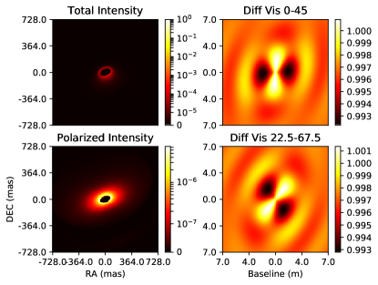
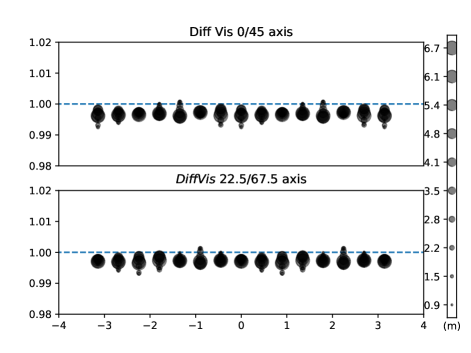
Figure 13: Left-most column: Disk model total and polarized intensity normalized to the same value. Middle column: Differential visibilities shown in spatial frequency space. Right: Continuously sampling the differential visibilities in azimuth. The NRM more sparsely samples this space.

To interpret differential visibility data it is helpful to forward model the resolved polarized structure and compare this to differential visbilities measured on sky. We outline the steps to generate a simulated set of GPI NRM data, converting from given Stokes I-V parameters, to linear polarization images at four half-wave plate angles $0^{o}$, $22.5^{o}$, $45^{o}$, and $67.5^{o}$. The intensity images are computed as follows:

$$I_{\pm}(0^{o})=\frac{I\pm Q}{2};I_{\pm}(22.5^{o})=\frac{I\pm U}{2}$$

$$I_{\pm}(45^{o})=\frac{I\mp Q}{2};I_{\pm}(67.5^{o})=\frac{I\mp U}{2}$$

where (+,-) denotes the two polarization channels split by the Wollaston prism. Each intensity is convolved with the GPI PSF accounting for some photon noise and a small amount of jitter by convolving the image with a Gaussian of the size of the desired jitter. In practice, however, vibrations are not uniform in time or direction. They are mitigated by observing in low-wind conditions.

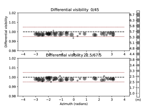
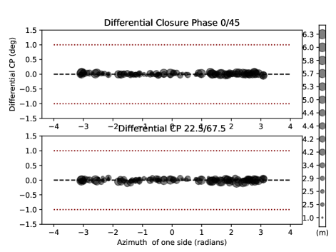
Figure 14: Differential observables measured from simulated low-noise GPI data containing the disk model. Marker sizes denote the baseline length, where the largest circles represent the longest baseline formed by the mask. The left shows the measured differential visibilities. The red dotted lines mark 0.5% scatter, such as differential visibilities measured in the best case for an unresolved star. The right shows differential closure phases measured from the same simulated data. The red dotted lines mark $1^{\circ}$ of scatter, similar to the scatter shown in Figure 12. For polarized structure that is highly symmetric, differential visibilities are a more sensitive observable.

We measure fringe observables from the simulated data and compare these to the “perfect” visibilities in Figure 14. In this low-noise simulation we can clearly see the disk and inner cavity are resolved by the raw visibilities. This will not necessarily be the sky with real data, especially when large vibrations are present. The mask baselines show similar variation with baseline orientation as the “perfect” visibilites. In practice, reconstructing disk features will likely rely on forward modeling of the disk as we show here (First described in Norris et al., 2012b, 2015).

References

- Allard et al. (2003) Allard, F., Guillot, T., Ludwig, H.-G., et al. 2003, in Brown Dwarfs, Vol. 211, 325
- Astropy Collaboration et al. (2013) Astropy Collaboration, Robitaille, T. P., Tollerud, E. J., et al. 2013, A&A, 558, A33, doi: 10.1051/0004-6361/201322068
- Bailey et al. (2016) Bailey, V. P., Poyneer, L. A., Macintosh, B. A., et al. 2016, in Adaptive Optics Systems V, Vol. 9909, 99090V
- Baldwin et al. (1986) Baldwin, J. E., Haniff, C. A., Mackay, C. D., & Warner, P. J. 1986, Nature, 320, 595, doi: 10.1038/320595a0
- Baraffe et al. (2003) Baraffe, I., Chabrier, G., Barman, T. S., Allard, F., & Hauschildt, P. H. 2003, A&A, 402, 701, doi: 10.1051/0004-6361:20030252
- Beuzit et al. (2008) Beuzit, J.-L., Feldt, M., Dohlen, K., et al. 2008, in Proc. SPIE, Vol. 7014, Ground-based and Airborne Instrumentation for Astronomy II, 701418
- Biller et al. (2012) Biller, B., Lacour, S., Juhász, A., et al. 2012, ApJ, 753, L38, doi: 10.1088/2041-8205/753/2/L38
- Buscombe (1969) Buscombe, W. 1969, MNRAS, 144, 31, doi: 10.1093/mnras/144.1.31
- Cheetham et al. (2015) Cheetham, A., Huélamo, N., Lacour, S., de Gregorio-Monsalvo, I., & Tuthill, P. 2015, MNRAS, 450, L1, doi: 10.1093/mnrasl/slv033
- Christiaens et al. (2018) Christiaens, V., Casassus, S., Absil, O., et al. 2018, ArXiv e-prints, arXiv:1806.04792. https://arxiv.org/abs/1806.04792
- Close et al. (2014) Close, L. M., Follette, K. B., Males, J. R., et al. 2014, ApJ, 781, L30, doi: 10.1088/2041-8205/781/2/L30
- De Rosa et al. (2015) De Rosa, R. J., Nielsen, E. L., Blunt, S. C., et al. 2015, ApJ, 814, L3, doi: 10.1088/2041-8205/814/1/L3
- Doucet et al. (2007) Doucet, C., Habart, E., Pantin, E., et al. 2007, A&A, 470, 625, doi: 10.1051/0004-6361:20066610
- Doyon et al. (2012) Doyon, R., Hutchings, J. B., Beaulieu, M., et al. 2012, in Proc. SPIE, Vol. 8442, Space Telescopes and Instrumentation 2012: Optical, Infrared, and Millimeter Wave, 84422R
- Duchêne et al. (2018) Duchêne, G., Lacour, S., Moraux, E., Goodwin, S., & Bouvier, J. 2018, MNRAS, 478, 1825, doi: 10.1093/mnras/sty1180
- Foreman-Mackey et al. (2013a) Foreman-Mackey, D., Hogg, D. W., Lang, D., & Goodman, J. 2013a, Publications of the Astronomical Society of the Pacific, 125, 306, doi: 10.1086/670067
- Foreman-Mackey et al. (2013b) Foreman-Mackey, D., Conley, A., Meierjurgen Farr, W., et al. 2013b, emcee: The MCMC Hammer, Astrophysics Source Code Library. http://ascl.net/1303.002
- Gaia Collaboration et al. (2016) Gaia Collaboration, Brown, A. G. A., Vallenari, A., et al. 2016, A&A, 595, A2, doi: 10.1051/0004-6361/201629512
- Gauchet et al. (2016) Gauchet, L., Lacour, S., Lagrange, A.-M., et al. 2016, A&A, 595, A31, doi: 10.1051/0004-6361/201526404
- Greenbaum (2018) Greenbaum, A. 2018, ImplaneIA: Tools for fitting (image plane fringes), calibrating, and analyzing NRM data across multiple instruments and modes, 1.0.0, Zenodo, doi: 10.5281/zenodo.2530787. https://doi.org/10.5281/zenodo.2530787
- Greenbaum et al. (2015) Greenbaum, A. Z., Pueyo, L., Sivaramakrishnan, A., & Lacour, S. 2015, ApJ, 798, 68, doi: 10.1088/0004-637X/798/2/68
- Greenbaum et al. (2018) Greenbaum, A. Z., Sivarmakrishnan, A., Sahlmann, J. S., & Thatte, D. 2018, ImPlaneIA: Image Plane Approach to Interferometric Analysis, Astrophysics Source Code Library. http://ascl.net/1808.004
- Greenbaum et al. (2014) Greenbaum, A. Z., Cheetham, A., Sivaramakrishnan, A., et al. 2014, in Proc. SPIE, Vol. 9147, Ground-based and Airborne Instrumentation for Astronomy V, 91477B
- Hartkopf et al. (2012) Hartkopf, W. I., Tokovinin, A., & Mason, B. D. 2012, AJ, 143, 42, doi: 10.1088/0004-6256/143/2/42
- Ireland (2013) Ireland, M. J. 2013, MNRAS, 433, 1718, doi: 10.1093/mnras/stt859
- Jennison (1958) Jennison, R. C. 1958, MNRAS, 118, 276, doi: 10.1093/mnras/118.3.276
- Jones et al. (2001) Jones, E., Oliphant, T., Peterson, P., et al. 2001, SciPy: Open source scientific tools for Python. http://www.scipy.org/
- Konopacky et al. (2014) Konopacky, Q. M., Thomas, S. J., Macintosh, B. A., et al. 2014, in Society of Photo-Optical Instrumentation Engineers (SPIE) Conference Series, Vol. 9147, Ground-based and Airborne Instrumentation for Astronomy V, 914784
- Kraus & Ireland (2012) Kraus, A. L., & Ireland, M. J. 2012, ApJ, 745, 5, doi: 10.1088/0004-637X/745/1/5
- Kraus et al. (2008) Kraus, A. L., Ireland, M. J., Martinache, F., & Lloyd, J. P. 2008, ApJ, 679, 762, doi: 10.1086/587435
- Lacour et al. (2011) Lacour, S., Tuthill, P., Amico, P., et al. 2011, A&A, 532, A72, doi: 10.1051/0004-6361/201116712
- Lacour et al. (2016) Lacour, S., Biller, B., Cheetham, A., et al. 2016, A&A, 590, A90, doi: 10.1051/0004-6361/201527863
- Lagage et al. (2006) Lagage, P.-O., Doucet, C., Pantin, E., et al. 2006, Science, 314, 621, doi: 10.1126/science.1131436
- Le Bouquin (2014) Le Bouquin, J. B. 2014, ArXiv e-prints, arXiv:1408.3227. https://arxiv.org/abs/1408.3227
- Liu et al. (2010) Liu, M. C., Wahhaj, Z., Biller, B. A., et al. 2010, in Adaptive Optics Systems II, Vol. 7736, 77361K
- Macintosh et al. (2014) Macintosh, B., Graham, J. R., Ingraham, P., et al. 2014, Proceedings of the National Academy of Science, 111, 12661, doi: 10.1073/pnas.1304215111
- Madurowicz et al. (2018) Madurowicz, A., Macintosh, B. A., Ruffio, J.-B., et al. 2018, ArXiv e-prints, arXiv:1807.07179. https://arxiv.org/abs/1807.07179
- Marois et al. (2006) Marois, C., Lafrenière, D., Doyon, R., Macintosh, B., & Nadeau, D. 2006, ApJ, 641, 556, doi: 10.1086/500401
- Martinache (2010) Martinache, F. 2010, ApJ, 724, 464, doi: 10.1088/0004-637X/724/1/464
- Mason et al. (1997) Mason, B. D., ten Brummelaar, T., Gies, D. R., Hartkopf, W. I., & Thaller, M. L. 1997, AJ, 114, 2112, doi: 10.1086/118630
- Monnier (1999) Monnier, J. D. 1999, PhD thesis, University of California, Berkeley
- Natta et al. (2004) Natta, A., Testi, L., Muzerolle, J., et al. 2004, A&A, 424, 603, doi: 10.1051/0004-6361:20040356
- Norris et al. (2015) Norris, B., Schworer, G., Tuthill, P., et al. 2015, MNRAS, 447, 2894, doi: 10.1093/mnras/stu2529
- Norris et al. (2012a) Norris, B. R. M., Tuthill, P. G., Ireland, M. J., et al. 2012a, Nature, 484, 220, doi: 10.1038/nature10935
- Norris et al. (2012b) Norris, B. R. M., Tuthill, P. G., Ireland, M. J., et al. 2012b, in Optical and Infrared Interferometry III, Vol. 8445, 844503
- Oppenheimer et al. (2012) Oppenheimer, B. R., Beichman, C., Brenner, D., et al. 2012, in Proc. SPIE, Vol. 8447, Adaptive Optics Systems III, 844720
- Perrin et al. (2014) Perrin, M. D., Maire, J., Ingraham, P., et al. 2014, in Proc. SPIE, Vol. 9147, Ground-based and Airborne Instrumentation for Astronomy V, 91473J
- Perrin et al. (2015) Perrin, M. D., Duchene, G., Millar-Blanchaer, M., et al. 2015, ApJ, 799, 182, doi: 10.1088/0004-637X/799/2/182
- Pinte et al. (2009) Pinte, C., Harries, T. J., Min, M., et al. 2009, A&A, 498, 967, doi: 10.1051/0004-6361/200811555
- Pinte et al. (2006) Pinte, C., Ménard, F., Duchêne, G., & Bastien, P. 2006, A&A, 459, 797, doi: 10.1051/0004-6361:20053275
- Poyneer et al. (2016) Poyneer, L. A., Palmer, D. W., Macintosh, B., et al. 2016, Appl. Opt., 55, 323, doi: 10.1364/AO.55.000323
- Rigliaco et al. (2012) Rigliaco, E., Natta, A., Testi, L., et al. 2012, A&A, 548, A56, doi: 10.1051/0004-6361/201219832
- Rizzuto et al. (2016) Rizzuto, A. C., Ireland, M. J., Dupuy, T. J., & Kraus, A. L. 2016, Astrophysical Journal, 817, 164, doi: 10.3847/0004-637X/817/2/164
- Sallum et al. (2015a) Sallum, S., Follette, K. B., Eisner, J. A., et al. 2015a, Nature, 527, 342, doi: 10.1038/nature15761
- Sallum et al. (2015b) Sallum, S., Eisner, J. A., Close, L. M., et al. 2015b, ApJ, 801, 85, doi: 10.1088/0004-637X/801/2/85
- Sana et al. (2014) Sana, H., Le Bouquin, J. B., Lacour, S., et al. 2014, The Astrophysical Journal Supplement Series, 215, 15, doi: 10.1088/0067-0049/215/1/15
- STScI Development Team (2013) STScI Development Team. 2013, pysynphot: Synthetic photometry software package. http://ascl.net/1303.023
- Tokovinin et al. (2014) Tokovinin, A., Mason, B. D., & Hartkopf, W. I. 2014, AJ, 147, 123, doi: 10.1088/0004-6256/147/5/123
- Tokovinin et al. (2015) Tokovinin, A., Mason, B. D., Hartkopf, W. I., Mendez, R. A., & Horch, E. P. 2015, AJ, 150, 50, doi: 10.1088/0004-6256/150/2/50
- Tokovinin et al. (2016) —. 2016, AJ, 151, 153, doi: 10.3847/0004-6256/151/6/153
- Tuthill et al. (1999) Tuthill, P. G., Monnier, J. D., & Danchi, W. C. 1999, Nature, 398, 487, doi: 10.1038/19033
- Tuthill et al. (2000) Tuthill, P. G., Monnier, J. D., Danchi, W. C., Wishnow, E. H., & Haniff, C. A. 2000, PASP, 112, 555, doi: 10.1086/316550
- van der Walt et al. (2011) van der Walt, S., Colbert, S. C., & Varoquaux, G. 2011, Computing in Science and Engineering, 13, 22, doi: 10.1109/MCSE.2011.37
- Van Kerckhoven et al. (2002) Van Kerckhoven, C., Tielens, A. G. G. M., & Waelkens, C. 2002, A&A, 384, 568, doi: 10.1051/0004-6361:20011814
- Wolff et al. (2014) Wolff, S. G., Perrin, M. D., Maire, J., et al. 2014, in Ground-based and Airborne Instrumentation for Astronomy V, Vol. 9147, 91477H
- Zimmerman et al. (2012) Zimmerman, N., Sivaramakrishnan, A., Bernat, D., et al. 2012, in Proc. SPIE, Vol. 8445, Optical and Infrared Interferometry III, 84452G