Equivariant mappings and invariant sets
on Minkowski space

Abstract

In this paper we introduce the systematic study of invariant functions and equivariant mappings defined on Minkowski space under the action of the Lorentz group. We adapt some known results from the orthogonal group acting on the Euclidean space to the Lorentz group acting on the Minkowski space. In addition, an algorithm is given to compute generators of the ring of functions that are invariant under an important class of Lorentz subgroups, namely when these are generated by involutions, which is also useful to compute equivariants. Furthermore, general results on invariant subspaces of the Minkowski space are presented, with a characterization of invariant lines and planes in the two lowest dimensions.

Miriam Manoel

Departamento de Matemática, ICMC

Universidade de São Paulo

13560-970 Caixa Postal 668, São Carlos, SP - Brazil

Leandro N. Oliveira

Centro de Ciências Exatas e Tecnológicas - CCET, UFAC

Universidade Federal do Acre

69920-900 Rod. BR 364, Km 04, Rio Branco - AC, Brazil

Keywords. symmetry, Lorentz group, Minkowski space, group representation.

2010 MSC. 22E43, 51B20, 13A50.

1 Introdution

The interest of studying the effect of symmetries in a mathematical model is common sense. They frequently appear in the applications, in general as a result of the geometry of the configuration domain, the modeling assumptions, the method to reducing to normal forms and so on. In dynamical systems, certain observations are tipically related to patterns of symmetry, namely degeneracy of solutions, high codimension bifurcations, unexpected stabilities, phase relations, synchrony in coupled systems and periodicity of solutions. These phenomena, not expected in absence of symmetries, can be predicted once the inherent symmetries are taken into account in the model formulation. This observation has stimulated the great achievements in the theory of equivariant dynamical systems during the last decades. The set-up is based on group representation theory, once the set formed by these symmetries has a group structure. We mention for example the works in [1, 2, 3, 4] where algebraic invariant theory is used to derive the general form of equivariant mappings that define vector fields on real or complex Euclidean $n$-dimensional vector spaces under the action of subgroups of the orthogonal group ${\bf O}(n)$, $n\geq 2$. A numerical analysis of such systems through computational programming has also been done, after the pionner works in [10, 11, 20]. Steady-state bifurcation, Hopf bifurcation, classification of equivariant singularities among other subjects have also been extensively studied in isolated dynamical systems or in networks of dynamical systems, for which we cite [2, 3, 7, 8, 15, 16, 19, GS06, 12] and hundreds of references therein.

The results in the present work go in a related but distinct direction. We use tools from group representation and from invariant theory to introduce a systematic study of symmetries of problems defined on the Minkowski space $\mathbb{R}^{n+1}_{1}$, $n\geq 1$. This is the $(n+1)$-dimensional real vector space $\mathbb{R}^{n+1}$ endowed with the pseudo inner product $\left<,\right>:\mathbb{R}^{n+1}_{1}\times\mathbb{R}^{n+1}_{1}\longrightarrow\mathbb{R}$ of signature $(n,1)$,

$$\left<x,y\right>=x^{t}Jy=\sum_{i=1}^{n}x_{i}y_{i}-x_{n+1}y_{n+1},$$

where

$$J=\left(\begin{array}[]{cc}I_{n}&0\\ 0&-1\end{array}\right),$$

also denoted by $I_{n,1}$, and $I_{n}$ denoting the identity matrix of order $n$. This generalizes the spacetime $\mathbb{R}^{4}_{1}$, which is the mathematical structure on which Einstein’s theory of relativity is formulated. In Minkowski space, the spatio-temporal coordinates of different observers are related by Lorentz transformations, so any laws for systems in Minkowski spacetime must accordingly be Lorentz invariant [14]. The group of symmetries is assumed to be a subgroup of the Lorentz group

$${\bf O}(n,1)=\left\{A\in GL\left(n+1,\mathbb{R}\right):A^{t}JA=J\right\},$$

formed by isometries of $\mathbb{R}^{n+1}_{1}$; here the superscript $t$ denotes transposition. We consider the standard action of (subgroups of) ${\bf O}(n,1)$ on $\mathbb{R}^{n+1}_{1}$, namely given by matrix multiplication. We use algebraic invariant theory and group representation to deduce the basic general results for the systematic study of mappings with symmetries defined on Minkowski space. We refer to [5] and [6] for example for potential applications of our results in the context with symmetries.

Many previous results for the Euclidean case adapt for our context in a natural way. The first to mention is a way to obtain equivariant mappings on $\mathbb{R}^{n+1}_{1}$ under the action of a subgroup $\Gamma<{\bf O}(n,1)$ from invariant functions under the diagonal action of same group defined on a cartesian product $\mathbb{R}^{n+1}_{1}\times\mathbb{R}^{n+1}_{1}$ (Theorem 2.2). We also adapt and extend [3, Theorem 3.2], regarding the construction of the general forms of functions invariant under a class of Lorentz subgroups, given by Algorithms 2.4, using Reynolds operators.

There are however two new structures here, namely the pseudo inner product and the distinct group structure of the set of symmetries, leading to new facts. For example, for an arbitrary Lorentz subgroup $\Gamma$, not all Minkowski subspace $W\subset\mathbb{R}^{n+1}_{1}$ admits its orthogonal subspace $W^{\perp}$ (with respect to the pseudo inner product) as an invariant complement under the action of $\Gamma$; for the Euclidean case see [12, Propostion XII, 2.1]. In fact, we proof that this holds, namely that $W\oplus W^{\perp}=\mathbb{R}^{n+1}_{1}$ with both $\Gamma$-invariant, if, and only if, $W$ is $\Gamma$-invariant and nondegenerate with respect to the pseudo inner product (Proposition 3.2). In addition, we give a sufficient condition for a degenerate subspace to admit an invariant complement (Proposition 3.3). In Section 3 we characterize the invariant subspaces for the lowest dimensions $n=1,2$ using, in the second case, the singular value decomposition of elements of the Lorentz group. This classification is directly related to the structure of the Lorentz group: let ${\bf SO}_{0}(n,1)$ denote the connected component of the identity and consider the elements (which we denote following the usual notation in the literature, as in ([9] for example),

$$\Lambda^{p}=\left(\begin{array}[]{cc}I_{n-1,1}&0\\ 0&1\end{array}\right),\ \ \ \Lambda^{t}=J.$$

We use the decomposition of ${\bf O}(n,1)$ as a semi-direct product,

$${\bf O}(n,1)={\bf SO}_{0}(n,1)\rtimes\left({\bf Z}_{2}(\Lambda^{t})\times{\bf Z}_{2}(\Lambda^{p})\right),$$ (1)

or, in other words, as the disjoint union

$${\bf O}(n,1)={\bf SO}_{0}(n,1)\dot{\cup}\Lambda^{p}{\bf SO}_{0}(n,1)\dot{\cup}\Lambda^{t}{\bf SO}_{0}(n,1)\dot{\cup}\Lambda^{pt}{\bf SO}_{0}(n,1),$$ (2)

where $\Lambda^{pt}=\Lambda^{p}\Lambda^{t}$. We then use this decomposition to identify conjugacy classes of Lorentz subgroups, once subgroups in distinct connected components are nonconjugate. We also give the type of each possible invariant subspaces, namely, as spacelike, timelike or lightlike subspaces, and recognize which are fixed-point subspaces of Lorentz subgroups.

Here is what comes in the following sections. Section 2 is devoted to invariant functions and equivariant mappings under subgroups of ${\bf O}(n,1)$. The two main results are Theorem 2.2, used to compute equivariants, and the algorithm presented in Subsection 2.1, used to compute invariants under a class of groups generated by involutions. An example in Subsection 2.2 illustrates both methods. In Section 3 we present general results about invariant subspaces and their orthogonal complements, with special attention to fixed-point subspaces. The subjects of Subsections 3.1 and 3.2 are the invariant subspaces in the Minkowski plane and Minkowski 3-dimensional space.

2 Invariant functions, equivariant mappings

The aim of this section is to give results on the construction of invariant functions and equivariant mappings under the action of a Lorentz subgroup $\Gamma$. We adapt some results from invariant theory on Euclidean space for the Minkowski space. We point out that the results are algebraic in nature, so they hold for functions and mappings defined on any subspace of $W\subseteq\mathbb{R}^{n+1}_{1}$ as long as it is $\Gamma$-invariant, namely, $\gamma x\in W$ for all $\gamma\in\Gamma$, $x\in W$. For simplification, from now on we assume the domain to be the whole $\mathbb{R}^{n+1}_{1}$.

A function $f:\mathbb{R}^{n+1}_{1}\rightarrow\mathbb{R}$ is called $\Gamma$-invariant if

$$f(\gamma x)=f(x),\quad\forall\gamma\in\Gamma,\quad\forall x\in\mathbb{R}^{n+1}_{1}.$$

The set of $\Gamma$-invariant functions is a ring, which we shall denote $\mathcal{I}(\Gamma)$. A map $g:\mathbb{R}^{n+1}_{1}\to\mathbb{R}^{n+1}_{1}$ is $\Gamma$-equivariant if it commutes with the action of $\Gamma$, that is, if

$$g(\gamma x)=\gamma g(x)\quad\forall\gamma\in\Gamma,\quad\forall x\in\mathbb{R}^{n+1}_{1}.$$

The set of $\Gamma$-equivariant maps is a module over the ring $\mathcal{I}(\Gamma)$, denoted here by ${\mathcal{M}}(\Gamma)$.

In the Euclidean context it is well-known that if $f:\mathbb{R}^{n}\to\mathbb{R}$ is invariant under the action of a subgroup of the orthogonal group ${\bf O}(n)$, then the gradient $\nabla f:\mathbb{R}^{n}\to\mathbb{R}^{n}$ is an equivariant map under this action. The corresponding result for the Lorentz group ${\bf O}(n,1)$ is given in Proposition 2.1, which can be used as a starting point to find generators for the module of equivariants if generators of the ring of invariants are known:

Proposition 2.1.

Let $\Gamma$ be a subgroup of ${\bf O}(n,1)$ and $f:\mathbb{R}^{n+1}_{1}\to\mathbb{R}$ $\Gamma$-invariant. Then $J\nabla f$ is a $\Gamma$-equivariant map.

Proof.

The equality $f(\gamma x)=f(x)$ implies $\gamma^{t}\nabla(f(\gamma x))=\nabla(f(x))$. Now just multiply both sides by $\gamma J$. ∎

The following result shows that a $\Gamma$-equivariant mapping $\mathbb{R}^{n+1}_{1}\to\mathbb{R}^{n+1}_{1}$ can be given from a $\Gamma$-invariant function $\mathbb{R}^{n+1}_{1}\times\mathbb{R}^{n+1}_{1}\to\mathbb{R}$ on the cartesian product, and vice-versa. The proof is constructive and follows the idea of the proof of [12, Theorem 6.8], providing a formula to construct one from the other.

Theorem 2.2.

Let $\Gamma$ be a subgroup of the Lorentz group ${\bf O}(n,1)$. There is a one-to-one correspondence between $\Gamma$-equivariant mappings $\mathbb{R}^{n+1}_{1}\to\mathbb{R}^{n+1}_{1}$ and $\Gamma$-invariant functions $\mathbb{R}^{n+1}_{1}\times\mathbb{R}^{n+1}_{1}\to\mathbb{R}$ under the diagonal action.

Proof.

Given $g:\mathbb{R}^{n+1}_{1}\to\mathbb{R}^{n+1}_{1}$, take $f:\mathbb{R}^{n+1}_{1}\times\mathbb{R}^{n+1}_{1}\to\mathbb{R},$

$$f(x,y)=\left<g(x),y)\right>.$$ (3)

This implies that

$$g(x)=J\left(d_{y}f\right)^{t}_{(x,0)}.$$ (4)

If $g$ is $\Gamma$-equivariant, then for the diagonal action of $\Gamma$ on $\mathbb{R}^{n+1}_{1}\times\mathbb{R}^{n+1}_{1}$ we have, for all $\gamma\in\Gamma$,

$$f(\gamma(x,y))=\left<g(\gamma x),\gamma y\right>=\left<\gamma g(x),\gamma y\right>=f(x,y).$$

Conversely, for any $\gamma\in\Gamma$, if $f$ is $\Gamma$-invariant, then, differenting $f(\gamma x,\gamma y)=f(x,y)$ at both sides with respect to $y$ at $(x,0)$,

$$\left(d_{y}f\right)_{(\gamma x,0)}\gamma=\left(d_{y}f\right)_{(x,0)}.$$

Taking the transpose,

$$g(\gamma x)=J\left(\gamma^{t}\right)^{-1}Jg(x),$$

so the result holds, since $J\left(\gamma^{t}\right)^{-1}J=\gamma$. ∎

The next result is our method to find a set of generators for the module of equivariant mappings:

Corollary 2.3.

If $\{u_{i},i=1,\ldots s\}$ is a set of generators of the ring of $\Gamma$-invariant functions $\mathbb{R}^{n+1}_{1}\times\mathbb{R}^{n+1}_{1}\to\mathbb{R}$ under the diagonal action, then

$$J\left(d_{y}u_{i}\right)_{(x,0)}^{t},\ i=1,\ldots,s$$

form a set of generators of the module ${\mathcal{M}}(\Gamma)$ over ${\mathcal{I}}(\Gamma)$ .

Proof.

For $g\in{\mathcal{M}}(\Gamma)$, we take $f$ as in (3). By hypothesis,

$$f(x,y)=h(u_{1}(x,y),\cdots,u_{s}(x,y)),$$

for some $h:\mathbb{R}^{s}\to\mathbb{R}$. This implies, using (4), that

$$g(x)=\sum_{i=0}^{s}\frac{\partial h}{\partial X_{i}}(u_{1},\cdots,u_{s})|_{y=0}\cdot J\left(d_{y}u_{i}\right)^{t}_{(x,0)},$$

where $X=(X_{1},\ldots,X_{s})\in\mathbb{R}^{s}$. So the result follows, since ${\partial h}/{\partial X_{i}}(u_{1}(x,0),\cdots,u_{s}(x,0))\in{\mathcal{I}}(\Gamma)$, $i=1,\ldots s$. ∎

This result is illustrated with an example, presented in Subsection 2.2.

2.1 An algorithm to compute invariants under subgroups containing involutions

For the following, recall that an involution is an invertible map which is its own inverse. Involutions in ${\bf O}(n,1)$ are order-2 matrices, also called generalized reflections. The aim here is to present Algorithm 2.4 which gives generators of the ring of invariant functions under the class of Lorentz subgroups $\Gamma<{\bf O}(n,1)$ that are generated by a finite set of involutions. More generally, we consider

$$\Gamma=\Sigma\rtimes\Delta,$$ (5)

for $\Sigma<\Gamma$ a subgroup such that ${\cal I}(\Sigma)$ is finitely generated and for $\Delta=[\delta_{1},\ldots,\delta_{m}]<\Gamma$ generated by involutions, $\delta_{i}^{2}=I$, $i=1,\ldots,m$, $m\geq 1$. More precisely, we deduce generators under the whole group from the generators under the subgroup $\Sigma$. This result generalizes [2, Theorem 4.5], obtained for $m=1$, in which case $\Gamma=\Sigma_{1}\rtimes{\bf Z}_{2}(\delta)$. Recall the two Reynolds operators on the ring of invariants $R,S:{\cal I}(\Sigma_{1})\to{\cal I}({\Sigma_{1}}),$

$$R(f)(x)=f(x)+f(\delta x),\ \ \ \ \ S(f)(x)=f(x)-f(\delta x).$$ (6)

It follows that if $\{u_{1},u_{2},\cdots,u_{s}\}$ is a set of generators of the subring ${\cal I}(\Sigma_{1})$, then the set

$$\{R(u_{i}),S(u_{i})S(u_{j}),1\leq i,j\leq s\}$$ (7)

generates the ring ${\cal I}(\Sigma_{1}\rtimes{\bf Z}_{2}(\delta))$ ([3, Theorem 3.2]).

The result has been obtained in [3] to deduce general forms of relative invariants. We use it here in a different context, establishing an algorithm for the calculation of generators of invariant functions under the action of a group $\Gamma$ as given in (5). The idea is to compute the generators recursively, imposing the invariance under each $\delta_{i}$, $i=1,\ldots,m$, at each step. This follows from the fact that the equality

$${\cal I}(\Sigma\rtimes{\bf Z}_{2}(\delta))\ =\ {\cal I}(\Sigma)\cap{\cal I}({\bf Z}_{2}(\delta)),$$

which is the foundation to obtain (7), generalizes to

$${\cal I}(\Sigma\rtimes[\delta_{1},\ldots,\delta_{m}])\ =\ {\cal I}(\Sigma)\ \bigcap_{i=1}^{m}\ {\cal I}({\bf Z}_{2}(\delta_{i})).$$

Obviously the equalities above for the semi-direct product hold for a direct product as well. We then have:

Algorithm 2.4.

Input:

$\cdot$ a set $\{u_{1},u_{2},\cdots,u_{s}\}$ of generators of the ring ${\cal I}(\Sigma)$

$\cdot$ a set of involutions $\delta_{i},\ i=1,\ldots,m$

Output:

Generators of ${\cal I}(\Gamma)$, where $\Gamma=\Sigma\rtimes[\delta_{1},\ldots,\delta_{m}]$ or $\Sigma\times[\delta_{1},\ldots,\delta_{m}]$

Procedure:

$\cdot$ $\Sigma_{0}:=\Sigma$
$\cdot$ $u_{0i}:=u_{i}$, for $i=1,\ldots s$
$\cdot$ $s_{0}:=s$
for k from 1 to $m$ do
      $\Sigma_{k}:=\Sigma_{k-1}\rtimes{\bf Z}_{2}(\delta_{k})$
      for $\delta$ in (6), do $\delta:=\delta_{k}$
          compute the set in (7) from $\{u_{kj},j=1\ldots,s_{k}\}$
          return generators of ${\cal I}(\Sigma_{k})$: $\{u_{k1},\ldots,u_{ks_{k}}\}$
     end
end
return generators of ${\cal I}({\Gamma})$: $\{u_{m1},\ldots,u_{ms_{m}}\}$

2.2 An example

Consider the Lorentz subgroup $\Gamma<{\bf O}(3,1)$,

$$\Gamma={\bf\widetilde{SO}}_{0}(3,1)\rtimes({\bf Z}_{2}(\delta_{1})\times{\bf Z}_{2}(\delta_{2})),$$

where

$${\bf\widetilde{SO}}_{0}(3,1)=\left\{\xi=\left(\begin{array}[]{cc}\tilde{\xi}&0\\ 0&I_{2}\end{array}\right):\ \tilde{\xi}\in{\bf{\bf SO}}(2)\right\},$$ (10)

and for an arbitrary (but fixed) $\theta\in\mathbb{R},$

$$\delta_{1}:=\left(\begin{array}[]{cccc}1&0&0&0\\ 0&1&0&0\\ 0&0&\cosh\theta&\sinh\theta\\ 0&0&-\sinh\theta&-\cosh\theta\end{array}\right),\ \ \delta_{2}:=\left(\begin{array}[]{cccc}1&0&0&0\\ 0&1&0&0\\ 0&0&-\cosh\theta&-\sinh\theta\\ 0&0&\sinh\theta&\cosh\theta\end{array}\right).$$

We obtain a set of generators for the ring ${\cal I}(\Gamma)$ of $\Gamma$-invariant function $\mathbb{R}^{4}_{1}\to\mathbb{R}$. The representation of ${\bf\widetilde{SO}}_{0}(3,1)$ is isomorphic to the 4-dimensional standard representation of ${\bf SO}(2)\times\{I_{2}\}$; it then follows trivially that, in coordinates $(x_{1},x_{2},x_{3},x_{4})$ of $\mathbb{R}^{4}_{1}$ the set $\{u_{1}:=x_{1}^{2}+x_{2}^{2},u_{2}:=x_{3},u_{3}:=x_{4}\}$ generates the ring ${\cal I}({\bf\widetilde{SO}}_{0}(3,1))$. We now apply Algorithm 2.4: for $k=1$, $\Sigma_{1}={\bf\widetilde{SO}}_{0}(3,1)\rtimes{\bf Z}_{2}(\delta_{1})$ and the Reynolds operators in (6) are taken for $\delta=\delta_{1}$, which are denoted here by $R_{\delta_{1}},\ S_{\delta_{1}}.$ The computation of the set (7) of generators of ${\cal I}(\Sigma_{1})$ gives

$$R_{\delta_{1}}(u_{01}) = x_{1}^{2}+x_{2}^{2},$$

$$R_{\delta_{1}}(u_{02}) = \frac{1}{2}((\cosh\theta+1)x_{3}+\sinh\theta x_{4}),$$

$$R_{\delta_{1}}(u_{03}) = -\frac{1}{2}((\cosh\theta-1)x_{4}+\sinh\theta x_{3}),$$

and

$$S_{\delta_{1}}(u_{01}) = 0,$$

$$S_{\delta_{1}}(u_{02}) = -\frac{1}{2}((\cosh\theta-1)x_{3}+\sinh\theta x_{4}),$$

$$S_{\delta_{1}}(u_{03}) = \frac{1}{2}((\cosh\theta+1)x_{4}+\sinh\theta x_{3}).$$

Observing that

$$R_{\delta_{1}}(u_{02})=((1-{\cosh\theta})/{\sinh\theta})R_{\delta_{1}}(u_{03}),\ \ S_{\delta_{1}}(u_{02})=((1-{\cosh\theta)}/{\sinh\theta})S_{\delta_{1}}(u_{03}),$$

it follows that $\{R_{\delta_{1}}(u_{01}),R_{\delta_{1}}(u_{02}),S_{\delta_{1}}(u_{02})^{2}\}$ generates ${\cal I}({\bf\widetilde{SO}}_{0}(3,1))\rtimes{\bf Z}_{2}(\delta_{1}))$. Alternatively, manipulating these generators, another generating set for this ring is given by $\{u_{11}:=R_{\delta_{1}}(u_{01}),u_{12}:=R_{\delta_{1}}(u_{03}),u_{13}:=x_{3}^{2}-x_{4}^{2}\},$ since

$$\frac{1}{2}(\cosh\theta-1)(R_{\delta_{1}}(u_{03})^{2}-2S_{\delta_{1}}(u_{02})^{2})=x_{3}^{2}-x_{4}^{2}.$$

For $k=2$, $\Sigma_{2}=\Sigma_{1}\rtimes{\bf Z}_{2}(\delta_{2}),$ and the operators in (6) are taken for $\delta=\delta_{2}$, which are denoted here by $R_{\delta_{2}},\ S_{\delta_{2}}.$ The computation of the set (7) of generators of ${\cal I}(\Sigma_{2})$ gives

$$R_{\delta_{2}}(u_{11})=x_{1}^{2}+x_{2}^{2},\ \ R_{\delta_{2}}(u_{12})=0,\ \ R_{\delta_{2}}(u_{13})=x_{3}^{2}-x_{4}^{2},$$

$$S_{\delta_{2}}(u_{11})=0,\ \ S_{\delta_{2}}(u_{12})=(\cosh\theta-1)x_{4}+\sinh\theta x_{3},\ \ S_{\delta_{2}}(u_{13})=0.$$

It then follows that

$$u_{21}:=x_{1}^{2}+x_{2}^{2},\ \ \ u_{22}:=x_{3}^{2}-x_{4}^{2},\ \ \ u_{23}:=((\cosh\theta-1)x_{4}+\sinh\theta x_{3})^{2}$$

generate ${\cal I}(\Gamma)$.

We now compute a set of generators of the module ${\cal M}(\Gamma)$ of the $\Gamma$-equivariant mappings over the ring ${\cal I}(\Gamma)$. We use Corollary 2.3.

For $(x,y)=(x_{1},x_{2},x_{3},x_{4},y_{1},y_{2},y_{3},y_{4})\in\mathbb{R}^{4}_{1}\times\mathbb{R}^{4}_{1},$ consider the diagonal action $\xi(x,y)=(\xi x,\xi y)$, for $\xi\in{\bf\widetilde{SO}}_{0}(3,1)$. The invariant ring under this subgroup is generated by the polynomials

$$u_{01}:=x_{1}^{2}+x_{2}^{2},\ \ u_{02}:=x_{3},\ \ u_{03}:=x_{4},\ \ v_{01}:=y_{1}^{2}+y_{2}^{2},\ \ v_{02}:=y_{3},\ \ v_{03}:=y_{4},$$ (11)

$$w_{01}:=x_{1}y_{2}-x_{2}y_{1},\ \ w_{02}=x_{1}y_{1}+x_{2}y_{2},$$ (12)

The generators in (11) are the obvious ones. In fact, the computations above give trivially the generators of the ring of invariant functions on $\mathbb{R}^{4}_{1}\times\mathbb{R}^{4}_{1}$ under $\Gamma$, except the new ones coming from $w_{1}$, $w_{2}$ given in (12), for which $R_{\delta_{1}}(w_{01}))=w_{01},\ R_{\delta_{1}}(w_{02})=w_{02},$ and therefore $S_{\delta_{1}}(w_{01})=0,\ S_{\delta_{1}}(w_{02})=0.$ It follows that

$$u_{11}:=x_{1}^{2}+x_{2}^{2},\ u_{12}:=(\cosh\theta-1)x_{4}+\sinh\theta x_{3},\ u_{13}:=x_{3}^{2}-x_{4}^{2},$$

$$v_{11}:=y_{1}^{2}+y_{2}^{2},\ v_{12}:=(\cosh\theta-1)y_{4}+\sinh\theta y_{3},\ v_{13}:=y_{3}^{2}-y_{4}^{2},$$

$$w_{11}:=x_{1}y_{2}-x_{2}y_{1},\ w_{12}:=x_{1}y_{1}+x_{2}y_{2}$$

are generators of ${\cal I}({\bf\widetilde{SO}}_{0}(3,1)\rtimes{\bf Z}_{2}(\delta_{1})).$ Also, $R_{\delta_{2}}(w_{11})=w_{11}$ and $R_{\delta_{2}}(w_{12})=w_{12}$ and, therefore, $S_{\delta_{2}}(w_{11})=S_{\delta_{2}}(w_{12})=0$. Finally, $S_{\delta_{2}}(u_{12})=u_{12}$ and $S_{\delta_{2}}(v_{12})=v_{12}$, so $u_{12}v_{12}$ is an element in (7). We now use (4) of Theorem 2.2 which produces the zero map except that

$$J(d_{y}w_{11})_{(x,0)}^{t}=(-x_{2},x_{1},0,0),$$

$$J(d_{y}w_{12})_{(x,0)}^{t}=(x_{1},x_{2},0,0),$$

$$J(d_{y}u_{12}v_{12})_{(x,0)}^{t}=(0,0,\sinh\theta,\cosh\theta-1)((\cosh\theta-1)x_{4}+\sinh\theta x_{3}),$$

forming a system of generators of ${\cal M}(\Gamma)$ over ${\cal I}(\Gamma)$.

3 Invariant subspaces

In this section we discuss about subspaces of $\mathbb{R}^{n+1}_{1}$ that are invariant under the action of a group $\Gamma<{\bf O}(n,1)$ and about existence of their invariant complement. For a given subspace $W\subseteq\mathbb{R}^{n+1}_{1}$, we shall say that a subspace is its complement if they sum direct to give $\mathbb{R}^{n+1}_{1}$. We start with some general results on invariant subspaces. In Subsections 3.1 and 3.2 we characterize them for the lowest dimensions, in $\mathbb{R}^{2}_{1}$ and $\mathbb{R}^{3}_{1}$ respectively, and classify according to their type, as space-, time- or lightlike subspaces.

Recall that a nonzero vector $x\in\mathbb{R}^{n+1}_{1}$ is called spacelike, timelike or lightlike if $\langle x,x\rangle>0$, $\langle x,x\rangle<0$ or $\langle x,x\rangle=0$, respectively. A vector subspace of $\mathbb{R}^{n+1}_{1}$ is called spacelike if all of its nonzero vectors are spacelike; it is called timelike if it has a timelike vector and it is called lightlike if none of the above conditions are satisfied [18]. In Figure 1 we illustrate each case with planes in $\mathbb{R}^{3}_{1}$ with respect to their position with respect to the lightcone

$$LC=\{x\in\mathbb{R}^{n+1}_{1}\ :\ \left<x,x\right>=0\}.$$

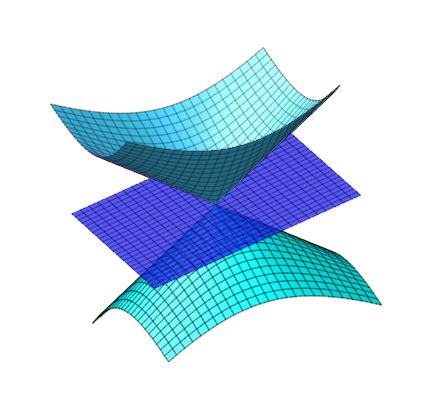
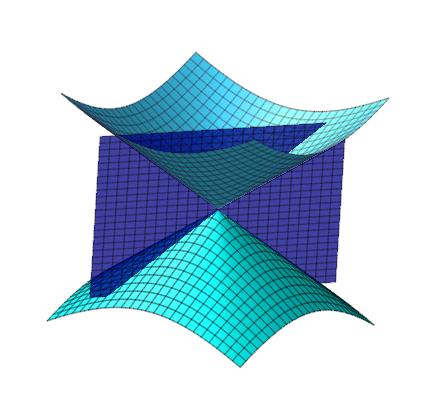
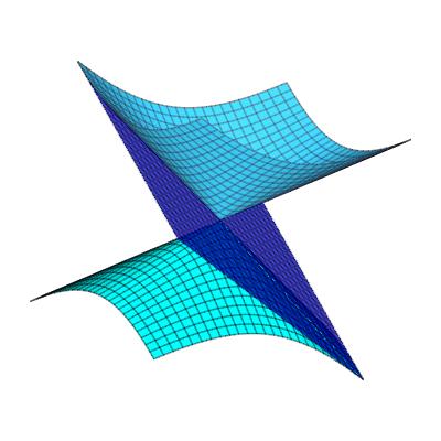
Figure 1: From left to right: a space-, a time- and a lightlike plane in $\mathbb{R}^{3}_{1}$.

We start with an important lemma whose proof is immediate:

Lemma 3.1.

Let $W$ be a subspace of $\mathbb{R}^{n+1}_{1}$.

(a) For any $\gamma\in{\bf O}(n,1)$, $W$ and $\gamma W$ are subspaces of same type (space-, time- or lightlike)

(b) If   $\Sigma_{1},\Sigma_{2}<{\bf O}(n,1)$ are conjugate subgroups, namely $\Sigma_{2}=\gamma^{-1}\Sigma_{1}\gamma$, then $W$ is $\Sigma_{1}$-invariant if, and only if, $\gamma W$ is $\Sigma_{2}$-invariant.

A subspace is nondegenerate if the pseudo inner product restricted to it is a nondegenerate bilinear form. It is well-known that $W$ is nondegenerate if, and only if, $W\cap W^{\perp}$ is trivial (see [17]). We show that an invariant subspace admits $W^{\perp}$ as invariant orthogonal complement if, and only if, it is nondegenerate (Proposition 3.2). If the subspace is degenerate (lightlike) we shall see that it still admits a complement, but this is nonorthogonal, and its invariance is attained under a condition imposed on the group (Proposition 3.3).

Proposition 3.2.

For any subspace $W\subseteq\mathbb{R}^{n+1}_{1}$,

• $\dim W+\dim W^{\perp}=n+1$.

• For a group $\Gamma<{\bf O}(n,1)$, $W$ is nondegenerate and $\Gamma$-invariant if, and only if, its orthogonal subspace is a $\Gamma$-invariant complement, namely $W\oplus W^{\perp}=\mathbb{R}^{n+1}_{1}$.

Proof.

• Consider an operator $\varphi:\mathbb{R}^{n+1}_{1}\to\mathbb{R}^{n+1}_{1}$, $\varphi(x)=AJx$, where $A$ is a square matrix whose lines are formed by basic vectors of $W$ and by lines with all entries equal to 0. We have that $\dim Im\varphi=rank(A)=\dim W$. Thus, $\dim\ker\varphi+\dim W=n+1$. But $\ker\varphi=W^{\perp}$, so the result follows.

• The "if" part is immediate: for $u\in W^{\perp}$ and $\gamma\in\Gamma$, from the $\Gamma$-invariance of $W$, for all $w\in W$ we have

  $$\left<w,\gamma u\right>=\left<\gamma^{-1}w,u\right>=0.$$

  Now, $W$ is nondegenerate if, and only if, $W\cap W^{\perp}$ is trivial which, together with (a), gives the result.

∎

Proposition 3.3.

Let $\Gamma<{\bf O}(n,1)$ such that $\gamma^{t}\in\Gamma$, for all $\gamma\in\Gamma$. If $W$ is a $\Gamma$-invariant lightlike subspace, then $JW^{\perp}$ is a $\Gamma$-invariant complement of $W$, with $W\oplus JW^{\perp}=\mathbb{R}^{n+1}_{1}$.

Proof.

First, notice that $JW^{\perp}$ is $\Gamma$-invariant: for $u=Jv\in JW^{\perp}$,

$$\gamma u=\gamma Jv=J(\gamma^{t})^{-1}v,$$

which belongs to $JW^{\perp}$, since $W^{\perp}$ is $\Gamma$-invariant and $\gamma^{t}\in\Gamma$ by hypothesis. Also, if $w=Jv\in W\cap JW^{\perp}$, then $\left<w,v\right>=0$, and so $\left<Jv,v\right>=0$, implying that $v=0$. Hence, $W\cap JW^{\perp}$ is trivial, Now, it follows from (a) of Proposition 3.2 that $\dim W+\dim(JW^{\perp})=n+1$. Therefore, $W\oplus JW^{\perp}=\mathbb{R}^{n+1}_{1}$. ∎

The two propositions above provide the general way to decompose $\mathbb{R}^{n+1}_{1}$ as a direct sum of an invariant subspace and its complement, depending on its type: if $U$ is a spacelike or a timelike subspace and $W$ is lightlike subspace, then

$$\mathbb{R}^{n+1}_{1}\ =\ U\oplus U^{\perp}\ =\ W\oplus JW^{\perp}.$$

In presence of symmetries, one important class of invariant subspaces is the class of fixed-point subspace. For a given group $\Gamma<{\bf O}(n,1)$, Recall that the fixed-point subspace of a subgroup $\Sigma<\Gamma$ is the subspace

$${\rm Fix}(\Sigma)=\{v\in V:\sigma v=v,\forall\sigma\in\Sigma\}.$$

There are two basic facts that are the main motivations for the results presented in this section, concerning the applications. First, we recall that for a $\Gamma$-equivariant mapping $g$,

$$g({\rm Fix}(\Sigma))\subset{\rm Fix}(\Sigma).$$ (13)

Also, fixed-point subspaces of conjugate subgroups are related by

$$\gamma{\rm Fix}(\Sigma)\subseteq{\rm Fix}(\gamma\Sigma\gamma^{-1}).$$ (14)

One interest is related to symmetric dynamics: when this is ruled by a $\Gamma$-equivariant mapping $g$ (defining a vector field, for instance), we have that (13) holds for all $\Sigma<\Gamma$. Therefore, these are subspaces on which the dynamics must remain invariant. In another direction, we mention the study of the geometry of surfaces which are given as the inverse image $f^{-1}(c)$,  $c\in\mathbb{R}$, for some $f$ $\Gamma$-invariant function. By construction, the whole group leaves this surface setwise invariant and, in addition, the whole space is foliated by these surfaces in a symmetric way. Now, recall that the normalizer N($\Sigma$) is the symmetry group of the set ${\rm Fix}(\Sigma)$, in the sense that it is the largest subgroup of $\Gamma$ that leaves ${\rm Fix}(\Sigma)$ setwise invariant. Hence, we can use that structure to understand the surface "in peaces" preserving their symmetries, once $\Gamma\backslash$ N($\Sigma$) are the symmetries of $f^{-1}(0)\cap{\rm Fix}(\Sigma)$. It now follows from (14) that each peace can be taken in conjugacy classes of subgroups of $\Gamma$.

Notice that in $\mathbb{R}^{3}_{1}$ the orthogonal subspace to a lightlike line $W$ is a plane tangent to the lightcone which contains $W$. Likewise, if $W$ is a lightlike plane then its orthogonal subspace is a lightlike line contained in $W$. This follows directly from the fact that if $W$ in $\mathbb{R}^{n+1}_{1}$ is lightlike then $\dim W\cap W^{\perp}=1$ (see [13] for example) and also from the fact that $W$ is spacelike if, and only if, $W^{\perp}$ is timelike (see [18] for example).

3.1 Invariant lines in $\mathbb{R}^{2}_{1}$

The standard 2-dimensional representation of the Lorentz group is

$${\bf O}(1,1)={\bf SO}_{0}(1,1)\ \dot{\cup}\ \Lambda^{p}{\bf SO}_{0}(1,1)\ \dot{\cup}\ \Lambda^{t}{\bf SO}_{0}(1,1)\ \dot{\cup}\ -I{\bf SO}_{0}(1,1),$$ (15)

where ${\bf SO}_{0}(1,1)$ is the group of hyperbolic rotations,

$$H_{\theta}:=\left(\begin{array}[]{cc}\cosh\theta&\sinh\theta\\ \sinh\theta&\cosh\theta\end{array}\right),$$ (18)

for $\theta\in{\mathbb{R}}$, and

$$\Lambda^{p}=\left(\begin{array}[]{cc}-1&0\\ 0&1\end{array}\right),\ \ \Lambda^{t}=\left(\begin{array}[]{cc}1&0\\ 0&-1\end{array}\right).$$

• For an arbitrary element in ${\bf SO}_{0}(1,1)$ or in the component $-I{\bf SO}_{0}(1,1)$, it is direct that the invariant lines under this element are the two light lines of the lightcone,

  $$W_{1}=\{(x,y)\in\mathbb{R}^{2}_{1}\ :y=x\},\ \ \ W_{2}=\{(x,y)\in\mathbb{R}^{2}_{1}\ :y=-x\}.$$

  These are degenerate subspaces and one is the complement of the other as in Proposition 3.3. Clearly neither is a fixed-point subspace.

• The invariant lines under each $\Lambda^{p}$ and $\Lambda^{t}$ are the $x$-axis (a space line) and the $y$-axis (a time line), and one is the orthogonal complement of the other. The $x$-axis is ${\rm Fix}({\bf Z}_{2}(\Lambda^{t}))$ and the $y$-axis is ${\rm Fix}({\bf Z}_{2}(\Lambda^{p}))$. Any other involution belongs to one of the other two components of (15) and it is conjugate to either $\Lambda^{p}$, if it is of the form $\Lambda^{p}H_{\theta}$, or to $\Lambda^{t}$, if it is of the form $\Lambda^{t}H_{\theta}$, the conjugacy matrix for both cases being $\gamma=H_{-\theta/2}$. Up to conjugacy, there are therefore only two classes of involutions. For any $\theta\in{\mathbb{R}}$, we can use Lemma 3.1 for this $\gamma$ to obtain explicitly all the invariant lines under the involutions of ${\bf O}(1,1)$.

• Any subgroup $\Sigma$ generated by two or more elements has nontrivial invariant subspaces only if $\Sigma<{\bf SO}_{0}(1,1)\times{\bf Z}_{2}(-I)$, and these are $W_{1}$ and $W_{2}$ above.

In Table 1 we summarize these results. The straight lines in the second column are the lines invariant under the subgroups given in the first colum. Their type is given in the third column and the last column shows their complement subspaces.

Table 1: Invariant subspaces of $\mathbb{R}^{2}_{1}$.

Subgroup of ${\bf O}(1,1)$	Invariant subspaces	Type	Complement subspace
$[H_{\theta}]$	$\begin{array}[]{l}W_{1}=\{(x,y)\in\mathbb{R}^{2}_{1}:y=x\}\\ W_{2}=\{(x,y)\in\mathbb{R}^{2}_{1}:y=-x\}\end{array}$	light	$\begin{array}[]{c}JW_{1}^{\perp}=W_{2}\\ JW_{2}^{\perp}=W_{1}\end{array}$
$[-H_{\theta}]$	$\begin{array}[]{c}W_{1}\\ W_{2}\end{array}$	light	$\begin{array}[]{c}JW_{1}^{\perp}=W_{2}\\ JW_{2}^{\perp}=W_{1}\end{array}$
${\bf Z}_{2}(\Lambda^{t})$	$\begin{array}[]{c}{\rm Fix}({\bf Z}_{2}(\Lambda^{t}))=x{\rm-axis}\\ y{\rm-axis}\end{array}$	$\begin{array}[]{c}{\rm space}\\ {\rm time}\end{array}$	$\begin{array}[]{c}{\rm Fix}({\bf Z}_{2}(\Lambda^{t}))^{\perp}\\ {\rm Fix}({\bf Z}_{2}(\Lambda^{p}))^{\perp}\end{array}$
${\bf Z}_{2}(\Lambda^{p})$	$\begin{array}[]{c}{\rm Fix}({\bf Z}_{2}(\Lambda^{p}))=y{\rm-axis}\\ x{\rm-axis}\end{array}$	$\begin{array}[]{c}{\rm time}\\ {\rm space}\end{array}$	$\begin{array}[]{c}y{\rm-axis}\\ x{\rm-axis}\end{array}$

3.2 Invariant lines and invariant planes in $\mathbb{R}^{3}_{1}$

The standard 3-dimensional representation of the Lorentz group is

$${\bf O}(2,1)={\bf SO}_{0}(2,1)\ \dot{\cup}\ \Lambda^{p}{\bf SO}_{0}(2,1)\ \dot{\cup}\ \Lambda^{t}{\bf SO}_{0}(2,1)\ \dot{\cup}\ \Lambda^{pt}{\bf SO}_{0}(2,1),$$ (19)

where ${\bf SO}_{0}(2,1)$ is the group of hyperbolic rotations $H^{+}$ which, using singular value decomposition ([9]), are written as

$$H^{+}=\left(\begin{array}[]{ccc}\cos\varphi&-\sin\varphi&0\\ \sin\varphi&\cos\varphi&0\\ 0&0&\epsilon\end{array}\right)\left(\begin{array}[]{ccc}1&0&0\\ 0&\cosh\theta&\sinh\theta\\ 0&\sinh\theta&\cosh\theta\end{array}\right)\left(\begin{array}[]{ccc}\cos\phi&-\sin(\phi)&0\\ \sin(\phi)&\cos\phi&0\\ 0&0&1\end{array}\right),$$ (29)

for $\varphi,\theta,\phi\in{\mathbb{R}}$ and $\epsilon=1$, and

$$\Lambda^{p}=\left(\begin{array}[]{ccc}1&0&0\\ 0&-1&0\\ 0&0&1\end{array}\right),\ \ \Lambda^{t}=J.$$ (33)

Matrices in the component $\Lambda^{pt}{\bf SO}_{0}(2,1)$ are of the form

$$H^{-}=\left(\begin{array}[]{ccc}\cos\varphi&\sin\varphi&0\\ \sin\varphi&-\cos\varphi&0\\ 0&0&\epsilon\end{array}\right)\left(\begin{array}[]{ccc}1&0&0\\ 0&\cosh\theta&\sinh\theta\\ 0&\sinh\theta&\epsilon\cosh\theta\end{array}\right)\left(\begin{array}[]{ccc}\cos\phi&-\sin\phi&0\\ \sin(\phi)&\cos\phi&0\\ 0&0&1\end{array}\right),$$ (43)

for $\varphi,\theta,\phi\in{\mathbb{R}}$ and $\epsilon=-1$. Matrices in $\Lambda^{t}{\bf SO}_{0}(2,1)$ are of the form (29) for $\epsilon=-1$ and in $\Lambda^{p}{\bf SO}_{0}(2,1)$ are of the form (43) for $\epsilon=1$.

Below we consider invariant subspaces under an element in each of the connected components of ${\bf O}(2,1)$. We recall that elements in distinct components are not conjugate.

• For $H^{+}\in{\bf SO}_{0}(2,1)$, given in (29) with $\epsilon=1$, if $\varphi+\phi=\pi$ then it is conjugate to $-\Lambda^{t}$, by the conjugacy matrix

  $$\left(\begin{array}[]{ccc}-\cos\phi&-\sin\phi\cosh\theta/2&-\sin\phi\sinh\theta/2\\ \sin\phi&-\cos\phi\cosh\theta/2&-\cos\phi\sinh\theta/2\\ 0&\sinh\theta/2&\cosh\theta/2\end{array}\right).$$ (47)

  The invariant lines under $-\Lambda^{t}$ are the time line given by the $z$-axis, which is Fix(${\bf Z}_{2}(-\Lambda^{t})$), and the space lines in the plane $z=0$. The invariant planes are the space plane $z=0$ and all the time planes containing the $z$-axis.

• For $H^{+}\in{\bf SO}_{0}(2,1)$ given in (29) with $\epsilon=1$, if $\varphi+\phi\neq\pi$, invariant lines and planes can be of any type, depending on the values of $\varphi,\theta,\phi$. The subgroup $[H^{+}]$ generated by $H^{+}$ is noncompact, and Fix($[H^{+}]$) is the line generated by the vector

  $$\Bigl{(}1,\frac{\sin\varphi-\sin\phi}{\cos\phi+\cos\varphi},\frac{(\cos\varphi\sin\phi+\sin\varphi\cos\phi\sinh\theta}{(1-\cosh\theta)(\cos\phi+\cos\varphi)}\Bigr{)},$$

  which can also be of any type.

• For $\Lambda^{t}H^{+}\in\Lambda^{t}{\bf SO}_{0}(2,1)$, given in (29) with $\epsilon=-1$, if $\varphi=-\phi$ then it is conjugate to $\Lambda^{t}$, by the conjugacy matrix (47). The invariant lines under $\Lambda^{t}$ are the time line given by the $z$-axis, and the space lines in the plane $z=0$. The invariant planes are the space plane $z=0$ which is Fix(${\bf Z}_{2}(\Lambda^{t})$) and all the time planes containing the $z$-axis.

• For $\Lambda^{t}H^{+}\in\Lambda^{t}{\bf SO}_{0}(2,1)$ given in (29) with $\epsilon=-1$ and for $\varphi\neq\phi$, Fix(${\bf Z}_{2}(\Lambda^{t}H^{+})$) is trivial. There are no invariant lines or planes by the action of the group ${\bf Z}_{2}(\Lambda^{t}H^{+})$.

• For $\Lambda^{p}H^{-}\in\Lambda^{p}{\bf SO}_{0}(2,1)$, given in (43) with $\epsilon=1$, if $\varphi=-\phi$ then it is conjugate to $\Lambda^{p}$, by the conjugacy matrix (47). The invariant lines under $\Lambda^{p}$ are the space line given by the $y$-axis, and the time lines in the plane $y=0$. AQUI The invariant planes are the time plane $y=0$ which is Fix(${\bf Z}_{2}(\Lambda^{p})$) and all the time planes containing the $y$-axis.

• For $\Lambda^{p}H^{-}\in\Lambda^{p}{\bf SO}_{0}(2,1)$ given in (29) with $\epsilon=1$, if $\varphi\neq\phi$ then Fix(${\bf Z}_{2}(\Lambda^{p}H^{+})$) is trivial. There are no invariant lines or planes by the action of the group ${\bf Z}_{2}(\Lambda^{p}H^{-})$.

• For $H^{-}\in\Lambda^{pt}{\bf SO}_{0}(2,1)$, given in (43) with $\epsilon=-1$, if $\varphi+\phi=\pi$ then it is conjugate to $-\Lambda^{p}$, by the conjugacy matrix (47). The invariant lines under $-\Lambda^{p}$ are the space line given by the $y$-axis, which is Fix(${\bf Z}_{2}(-\Lambda^{p})$), and the all lines in the plane $y=0$, whose types are time-, light- and spacelike. The invariant planes are the time plane $y=0$ and all the planes containing the $y$-axis, which are the two light planes $z\pm x=0$ (tangent to the lightcone) and all space and time planes containing the $y$-axis.

• For $H^{-}\in\Lambda^{pt}{\bf SO}_{0}(2,1)$, given in (43) with $\epsilon=-1$, if $\varphi+\phi\neq\pi$, invariant lines and planes can be of any type, depending on the values of $\varphi,\theta,\phi$. The subgroup $[\Lambda^{pt}H^{+}]$ generated by $\Lambda^{pt}H^{+}$ is noncompact, and Fix($[\Lambda^{pt}H^{+}]$) is the line generated by

  $$\Bigl{(}1,-\frac{\sin(\phi)-\sin(\varphi)}{\cos\phi+\cos\varphi},-\frac{(\cos\varphi\sin(\phi)+\sin(\varphi)\cos\phi)\sinh\theta}{(\cosh\theta+1)(\cos\phi+\cos\varphi)}\Bigr{)}$$

  which can also be of any type.

Finally, if a subgroup $\Sigma<{\bf O}(2,1)$ is generated by more than one element, then these appear in the list above and so Fix($\Sigma$) is computed directly as the intersection of the fixed-point subspaces of each of its generators.

Acknowledgments. The authors acknowledge partial support by CAPES under CAPES/FCT grant 99999.008523/2014-02 and CAPES/PROEX grant 1183747.

References

• [1] Antoneli, F.; Baptistelli, P.H.; Dias, A. Manoel, M. Invariant theory and reversible-equivariant vector fields. J. Pure Appl. Algebra 213 (2009), no. 5, 649–663. MR2494358 (2010h:37114)
• [2] Baptistelli, P.H.; Manoel, M. Relative equivariants under compact Lie groups. Top. its Appl. 234 (2018), 474–487.
• [3] Baptistelli, P.H.; Manoel, M. Invariants and relative invariants under compact Lie groups. J. Pure Appl. Algebra 217 (2013), no. 12, 2213–2220.
• [4] Baptistelli, P.H.; Manoel, M. The $\sigma$-isotypic decomposition and the $\sigma$-index of reversible-equivariant systems. Topology Appl. 159 (2012), no. 2, 389–396.
• [5] Bayrakdar, T., Ergin, A. A. Time-like Hamiltonian dynamical sustems in Minkowski space $\mathbb{R}^{3}_{1}$ and the nonlinear evolution equations. Mathematicki Vesnik 70, no. 1, 12–25.
• [6] Brown, H.R., Read, J. The dynamical approach to spacetime theories. Faculty of Philosophy, University of Oxford, preprint (2018).
• [7] Buono, P-L.; Lamb, J.S.W.; Roberts, M. Bifurcation and branching of equilibria in re-equivariant vector fields. Nonlinearity 21, no. 4, (2008), 625–660.
• [8] Chossat, P.; Lauterbach, Reiner. Methods in equivariant bifurcations and dynamical systems. Advanced Series in Nonlinear Dynamics, 15. World Scientific Publishing Co., Inc., River Edge, NJ, 2000. xvi+404 pp. ISBN: 981-02-3828-2.
• [9] Gallier, J. Notes on group actions, manifolds, Lie groups, and Lie algebras. University of Pennsylvania, 27 (2005).
• [10] Gatermann, K. Computer algebra methods for equivariant dynamical systems. Lecture Notes in Mathematics, 1728. Springer-Verlag, Berlin, 2000. xvi+153 pp. ISBN: 3-540-67161-7.
• [11] Gatermann, K. Semi-invariants, equivariants and algorithms. Appl. Algebra Engrg. Comm. Comput. 7 (1996), no. 2, 105–124.
• [12] Golubitsky, M., Stewart, I., Schaeffer, D. Singularities and groups in bifurcation theory. Vol. II. Applied Mathematical Sciences, 69. Springer-Verlag, New York, 1988. xvi+533 pp. ISBN: 0-387-96652-8.
• [13] Izumiya, S. Legendrian dualities and spacelike hypersurfaces in the lightcone, Mosc. Math. J. 9 (2009) no. 2, 325–357.
• [14] Janssen, M. Drawing the Line Between Kinematics and Dynamics in Special Relativity, Stud Hist. Phil. Mod. Phys., 40 (2009), 26–52.
• [15] Lamb, J. S. W., Roberts, M. Reversible equivariant linear systems. J. Differential Equations 159 (1999), no. 1, 239–279.
• [16] Manoel, M., Roberts, M. Gradient systems on coupled cell networks. Nonlinearity 28 (10) (2015) 3487–3509.
• [17] O’neill, B. Semi-Riemannian geometry with applications to relativity, Academic Press 103) (1983).
• [18] Ratcliffe, J. Foundations of hyperbolic manifolds, Springer Science & Business Media 149 (2006).
• [19] Stewart, I., Golubitsky, M., Pivato, M. Symmetry groupoids and patterns of synchrony in coupled cell networks. SIAM J. Appl. Dyn. Syst. 2 (2003), no. 4, 609–646.
• [20] Sturmfels, B. Algorithms in invariant theory. Texts and Monographs in Symbolic Computation, Springer-Verlag, Vienna, 1993. vi+197 pp. ISBN: 3-211-82445-6.