Sub-GeV Dark Matter Searches and Electric Field Studies for the LUX and LZ Experiments

Abstract

Abundant evidence from cosmological and astrophysical observations suggests that the Standard Model does not describe 84% of the matter in our universe. The nature of this dark matter (DM) remains a mystery since it has so far eluded detection in the laboratory. To that end, the Large Underground Xenon (LUX) experiment was built to directly observe the interaction of DM with xenon target nuclei. LUX acquired data from April 2013 to May 2016 at the Sanford Underground Research Facility (SURF) in Lead, South Dakota, which led to publications of many world-leading exclusion limits that probe much of the unexplored DM parameter space.

This manuscript describes two novel direct detection methods that used the first LUX dataset to place limits on sub-GeV DM. The Bremsstrahlung and Migdal effects consider electron recoils that accompany the standard DM-nucleus scattering, thereby extending the reach of the LUX detector to lower DM masses. The spin-independent DM-nucleon scattering was constrained for four different classes of mediators for DM particles with masses of 0.4-5 GeV/c².

The detector conditions changed significantly before its final 332 live-days of data acquisition. The electric fields varied in a non-trivial non-symmetric manner, which triggered a need for a fully 3D model of the electric fields inside the LUX detector. The successful modeling of these electric fields, described herein, enabled a thorough understanding of the detector throughout its scientific program and strengthened its sensitivity to DM.

The LUX-ZEPLIN (LZ) experiment, the successor to LUX, is a next-generation xenon detector soon to start searching for DM. However, increasingly large noble liquid detectors like LZ are facing challenges with applications of high voltage (HV). The Xenon Breakdown Apparatus (XeBrA) at the Lawrence Berkeley National Laboratory was built to characterize the HV behavior of liquid xenon and liquid argon. Results from XeBrA will serve not only to improve our understanding of the physical processes involved in the breakdown but also to inform the future of noble liquid detector engineering.

2019

Chapter 1 Quest for the missing mass

The missing mass in our universe is one of the critical mysteries of contemporary physics. Despite the success of the Standard Model (SM) of particle physics developed in the 1970’s, the nature of 84% of the matter remains a mystery. The existence of dark matter (DM) was first postulated in 1933 by Fritz Zwicky [1] to account for the missing mass in orbital velocities of galaxy clusters. A satisfactory explanation of this missing matter requires the existence of a “dark” particle lacking electromagnetic interactions. Nowadays, DM enjoys plenty of attention from both theoretical and experimental physicists. There is abundant evidence for DM from cosmological and astrophysical observations, but it keeps eluding detection, which is the focus of this dissertation.

This chapter first presents an overview of the evidence supporting the existence of dark matter, along with DM candidates, and the possible detection methods with a focus on direct detection. The remainder of this work then discusses techniques developed in support of the quest for dark matter.

1.1 Evidence for dark matter

The amount of observational evidence for the existence of DM has steadily increased over the last several decades. This section reviews observational studies of the composition of our universe pointing toward the evidence of dark matter. The evidence comes at various scales: cosmological (Section 1.1.1), the scale of clusters (Section 1.1.2), or at the local galactic scale (Section 1.1.3).

1.1.1 Cosmological scale

The standard Big Bang model is based on three fundamental astronomical observations: the homogeneity and isotropy of the universe on large scales, the blackbody spectrum of the cosmic microwave background (CMB) radiation and the Hubble law. Based on those observations, the Friedmann-Lemaitre-Robertson-Walker (FLRW) metric can be used to describe our universe in comoving spherical coordinates $\left(r,\theta,\phi\right)$:

$$ds^{2}=dt^{2}-a^{2}(t)\left[\frac{dr^{2}}{1-kr^{2}}+r^{2}(d\theta^{2}+\sin^{2}\theta d\phi^{2})\right]$$ (1.1)

where $a(t)$ is a scale factor that represents the time-dependent expansion of the universe and relates the changing proper distance $d(t)$ between a pair of objects

$$d(t)=a(t)d_{0}$$ (1.2)

where $d_{0}$ is the distance at a reference time $t_{0}$. By definition $a(t_{0})=1$ at present time $t=t_{0}$. Different geometries of space are described by the constant $k$, with $k=1$ for elliptical, $k=0$ for Euclidean, and $k=-1$ for hyperbolic space. The measurement and description of those two quantities, $k$ and $a$, is the main focus of cosmology.

Combining the FLRW metric in Equation 1.1 and Einstein’s field equations yields an equation for the Hubble parameter, defined as the rate of change of the scale factor with time:

$$H\left(t\right)^{2} \equiv\left(\frac{\dot{a}\left(t\right)}{a\left(t\right)}\right)^{2}$$ (1.3)

$$=\frac{8\pi G_{N}}{3}\rho-\frac{k}{a^{2}}$$ (1.4)

where $G_{N}$ is the Newton gravitational constant, and $H$ is the Hubble parameter. This equation depends linearly on

$$\rho=\rho_{M}+\rho_{R}+\rho_{\Lambda}$$ (1.5)

which is the average density of the universe with contributions from matter $\rho_{M}$, radiation $\rho_{R}$, and the cosmological constant $\rho_{\Lambda}$, the value of the energy density of the vacuum of space. The total energy density evolves as a function of $a$ and can be found by solving the equation of state of the fluid filling the universe $P=P(\rho)$:

$$\frac{d(\rho a^{3})}{da}=-3Pa^{2}.$$ (1.6)

This results in $\rho_{M}\propto a^{-3}$ for matter, $\rho_{R}\propto a^{-4}$ for radiation, and $\rho_{\Lambda}\propto\mathrm{const}.$ for cosmological constant.

The observation of redshifts of Type Ia supernovae (SNe) at large distances in 1998 [4, 5] found evidence for an accelerating universe caused by a dark energy component. Furthermore, since the path of light depends on the curvature of the universe, analysis of the CMB discovered that $k$ is very close to 0, consistent with a flat universe. Therefore, using Equation 1.4 we can define a critical density $\rho_{cr}$. The results of this theoretical framework combined with observations can be used to calculate the critical density

$$\rho_{cr} =\frac{3H_{0}^{2}}{8\pi G_{N}}$$ (1.7)

$$\equiv\frac{\rho}{\Omega}.$$ (1.8)

which is estimated to be about five atoms of monatomic hydrogen per cubic meter. Here $\Omega$ is the energy density in units of the critical density with

$$\Omega=\sum_{i}\Omega_{i}$$ (1.9)

where the sum is over all the different species of material in the universe (baryonic matter, dark matter, radiation and cosmological constant $\Lambda$), and $\Omega=1$ is equivalent to a flat universe with $k=0$ [6]. By comparing observations and calculations for the constituent parts of $\Omega$, we can conclude that the universe today is most likely dominated by cold particles, i.e., those that had non-relativistic velocities when they decoupled from the thermal plasma after Big Bang [7, 8, 9]. This theoretical framework, known as “Lambda Cold Dark Matter” ($\Lambda$CDM) model is the cosmological equivalent of the Standard Model of particle physics, which enables us to place constraints on the dark matter density.

There is a wealth of evidence from cosmology and astronomy that can be used to constrain the amount of dark matter in the universe [10, 11]; the remainder of this section highlights some of the methods used to place constraints on the amount of dark matter in the universe.

1.1.1.1 The cosmic microwave background

The most powerful constraints on the free parameters in $\Lambda$CDM come from the CMB, which originates from background radiation of decoupled photons in the early universe. CMB has a blackbody spectrum [12] with $T=2.726\,\mathrm{K}$ and is known to be isotropic at $10^{-5}$ level [13]. The small anisotropies $\Delta T/T$ shown in Figure 1.2 can be used to constrain cosmological parameters as shown in Figure 1.2. Since the CMB blackbody spectrum peaks at $\lambda\sim 2\,\mathrm{mm}$, a wavelength readily absorbed by water molecules in the atmosphere, it is studied using satellite missions such as COBE, WMAP, or Planck.

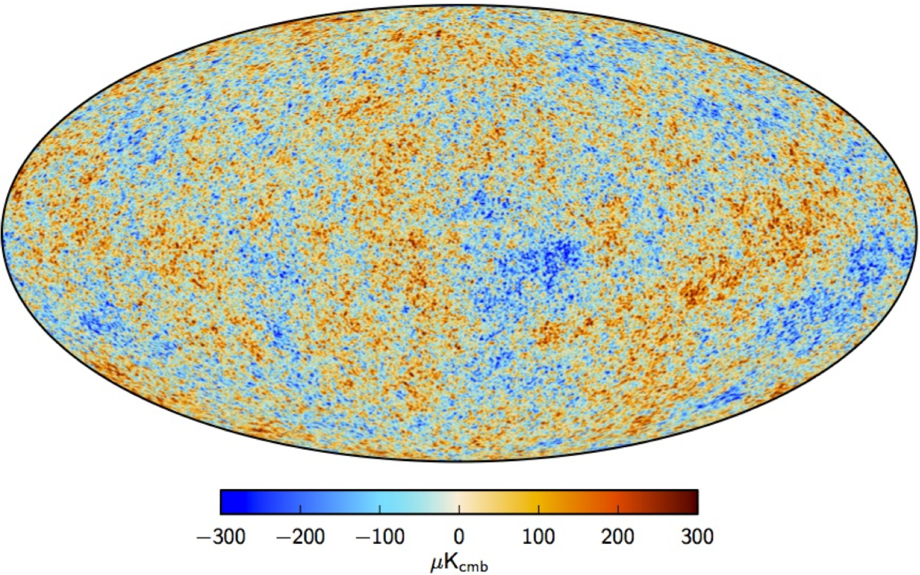
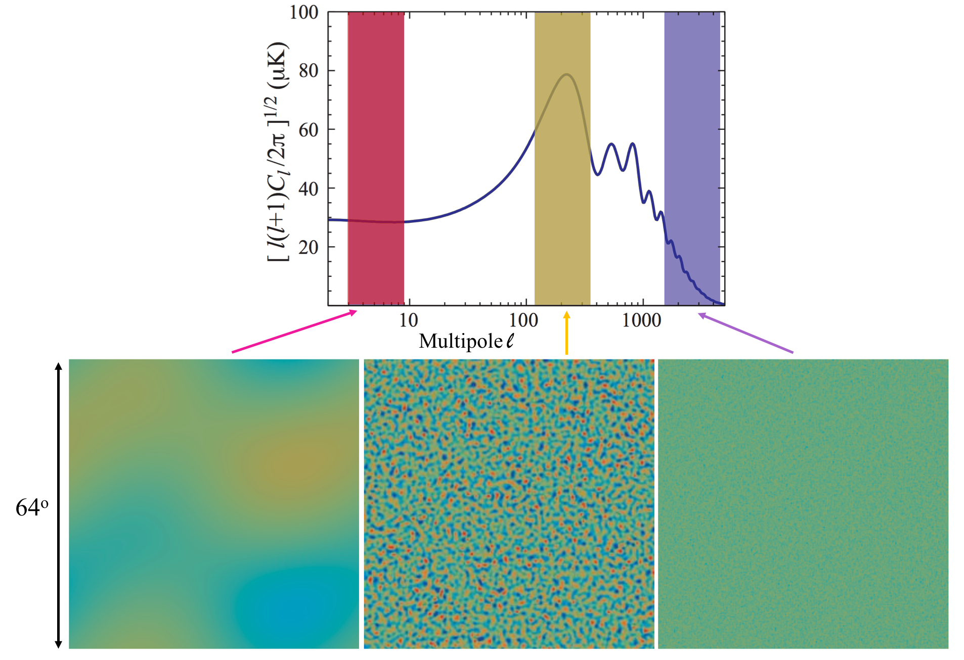
Figure 1.1: A map of the temperature fluctuations of the CMB as seen by the Planck Satellite. Figure from [14].

Figure 1.2: From temperature fluctuations to the power spectrum. A band filter was applied to a temperature fluctuation map (such as the one shown in Figure 1.2) to illustrate the power spectrum at three different regimes. This figure was made using simulations. Figure modified from [15].

The temperature map can be expanded using spherical harmonics $Y_{lm}(\theta,\phi)$. On small scales where the curvature of space can be neglected, a Fourier analysis can be performed and the spherical harmonics $l$ become the Fourier wavenumbers. The power spectrum can be fitted as shown in Figure 1.4 and characterized as a function of the multipole number $l$. The angular wavelength $\theta=2\pi/l$, so large multipole moments $l\sim 10^{2}$ correspond to a few degrees of separation on the sky. The precise location of each peak is sensitive to different parameters of the cosmological model as illustrated in Figure 1.4.

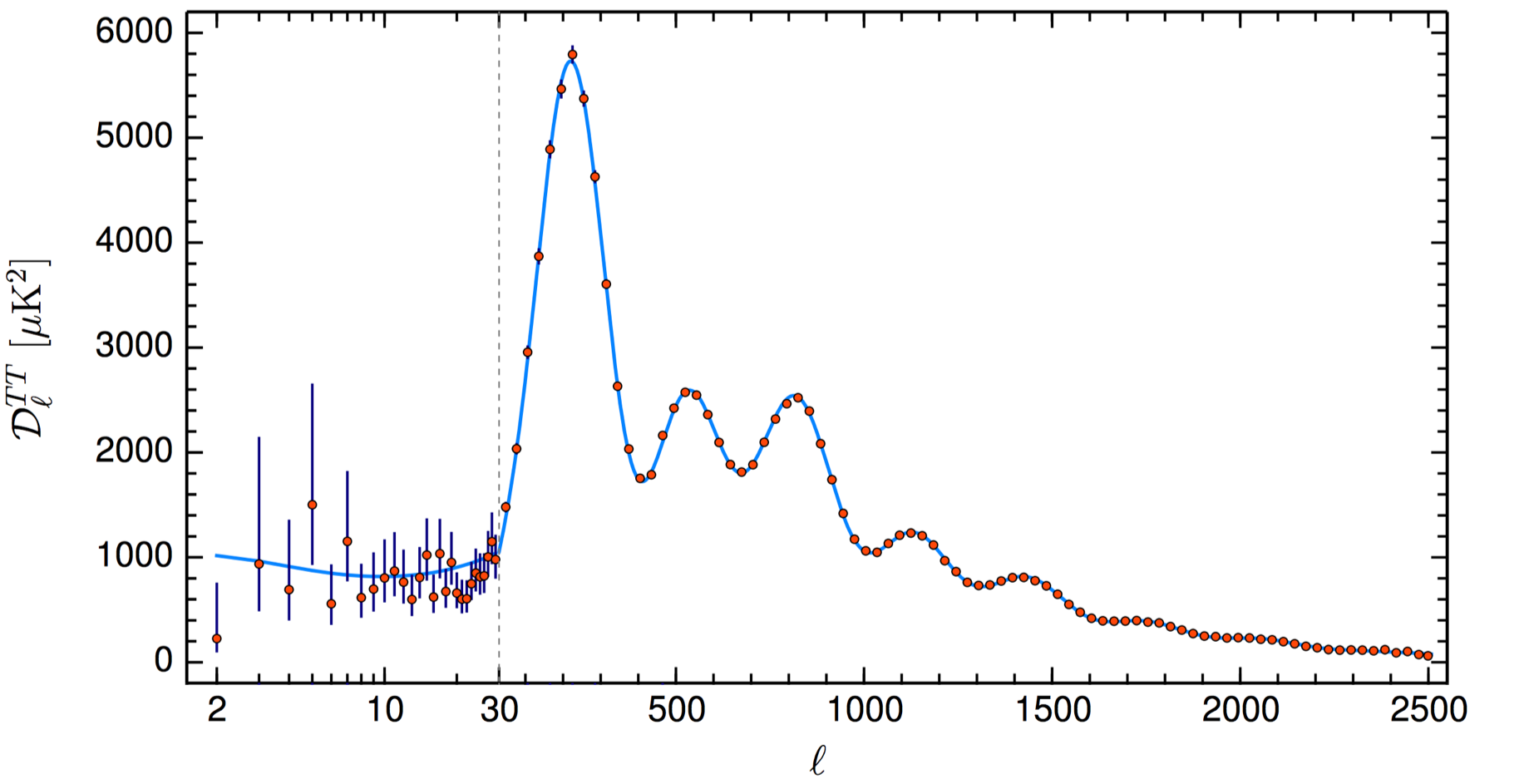
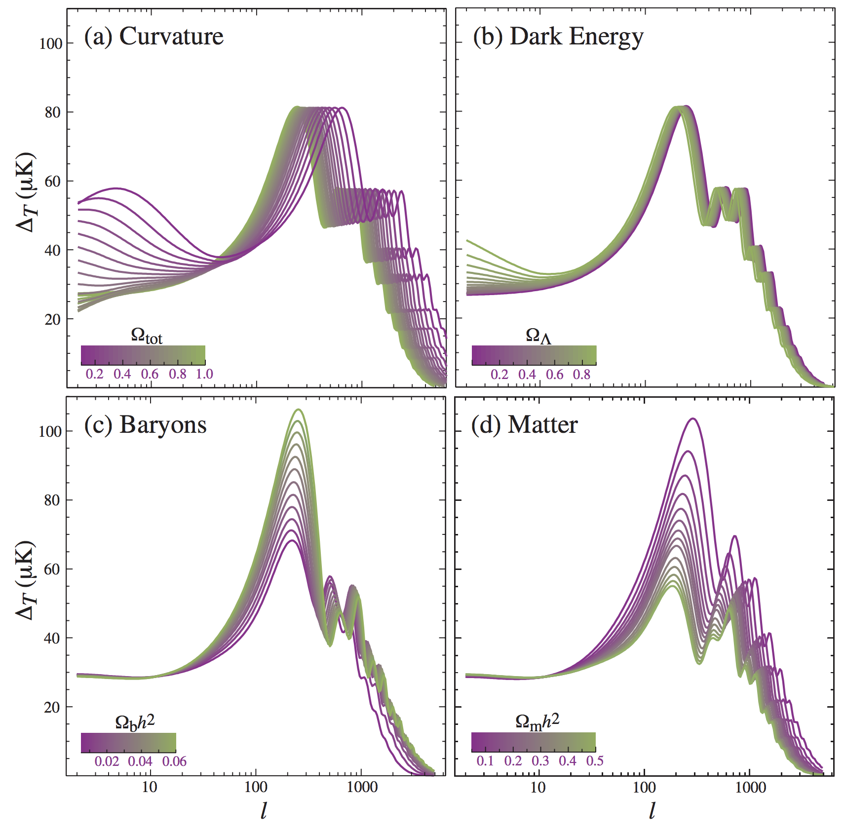
Figure 1.3: The temperature power spectrum measured by Planck (red dots). The solid blue line shows the prediction from the best-fit ΛCDM theoretical spectrum. The vertical gray dashed line indicates a scale change on the horizontal axis from logarithmic to linear. The location of the first peak gives information about the total amount of matter in the universe, which is dependent on the speed of sound of the photon-baryon fluid before decoupling, while the second peak provides information about the total amount of baryonic matter in the universe. Figure from [16].

Figure 1.4: The sensitivity of the acoustic temperature spectrum to a) the curvature $k$, b) the dark energy $\Omega_{\Lambda}$, c) the baryon density $\Omega_{b}$, and d) the matter density $\Omega_{m}$. Models were varied around $\Omega_{tot}=1$. Figure from [17].

By combining the results of the best fit values from the CMB, along with many of the observations described below, the Planck collaboration constrained the main parameters of the $\Lambda$CDM model. The resulting values of the different density components in our universe are presented in Table 1.1.

Parameter	Symbol	Value
Baryonic matter density	$\Omega_{b}$	$0.0490\pm 0.0003$
Cold dark matter density	$\Omega_{c}$	$0.2606\pm 0.0020$
Total matter density	$\Omega_{m}=\Omega_{b}+\Omega_{c}$	$0.3111\pm 0.0056$
Dark energy density	$\Omega_{\Lambda}$	$0.6889\pm 0.0056$

Table 1.1: Selected constraints on the density parameters in the $\Lambda$CDM model as reported by the Planck collaboration [16]. Note that some of those are derived quantities, rather than direct parameters of the model. Uncertainties are given at the 68% interval.

1.1.1.2 Baryon acoustic oscillations

Acoustic oscillations of the baryon-photon fluid from the pre-recombination fluid are imprinted in the large-scale structures of the universe. These oscillations provide a standard length scale by looking at the correlation between large-scale objects. After inflation, higher dark matter density regions attracted matter, which started forming structures by gravitationally attracting surrounding matter. As the baryon density increased, the increase of radiation pressure resulted in acoustic waves, which propagated until decoupling. This created hotter regions where matter contracted, and cooler regions, which resulted in photon emission. Between the formation of those perturbations and the epoch of recombination, the sound waves with different wavelengths will complete a different number of oscillations. This translates time into a characteristic length scale: the maximum distance that an acoustic wave traveled before the epoch of recombination provides a “standard ruler” for length scale in cosmology.

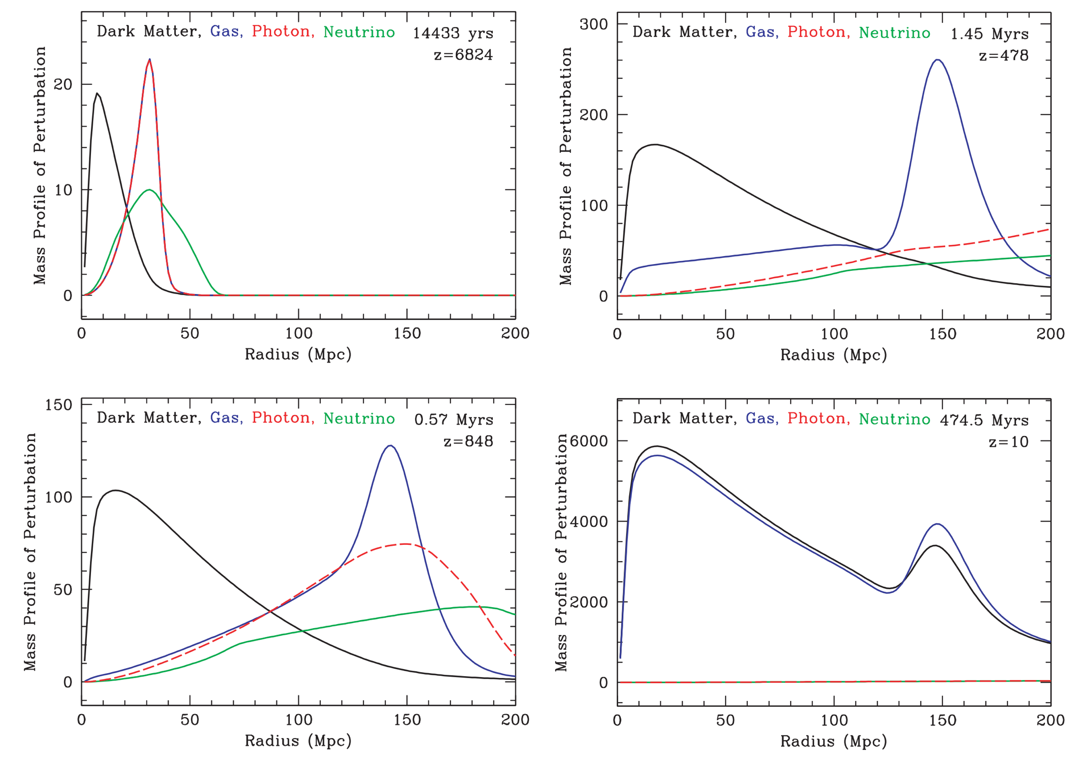
Figure 1.5: Simulated thermal history of the universe with dark matter (black), gas (baryons, blue), and photons (red). An acoustic wave drives photons and baryons together in a tightly bound plasma. After decoupling, photons stream away while the baryon wave stalls at a length scale of 150 Mpc, still visible today. Figure modified from [18].

The baryon acoustic oscillations (BAO) measure the comoving separation of large-scale objects (such as galaxies) at the sound horizon of the time of photon-baryon decoupling. An excess clustering at a particular length scale can then be used to constrain the DM density, as illustrated in Figure 1.5. This effect has been measured using a spectroscopic survey of luminous red galaxies [19] from the Sloan Digital Sky Survey [20]. The shape of the correlation function obtained from the distribution of galaxies in the universe provides a measurement of the matter density $\Omega_{m}$. This constraint from BAO combined with others is shown in Figure 1.6.

1.1.1.3 Big Bang nucleosynthesis

Big Bang nucleosynthesis (BBN) is a sequence of nuclear reactions that led to the synthesis of light elements such as D, ³He, ⁴He, and ⁷Li during the first hundreds of seconds after the Big Bang. Before the epoch of nucleosynthesis, the universe was hot and dense enough for all the particles to be in equilibrium. As the expansion proceeded and temperature decreased some particles were able to separate from the thermodynamic equilibrium with the plasma. First to “freeze out” from the plasma (drop out of thermal equilibrium) were neutrinos at $t\approx 0.1\,\mathrm{s}$ with temperatures $\sim 2-3\,\mathrm{MeV}$ since the neutral current weak interactions became too slow to keep up with the expansion rate. At $t\approx 1\,\mathrm{s}$ with $T\sim 1\,\mathrm{MeV}$ the charged-current weak interactions became too slow to maintain neutron-proton equilibrium and the n/p density ratio froze out at $\mathrm{n/p}\sim 1/7$.

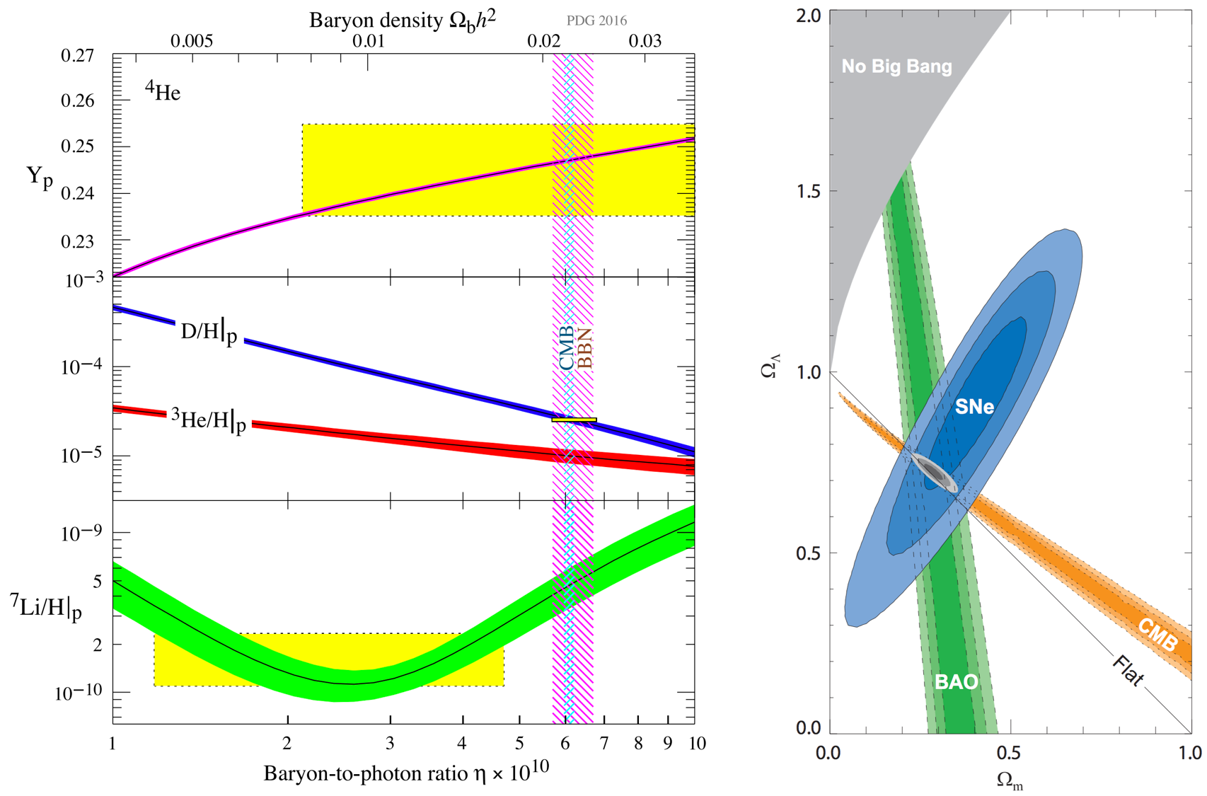
Figure 1.6: Left: The abundances of ⁴He, D, ³He, and ⁷Li as predicted by BBN. The bands show the 95% CL range, boxes indicate the observed light element abundances, and the narrow vertical band is a result from CMB measurements of the cosmic baryon density. The wider band indicates the BBN concordance range. Figure from [21]. Right: Constraints on $\Omega_{m}$ and $\Omega_{\Lambda}$ obtained from CMB, BAO [19], and SNe. The contours show 68.3 %, 95.4 % and 99.7% confidence level. Figure from [22].

At $t\gtrsim 100\,\mathrm{s}$ the universe expanded and cooled enough so that photons were no longer able to photo-dissociate deuterium (D), which marks the start of nucleosynthesis. The formation of D strongly depends on $\eta$, the baryon-to-photon ratio $\eta=\frac{n_{N}}{n_{\gamma}}$ that gives the total number of nucleons, bound or free, as a fraction of photons. BBN eventually stops at $t\gtrsim 1000\,\mathrm{s}$ since the Coulomb barrier becomes too large for nuclear fusion and nucleosynthesis to occur [23].

The baryon-to-photon ratio is also crucial for determining the density of baryons $\Omega_{b}$; the importance of deuterium as a “baryometer” was recognized for the first time in the 1970’s. The equilibrium abundance of D is not well known observationally because it is not clear how much of the dark matter in the universe is in the form of nucleons, but the upper bound to the primordial D abundance can be obtained by measuring the quasar Lyman-$\alpha$ lines to find the baryon density $\Omega_{b}$ [9, 24]. This constrains the number of baryons and hence baryonic DM, implying that the majority of DM must be non-baryonic since $\Omega_{m}\gg\Omega_{b}$.

Figure 1.6 shows the observed and predicted primordial abundances of light elements compared to results from the CMB. The agreement of the two models confirms the success of the $\Lambda$CDM model.

1.1.2 Gravitational lensing

The existence of dark matter can also be inferred from collisions of galaxy clusters. The most famous example of this is the Bullet Cluster 1E0657−558. Gravitational lensing leverages the fact that massive objects in the foreground bend light from a bright, distant source. A particular type of gravitational lensing, known as weak lensing, determines the presence of an intermediate mass through correlations in the observed ellipticity of the distorted objects. This method was used to measure the distribution of mass in the Bullet Cluster, shown as green outlines in Figure 1.7. Along with the images from the Hubble Space Telescope used for the weak lensing measurements, researchers analyzed the x-ray spectra of the cluster recorded by the Chandra X-ray Observatory. The inferred mass from those two techniques produced disparate results. It implies that the x-ray emitting ordinary matter clustered together in the center during the collision, while the two cores of the galaxies passed through one another with little interaction, suggesting that weakly-interacting dark matter forms the majority of the cluster’s mass.

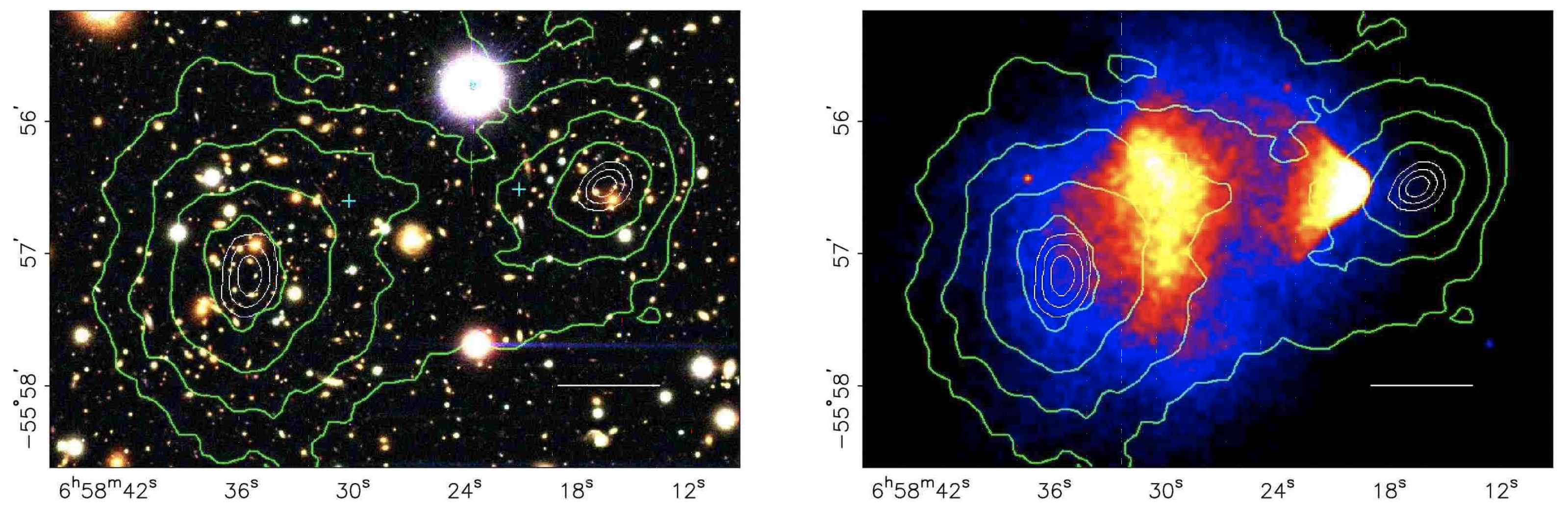
Figure 1.7: Two images of the merging cluster 1E0657−558, known as Bullet cluster, from the Hubble Space Telescope (left), illustrating the distribution of galaxies, and from the Chandra X-ray Observatory (right), illustrating the intracluster plasma. The green contours show the reconstructed mass from weak gravitational lensing. The white bar indicates 200 kpc. Figures from [28].

There are now many examples of non-gravitational interactions of dark matter in colliding galaxy clusters. In 2015, Reference [29] examined 72 collisions using the Chandra and Hubble Space Telescopes. The observed offset of the center of mass for the gas and stars from the DM confirmed the existence of DM at 7.6$\sigma$ significance.

1.1.3 Rotational velocity of spiral galaxies

Further evidence for DM comes from observations. Fritz Zwicky was the first to infer the existence of dark matter from measurements of the velocity dispersion of galaxies in the Coma cluster. By applying the virial theorem to the gravitational potential $U$ and rotational kinetic energy $\left\langle T\right\rangle=-\frac{1}{2}\left\langle U\right\rangle$, he found that the mass-to-light ratio significantly outweighed the mass deduced from the system’s luminosity.

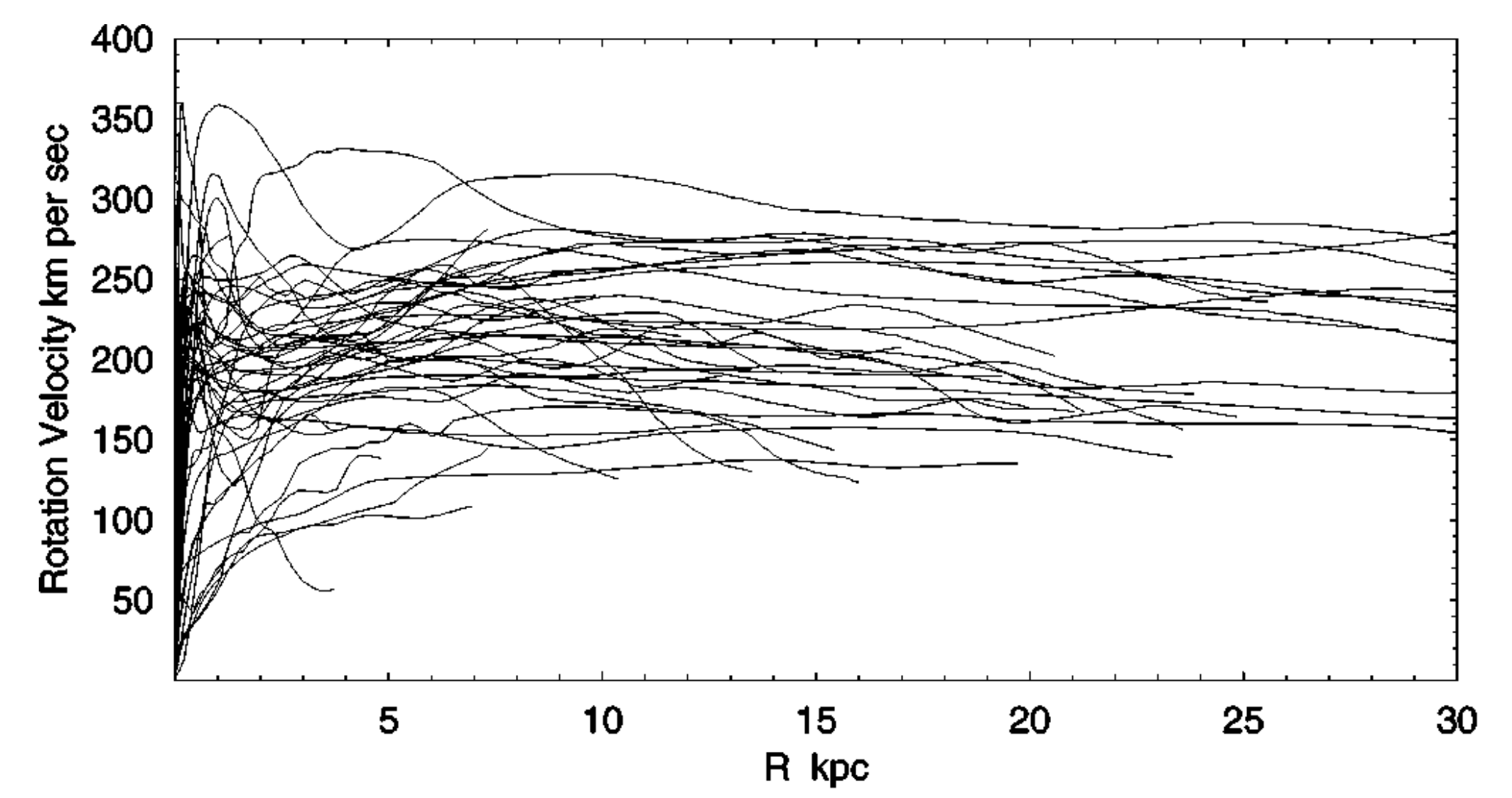
Figure 1.8: A compilation of rotation curves of spiral galaxies from various sources. The flatness of the curves at large radii indicates the presence of a DM halo. Figure from [30].

Another piece of evidence came much later, in the 1970’s-1980’s from observations of galactic rotation curves by V. Rubin et al. [31]. The rotational velocity $v$ of a point-like object on a Keplerian orbit with radius $r$ around a galaxy should follow the equation

$$v(r) =\sqrt{\frac{GM(r)}{r}}$$ (1.10)

derived from Newton’s second law, where $G$ is the gravitational constant and $M$ is the reduced mass. However, the observed velocity outside the visible part of the galaxies does not decline as predicted by the equation but becomes approximately constant as shown in Figure 1.8, which compiles rotation curves from many galaxies. This suggests the existence of a DM halo with mass density $\rho(r)\propto 1/r^{2}$ and $M(r)\propto r$ and gives a lower bound to the DM mass density $\Omega_{DM}\gtrsim 0.1$ [32]. Note that $\rho$ needs to fall faster at some radius, but when this happens is as yet unknown.

1.2 Dark matter candidates

There is a plethora of DM candidate particles, and finding a suitable candidate requires physics beyond the SM. Since $\Omega_{m}\gg\Omega_{b}$ this suggests that most matter in the universe must be non-baryonic, candidates for DM particles must be stable on cosmological scales, interact only weakly (or not at all) with electromagnetic radiation, and be non-relativistic at the time of freeze-out, or “cold.” Such candidates include, for example, primordial black holes, Weakly Interacting Massive Particles (WIMPs), Strongly Interacting Massive Particles (SIMPs), axions, or hidden DM. Constraints on DM are usually calculated assuming that a single species constitutes all of DM, but it is possible that a combination of these candidates is responsible for $\Omega_{c}$. Reviews of possible DM candidates can be found, for example, in [33, 34, 35]. Below we focus on the WIMP and the axion, two of the more popular candidate particles.

1.2.1 Axions

Axions are motivated by the fact that the violation of the charge conjugation parity (CP) symmetry has not been observed in strong interactions in quantum chromodynamics (QCD). The solution from Peccei and Quinn (PQ) [36] introduces a pseudoscalar field $a$ where the particle associated with the symmetry breaking is the axion [37, 38]. Axion is an extremely light, weakly interacting particle produced non-thermally that can also serve as a well-motivated dark matter candidate. Several constraints bound the axion mass $m_{a}$; the most stringent limit derived from the observed length of the neutrino pulse from Supernova 1987a requires $m_{a}\lesssim 10\,\mathrm{meV}$ [39].

Various experiments are searching for axions both directly and indirectly as illustrated in Figure 1.9. Axions are theorized to interact with gluons, fermions, and photons. However, most experiments search for axions through the Primakoff effect where a pseudoscalar is converted into a photon in the presence of an electromagnetic field [40] with a coupling strength given by $g_{a\gamma\gamma}$. The resulting photon is collinear with the incoming axion, and the photon’s energy is equal to the axion’s total energy in a time-independent magnetic field. Direct experiments use for example haloscopes [41, 42] to search for a resonant radio frequency corresponding to the Compton wavelength of the axion or helioscopes which use a strong magnetic field to convert axions produced in the Sun into x-rays [43]. Indirect astrophysical and cosmological searches consider stellar evolutions to place upper bounds on the axion coupling.

While axions remain to be observed directly, their theoretical motivation for resolving the CP problem while serving as an attractive DM particle makes them an attractive candidate for both contemporary and planned searches. For a more in-depth review of axions consult for example [44, 45].

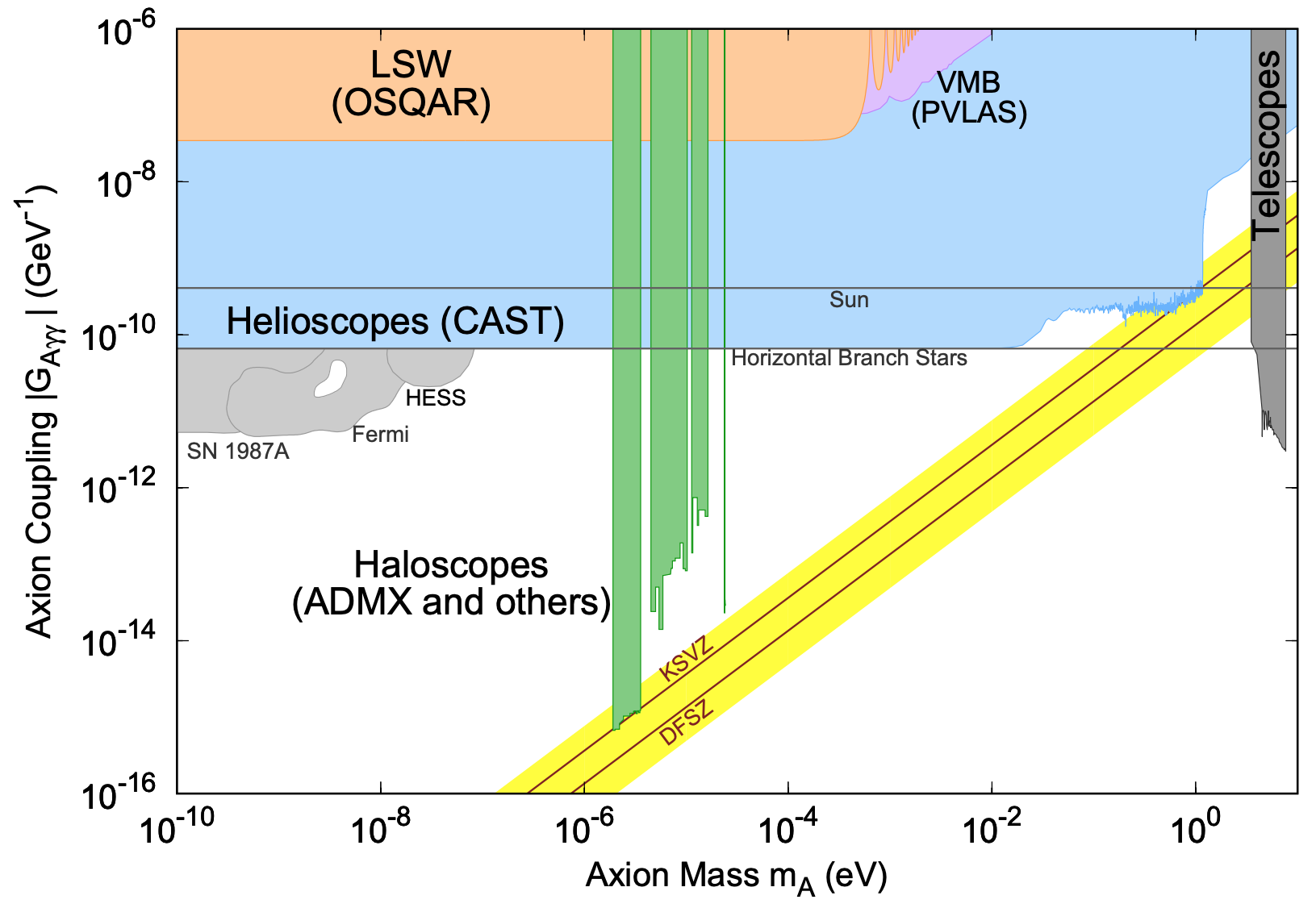
Figure 1.9: Exclusion plot from axion searches. KSVZ [46] and DFSZ [47] refer to archetype theoretical predictions for axion coupling models. LSW refers to the current leading limit from a “light shining through walls” experiment [48] while VMB stands for vacuum magnetic birefringence looking for a change in the polarization of light caused by the Primakoff effect [49]. Figure from [21].

1.2.2 WIMPs

WIMPs ($\chi$) are non-relativistic particles with an expected mass between $\mathrm{GeV/c^{2}-100\,\mathrm{TeV/c^{2}}}$. Their present relic density can be calculated assuming that WIMPs were in thermal and chemical equilibrium with the plasma after the Big Bang. As the universe cooled down, the production of particles with masses above the temperature of the universe diminished. Eventually, the production of cold dark matter stopped, and the particles started to annihilate with one another until the expansion rate of the universe exceeded the rate of annihilation. This freeze-out fixed the DM density.

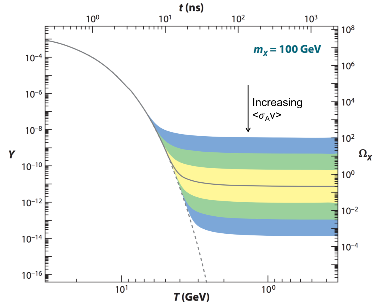
Figure 1.10: Comoving number density $Y$ of WIMPs over time $t$ with $\left\langle\sigma_{A}v\right\rangle$ that produces the correct relic density $\Omega_{\chi}$ (solid gray line). The contours of the colored bands differ from this value by 1, 2, and 3 orders of magnitude. The dashed gray line shows the number density of WIMPs that remains in thermal equilibrium. Figure modified from [33].

The relic density of WIMPs today can be obtained from the Boltzmann equation:

$$\Omega_{\chi}h^{2}\simeq\frac{T^{3}}{M_{Pl}^{3}\left\langle\sigma_{A}v\right\rangle}$$ (1.11)

where $h$ is the dimensionless Hubble parameter, $h=H_{0}/\left(100\,\mathrm{km\cdot s^{-1}\cdot Mpc^{-1}}\right)$, $T$ is the current temperature of the CMB, $M_{Pl}$ is the Planck mass, $c$ is the speed of light, $\sigma_{A}$ is the total annihilation cross section of a pair of WIMPs into SM particles and $v$ is the relative velocity between two WIMPs [21, 50]. A solution to Equation 1.11 yields

$$\Omega_{\chi}h^{2} \approx\frac{3\times 10^{-27}\,\mathrm{cm^{3}\cdot s^{-1}}}{\left\langle\sigma_{A}v\right\rangle}$$ (1.12)

$$\approx\frac{0.1\,\mathrm{pb\cdot c}}{\left\langle\sigma_{A}v\right\rangle}.$$ (1.13)

This result is roughly independent of the WIMP mass and results in fewer relic particles after freeze-out for a higher annihilation rate as illustrated in Figure 1.10 for a $100\,\mathrm{GeV/c^{2}}$. For a particle with electroweak scale interactions, the relic abundance in Equation 1.12 naturally generates WIMPs with a relic density consistent with that required for DM, $\Omega_{c}$. This is sometimes referred to as the “WIMP miracle.”

The currently best-motivated WIMP candidates are superparticles in the minimal supersymmetric model (MSSM), which is the simplest supersymmetry (SUSY) extension to the SM. SUSY was proposed to unify the electroweak, strong and gravitational forces, and it matches each particle of the SM to its partner with a different spin. Some of the candidates for WIMP from the MSSM are the gravitino, sneutrino, or neutralino (a mix of gaugino and higgsino [51]). These are stable, electrically neutral, and are expected to be massive enough to contribute to the DM abundance substantially. For more information about WIMPs consult for example [52, 53, 54, 55].

1.3 Detection strategies

Given the existence of DM, the experimentalist asks how it can be detected. The detection techniques can be broadly classified into three main categories as outlined in Figure 1.11: production, indirect detection, and direct detection. The discussion of those three techniques follows, with a focus on direct detection strategies. The primary goal of these detectors is to probe the properties of the DM particles, like their interaction mechanism or scattering rate.

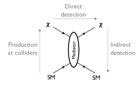
Figure 1.11: Schematics of the various detection methods. The DM particle is denoted by $\chi$.

1.3.1 Production

Production of DM can be achieved using accelerators such as the Large Hadron Collider (LHC) at the European Organization for Nuclear Research, better known as CERN. The pair production shown in Figure 1.11 does not leave any observable signal in the detectors. Instead, experiments like ATLAS and CMS search for higher order interactions: $p\bar{p}\rightarrow\chi\bar{\chi}+\mathrm{jets}$, $\gamma$s, or other particles that can serve as a trigger signaling an event. Reconstruction of event energies enables inference of missing energy and momentum after a collision. This could potentially signal a DM particle leaving the detector. However, the interpretation of these results requires an assumption of a DM model on the nature of the mediator and the corresponding operator. Excess beyond the SM has yet to be observed [56, 57].

1.3.2 Indirect

Indirect detection methods look for DM annihilation products where DM density is expected to be high, such as at the center of the Sun, in the center of our galactic halo, or in the center of nearby galaxies. DM annihilation can produce a number of particles; indirect searches look for gamma rays, neutrinos, and positron annihilation remnants. Most of these searches are subject to many backgrounds resulting from physical processes that are poorly understood, which means that it is challenging to obtain reliable background simulations [58]. An advantage of indirect searches is their ability to probe the WIMP annihilation cross section $\left\langle\sigma_{A}v\right\rangle$ directly. If a single particle constitutes DM, the value has been calculated to be $\left\langle\sigma_{A}v\right\rangle\simeq 2.2\times 10^{-26}\,\mathrm{cm^{3}/s}$ for DM masses above $10\,\mathrm{GeV/c^{2}}$ [59], often referred to as the thermal relic cross section.

There are multiple different types of indirect DM searches; consult, for example [60, 61] for an in-depth review. Satellites, such as Fermi-LAT, can be used to search for a monoenergetic line in the $\gamma$ spectrum usually from dwarf galaxies as those have relatively little astrophysical backgrounds [62]. Interactions of $\gamma$-rays in the atmosphere create a cascade of secondary particles that produce Čerenkov radiation detectable in ground-based imaging Air Čerenkov telescopes. There are numerical backgrounds present in these searches that require extensive simulations [63].

DM annihilation can also create high energy neutrinos. Those can be detected by the IceCube [64, 65], ANTARES [66], or Super-Kamiokande [67]experiments, that look for Čerenkov light generated in ice or water. Unlike the terrestrial $\gamma$-ray excess searches, detection of muon tracks would be a strong indication of DM due to a lack of other production processes. DM could scatter in the Sun causing them to lose enough energy to be captured gravitationally. As they sink to the core, they can annihilate and produce an excess of neutrinos [68]. These neutrino detectors have placed strong limits on spin-dependent (SD) scattering cross section, but unlike direct detection limits, their results are strongly dependent on assumptions for the DM annihilation process and are, therefore, strongly model-dependent.

Finally, detection of a positron excess can be a complementary probe of DM. Despite several experiments observing a positron excess [69, 70, 71], it is more likely that nearby pulsars provide the dominant contribution of this signal [72].

1.3.3 Direct

Direct detection searches look for the interaction of the Milky Way DM halo with nuclei in detectors. Assuming that WIMPs interact via the weak force, their scattering will cause a recoil of the atomic nucleus in the target medium. This recoil produces three signals in the detectors: ionization, scintillation, and heat or phonons. Most DM detectors then look for one of, or a combination of, those three signals, which enables the measurement of the event rate as a function of recoil energy. In comparison, most backgrounds caused energy depositions of radioactive decays or other charged particles result in an electron recoil in the target medium, a feature used for background discrimination. Here we focus our attention on the interaction of WIMPs, but that is indeed not the only type of DM that researchers are trying to detect directly. Even the detectors built primarily to search for WIMPs conduct many different analyses for other types of DM. Additionally, different detectors are optimized to search for other particles, such as dedicated axion searches [73, 74].

1.3.3.1 WIMP event rates in detectors

The energy transfer during a non-relativistic elastic WIMP-nucleus interaction, illustrated in Figure 1.12, is given by

$$E_{R}=2\frac{\mu_{N}}{m_{\chi}}v^{2}\cos^{2}\left(\theta\right)$$ (1.14)

where $m_{\chi}$ is the WIMP mass, $\mu_{N}=m_{\chi}m_{N}/\left(m_{\chi}+m_{N}\right)$ is the WIMP-nucleus reduced mass, $\theta$ is the initial direction of the WIMP, and $v$ is the velocity of WIMP in the lab frame [75].

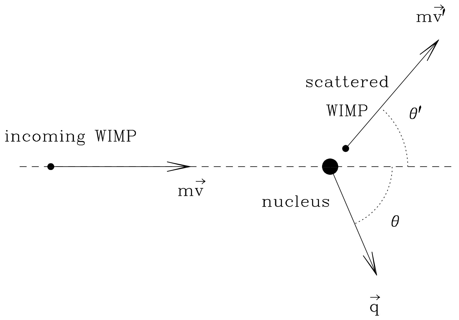
Figure 1.12: Kinematics of elastic WIMP-nucleus scattering. Figure from [76].

The quantity of interest is the number of events caused by WIMPs at a given recoil energy, so we wish to calculate the rate of WIMP-nucleus scattering as a function of energy $dR/dE_{R}$ in the detector. This differential rate (the number of events per unit time per unit energy) is the product of the number of nuclei in the detector, the WIMP flux, and the WIMP-nucleus cross section. The rate depends on the coupling strength of a WIMP to SM, while the size of the energy deposition depends on the kinematics of the DM-nucleus interaction. Below we focus on the physics aspects of this calculation. A thorough derivation of the WIMP-nucleus cross section can be found, for example, in [77, 52]. Additionally, Chapter 4 presents an overview of scattering rates for sub-GeV DM interactions caused by Bremsstrahlung and the Migdal effect expected in the LUX detector.

WIMP velocity

To find the WIMP flux, consider that the Earth is moving around the galaxy through a DM halo with local density $\rho_{\chi}$, composed of WIMPs with mass $m_{\chi}$. To calculate the WIMP flux through the Earth, we assume a DM halo with an isotropic Maxwellian velocity distribution $f(\mathbf{v})$. The distribution is truncated at the Milky Way galaxy’s escape velocity $v_{esc}$ since WIMPs traveling faster than this speed will not be gravitationally bound to the galaxy. The dominant component of the Earth’s velocity is the motion of the Sun around the Galactic center. The resulting velocity distribution has been calculated in [79, 80], and can also be seen in Equation 4.11. Additionally, the Earth’s velocity varies periodically due to its rotation about the Sun. This effect is expected to produce an annual modulation in the WIMP flux, peaked around June.

A minimum WIMP velocity

$$v_{min}=\sqrt{\frac{E_{R}m_{\chi}}{2\mu_{N}^{2}}}$$ (1.15)

is needed for a scattering event to occur; lighter WIMPs require higher velocities in order to be detected. From a kinematic standpoint, the best-suited target material is the one whose nucleus mass is closest to the WIMP mass. This is one reason why xenon detectors have an advantage in heavy WIMP detection, while detectors with lighter target materials like He, O, Si take the lead when it comes to probing lighter DM [81].

WIMP-nucleus cross section

Next, consider the WIMP-nucleus cross section $\sigma$. It is conventionally expressed as the product of $\sigma_{0}$ at the coherent scattering limit in which the WIMP interacts with the entire nucleus assuming $q=0$ momentum transfer and a nuclear form factor $F^{2}\left(q\right)$. The form factor accounts for the loss of coherence in the scattering amplitudes per nucleon due to $q>0$, and generally has an exponential form. It becomes relevant when the wavelength $h/q$ of the momentum transfer is on the same scale as the effective nuclear radius $r_{n}$. For example, for xenon $r_{n}\simeq 6\,\mathrm{fm}$, which corresponds to recoil energy of 5 keV. For spin-independent (SI) interactions, the form factor is given by the Fourier transform of the density of nucleon distribution in the nucleus. A widely-used nuclear form factor for DM calculations is the Helm form factor [82], also known as the Woods-Saxon potential. For further discussion of SI form factors, refer to Sections 4.1.1, 4.1.2, and 4.2.1. Calculations of form factors for SD scattering are more intriguing since they require a knowledge of the quark contents of the nucleus and are discussed in [84, 85].

WIMPs can either couple to the mass of the nucleus, referred to as SI scattering, mediated by a scalar, or to the spin of the target nucleus, referred to as SD scattering, mediated by an axial-vector. The SI interaction cross section is given by [90]:

$$\sigma_{SI}=\frac{4}{\pi}\mu_{N}\left[Zf_{p}+\left(A-Z\right)f_{n}\right]^{2}$$ (1.16)

where $Z$ is the atomic number and $A$ is the atomic mass of the target nucleus (so $A-Z$ is the number of neutrons), and $f_{p}$ and $f_{n}$ are the effective scalar couplings of WIMPs to protons and neutrons, respectively. Since $f_{n}\simeq f_{p}$ in most theoretical models, the SI cross section can be simplified to

$$\sigma_{SI}\simeq\frac{4}{\pi}\mu_{N}^{2}A^{2}\left|f_{p}\right|^{2}.$$ (1.17)

This can be rewritten as

$$\sigma_{SI}\simeq\sigma_{n}\frac{\mu_{N}^{2}}{\mu_{n}^{2}}A^{2}$$ (1.18)

to factor out the effect of the target material. Here $\mu_{n}$ is the WIMP-nucleon reduced mass, and the target-independent spin-independent cross section of a WIMP on a single nucleon is given by

$$\sigma_{0}^{SI}=\frac{4}{\pi}\mu_{n}^{2}f_{p}^{2}.$$ (1.19)

The SD cross section is

$$\sigma_{SD}=\frac{32}{\pi}G_{F}^{2}\mu_{N}^{2}\frac{J+1}{J}\left[\left\langle S_{p}\right\rangle a_{p}+\left\langle S_{n}\right\rangle a_{n}\right]^{2}$$ (1.20)

where $G_{F}$ is the Fermi constant, $J$ is the total spin of the target nucleus, and $\left\langle S_{p,n}\right\rangle$ and $a_{p,n}$ refer to the expectation values of the proton and neutron group spins and SD couplings, respectively. Notice that the SI scattering benefits from higher-mass nuclei, while the SD scattering is related to target nuclei with an unpaired nucleon.

Combining the above yields the standard WIMP scattering event rate [90]

$$\frac{dR}{dE_{R}}=\frac{\rho_{\chi}}{2m_{\chi}\mu_{N}}\sigma_{0}F^{2}\left(E_{R}\right)\intop_{v_{min}}^{v_{esc}}\frac{f(\mathbf{v})}{v}d^{3}v.$$ (1.21)

As discussed above, the DM distribution is included in $\rho_{\chi}$ and the velocity integral, while the nuclear and particle physics aspects are included within $\sigma_{0}F^{2}\left(E_{R}\right)$. Integrating Equation 1.21 yields the number of expected events in a detector for a given choice of target, as illustrated in Figure 1.13. The low event rates mean that in order to see DM, detectors need to focus on background reduction. The exponential tail caused by the form factor results in detector technologies pushing detection threshold to low energies. Additionally, present-day experiments use various targets since each will be most sensitive to a different WIMP mass.

Even though DM has not yet been detected directly, the non-detection results, presented as limits on WIMP-nucleon interactions (see, for examples Figures 2.32, 4.15, or 4.16), are helpful since they constrain the theoretical DM models.

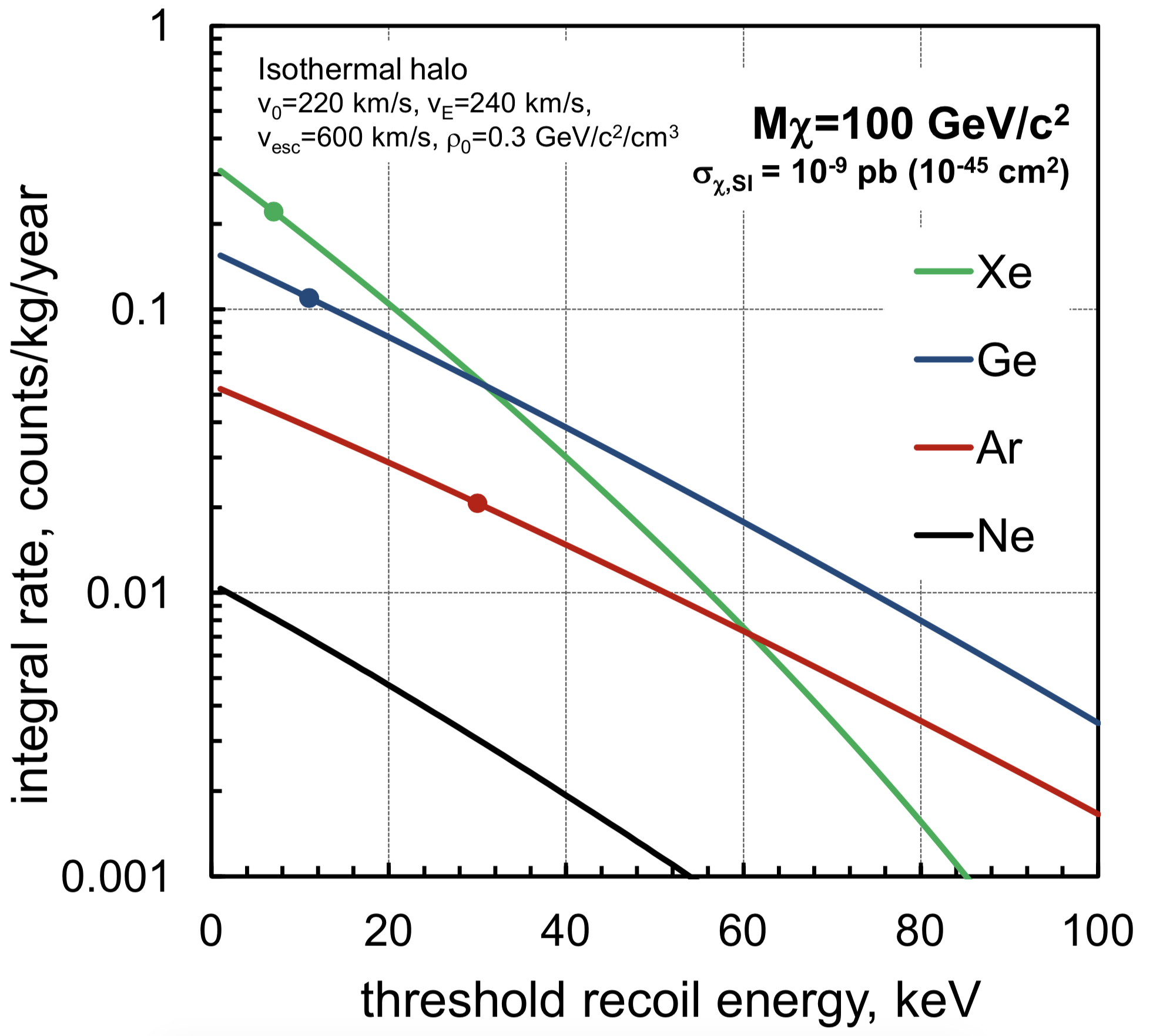
Figure 1.13: Predicted integral spectra for WIMP-nucleus elastic scattering assuming perfect detector energy resolution for various materials: Xe ($A=131$), Ge ($A=73$), Ar ($A=40$), and Ne ($A=20$). The spectra are calculated for a $100\,\mathrm{GeV/c^{2}}$ WIMP with $\sigma=10^{-45}\,\mathrm{cm^{2}}$ interaction cross section per nucleon and the halo parameters shown in the figure. The circles on each curve indicate the typical WIMP search threshold for each material. Figure from [91].

1.4 Direct dark matter detection technologies

Given the WIMP interaction rates outlined in the previous section, various technologies can be leveraged to search directly for these particles here on Earth. Detectors primarily focus on interactions of WIMPs with nuclei by elastic scattering, which requires detecting nuclear recoil energies in the $1-100\,\mathrm{keV}$ range [77] while being sensitive to cross sections of order $10^{-35}-10^{-48}$ cm². These very low energies and cross sections constitute an experimental challenge, but the field has achieved steady progress since the 1990’s as shown in Figure 1.14: sensitivity of detectors looking for SI WIMP-nucleus interactions has been doubling every 18 months.

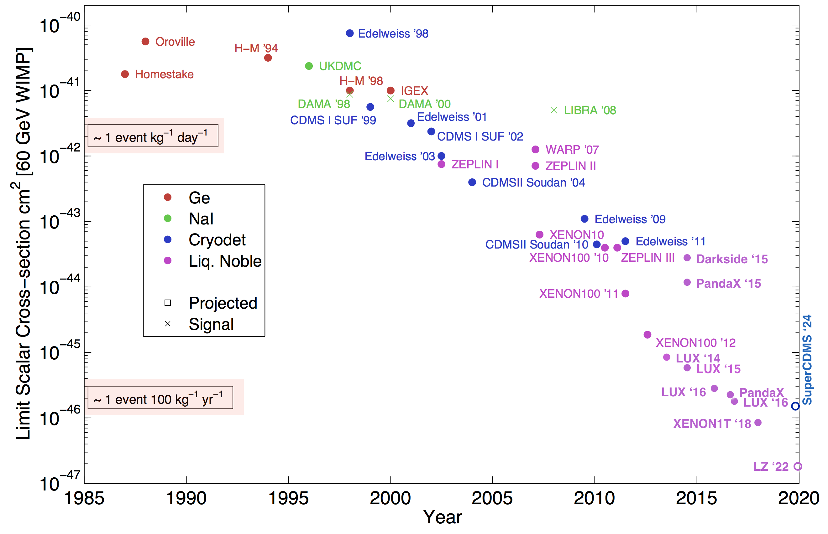
Figure 1.14: Evolution of the WIMP-nucleon spin-independent cross section limit for a WIMP mass of $60\,\mathrm{GeV/c^{2}}$. Different colors correspond to various detector technologies. Empty markers indicate predicted performance. Liquid noble detectors have been the leading technology for direct dark matter detection. Figure from [92].

A variety of materials are used in detector construction to leverage their diverse benefits: lighter detectors using Si or Ge lead the way in the search for lighter WIMPs, while for WIMP masses $\apprge 5\,\mathrm{GeV/c^{2}}$ the most stringent limits are set by xenon detectors. Broad complementarity of searches is important both to probe a spectrum of DM candidates, but in case of detection, independent confirmations from various independent sources will be necessary. This section briefly discusses some of the detector methods currently used for direct DM detection, with a focus on technologies that have reached the best limits to date; Figure 1.15 shows a graphical overview of the detector technologies discussed. For more information on direct detection experiments, see for example [93, 94, 95, 96].

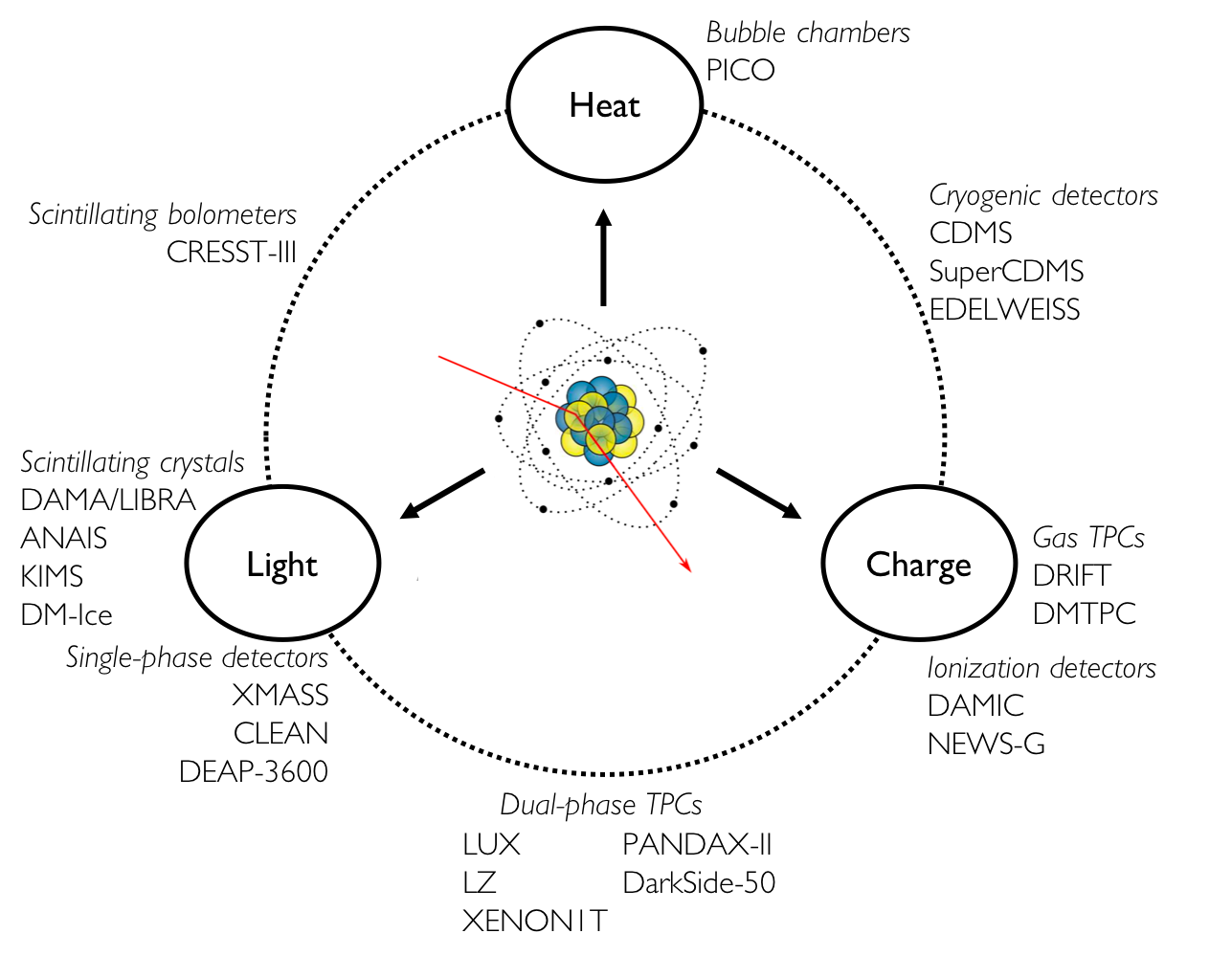
Figure 1.15: Possible signals in direct detection and a sample of experiments leveraging various channels.

Despite various technologies used in the detectors discussed, for the majority of detectors background reduction is of utmost importance; detectors use passive shielding, low radioactivity materials, and environment, which frequently results in their underground location. Limits obtained by many of the collaborations described below are also included in Figure 4.15 in Chapter 4 that focuses on sub-GeV DM searches with the LUX detector.

1.4.1 Noble gas detectors

Noble liquid detectors are the current leaders in sensitivity to WIMP masses $\lesssim 5\,\mathrm{GeV}$. Four noble gasses have been considered for DM detection: helium [97], neon [98], argon, and xenon. Only argon and xenon detectors have thus far placed limits on DM interactions. The most successful xenon detectors are two-phase time projection chambers (TPC), of which LUX is one example, described in great detail in Chapter 2. This approach was pioneered by the ZEPLIN [99] and XENON10 experiments [100]. The LUX detector was the first to achieve sub-zeptobarn ($<1\times 10^{-45}\,\mathrm{cm^{2}}$) sensitivity [101]. Currently, there is a tight race between three collaborations building detectors with increasing target mass: PandaX [102] located at the JinPing underground laboratory (CJPL) in China, XENON1T [103] and its planned upgrade XENONnT located in the Gran Sasso National Laboratory (LNGS) in Italy, and LZ [104], discussed in Chapter 5, planned to start operations in 2019 at the Sanford Underground Research Facility in the USA. Looking ahead, the DARWIN (DARk matter WImp search with liquid xenoN) collaboration is considering a detector with up to 40 tons of target mass [105].

An alternative to the two-phase TPC is the single phase detector. Since single-phase detectors only use scintillation signal, position reconstruction of interaction vertices is a significant challenge. One such xenon detector is currently operational, the XMASS (Xenon detector for Weakly Interacting MASSive Particles) experiment at the Kamioka Observatory in Japan. Its PMTs cover more than 62% of the inner surface in $4\pi$ resulting in large photoelectron yield [106, 107].

Argon is frequently used as an alternative to xenon due to its lower cost, which allows construction of more massive detectors leading to more exposure. However, the presence of the radioactive isotope of ³⁹Ar hinders the performance of these detectors in DM searches; this limitation can be partially overcome by using underground argon [108, 109, 110] or through distillation [111] to reduce the ³⁹Ar content. There are currently three detectors using LAr for DM detection: the DarkSide collaboration uses a two-phase TPC technology [112], while DEAP-3600 (Dark Matter Experiment using Argon Pulse-shape) [113] and MiniCLEAN (Cryogenic Low-Energy Astrophysics with Noble liquids) [114] utilize the single-phase technology. Unlike in xenon, the argon scintillation long-lived triplet and the short-lived singlet states have very different decay times. This enables pulse shape discrimination which can achieve background reduction by $10^{-7}$ [112]. This means that good background rejection can be achieved using only the scintillation signal. A thorough review of technological advances for both light and charge can be found in [91].

1.4.2 Cryogenic solid state detectors

Cryogenic detectors operate below 100 mK and aim to detect small increases in temperature. They provide the leading limits for WIMP masses $\lesssim 5\,\mathrm{GeV/c^{2}}$ by detecting phonons produced within the crystal lattice by scattering of individual DM particles. The CDMS (Cryogenic Dark Matter Search) collaboration was the first to deploy such a detector using germanium and silicon crystals initially at a shallow site at the Stanford Underground Facility [115] and then at the Soudan Underground Laboratory in Minnesota, USA [116]. The detectors are sensitive to both the phonon (heat) and ionization signals and provide excellent discrimination of electron recoils via ionization/heat ratio and pulse shape discrimination (with a misidentification rate of less than 1 in $10^{6}$). The phonons are detected using transition edge sensors while an electric field is set up to collect the ionization charge. The SuperCDMS collaboration uses advanced technology with improved identification of background events near the surfaces of the crystals [118, 119]. SuperCDMS is planning an increase in detector mass and exposure, as well as relocation to a deeper lab (SNOLAB in Sudbury, Canada) in order to reduce backgrounds and search for WIMP masses between 0.5 and $7\,\mathrm{GeV/c^{2}}$ [120].

The leading limits for low mass WIMPs below $1.8\,\mathrm{GeV/c^{2}}$ were obtained by the CRESST (Cryogenic Rare Event Search with Superconducting Thermometers) collaboration. The CRESST-II experiment used 300 g of CaWO₄ crystals operating at $\sim 10\,\mathrm{mK}$ located at LNGS. By detecting phonons and scintillation signal with an energy threshold of $\sim 300\,\mathrm{eV}$, they were the first to place nuclear recoil cross section limits on DM with masses below $1\,\mathrm{GeV/c^{2}}$ [121]. The upgraded detector with smaller crystals and an improved threshold of $<100\,\mathrm{eV}$, CRESST-III has released preliminary improved limits compared to its predecessor [122]. The collaboration recently placed limits on DM masses down to $140\,\mathrm{MeV/c^{2}}$ using a prototype 0.5 g sapphire (Al₂O₃) detector operating on the surface [123, 124]. The EDELWEISS collaboration is also using cryogenic germanium detectors for phonons and ionization signals for DM searches [125, 126].

1.4.3 Superheated liquid detectors

Bubble chambers and superheated droplet detectors provide the leading limits for SD WIMP-proton interactions. Only energy depositions from nuclear recoils or $\alpha$ events with large enough energy will create a bubble in a superheater liquid detector, which can then be photographed and acoustically recorded. The use of acoustics allows discrimination of $\alpha$ background events that also have enough energy for bubble nucleation. Since ER will not deposit enough energy to trigger a formation of bubbles, this technique features strong ER background discrimination. However, this technique requires one to perform a scan over various operating temperatures and pressures to produce an energy spectrum, rather than measuring energy on a per-event basis. The PICO collaboration is currently operating two chambers and has tested two different liquids C₃F₈ and CF₃I in SNOLAB [128, 129].

A recent R&D effort at Northwestern University used a 30 g xenon bubble chamber to detect nuclear recoils using both simultaneous scintillation and bubble nucleation. This chamber is instrumented with a PMT, and a near-IR camera and a piezoelectric acoustic transducer to detect bubbles. The detector combines an improved electron recoil rejection compared to CF₃I with an energy resolution of a liquid scintillator. The improved electron recoil rejection is likely caused by the scintillation production suppressing bubble nucleation by electron recoils, while nuclear recoils remain unaffected [130]. This approach may allow both energy reconstruction (by measuring scintillation) and ER background rejection (by detecting bubble formation).

1.4.4 Scintillating crystals

The most notable example of the use of scintillating crystals is the DAMA/LIBRA experiment that observed an annual modulation in the event rate in 250 kg of scintillating inorganic NaI(Tl) crystals that they attribute to a DM signal [131, 132]. This experiment is a successor to the DAMA/NaI experiment which observed an annual modulation throughout 1995-2002 with $\sim 100\,\mathrm{kg}$ of NaI(Tl) crystals [133]. Their claim is not compatible with the WIMP hypothesis and has been refuted by many other experiments’ null results using other detector materials. The majority of the DM community is skeptical of the DAMA/LIBRA results, see for example [134, 135, 136, 137].

Nevertheless, efforts to test their results using NaI detectors are underway. The SABRE (Sodium Iodide with Active Background REjection) collaboration plans to operate one detector each on the northern (at LNGS) and southern hemispheres (at the Stawell gold mine in Victoria, Australia). This will reduce the chance for false positives from possible seasonal systematic effects [138]. The COSINE-100 experiment is a joint effort between the DM-Ice [139] and KIMS [140] collaborations located at the Yangyang Underground Laboratory in Korea. Its first 106 kg of low-background NaI(Tl) has been taking physics data since September 2016 [141]. Lastly, ANAIS–112 (Annual modulation with NaI Scintillators) is a dark matter search using 112.5 kg of NaI(Tl) scintillators located at the Canfranc Underground Laboratory in Spain [142, 143].

1.4.5 CCD chips

The DAMIC (DArk Matter In CCDs) experiment uses high resistivity charge-coupled silicon detectors (known as CCD chips) to record ionization signals produced in the silicon pixels [144]. They have recently released a result using 23.2 g of material with 0.6 kg-day exposure at SNOLAB for WIMP masses below $10\,\mathrm{GeV/c^{2}}$ [145]. A larger detector, DAMIC100 with 100 g of material is being deployed at the same place, and a 1-kg detector DAMIC-M has been approved for installation at the Laboratoire Souterrain de Modane (LSM) in France.

1.4.6 Spherical proportional counters

The NEWS-G (New Experiments With Spheres-Gas) is a large copper vessel filled with a mixture of Ne and CH₄ with a small high voltage sensor in its center. This creates a graded electric field in the detector that causes an avalanche process if an ionization electron is generated. Therefore, the detector features a very low energy detection threshold. The detector is located at LSM and recently published new limits [146].

1.4.7 Directional detection

Directional detectors are trying to detect the “WIMP wind” from the motion of Earth through the galaxy using low-pressure gas TPCs. The low-pressure gas allows 3D reconstruction of particle tracks; particles that pass through the detector in directions other than the expected WIMP wind are deemed background. Additional background discrimination comes from track length. One of the main drawbacks of these detectors is their low-pressure nature since a large ($1\,\mathrm{m^{3}}$) detector contains only $\sim 100\,\mathrm{g}$ of target mass making it difficult to reach large exposures. This type of detectors was pioneered by the DRIFT (Directional Recoil Information From Tracks) collaboration. Rather than drifting ionization charge, the detector drifts negative ions that captured liberated electrons in particle interactions. The DRIFT detector was installed in the Boulby mine in the UK and was filled with either CS₂ or CF₄ gas mixtures and currently has achieved the leading limit among the directional detectors for SD WIMP-nucleon scattering for WIMP masses above $10\,\mathrm{GeV}/c^{2}$ [147]. A detector upgrade with a larger active volume is underway [148]. The DMTPC m³ experiment [149] uses light and charge readout to measure the directional anisotropy of nuclear recoils. Most collaborations working on directional detection are planning to join their forces in the CYGNUS collaboration [150].

1.4.8 Overview of the status of the field

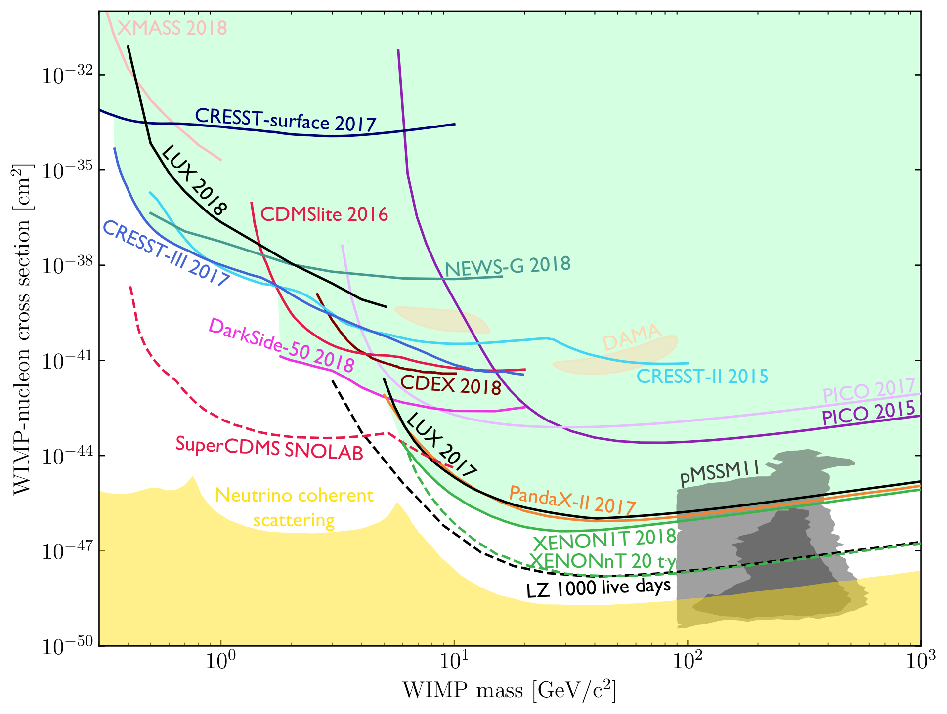
Figure 1.16: A compilation of WIMP-nucleon spin-independent cross section limits (solid curves), DM signal hints (closed contours), and projections (dashed curves). Limits for a heavy mediator along with limits from the spin-independent analyses of LUX [127, 151] (black), PandaX-II [102] (orange), XENON1T [103] (green), CDEX-10 [152] (maroon), CDMSlite [119] (red), CRESST-II [121] (cyan), CRESST-III [122] (blue), CRESST-surface [123] (navy), DarkSide-50 [153] (magenta), NEWS-G [146] (teal), PICO C₃F₈ 2017 [154] (purple), PICO CF₃I 2015 [129] (lavender), and XMASS [107] (pink). The dashed curves show projections for LZ [104] (black), XENONnT [155] (green), and SuperCDMS SNOLAB [156] (red). Also shown is a hint for a WIMP signal from DAMA [157] (orange). The yellow region indicates a background from coherent neutrino-nucleus scattering [158]. The gray region shows predictions from pMSSM11 [159, 160].

Figure 1.16 shows a compilation of limits and signal hints for WIMP-nucleon spin-independent interactions from some of the experiments discussed above, as well as projections from future experiments. As detectors become more sensitive, they approach an irreducible background from coherent neutrino-nucleus scattering, which limits their discovery potential. The so-called “neutrino floor” is shown for a xenon target with no other backgrounds, 100% efficiency, an energy threshold of 3 eV, and a 1000 ton-year exposure as calculated in [158]. Also shown is the prediction region from the phenomenological MSSM (pMSSM11) constrained using the MasterCode [159, 160]. The MasterCode compiles current experimental data and allows fits to different versions of MSSM.

The non-detection of WIMPs with masses larger than a few GeV/c² has led to an increase of detection efforts in the sub-GeV region. This includes both a focus on the development of new detector technologies (e.g., [97]) and a focus of current experiments on increasing their sensitivity to lower mass DM as discussed in Chapter 4.

1.5 Summary and outline

The existence of DM is well motivated, with many potential candidate particles and detection mechanisms. The rest of this manuscript dives into the various aspects of direct detection of DM using a two-phase xenon time projection chamber. The detector technologies are quickly maturing, thanks to a large number of R&D efforts. This enables scaling of the detectors to achieve unprecedented low background, which might lead to convincing evidence for positive DM signal in the future.

Chapter 2 provides an overview of the LUX detector, which led the field for several years. The remainder of this dissertation then discusses original work related to direct DM detection. Chapters 3 and 4 are devoted to original work pertaining to LUX: Chapter 3 discusses 3D modeling of electric fields of the LUX detector and Chapter 4 presents limits on sub-GeV DM using the 2013 LUX dataset. Chapter 5 starts with an overview of the LZ detector, the successor to LUX, and then discusses design and construction of a couple of noble liquid purity monitors used in high voltage research and development (R&D). Finally, Chapter 6 describes the design, construction, and data acquisition of the Xenon Breakdown Apparatus (XeBrA), designed to study the breakdown behavior of noble liquids. Additionally, since a diverse body of researchers is essential for success, Appendix A presents a synopsis of the Equity & Inclusion work done as part of the LZ collaboration.

Chapter 2 The LUX experiment

The Large Underground Xenon (LUX) experiment was a two-phase liquid-gas xenon time projection chamber (TPC) containing 370 kg of xenon. LUX was formed by $\sim 100$ collaborators from 24 institutions in the USA, UK, and Portugal. This chapter covers the basics of two-phase TPC operations, the design of the LUX detector, highlights of some its subsystems and calibration techniques, and provides an overview of the data analyses leading to several world-leading exclusion limits for WIMP-nucleon elastic scattering.

2.1 Two-phase time projection chambers

Originally, single-phase gas filled projection chambers were developed for high-energy physics in 1974 by David R. Nygren at Lawrence Berkeley National Laboratory (LBNL) [161]. The design was modified and applied to a single-phase liquid argon TPC in 1977 by Carlo Rubbia [162]. Over time, thanks to their particle detection capabilities, both single and two-phase noble gas TPCs have been deployed throughout the experimental direct dark matter field using xenon [163, 164, 102] and argon [108, 114, 165, 166]. However, the development and refinement of two-phase TPCs unlocked an opportunity for improved detection and exclusion mechanisms. Nowadays, two-phase xenon TPCs provide the most stringent limits on WIMP candidates with masses of $\sim 5$-100,000 GeV/c² due to their low intrinsic backgrounds, position reconstruction and discrimination between electron and nuclear recoils, which enables excellent background rejection.

In a two-phase TPC, scintillation and ionization signals produced by excitations of xenon atoms and electron-ion pairs can be detected. This provides a crucial feature of TPCs as dark matter detectors since this light-to-charge ratio is far lower for recoiling nuclei, caused either (ideally) by WIMPs or by neutron scattering, than for recoiling electrons, which are caused by the vast majority of background interactions. Figure 2.1 illustrates the operation of the LUX detector. First, a particle traveling through a detector collides with a xenon atom and deposits energy in the form of prompt scintillation (light), ionization (charge), and heat. The scintillation light is detected within 100 ns using sensitive light detectors known as photomultiplier tubes (PMTs) at the top and bottom of the detector volume. This primary signal is referred to as S1. The ionization electrons liberated during the collision drift to the top of the detector in the presence of an electric field. The electrons are extracted out of the liquid xenon using a stronger electric field established by a pair of grids. This accelerating cloud of electrons creates a secondary proportional scintillation signal (S2), also known as electroluminescence, as it travels through a thin layer of gaseous xenon.

The TPC provides a wealth of information for each scattering event: its energy, the event location within the detector, and whether it is an electron or nuclear recoil. The total energy deposited in the event can be estimated from a linear combination of the sizes of the S1 and S2 signals. The location of the event can be reconstructed from the S1 and S2 signals: the $\left(x,y\right)$ position of the event is given by the distribution of S2 photons incident on the top PMT array with up to millimeter resolution and the $z$ coordinate is given by the time separation of the S1 and S2 signals, given by the electron drift time. Furthermore, the ratio of the S2 and S1 signals differs for electron recoils (ER) and nuclear recoils (NR). In ERs, an incident particle scatters off a bound electron, or a $\beta$ decay occurs. The majority of ERs are generated from background events, mostly stemming from radioactivity such as $\beta$, x-rays, and $\gamma$ radiation. It is expected that WIMPs would cause NRs, along with interactions from background neutrons. Distinguishing NRs from ERs is, therefore, a crucial tool for improving dark matter searches.

As might be clear, many pieces need to come together to enable dark matter searches. First, a dark matter search entails building the detector (Section 2.2.1) and thoroughly understanding its operations and operating conditions (Sections 2.2.2 and 2.2.3). This starts by interpreting interactions occurring inside the detector by understanding xenon microphysics (Section 2.1.1), describing efficiencies of detection of light and charge generated by the interaction (Section 2.2.6), performing signal processing (Section 2.2.4), interpreting the data correctly and conducting appropriate analysis (Section 2.2.5) before generating the final result. The construction and signal interpretation is the bulk of the work in detector science, but appropriate software modeling, accurate simulation of the detector itself, backgrounds present and particle interactions are also important (Section 2.3). Information for the background simulation is obtained via a thorough radioactive screening campaign of the detector materials and parts. This information can be implemented in the detector’s 3D simulation software, and with a simulation of xenon physics, all the models needed for the final result can be built. Together all those efforts contribute to the great science done by the LUX experiment over the years (Section 2.4).

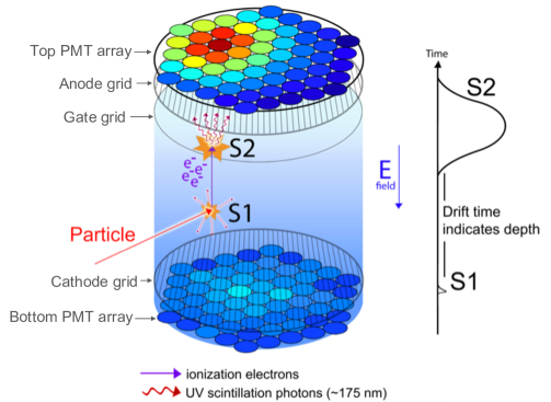
Figure 2.1: Illustration of detection principles of a two-phase TPC. A particle interacts with a xenon atom and produces prompt scintillation photons (S1) that get detected by the PMT arrays and ionization electrons. The electron cloud drifts against the applied electric field to the top of the detector, where it creates a secondary proportional scintillation signal (S2) in the gas. The S2 signal is detected by the top PMT array and enables $\left(x,y\right)$ position reconstruction on the order of millimeters. The depth of the event is given by the time separation between the S1 and S2 signals. The amount of liquid xenon enclosed between the gate and cathode grids and the detector walls is called the active volume. Figure by Carlos Faham.

2.1.1 Liquid xenon physics

Liquid xenon (LXe) provides several advantages for dark matter detection. This section first gives a synopsis of xenon qualities that make it a suitable element for dark matter searches and then provides a characterization of xenon’s response to particle interaction and energy deposition reconstruction techniques.

Xenon is the heaviest of the stable noble gases with atomic number $Z=54$ and atomic mass $A=131.293(6)\,\mathrm{g}$. Xenon’s high density of $\sim 2.95$ g/cm³ at $170\,\mathrm{K}$ enables compact detector design and allows for efficient self-shielding, creating an ultra-low background inner detector volume (also referred to as “fiducial volume”) suitable for rare event searches. The most significant impact of self-shielding against typical external gamma-rays is realized in the outermost few centimeters of xenon, as illustrated in Figure 2.2, and $\beta$-rays penetrate even shorter distances. The high mass number $A$ also results in good sensitivity to the spin-independent (SI) WIMP-nucleon interaction, and a 48% abundance of neutron-odd isotopes enables sensitivity to the spin-dependent (SD) WIMP-neutron interaction; the list of all known natural xenon isotopes is in Table 2.1. Xenon has essentially no long-lived naturally abundant radioactive isotopes, except for the $2\nu\beta\beta$ decay of ¹³⁶Xe with a measured half-life of $2.2\times 10^{21}$ years [168, 169]. Xenon also has only moderate cryogenic requirements with a triple point of $161\,\mathrm{K}$, and commercial gas-phase xenon purifiers (getters) are available for the removal of electronegative and light-absorbing impurities such as O₂ and N₂. Furthermore, xenon is transparent to its scintillation light with wavelength $\lambda=178\,\mathrm{nm}$ (7 eV), since this energy is lower than the first ionization potential of xenon, which is 12.1 eV.

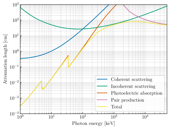
Figure 2.2: Photon attenuation length in xenon assuming $\rho_{Xe}=2.95\,\mathrm{g/cm^{3}}$. Total is the maximum attenuation length from all effects combined; the photoelectric effect dominates at low photon energies. Data from [170].

Isotope	Atomic mass/u	Natural abundance
124Xe	123.906	0.09%
126Xe	125.904	0.09%
128Xe	127.904	1.91%
129Xe	128.905	26.40%
130Xe	129.904	4.07%
131Xe	130.905	21.23%
132Xe	131.904	26.91%
134Xe	133.905	10.44%
136Xe	135.907	8.86%

Table 2.1: Atmospheric abundance of known natural xenon isotopes. Data from [167].

As mentioned above, a particle interaction in LXe deposits energy into three channels: heat, light, and charge. This energy deposition leaves xenon atoms in both excited and ionized states. Within picoseconds, the excited Xe atoms combine with neighboring Xe atoms in their ground state to form excitons, short-lived diatomic molecules Xe${}_{2}^{*}$:

$$\mathrm{Xe^{*}+Xe\rightarrow Xe_{2}^{*}.}$$ (2.1)

Excitons can exist either in their singlet state with an electron spin quantum number $s=0$ (corresponding to the state $\frac{1}{\sqrt{2}}\left(\left|\uparrow\downarrow\right\rangle-\left|\downarrow\uparrow\right\rangle\right)$) or a triplet state with a spin quantum number $s=1$ (corresponding to 3 different states: $\frac{1}{\sqrt{2}}\left(\left|\uparrow\downarrow\right\rangle+\left|\downarrow\uparrow\right\rangle\right)$; $\left|\uparrow\uparrow\right\rangle$; $\left|\downarrow\downarrow\right\rangle$). Both states de-excite by emitting a $178\,\mathrm{nm}$ vacuum-ultraviolet (VUV) photon, with a lifetime of $24\,\mathrm{ns}$ for the singlet state and $3.1\,\mathrm{ns}$ for the triplet state [173] and a FWHM of 13 nm [174]:

$$\mathrm{Xe_{2}^{*}\rightarrow 2\,Xe\,+\,}h\nu.$$ (2.2)

The ionized Xe atoms will also recombine with nearby Xe atoms on a time scale of picoseconds. Then, in the absence of an applied electric field, the excitons form excited Xe atoms by capturing nearby free electrons:

$$\mathrm{Xe^{+}+Xe} \rightarrow\mathrm{Xe_{2}^{*}}$$ (2.3)

$$\mathrm{Xe_{2}^{+}+}e^{-} \rightarrow\mathrm{Xe^{**}+Xe}$$ (2.4)

$$\mathrm{Xe^{**}} \rightarrow\mathrm{Xe^{*}\,+\,heat.}$$ (2.5)

The excited Xe atoms release addition scintillation photons according to Equations 2.1 and 2.2. This recombination process can be suppressed by the application of an electric field, which leads to a quenching of the primary scintillation yield.

The energy $E$ deposited by a particle is given by

$$E=fW\left(n_{i}+n_{ex}\right)$$ (2.6)

where the quenching factor $f$ accounts for a varying fraction of energy lost to atomic motion (heat) and the work function $W=13.7\pm 0.2\,\mathrm{eV}$ [175]. This is multiplied by the total number of quanta produced along the track of the recoiling particles, which is the sum of $n_{i}$ (the number of electron-ion pairs), and $n_{ex}$ (the number of excitons created), as discussed below. For ER the fraction of energy dissipated by heat is constant with energy, so $f_{ER}\equiv 1$ [176] and the energy heat loss is included in the value of $W$. For NR the recoiling nucleus will generate secondary recoils below the excitation threshold $W$. The microphysics of this process is described by the Lindhard theory [177]. The quenching factor for nuclear recoils varies with deposited energy. This means that in the LUX detector, an NR signal is smaller than an ER signal of the same energy.

The ratio of excitons to ions produced along the track of the recoiling particle

$$\alpha\equiv\frac{n_{ex}}{n_{i}}$$ (2.7)

can be approximated as roughly constant with $\alpha_{NR}\sim 1$ [175] and $\alpha_{ER}\sim 0.2$ [178]. However, following ionization a fraction $r$ of the initial electron-ion pairs recombines and forms additional excitons, enhancing the S1 signal. This recombination depends on LXe density, the applied electric field, and particle energy. At 180 V/cm the recombination peaks at $\sim 12\,\mathrm{keV}$ as measured by the LUX detector [179, 175, 180, 181, 182]. Therefore, the quantities directly measurable in the detector are the de-excitation photons $n_{\gamma}$ from all the excitons formed and the electrons that escape recombination $n_{e}$:

$$n_{\gamma} =n_{ex}+rn_{i}=\left(\alpha+r\right)n_{i}$$ (2.8)

$$n_{e} =\left(1-r\right)n_{i}.$$ (2.9)

The detected S1 and S2 signals are given by

$$S1= \,g_{1}n_{\gamma}$$ (2.10)

$$S2= \,g_{2}n_{e}$$ (2.11)

where the italicized scintillation ($S1$) and ionization ($S2$) signals are measured in units of detected photons (phd) in the TPC. These pulse sizes are corrected for geometrical effects in the detector and electron lifetime in LXe [183] in the data processing chain described in Section 2.2.5. The units of detected photons differ from the more commonly used unit of photoelectrons (phe) by a small factor representing the probability of a single photon to produce multiple phe in a PMT photocathode [184]. The detector efficiencies $g_{1}$ and $g_{2}$ are the signal gains for $S1$ and $S2$ in units of phd/quantum. For S1 photons $g_{1}$ is the product of geometrical light collection efficiency and the averaged PMT quantum efficiency, as it represents the probability of a scintillation photon to produce at least one phe on the PMT photocathode. For S2 photons, $g_{2}$ depends on the electroluminescence photon yield, the efficiency $\epsilon$ with which drifted electrons are extracted from the liquid into the gas phase, and the average pulse size of a single extracted electron (SE):

$$g_{2}=\epsilon\times SE.$$ (2.12)

In the LUX detector $g_{1}\sim 0.1$ and $g_{2}\sim 12$ as derived from calibrations.

Equations 2.8 and 2.9 show that, ignoring quenching effects, all excitons and electron-ion pairs result in either an escaping photon or an electron with perfect efficiency, i.e., $n_{\gamma}+n_{e}=n_{ex}+n_{i}$. Although the light and charge yields vary with energy due to dependence on recombination, the proportion of energy that goes into the combination of ionization and scintillation signal remains constant. Therefore, the combined energy from $S1$ and $S2$ can be used to reconstruct the true energy of an event. As such, Equation 2.6 can be rewritten as

$$E =fW\left(n_{\gamma}+n_{e}\right)$$ (2.13)

$$=fW\left(\frac{S1}{g_{1}}+\frac{S2}{g_{2}}\right).$$ (2.14)

This equation describes a response of a specific TPC with given operating conditions, unlike Equation 2.6, which describes the general response of LXe an energy deposit. However, while reconstructing events in the detector, it may not be known whether a particular event is the result of an electron or nuclear recoil. If the energy is reconstructed under the assumption of an ER with $f=1$, units of $\mathrm{keV_{ee}}$ are used where “ee” stands for “electron equivalent.” Similarly, if the energy calculation assumes an NR, units of $\mathrm{keV_{nr}}$ (often written without the subscript) are used. The following equation can be used to convert between those two units

$$\mathrm{keV_{ee}=}\left(\frac{12.6}{73}\right)\mathrm{keV_{nr}}^{1.05}.$$ (2.15)

It was obtained from a fit to data by NEST v2.0 [185].

The mean $S1$ and $S2$ response at two or more known energies can be used to calculate $g_{1}$ and $g_{2}$ by requiring that the combined energy from $S1$ and $S2$ reconstructs the true energy of a calibration source of known energy. Those values are described by a line $y=mx+b$ where $x=\left\langle S2\right\rangle/E$ and $y=\left\langle S1\right\rangle/E$ as shown in Figure 2.3. A fit to the slope $m=-g_{1}/g_{2}$ and $y$-intercept $b=g_{1}/W$ are then used to measure $g_{1}$ and $g_{2}$. Further details about this so-called “Doke plot analysis” can be found in [186, 187]. A more detailed review of the operation principles and the most essential instrumentation aspects of two-phase TPCs can be found in [91].

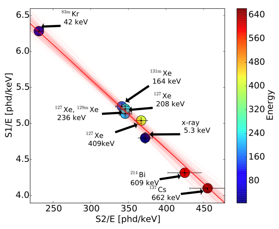
Figure 2.3: Doke plot used to calculate $g_{1}$ and $g_{2}$ in the LUX 2013 reanalysis. Each point represents a different line source collected at a drift field of 180 V/cm. Values of $g_{1}=0.117\pm 0.003$ and $g_{2}=12.1\pm 0.8$ were found. The further to the lower right a point is on the plot, the less recombination (less S1 and more S2). Figure from [186].

2.2 The LUX detector

2.2.1 Detector design

The LUX detector was a two-phase TPC located a mile underground in the Davis cavern at the Sanford Underground Research Facility (SURF) in Lead, South Dakota. The layout of the underground laboratory and the support systems needed to operate the detector is shown in Figure 2.4. As for many other rare event searches, one of the main design goals was the reduction of the rate of background events to ensure that the detector was not swamped with an unwanted signal. The underground location with $1478\,\mathrm{m}$ (4850 ft or 4300 m water equivalent) of rock overburden provides shielding from cosmogenic radiation. To that end, the detector was also located inside of a water tank, and careful material assays were performed prior to detector assembly to establish a low-background environment for the detector. Furthermore, the realities of our world such as cost, ease of operations, and safety were considered in the detector design. This section highlights selected parts of the detector; a more detailed description of the design choices for the LUX detector can be found in [190], and in-depth descriptions of the individual subsystems can be found in the various LUX theses mentioned throughout the text.

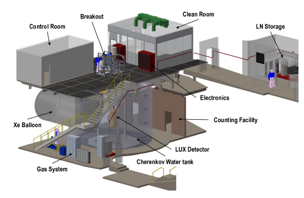
Figure 2.4: The layout of the underground LUX laboratory.

The detector was located in a $270,000\,\mathrm{liter}$, $5.9\,\mathrm{m}$ tall, cylindrical water tank with $7.6\,\mathrm{m}$ diameter filled with de-ionized water to block $\gamma$-rays and neutrons emanating from the cavern rock. The water tank was lined with reflective Tyvek sheets and was instrumented with 20 Hamamatsu R7081 10” PMTs that detected Čerenkov light from cosmic muons to veto events. A 20-tonne steel inverted pyramid under the water tank provided additional $\gamma$ shielding to the detector. Figure 2.5 shows the upper and lower floors of the Davis Cavern, the inside of the water tank, and the detector itself.

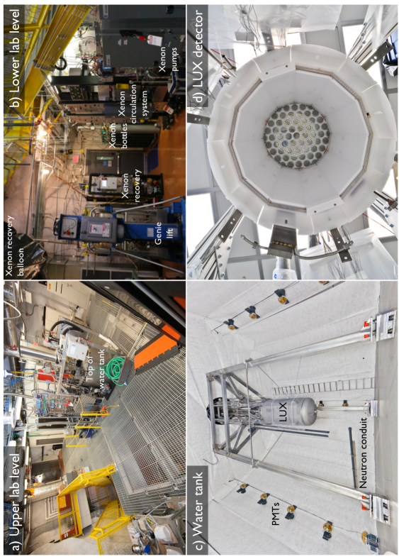
Figure 2.5: The LUX detector. a) and b) Layout of the underground laboratory. c) The inside of the LUX water tank with the PMTs, neutron conduit used for calibrations, acrylic source tubes, and the LUX cryostat. The neutron conduit can move up and down along the side of the cryostat. d) The active volume of the LUX detector with the upper PMT array and the reflective PTFE panels visible.

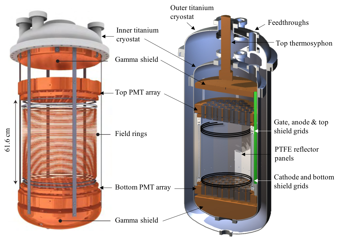
Figure 2.6: Annotated CAD renderings of the LUX detector. Left: LUX detector metal internals supported from the top flange of the inner cryostat. Right: A cross-sectional view of the LUX cryostat. The green line illustrates the path of the cathode HV cable. Figures modified from [190].

The inner LUX cryostat was wrapped in insulating materials and nested inside a larger outer cryostat, both made from low-background titanium [191]. The inner cryostat was $101\,\mathrm{cm}$ tall, $62\,\mathrm{cm}$ in diameter, and contained $370\,\mathrm{kg}$ of LXe with $251\,\mathrm{kg}$ of active mass, where active mass refers to LXe enclosed between the gate and cathode grids and the detector polytetrafluoroethylene (PTFE) walls. The active volume had a shape of a regular dodecagonal prism enclosed by twelve PTFE faces with $47.3\,\mathrm{cm}$ diameter, as measured at -100^∘C between parallel opposite faces. In $z$, the active volume was bounded by the cathode and gate wire grids. This is illustrated in the computer-aided design (CAD) rendering of the detector’s cross section in Figure 2.6.

Given this high-level understanding of the design of the LUX detector, the following sections unpack the inner workings and performance of the individual components.

2.2.1.1 High voltage

In order to establish the electric field needed to drift the S2 electrons, the detector contained five grids in total. The bottommost and topmost grids shielded the bottom and top PMT arrays from the high fields inside the detector. The detector drift field was set by cathode and gate grids separated by $48.3\,\mathrm{cm}$. Between those two grids, to ensure field uniformity inside the active volume, 48 copper field-shaping rings were located behind the PTFE panels as illustrated in Figure 2.6. The rings were separated vertically by $1\,\mathrm{cm}$, and the gate-cathode voltage was graded evenly via a resistor chain. The anode grid was located $1\,\mathrm{cm}$ above the gate grid to create the so-called extraction region [192] held at a high electric field in order to pull electrons out of the LXe and into the xenon gas to create the S2 signal. A detailed description of the grid geometry and detector’s electric fields will be discussed in Chapter 3.

The cathode was biased to a high voltage (HV) to set up electric fields inside the detector. Since HV delivery to liquid noble detectors has been a persistent challenge as will be discussed in Chapter 6, careful design and testing preceded the deployment of the feedthrough. Due to the assembly constraints of the LUX experiment, the cathode HV feedthrough was located outside the detector at the end of a long flexible conduit as shown in Figure 2.7. The feedthrough acts both as a “plug” preventing xenon gas escaping the detector and a connection between the air- and the detector-side cables. The HV feedthrough consists of a conductive cable embedded in a specially designed epoxy-based mass developed at Yale University. The advantage of the feedthrough being located far from the TPC is the ability to use slightly radioactive feedthrough materials, which would not be possible should the feedthrough be located closer to the active LXe volume. This feedthrough was successfully tested up to -100 kV by terminating the distant end of the cable in silicone transformer oil as discussed in great detail in [193]. Despite the feedthrough’s successful tests and its successful performance throughout the LUX era, the detector’s cathode voltage was limited to -10 kV during the scientific dark matter search. This limiting voltage was due to light production from the cathode and gate grids, as discussed in Section 2.4.3.

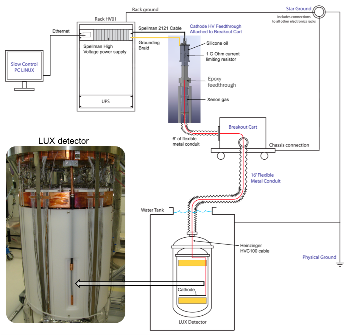
Figure 2.7: LUX cathode high voltage subsystem. A high voltage power supply monitored via the slow control system is fed via an in-house designed feedthrough into the xenon space. The red line indicates the high voltage cable that is submerged in xenon gas until it reaches the main detector volume where it comes down on the side of the detector through a cutout in the ultra-high-molecular-weight polyethylene surrounding the PTFE walls. Figure modified from [193].

2.2.1.2 Light readout

The detector was instrumented with 122 PMTs detecting the primary and secondary scintillation signals. These low-radioactivity PMTs [194] were mounted in copper blocks; 61 were located above the LXe in xenon gas and 61 at the bottom of the detector and submerged in LXe. The PMTs were manufactured by Hamamatsu, model R8778, with a typical quantum efficiency at $178\,\mathrm{nm}$ of 33%. This quantum efficiency includes the probability of photon transmission through the synthetic silica (SiO₂) window, its absorption in the Rb-Cs-Sb bialkali photocathode, and the chance of the photon absorption exciting an electron that gets detected. The PMT dynode chain then amplified the collected electrons to mV-scale signals.

The PMTs were operated with gains of $\sim 4\times 10^{6}$ for an average single photoelectron (sphe) pulse area of $\sim 16\,\mathrm{mV\cdot ns}$ at the PMT output. The analog chain amplification and shaping increase the sphe pulse area to $\sim 151\,\mathrm{mV\cdot ns}$ and full-width (FWHM) of $54\,\mathrm{ns}$ at the digitizer. The PMT response limited the rise time of an S1 pulse to $\sim 6\,\mathrm{ns}$. The effective time constant of the xenon excimer relaxation defined the pulse decay constant. The pulse width of an S2 event varies with depth due to the diffusion of the electron cloud drifting to the top of the detector. More information about the commissioning and performance of the LUX PMTs can be found in [195].

2.2.2 Xenon circulation and cryogenics

Maintaining long electron drift lengths is crucial for proper detector operation. Thus, the detector had stringent requirements regarding xenon purity since electronegative impurities, such as O₂ and N₂, can absorb scintillation light and capture drifting charge thus decreasing the apparent size of the S2 signal. Small quantities of those impurities are present in commercial xenon, but can also be introduced via air leaks and from the continuous outgassing of material inside the detector. Therefore, it is necessary to continuously clean the xenon during detector operations.

Xenon circulation and purification were done in the gas phase since there is not a practical solution for removal of N₂ impurities from liquid xenon. Xenon was liquified in the detector, then evaporated on its way out, purified in the gas phase and recondensed back in the detector. Two double-diaphragm KNF pumps were installed in parallel to achieve a circulation rate of 25 standard liters per minute (SLPM), corresponding to a turnover of xenon of $\sim 229\,\mathrm{kg/day}$. Two additional identical pumps were also obtained so that routine pump maintenance would not interrupt detector operations. The main xenon flow rate was controlled using two Brooks mass flow controllers (MFCs) operating between $1-50\,\mathrm{SLPM}$. Furthermore, four smaller-capacity MFCs were located on purge lines that connect the “dead ends” of detector conduits to the rest of the circulation system to prevent a buildup of dirty xenon gas. A SAES MonoTorr heated zirconium getter operated continuously was used to clean the gaseous xenon from non-noble impurities.

The concentration of impurities in LUX was monitored in two ways. First, the electron drift lifetime was monitored directly by looking at the characteristic S2 pulse size vs. the depth of an event in the detector. Second, the LUX detector had a novel in situ sampling system developed for the LUX and EXO-200 [197] experiments to regularly measure concentrations of impurities in xenon from various parts of the detector (conduits, detector in/out, getter in/out). The sampling system used a liquid nitrogen bath to freeze a small sample of xenon in a U-bend cold trap. The composition of the cold gas above the frozen xenon was then measured with a residual gas analyzer, which provides measurements of minute traces of impurities. The LUX system demonstrated sensitivity to less than 1 part per trillion of krypton and other gasses [198, 199].

LUX used a system of four thermosyphons to maintain xenon in the liquid phase in the detector with exceptional temperature stability. A thermosyphon is a passive gravity-assisted heat exchanger based on convection. The top of the thermosyphon, the condenser, was coupled to a liquid nitrogen reservoir, and the bottom, the evaporator, was in contact with the heat load. Nitrogen condensed at the top and dripped down to the cold head due to gravity. There, it evaporated and rose back up to the condenser, transferring heat from the detector to the liquid nitrogen condenser. In LUX each thermosyphon consisted of a closed system of stainless steel tubing pressurized with gaseous nitrogen. Two of the thermosyphons were able to deliver up to $400\,\mathrm{W}$ of cooling power while the other two in contact with the sides of the detector could deliver up to $100\,\mathrm{W}$ of cooling power. Each cold head was also equipped with a heater to regulate temperature as necessary.

There were three heat exchangers in the xenon circulation path designed to reduce the cooling power needed to condense the xenon. A spillover weir set the LXe level. Liquid from the weir reservoir drained into the evaporator portion of the main heat exchanger HX2 shown in Figure 2.8 depicting detector cryogenics and LXe circulation. HX2 operated in dual phase and consisted of a rectangular evaporator with five vertical tubes that served as a condenser that turned LXe to a cold gas. Next in the path of xenon exiting the detector was heat exchanger HX1, which consisted of two concentric pipes designed to pre-cool the incoming xenon gas by transferring heat to the outgoing cold xenon gas. Finally, HX3 was a long channel engraved in the copper $\gamma$ radiation shield in the bottom of the detector providing further cooling and equalizing the temperature of the incoming liquid to the temperature of the main LXe bath.

In normal circumstances, xenon was stored in eight gas cylinders filled using a compressor. Since the cost of 1 kg of xenon ranges from $\$1,000-\$3,500$, several layers of recovery systems were implemented to avoid xenon loss in case of emergencies. The storage and recovery vessel (SRV) was a high-pressure vessel able to capture the entirety of the LUX xenon. The liquid nitrogen jacket of the SRV was always kept full to enable recovery via cryopumping, and even if all the nitrogen evaporated, the SRV was rated to hold all the xenon at high pressure. In case of a catastrophic failure preventing recovery to the SRV, burst discs and relief devices on the SRV and other parts of the circulation system were connected to a $70\,\mathrm{m^{3}}$ polyester geomembrane recovery balloon with enough volume to store all xenon at low pressure at room temperature. Further details about LUX cryogenics and circulation can be found in [200, 201, 202].

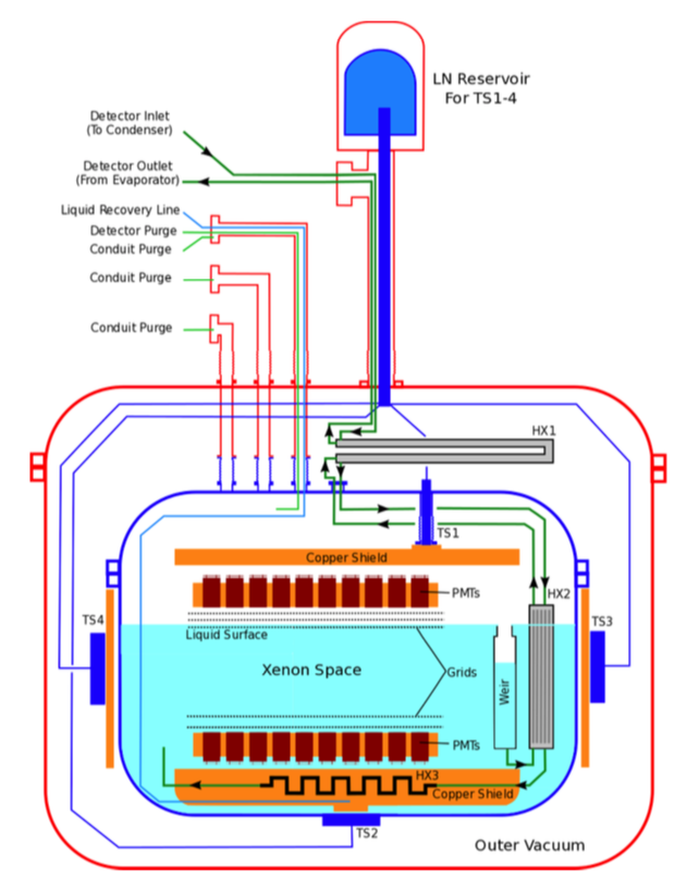
Figure 2.8: Schematics of the cryogenics and xenon circulation inside the detector including cabling, heat exchangers (HX), and conduits for thermosyphons (TS). Bold green lines highlight the main xenon flow path. Figure from [200].

2.2.3 Performance monitoring

The LUX detector was fitted with numerous instruments to monitor and stabilize conditions within the cryostat. Sixty-three $100\,\mathrm{\Omega}$ thin film platinum resistance temperature detectors (RTDs) were used to monitor the temperature in both the inner and outer cryostats. A variety of pressure sensors, manual pressure gauges, and a capacitance manometer were also used throughout the detector. Furthermore, six parallel wire sensors monitored the liquid level; the capacitance of each wire pair depended on the length of wire submerged in the liquid, allowing readout of the overall height of the liquid level. Additionally, three parallel plate sensors were placed 120 degrees apart between the gate and anode grids to ensure liquid surface uniformity across the extraction region. Advantech Adam 6015 modules fed the output voltage of the RTDs, pressure sensors, and level gauges to a slow control database. The slow control system enabled multiple-user access to detector conditions monitoring and automated alarms settings to notify operators of unusual detector behavior. The Automated Controlled Recovery System (ACRS) triggered xenon recovery procedure in case of an emergency.

Throughout the WIMP search, the xenon vessel maintained thermal stability of $\Delta T$ < 0.5 K and pressure stability of $\Delta P<10^{-2}\,\mathrm{bar}$ [163].

2.2.4 Electronics and data acquisition

The LUX data acquisition (DAQ) system was designed to distinguish >95% of sphe at 5 sigma above baseline noise fluctuations and to prevent saturation of events with energies smaller than $100\,\mathrm{keV_{ee}}$. The DAQ can operate with a maximum trigger rate of $1.5\,\mathrm{kHz}$ before incurring dead-time. With 122 PMT channels, each producing 14 bits of data at 100 MHz, the three years of raw data would require 2 exabytes of storage. Therefore, it is crucial to design a triggering system that saves only buffers with information of potential interest. In LUX, the risk of losing valuable data due to a lack of a trigger condition was minimized by digitizing the trigger information alongside the PMT waveforms. To achieve that the PMT readout was split into analog and digital electronics.

Signals from the PMTs were pre-amplified immediately after leaving the xenon space, while post-amplification provided the final signal gain and shape. The signals were summed into 16 groups (8 groups per array) with no adjacent PMTs belonging to the same sum before being split into two copies for the trigger system. One copy of the waveforms was passed through a field programmable gate array (FPGA)-based trigger system (shown as a green data stream in Figure 2.9).

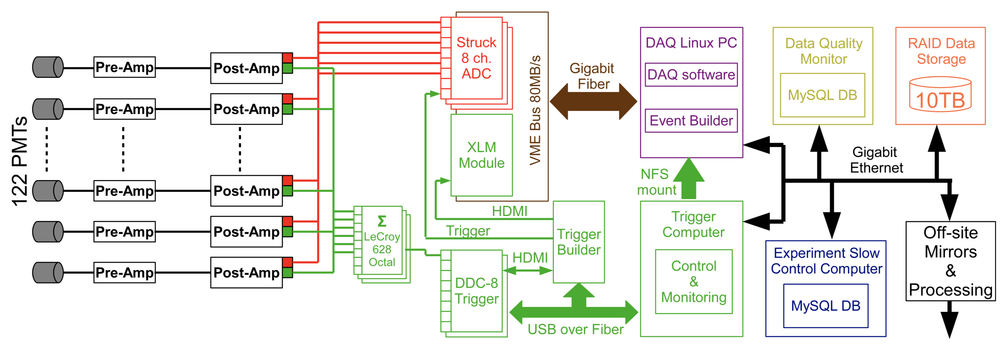
Figure 2.9: Overview of the signal and data processing in LUX. The PMT signals are amplified, shaped and then digitized. Reduced quantities of the trigger system and the waveform data are stored off-line for verification and analysis. Figure from [203].

The second copy was digitized at $100\,\mathrm{MHz}$ by analog to digital converters (ADCs) and written to disk (red data stream in Figure 2.9). In order to manage the required data storage space, the ADCs were controlled by an FPGA that operated in a “pulse only digitization” (POD) mode. In the POD mode, a threshold was set to $1.5\,\mathrm{mV}$ and only pulses rising above this threshold were digitized, thereby rejecting baseline noise. The trigger was applied offline when compressing the raw data into blocks of event-level data. The samples were written to a memory bank from the buffer until an end threshold was reached and a fixed number of samples prior to and immediately following this range were appended. Figure 2.10 shows an example event. Further information about signal and data processing in LUX can be found in [186, 203, 204, 205].

The data went through several stages of refinement. First, the least filtered, un-triggered, raw data for each channel corresponding to ADC memory bank downloads were saved. These data were then built into events where an algorithm collected and saved all PODs occurring within $0.5\,\mathrm{ms}$ of a potential event as determined by the trigger. These triggered, raw data were saved into event-level files and passed on to the data processing stage for analysis.

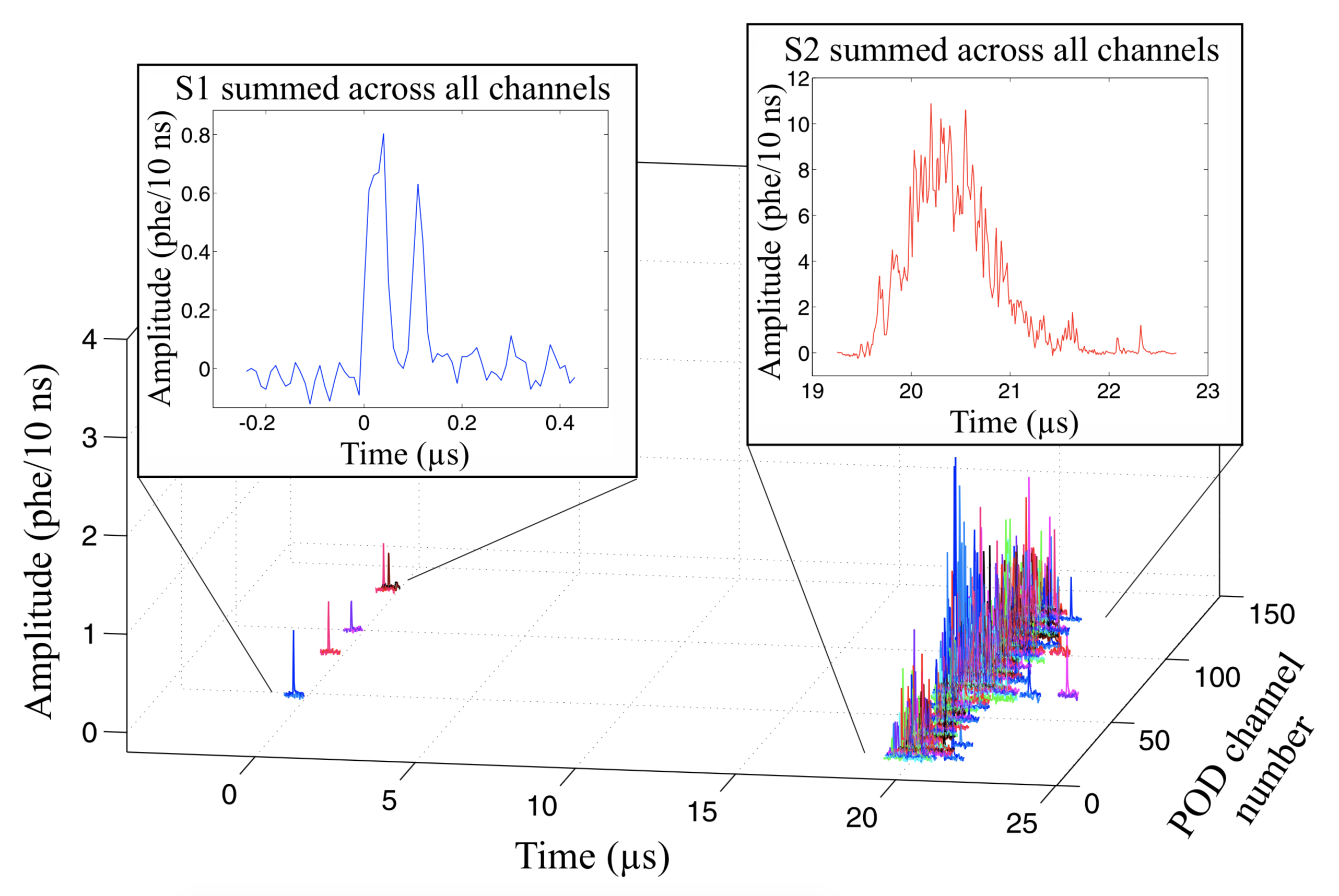
Figure 2.10: Example of a $1.5\,\mathrm{keV_{ee}}$ low-energy event as seen in raw data. Each POD channel number corresponds to an individual PMT. Figure from [203].

2.2.5 Data processing

The LUX data processing framework (DPF) extracted essential information from the event-level files and saved the output as reduced quantities (RQs). These RQs include information about the number of identified pulses, trigger timestamp, pulse information, etc. Thanks to the modular nature of the DPF, the list of modules used for individual data processing runs can be easily swapped in and out. The list of modules used with their specific configurations and calibration constants were provided to the framework and stored in a MySQL database (called LUG) and associated with a unique identifier. This ensured that data for any particular analysis were processed with the same settings. The stored detector calibration constants included PMT gains, $\left(x,y,z\right)$ spatial calibration maps for S1 and S2 pulses, electron lifetime, light response function for position reconstruction, and more.

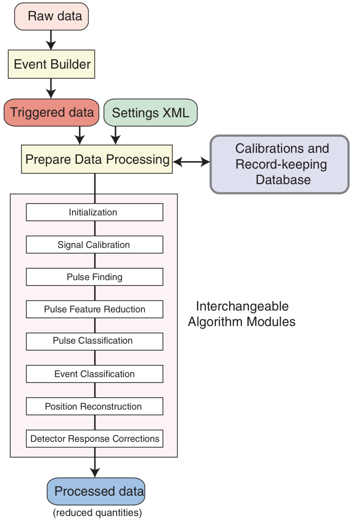
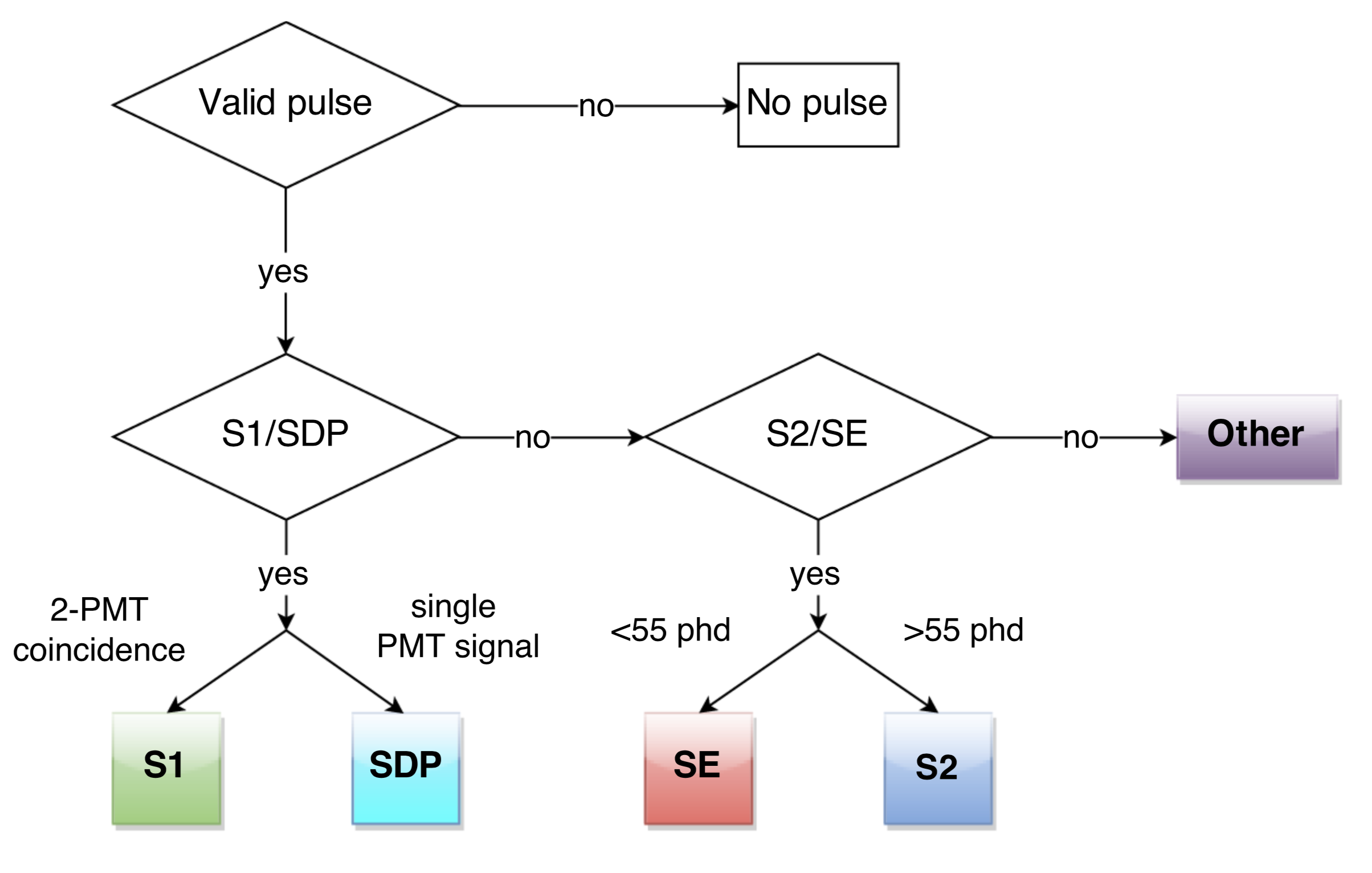
Figure 2.11: Left: Schematic view of the LUX Data Processing Framework. Right: Pulse classification decision tree. Figures from [186].

Figure 2.11 shows a schematic representation of the journey of raw data from the DAQ to the reduced quantities used in higher level analyses. The primary goal of the RQs is to find and identify different valid pulses in the acquired waveforms to be used in future analyses. A sliding boxcar filter finds and separates S1-, S2-, and other-type pulses returning their start and end times. Figure 2.11 illustrates the decision tree used for pulse classification. A two-PMT coincidence is required for an S1 signal in order to reject photons from spontaneous PMT photocathode emission. An S2-type signal needs to be larger than 5 phd and can be further classified into single electrons (SE) or S2 signals. The event type of interest for the WIMP search analysis is a single scatter, or “golden,” event; this type of event is required to have a single valid S1 signal followed by a single S2 signal with at least 55 phd in size. About 95% of triggers are rejected by the golden event requirement. An extensive hand-scanning campaign was conducted to cross-check the efficacy of the gold event filter. Further information about the LUX DPF can be found in [186, 206].

2.2.5.1 Position reconstruction

The $\left(x,y\right)$ position of an event in the LUX detector is recovered from the light of the electroluminescent S2 signal collected by the individual PMTs in the top array. For the position reconstruction, an algorithm called Mercury was used, originally developed for the ZEPLIN-III dark matter experiment [207]. It is a statistical-based algorithm that uses a maximum likelihood test. It uses an empirical light response function (LRF) to characterize the response of each PMT as a function of the position of photon emission. A major advantage of this method is that it only needs measured data obtained from in situ calibrations (rather than simulations) to recover the position of interactions.

Due to the presence of PTFE reflectors around the detector volume, the LRFs were implemented as a sum of two terms: an axial component describing the light going to the PMT either directly or via a reflection from the liquid surface and a polar component characterizing the light reflected from the PTFE walls. This resulted in an observed position resolution of $0.097\pm 0.003\,\mathrm{cm}$ for pulses with an average area of 22,000 phd and $2.24\pm 0.04\,\mathrm{cm}$ for sphe. Figure 2.12 illustrates the performance of the position reconstruction software using on $\mathrm{{}^{83m}Kr}$ calibration data.

The time difference between the S1 and the S2 pulses provides information about the event depth. In WS2013, where WS stands for WIMP Search, the conversion between drift time and $z$ position was calculated assuming a uniform and constant electric field in the active volume, using electron drift velocity $v_{d}=0.1518\pm 0.0011\,\mathrm{cm/\mu s}$ [186]. In WS2014-2016 I developed electric field maps as discussed in Chapter 3 were used for this conversion. Further details about the position reconstruction can be found in [208].

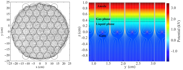
Figure 2.12: Left: A scatter plot of reconstructed $\left(x,y\right)$ positions of uniformly distributed $\mathrm{{}^{83m}Kr}$ calibration data for drift times between $4-10\,\mathrm{\mu s}$. Details about $\mathrm{{}^{83m}Kr}$ are described in Section 2.2.6.1. Black lines represent the PMTs and TPC inner walls. A striped pattern with the pitch of gate grid wires is visible. Figure from [208]. Right: Electric field simulation of gate regions showing grids wires concentrating electron trajectories (gray lines) into tights bands resulting in the effect shown on the left. The black line illustrates the liquid level. Note that the field line density does not illustrate field strength.

2.2.5.2 S2 coordinate system

The 3D position reconstruction of ionization vertices requires an understanding of the electrons’ path from the interaction site to the point of detection in xenon gas. As described above, the $\left(x,y\right)$ position of an event in the detector is reconstructed using the Mercury algorithm from the electroluminescence of the S2 signal in gaseous xenon at high field. If the fields were perfectly perpendicular to the liquid surface at all positions, the location of the event as seen by the top PMT array and the real event location would be identical. Although the field is mostly perpendicular to the liquid surface, it is not perfectly the case everywhere. A non-zero radial component, inducing a radially-inward electron drift, affects drifting electrons. This radial component is due to the non-zero electrostatic transparency of the field cage and field grids as will be discussed in detail in Chapter 3.

Therefore, there are two different coordinate systems used in the analysis: the real coordinates and the S2, or reconstructed, coordinates. The S2 coordinates ($x_{S2},\,y_{S2},\,\mathrm{drift\,time}$) represent the event position as seen by the top PMT array with the event depth given by the electron drift time. In these coordinates, all active volume events have a slightly distorted edge as shown in Figure 2.13 due to field non-uniformities. A field correction needs to be applied to translate the S2 coordinates into the real space $\left(x,\,y,\,z\right)$ coordinates. As described above, this was trivial in WS2013. However, due to changing electric fields in WS2014-16, a special position reconstruction algorithm was developed to map the Mercury algorithm coordinates into real space coordinates using electric field models discussed in Chapter 3.

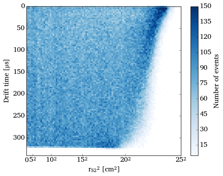
Figure 2.13: 2D histogram showing the reconstructed position of $\sim 650,000$ uniformly distributed $\mathrm{{}^{83m}Kr}$ events in the active volume of the LUX detector as a function of $r_{S2}^{2}$. This data comes from a $\mathrm{{}^{83m}Kr}$ injection during WS2013 on 2013-05-10. The higher event density in the upper right corner comes from a systematic error in the Mercury algorithm in reconstructing events with low drift time at high radius near the outermost PMT. This false artifact produced by the Mercury algorithm is well known, far away from the fiducial volume, and accounted for in analyses.

2.2.6 Calibrations

A thorough characterization of particle interactions in the active detector region is key to correctly identifying possible dark matter particles. In LUX the primary goal is to identify unambiguous NR signals composed of single-site scatters homogeneously distributed in the active volume. It is essential to correctly identify NR interactions in the detector and distinguish them from ERs. To achieve this, LUX pioneered a number of novel calibration methods that were employed extensively before, during, and after the scientific runs. Spectral and monoenergetic sources, both internal and external, were used to measure the detector’s ER and NR response.

The self-shielding ability of LXe that makes it such a great dark matter target causes challenges during calibrations. Photons with energies below the MeV scale are strongly attenuated in LXe as shown in Figure 2.2, and therefore external $\gamma$ sources can only be used to calibrate the outer couple of centimeters of LXe. Furthermore, high energy $\gamma$-rays such as the ones from ¹³⁷Cs are very likely to produce multiple-site scatters; single-site scatters can be produced with $\sim 1-10\,\mathrm{keV}$ energy deposition but only if the outgoing $\gamma$ can escape the detector’s active volume without any further scatters. During such a calibration, the detector is swamped with edge events, causing saturation effects due to the high event rates and making external $\gamma$-rays not particularly useful for fiducial volume calibrations.

However, $\gamma$ ray calibration sources are useful for position reconstruction and background studies since they so strongly illuminate detector walls. To that end, LUX had six air-filled acrylic source tubes that extended down from the top of the water tank flush against the sides of the outer cryostat as illustrated in Figure 2.5. Radioactive sources were deployed and retracted by a system of pulleys [202]. Gamma-ray sources ⁵⁷Co ($122\,\mathrm{keV}$ $\gamma$), ⁶⁰Co ($1,173\,\mathrm{keV}$ and $1,332\,\mathrm{keV}$ $\gamma$s), ¹³⁷Cs ($662\,\mathrm{keV}$ $\gamma$), and ²²⁸Th ($2,614\,\mathrm{keV}$ $\gamma$) were all available for ER response calibration via the source tubes.

For NR calibrations, AmBe (mix of an alpha-emitting ²⁴¹Am + ⁹Be with a mean energy of 4.2 MeV and maximum neutron energy of 11 MeV) and ²⁵²Cf (emitting neutrons from spontaneous fission emitting) were deployed in the source tubes. Later, calibrations were performed using a deuterium-deuterium neutron beam generator located outside the water tank was used to calibrate the LUX detector response as discussed in Section 2.2.6.3. The latter method is preferable due to timing control over neutron emission and the mono-energetic nature of the source.

However, the best way to calibrate ER events is by using radioactive sources introduced to the active xenon volume itself. This runs counter to the instinct of any reasonable dark matter detector operator due to worries of LXe contamination. Therefore, the radioactive sources introduced to the detector’s active volume must be either short-lived isotopes that will decay away rapidly or sources bound to a molecular form that can be efficiently extracted by the getter and not halt the dark matter search. LUX employed two such internal calibration sources: a nearly monoenergetic metastable isotope of krypton, $\mathrm{{}^{83m}Kr}$, and a low-energy beta decay isotope ³H, in the form of tritiated methane CH₃T.

The internal source gases were introduced from a controlled, measured volume via plumbing into the gas system circulation using a pressure differential in the main xenon flow. Once condensed, the radioactive isotopes mixed uniformly within the detector’s active volume within minutes as illustrated in the time lapse plots in Figure 2.14.

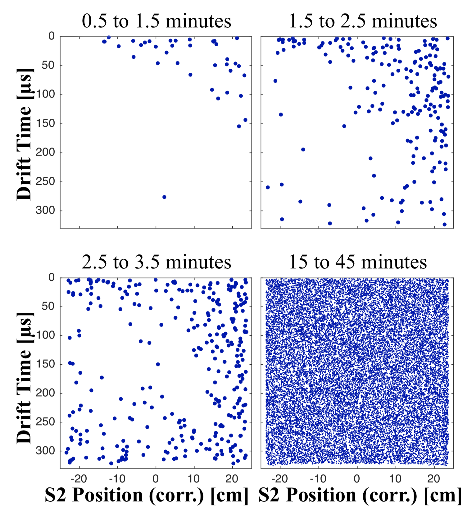
Figure 2.14: Positions of reconstructed $\mathrm{{}^{83m}Kr}$ event vertices in four distinct time windows selected from a thin vertical slice in the detector. Initially, a large scale clockwise flow is observed along with turbulent mixing ($0.5-3.5$ minutes) until $\mathrm{{}^{83m}Kr}$ becomes uniformly distributed in LXe 15 minutes after injection. Figure from [209].

2.2.6.1 Metastable krypton-83 ($\mathrm{{}^{83m}Kr}$)

The metastable isotope of krypton-83, $\mathrm{{}^{83m}Kr}$, is a radioactive element with a half-life of 1.86 hours that decays into its ground state by emitting a 32.1 keV followed by a 9.4 keV conversion electron 154.4 ns later. Both of these transitions can occur in various ways as illustrated in Figure 2.15, but most often they result in an internal conversion (IC) followed by an emission of an Auger electron. Additionally, $\mathrm{{}^{83m}Kr}$ decay can also result in an emission of an x-ray or a $\gamma$-ray, with a maximum photon energy of 12 keV. Since it is also a noble gas, krypton is not removed by the getter. However, in its ground state, $\mathrm{{}^{83}Kr}$ is not radioactive and only tiny quantities are introduced into the detector during calibrations which do not present any problem to the overall detector performance. LUX has made extensive use of $\mathrm{{}^{83m}Kr}$ for calibration purposes. Due to its inert nature and keV-scale decay energy, it is a natural choice for calibrating liquid noble detectors. Furthermore, the short half-life allows for a quick return to baseline trigger rate following injection and since its total transition energy is well above the range for WIMP scatters the risk of contaminating the search region is avoided.

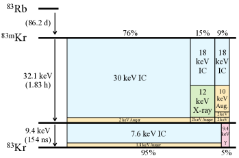
Figure 2.15: Decay scheme of $\mathrm{{}^{83m}Kr}$. The width of each column is proportional to the branching fraction of that decay mode. Energy is partitioned between internal conversion electrons (blue), Auger electrons (yellow), x-rays (green), and $\gamma$-rays (red). Figure from [209].

$\mathrm{{}^{83m}Kr}$ was first used as a calibration source in high energy and heavy ion detectors [210, 211, 212, 213] and in experiments measuring the endpoint of tritium spectrum [214, 215, 216, 217]. Initial demonstrations of $\mathrm{{}^{83m}Kr}$ injection and calibration technique in liquid xenon, liquid argon, and liquid neon were performed at Yale University [218, 219, 220] with subsequent studies performed in other detectors [221, 222]. The LUX detector was the first to use $\mathrm{{}^{83m}Kr}$ for calibrations of a dark matter experiment [209]. The source used in the LUX detector was made using ⁸³Rb produced in a proton beam at Oak Ridge National Laboratory [223], deposited on charcoal at Yale and inserted into the LUX injection system at SURF. Since ⁸³Rb decays to $\mathrm{{}^{83m}Kr}$ with an 86.2 day half-life, several sources were manufactured during LUX operations. Typical injections were $\sim 10\,\mathrm{Bq}$, but depending on the need the amount injected could be higher ($\sim 100\,\mathrm{Bq}$) or lower.

Figure 2.16 shows a selection of $\mathrm{{}^{83m}Kr}$ events in the LUX detector remaining after very loose data cuts were applied. The selected events contain either 1 or 2 S1 signals at most $10\,\mathrm{\mu s}$ apart happening before an S2 pulse. The corrected S1 pulse area is constrained to $100<\mathrm{S1\,phd}<370$ and the S2 uncorrected pulse area is constrained by $100<\mathrm{S2\,phd}<50,000$.

Figure 2.16: Selection of $\mathrm{{}^{83m}Kr}$ calibration data in LUX from 2016-08-17 after cuts have been applied.

$\mathrm{{}^{83m}Kr}$ was used as a “standard candle” in LUX. There were $\sim 10^{6}$ $\mathrm{{}^{83m}Kr}$ events injected weekly. Krypton atoms mix homogeneously with LXe making $\mathrm{{}^{83m}Kr}$ a perfect candidate to use in developing 3D maps of the electric field in the detector’s active volume, position-dependent pulse-area corrections, field corrections, and more. The application of $\mathrm{{}^{83m}Kr}$ for development of field maps of the LUX detector will be discussed in great detail in Chapter 3.

Pulse-area corrections

S1 photon detection efficiency varies primarily with event depth, which needs to be corrected for in the analyses. S1 photons emitted near the bottom PMT array are $\sim 50\%$ more likely to be detected than those originating near the liquid surface due to the total internal reflection of scintillation photons at the liquid-gas interface. Hence the same number of initial photons will produce a different S1 signal size in the PMT arrays. Figure 2.17 shows this $z$ dependence on event location. To map this efficiency, the $\mathrm{{}^{83m}Kr}$ S1 amplitude is found for each bin in $\left(x_{\mathrm{S2}},\,y_{\mathrm{S2}},\,t_{\mathrm{S2}}\right)$ and a 3D S1 correction map is constructed as the inverse of these amplitudes, normalized to the detector center at $\left(0\,\mathrm{cm},\,0\,\mathrm{cm},\,159\,\mathrm{\mu s}\right)$. The efficiency-correction map is then applied as a linear interpolation on the 3D grid. Since S1 correction maps did not vary much with date a single large $\mathrm{{}^{83m}Kr}$ injection was used for the entire WS2013. WS2014-16 required additional calibration data due to varying electric fields.

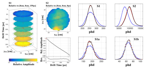
Figure 2.17: Left: Maps of relative variation of $\mathrm{{}^{83m}Kr}$ S1 and S2 amplitudes as derived from injection on May 10, 2013. The S1 and S2 amplitudes share the same color scale. Also shown is the 1D $z$ map correcting for electron lifetime. The $z$ correction has an exponential fit (in gray) with $\tau_{e}=805.2\,\mathrm{\mu s}$. The red circles in each plot represent the normalization points. Right: The effect of applying the S1 and S2 amplitude corrections. The uncorrected data is shown in blue; areas corrected for $z$-dependence variation is shown in red; areas corrected in all three spatial coordinates are black. The top row treats the two S1 pulses as a single pulse with $\mathrm{t_{sep}<1.2\,\mathrm{\mu s}}$. The bottom row shows the individual S1 peaks used $\left(\mathrm{t_{sep}>1.2\,\mathrm{\mu s}}\right)$ as a cross-check for S1 corrections. It can be seen that a full 3D correction represents only a marginal improvement over a $z$-only correction. Figures from [209].

For S2 pulse corrections, the $z$ and $\left(x,y\right)$ position corrections are applied independently. The $z$ dependence results from electron capture on electronegative impurities while drifting. This correction is a simple exponential fit normalized to unity at the liquid surface as illustrated in Figure 2.17. The correction is interpolated smoothly between $\mathrm{{}^{83m}Kr}$ injections.

Non-uniformities of the S2 signal in the $\left(x,y\right)$ plane are due to variations of the liquid surface, a slight tilt of the detector, and bowing or sagging of the wire grid plane. The corrections are constructed by binning $\mathrm{{}^{83m}Kr}$ data on an $\left(x,y\right)$ grid and finding average S2 amplitudes for each 2D bin normalized to the center of the liquid surface.

Field variations using S1a:S1b ratio

As shown in Figure 2.15, $\mathrm{{}^{83m}Kr}$ proceeds through two back-to-back transitions. Because the S2 signals have FWHM of $1.0-1.9\,\mathrm{\mu s}$ depending on $z$ position, the two decay steps are merged in the relatively broad S2 signal. Due to the short S1 pulse width ($\sim 100\,\mathrm{ns}$) a significant fraction of $\mathrm{{}^{83m}Kr}$ S1 pulses are detected individually in the PMT array. Those two S1 pulses are referred to by their ordering as S1a (32.1 keV) and S1b (9.4 keV). The S1a and S1b pulses can be used to study the dependence of electron-ion recombination on the electric field. A weaker field allows more recombination, enhancing the S1 signal and proportionally suppressing the S2 signal, while a higher field has the opposite effect. The ratio of the two S1 amplitudes varies with field alone since any detector gains and efficiencies affect both amplitudes equally causing the S1b/S1a ratio to increase with the electric field. This ratio technique for field amplitude measurement was used in WS2014-16, where the field variations in $\mathrm{{}^{83m}Kr}$ recombination were more substantial and required careful treatment.

Further details about the LUX $\mathrm{{}^{83m}Kr}$ calibration techniques can be found in [209, 224].

2.2.6.2 Tritium (³H)

Tritium has a 12.3 year half-life and $Q$ value $Q=18.6\,\mathrm{keV_{ee}}$. Its mean energy is $5.6\,\mathrm{keV_{ee}}$, and the beta energy spectrum has a broad peak at $2.5\,\mathrm{keV_{ee}}$ both of which have a significant overlap with the WIMP NR range, so it is perfectly tailored to the calibration of electron recoils of a dark matter detector.

³H was introduced into the detector as tritiated methane gas CH₃T and was mixed within the detector’s active volume on a similar timescale as $\mathrm{{}^{83m}Kr}$. The source was prepared by an external vendor with an activity of $3.7\,\mathrm{MBq}$ per millimole and inserted into the circulation in a 2.25-liter stainless steel bottle mixed with 2 atmospheres of LUX-quality purified xenon. Prior to the first injection, the ability of the LUX getter to efficiently remove CH₃T from xenon gas was verified to prevent absorption into plastics in the detector due to its long half-life.

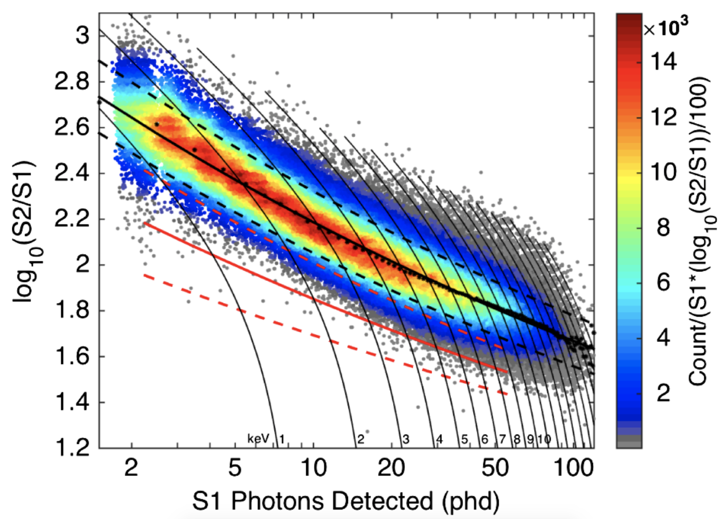
Figure 2.18: The LUX electron recoil band illuminated by ³H events at 180 V/cm. The tritium data is shown as a scatter plot in $S1$ vs. $\log(S2/S1)$ space with contours of constant ER energy (solid gray lines). Measured Gaussian means in each S1 bin are shown with an empirical power line fit (solid black line) along with the 10 and 90% contours (dashed black lines). Also shown is the equivalent NR band mean (solid red line) along with the 10 and 90% contours (dashed red lines) obtained from deuterium-deuterium neutron generator data discussed in Section 2.2.6.3. Figure from [182].

CH₃T was injected into the detector several times throughout its operation to characterize the detector’s ER response. This is critical for correct mapping of the LUX background model to the signal parameter space for analysis since the dominant background for the WIMP search is leakage of ER events into the NR band in the $S1$ vs. $\log(S2/S1)$ space as illustrated in Figure 2.18. Figure 2.19 shows the observed spectrum in $n_{e}-n_{\gamma}$ space as measured by LUX using 170,000 ³H decays recorded in the fiducial volume after the WS2013 dark matter search. Also shown is the total number of electrons and scintillation photons after recombination as a function of energy. Above 4 keV the number of electrons drops below the number of photons, which is consistent with a substantial recombination effect at these energies and an electric field of 180 V/cm. The tritium spectrum as measured by the detector and the ratio of the data to the smeared theoretical spectrum is shown in Figure 2.20, along with an empirical fit to an error function. The effective 50% energy threshold for ER events was found at $1.24\pm 0.026\,\mathrm{keV}$. Further details about the LUX ³H calibration technique can be found in [182, 224, 225].

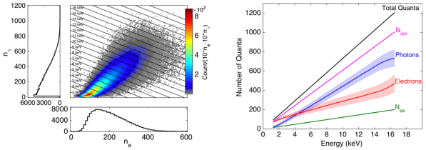
Figure 2.19: Left: Scatter plot of $n_{e}$ vs $n_{\gamma}$ for 170,000 fiducial tritium events at 180 V/cm as measured by LUX. Lines of constant energy according to Equation 2.14 are shown assuming $W=13.7\,\mathrm{eV}$. Right: The underlying mean number of quanta responsible for the shape of the ER band in LUX at 180 V/cm. The bands indicate the correlated systematic errors on $g_{1}$ and $g_{2}$. Figures from [182].

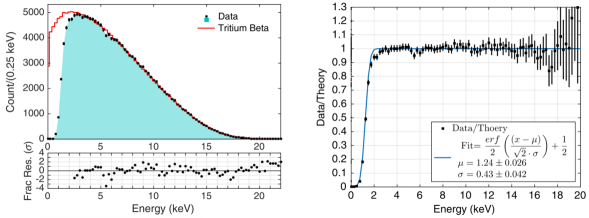
Figure 2.20: Left: Tritium energy spectrum from LUX (black) compared to a theoretical tritium spectrum convolved with detector resolution (red) $\nicefrac{{\sigma_{E}}}{{W}}=\sqrt{\sigma^{2}\left(n_{\gamma}\right)+\sigma^{2}\left(n_{e}\right)}$. The cut off of the data on the left is due to a finite detector resolution at low energies. Right: Ratio of measured tritium energy spectrum (black data) and the theoretical one (blue line) for the same dataset. A fit to an error function is also shown. Figures from [182].

2.2.6.3 Deuterium-deuterium (DD) neutron beam

Calibration of the NR response was accomplished with the scattering of 2.45 MeV neutrons sourced by a deuterium-deuterium (DD) neutron fusion generator. An Adelphi Technology, Inc. DD108 generator was located outside the water tank. A collimated beam of neutrons was fired through an air-filled conduit suspended in the water to penetrate the LXe space. The conduit is visible in Figure 2.5 and could be raised or lowered alongside the detector to enable calibrations at various $z$. The generator works by accelerating deuterium ions into a deuterium-loaded target. To achieve a monoenergetic beam, only neutrons emitted at a $90^{\circ}$ angle relative to the incoming deuterium are selected from the ²H(d,n)³H fusion reaction. The air-filled conduit results in a tightly collimated beam visible in the detector as shown in Figure 2.21. Visible closer to the wall are neutron events that have scattered outside of the TPC and contaminate the monoenergetic data selected by the black dashed box.

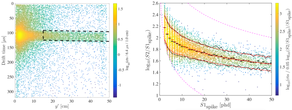
Figure 2.21: Left: Spatial distribution of single-scatter events from DD calibration where $y^{\prime}$ axis is parallel to the direction of the neutron beam. The neutron beam pipe is aligned at $107\,\mathrm{\mu s}$. Black dashed rectangle selects for monoenergetic scatters inside the fiducial volume. A 12.6 cm total mean free path for neutrons makes it more probable for a neutron to exit out of the top of the xenon volume than the bottom. This plot contains the full 107.2 live-hours of 2013 DD data. Right: The LUX nuclear recoil band (black line) and the corresponding Gaussian fit mean value for the simulated NR band (red line). The 10 and 90% contours are also shown for data (dashed black) and simulation (dashed red). Figures from [226].

The collimated monoenergetic neutrons arriving to the TPC can scatter off xenon nuclei with a known angular distribution and deposit varying amounts of energy. Even though the two S1s from the interactions overlap, the two S2 signals can be resolved if they are sufficiently separated in $z$. This can be leveraged for measurements of neutron charge and light yields in the detector. The charge yields are calculated first by selecting for double scatter events where the reconstructed vertex position enables calculation of the scattering angle at the first interaction site. This kinematically constrains the deposited energy of the first nuclear recoil, enabling the ionization yield to be measured as a function of nuclear recoil energy from 0.7 to 24.2 keV_nr. With this measurement, single-scatters can be used to determine the light yield. In LUX the light yield was measured as a function of recoil energy between $0.7-74\,\mathrm{keV_{nr}}$. Figure 2.21 shows the NR band of the LUX detector found both from data and simulations. Further details about the LUX DD calibration technique can be found in [226, 227].

2.3 Simulations and backgrounds

The LUX detector is sufficiently complex that a deterministic model would require excessive computational resources. However, Monte Carlo simulation methods with appropriate constraints generate the required statistical confidence needed to achieve a thorough understanding of the detector. This starts by modeling the detector itself; this model is then used to simulate particle interactions that are used to simulate signal and background models for the final analysis. In LUX, the Geant4-based [228] LUXSim [229] software package was used featuring a very detailed reconstruction of the LUX detector geometry inside the water tank based on CAD designs. Energy deposits from particle interaction in LXe were then used to model the production of VUV scintillation photons and ionization electrons. These light and charge yields were modeled with the Noble Element Simulation Technique (NEST) [230, 231], a semi-empirical collection of models based on past detector calibration data. Finally, full ER and NR simulations datasets were created and passed through the data-processing chain to provide estimates of the expected WIMP NR signals and the predicted background spectra. Those were then used in the probability density functions (PDFs) used in the profile likelihood ratio analysis. Further details about the use of LUXSim in LUX analysis can be found in [186].

Due to the rare-event nature of the search, minimizing backgrounds was one of the primary concerns during detector design and construction. There are several groups of backgrounds discussed in the remainder of this section. Further details about both ER and NR backgrounds are described in [186, 232].

ER backgrounds:

ERs dominated backgrounds: the main sources were Compton scattering $\gamma$-rays from detector components, and $\beta$ and electron-capture decays within the LXe target. The bulk of the events originated in the detector materials, such as products from the decays of ⁴⁰K, ⁶⁰Co, and the many radioisotopes of the uranium and thorium chains that emit high-energy $\gamma$-rays that can Compton scatter once in the fiducial volume and leave. Other backgrounds arise from the xenon target itself: $\beta$ decay backgrounds from ⁸⁵Kr (remaining in xenon after purification) and ²¹⁴Pb (a radon daughter), and electron capture decays of ¹²⁷Xe and ³⁷Ar. ¹²⁷Xe is created while xenon is exposed to cosmic rays and thermal neutrons on the surface, but thanks to its half-life of 36 days ¹²⁷Xe was a significant source of backgrounds only during WS2013, where it was also used for low-energy ER calibrations [233].

NR backgrounds:

NR backgrounds arise from ($\alpha$, n) reactions or from cosmogenic muon interactions in the water or cavern rock, but provide only a minimal background for the search. Results from an extensive radioactivity screening campaign with high-purity germanium detectors and neutron activation form the LUX background model, providing input into the Monte Carlo simulations. Figure 2.22 shows the measured $\gamma$ ray spectrum in the LUX active volume with identified peaks and the observed distribution of low-energy background events in WS2013.

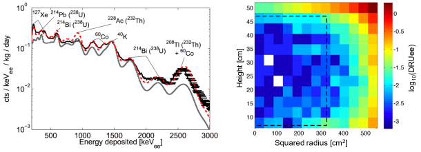
Figure 2.22: Left: Measured $\gamma$ spectrum in the LUX active volume without the top and bottom 2 cm (black) including both single- and multiple-scatters. Two simulations spectra are also shown: a spectrum based on counting measurements alone (gray) and a spectrum with best-fit scaling for ²³⁸U, ²³²Th, ⁴⁰K, and ⁶⁰Co decays (dashed red). Right: LUX $\gamma$ ray ER background density in the range $0.9-5.3\,\mathrm{keV_{ee}}$ ($\sim 2-30\,\mathrm{phe}$) as a function of position from measured data. Rates are in units of log₁₀(DRU_ee) where DRU is the differential rate unit of $\mathrm{events\cdot kg^{-1}\cdot day^{-1}\cdot keV_{ee}^{-1}}$. The 118 kg fiducial volume used in the WS2013 is overlaid as the black dashed contour. Figures from [232].

Wall backgrounds:

Further backgrounds arise from interactions occurring very close to the detector’s PTFE wall, referred to as “wall events.” These events can exhibit a loss of charge to the PTFE, which results in a low $\log_{10}(S2)$. In theory, these backgrounds should be excluded by the fiducial cut, but due to the limited accuracy of position reconstruction, some of these events statistically leak into the search region. Empirical estimates are calculated using control samples of the data and included in the background model. A detailed discussion of these backgrounds can be found in [206, 234, 235].

Random coincidence backgrounds:

Random coincidence of unrelated S1-only and S2-only events can generate apparent WIMP-like events. The isolated S1 rate from threshold to 50 phd is 1 Hz. This leads to a prediction of 1.1 background events in the 95 days of WS2013 [186].

Neutrino backgrounds:

Another background for WIMP detectors without directional sensitivity are two kinds of neutrino interactions: $\nu-e^{-}$ neutral current elastic scattering, where the neutrino interacts with atomic electrons, and $\nu-A$ neutral current coherent elastic scattering, where the neutrino interacts with the target nucleus [236, 237] (observed recently for the very first time [238]).

Neutrino-electron scattering contributes to ER backgrounds. It is dominated by low energy neutrinos, such as $pp$ solar neutrinos, with contributions from the ⁷Be and CNO chains. Coherent elastic neutrino-nucleus scattering results in NR background. At low WIMP masses, ⁸B and $hep$ solar neutrinos are expected to contribute the most background events, while at masses above $20$ GeV/c² contributions from diffuse supernova neutrinos and atmospheric neutrinos will dominate [104].

Fortunately, in LUX these interactions are expected to have produced only $\sim$ 0.1 detectable NR events in the full exposure [187]. However, these will become an obstacle for the increasingly large next-generation dark matter detectors, such as LZ.

2.4 LUX WIMP search results

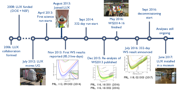
Figure 2.23: LUX timeline. References to results published in Physical Review Letters (PRL) are indicated below the limits plots.

Name	Date	Goal
Run1	Early 2011
	First detector cool down with argon gas in the surface lab
Run2	Late 2011
	Full systems test in the water tank in the surface lab
Run3	April 24, 2013 -
September 1, 2013	WS2013, 95 live-days, in Davis Cavern
Run4	September 11, 2014 -
May 2, 2016	WS2014-16, 332 live-days, in Davis Cavern

Table 2.2: Overview of LUX data taking periods. Details regarding the detector assembly, Run1, and Run2 can be found in [195]. A grid conditioning campaign took place during an engineering run between Runs 3 and 4 in spring 2014 in the Davis Cavern.

After the tremendous effort that was put into the LUX detector design, assembly, and commissioning, the LUX detector began taking WIMP search data in 2013 and continued its scientific quest until fall 2016 when it was disassembled to make space for the LUX-ZEPLIN (LZ) dark matter detector and moved to a museum exhibit at the Sanford Lab visitor center in Lead, SD. Despite not finding WIMPs, the LUX operations were a success. The absence of a dark matter signal combined with its edge-cutting sensitivity enabled LUX to place world-leading exclusion limits on WIMP properties. Exclusion limits are helpful for theoretical modeling, evaluating past detection claims of dark matter, and informing the next generation of dark matter experiments. LUX also pioneered many novel calibration techniques now used commonly in the field. Furthermore, the expertise developed by the LUX experiment provides beneficial know-how for the design and construction of the next-generation of dark matter detectors.

Figure 2.23 shows the timeline of the LUX experiment. Before starting the main scientific dark matter search, the detector was commissioned on the surface to ensure all systems were adequately operating before the detector was sealed and moved underground. An overview of the four main scientific runs is illustrated in Table 2.4. Data used for the main dark matter search analysis were collected over two scientific runs - Runs 3 (WS2013) and Run4 (WS2014-16), which led to the publication of three primary WIMP search results discussed below. These are limits on isospin-invariant SI coupling as this is the WIMP scenario that the LUX detector is the most sensitive to. Additionally, scientific results for various other types of dark matter have been published.

2.4.1 Profile likelihood ratio

To claim a discovery or place a limit, a frequentist significance test using the profile likelihood ratio (PLR) statistic was used, a common choice among many recent particle physics experiments. The following discussion provides a high-level overview of this topic. For a more in-depth treatment consult References [206, 239, 240, 241, 242] that were used to compile this section.

A hypothesis $H$ is a statement about the probability for the data, often written $P\left(x|H\right)$. For purposes of discovering a new signal, the WIMP signal plus background model constitutes the null hypothesis $H_{0}$, which is tested against an alternative background-only hypothesis $H_{1}$. In this context the null hypothesis is the test hypothesis since one is trying to test the presence of a signal with strength parametrized by $\sigma$, trying to reject it at a specified confidence limit (CL). In the analysis, $H_{0}$ and $H_{1}$ are a suite of Monte Carlo pseudo experiments generated using modeled backgrounds ($H_{1}$) and backgrounds with an expected signal ($H_{0}$). To set a limit, an acceptance region in data space $\mathbf{x}$ is defined that contains 90% of experiments under $H_{0}$. The signal model $H_{0}$ is rejected when the observed data falls outside that region.

If the probability $P\left(\mathbf{x}|H\right)$ for data $\mathbf{x}$ is regarded as a function of the hypothesis $H$, it is called the likelihood of $H$, written as $\mathscr{L}\left(H\right)$. Often the hypothesis is characterized by one or more parameters $\theta$, in which case $\mathscr{L}\left(\theta\right)\equiv P\left(\mathbf{x}|\theta\right)$ is called the likelihood function.

A region of data space $\mathbf{x}$, called the acceptance region $w$, is specified such that there is no more than a given probability $\alpha$ under $H_{0}$, called the confidence level of the test, to find $\mathbf{x}\in w$. If the data are observed in the acceptance region, $H_{0}$ is rejected. To maximize the power of a test of $H_{0}$ with respect to the alternative $H_{1}$, the Neyman-Pearson lemma [243] states that the acceptance region $w$ should be chosen such that for all data values $\mathbf{x}$ inside the acceptance region $w$ the ratio

$$\lambda(\mathbf{x})=\frac{f\left(\mathbf{x}|H_{1}\right)}{f\left(\mathbf{x}|H_{0}\right)}$$ (2.16)

is greater than a given constant, the value of which is determined by the size of the test $\alpha$. In a dark matter search, one is trying to minimize $\beta\equiv\int_{critical\,region}P\left(\mathbf{x}|H_{1}\right)\mathrm{d\mathbf{x}}$ at fixed $\left(1-\alpha\right)\equiv\int_{critical\,region}P\left(\mathbf{x}|H_{0}\right)\mathrm{d\mathbf{x}}=0.9$.

If a model contains systematic uncertainties, they can be handled via nuisance parameters. Let $\sigma$ denote the model parameter of interest (i.e., the WIMP-nucleon cross section for a given WIMP mass in most LUX analysis) and $\theta$ denotes the nuisance parameters, whose values are also unknown but not of primary concern. Some nuisance parameters used in the LUX experiment were the Lindhard parameter $k$ and the Gaussian constraints on various background event counts. The likelihood of a dataset $\mathcal{D}$ as a function of these model parameters is expressed as $\mathscr{L}\left(\mathcal{D}|\sigma,\theta\right)$ and is the probability given certain values of the model parameters.

A maximum likelihood estimator (MLE) $\hat{\theta}$ (written with a single hat) is a function of the data used to estimate the value of the parameter $\theta$. A conditional maximum likelihood estimate (CMLE) $\hat{\hat{\theta}}(\sigma)$ (written with two hats) is the value of $\theta$ that maximizes the likelihood function with $\sigma$ fixed in order to test a hypothesis value. Then the procedure for choosing specific values of the nuisance parameters for a given value of $\sigma$, the given dataset $\mathcal{D}$, and the global observable is often referred to as “profiling.” Similarly, $\hat{\hat{\theta}}(\sigma)$ is often called the “profiled value of $\theta$.” Given these definitions, the profile likelihood ratio defined as

$$\lambda(\sigma_{test})=\frac{\mathscr{L}\left(H_{0}\right)}{\mathscr{L}\left(H_{1}\right)}=\frac{\mathscr{L}\left(\sigma_{test},\hat{\hat{\theta}}\right)}{\mathscr{L}\left(\hat{\sigma}_{test},\hat{\theta}\right)}$$ (2.17)

depends explicitly on the parameter of interest $\sigma$ and is independent of the nuisance parameters $\theta$ that have been eliminated via profiling. The MLE $\hat{\sigma}$ for the parameter of interest $\sigma$ is obtained from a global fit (everything can float) of the likelihood function to the data. The MLEs for the nuisance parameters $\hat{\theta}$ and the CMLEs $\hat{\hat{\theta}}$ for the nuisance parameters $\theta$ are obtained by maximizing the likelihood with the parameter of interest fixed to $\sigma_{\mathrm{test}}$. The maximum likelihood $\mathscr{L}\left(\sigma_{test},\hat{\hat{\theta}}\right)$ is found by fixing $\sigma$ and optimizing all other parameters. The maximum likelihood $\mathscr{L}\left(\hat{\sigma}_{test},\hat{\theta}\right)$ is found by optimizing $\sigma$. The PLR test statistic $q$ is then defined as

$$q_{\sigma}\equiv-2\ln\left(\lambda\left(\sigma\right)\right).$$ (2.18)

As the test statistic $\sigma\rightarrow\hat{\sigma}$ , $\lambda\rightarrow 1$ and $q\rightarrow 0$ (i.e., $q=0$ when $\sigma$ is the global best fit to data). When another model does much better, $\lambda\ll 1$ and $q$ is large.

The hypothesis in question will determine the PDF $f\left(q_{\sigma}|\sigma\right)$ for the statistic. The significance of a discrepancy between the data and what one expects under the assumption of the test hypothesis $\sigma$ is quantified by giving the $p$-value, defined as the probability to find $q_{\sigma,\mathrm{obs}}$ in the region of equal or lesser compatibility with $\sigma$ than the level of compatibility observed with the actual data. This PDF (sometimes called a sampling distribution) used to calculate the $p$-value of observed data $\mathcal{D}$ under a test hypothesis $\sigma$ is

$$p\left(\sigma\right)=\int_{q_{\sigma,\mathrm{obs}}}^{\infty}f\left(q_{\sigma}|\sigma\right)dq.$$ (2.19)

Figure 2.24 illustrates this calculation. The red distribution is integrated to find the $p$-value for the observed data under the test hypothesis $\sigma$ given $q_{\sigma,\mathrm{obs}}$, the observed value of the test statistics. The blue distribution shows $f\left(q_{\sigma}\right)$ for an ensemble of datasets where the parameter of interested has some alternative value $\sigma_{\mathrm{alt}}$ (but $q_{\sigma}$ is still calculated by fixing the parameter of interest to $\sigma$ in the numerator of $\alpha$). When setting upper limits in LUX, this is used to calculate the expected limits, i.e., the confidence interval generated by the typical signal-free dataset (i.e., when the signal cross section is zero). The blue shaded region contains 50% of the distribution, and the rightmost edge is the median value of $q_{\sigma}$ for datasets drawn from the $\sigma_{\mathrm{alt}}$. The integral of $f\left(q_{\sigma}|\sigma\right)$ can be performed from this median to calculate the typical $p\left(\sigma\right)$ for datasets where $\sigma_{\mathrm{alt}}$ is true. More generally, other quantiles of $f\left(q_{\sigma}|\sigma\right)$ can be used to determine the range of “expected” $p\left(\sigma\right)$ values (i.e., where 0.023, 0.16, 0.5, 0.84, 0.977 quantiles of background only trials $p$-values are below 0.1, which are the values traced by the typical Brazil band).

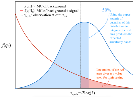
Figure 2.24: Illustration of a test statistic PDF. The $q$ value calculated for the observed data at a given value of $\sigma=\sigma_{\mathrm{test}}$ is $q_{\sigma,\mathrm{obs}}$. Figure modified from [206].

The next step is to “invert” the test above to find a confidence interval using the Neyman construction as illustrated in Figure 2.25. For the observed data, $p\left(\sigma\right)$ was calculated over a range of test hypothesis (top left), and the values of $\sigma$ were rejected when $p\left(\sigma\right)<1-\alpha$ (top right). Combining results for many different masses results in the final limit curve shown in the publications (bottom).

LUX used a constrained extended unbinned two-sided likelihood function. A two-sided confidence interval allows a seamless transition between limits and allowed region since the test hypothesis $\sigma$, and the alternative hypothesis $\hat{\sigma}$ can have either more or less signal strength, unlike a one-sided PLR test which restricts the definition of incompatibility to mean $\hat{\sigma}<\sigma$ [240]. As an example, the likelihood function used for the WS2013 result was

$$\mathscr{L_{\mathrm{WS2013}}\left(\mathcal{D}_{\mathrm{obs}}|\sigma,\theta\right)=} \mathrm{Poiss}\left(n_{\mathrm{obs}}|n_{\mathrm{exp}}\right)$$

$$\times\prod_{e=1}^{n_{\mathrm{obs}}}\frac{1}{n_{\mathrm{exp}}}\left[n_{x}\left(\sigma,k_{\mathrm{Lind.}}\right)f_{x}\left(\mathbf{x}_{e}|g_{2,DD}\right)+\sum_{b}n_{b}f_{b}(\mathbf{x}_{e})\right]$$

$$\times\prod_{e\in\mathrm{constr.}}\mathrm{Gauss}\left(\theta_{i}|\theta_{i}^{\mathrm{exp}},\Delta\theta_{i}\right)$$ (2.20)

where the parameter of interest is $\sigma$, the WIMP-nucleon elastic scattering cross section, and $\theta$ are the nuisance parameters. The number of events each with observables $\mathbf{x}$ in the dataset $\mathcal{D_{\mathrm{obs}}}$ is $n_{\mathrm{obs}}$. In WS2013 the observables were

$$\mathbf{x} =\left\{r,z,S1,\log_{10}S2\right\}$$ (2.21)

where $S1$ and $S2$ are the corrected pulse sizes and $\left(r,z\right)$ describe the reconstructed position of the event. The nuisance parameters $n_{b}$ are for expected counts in each background population, $n_{s}$ is the expected number of signal events and $n_{\mathrm{exp}}=n_{s}+\sum n_{b}$ are the total expected counts and therefore the normalization of the full model PDF. The first term is the Poisson probability of observing $n_{\mathrm{obs}}$ events when expecting $n_{\mathrm{exp}}$, hence “extended” likelihood. The second term represents the weighted sum of background PDFs $f_{b}(\mathbf{x})$ and signal PDF $f_{x}\left(\mathbf{x}_{e}|g_{2,DD}\right)$; this is where the term unbinned comes in as it is a product of the probabilities of each observed event, where the model is the weighted sum of the signal and background component PDFs. The third term enforces Gaussian constraints (hence “constrained”) on a subset of the nuisance parameters $n_{\mathrm{exp}},\,k_{\mathrm{Lind.}},\,g_{2,DD},\,n_{b},\,\theta_{i}$.

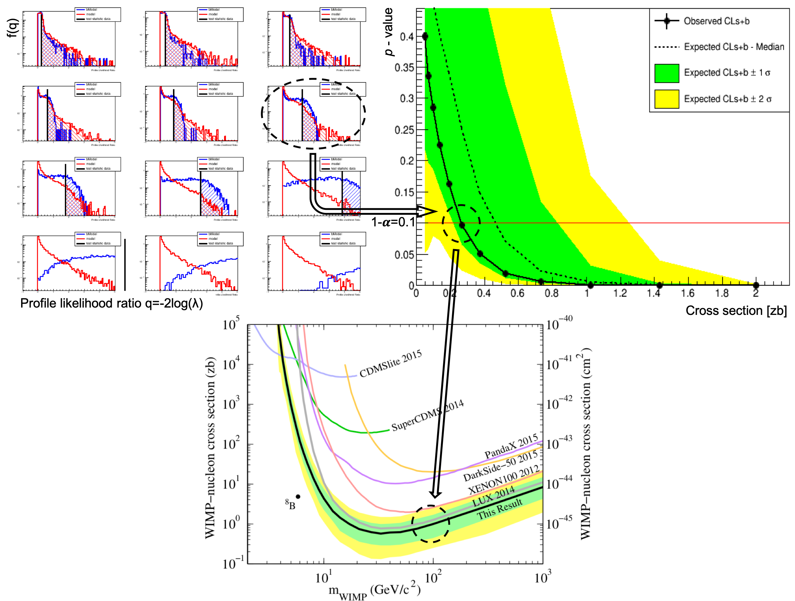
Figure 2.25: Top left: Nine examples of a test statistic PDF for a given WIMP mass and varying cross-sections $\sigma_{\mathrm{test}}$ as constructed by a suite of Monte Carlo pseudo-experiments. Black vertical lines show $q_{\mathrm{obs}}$ determined from data. Each entry in each of the nine plots corresponds to a value of $q$ as calculated from a simulated dataset generated from either given the null hypothesis where $\sigma=\sigma_{\mathrm{test}}$ (red) or an alternative hypothesis $\sigma=0$ (blue). Note the increasing separation as $\sigma$ increases since higher $q$ indicates a greater disagreement between the data and the test hypothesis. i.e., pseudo experiments to the right of the black line indicate the rejection of the signal + background hypothesis. Each plot corresponds to a single black data point in the right-hand plot. Top right: The frequentist hypothesis test inversion to obtain the expected 90% CL is shown for the test points on the left. The $y$ axis corresponds to $p\equiv 1-CL$. Bottom: Upper limits on the spin-independent elastic WIMP-nucleon scattering cross section at 90% confidence limit from [187]. The 1- and 2-$\sigma$ ranges of background-only trials for this combined result are shown in green and yellow, respectively creating the Brazil band. The black arrows track a single point to illustrate the way plots get populated.

Furthermore, the LUX results were “power constrained” [244] to some quantile of the expected distribution in case of a lucky downward fluctuation in the background rate that might result in a confidence interval which is too good, i.e., excluding cross section to which the detector is insensitive for zero backgrounds. Further details regarding both WS2013 and WS2014-16 likelihood functions and the application of the PLR in the LUX analysis was discussed extensively in [206].

2.4.2 WS2013

The initial dark matter search consisted of 85.3 live-days using 118 kg of fiducial mass (out of the 250 kg of active LXe mass) of WIMP search data acquired between April 21 and August 8, 2013. A non-blind analysis was conducted on the WIMP search data, where only a minimal set of data quality cuts, with high acceptance, was employed to reduce the scope for bias. The first, world-leading limit for the LUX detector, obtained using a rapid analysis from Run3 was reported in [101].

Parameter	Value	Unit
Live-time	95	days
Fiducial radius	20	cm
Fiducial drift time	[38, 305]	$\mu$s
Fiducial mass	$145.4\pm 1.3\,\mathrm{}$	kg
Electric field	$180\pm 20\,\mathrm{}$	V/cm
$g_{1}$	$0.117\pm 0.003\,\mathrm{}$	phd
$g_{2}$	$12.1\pm 0.8\,\mathrm{}$	phd
$S1$ threshold	[1, 50]	phd
$S2$ threshold	> 165	phd

Table 2.3: Parameters used in WS2013. The fiducial cut in drift time corresponds to a distance of $\sim 48.6\text{\textendash}8.5\,\mathrm{cm}$ above the faces of the bottom PMTs in $z$. The fiducial mass was calculated by counting tritium events and is consistent with 147 kg expected from geometry. Values of $g_{1}$ and $g_{2}$ were extracted from the Doke plot.

A more careful re-analysis of this dataset increased exposure to 95 live-days of search data, lowered threshold below 3 keV due to the in situ DD NR calibrations, and improved event reconstruction and background model. The improvement in re-analysis of Run3 data resulted in a publication of another world-leading SI limit as described in [187, 186]. This result will be referred to as WS2013. Parameters of WS2013 are summarized in Table 2.3. The cathode and gate grids established the electric field in the active xenon volume. The electric field had a small radial component and thus was not entirely uniform, due to field leakage through the cathode discussed in Chapter 3, an effect that was corrected using the geometric spatial uniformity of ^83mKr. $S1$ pulses were required to have a two-PMT coincidence in the range of 1-50 phd. A lower $S2$ threshold of 165 phd, corresponding to a factor of 6.7 the mean SE response, was applied to mitigate random coincidence background from smaller, isolated $S2$s. ER yields were obtained from ³H calibrations. The in situ DD NR calibrations provided measurements of scintillation yields down to 1.1 keV and ionization yields of 0.7 keV. The resulting efficiency plot is shown in Figure 2.26. The expected neutron background was $0.08\pm 0.01$ NR events in the WIMP search sample.

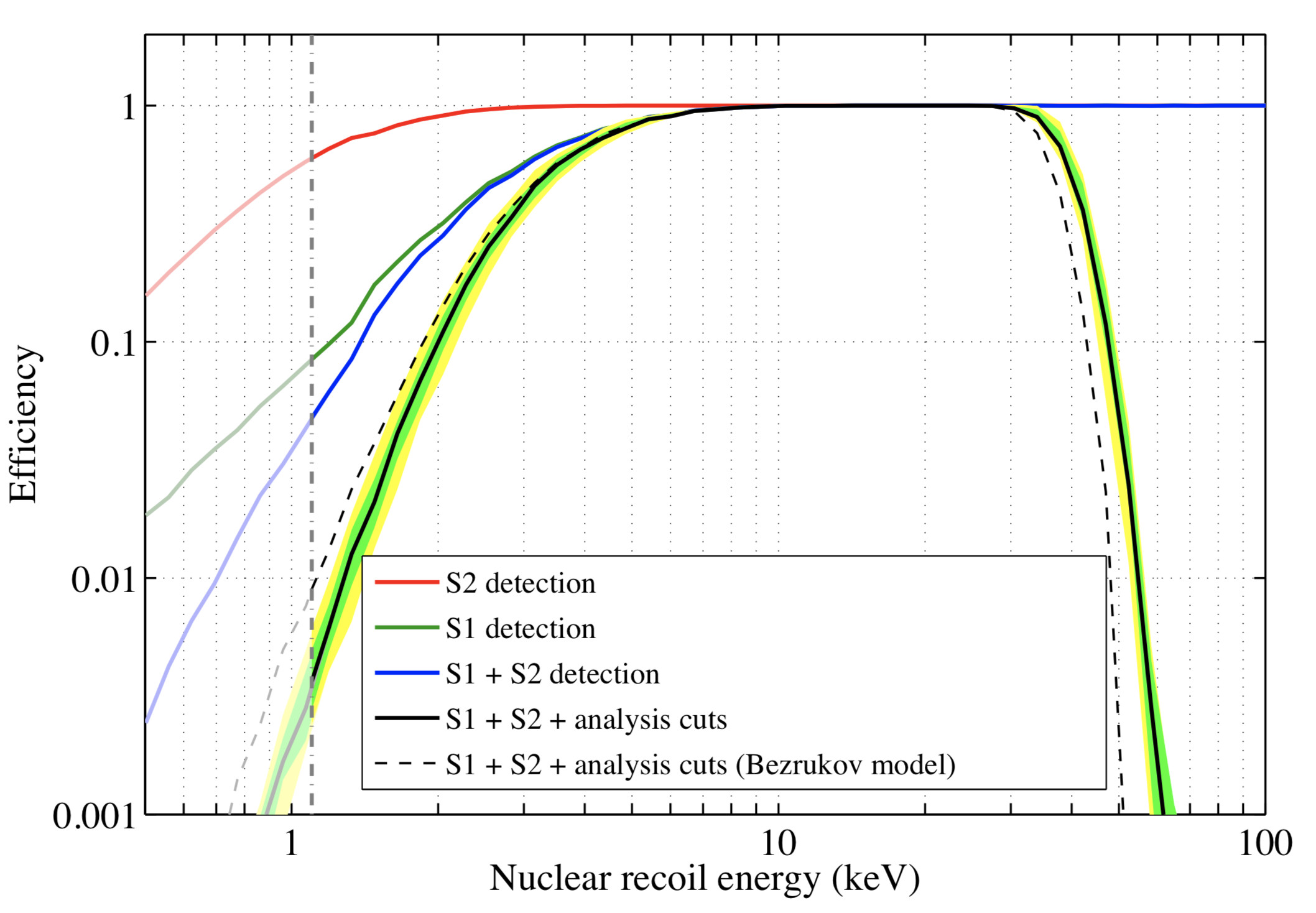
Figure 2.26: Detection efficiency of nuclear recoils in WS2013. The vertical gray dashed line at 1.1 keV indicates the re-analysis threshold. The black solid line shows the best fit of the Lindhard parametrization and the green and yellow shaded regions span the 1- and 2-$\sigma$ uncertainty. Black dashed line indicates an alternative, Bezrukov, NR parametrization. Figure from [193].

Search data analyzed in WS2013 were acquired between April 24-September 1, 2013. Figure 2.27 shows the measured light and charge of the 591 surviving events in the fiducial volume and the upper limit on cross section for WIMP masses from 4-1,000 GeV/c² obtained from the double-sided PLR statistic used to test the signal hypothesis. As is typical for these exclusion limits, at low WIMP masses the signal spectrum falls off at smaller energies and due to lower detector efficiency at these energies, causes the distinguishing upturn of the curve. A decreased flux of WIMPs through the detector causes the characteristic shape of the curve at high masses. Since the total WIMP mass density is fixed at $0.3\,\mathrm{GeV/cm^{3}}$ in the signal model, increasing WIMP mass causes a decrease in number density. Additionally, the highest studied DM mass of 1 TeV/c² is limited by a lack of thorough background simulations at high energies.

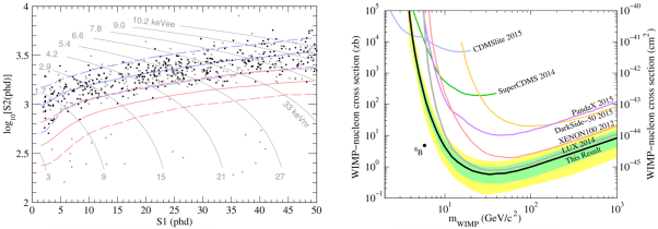
Figure 2.27: Left: The final 591 data points used for WS2013 result. Black data points are at $<18\,\mathrm{cm}$ radius, while points with gray markers are at the edge of the fiducial volume with $r>18\,\mathrm{cm}$. Also shown are the mean (solid) and the 10 and 90% contours (dashed) of the NR (red) and ER (blue) bands for a $50\,\mathrm{GeV/c^{2}}$ WIMP signal. Gray curves show the combined energy scale. Right: Upper limits on the spin-independent elastic WIMP-nucleon scattering cross section at 90% confidence limit. The black curve shows the LUX WS2013 result with expected 1- and 2-$\sigma$ sensitivity bands in green and yellow, respectively. Figures from [187].

Many other results were also obtained using the WS2013 dataset, such as a limit on spin-dependent scattering of WIMPs [245], limits on axions and axion-like particles [246], studies on the effect of pulse shape discrimination in liquid xenon [172], a more general result using effective field theory, and limits on sub-GeV dark matter discussed in Chapter 4. Furthermore, many theses provide descriptions of various LUX components, systems and subsystems, analysis approaches and more for Run3 in great detail in [195, 199, 200, 202, 225, 247, 234, 227, 248, 249].

2.4.3 Grid conditioning campaign

Between WS2013 and WS2014-16, from January to March 2014, the detector grids were conditioned to improve the voltages at which the electrodes could be biased. This was done to increase the magnitude of the applied electric drift field in bulk LXe and to increase the efficiency for extracting electrons from the liquid to the gas. As a result of conditioning, a higher applied anode voltage enabled increased electron extraction efficiency (i.e., the fraction of electrons which promptly cross the liquid-gas interface) from $49\pm 3\%$ in WS2013 to $73\pm 4\%$ in WS2014-16 [163].

During the conditioning, potentials were held just above the onset of sustained discharge and maintained for many days, akin to the burn-in period often employed in room-temperature proportional counter commissioning [250, 251, 252, 253]. First, the potentials on gate and anode grids were raised to -5 kV and 7 kV, respectively, while in cold xenon gas (180 K). Higher glow and electron emission onset points were achieved following this conditioning as shown in Figure 2.28. However, a persistent high POD rate (i.e., the observed PMT pulse) and elevated amounts of PMT noise were observed. This prompted a detector warm up in order to speed up the PMT de-excitation. Subsequently, the potential on the cathode was raised to -20 kV while in xenon gas at room temperature (296 K). The detector was kept at room temperature for one month in April 2014. The detector was then cooled down and filled with LXe again starting on May 6, 2014, enabling the WIMP search data taking to resume in September 2014. Further details about the conditioning campaign can be found in [254].

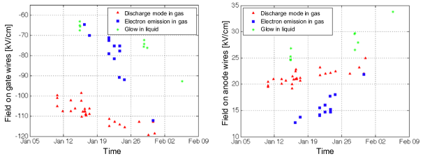
Figure 2.28: Electric fields measured on the gate (left) and anode (right) grid wires throughout the 2014 conditioning campaign. The electric field is plotted at the onset of electron emission in the gaseous xenon (blue square), the onset of discharges in the gas (red triangle), and the onset of glow, or visible photoelectrons on an oscilloscope, while the gate grid is immersed in liquid xenon (green star). Figures modified from [254].

Aside from the increased electron extraction efficiency, the conditioning campaign unfortunately also resulted in some unwanted side effects. In particular, as revealed by $\mathrm{{}^{83m}Kr}$ calibration data, electron drift trajectories were significantly altered compared to the regular near-vertical paths observed in WS2013 due to the electric field variations of 50-600 V/cm. In WS2013, electrons starting from just above the cathode grid at a radius of $r_{S2}\sim 24$ cm traveled slightly radially inwards during their upward drift to the gate due to the field cage geometry alone and exited the liquid surface at $r_{S2}\sim 20$ cm. A similar observation was made in the XENON100 detector [255]. However, in WS2014-16 electrons originating from the same initial radius exhibited a significantly stronger radially inward push and exited the liquid surface at $r_{S2}\sim 10$ cm as illustrated in Figure 2.29. The magnitude of this effect varied in azimuth, depth and furthermore evolved in time, which triggered a need for a full 3D model of the electric fields inside the LUX detector throughout the year-long WS2014-16 data taking. This effort was a crucial foundation for the analysis of the data since knowing the electric field inside the detector is necessary for $(x,y)$ position reconstruction as the drift path of the electrons is field-dependent and for event reconstruction due to the effect of the field on recombination. I developed these field maps; details about this work has been published in [256] and will be discussed extensively in Chapter 3.

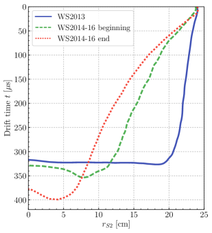
Figure 2.29: Contour plot illustrating detector edges from the reconstructed positions of the $\mathrm{{}^{83m}Kr}$ calibration data. Differences between WS2013 (data from 2013-05-10, solid blue) and the time-dependent WS2014-16 (data from 2014-09-03 with a best fit charge of $-3.6\,\mathrm{\mu C/m^{2}}$, dashed green and 2016-05-03 with a best fit charge of $-5.4\,\mathrm{\mu C/m^{2}}$, dotted red) are seen. Due to the changing electric fields, $\mathrm{{}^{83m}Kr}$ calibration data from the later science run had events with greater drift times.

2.4.4 WS2014-16

Following the conditioning campaign, the first data acquisition of WS2014-16 began on September 11, 2014, and the final data acquisition ended on May 2, 2016. The complications arising from the distorted electric field as a result of the conditioning campaign necessitated many analysis fixes. The WIMP search was interrupted by five ³H and DD calibrations measuring the detector response to ERs and NRs and monitoring the variation of detector conditions. The fiducial volume was defined in the S2 coordinate space with a drift time cut as in WS2013 but a more conservative radial cut including only 101 kg of LXe. An analysis tagging ²¹⁰Pb chain events identified the position of the detector’s PTFE wall in S2 space as described in [235].

Since the light and charge yields in LXe depend on the electric field strength, the large variations of electric field in WS2014-16 caused the ER and NR bands to be substantially smeared throughout the entire exposure, which would cause a reduction of ER-NR discrimination power. Therefore in the analysis, the TPC was not treated as a single homogeneous volume as in WS2013 but instead was segmented into parts within which the field variations were smaller. In particular, the detector was partitioned into 16 segments: four bins of drift time (related to event depth) and four bins of date. Within each segment, the field magnitude was considered to be constant and uniform - the field values are chronicled in [206]. Boundaries in date were September 11, 2014; January 1, 2015; April 1, 2015; October 1, 2015; May 2, 2016 and the boundaries in drift time were 40, 105, 170, 235, 300 μs. The choice of these divisions was driven by the results of the electric field maps and the changing wall position in S2 space and timing of calibration runs. The periodic calibrations of ³H enabled tuning of the empirical NEST ER model for each exposure segment. In practice, this meant varying detector gains as well as Xe response parameters in order to reproduce the observed bands in S1–S2 space. The first and last DD calibrations were performed at multiple heights to define the NR response as a function of different field magnitude at different drift times. The DD campaigns showed minimal variations of the mean and width of the NR band, consistent with the literature [231]. Consequently, the best-fit parameters from the ER calibration data for each exposure unit were applied to the NEST NR model. The fitted models are shown in Figure 2.31.

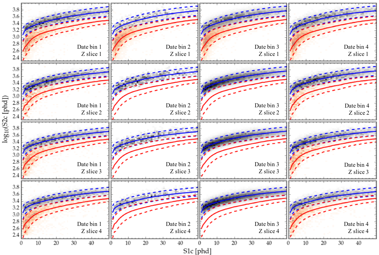
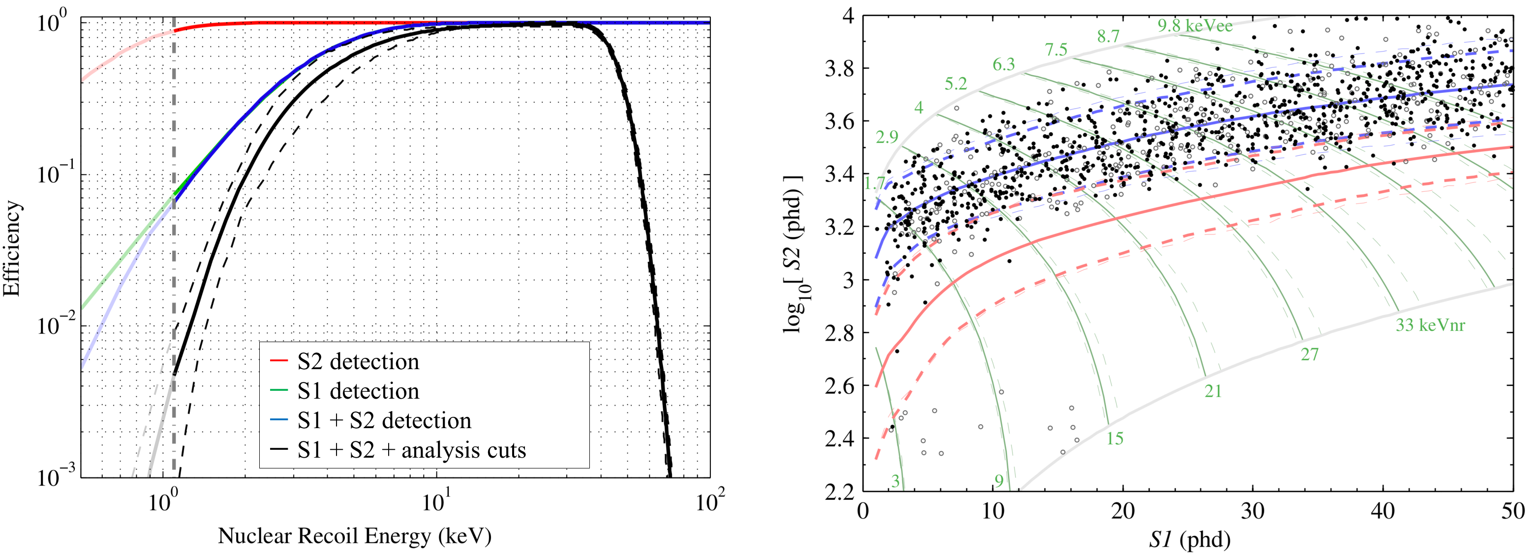
Figure 2.30: ³H (gray) and DD (orange) calibration data. The band medians (solid lines) and 10- and 90% contours (dashed lines) are shown for ER (blue) and NR (red). They were calculated from NEST models of each exposure segment. Note that NEST fitting was performed on ER calibration data only since the resulting parameters from the NR model were found to be in good agreement with the DD calibration data. Only the first and last DD calibrations were performed at various $z$ positions. Figure from [193].

Figure 2.31: Left: The detection efficiencies for nuclear recoils in WS2014-16. The vertical gray dashed line at 1.1 keV indicates the re-analysis threshold. Right: Final 1,221 data points for WS2014-16 passing all selection criteria used for the PLR analysis. Fiducial events within 1 cm of the radial fiducial volume boundary are shown as unfilled gray circles to convey their low WIMP-signal probability relative to the background model. Also shown are the mean (solid) and the 10 and 90% contours (dashed) of the NR (red) and ER (blue) exposure-weighted bands for a $50\,\mathrm{GeV/c^{2}}$ WIMP signal. Green curves indicate the exposure-weighted energy scale. The extrema boundaries from the 16 segments are shown in fainter shade. Figures from [163].

An interpolation of the field map data capable of mapping arbitrary points in real space to S2 space was implemented. This helped to construct the probability models used to test background and signal hypotheses against the WIMP search data. Since the field maps provided a 3D grid of field values, a fast C3PO (Curt’s Post-Processing Position Offset Corrections) interpolation algorithm was used. The background model used in the PLR had three classes of events: events of typical LXe light and charge yield (constructed in a very similar way to WS2013), events affected by proximity to the PTFE wall, and accidental coincidences of isolated S1 and S2 pulses.

In order to minimize any biases, the WS2014-16 dataset was “salted.” Salting is an alternative to the more common approach of blinding where the signal region of interest (i.e., the NR band in our case) is hidden until the entire analysis is finalized. This provides many pitfalls where many unanticipated detector pathologies can remain unnoticed. Salting, also referred to as “spiking,” is common in neutrino experiments, searches for fractional charge, and in gravitational wave detection. LUX used a sequestered tritium calibration dataset to insert $\mathcal{O}\left(100\right)$ events into the data stream. The ³H events were selected to be uniformly distributed in the LXe active volume and their S1 and S2 pulses were patched together to mimic NR signals. Each event was then assigned a random “luxstamp,” a unique event identifier used by LUX, and eventually inserted into the analysis data stream in the event-level file creation stage. A library of salt events was stored in a database with restricted access. Thanks to this approach, LUX analyzers were allowed to use all data generated by the detector. Once the analysis was complete, a person guarding the salt database revealed which of the events that passed all analyses cuts were fake signal events.

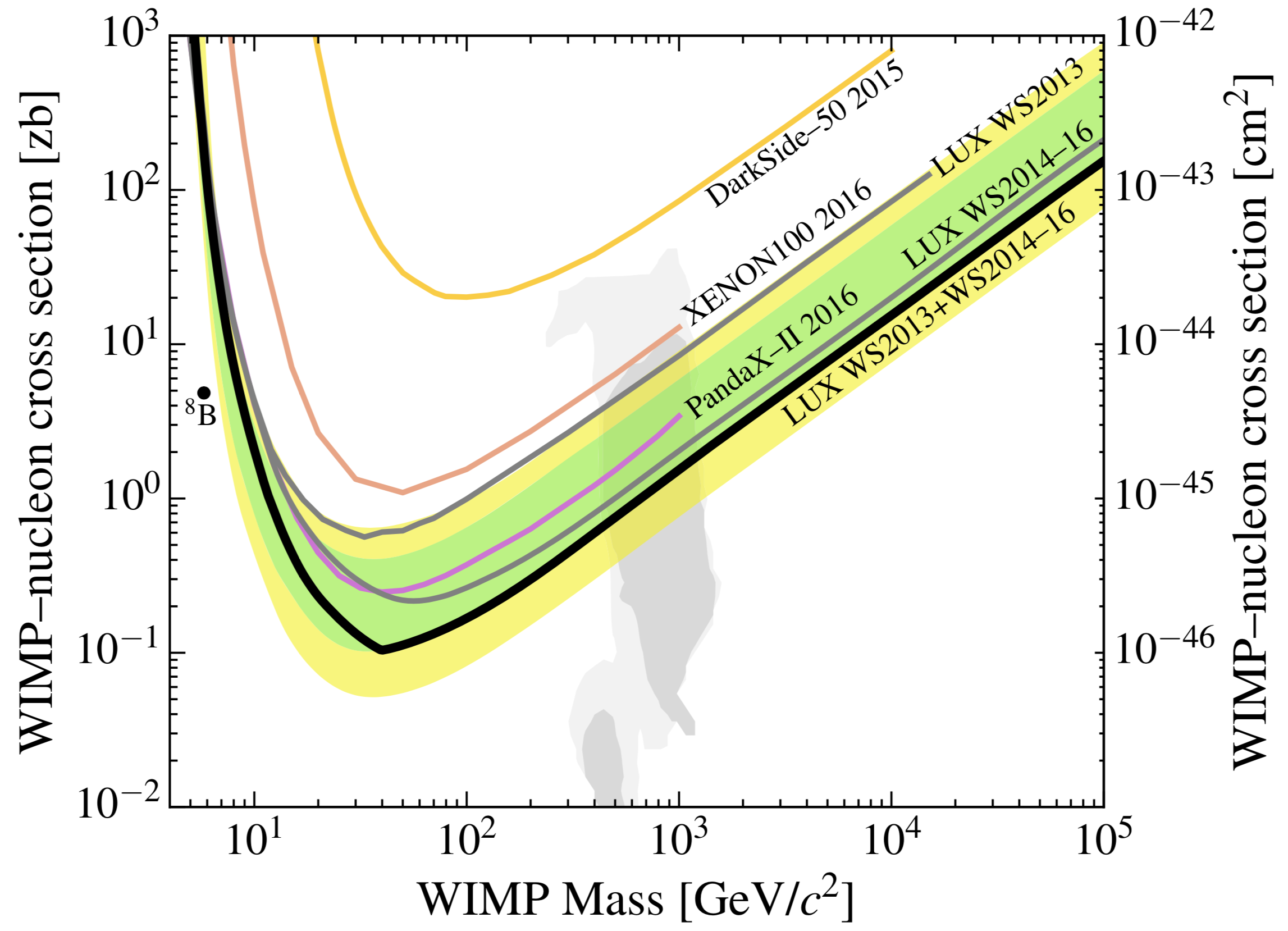
Figure 2.32: Upper limits on the spin-independent elastic WIMP-nucleon cross section at 90% confidence limit. The solid gray curves show the exclusion curves from LUX WS2013 (95 live-days) [187] and LUX 2014-16 (332 live-days). The solid black line shows the limit from these two combined to give the full LUX exclusion curve. The 1- and 2-$\sigma$ ranges of background-only trials for this combined result are shown in green and yellow, respectively. The 1- (light) and 2-$\sigma$ (dark) gray filled regions indicate the parameter space favored by the fully constrained MSSM (CMSSM) [257, 258] before the release of this result. The black ⁸B dot indicates the maximum likelihood of coherent neutrino-nucleus scattering under a WIMP only hypothesis assuming no energy threshold [237]. Figure from [163].

Detection efficiencies for nuclear recoils along with the final dataset with salt events removed are shown in Figure 2.31. In addition to the exclusion limit from WS2014-16 data alone, the exposure from WS2013 was added as a separate 17th exposure segment, which led to another world-leading limit at the time of publication in [163]; the final exclusion limit is shown in Figure 2.32. Limits on the spin-dependent elastic scattering of WIMPs from the complete exposure were also published in [127]. Outside of these publications, many details of the analysis leading to the publication of the aforementioned results have been discussed thoroughly in [193, 206, 224, 235].

2.5 Summary

The immense effort put into its detector design, construction, and operations enabled LUX to collect plentiful data during its operations, which led to many world-leading publications that excluded much of the unexplored WIMP parameter space. LUX also pioneered many calibration techniques now used throughout the field. Furthermore, there are still many ongoing diligent analyses exploring parameter spaces relevant to other dark matter and particle physics models. None of this would have been possible without the tireless effort of all of the collaboration members with whom I had the privilege to work.

Despite its successful operations, LUX still left a significant amount of the WIMP parameter space to be explored by the next generation of dark matter detectors. Looking ahead, both the successful and the less-so successful experiences of LUX are now being leveraged in the design and construction of the LUX-ZEPLIN experiment discussed in Chapter 5.

2.5.1 Contributions to LUX

I joined the LUX collaboration in September 2013, right before the publication of the collaboration’s first world-leading WIMP-nucleon elastic scattering cross section limit. I traveled to SURF in Lead, South Dakota several times as an on-site shifter. My first task underground was to change a diaphragm of one of the two KNF circulation pumps, a very on-topic introduction to the LUX detector, which was rewarded by a box of Chubby Chipmunk chocolates, obviously setting up my time on site to be a success thereafter. I was the Shift Manager and Detector Operations Manager several times. I was trained as an operator of the xenon gas system, liquid nitrogen, PMT, grid high voltage, cathode, DAQ, xenon sampling, external radioactive source deployment, and internal $\mathrm{{}^{83m}Kr}$ calibration systems. I was also trained as an underground guide.

I participated in multiple LUX collaboration meetings and workshops and partook in regular offsite analysis shifts ensuring consistent data quality coming out of the detector. Even though the detector was assembled before I joined the collaboration, I helped on the other end - with the underground detector decommissioning and the detector disassembly and museum prep for the Lead Visitor Center, which allowed me to see the internal detector components that were so carefully modeled in my electric field work.

My most significant contributions to the LUX collaboration were my electric field modeling efforts. This work is discussed in detail in Chapter 3 and in JINST publication [256], where I am the corresponding author. It served as a foundation for many critical analyses that led to the final world-leading SI and SD limits. I also led an analysis searching for sub-GeV dark matter using the novel Bremsstrahlung and Migdal effects. This work is described in Chapter 4 and in [151] that has been accepted to Physical Review Letters for publication, and for which I am the corresponding author.

Chapter 3 3D modeling of electric fields in the LUX detector

Electric fields in the LUX detector changed between WS2013 and WS2014-16. The electric field during WS2013 was nearly uniform in the fiducial volume, but in WS2014-16, the field became quite non-uniform. As discussed in Section 2.4.3, after WS2013 the detector grids underwent conditioning done at very high voltages with intentional continuous glow discharge over many-day periods. This exposed the PTFE walls (that define the radial boundary of the active volume) to VUV photons, which likely caused an in-situ creation of electron-hole pairs in the PTFE surface, thus introducing a new component to the electric fields during the second WIMP search period. The work described in this chapter is published in JINST [256] (WS2014-16) and Phys. Rev. D [186] (WS2013).

This conditioning campaign not only caused a distortion of the detector’s electric field; additionally, the field was observed to be changing throughout WS2014-16 both with time and with azimuthal angle. Since the conditioning altered the electric fields inside the detector in a non-trivial non-symmetric manner, this triggered a need for a fully 3D model of the electric fields inside the LUX detector, varying with date throughout the 23 month-long WS2014-16. Knowledge of the electric fields inside the detector is necessary for $(x,y,z)$ position and event reconstruction since the drift paths of the S2 electrons and recombination are field-dependent.

Mapping of the detector’s electric field was possible due to weekly ${}^{\mathrm{83m}}\mathrm{Kr}$ calibrations with decays uniformly distributed throughout the detector’s active volume. First, a 3D model of the LUX detector was built for WS2013. The fields in the detector were well understood at the time, so this allowed us to cross-check the foundation of the modeling. With the basic model in place, a more thorough and complex model was developed for WS2014-16. To monitor the time-varying behavior in WS2014-16, electric field maps were created on a monthly basis. This was done by fitting a model built in COMSOL Multiphysics to the ${}^{\mathrm{83m}}\mathrm{Kr}$ data, varying the hypothetical charge distributions among 42 spatial subdivisions of the inner PTFE surface and performing fits using an altered Metropolis-Hastings algorithm. The average PTFE charge density was observed to increase in magnitude throughout the exposure, changing from $-3.6\,\mathrm{\mu C/m^{2}}$ to $-5.5\,\mathrm{\mu C/m^{2}}$. The electric field magnitude varied from $\sim 20-50\,\mathrm{V/cm}$ near the bottom of the detector to $\sim 500-650\,\mathrm{V/cm}$, while the mean value of the field of $\sim 200\,\mathrm{V/cm}$ remained mostly constant throughout the exposure.

The electric field in the gas region was modeled to be $\sim 5345\,\mathrm{V/cm}$ in WS2013 and $\sim 6555\,\mathrm{V/cm}$ throughout WS2014-16. This value was assumed to be constant throughout WS2014-16, as charges in the PTFE were shown to not significantly affect this value.

A method describing the development of a 3D electric field model for the LUX detector is outlined in this chapter. However, the method can be applied to model electric fields inside any TPC. We start with an a priori model of the electric fields in LUX based on the engineering CAD designs. This model is then modified to include capabilities of modeling charges in the PTFE walls. The results of the simulations are compared to the ${}^{\mathrm{83m}}\mathrm{Kr}$ calibration data until an agreement is achieved, which enables to map the evolution of electric fields during WS2014-16. This method is then also applied to study field discrepancies seen in WS2013.

3.1 Creating a 3D model of the LUX detector

Electric field models were developed both with and without charge densities in the PTFE panels to understand the detector behavior. Prior to developing a model for the changing electric fields during WS2014-16, a 3D model was developed without static charges in the PTFE panels to confirm our understanding of the calibration data from WS2013. The 3D model was built using the AC/DC Module of COMSOL Multiphysics v5.0® [259], a commercially available finite element simulation software. The lack of symmetries, such as the regular dodecagonal nature of the detector or the parallel grids that were rotated with respect to each other, ruled out the option of using an axially symmetric electric field model as is usually done in this field.

3.1.1 LUX 3D model geometry

The detector 3D model used in the electric field simulations is based on the LUX detector geometry as constructed in LUXSim, the Geant4-based simulation framework used by the collaboration, with CAD drawings used for reference. A full 3D model was needed due to the detector’s geometry. The active volume takes the shape of a regular dodecagonal prism as shown in the left panel of Figure 3.1. Four detector grids (bottom shield, cathode, gate, top shield) are rotated by $60^{\circ}$ with respect to each other (with bottom shield grid and gate being parallel to each other), leaving a geometry that is not azimuthally or otherwise symmetric. The 2D cross-section of the model used in the 3D simulations is shown in the right panel of Figure 3.1; the figure also illustrates some of the adopted simplifications.

Due to the high degree of complexity of the detector, many simplifications were adopted in the model compared to the real-life detector. Since the focus of the modeling was on the active region of the detector, the bottom shield and anode grids were modeled as planes imposing electrostatic boundaries for the top and bottom of the detector. This enabled the model to ignore many details included beyond those grids. The field shaping rings inserted inside a volume of ultra-high-molecular-weight polyethylene (UHMW) were included, but the resistor chain connecting them, and many details of the UHMW structure, as well as the details of the PTFE walls, were omitted. This decreased the computational requirements for solving the 3D model since these only result in very localized effects. The relative DC dielectric constants of the materials used in the model were: $\varepsilon_{\mathrm{liquid\,xenon}}=1.95$, $\varepsilon_{\mathrm{gaseous\,xenon}}=1.0$, $\varepsilon_{\mathrm{PTFE}}=2.1$, $\varepsilon_{\mathrm{UHMW}}=2.3$.

There are three large metal objects inside the UHMW volume of potential concern that were omitted in the LUX COMSOL model: the heat exchanger (ground), the weir (also at ground) and the cathode cable (at -10/-8.5 kV). The detector was designed so that no parts in the UHMW region would affect the electric field inside the detector’s active volume. This was cross-checked by building a second LUX model identical to the one shown in Figure 3.1 but with the heat exchanger, weir and cathode cable included. The simulation confirmed that those parts indeed do not affect the electric field inside the active region; therefore these components were omitted in future models.

Since the model spans five orders of magnitude in length scale (from 28 μm for the grid wire diameter to 1.1 m for the inner vacuum cryostat height), the cathode and gate grid wires were modeled as parallel lines with zero diameter to accelerate the convergence of the model. As with all simplifications, simulations were done that show that this wire diameter change had a negligible effect on the resulting solution without a loss of field resolution (see also calculations done in [260]), especially when using the “Physics mesh” of the COMSOL meshing sequence. Further details about the detector grids along with applied voltages for WS2013 and WS2014-16 are summarized in Table 3.1.

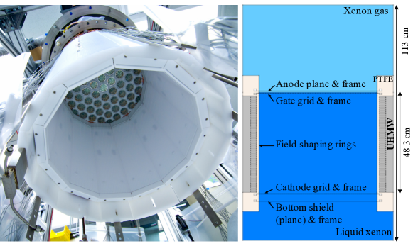
Figure 3.1: Left: Bottom view of the LUX detector showing the regular dodecagonal prism shape, the PTFE panels, and the top PMT array. Right: Cross section of the LUX model including material details. The radius of the inner vacuum can is 30.16 cm while the width of each of 12 innermost PTFE panels is 12.67 cm so that the radius of the inscribed circle (or the separation of parallel panels) is 23.65 cm. The liquid level was assumed to be 3.6 mm above the gate grid in WS2013 and 4.4 mm in WS2014-16.

Grid	$z^{\dagger}$ [cm]	Angle [deg]	Wire $\diameter$ [$\mu$m]	Pitch [mm]	Modeled as	WS2013 [kV]	WS2014-16 [kV]
Top shield	58.6	135	50.8	5.00	Absent	-1.0	-1.0
Anode	54.9	N/A	28.4	0.25	Plane	3.5	7.0
Gate	53.9	15	101.6	5.00	$\diameter 0$ wires	-1.5	1.0
Cathode	5.6	75	206.0	5.00	$\diameter 0$ wires	-10.0	-8.5
Bottom shield	2.0	15	206.0	10.00	Plane	-2.0	-2.0

Table 3.1: Grid properties and voltages as relevant to the construction of the electric field model used in WS2013 and WS2014-16 simulations, including a description of geometric simplifications. ^†The vertical distance from the face of the bottom PMT array, which is defined as $z=0$, accounts for thermal contraction as appropriate.

3.1.2 COMSOL Multiphysics

COMSOL Multiphysics® [259] is a finite element analysis, solver, and simulation software. It is a cross-platform, commercially available, general-purpose software. COMSOL Multiphysics can be used not only for conventional physics-based problems but also allows incorporation of diverse coupled physical phenomena using partial differential equations.

The AC/DC module of COMSOL Multiphysics v5.0, released in 2014, was used in this work. In its electrostatics interface, COMSOL solves the differential equations introduced below. In electrostatics, Faraday’s law is simplified to

$$\nabla\times\mathbf{E}=-\frac{\partial\mathbf{B}}{\partial t}=0$$ (3.1)

where $\mathbf{B}$ is the magnetic field and $\mathbf{E}$ is the electric field

$$\mathbf{E}=-\nabla\phi$$ (3.2)

where $\phi$ is the scalar electric potential. The electrostatics physics interface solves Gauss’ law using the scalar electric potential $\phi$ as the dependent variable:

$$\nabla\cdot\mathbf{D}=\rho$$ (3.3)

where $\rho$ is the total charge and $\mathbf{D}$ is the electric displacement field defined as

$$\mathbf{D}=\varepsilon_{0}\mathbf{E}+\mathbf{P}$$ (3.4)

where $\varepsilon_{0}$ is the permittivity of free space and $\mathbf{P}$ is the macroscopic polarization density. In homogeneous, isotropic, nondispersive, linear materials

$$\mathbf{P} = \varepsilon_{0}\chi_{e}\mathbf{E}$$

where $\chi_{e}$ is the electric susceptibility. Hence in linear materials, the constitutive relation for electric displacement is

$$\mathbf{D}=\varepsilon\left(1+\chi_{e}\right)\mathbf{E}=\varepsilon_{0}\varepsilon_{r}\mathbf{E}=\varepsilon\mathbf{E}$$ (3.5)

where $\varepsilon_{r}$ is the relative permittivity and $\varepsilon$ is a scalar permittivity of the material $\varepsilon=\varepsilon_{0}\varepsilon_{r}$. In a dielectric material, the displacement field satisfies Gauss’s law

$$\nabla\cdot\mathbf{D}=\rho-\rho_{b}=\rho_{f}$$ (3.6)

where $\rho_{b}$ is the bound charge and $\rho_{f}$ is the free charge.

Once the detector geometry, materials, electrical dielectric properties, and voltages were assigned to detector volumes and boundaries, this defined the electrostatic conditions since COMSOL has built-in features to compile these relationships. COMSOL then generated a mesh by discretizing the space into tetrahedra, and a proposed field map was generated. Using an adaptive mesh refinement [261] allowed further improvement of mesh quality while minimizing solution error. This process is illustrated in Figure 3.2.

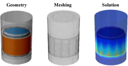
Figure 3.2: Steps in building the 3D model of the electric fields in the LUX detector using COMSOL Multiphysics v5.0. From left to right: First, a geometry was built given materials and their dielectric constants. Next, electrostatic conditions were defined by assigning voltages to conductor boundaries and domains. COMSOL generated a mesh by discretizing the space into tetrahedra and then solved the model. Using COMSOL’s adaptive mesh refinement allowed to improve meshing further while minimizing solution error. The mesh of the LUX model had $\sim 29,000,000$ mesh elements and took about 95 GB of RAM to find a solution. After the model was created, an array of electric field values from the active volume was exported for further analysis.

3.2 Modeling the LUX detector without charges

The electric field in the fiducial volume of the detector during WS2013 was assumed to be uniform in the analysis despite the slight radial field component that pushed S2 electrons toward a smaller radius as discussed below. There was also a small azimuthal contribution near the walls outside of the fiducial volume, discussed in more details in Section 3.4, which did not affect the WS2013 analysis. Overall, the field behavior was well understood and created an opportunity to build, test, and understand the results of the initial 3D COMSOL Multiphysics LUX model.

The electric field values found in COMSOL Multiphysics were exported and used to produce a simulation dataset of electron-like particles in Python v2.7. This was accomplished by starting electron-like test particles uniformly throughout the detector’s active volume and recording their intersection with the liquid surface after drifting. These particles were propagated step-wise in 1 to $3\,\mathrm{\mu s}$ intervals using an interpolated velocity documented in Table 3.2. This was necessary because the electron drift velocity in LXe varies with the electric field, as shown in Figure 3.3. Once the electron-like test particles reached the liquid surface, the simulated drift time $t\mathrm{{}_{sim}}$ and location of the simulated S2 light production ($x_{S2_{sim}}$ , $y_{S2_{sim}}$) were compared with the ($x_{S2}$, $y_{S2}$, $t$) distribution of ${}^{\mathrm{83m}}\mathrm{Kr}$ calibration data.

Figure 3.5 illustrates the 3D nature of both datasets. Excellent agreement was seen as shown in Figure 3.5, without a need to tune any aspect of the model to improve agreement with the data. The 3D data match very well, which is more easily visualized via a 2D summary. Similar to Figure 2.29, the contours were created by finding the average number of events in all the non-empty bins of a 2D histogram in $\left(r_{S2}^{2},t\right)$ and then drawing a contour through those bins that contained half of the average number of events. Therefore the contours approximate the edges of the detector’s active volume. The mean value of the electric field inside the fiducial volume during WS2013 was $177\pm 14\,\mathrm{V/cm}$ as calculated from the COMSOL Multiphysics simulation.

Electric field [V/cm]	20	38	51.8	68	105	182	375	727	1000
Velocity [mm/$\mu$s]	0.55	0.89	1.05	1.19	1.39	1.53	1.72	1.86	2.00

Table 3.2: Electron velocity in LXe used in simulations [262, 263, 264].

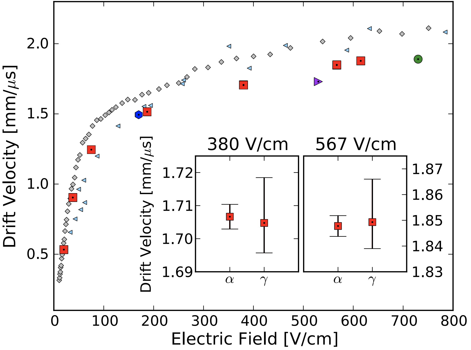
Figure 3.3: Electron drift velocity in LXe measured by the EXO-200 collaboration (167 K, red square). Also shown are results from Miller et al. (163 K, cyan triangle) [265], Gushchin et al. (165 K, gray diamond) [266], XENON10 (177 K, green circles) [264], XENON100 (182 K, purple triangle) [267], and LUX (175 K, blue hexagon) [101]. Values used in this work are listed in Table 3.2. Figure from [262].

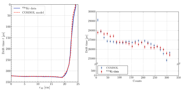
Figure 3.4: Scatter plot illustrating the 3D nature of the simulation.

Figure 3.5: Left: Contour plot showing histogram edges of the 3D field model and ${}^{\mathrm{83m}}\mathrm{Kr}$ events averaged over all azimuthal angles during WS2013. Data (solid blue) and simulation (dashed red) contours agree without any fitting or tuning necessary. Right: The distribution of events at varying $z$ position agrees between the ${}^{\mathrm{83m}}\mathrm{Kr}$ data and the simulation.

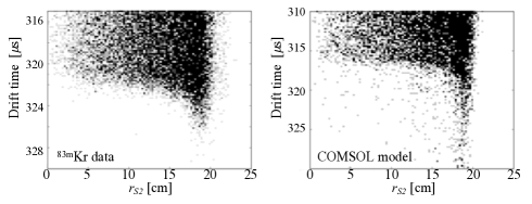
Figure 3.6: Results from an axially symmetric COMSOL Multiphysics model (for illustration purposes.) Left: Electric field lines and equipotentials in the LUX detector during WS2013. Center: Regions in the corners of the detector show field leakage. A low-field pocket at the high radius and low $z$ causes electrons originating in this area to drift inward. This low-field pocket is predominantly due to leakage of the much higher field in the reverse field region (region between bottom shield grid and cathode), as well as the ground voltage of the inner vacuum can. Right: This leakage effect can be mitigated by replacing the cathode grid with a plane with an equivalent potential.

Figure 3.7: Scatter plot of drift time vs. S2 radius for WS2013 ${}^{\mathrm{83m}}\mathrm{Kr}$ data (left) and COMSOL model (right) zoomed in to the low-field pocket showing the extended drift time in the region. The slight quantitative discrepancy is likely caused by a combination of an error on the simulated electron velocity and slightly different dimensions of the real and modeled detector.

The slight curve seen at a high radius and drift time in the reconstructed S2 coordinates can be understood by looking at Figure 3.7. This figure shows equipotentials and field lines from an axially symmetric COMSOL Multiphysics LUX model built for visualization purposes. A ${}^{\mathrm{83m}}\mathrm{Kr}$ event decaying in the bottom right-hand corner of the active volume will follow the field lines shown and end up at a slightly smaller radius than where it started. This slight curvature has been seen before, for example in simulations of the XENON100 experiment [255]. The inward push is due to a low-field pocket seen at the high drift time, high radius corner, which is created by the reverse field region electric field (region between the bottom shield grid and the cathode grid) and the ground voltage of the inner vacuum can leaking through the cathode grid. This low-field pocket goes away when the cathode grid wires are replaced by a solid plane held at the same cathode voltage also shown in Figure 3.7. The low-field pocket creates a mild concern for analysis: the electron-ion recombination varies with field strength much more strongly at low field. As a result, if the field is low enough, then high recombination could potentially create a nearly S2-free detector response, and thus a dead volume unaccounted for in the fiducial volume calculation. However, events in this low-field pocket can be flagged in the data using their long drift times, as shown in Figure 3.7.

A similar field effect is seen near the top of the detector. The high-field pocket causes a region of slightly enhanced $S2/S1$ ratio since high electric field boosts S2 and suppresses S1 signals. Additionally, events occurring at high radius experience a slight inward push. This helps identify PTFE surface events since the radial position resolution is improved by spreading the light over multiple PMTs. Without this inward push, S2 signals of surface events would be primarily concentrated on a single PMT.

3.3 Modeling charges in the LUX detector

After the conditioning campaign that took place between WS2013 and WS2014-16 as described in Section 2.4.3, a substantial change in the detector’s electric field occurred, which affected electron paths as shown in Figure 2.29. This change in the field can be modeled with negative charge densities present in the PTFE panels; the consequence of this accumulated charge is illustrated in Figure 3.8.

The conditioning campaign was performed in xenon gas and exposed the PTFE wall to VUV photons, which created electron-hole pairs within the PTFE surface that defines the radial boundary of the active volume and serves as a reflector to VUV scintillation photons. The subsequent observed time evolution of the PTFE charge is due to the higher mobility of positive charges (holes) relative to the negative charges (electrons), allowing the gradual removal of holes under the applied field and leaving an on-balance negatively-charged surface. This behavior is consistent with a non-uniform time-varying negative charge density in the PTFE panels as described below. Due to PTFE being an excellent insulator, it is very hard to get rid of those charges during the operational lifetime of the detector and therefore it is critical to understand their effects on the electric field. So in an (unfortunate) way, LUX can also serve as a very sensitive static charge measuring device.

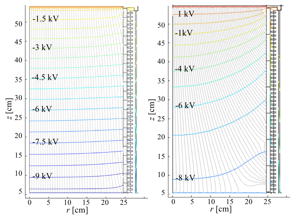
Figure 3.8: Two axially symmetric COMSOL Multiphysics models built for visualization purposes. Left: Electric field lines and equipotentials in the LUX detector during WS2013. A small radially-inward component is seen, resulting from the geometry of the field cage and the grids. Right: Electric field lines implied by ${}^{\mathrm{83m}}\mathrm{Kr}$ from 2015-04-26 showing the much stronger radially-inward component modeled by negative charge densities in the PTFE panels.

To gain intuition about the effects of charge in the PTFE panels on electron paths, a simulation was performed by depositing $-1\,\nicefrac{\mathrm{\mu C}}{\mathrm{m^{2}}}$ of charge density in either the lower, middle, or upper third of a PTFE panel; the resulting force causes inward displacement of electron clouds that originate near or below the charged site, as demonstrated in Figure 3.9.

Figure 3.9: Effect of negative charge densities in the PTFE panels on events in the detector as simulated in the 3D COMSOL model. The four figures illustrate COMSOL models with no charge in the PTFE panels and with $-1\,\nicefrac{\mathrm{\mu C}}{\mathrm{m^{2}}}$ deposited at the lower, middle, and upper segments of a PTFE panel causing a strong inward push for events that originate near or below the charge site.

3.3.1 Alternative explanations for the field distortion

Other than the charge evolution in the PTFE surface, there are other plausible explanations for distorted fields inside a TPC. One possibility would be that drifting electrons land on the PTFE surface and do not get pulled toward the surface due to the high resistivity of PTFE. This is unlikely since the detector is designed to pull electrons up and away from the PTFE surface and because any negative charging will prevent further charge from drifting toward the surface. Other explanations might be a short or open circuit in the field-shaping ring resistor chain. The field distortion caused by a shorted resistor was simulated in the axially symmetric COMSOL model as shown in Figure 3.10. A shorted resistor produces a small, very localized field deformity, unlike the detector-wide field distortion observed in WS2014-16. This effect would also not evolve throughout the detector operation.

An open circuit was simulated in the axially symmetric COMSOL model also shown in Figure 3.10. A field distortion is distinct and not dissimilar to the field observed in WS2014-16. However, depending on the location of the open circuit, it can create large, dead, field-less regions in the detector. The resistance of the field-shaping ring resistor chain was measured before WS2013 and then again before WS2014-16. No significant change was observed, ruling out this explanation. The possibility of an open circuit effect is also ruled out because it would not create a time-dependent component. Additionally, ¹³⁷Cs calibrations [202] were performed in WS2014-16 using the acrylic radioactive-source deployment tubes suspended along the side of the detector, which showed events along the entire detector height, inconsistent with the presence of field-less regions.

Therefore, the LUX collaboration concluded that charges in the PTFE surfaces were the culprit for the varying electric fields. We next describe the electrostatic properties of PTFE generally, before moving to the central work of modeling these charges.

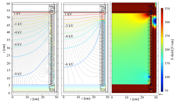
Figure 3.10: Left: Electric field lines as modeled using ${}^{\mathrm{83m}}\mathrm{Kr}$ from 2015-07-22. Center: Electric field lines caused by an open circuit in the field shaping rings. In this case, the connection between the 4^th and the 5^th top ring is broken. A field distortion is obvious and not dissimilar to the field observed in WS2014-16, however, this effect is not only ruled out by our measurement of the resistance of the field-shaping ring chain but would also not be time-dependent. Right: Electric field due to a shorted field ring. In this case, the 5^th field ring from the bottom is shorted. The effect on the field is very localized and does not distort the field nearly as much as what is observed in WS2014-16. All three images come from an axially symmetric COMSOL Multiphysics WS2014-16 model built for illustration purposes only.

3.3.2 Charges in PTFE

Since the goal of this work was to model charges in the PTFE surface, this section offers a brief overview of PTFE properties and their relevance to this analysis.

PTFE is a type of synthetic fluoropolymer of tetrafluoroethylene also known as Teflon™ [268] discovered by DuPont Co. in 1938^,. PTFE is a non-reactive, hydrophobic material with a very low coefficient of friction, high dielectric constant, and good reflectivity for xenon scintillation light. This makes it a very popular material in two-phase dark matter detectors. However, fluorine is the most electronegative element in the periodic table making it a very attractive site for electrons.

PTFE is known as an excellent insulator. Due to its excellent charge storage capacity, it is very popular as an electret in many applications, such as in microphones. Hence many studies have been done investigating PTFE properties at room and elevated temperature, but unfortunately not at the LXe temperatures of 175 K. Resistivity of PTFE has been measured to be $\rho\sim 3\times 10^{20}\,\mathrm{\Omega\cdot cm}$ at $5\times 10^{-6}\,\mathrm{torr}$ at 25^∘C [270]. Charge lifetimes at room temperature have been measured to be $10^{3}-2.6\times 10^{5}$ years [271], which is much longer than what can be inferred from the published PTFE conductivities illustrated in Figure 3.11, a discrepancy that remains an open question, but does not affect results presented in this work.

The PTFE surface has been demonstrated to hold charges of at least $0.1\,\mathrm{mC/m^{2}}$ [272], an order of magnitude more than what was modeled to be observed in LUX. Peak space charge densities of $2500\,\mathrm{C/m^{3}}$ have been reported in corona-charged PTFE with bulk charge densities being 1-2 orders of magnitude smaller [271]. This puts the results presented in this chapter within reasonable bounds.

The grid conditioning done in March 2014 was performed in cold xenon gas. The far ultraviolet emission spectrum of xenon contains five emission lines in the range $117-147$ nm [273] corresponding to energies of $10.6-8.4$ eV. The photoemission threshold energy of PTFE is 10.6 eV while the VUV absorption spectrum shows an intense peak at 7.7 eV likely corresponding to an excitation from the top of the valence band to the bottom of the conduction band [274]. Therefore, discharges during the conditioning campaign had sufficient energy to liberate electron-hole pairs in PTFE. Studies using multiple-needle-plane corona discharges on a PTFE block show that charge created this way mainly exists in the surface layer at $1-2\,\mathrm{\mu m}$.

It has been shown that under an applied field, hole states exhibit significantly higher mobility than electron states. The applied field will gradually transport holes, and the surface charge will become increasingly negative, asymptoting with the hole transport timescale. One study found that after charging the PTFE block for 30 mins by applying a voltage of $\pm 5\,\mathrm{kV}$ at room temperature, the half-life period of surface potential decay was 5 min for hole traps and 150 min for electron traps, reflecting this distinct difference in the surface layer of PTFE as shown Figure 3.11. The energy levels of electron traps and hole traps were about $0.85-1.0$ eV and $0.80-0.90$ eV, respectively [276]. A timescale of hole transport in the LUX PTFE surface as seen in the high purity, low-temperature LXe environment is shown in Figure 3.23.

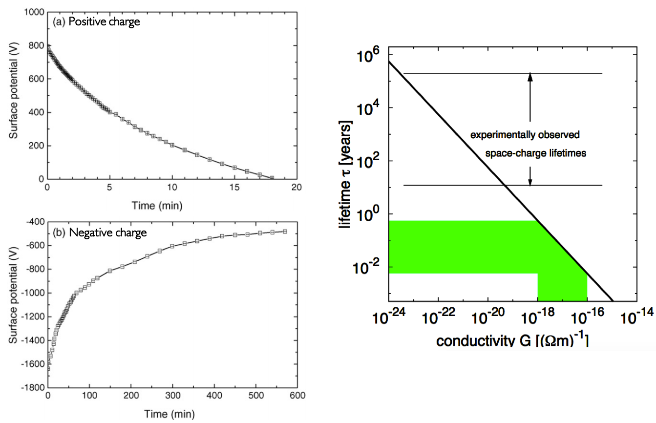
Figure 3.11: Left: The decay curve of the surface potential of PTFE samples while charging positively (top) and negatively (bottom). Figure from [276]. Right: Space-charge lifetime $\tau$ versus electrical conductivity $G$, as given by Equation 3.11. With experimental conductivities between $10^{-16}-10^{-18}\,\mathrm{\left(\Omega\cdot m\right)^{-1}}$ (green shaded area), space charge should decay on a timescale of days or months, rather than millennia. Figure from [271].

In other research areas, PTFE is usually charged up using an electrode contact, which injects electrons across the PTFE surface. A change in conductivity is observed when electrons reach a grounded electrode. This is called the transit time and has been computed for LUX in this work. Another method of charging PTFE is by using a high energy electron beam, which deposits electrons from tens of nm to tens of $\mu$m deep into the surface depending on the beam energy. To mitigate the amount of positive/negative charges in PTFE, the material can be heated up while either blasting an electron gun or shining a VUV light until an equilibrium is reached. Heating the material helps the charge mitigation since both the charge lifetime $\tau$ and conductivity $G$ are temperature dependent [276, 271]:

$$\tau=\tau_{0}\exp\left(\frac{E_{trap}}{kT}\right)$$ (3.7)

where $E_{trap}$ is the trap depth, $T$ is the temperature, $k$ is the Boltzmann constant and $\tau_{0}^{-1}$ set by molecular vibration frequencies ($10^{13}\,\mathrm{Hz}$).

To calculate the transit time, derivation from [271] can be followed. For the case of ohmic conductivity, current density $j$ is given by

$$j=-\frac{d\sigma}{dt}=GE$$ (3.8)

where $\sigma$ is the surface charge density, $G$ is the conductivity and $E$ is the internal electric field. Assuming a thin space-charge layer, the electric field in the sample is nearly homogeneous and given by

$$E=\frac{\sigma}{\varepsilon_{0}\varepsilon_{r}}$$ (3.9)

where $\varepsilon_{r}=2.1$ for PTFE. Solving the differential equation obtained by inserting Equation 3.9 into Equation 3.8 yields an equation for the time decay of surface charge

$$\sigma=\sigma_{0}\exp\left(\nicefrac{{-t}}{{\tau}}\right)$$ (3.10)

where $\sigma_{0}$ is the initial surface charge, and charge lifetime $\tau$ is given by

$$\tau=\frac{\varepsilon_{0}\varepsilon_{r}}{G}.$$ (3.11)

This result will be used in Section 3.3.4.1 to estimate the average charge density in LUX throughout WS2014-16.

3.3.3 Modeling changing electric fields in WS2014-16

The effect of the inward push from the electric field is apparent from an event from WS2014-16 shown in Figure 3.12. Here an event that originated near the bottom of the detector was pushed inward while drifting. This phenomenon causes problems in analysis, not only for the field-dependent recombination but also for position reconstruction, since an electron cloud that starts near the center and top of the detector has the same $\left(x,y\right)$ position as a cloud that starts near the edge but at the bottom of the detector.

This effect was corrected in the analysis using field maps, the output of this work. This section provides a detailed description of the approach adopted to model the electric fields throughout WS2014-16 and resulting in those field maps. A summary of the contents of this section is illustrated in Figure 3.13.

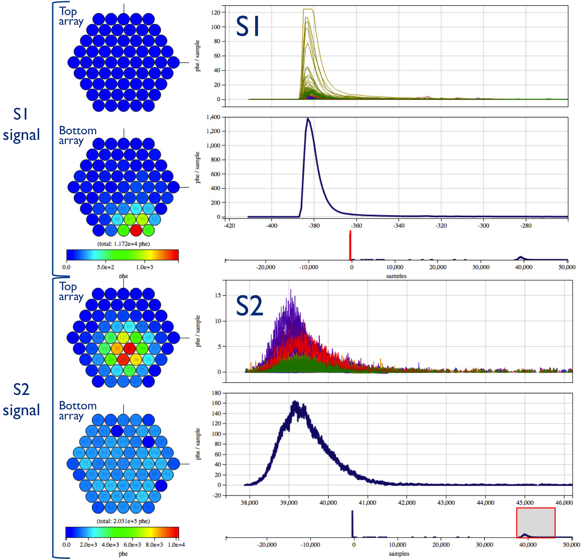
Figure 3.12: A detector event showing the strong field effect due to wall charges from July 23, 2015, during WS2014-16. The top image shows an S1 pulse near the detector wall above the cathode at $390\,\mathrm{\mu s}$, while the bottom image shows the successive S2 pulse as it reaches the liquid surface. The four plots on the right show the waveforms as seen by each PMT (multiple rainbow colored lines) and the summed average across the top and bottom PMT arrays (wide blue line) for both the S1 and the S2 signal. The timeline is given in samples (1 sample = 10 ns). The schematics on the left shows the amount of light seen by each PMT at the top and bottom arrays. From the location of light seen by the PMT arrays, the event migration toward the center of the detector on its way up can be observed. Images are taken from Visualux, the LUX dataset preview software 3.12.

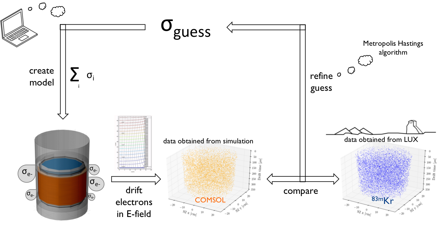
Figure 3.13: Illustration of steps involved in modeling electric fields during WS2014-16. First, a model of the LUX detector with 42 tiles was created in COMSOL. The use of superposition principle then enabled placement of any combination of charges $\Sigma_{i}\sigma_{i}$ on detector walls (bottom left). Simulated particles were then drifted through that charge distribution. The simulated particles (orange scatter plot) were compared with real data from the detector (blue scatter plot) and using the Metropolis-Hastings algorithm a more accurate guess $\sigma_{\mathrm{guess}}$ was generated. This process was iterated until convergence between simulation and data was observed.

3.3.3.1 Principle of superposition

To model the detector behavior in WS2014-16, first, the charge-free model described in Section 3.2 was modified to include WS2014-16 grid voltages. Then 42 additional COMSOL Multiphysics models were built, with voltages on all boundaries set to 0 V. The 12 PTFE panels surrounding the active volume were split into 42 tiles by defining 6 angular and 7 vertical divisions of equal width and height. Therefore there were 2 PTFE panels in each angular division. Each one of the 42 models included $-1\,\mathrm{\mu C/m^{2}}$ of charge on one of the 42 tiles. These 43 datasets (arising from 42 models with charge and one without charge) served as basis vectors since the charge on any tile could be scaled up or down as needed. Note that this linear superposition of basis charges is valid since the electric field arising from two isolated charges is equal to the sum of the electric fields arising from each charge individually. Leveraging the superposition principle, these models could be linearly combined to produce electric field maps based on arbitrary charge distribution. Those models were solved in COMSOL Multiphysics. The resulting 43 electric field vector maps were exported on a $1\,\mathrm{cm^{3}}$ grid to a Python environment where all further calculations were performed.

Each one of the 42 tile models could be multiplied by a different charge density to create any charge configuration desired as seen in Figure 3.14. All further calculations were done in a Python environment to allow for easier and faster superposing.

The choice of the number of tiles used was optimized to balance two opposing effects: more tiles result in a better real-life approximation, but it also increases computational requirements due to the high number of free parameters for minimization. To test this method, a simpler model was initially created in which the PTFE panels were split only into 15 tiles: 3 angular and 5 vertical divisions. However, the granularity of the model was too large, which led to the development of a model with a higher number of tiles. A model with a finer granularity was not tested since even the 42-basis vector model used in the analysis was quite complex given the available resources and time constraints, and required manual adjustments to converge within the necessary time window.

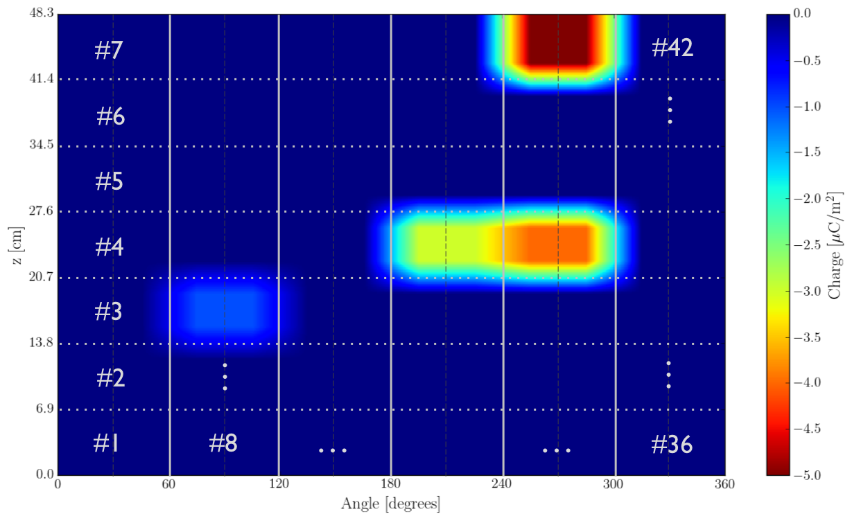
Figure 3.14: Illustration of the PTFE wall with split into 42 tiles, where each tile can contain a different amount of charge density. The smoothing function described in Section 3.3.3.2 avoids unphysical sharp drops between neighboring tiles with different charge densities.

3.3.3.2 Smoothing function

Unphysical behavior emerged when two neighboring tiles that constitute the 42 basis vectors contained very different charges. To mitigate these sharp discontinuities, the charge on each tile was set to fall off linearly both in the azimuthal and in $z$ directions. This smoothing was defined such that in the azimuthal direction each tile had a uniform $-1\,\mathrm{\mu C/m^{2}}$ charge density from $\nicefrac{{1}}{{4}}$ to $\nicefrac{{3}}{{4}}$ of tile width. This charge density then decreased linearly to $0\,\mathrm{\mu C/m^{2}}$ through $\nicefrac{{1}}{{4}}$ of the width of the neighboring tile. Therefore the charge density in the azimuthal direction was continuous. The same technique was applied in the $z$-direction except that the bottommost and topmost edge tiles were smoothed in only the direction pointing toward the center of the panel.

3.3.3.3 Metropolis-Hastings algorithm

With the charge density basis vectors defined, an iterative process was used to find the true charge in the PTFE panels. First, a hypothesized charge distribution was defined, and each one of the 42 charge basis vectors was multiplied accordingly. The electric fields from each basis vector simulation were combined to produce a hypothetical electric field inside LUX. Simulated particles were drifted through this electric field, and a likelihood function was used to compare the outcome to ${}^{\mathrm{83m}}\mathrm{Kr}$ data. Then the initial charge hypothesis was refined, and this approach was iterated using the Metropolis-Hastings algorithm until convergence of results was observed.

The Metropolis-Hastings algorithm is a Markov Chain Monte Carlo method for sampling from a multi-dimensional distribution with a high number of degrees of freedom. First, an initial guess was made for the amount of charge on each tile, and the corresponding model was created. Each subsequent guess was randomly sampled from a Gaussian distribution centered at each charge density with a width of $\sim 0.1\,\mathrm{\mu C/m^{2}}$. The ideal step size was tuned to achieve acceptance of new charge distributions of $\sim 23\%$ [277], where the acceptance ratio was defined as

$$\alpha=\frac{\mathcal{L_{\mathrm{new}}}}{\mathcal{L}_{\mathrm{old}}}.$$ (3.12)

Here, $\mathcal{L_{\mathrm{new}}}$ and $\mathcal{L}_{\mathrm{old}}$ are the log likelihood functions for the current and previous steps, respectively.

To speed up the convergence at the beginning of the modeling efforts, the amount of charge in the PTFE panels was adjusted manually to smooth out charge deviations between neighboring vertical panels before using the Metropolis-Hastings algorithm. As the dataset neared convergence, a modified Metropolis-Hastings algorithm was used due to the high number of degrees of freedom (42). Instead of varying all charges simultaneously, as is usual for the algorithm, only one random charge was varied at a time, which sped up convergence.

3.3.3.4 Modeling detector observables

To model the electric field, the simulation results were compared to the field implied by ${}^{\mathrm{83m}}\mathrm{Kr}$ calibration data to ensure its accuracy, since the real value of the electric fields inside of the detector was unknown. An initial (but unsuccessful) attempt to solve this problem involved drifting electron-like particles, similar to the approach outlined in Section 3.2. However, $\sim 100,000$ particles were needed (corresponding to particles spaced $1\,\mathrm{cm^{3}}$ apart) to capture enough details of the active volume, which was too computationally slow. This comparison had to be done many times during the Metropolis-Hastings algorithm, rendering the traditional method of drifting electrons through the detector computationally too intensive, so an alternative method comparing event densities was developed. The comparison was made first throughout the entire detector active volume and at the final stages of refinement only by comparing the edges of the distributions.

Instead, ${}^{\mathrm{83m}}\mathrm{Kr}$ events as seen in S2 space were reverse-propagated through the modeled drift field to find the initial homogeneous distribution. In practice, this was accomplished by segmenting the ${}^{\mathrm{83m}}\mathrm{Kr}$ data into tetrahedra within the active volume using Delaunay triangulation [278] and recording the number of events enclosed by each segment. The vertices of those tetrahedra were drifted “back in time” through the electric field; each vertex started at the liquid surface and was drifted through the active volume, transforming S2 space to real space. The new volume of each tetrahedron after drifting, $V_{tet}$, was calculated and the number of ${}^{\mathrm{83m}}\mathrm{Kr}$ events, $n_{S2}$, contained in each tetrahedron recorded. Since in real space ${}^{\mathrm{83m}}\mathrm{Kr}$ events were uniformly distributed throughout the detector, the number of events in each tetrahedron was proportional to its volume

$$n_{real} = N_{Kr}*\frac{V_{tet}}{V_{TPC}}$$ (3.13)

where $N_{Kr}$ is the total number of ${}^{\mathrm{83m}}\mathrm{Kr}$ events in the detector and $V_{TPC}$ is the active volume of the detector. If the simulated electric field captured the field in the detector well, then $n_{real}$ and $n_{S2}$ had an equal number of events. A $\chi^{2}$ was then calculated to compare data to simulation, and the charge guess refined. This approach was iterated until convergence of results was seen. The density comparison between ${}^{\mathrm{83m}}\mathrm{Kr}$ data and simulation is illustrated in the right panel of Figure 3.17.

3.3.3.5 Comparing edges

To complete the fine-tuning of the model, the edges of the ${}^{\mathrm{83m}}\mathrm{Kr}$ distribution were compared with data, in a method independent of the ${}^{\mathrm{83m}}\mathrm{Kr}$ homogeneity in the detector. The detector was split into 12 angular sections corresponding to the 12 PTFE panels. Then negative charges were drifted to the liquid surface starting along the center of each panel face. An offset radius (set at $r$ = 22 cm) was used due to a higher fidelity of field maps slightly inward from the PTFE panels. The resulting simulated edge at the detector wall ($r$ = 23.7 cm) agrees with the edge found both from the ${}^{\mathrm{83m}}\mathrm{Kr}$ data as shown in Figure 3.15 and from the location of the wall as determined from ²¹⁰Po background [279] (shown in Figure 3.16). It is worth noting that even though only the detector wall was fitted, as shown in the left panel of Figure 3.17, the result correctly described the density distribution inside the entire detector.

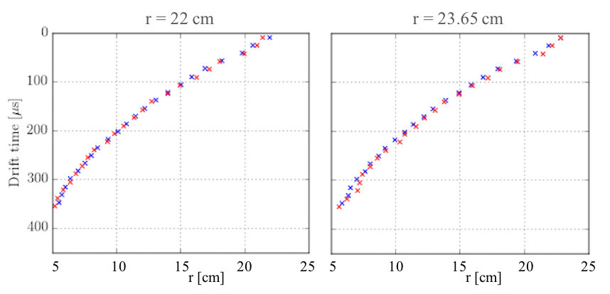
Figure 3.15: Comparison of wall position as found using ${}^{\mathrm{83m}}\mathrm{Kr}$ data (blue) and COMSOL model (red) at two different radii. Radius $r=23.65\,\mathrm{cm}$ corresponds to the detector PTFE wall. Data shown is from 2015-07-22 in $-15^{\circ}<\theta\leq 15^{\circ}$ azimuthal section of the detector.

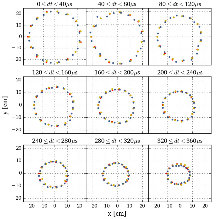
Figure 3.16: Wall position as found using three different methods for the period of 2014-12-07 to 2015-03-19. Wall positions as found from the wall model using ²¹⁰Po (blue) [235], 95% of ${}^{\mathrm{83m}}\mathrm{Kr}$ from 2015-01-22 (red) and 95% edge of the field map for 2015-01-22 (yellow); all three models agree.

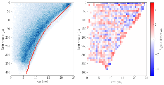
Figure 3.17: Left: Solid red contour at $r$ = 22 cm illustrates the modeled edge of the ${}^{\mathrm{83m}}\mathrm{Kr}$ distribution (blue) from 2016-02-22. Right: variation between normalized histograms of ${}^{\mathrm{83m}}\mathrm{Kr}$ data and simulation from 2016-10-06 weighted by the error in each bin (using an azimuthal slice between $120^{\circ}\leq\theta<180^{\circ}$).

3.3.3.6 Validation

Before developing the simulation with 42 charge segments, a test model was created using 3 angular and 5 $z$ slices resulting in 15 charge segments. As an initial test, a dataset was simulated with known charge distribution at the 15 sites. Then, starting with random charge distributions on the 15 tiles, the simulation successfully converged to the expected values.

The model with 42 charge segments was first tested by making sure the charge distribution successfully converged to a test dataset that included no charges on the PTFE walls. However, in order to converge to a model with a known charge distribution, the model with 42 free parameters required much more computational power than the 15 parameter model. As a result, the 42-tile model never reached a high enough confidence in the algorithm convergence alone (as it would have taken perhaps years to converge). In order to deliver results to the LUX collaboration in a timely manner, the state of the algorithm was visually inspected throughout the fitting procedure to make sure that the best-fit charge distribution matched ${}^{\mathrm{83m}}\mathrm{Kr}$ data. In the early stages of fitting, this visual inspection was used to slightly modify charges in the neighboring tiles to avoid divergence of values where those might become unphysical.

As the exact amount of charge on the PTFE panels is unknown, it is hard to characterize the accuracy of the field maps quantitatively. The volume-averaged fields obtained in COMSOL models can be compared to the NEST model fits that assume a uniform field within a given drift time bin. Figure 3.18 shows the comparison of the field magnitudes obtained by NEST to the corresponding mean field values obtained from the COMSOL studies for all 16 detector models (four spatial regions and four time periods). The field estimates obtained from the two methods show good agreement. This point deserves emphasis because these two techniques for estimating electric field magnitude are completely independent: the electrostatic field model is based on the observed electron drift paths alone, while the NEST fits are based on the S1 and S2 amplitudes and the known microphysics of charge and light signal dependence on drift field. This agreement provides confidence in the S1 and S2 signal reconstruction techniques used in the LUX WIMP search analysis.

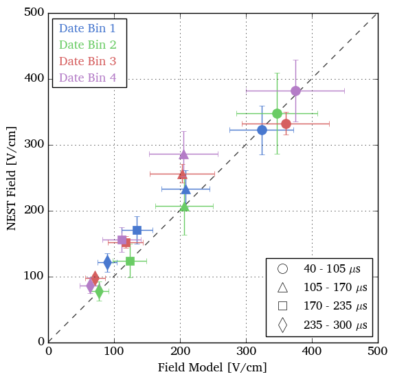
Figure 3.18: Comparison of the electric field as modeled using the COMSOL modeling method (“Field Model”) to the best fit predicted by NEST (“NEST Field”) for the 16 detector models (four drift time spatial regions and four time periods in date) used in the WS2014-16 analysis. Note that error bars on field map data points indicate the spread of the field within a bin.

3.3.3.7 Hand-off

Once the final charge distribution was found, the information included in the resulting field maps was provided on a $1\,\mathrm{cm^{3}}$ grid that included the detector real space coordinates $\left(x,y,z\right)$, the electric field in each location, and the coordinates as seen by the detector $\left(x_{S2},y_{S2},t\right)$. The transformation between real space and the reconstructed S2 space can be seen in the two plots in Figure 3.19. The field maps were then used in LUXSim simulations, position reconstruction, and limit-setting code for LUX searches for spin-independent and spin-dependent dark matter interactions [163, 127].

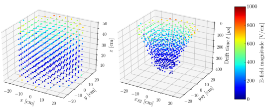
Figure 3.19: The transformation from the reconstructed S2 space (right) to real space (left). The color scale shows the electric field strength at each point using ${}^{\mathrm{83m}}\mathrm{Kr}$ data from 2015-08-26.

3.3.4 Time-dependence of electric fields during WS2014-16

3.3.4.1 Charge evolution

The method described here resulted in one field map for each month of WS2014-16, corresponding to 21 field maps in total. As discussed earlier, each field map was produced by adjusting the negative charge distribution in the PTFE panels and fitting the modeled electric field to the detector observables. One of the resulting charge distributions in the PTFE panels and the corresponding electric field is shown in Figure 3.20. The evolution of charge throughout WS2014-16 is demonstrated in Figure 3.21. The varying charge results in a time-dependent electric field, also changing in azimuth and $z$ as illustrated in Figure 3.22. The variability in $z$ can be explained by the difference of electron and hole mobility in the PTFE surfaces, while the non-uniformity in azimuth arises from the individual 12 PTFE panels exposure to varying intensity of VUV during the grid conditioning campaign.

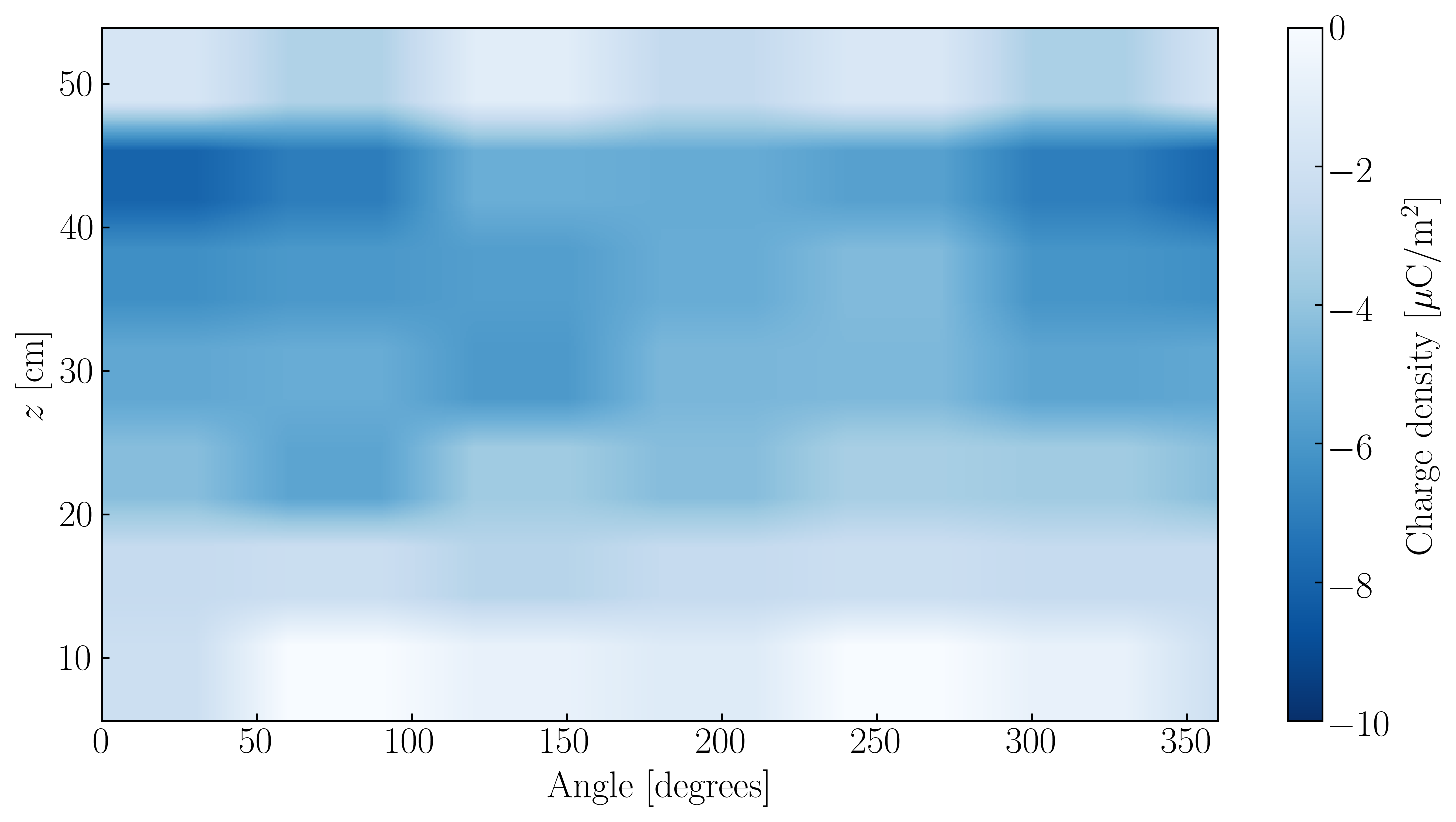
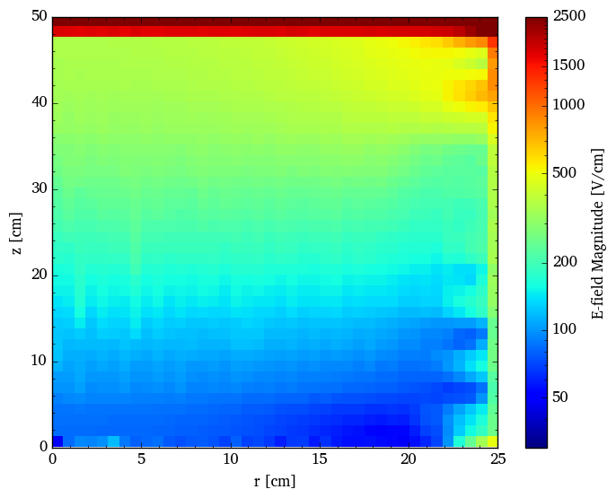
Figure 3.20: Left: Charge density distribution in the detector’s PTFE panels obtained from fitting ${}^{\mathrm{83m}}\mathrm{Kr}$ data from 2014-10-06. The 42 segments correspond to the smoothed tile charges described in Section 3.3.3.1. Right: Modeled electric field for the same dataset. The “bumps” at high $r$ are due to each panel having a slightly different charge and the smoothing algorithm not being quite perfect.

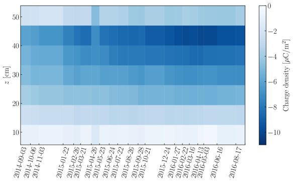
Figure 3.21: Charge density in each $z$ segment averaged over all azimuth throughout WS2014-16. Cathode is at $z=0$ and gate at $z=48.3\,\mathrm{cm}$.

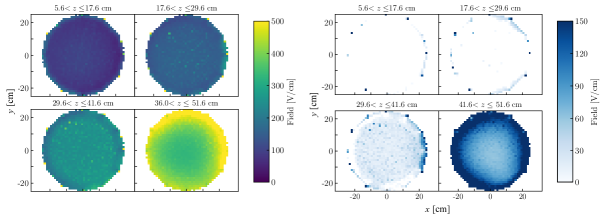
Figure 3.22: Left: The magnitude of electric field in different $z$ segments of the detector as modeled for 2014-09-03 dataset illustrating the azimuthal non-uniformity. Right: Difference between the electric field at the end of WS2014-16 (field map from 2016-05-03) and the beginning (field map from 2014-09-03). The change in field is not uniform throughout WS2014-16.

The most negative charge was found to be in the top $\nicefrac{{1}}{{3}}$ of the detector throughout all of WS2014-16, possibly due to hole states in the PTFE being pulled toward the cathode region, depleting the upper region first. Electron states may be moving upwards toward the gate, but at a slower rate. The increasingly negative charge throughout WS2014-16 averaged over the entire PTFE area is plotted in Figure 3.23. The cathode voltage was biased down to 0 V from April 7 to April 15, 2015, to investigate its effects on the charge in the PTFE panels; therefore, data from this period was not used in the analysis. Beginning after the cathode re-bias to −8.5 kV the charge density was fit with an exponential function corresponding to Equation 3.10 :

$$\sigma=\sigma_{0}\exp\left(-t/\tau\right)+\sigma_{\infty}$$ (3.14)

where $\sigma$ is the average surface charge density, $\sigma_{0}$ is the initial charge density, and $\sigma_{\infty}$ is the value of the charge $\lim_{t\rightarrow\infty}\sigma$. $\tau$ is the charge transit time. The best-fit values found were $\sigma_{0}=3.1\,\mathrm{\mu C/m^{2}}$, $\tau=181\,\mathrm{days}=1.6\times 10^{7}\,\mathrm{s}$, and $\sigma_{\infty}=\mathrm{\mu C/m^{2}}.-5.6\,\mathrm{\mu C/m^{2}}\,\mathrm{}$.

There is a lack of research of PTFE properties at LXe temperatures, so it is difficult to compare this number to the literature on PTFE charging. This is made even more difficult because of the experimental conditions used, such as surface cleanliness and the electric field applied.

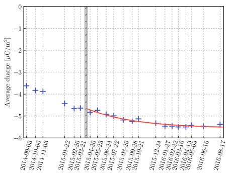
Figure 3.23: Increasingly negative charge density obtained from the field models averaged over the entire PTFE panel surfaces for each month during WS2014-16. The data points correspond to the modeled average charge densities in the PTFE panels obtained from a small subset of the regular ${}^{\mathrm{83m}}\mathrm{Kr}$ datasets. This data can be fitted with an exponential function $\sigma=3.1\exp\left(-t/181\right)-5.6$ where $t$ is in units of “days since 2014-09-03.” The gray dashed line indicates a week in April 2015 when the cathode voltage was biased down to 0 V.

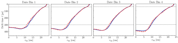
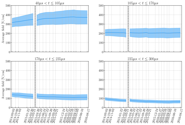
Figure 3.24: A comparison of the measured position of the detector wall and the cathode from ${}^{\mathrm{83m}}\mathrm{Kr}$ (solid blue) to that predicted by the best-fit electric field model (dashed red). Horizontal gray dashed lines, at 40 and 300 $\mu$s, indicate the drift time extent of the fiducial volume used in WS2014-16.

Figure 3.25: Average fields during WS2014-16 in the four drift time bins used in the analysis. Bands indicate the standard deviation of the field in the given drift time bin. A radial cut at $r=20\,\mathrm{cm}$ and a drift time cut at $40\,\mathrm{\mu s}<dt\leq 300\,\mathrm{\mu s}$ were applied. Gray dashed lines indicate a week in April 2015 when the cathode voltage was biased down to 0 V.

Date	Mean field [V/cm]	Standard deviation [V/cm]	Min field [V/cm]	Max field [V/cm]
2013-05-10	178	14	125	207
2014-09-03	194	89	45	487
2014-10-06	195	95	42	494
2014-11-03	196	96	38	503
2015-01-22	196	107	32	553
2015-02-26	197	111	43	560
2015-03-21	196	113	28	568
2015-04-26	197	106	44	576
2015-05-23	197	113	30	576
2015-06-24	199	117	21	584
2015-07-22	199	120	26	596
2015-08-26	199	121	29	606
2015-09-28	201	121	27	608
2015-10-21	199	123	24	607
2015-12-24	200	126	24	621
2016-01-27	201	129	19	635
2016-02-22	202	130	24	636
2016-03-16	202	131	20	641
2016-04-13	201	132	18	662
2016-05-03	200	130	18	637
2016-06-16	201	129	25	632
2016-08-17	201	128	23	631

Table 3.3: Field values throughout WS2014-16 in the fiducial volume (radial cut: $r\leq 20\,\mathrm{cm}$, drift time cut: $40\,\mu s<z<300\,\mu s$) calculated on a $1\,\mathrm{cm^{3}}$ grid found from the model. Data from 2013-05-10 is from WS2013 with radial cut $r\leq 20\,\mathrm{cm}$ and drift time cut $38\,\mu s<z<305\,\mu s$.

3.3.4.2 Electric fields in WS2014-16 analysis

As discussed in Section 2.4.4, for simplicity of the analysis in WS2014-16 the data were divided into 16 bins, within each of which the change in the wall position was not significant. There were four bins in time, bounded by the following dates: September 11, 2014; January 1, 2015; April 1, 2015; October 1, 2015; May 2, 2016. Each of those bins was further split into four drift time bins with boundaries of 40, 105, 170, 235, and 300 $\mu$s. These time bins used in the PLR analysis are coarser than the monthly fields maps. However, all field maps were used to inform a decision on the boundaries of these four time bins. Only one field map was chosen for each date bin; hence only four field maps were used in the WS2014-16 analysis. Each map was chosen to be close to the average of the electric field values in the segment. The agreement between each field map and a ${}^{\mathrm{83m}}\mathrm{Kr}$ distribution for each date bin is shown in Figure 3.25.

Figure 3.25 shows the value of the electric field throughout the WS2014-16 analysis; those values are also recorded in Table 3.3. The table shows a divergence of the field extrema as the electric field magnitude varied from $\sim 20-50\,\mathrm{V/cm}$ near the bottom of the detector to $\sim 500-650\,\mathrm{V/cm}$ near the top. The mean value of the field of $\sim 200\,\mathrm{V/cm}$ remained mostly constant throughout the exposure. The error on the values of electric fields obtained in this work is likely $\sim\pm 10\%$, the field variation needed to agree with simulation-data comparisons done at a later date based on charge and light signals.

3.4 Modeling small scale features

Despite the mostly uniform electric field in WS2013, the $\left(x,y\right)$ locations of S2 pulses did not have a dodecagonal outline as one might expect. Instead, small irregularities, referred to as “scalloping,” were observed along the edges of the detector that were not observed in the COMSOL Multiphysics model without charge in the PTFE surfaces, as shown in Figure 3.27.

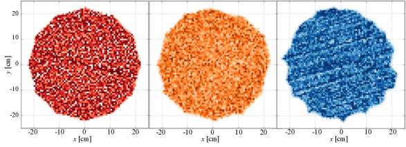
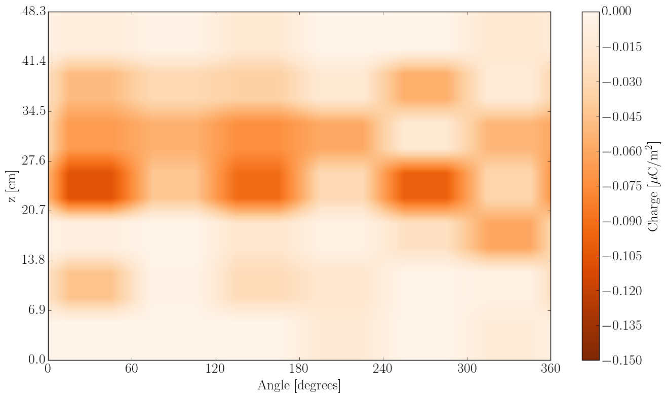
Figure 3.26: Left: Original COMSOL model with no charge showing a clear dodecagonal cross-section. Center: Data from the detector with visible scallops (most notably in the upper right quadrant and near the bottom) using ${}^{\mathrm{83m}}\mathrm{Kr}$ from 2013-05-10 taken during WS2013. Also visible is the orientation of gate wires. Right: COMSOL fit with charge included in the PTFE walls. The poor fit is likely due to only having six angular slices since the scalloping appears to be correlated with the individual detector PTFE panels. All cross-sections are a slice at a drift time of $255\,\mathrm{\mu s}<t\leq 290\,\mathrm{\mu s}$.

Figure 3.27: Charge distribution on the PTFE wall on 2013-05-10. The average charge on the wall is $-0.03\,\mathrm{\mu C/m^{2}}$, consistent with triboelectric charge densities.

Therefore, the same approach described in Section 3.3.3 to model electric fields in WS2014-16 was used to model this scalloping effect observed in WS2013. Since the tiling was optimized for WS2014-16, the model was unable to fully reproduce all the fine features, likely due to the bundling of the two adjacent PTFE panels together. The average fitted charge found in the PTFE panels was $-0.03\,\mathrm{\mu C/m^{2}}$ corresponding to $\sim 2\times 10^{5}\,\mathrm{e^{-}/mm^{2}}$, comparable to triboelectric charge densities as calculated in Section 3.4.2. In comparison, the charge densities simulated in WS2014-16 reached $-5.5\,\mathrm{\mu C/m^{2}}$. This illustrates the sensitivity of the field modeling method to capture even very small charge densities.

However, the scalloping feature in WS2013 appears to be more correlated with individual panels. Therefore the result could be improved by creating 12 angular section in the model. It is worth noting that increasing the number of angular sections would require a smaller amount of vertical divisions in the model since using, for example, 12 angular sections and 7 vertical divisions creates 84 tiles, which would more than double the already considerable computational complexity required by the Metropolis-Hastings algorithm to achieve convergence.

3.4.1 Wire grid spacing

One of the possible explanations for the scalloping features is variations in grid wire spacing. Figure 3.28 illustrates the effects of changing the distance between wires. Modifying this spacing alters the density of field lines passing between each wire pair, thus causing an effect throughout the length of the wire rather than being confined to the edge.

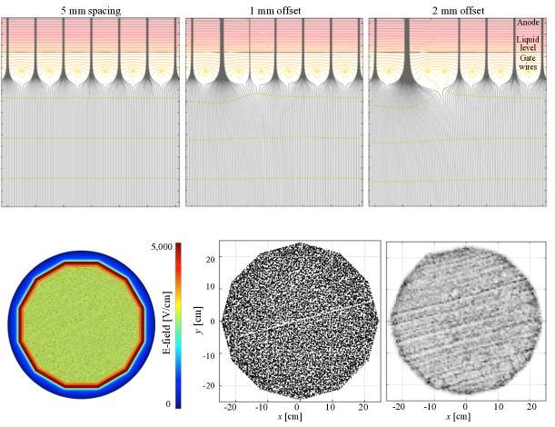
Figure 3.28: Top: Simulation of wire offset in the gate grid in WS2013 showing equipotentials at 50 V intervals (colored) and field lines (gray). Only field lines originating in the fiducial volume are shown indicating the path of electrons created in the detector. The left diagram shows the ideally parallel wires while the other two diagrams illustrate what happens when one wire is offset by 1 or 2 mm. A lateral offset can significantly vary the number of events “funneled” between a wire pair, up to completely stealing events from one gap to another. Figures modified from [280]. Bottom left: Electric field simulation from the COMSOL model as seen 1 mm above gate grid. The field “funnels” the field lines between the wires thus making the gate wires visible using the Mercury position reconstruction algorithm [208]. Dark red is the boundary of the grid frame, and the lighter red is where the grid wires pass through the PTFE wall. Bottom center: Simulation of particle distribution if one wire in the COMSOL model is shifted by 2 mm, resulting in a redirection of events from one gap to another. Events with drift time $<30\,\mathrm{\mu s}$ have been selected. Bottom right: ${}^{\mathrm{83m}}\mathrm{Kr}$ event density with the gate wires illuminated by the electrons. Events with drift time from $10\,\mathrm{\mu s}<t\leq 100\,\mathrm{\mu s}$ were selected. The overdensity of events at high radius is an artifact of the Mercury algorithm.

3.4.2 Static charge calculation

A simple back-of-the-envelope calculation can be performed to estimate the theoretical amount of excess charge needed to be transferred from, for example, a 1-g tissue paper, i.e., a Kimwipe, to the PTFE surface in order for the tissue paper to be attached to the PTFE surface electrostatically. Even though the electric charge found using charge modeling is not due to electrostatic charge (if it were, these electrons would follow the field lines and drift up to the gate rather than staying put), this provides an insight to the quantity of charge needed to produce such effects. The charge needed for the paper to hold on PTFE purely electrostatically needs to be at least equal to the gravitational force:

$$F = mg$$ (3.15)

$$= 1\times 10^{-3}\,\mathrm{kg}\times 9.8\,\mathrm{m/s^{2}}=9.8\times 10^{-3}\,\mathrm{N}$$ (3.16)

$$= \frac{1}{4\pi\varepsilon_{0}}\frac{q_{1}q_{2}}{r^{2}}.$$ (3.17)

Electrons transferred to PTFE must be equal to the positive charges left on the wipe, so $q_{1}q_{2}=q^{2}$ and $r$ is the distance between point charges, which is assumed here to be only $\sim 0.1\,\mathrm{mm}$. Therefore

$$q = \sqrt{4\pi\varepsilon_{0}Fr^{2}}$$ (3.18)

$$= \sqrt{4\pi*8.85\times 10^{-12}\times 9.8\times 10^{-3}\times\left(0.1\times 10^{-3}\right)^{2}}$$ (3.19)

$$= 1.0\times 10^{-4}\,\mathrm{\mu C}.$$ (3.20)

Assuming the mass of the tissue paper to be $\sim 40\,\mathrm{g/m^{2}}$, $1\,\mathrm{g}$ of tissue paper has an area of $\sim 250\,\mathrm{cm^{2}}$. Hence this charge corresponds to a surface charge density of $4\times 10^{-7}\,\mathrm{\mu C/cm^{2}}=0.004\,\mathrm{\mu C/m^{2}}$. Thus the charge observed in WS2013 in the PTFE panels surrounding the active volume is only slightly larger than typical static charge.

3.5 Future avenues of research

Since the field maps laid the foundation for the rest of the WS2014-16 analysis, the timeline of this project was constrained in order to provide the complete field maps on time to the rest of the LUX collaboration. Therefore compromises were made throughout the project to abide by the tight WS2014-16 analysis schedule. Nevertheless, the models developed here show good agreement with charge, light, and event positions observed in LUX data.

A significant factor in the quality of the models and the speed of convergence was given by the number of divisions on the PTFE panels used. The initial 15 tiles used in this work (3 angular and 5 vertical sections, without the smoothing function) provided a model that was too coarse. However, this worked as a proof of concept since the model converged during tests to a known charge distribution on the PTFE panels. The next model built consisted of 42 charge tiles (6 angular and 7 vertical sections with the smoothing function). This allowed for a better fidelity fit, however, the increased complexity of the model due to the large number of free parameters caused a very slow convergence of the Metropolis-Hastings algorithm, and a perfect fit was never reached. Slightly different sectioning of the detector might have been preferable, such as using only 4 angular and 6 or 7 vertical slices, resulting in 24 or 28 tiles and thereby significantly decreasing the number of free parameters while retaining a good resolution.

Better coding of the simulated drifting electrons would have also improved fitting results. Improvements in time efficiency and therefore accuracy could likely come from efforts focused on reducing the algorithmic complexity class, effective parallelization of the computation, and using a compiled programming language such as C/C++ rather than Python.

3.6 Conclusion

The above method for detailed modeling of the varying electric fields inside the active volume of the LUX detector enabled understanding of the electric fields. This was vital for event reconstruction and hence served as the foundation of the LUX WIMP search analysis. The fields observed in the bulk of the active volume of the detector during WS2013 were reproduced without any tuning necessary. The COMSOL field map modeling method described in this work is sensitive down to $-0.03\,\mathrm{\mu C/m^{2}}$, enough charge density to model minor scalloping to the detector edge as seen in WS2013.

The time dependence of the electric field during WS2014-16 was likely due to the creation of charge in the PTFE panels during detector grid conditioning prior to the extended scientific run. The model of electric fields was created by simulating the LUX detector in 3D using COMSOL Multiphysics with the PTFE panels divided into 42 tiles. The use of superposition principle then enabled placement of any combination of hypothetical charges on the PTFE panels surrounding the active region. The amount of charge on each tile was varied until convergence on the distribution of ${}^{\mathrm{83m}}\mathrm{Kr}$ calibration data within the detector was obtained. The resulting method allowed a faithful reconstruction of electric fields in the LUX detector. The fields during WS2014-16 varied in time, azimuth and depth; the method described in this work was able to capture this evolution in all dimensions. Twenty-one field maps were developed to accurately model the changing electric field throughout the extended WS2014-16 with an average modeled charge distribution in the PTFE panels varying from $-3.6\,\mathrm{\mu C/m^{2}}$ to $-5.5\,\mathrm{\mu C/m^{2}}$.

The mean electric field values resulting from this COMSOL modeling method were found to be in good agreement with electric field values deduced from the NEST package, which fit the field-dependent scintillation and ionization yields of the CH₃T calibration source. This work also improved understanding of the cathode grid geometry on the field leakage and its effect on axially symmetric models. The successful modeling of electric fields, along with the robust calibration and simulation programs developed by the LUX collaboration enabled a thorough understanding of the LUX detector throughout all of its scientific programs and strengthened its sensitivity to WIMPs.

Chapter 4 Searching for sub-GeV dark matter with the LUX detector

The two-phase xenon time projection chamber (TPC) is the leading technology used to search for the weakly interacting massive particle (WIMP), a favored dark matter (DM) candidate, in the $5\,\mathrm{GeV/c^{2}}$ to $10\,\mathrm{TeV/c^{2}}$ mass range. Despite substantial improvements in sensitivity over the recent years, detecting DM remains an elusive goal [163, 102, 164]. Consistent progress in ruling out WIMP parameter space has resulted in a significant broadening of efforts, including focusing on lighter particles as possible DM candidates. Currently, the intrinsic scintillation properties of nuclear recoils prevent liquid xenon (LXe) TPCs to reach sub-GeV DM masses, for analyses based on both S1 and S2 signals. Lower thresholds can be achieved in S2-only studies [281] that drop the requirement for the scintillation (S1) signal since charge yields are higher at low energies. However, this type of analysis is currently limited by anomalous few-electron background, which prevents construction of a complete background model, impairing dark matter detection claims.

Recently, References [282, 283] proposed novel direct dark matter detection methods that extend the reach of LXe detectors to sub-GeV DM masses. They suggest that DM-nucleus scattering can be accompanied by a signal that results in an electron recoil at higher energies than the corresponding nuclear recoil in LXe detectors. Since electron recoils (ER) produce a stronger signal than nuclear recoils at low energies, this newly recognized channel enables liquid xenon detectors to reach sub-GeV DM masses. In LUX the 50% detection efficiency for nuclear recoils is 3.3 keV, compared with 1.24 keV for electron recoils.

This chapter discusses searches of sub-GeV DM in the LUX detector using two different mechanisms: Bremsstrahlung, first proposed in [282], and the Migdal effect as reformulated in [283]. These inelastic signals produce much stronger charge and light yields compared to the traditional elastic recoil signal for DM candidates with masses below $\sim 5\,\mathrm{GeV/c^{2}}$.

Bremsstrahlung considers emission of a photon from the recoiling atomic nucleus. In the atomic picture, the process can be viewed as a dipole-emission of a photon from a xenon atom polarized in the DM-nucleus scattering. The Migdal effect describes the ionization of an atom as a result of a sudden acceleration of a recoiling nucleus after a collision. This creates an ER response alongside its nuclear recoil. Considering photons from Bremsstrahlung or electrons from the Migdal effect allows LUX to access sub-GeV DM parameter space. Both the S1 and the S2 signals can be used in the analysis where the nuclear recoil signal would not be visible otherwise, extending the reach of liquid xenon detectors to lower masses of DM particles than has been achieved previously in S1-S2 analyses. This analysis also provides sensitivity to lower masses than S2-only analysis [281] of nuclear recoils.

This chapter first provides an overview of the scattering rate calculations for the Bremsstrahlung and Migdal effects. Several different mediator scenarios are considered for the two effects. The predicted scattering rates are then applied in the analysis to place limits on DM-nucleon scattering cross section. The results presented in this chapter have also been accepted for publication to PRL [151].

4.1 Bremsstrahlung

As was first postulated in [282], two-phase LXe TPC can search for sub-GeV dark matter using an irreducible photon emission in the form of bremsstrahlung from a polarized xenon atom, caused by the displacement of the nucleus and electron charges after the DM - nucleus interaction. The most common, elastic interaction between DM $\chi$ with mass $m_{\chi}$ and nucleus $N$ with mass $m_{N}$ considers

$$\chi+N\rightarrow\chi+N\left(E_{R}\right).$$ (4.1)

Here $E_{R}$ is the kinetic energy of the recoiling nucleus with momentum $\mathbf{q}=\mathbf{p^{\prime}_{\chi}}-\mathbf{p_{\chi}}$ given by

$$E_{R}=\frac{\left|\mathbf{q}\right|^{2}}{2m_{N}}\leq\frac{2\mu_{N}^{2}v^{2}}{m_{N}}$$ (4.2)

where $\mu_{N}$ is the DM-nucleus reduced mass

$$\mu_{N}=\frac{m_{N}m\chi}{m_{N}+m_{\chi}}$$ (4.3)

and $v$ is the relative velocity. For an inelastic interaction

$$\chi+N\rightarrow\chi+N\left(E_{R}^{{}^{\prime}}\right)+\gamma\left(\omega\right)$$ (4.4)

where the available photon energy $\omega\leq\mu_{N}v^{2}/2$ as bounded by the energy of the relative motion of DM and the target restricts the kinetic energy of the recoiling nucleus $E_{R}\ll\omega_{max}$ for $m_{\chi}\ll m_{N}$. This larger energy deposition in photon emission improves the sensitivity of LUX to nuclear recoils in the sub-GeV DM mass regime. The emitted photon from the recoiling nucleus has a continuous energy spectrum, exciting and ionizing surrounding xenon atoms and resulting in an ER signal. However, this signal is weaker compared to the standard nuclear elastic scattering since a penalty is paid for going to the inelastic channel. Additionally, in LXe TPCs most background events fall within the ER band. This means that it will be subject to a higher amount of backgrounds while having a significantly lower detection threshold.

The scattering rates for Bremsstrahlung $\frac{dR}{d\omega}$ have been derived [282], and a short outline follows. The differential cross section for a bremsstrahlung emission from the nucleus in the presence of an electron cloud is given by

$$\frac{d^{2}\sigma}{d\omega dE_{R}} =\frac{4\alpha}{3\pi\omega}\frac{E_{R}}{m_{N}}\left|f\left(\omega\right)\right|^{2}\times\frac{d\omega}{dE_{R}}\Theta\left(\omega_{\mathrm{max}}-\omega\right)$$

$$\propto\omega^{3}.$$

Here $\alpha=1/137$ is the fine structure constant, characterizing the strength of the electromagnetic interaction between elementary charged particles. The atomic form (or scattering) factor $f\left(\omega\right)=f_{1}\left(\omega\right)+if_{2}\left(\omega\right)$ is the Fourier transform of the electron density of an atom which measures the scattering amplitude of a wave by an isolated atom. Generally, the electron density is assumed to be spherically symmetric so that the value of the Fourier transform only depends on the distance from the origin in reciprocal space. The case of xenon is illustrated in Figure 4.1. At large energies, $f_{1}\rightarrow Z\gg f_{2}$, and the atomic states become irrelevant, where $Z$ is the atomic number. At low photon energies, the process weakens as $\omega^{3}$, which is typical for dipole emission created between the nucleus and electrons. To simplify the atomic calculations, Reference [282] assumes that the atom stays in the ground state. Therefore, the limits presented below should be considered conservative. More detailed calculations of the atomic processes are left for future research, potentially leading to an increase in the photon signal.

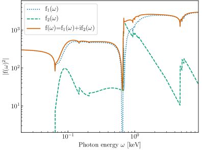
Figure 4.1: Xenon atomic scattering factor $f\left(\omega\right)=f_{1}\left(\omega\right)+if_{2}\left(\omega\right)$. Data from [284].

To find an expression for the differential event rate seen in the detector, the energy deposition $E_{R}$ is neglected since

$$E_{R,\mathrm{max}}=4\frac{m_{\chi}}{m_{N}}\omega_{\mathrm{max}}\ll\omega_{\mathrm{max}} \quad\mathrm{for}\>m_{\chi}\ll m_{N}.$$ (4.5)

Therefore, the photon energy is treated as the only detectable quantity with

$$\frac{d\sigma}{d\omega}=\int_{E_{R,\mathrm{min}}}^{E_{R,\mathrm{max}}}dE_{R}\left(\frac{d\sigma}{dE_{R}d\omega}\right)$$ (4.6)

where the DM-nucleus recoil cross section is

$$\frac{d\sigma}{dE_{R}}=\frac{\sigma_{0}^{\mathrm{SI}}m_{N}}{2\mu_{N}^{2}v^{2}}F_{N}^{\mathrm{SI}}\left(E_{R}\right)F_{\mathrm{med}}\left(E_{R}\right).$$ (4.7)

Here $\sigma_{0}^{\mathrm{SI}}$ is the usual DM-nucleon spin-independent cross section

$$\sigma_{0}^{SI}\simeq\sigma_{n}\left(\frac{\mu_{N}}{\mu_{n}}\right)^{2}A^{2}$$ (4.8)

where $\sigma_{n}$ is the DM-nucleon elastic cross section, and $\mu_{n}$ is the DM-nucleon reduced mass (cf. Equation 1.18). Note that $\sigma_{n}$ and $m_{\chi}$ form precisely the parameter space that DM searches, including LUX, are attempting to probe. $F_{N}^{\mathrm{SI}}\left(E_{R}\right)$ is the nuclear form factor that is relevant when the wavelength $h/q$ is no longer large compared to the nuclear radius as discussed in Section 1.3.3.1. The form factor is unity for small $q$, and it decreases with increasing $q$. The form factor is a function of the dimensionless quantity $qr_{n}/\hbar$, where $r_{n}$ is an effective nuclear radius and $\hbar=h/\left(2\pi\right)$ is the reduced Planck constant. Different approximations can be used to calculate the nuclear form factor; this analysis adopts the Helm form factor discussed in [77]. $F_{\mathrm{med}}$ depends on the mass of the particle mediating the interaction discussed in Sections 4.1.1 and 4.1.2.

The differential cross section can be integrated to yield

$$\frac{d\sigma}{d\omega}=\frac{4\alpha\left|f\left(\omega\right)\right|^{2}}{2\pi\omega}\frac{\mu_{N}^{2}v^{2}\sigma_{0}^{\mathrm{SI}}}{m_{N}^{2}}\sqrt{1-\frac{2\omega}{\mu_{N}v^{2}}}\left(1-\frac{\omega}{\mu_{N}v^{2}}\right).$$ (4.9)

The resulting event rate is then given by

$$\frac{dR}{d\omega}=N_{T}\frac{\rho_{\chi}}{m_{\chi}}\int_{\left|\mathbf{v}\right|\geq v_{min}}d^{3}\mathbf{v}vf_{v}(\mathbf{v}+\mathbf{v_{e}})\frac{d\sigma}{d\omega}.$$ (4.10)

Here $N_{T}$ is the number of target nuclei per unit detector mass and $\rho_{\chi}=0.3\,\mathrm{GeV/cm^{3}}$ is the local DM mass density. $f_{v}\left(\mathbf{v}\right)$ is the DM velocity distribution represented by a truncated Maxwellian

$$f_{v}\left(\mathbf{v}\right)=\begin{cases}\frac{1}{N_{esc}}\left(\frac{3}{2\pi\sigma_{v}^{2}}\right)^{3/2}e^{-3\mathbf{v^{2}}/2\sigma_{v}^{2}}&\mathrm{for}\,\left|\mathbf{v}\right|<v_{esc}\\ 0&\mathrm{otherwise}\end{cases}$$ (4.11)

where

$$N_{esc}=\frac{\mathrm{erf}\left(z\right)-2z\exp\left(-z^{2}\right)}{\sqrt{\pi}}$$ (4.12)

with the normalization factor $z\equiv v_{esc}/v_{0}$. In this analysis, the escape speed $v_{esc}=544\,\mathrm{km/s}$, $\mathbf{v}_{e}=232.4\,\mathrm{km/s}$ is the velocity of the Earth relative to the Galactic rest frame, $v_{min}=\sqrt{2\omega/\mu_{N}}$, and the most probable velocity $v_{0}=\sqrt{2/3}\sigma_{v}=220\,\mathrm{km/s}$ [157].

The goal of the analysis presented in this chapter is to apply the theoretical scattering rates from Bremsstrahlung presented in Equation 4.10 and from the Migdal effect introduced in the next section to the data acquired during LUX WS2013. Several different mediator scenarios are considered. This analysis will determine whether LUX has observed DM in the sub-GeV region.

4.1.1 Heavy scalar mediator

A mediator defines the coupling between the DM and Standard Model (SM) particles. Different mediators can enter Equation 4.7. A scalar mediator couples to SM particles by mixing with the SM Higgs boson making its coupling proportional to the particle’s mass $A$ (equal interaction strength with protons and neutrons).

The other factor in Equation 4.7, $F_{med}\left(E_{R}\right)$, depends on the mass of the particle mediating the interaction. In the heavy mediator limit $m_{med}\gg q$ and the mediator factor can be well approximated as $F^{2}\simeq 1$ at low energies.

4.1.2 Light scalar mediator

Aside from the common heavy scalar mediator case, a light scalar mediator is considered where $m_{\mathrm{med}}\ll q$ results in $F_{\mathrm{med}}=q_{\mathrm{ref}}^{4}/q^{4}$. We define $q_{\mathrm{ref}}=1\,\mathrm{MeV}$, a typical size of $q$ for $m_{\chi}\lesssim 1\,\mathrm{GeV/c^{2}}$ [80]. The resulting event rates for both light and heavy scalar mediator are shown in Figure 4.2 along with the conventional elastic scattering rate. This plot illustrates the comparative advantage that the Bremsstrahlung signal offers at low dark matter masses: the nuclear recoils resulting from the SI scattering rate are otherwise inaccessible due to the finite detector threshold (set at 1.1 keV as discussed in Section 2.4.2).

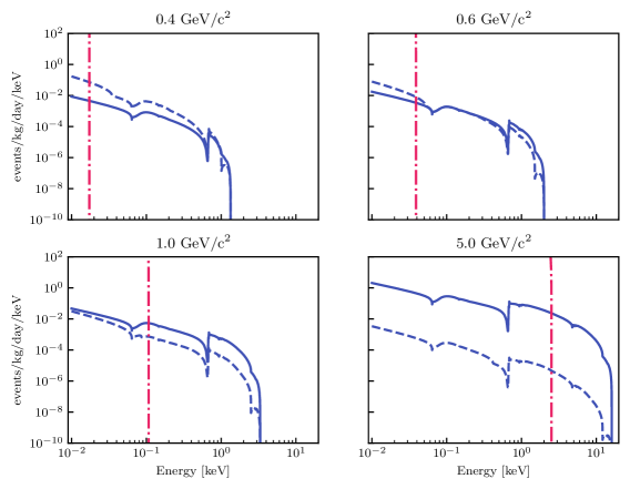
Figure 4.2: SI scattering rates in xenon for Bremsstrahlung that would be detected as electron recoils in LUX assuming $\sigma=1\times 10^{-35}\,\mathrm{cm^{2}}$. Two different mediators are considered: a heavy scalar mediator ($m_{med}\gg\mathrm{MeV}$, solid blue) and light mediator ($m_{med}\ll\mathrm{MeV}$ where $q_{\mathrm{ref}}=1\,\mathrm{MeV}$, dashed blue). To illustrated the improvement in reach for LXe detectors that Bremsstrahlung presents, the scattering rates resulting in nuclear recoil calculated in Equation 1.21 are also shown (dash-dot pink). The NR threshold in LUX is 1.1 keV.

4.2 Migdal effect

For nuclear recoils in liquid xenon, it is usually assumed that electrons around the recoiling nucleus immediately follow the motion of the nucleus so that the atom remains neutral. In reality, it takes some time for the electrons to catch up, which may result in ionization and excitation of the atoms [283], as illustrated in Figure 4.3. When A.B. Migdal originally formulated the Migdal effect in 1941 [285], he assumed an impulsive force to justify his calculations [286]. In his original approach, the final state ionization and excitation are treated separately from the nuclear recoil, which makes energy-momentum conservation and probability conservation somewhat obscure.

However, reference [283] has reformulated the approach using atomic energy eigenstates for their calculation (rather than the energy eigenstates of the isolated nucleus), avoiding the need to resolve the complex time evolution of the nucleus-electron system. In this way, the atomic recoil cross section is obtained coherently, and energy-momentum conservation and probability conservation are manifest in the final state. A DM-nucleus interaction is expected to cause a non-vanishing overlap between the initial and final atomic energy states, which result in the excitation and the ionization processes. It should be noted that the Migdal effect is distinct from the ionization and scintillation process since the Migdal effect takes place even for a scattering of an isolated atom, while the latter occurs due to the interatomic interactions in the xenon detector. Reference [283] contains the theoretical derivation and presents expected event rates for the Migdal effect; only a brief summary of that manuscript is presented below.

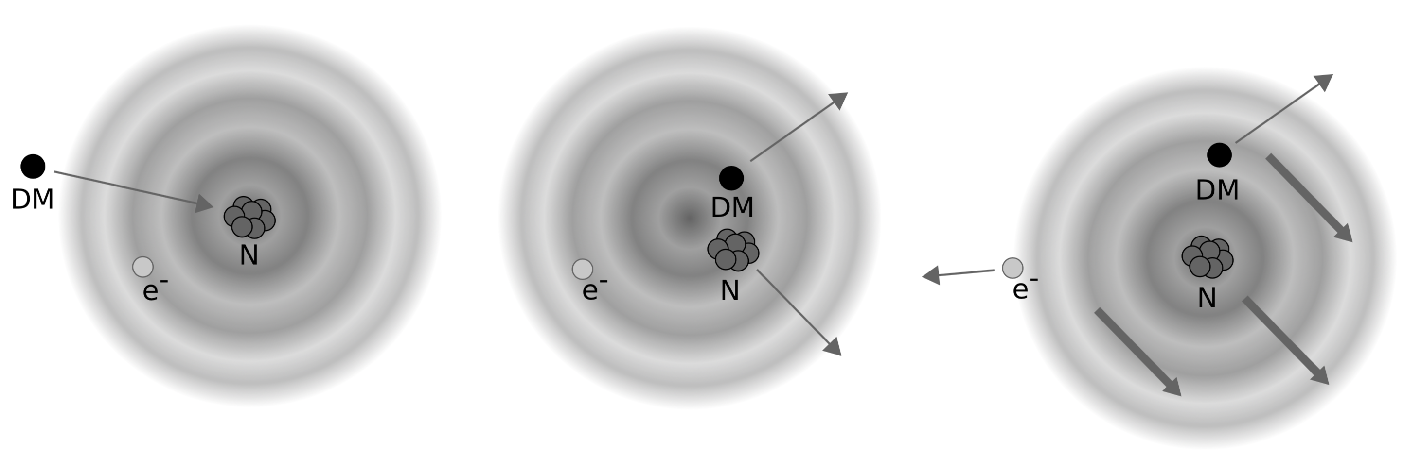
Figure 4.3: Illustration of a nuclear recoil causing an electron emission due to the Migdal effect. After a DM particle scatters off a nucleus (left), the Migdal effect assumes that the nucleus moves relative to its surrounding electron cloud (center). Most electrons catch up with the nucleus, but some electrons may be left behind and are emitted, leading to ionization and excitation of the recoiling atom (right). Figure from [287].

The ionized electronic energy spectrum from an initial orbital $o_{k}$ is given as a product of the dark matter event rate for unit detector mass $dR_{0}/dE_{R}dv_{\chi}$ and the differential ionization probability $dp_{q_{e}}^{c}/dE_{e}$ of the bound states $\left(n,\ell\right)$ (shown in Figure 4.4):

$$\frac{dR}{dE_{R}dE_{e}dv_{\chi}}\simeq \frac{dR_{0}}{dE_{R}dv_{\chi}}\times\frac{1}{2\pi}\sum_{n,l}\frac{d}{dE_{e}}p_{q_{e}}^{c}\left(n\ell\rightarrow E_{e}\right)$$ (4.13)

where the dark matter event rate for unit detector mass

$$\frac{dR_{0}}{dE_{R}dv_{\chi}}\simeq \frac{1}{2}\frac{\rho_{\chi}}{m_{\chi}}\frac{1}{\mu_{N}^{2}}\tilde{\sigma}_{N}\left(q_{A}\right)\times\frac{\tilde{f}\left(v_{\chi}\right)}{v_{\chi}},$$ (4.14)

$\tilde{f}\left(v_{\chi}\right)$ is the DM velocity distribution integrated over the directional component normalized by $\int\tilde{f}_{\chi}\left(v_{\chi}\right)dv_{\chi}=1$, and $\tilde{\sigma}_{N}=\sigma_{0}^{SI}F_{N}^{\mathrm{SI}}F_{\mathrm{med}}$. The atomic recoil energy $E_{R}$ is given by

$$E_{R}\simeq \frac{q_{A}^{2}}{2m_{A}}$$ (4.15)

$$q_{e}\simeq \frac{m_{e}}{m_{A}}q_{A}$$ (4.16)

where $q_{A}$ is the momentum transfer of the recoil, $m_{e}$ is the mass of the electron, and $m_{A}$ is the mass of the atom. The minimum dark matter velocity for given $E_{R}$ and $\Delta E$

$$v_{\chi,min}\simeq\frac{m_{N}E_{R}+\mu_{N}\Delta E}{\mu_{N}\sqrt{2m_{N}E_{R}}}$$ (4.17)

which determines the kinematically allowed region of $E_{R}$.

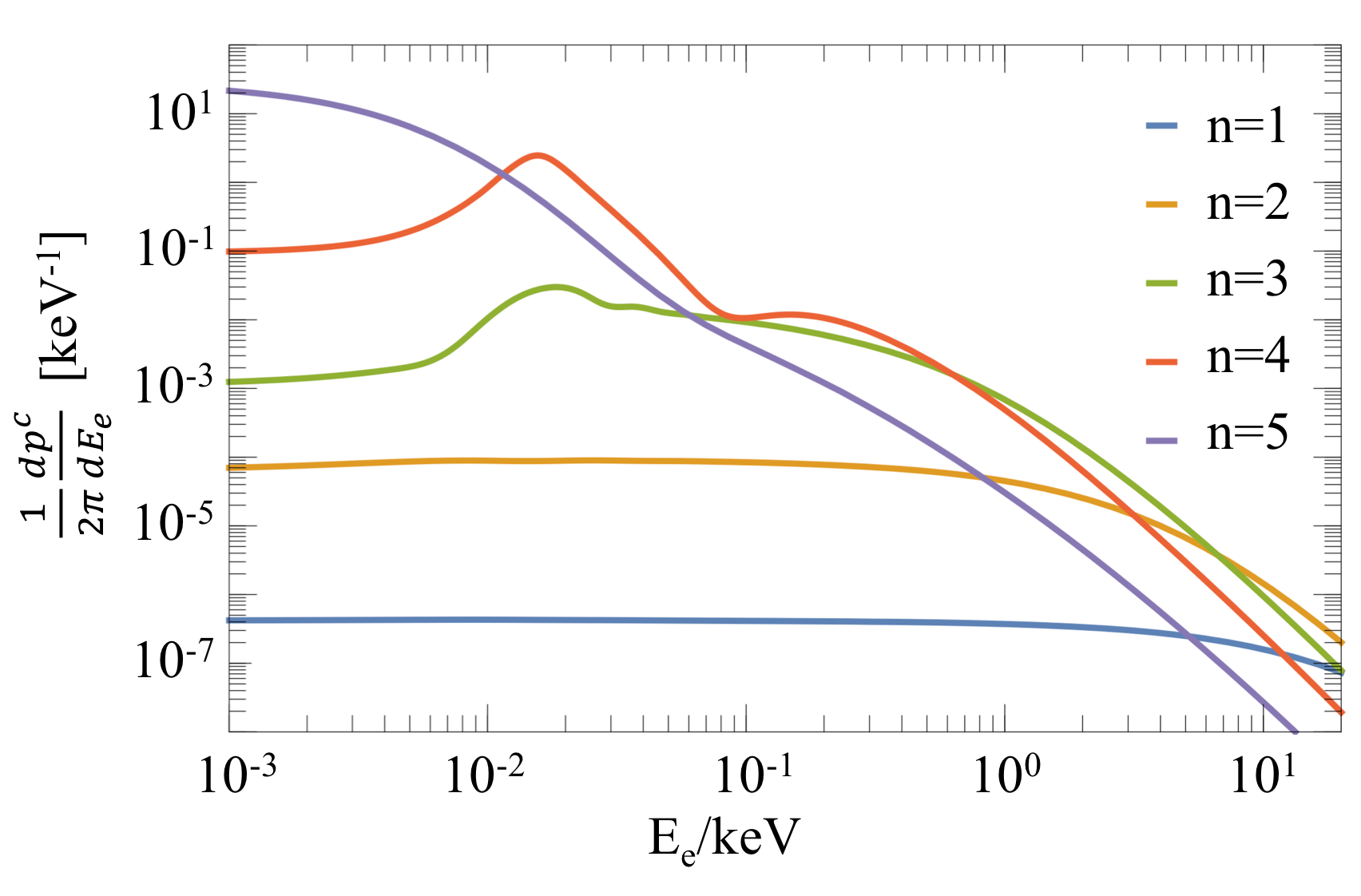
Figure 4.4: Differential ionization probabilities as a function of the emitted electronic energy $E_{e}$ for isolated xenon atom for $q_{e}=m_{e}v_{F}$ with the velocity after the recoil $v_{F}=10^{-3}$. The contributions from different $\ell$ and the possible final states for a given $n$ are summed. Figure modified from [283].

Figure 4.5 contains the scattering rates derived in Equation 4.13 for a given SI scattering cross section of DM on nucleons, showing contributions from electrons from the various atomic shells. Only electron injections caused by ionization are included since the excitation probabilities into the unoccupied binding energy levels are much smaller than the ionization probabilities. Additionally, the derivation in [283] assumes isolated atoms, so additional considerations need to be made for non-isolated atoms in liquid or crystals. In non-isolated atoms, such as in liquid xenon, the energy levels of valence electrons in $n=5$ states are affected by the ambient atoms by $\mathcal{O}\left(0.1\right)\,\mathrm{eV}$. In comparison, the ionization rates from the inner orbitals are expected to be less affected by ambient atoms since the binding energies of inner orbitals are much larger than 0.1 eV. Thus, this analysis conservatively ignores the contribution from electrons in $n=5$ states. The ionization spectrum in Equation 4.13 can be applied rather reliably for electrons from the inner orbitals with $n=3,4$ [283]. Electrons from $n=1$ require ionization energy of about 35 keV and begin to contribute at DM masses of $\sim 10\,\mathrm{GeV/c^{2}}$. At lower masses, DM requires speeds higher than the escape velocity. Contributions to the signal from $n=2$ electrons need ionization energy of $\sim 5\,\mathrm{keV}$ and become visible at DM masses of $\sim 2\,\mathrm{GeV/c^{2}}$, but the size of the signal is minimal. Therefore, contributions to the signal model from $n=1,2$ orbitals are neglected since their contribution is negligible at DM masses considered here.

Figure 4.5 also illustrates that the energy from the ionization can be larger than the nuclear recoil energy from the elastic scattering alone for light DM. For heavier dark matter, $m_{\chi}>\mathcal{O}\left(10\right)\,\mathrm{GeV/c^{2}}$, on the other hand, the Migdal effect is submerged below the conventional nuclear recoil spectrum, and hence, does not affect the detector sensitivities. In principle, the additional electronic energy injections affect the S2/S1 ratio in the detector.

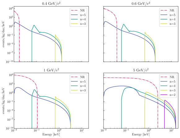
Figure 4.5: Scattering rates in xenon from the Migdal effect showing contributions from electrons shells. Contributions from $n=1,\,2$ are not relevant for the DM masses plotted here except at $5\,\mathrm{GeV/c^{2}}$. Since the derivation assumes isolated atoms, the ionization spectrum from the valence electrons, i.e., $n=5$, are not reliable. The analysis thus uses only electrons from $n=3,\,4$. The DM-nucleus scattering rates resulting in elastic nuclear recoil in LUX are also shown (dash-dot pink).

It should be emphasized that both the nuclear and electron recoil signals are present when considering the Bremsstrahlung and Migdal effects. However, the nuclear recoil signal from sub-GeV DM is undetectable by LUX, so only the electron recoil signal is used in this analysis. Higher interaction rates in the region of interest are expected from the Migdal effect than Bremsstrahlung as shown in Figure 4.6.

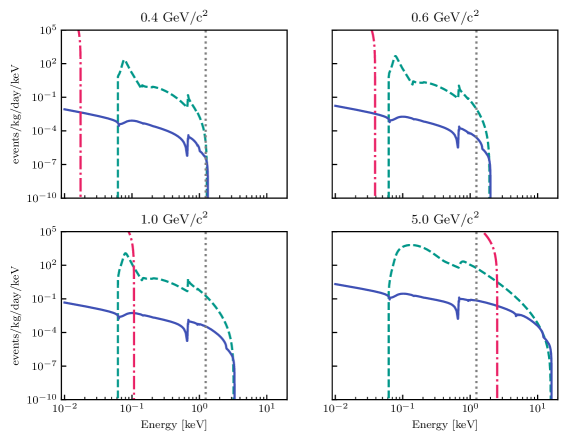
Figure 4.6: Scattering rates in xenon for Bremsstrahlung (solid blue) and Migdal effect (dashed teal) illustrating the suppression of Bremsstrahlung by the mass of the nucleus resulting in lower scattering rates. The DM-nucleus scattering rates resulting in elastic nuclear recoil in LUX are also shown (dash-dot pink). Also shown is a signal cut off at 1.24 keV (dotted gray) applied in the analysis, corresponding to 50% efficiency of ER detection (see Section 4.3.1). Note that 50% efficiency for NR event detection occurs at 3.3 keV [187].

4.2.1 Vector mediator

Unlike the scalar mediator whose coupling is proportional to the particle’s mass, the vector mediator couples to SM particles via mixing with the SM photon, making its coupling proportional to the particle’s electromagnetic charge. These so-called dark photon models result in a $Z^{2}$ enhancement for scattering on nuclei with charge number $Z$ and have comparable couplings to protons and electrons [287].

Additionally as mentioned in Section 4.1.2, both light and heavy mediator cases were considered. Overall this results in up to 4 different limits for each of the signal models as illustrated in Figure 4.7 for the case of the Migdal effect.

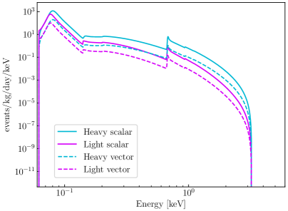
Figure 4.7: Scattering rates in xenon from Migdal effect for various mediator cases at $\sigma=1\times 10^{-35}\,\mathrm{cm^{2}}$ for $1\,\mathrm{GeV/c^{2}}$ dark matter. The scalar mediator’s coupling is proportional to the recoiling particle’s mass $\left(\sigma_{N}\propto A^{2}\right)$, while the vector mediator’s coupling is proportional to the particle’s electromagnetic charge $\left(\sigma_{N}\propto Z^{2}\right)$. For the heavy mediator $m_{med}\gg q$, while for the light mediator $m_{\mathrm{med}}\ll q$ where we define $q_{\mathrm{ref}}=1\,\mathrm{MeV}$ where $q$ is the momentum transfer.

4.3 Analysis

LUX collected data during two scientific searches in 2013 [101, 187] and in 2014-16 [163]. The work presented here uses WIMP search data with a total exposure of 95 live-days using 118 kg of LXe in the fiducial volume collected from April 24 to September 1, 2013, referred to as WS2013 presented in [187] and discussed in Section 2.4.2. Only single scatter events (one S1 followed by one S2) are considered with analysis cuts summarized in Table 2.3 with detector-specific gain factors $g_{1}=0.117$ detected photons (phd) per photon emitted and $g_{2}=12.2\,\mathrm{phd}$ per electron.

4.3.1 Detector response to electron recoils

The response of the LUX detector to ERs was characterized using internal tritium calibrations performed in December 2013, directly following WS2013. Tritiated methane CH₃T was injected into the gas circulation to achieve a spatially uniform distribution of events dissolved in the detector’s active region as described in [182] and discussed in Section 2.2.6.2. This direct calibration is then used to build the signal model used in this analysis. Figure 4.8 shows excellent agreement between the ER yields from the in situ tritium calibrations and yields obtained from the Noble Element Simulation Technique (NEST) package v2.0 [185, 230, 288, 231], used to model the ER response in the signal model. The complementary behavior between light and charge yields is due to recombination effects described in [182, 179]. Since this work considers recoils at the lowest energies, it can be seen in Figure 4.8 that the analysis is limited by light production rather than charge yields. Also, the efficiency for extracting electrons from liquid to gas $\varepsilon=49\%\pm 3\%$ while the aforementioned efficiency to detect S1 photons $g_{1}=\left(0.117\pm 0.003\right)\,\mathrm{phd}$ per photon.

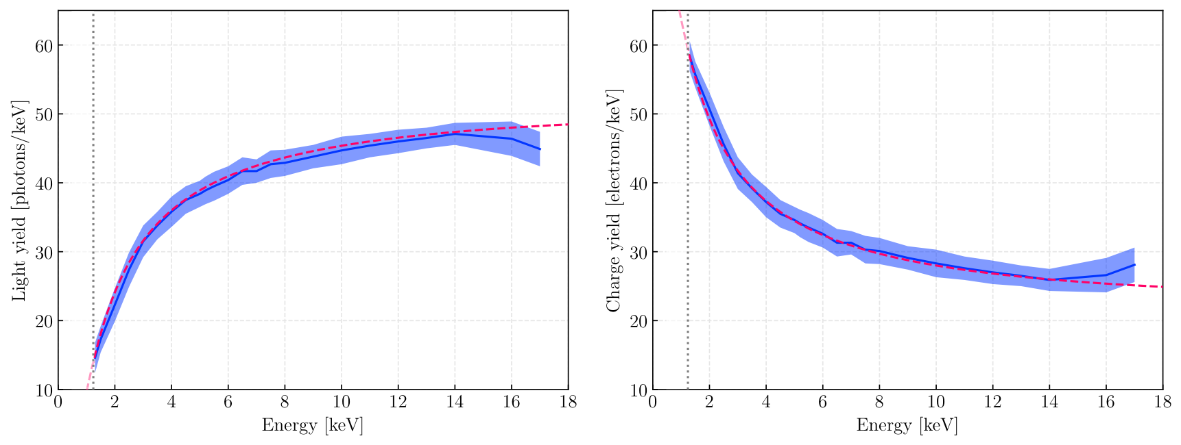
Figure 4.8: The light (left) and charge yields (right) of tritium ER events as a function of recoil energy measured in situ by the LUX detector at 180 V/cm (solid blue line) compared to NEST v2.0 (dashed pink line). The bands indicate the 1 $\sigma$ uncertainties on the measurement. The gray dotted line shows the 1.24 keV threshold implemented in the analysis.

A 1.24 keV low-energy cutoff illustrated in Figure 4.6 was conservatively chosen to avoid uncertainties in efficiency at low energy, where direct calibration data from tritium are not available. 1.24 keV corresponds to a 50% efficiency of ER detection (cf. Figure 2.20), which imposes a lower limit on DM mass of $0.4\,\mathrm{GeV/c^{2}}$. The upper DM mass boundary of $5\,\mathrm{GeV/c^{2}}$ was chosen as that is the end of the reach of the current LUX limit from [127] and at those higher masses, the traditional elastic recoils result in a stronger signal than the Bremsstrahlung or Migdal effects.

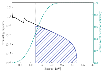
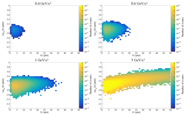
Figure 4.9: Illustration of the DM-nucleus scattering event rate from the Migdal effect with a heavy scalar mediator (solid black line) for $m_{\chi}=0.4\,\mathrm{GeV/c^{2}}$ at $\sigma=1\times 10^{-35}\,\mathrm{cm^{2}}$. Also shown is the efficiency from the in situ tritium measurements performed by the LUX detector (dashed teal line) and the event rate considered for this analysis (hatched blue area) with tritium efficiency and a 1.24 keV energy threshold (dotted gray line) applied.

Figure 4.10: The expected signal from DM-nucleus interactions through Migdal effect at $\sigma=1\times 10^{-35}\,\mathrm{cm^{2}}$ projected onto a two-dimensional space of log₁₀S2 as a function of S1 for four different DM masses. Additional data quality cuts and detector efficiencies were applied. Events in S1 bin smaller than 1 are omitted in the analysis.

The expected event rate for a $1\,\mathrm{GeV/c^{2}}$ DM particle, the detector ER efficiency, and the low-energy cutoff are illustrated in Figure 4.10. The resulting signal model is projected on the two-dimensional space of S1-log₁₀S2 with all analysis cuts applied as shown in Figure 4.10 for various DM masses. S1 pulses are required to have at least a two-PMT coincidence and be in the range of 1-50 phd. Since both S1 and S2 pulses are corrected for geometrical effects, S1 can have values below 2.0 phd even when the two-fold photon coincidence is satisfied.

Figure 4.11 shows the total number of events expected from Bremsstrahlung and Migdal effects without any analysis cuts applied, along with the number of events with only an S2 signal and the total number of events passing all cuts used in the analysis.

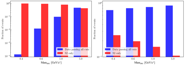
Figure 4.11: The number of events passing all cuts used in the analysis (blue) expected from Bremsstrahlung (left) and Migdal (right). Also shown is the total number of events resulting in an S2-only signal (red). Each plot was normalized to the number of events without any analysis cuts applied.

4.3.2 Background model

The background model used in this work is identical to that used in [187]. An important distinction between [187] and this work is that the sub-GeV signal from both the Bremsstrahlung and the Migdal effects would result in additional events within the ER classification, as identified by the ratio of S2 to S1 size. Whereas the standard WIMP search looks for events in the NR band and is essentially background-free, only dominated by a small leakage of ER events, the sub-GeV signal from these effects sees all ER events as background. The ER band is populated significantly, with contributions from $\gamma$ rays and beta particles from radioactive contaminations within the xenon, detector instrumentation, and external environmental sources as described in [232] and discussed in Section 2.3. Systematic uncertainties in background rates are treated via nuisance parameters in the likelihood; these constraints are listed in Table 4.1.

Parameter	Constraint	Fit value
Low-$z$- origin $\gamma$ counts	$172\pm 74$	$165\pm 16$
Other $\gamma$ counts	$247\pm 106$	$228\pm 19$
$\beta$ counts	$55\pm 22$	$84\pm 15$
127Xe counts	$91\pm 27$	$78\pm 12$
37Ar counts	N/A	$12\pm 8$
Wall counts	$24\pm 7$	$22\pm 4$

Table 4.1: Nuisance parameters in the WS2013 re-analysis likelihood model. Constraints are Gaussian with means and standard deviations indicated. Event counts are after cuts and analysis thresholds. The best-fit model has zero contribution from the signal PDF. In this case, the signal-model parameters float to the central values of their constraints, and so are not listed. Table from [187].

4.3.3 Light yield variation

Systematic uncertainties on the limit from light yield have been studied but were not included in the final profile likelihood ratio (PLR) statistic since their effects were negligible. The impact of $g_{1}$ variation on efficiency is illustrated in Figure 4.13. For the tests, $g_{1}$ was varied by $\pm 20\%$ at three different masses resulting in 9% difference at $0.5\,\mathrm{GeV/c^{2}}$, 6% difference at $1\,\mathrm{GeV/c^{2}}$, and 1% difference at $5\,\mathrm{GeV/c^{2}}$. This is because changing the light yield only affects a small fraction of events passing all analysis cuts due to the applied energy cutoff. The effect on the final limit is illustrated in Figure 4.13. It should be noted that 20% variation was chosen as a case study, but $g_{1}$ is expected to vary by less than 20% in the analysis as the error on light yield obtained from the tritium measurements ranges from 15% at the 1.24 keV threshold to sub-1% at higher energies.

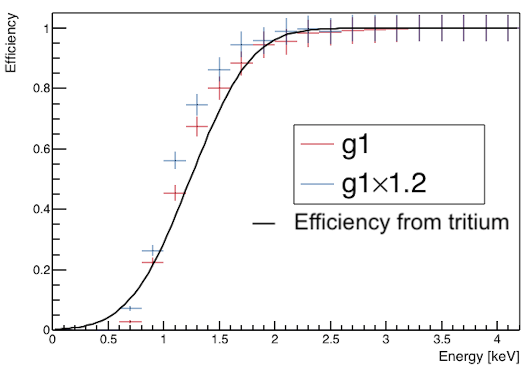
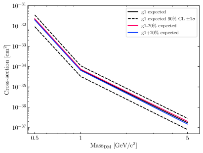
Figure 4.12: Effects of varying $g_{1}$ using NEST v2.0 compared to the efficiency fit from LUX tritium data (black line). Nominal $g_{1}=0.117\,\mathrm{phd}$ per photon is shown in red while the efficiency resulting from a $g_{1}$ increase by 20% is shown in blue.

Figure 4.13: Effects of varying $g_{1}$ for the case of a heavy scalar mediator considering Bremsstrahlung signal model. The expected upper limit on the spin-independent DM-nucleon cross section at 90% C.L with nominal $g_{1}=0.117\,\mathrm{phd}$ per photon is shown in black with the $1\sigma$ range of background-only trials shown in dashed black. The expected limit while varying $g_{1}$ by +20% is shown in pink and by -20% is shown in blue.

4.4 Results

The sub-GeV dark matter signal hypotheses were tested with a double-sided PLR statistic described in Section 2.4.1, scanning over spin-independent DM-nucleon cross section at each DM mass. For each DM mass, a scan was performed over cross sections to construct a 90% confidence interval, with the test statistic distribution evaluated by Monte Carlo sampling using the RooStats package [289]. For an illustration of the expected location of the signal in the S1-log₁₀S2 detector space, contours for various DM masses with different mediators in the case of the Migdal effect are overlaid on the observed events from WS2013 shown in Figure 4.14.

Upper limits on cross section for DM masses from $0.4-5\,\mathrm{GeV/c^{2}}$ for both Bremsstrahlung and Migdal effect assuming both a light and a heavy scalar mediator are shown in Figure 4.15. Upper limits for a light and a heavy vector mediator for the Migdal effect only are shown in Figure 4.16. The observed events are consistent with the expectation from background only.

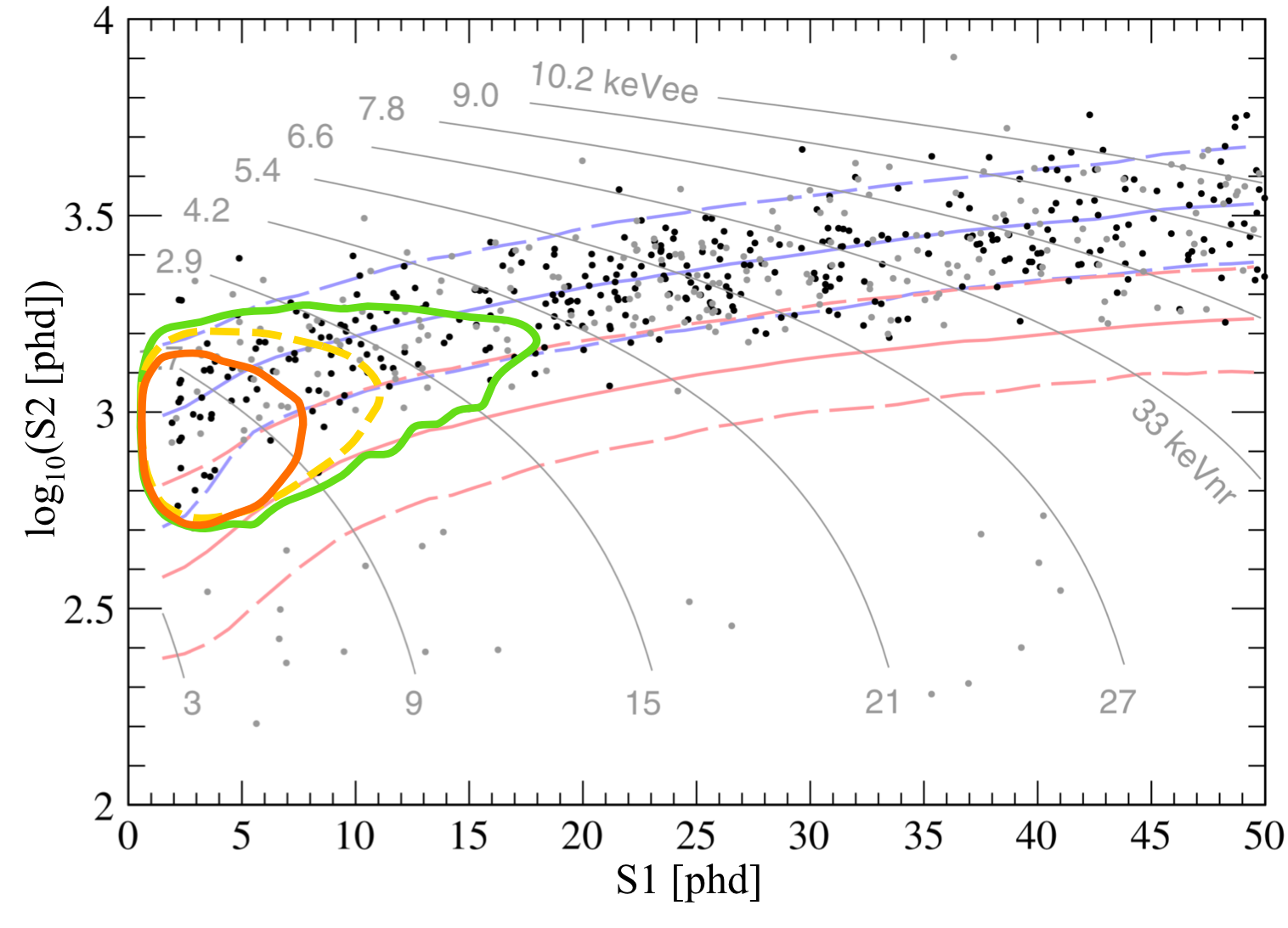
Figure 4.14: Contours containing 95% of expected DM signal from the Migdal effect. The solid contours are for a light vector mediator for $m_{\chi}=0.4\,\mathrm{GeV/c^{2}}$ (light blue) and $m_{\chi}=5\,\mathrm{GeV/c^{2}}$ (teal). Dashed yellow contour assumes a heavy vector mediator and $m_{\chi}=1\,\mathrm{GeV/c^{2}}$. The contours are overlaid on 591 events observed in the region of interest from the 2013 LUX exposure of 95 live days and 145 kg fiducial mass (cf. Reference [187]). Points at <18 cm radius are black; those at 18-20 cm are gray since they are more likely to be caused by background events near the detector walls. Distributions of uniform-in-energy electron recoils (blue) and an example $50\,\mathrm{GeV/c^{2}}$ WIMP signal (red) are indicated by 50^th (solid), 10^th, and 90^th (dashed) percentiles of S2 at given S1. Gray lines, with ER scale of keVee at the top and Lindhard model NR scale of keVnr at the bottom, are contours of the linear-combined S1-and-S2 energy estimator [290].

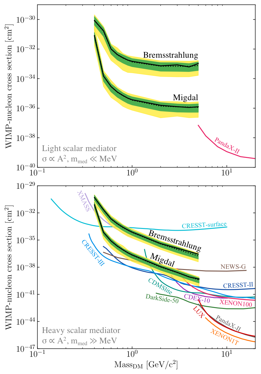
Figure 4.15: Upper limits on the spin-independent DM-nucleon cross section at 90% C.L. as calculated using Bremsstrahlung and Migdal effect signal models assuming a scalar mediator (coupling proportional to mass). The 1- and 2-$\sigma$ ranges of background-only trials for this result are shown in green and yellow, respectively, with the median limit shown as a black dashed line. The top figure shows limit for a light mediator with $q_{\mathrm{ref}}=1\,\mathrm{MeV}$. Also shown is a limit from PandaX-II [291] (pink). The bottom figure shows limits for a heavy mediator along with limits from the spin-independent analyses of LUX [127] (red), PandaX-II [102] (gray), XENON1T [103] (orange), XENON100 S2-only [281] (pink), CDEX-10 [152] (purple), CDMSlite [119] (teal), CRESST-II [121] (dark blue), CRESST-III [122] (light blue), CRESST-surface [123] (cyan), DarkSide-50 [153] (green), NEWS-G [146] (brown), and XMASS [107] (lavender).

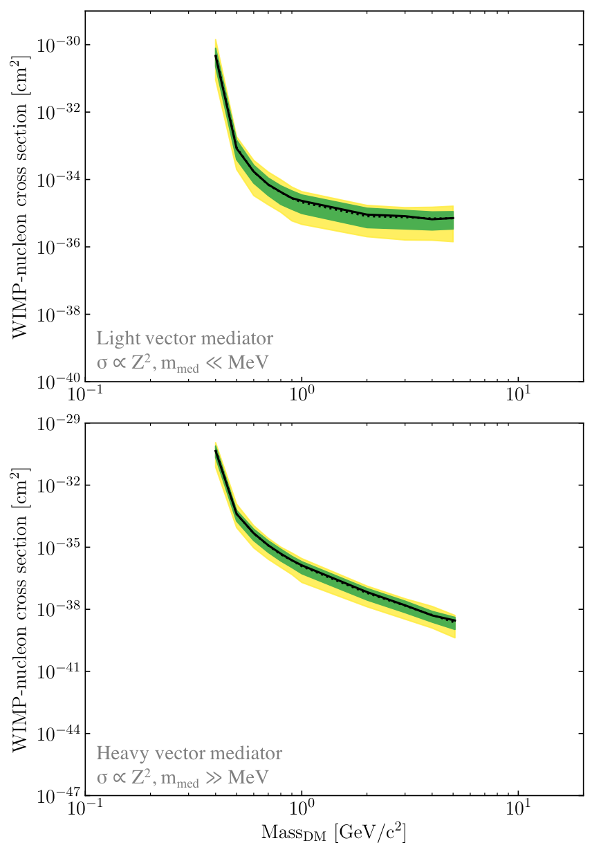
Figure 4.16: Upper limits on the spin-independent DM-nucleon cross section at 90% C.L. as calculated using the Migdal effect signal model assuming a vector mediator (coupling proportional to charge). The 1- and 2-$\sigma$ ranges of background-only trials for this result are shown in green and yellow, respectively, with the median limit shown as a black dashed line. The top figure shows limit for a light vector mediator with $q_{\mathrm{ref}}=1\,\mathrm{MeV}$. The bottom figure shows limit for a heavy vector mediator.

4.4.1 Comments

It should be noted that Bremsstrahlung and Migdal effects are anticipated to be present in the DD calibration data (see Section 2.2.6.3), but have not yet been observed. Even if observed, Bremsstrahlung and Migdal effects would not be recognizable from each other in the analysis, and in fact, the Migdal effect is expected to dominate due to its higher scattering rates. In the current analysis, the electronic energy injections from Bremsstrahlung and Migdal effects likely enhance the S1-log₁₀S2 ratio of the NR signal that dominates. However, these effects are taken into account by the detector NR calibration for a given momentum transfer.

For a detector with a lower NR detection threshold, an analysis could place a limit considering contributions from both NR from elastic scattering and the ER signals presented here. In that case, care should be taken to avoid double-counting of signals.

Note that the Migdal effect can also be used in the future to detect coherent neutrino-nucleus scattering (C$\nu$NS) both from pp and ⁸B solar neutrinos, where the signal is otherwise below threshold (cf. Figure 6 in [283]).

4.5 Conclusion

The contributions from the Bremsstrahlung and Migdal effects extend the sensitivity of the LUX detector to light DM masses previously inaccessible via the elastic nuclear recoil detection method alone. At low DM masses, the recoil signal from the Bremsstrahlung photon and the electrons from Migdal effect is stronger and at higher energies than the elastic NR scattering signal. The presence of these signals in the ER channel is significant because LUX has a higher ER detection efficiency at low recoil energies. Additionally, this search extends the reach of LUX by an order of magnitude in mass without any changes to the detector hardware and sets the first limits on the vector mediator model among direct detection experiments.

This analysis places limits on spin-independent DM-nucleon scattering cross sections assuming both scalar and vector, and light and heavy mediators to DM masses of $0.4\,\mathrm{GeV/c^{2}}$ from $5\,\mathrm{GeV/c^{2}}$. The final limits achieved using the Migdal effect are competitive with limits from detectors dedicated to searches of light dark matter. The observations from LUX are consistent with background only. Nevertheless, this analysis is readily applicable to the next-generation DM detectors, such as LZ [104], by extending the DM search to sub-GeV masses.

Chapter 5 High voltage development for the LZ experiment

The LUX-ZEPLIN (LZ) experiment, a successor to the LUX detector, is a next-generation xenon TPC that will be used to search for dark matter. As noble liquid detectors grow larger in size, new design challenges arise, one of the most prominent being the higher cathode voltage needed to reach the desired drift field. The next two chapters focus on topics associated with high voltage and electric fields in these detectors. In particular, this chapter discusses high voltage delivery to the cathode of the LZ detector whose design, construction, and tests in liquid argon (LAr) are underway at LBNL. Tests are performed in LAr instead of liquid xenon (LXe) because LAr is inexpensive and can be thrown away after each test, obviating the need for a complex and expensive xenon gas handling system. Chapter 6 describes the development, construction, and results from the Xenon Breakdown Apparatus (XeBrA) designed to characterize the breakdown behavior in LAr and LXe.

Since the purity of LAr affects dielectric breakdown behavior, it is essential to provide a purity measurement in these tests. To that end, I designed and built a compact purity monitor. The purity monitor is a small double-gridded drift chamber fully submerged in LAr. Electrons are extracted from a photocathode via photoelectric effect, and LAr purity is measured as a function of the number of electrons that attach to impurities. The purity monitor can be operated at a wide range of electric fields which allows this purity monitor with a total length of 7 cm to measure electron lifetimes of up to 1 ms.

This chapter first provides a brief overview of the LZ experiment (Section 5.1), the challenges of HV design in two-phase TPCs (Section 5.1.2), and the development of the HV connection for the LZ detector (Section 5.1.3). The second part of this chapter focuses on the design and operating principles of liquid noble purity monitors (Section 5.3). After the successful construction and testing of the purity monitor for LZ (Section 5.3.2), a second purity monitor was developed for the XeBrA experiment (Section 5.4). Additionally, a third purity monitor is currently under construction, closely following the design of XeBrA’s purity monitor, to be deployed in an experiment studying optical reflectivity of PTFE in liquid xenon.

5.1 The LUX-ZEPLIN experiment

The LUX-ZEPLIN (LZ) experiment was formed by a merger of two collaborations - LUX (discussed in Chapters 2, 3, and 4) and ZEPLIN (ZonEd Proportional scintillation in LIquid Noble gases) [293, 99, 294]. The LZ collaboration consists of $\sim 250$ physicists and engineers from 31 institutions in the USA, UK, Portugal, and South Korea. Its goal is to explore the bulk of the region remaining above the neutrino floor with sensitivities to spin-independent (SI) and spin-dependent (SD) cross sections of $10^{-48}$ $\left(10^{-46}\right)\,\mathrm{cm^{2}}$ for a 40 GeV/c² WIMP mass after an exposure of 1,000 live-days. To achieve that, LZ will feature many upgrades compared to its predecessors: a significantly larger active xenon mass, a powerful nested veto system, new calibration systems, and a rigorous cleanliness program including comprehensive radio-assay and dust reduction programs. This section draws from the recent LZ sensitivity prediction publication [104]; further technical details about LZ design can be found in the Conceptual Design Report from September 2014 [295] and in the Technical Design Report from March 2017 [296].

Similarly to LUX, the LZ detector will operate 1478 m (4850 ft) below ground at the Sanford Underground Research Facility (SURF) in the Davis Cavern, which has undergone many modifications to accommodate the upgrades planned for the LZ detector. The LZ detector will be located inside the water tank inherited from the LUX experiment. The water tank will be filled with 228 tonnes of ultrapure water and instrumented by PMTs surrounded by Tyvek diffuse reflectors to improve light efficiency. As in LUX, the water tank provides shielding from muons, neutrons, and $\gamma$-rays from the naturally occurring radiation in the cavern rock and the PMTs.

The LZ detector will be housed inside outer and inner cryostats made from titanium with some of the lowest ever reported intrinsic activities [297]. The TPC is cylindrical with both height and diameter equal to 1.46 m as shown in Figure 5.1. The 7 tonnes of active xenon are viewed by 494 PMTs: 241 at the bottom and 253 at the top. The active volume is surrounded by segmented, cylindrical, and highly reflective PTFE panels that embed 57 field shaping rings. The xenon circulation and purification strategies are based on the LUX system.

One of the most notable LZ detector upgrades compared to the LUX detector is the improved veto system. First, the active volume of the TPC is surrounded by a xenon skin region illustrated in Figure 5.2 of a zoomed image of the cathode region. The xenon skin region is composed of the outermost 2 tonnes of LXe located between the outside of the PTFE panels and the inner titanium cryostat. The titanium walls are lined with a thin layer of PTFE to improve light collection. The xenon skin region is optically isolated from the main active volume and is instrumented by PMTs. The xenon skin maximizes the use of LXe inside the detector and helps reject scattered $\gamma$ rays that could contribute to the backgrounds.

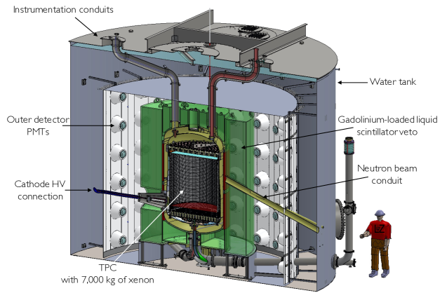
Figure 5.1: A cutaway of a CAD rendering of the LZ detector. PMT and other cables from the bottom of the TPC exit through a port at the bottom of the cryostat. Figure modified from [104].

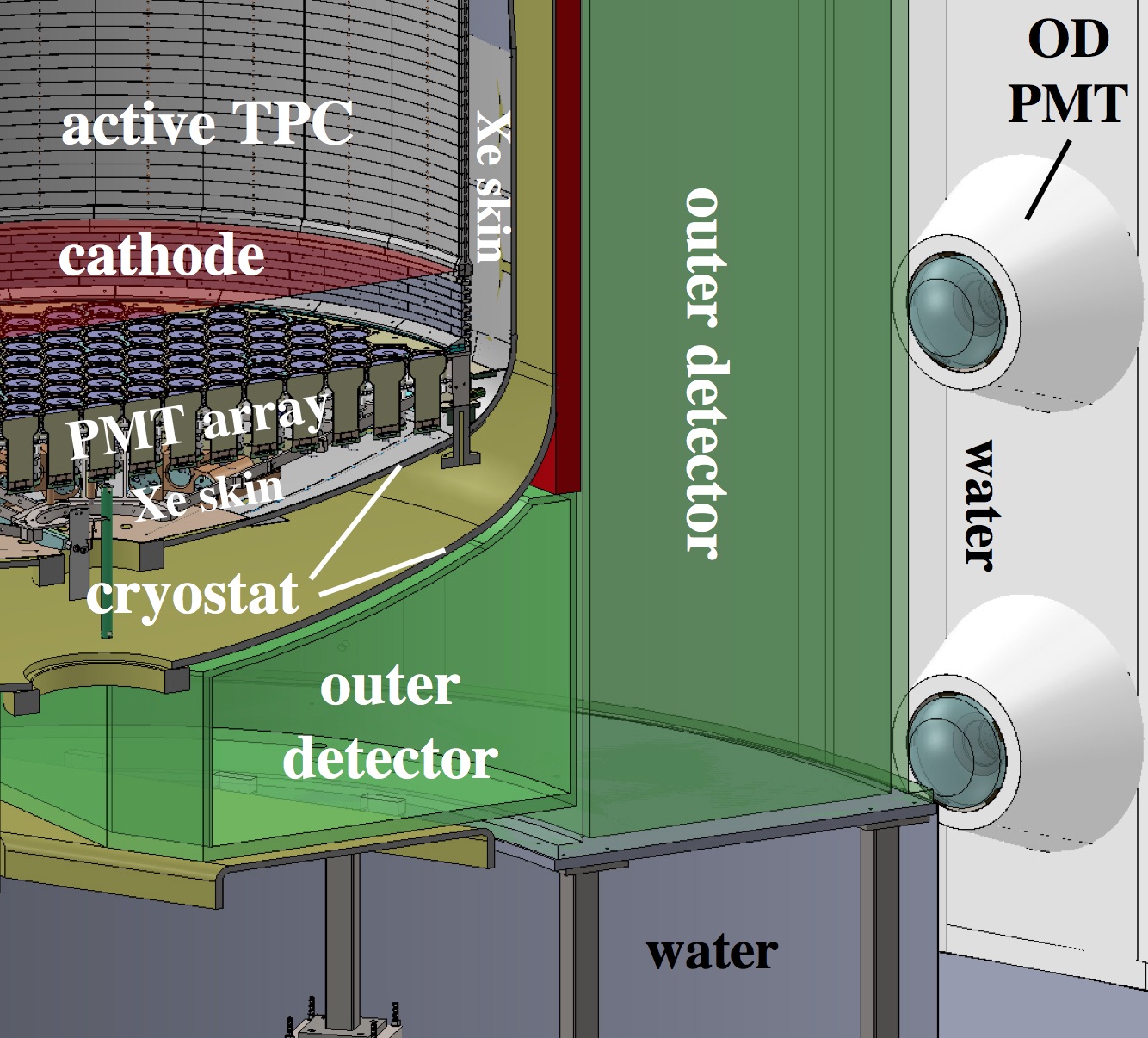
Figure 5.2: An expanded view of the lower right corner of the LZ cathode region. ‘OD PMT’ indicates the outer detector photomultiplier tubes. The xenon skin region is observed by an independent set of PMTs not depicted. Figure from [104].

The second veto component consists of 17 tonnes of gadolinium-loaded liquid scintillator (GdLS) contained in 10 acrylic tanks viewed by the PMTs inside the water tank. The GdLS veto is located just outside the outer cryostat as depicted in green in Figures 5.1 and 5.2. Its principal goal is to detect neutrons from $\left(\alpha,n\right)$ processes since single scatter neutrons represent the most dangerous background for WIMP searches. If such a neutron single scatters inside the TPC, the neutron will be thermalized and captured within $\sim 30\,\mathrm{\mu s}$ in the GdLS. The Gd neutron capture results in $\sim 8\,\mathrm{MeV}$ of $\gamma$ ray cascade, which can be detected by the skin or the water tank PMTs, thus vetoing the event. The efficiency of this process to identify a neutron that produces a single scatter event in LXe above the analysis threshold is 96.5% [104, 298]. The entire veto system also makes possible an extended fiducial volume cut as illustrated in Figure 5.3. Selected parameters of the LZ detector are summarized in Table 5.1.

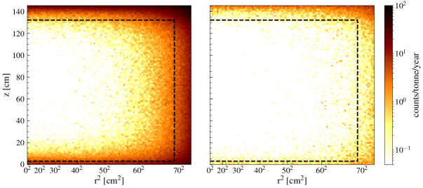
Figure 5.3: Single scatter event distribution from all NR backgrounds in the region of interest for a $40\,\mathrm{GeV/c^{2}}$ WIMP. The black dashed line illustrates a 5.6 tonnes fiducial volume. Left: Event distribution with no veto results in 12.31 counts/1,000 days. Right: Only 1.03 counts/1,000 days remain after applying both xenon skin and GdLS vetoes. Figure modified from [104].

Category	Parameter	Value	Note
Liquid xenon	Total mass	9,600 kg
	TPC active mass	7,000 kg
	Skin mass	2,000 kg
	Fiducial mass	5,600 kg
PMTs (all from Hamamatsu)	TPC	253 (top) +
241 (bottom)	3” R11410-22
	Side skin (top)	93	1” R8520
	Side skin (bottom)	20	2” R8778
	Dome skin	18	2” R8778
	Water tank	120	8” R5912
TPC dimensions (cold)	Inner cryostat diameter	1.58-1.66 m
	Inner cryostat height	1.83 m
	Skin thickness	40 mm (surface),
80 mm (cathode)
	TPC diameter	1,456 mm
	Gate-anode	13 mm
	Cathode-gate	1,456 mm
	Bottom PMT-cathode	137.5 mm
	Field cage thickness	15 mm
Electric fields	Extraction region	10.2 kV/cm
	Drift field	343 V/cm (baseline)	686 V/cm (goal)
	Reverse field	2.9 kV/cm (baseline)	5.9 kV/cm (goal)
Operations	Electron lifetime	850 $\mu$s	Lower limit
	Pressure	1.8 bar	Pressure range
1.6 - 2.2 bar
	Equilibrium temperature	175 K

Table 5.1: Summary of key characteristics of the LZ detector. The inner cryostat has a tapered radial profile in order to lower the magnitude of electric fields around the cathode region near the bottom of the detector. The “Note” column includes the diameter and model information of the various PMT types used in the detector.

LZ will build on the extensive calibration experience from the LUX detector, but its much larger size requires the development of additional calibration methods. The goal of LZ is to detect WIMP-nucleus interactions in LXe. To separate those events from background, it is imperative to characterize the detector response to nuclear (NR) and electron recoils (ER). This can be achieved through calibrations. Several internal and external sources will be used for ER calibrations of the LXe response:

• Along with $\mathrm{{}^{83m}Kr}$ $\left(41.5\,\mathrm{keV}\right)$ that was also used in LUX as described in Section 2.2.6.1, LZ will also use $\mathrm{{}^{131m}Xe}$ produced via decay of $\mathrm{{}^{131}I}$. The $\mathrm{{}^{131m}Xe}$ nucleus decays into $\mathrm{{}^{131}Xe}$ by emitting a $\gamma$ with 163.9 keV and a half-life of 12 days.

• ³H ($\beta$ decay with Q $=18.6\,\mathrm{keV}$) and ¹⁴C internal calibrations are also planned at several milestones throughout data taking to provide a thorough mapping of ER light and charge yields. Similarly to the tritium source, ¹⁴C will be injected as ¹⁴C-labeled methane (¹⁴CH₄). It transitions to ¹⁴N via a beta decay with 5,730 year half-life and $Q=156\,\mathrm{keV}$. This calibration was tested after the end of LUX dark matter search and is described in [199].

• ${}^{228}\mathrm{Th}$ will be used to calibrate signal fidelity near the edge of the TPC. ${}^{228}\mathrm{Th}$ is part of the thorium series, which ends when ²⁰⁸Tl undergoes a beta decay with a half-life of 3.1 minutes into ²⁰⁸Pb followed by a 2,615 keV $\gamma$ with 99.8% branching fraction. External sources will be deployed in 3 vertical stainless steel calibration tubes located in the vacuum space between the inner and outer titanium cryostats.

Similarly, various external calibrations are planned to measure detector NR yields in LXe.

• A DD (2,450 keV) generator, used in LUX and described in Section 2.2.6.3, will be used again.

• AmBe (maximum neutron energy of 11 MeV) and AmLi sources will be deployed in the external calibration tubes. The AmLi source is preferable over AmBe (that was used in LUX) due to its lower maximum neutron energy of 1.5 MeV, resulting in an enhanced fraction of events at low recoil energy of <10 keV.

• Additionally, photoneutron sources with well-defined kinematic endpoints are being developed to calibrate low-energy NR and coherent scatters from ⁸B neutrinos. One such photoneutron source is ⁸⁸YBe, which produces 1.836 MeV $\gamma$ along with 152 keV neutrons [299], resulting in an NR endpoint of $4.6\,\mathrm{keV}$. Several other photoneutron sources are being considered as well. They will be deployed on-axis on top of the outer cryostat vessel reaching just above the inner cryostat.

Furthermore, ${}^{220}\mathrm{Rn}$ will be used for xenon skin calibrations, and separate calibrations are planned for the GdLS outer detector. However, the calibration plan will likely change and evolve as the needs of the detector become better known.

LZ will use a simulation framework called BACCARAT based on the Geant4-based LUXSim package. The anticipated amount of background events for LZ is being carefully tracked and a table with an overview of estimated backgrounds can be found in [104]. Figure 5.4 shows the spectral contribution for ER and NR backgrounds in the fiducial volume. As can be seen, radon presents the largest contribution to the total number of background events, while atmospheric neutrinos present the most significant contribution to NR counts. The expected number of total background events after all cuts is 5.97 counts of ER and 0.52 counts of NR in the region of interest.

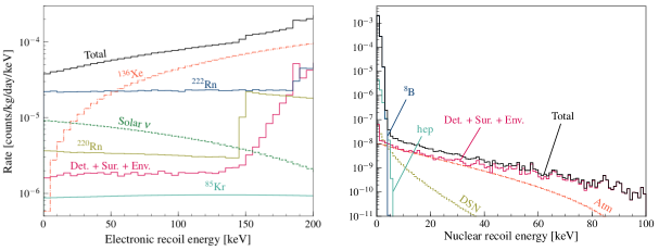
Figure 5.4: Background spectra in the 5.6 tonne fiducial volume for single scatter events with neither a xenon skin nor a GdLS veto signal. No detector efficiency or WIMP-search region cuts have been applied. Left: ER. Right: NR. Figures from [104].

Similarly to LUX, LZ will employ salting to prevent analysis biases, and once the final dataset is established, PLR will be used to set a limit. There are eleven types of background considered as nuisance parameters in the PLR code. Figure 5.5 shows the separation of the ER and NR bands with simulated 1,000 live-days of background-only data and the expected limit if a WIMP signal is not observed.

Figure 5.5: Expected results from 1,000 live-days with 5.6 tonne fiducial mass. Left: LZ background-only simulated dataset. The mean (solid) and the 10 and 90% contours (dashed) indicate the NR (red) and ER (blue) bands. Also shown (yellow shaded) are 1- and 2-$\sigma$ regions for an expected $40\,\mathrm{GeV/c^{2}}$ WIMP signal and ⁸B and $hep$ NR backgrounds (purple contours). Right: LZ projected sensitivity to SI WIMP-nucleon elastic scattering for 1,000 live-days and a 5.6 tonne fiducial mass. The lower shaded region bounded by the red dashed line indicate the emergence of backgrounds from neutrino coherent scattering [300, 237]. Gray contoured areas show the favored regions from pMSSM11 [159]. Figures from [104].

5.1.1 Modeling electric fields in the LZ detector

The electric fields inside the TPC are set by the field shaping rings built at LBNL and four mesh grids weaved on a custom-built loom at SLAC National Accelerator Laboratory (SLAC). The grid parameters are summarized in Table 5.2.

Grid	$z$ [cm]	Wire$\,\diameter$ [$\mu$m]	Pitch [mm]	Operating voltage [kV]
Anode	161.65	100	2.5	5.75
Gate	160.35	75	5.0	-5.75
Cathode	14.75	100	5.0	-50.00
Bottom shield	1.00	75	5.0	-1.50

Table 5.2: Grid properties and voltages as designed for the LZ detector. All grids are wire meshes woven from 304 stainless steel from California Fine Wire company. A linear voltage grading is established by a series of resistors between cathode and gate. The face of the bottom PMT array is defined at $z=0$. The liquid level is assumed to be 5 mm above the gate grid.

Building a full 3D model of the detector, as was done for the LUX detector (Chapter 3), is not simple and is not always necessary. Most often, a much simpler, axially symmetric model will suffice to improve understanding the behavior of electric fields inside a detector’s active volume. However, most TPCs contain grids with either parallel or mesh wires, which break axial symmetry. It is essential to understand the transformation of the detector geometry and its grids between a full 3D model and an axially symmetric model to account for these changes since as was shown in Figure 3.7, grid transparency has a substantial effect on field leakage and therefore on the electric fields in the detector’s active volume. The study below was conducted to inform the field modeling efforts of the LZ experiment.

5.1.1.1 Effects of modeling field grids in axially symmetric geometry

Often optical transparency, defined as 1-diameter/pitch, is taken as a proxy for electrostatic transparency, but as will be shown this is not always a sound assumption. Therefore a study was conducted to investigate the effects of various grid geometries on electrostatic transparency. A simple 3D model was created in COMSOL Multiphysics of a cylinder filled with LXe with dielectric constant $\varepsilon=1.85$ with a plane at the bottom with $V_{\mathrm{bottom}}=-1.5\,\mathrm{kV}$ at $z=0\,\mathrm{cm}$, a grid at $z=13.7\,\mathrm{cm}$ with $V_{\mathrm{cathode}}=-50\,\mathrm{kV}$, and a plane on top at $z=26.9\,\mathrm{cm}$ with $V_{\mathrm{top}}=-46\,\mathrm{kV}$ corresponding to a field of $303\,\mathrm{V/cm}$ in the active volume. Zero-charge boundary $n\cdot D=0$ was imposed around the edges of the model. This mimics the settings in the center of the LZ detector described in Section 5.1. Three different grid geometries were modeled as illustrated in Figure 5.6 each with the same grid diameter $d_{1}=100\,\mathrm{\mu m}$ but with a varying pitch: a parallel wire grid with pitch $p_{1}=2.5\,\mathrm{mm}$, a mesh wire grid with pitch $2\cdot p_{1}$, similar to the one used in LZ, and a grid consisting of concentric rings of wires with pitch $p_{1}$. The last geometry corresponds to the transformation of a parallel wire grid into the solution of an axially symmetric model.

These three geometries were chosen because the goal of these studies was to determine whether an axially symmetric simulation would suffice for investigations of electric fields inside the active volume of the LZ detector. As LZ uses a mesh grid, representing that in an axially symmetric model requires first to approximate the mesh grid as a parallel grid (which is done by doubling the pitch) and then it is necessary to investigate how the parallel grid compares to the concentric wire grid modeled in the axially symmetric simulation.

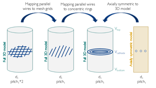
Figure 5.6: Illustration of different geometries modeled to study grid transparency effects.

Each of the three geometries was solved with the same boundary conditions and the resulting fields were compared. A 2D figure illustrating the field difference between the mesh and parallel wire geometry and between the parallel and concentric wire geometry is shown in Figure 5.7. The field leakage in the active volume differs between the different grid geometries, but appears to be $<2\%$ at $\sim 1\,\mathrm{cm}$ away from the grids. Despite this small difference, due to the increase in computational complexity for a full 3D model, the axially symmetric models appear to be reasonable approximations. It should be noted that the grid transparency increases with increasing radius so the field leakage will be most pronounced at high radius close to detector edges.

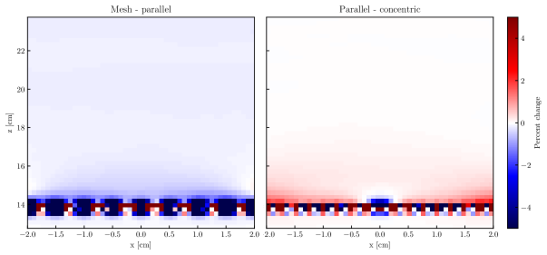
Figure 5.7: A 2D figure illustrating the field leakage difference between a mesh and a parallel wire geometry (left) and a parallel and a concentric wire geometry (right). Only a small $<2\%$ difference further than $\sim 1\,\mathrm{cm}$ away from the grids is visible.

5.1.1.2 Understanding field leakage as a function of grid geometry

A brief study using the well understood LUX axially symmetric model was undertaken to visualize the effects of varying grid geometries on grid transparency and the resulting field leakage. As shown in Figure 5.8 the same optical transparency stemming from various wire diameters and pitches (visible along the diagonal) results in wildly varying electric fields inside the detector’s active volume. This illustrates that optical transparency can be used as a proxy for electrostatic transparency only if the wire diameter and pitch are not excessively modified.

These studies confirmed that an axially symmetric simulation with wire diameter and pitches that respect the observations described here are appropriate for the initial electric field model of the LZ detector.

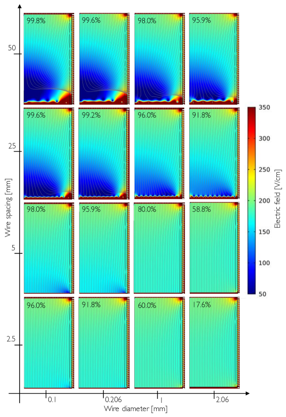
Figure 5.8: The wire diameters and pitch of the baseline axially symmetric model used for visualization in WS2013 shown at $\left(0.206,\,5\right)$ was modified to illustrate effects of grid geometries on field leakage. Optical transparency of each model is indicated in its upper left corner and is defined as 1-diameter/pitch. The model at $\left(0.1,\,2.5\right)$ mimics the grid transparency of the LZ detector model described in Section 5.1.1.

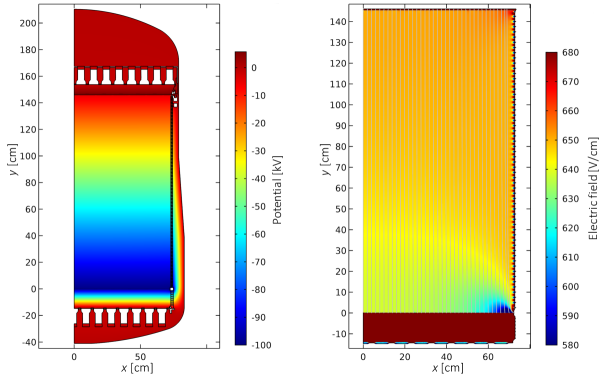
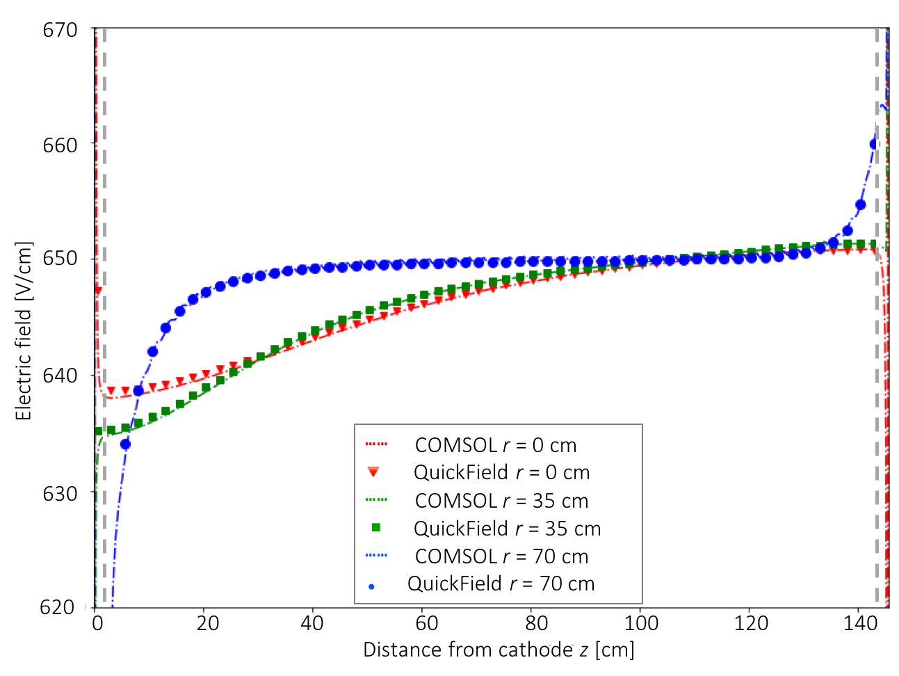
Figure 5.9: Model of the LZ detector with a cathode voltage of -100 kV. Left: Potential in the LZ detector. The region with one of the highest fields in the detector can be seen between the cathode and the bottom shield grids (here between $y\sim-15-0\,\mathrm{cm}$). It is referred to as reverse field region since the electric field direction is opposite to the active volume. Right: Active volume of the LZ detector with field lines shown in gray. The low and high field pockets also seen in the LUX model (see Figure 3.7) are present as expected.

Figure 5.10: Comparison of the LZ electric fields as obtained from COMSOL and QuickField models at three different vertical distances from the detector center. The gray dashed lines indicate the drift time fiducial volume boundary. The slight discrepancy at the low and high $z$ is due to meshing anomalies in the QuickField simulation.

5.1.1.3 The LZ field model

I built an axially-symmetric model in COMSOL Multiphysics that served as an independent check for the electric field optimization studies done by Reed Watson using the QuickField simulation package [301]. The resulting model is shown in Figure 5.10 and presents good agreement with simulations done in QuickField as illustrated in Figure 5.10.

5.1.2 Hardship of high voltage in two-phase TPCs

A two-phase TPC works by detecting light and charge generated during interactions in the active detector material. In order to detect the charge generated by an interaction, the electric field needs to be present to transport the charge to its detection site. In LUX and LZ, the charge is detected by creating a secondary scintillation signal via electroluminescence in xenon gas, but other methods can be used as well. Generally, an electric field of $\mathcal{O}\left(100-1,000\right)$ V/cm in the bulk of LXe is required to achieve acceptable S2/S1 discrimination and prevent event pile-up in the detector. Therefore, with the increasing length of the drift region, it is necessary to deliver increasingly higher voltages to achieve adequate electric field inside the active volume. By design, in two-phase TPCs the cathode is biased at a negative high voltage to enable electrons to drift toward the liquid-gas interface where the field is further increased to facilitate electroluminescence. Based on the length of the drift region, that means the cathode needs to be biased to voltages $\mathcal{O}\left(10-100\right)$ kV with only a small current needed to supply the TPC grading resistors. However, this has proven to be a challenge in the past.

There are two sets of issues. First, there is the risk of a full dielectric breakdown, which can cause irreparable damage to the detector hardware. Second, there are concerns regarding elevated light production and electron emission from regions with high fields since these typically arise at lower voltages than a complete breakdown. Elevated light production can cause an increased rate of low-energy S1-like signals, while electron emission creates additional S2 signals. These can increase the detector dead time by increasing the event rate and contributing to the loss of WIMP sensitivity. Most commonly, the spurious light and charge emission is caused by grid wires due to their small diameter, but resistors, screws, and edges of miscellaneous parts at HV can cause these too. Furthermore, increased electron emission can cause material degradation, which can result in unexpected failure of a detector part.

There are no commercially available solutions to deliver high voltage from a power supply located in the lab to the cathode of a liquid noble TPC. Therefore, each collaboration develops a customized solution. Ethan Bernard developed both the LUX and the LZ feedthroughs. The development of these high voltage delivery systems is discussed in [193]. The design goal for the LUX HV feedthrough was -100 kV. The feedthrough was successfully tested at that voltage in oil at Yale University. However, the LUX cathode was never biased to that voltage during operations due to the onset of light emission in the detector at lower voltages. Instead, the detector operated at -10 kV and -8.5 kV during WS2013 and WS2014-16, respectively. Unfortunately, this is not unusual; other detectors faced similar pains and were forced to operate at lower fields than designed, usually due to the appearance of small light pulses. The design goals and broken high voltage dreams of several collaborations are summarized in Table 5.3.

Detector	Drift length [cm]	Drift field [V/cm]	Operating HV [kV]	Design HV [kV]
ZEPLIN-III [294, 99]	3.5	3,400	-12.0	-35
XENON10 [302]	15.0	730	-13.0	N/A
XENON100 [303]	30.5	530	-16.0	-30
LUX [187, 163]	48.0	50-600	-8.5	-100
Panda-X II [304, 102]	60.0	318	-24.0	-36
XENON1T [103, 155]	97.0	81	-8.0	-97
LZ (projected) [104]	146.0	310	-50.0	-100

Table 5.3: Design goals and realities of two-phase TPC HV. The operating voltages are reported from each detector’s latest scientific runs. The design HV refers to either the projected performance or the highest reported value from TPC tests in the commissioning phases as available. Table adapted from [305].

In order to avoid the high voltage hardship experienced by the previous generations of LXe dark matter experiments, LZ has invested much effort into the development and testing of its high voltage systems. The wires were tested at Imperial College London [306], several tests of grids are being conducted at SLAC, and the cathode HV feedthrough development started at Yale University and continued at LBNL as discussed in the next section.

5.1.3 LZ high voltage cathode connection

The central goal of high voltage delivery is maintaining cathode at the appropriate voltage. This requires careful management of electric fields around any conductors at high potential, which is particularly intricate when it comes to the termination of the grounding shield of the coaxial cable used for HV delivery. There are several options for high voltage delivery from the power supply to the detector’s cathode. Most simply, conventional HV feedthroughs can be purchased, as was done in the XeBrA detector described in Chapter 6. However, conventional feedthroughs are often made from radioactive materials or are unsuitable for use in cryogenic temperatures. Another option is to avoid the delivery of high voltage altogether by creating it within the detector [307], an option favored by experiments performed in liquid helium where thermal insulation is important [308, 309], but also used in LAr detectors [310]. This solution is not optimal for LZ where it is desirable to maximize the use of the LXe volume for WIMP detection.

The conservative design of the LZ feedthrough features a very careful termination of the coaxial ground shield, which occurs in LXe near the cathode. Because of the geometry, a high field region is unavoidable. Therefore, the goal of the design is to minimize LXe exposure to high fields to prevent spurious breakdowns. A smaller quantity of LXe is preferable because small length-scales, in general, perform better at high fields as will be discussed in great detail in Chapter 6. From there, a linear voltage grading enforces smoother fields in this critical region. Additionally, a leak-tight seal is required between the cable and the cryostat to prevent the introduction of impurities and xenon loss. Various cryogenic detectors face these issues, so the LZ cathode connection design builds on experiences of previous experiments. To learn more about the design and development of both LUX and LZ feedthroughs, consult Reference [193]; this section discusses the testing of the final design of the LZ cathode HV connection.

Because of logistical, spatial, and design considerations, the LZ cathode HV connection is made from the side of the detector as shown in Figure 5.11. In LUX, HV was delivered from the top of the cryostat through the side of the TPC as shown in Figure 2.7. Having the cable come from the top makes the detector construction more straightforward, but creates undesirable high fields within the inner cryostat. If instead, the HV cable arrives to the detector from the side near the cathode it avoids perturbing electric fields inside the TPC. This approach also allows a larger volume of LXe surrounding the cathode connection, increasing distances from HV to ground. In fact, unlike LUX, LZ has no metal parts between the TPC and the inner cryostat walls in an attempt to minimize electric fields in the fiducial volume. For this reason, the LZ cryostat is larger near the bottom, which then makes space for the skin veto.

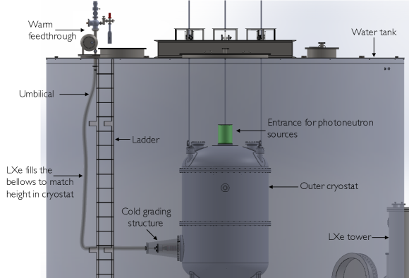
Figure 5.11: Overview of the HV delivery system from the lab to the detector. To thermally insulate xenon from the water tank, a 1” diameter bellows is nested inside a 3” diameter bellows, which is used as a vacuum jacket and will be filled with super-insulation. The inner bellows connects to the xenon space of the inner vessel, and the evacuated outer bellows connects to the vacuum space of the outer cryostat. The vacuum space of the warm feedthrough will be monitored for gas leaks by an RGA.

An uninterrupted length of cable will connect from the LZ cathode power supply installed in the underground lab to the cathode connection region inside the LZ cryostat. LZ uses an all-plastic Dielectric Sciences cable model SK160318 rated up to 150 kV shown in Figure 5.12. There are two points of interest on this path. First, there is a room temperature feedthrough that makes a leak-tight seal between air and xenon. The warm feedthrough features a double O-ring seal with a spool of extra cable needed to allow for thermal contraction of the cable.

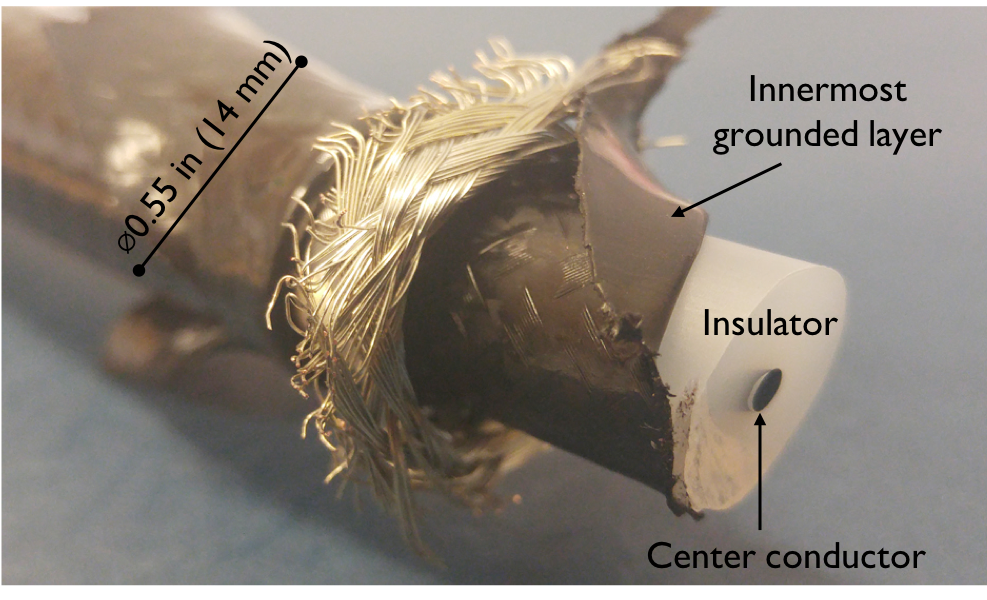
Figure 5.12: Coaxial cable from Dielectric Sciences model SK160318 rated to 150 kV. The insulating layer is made from polyethylene and the innermost grounded layer, and the conductive core are made from semiconductive polyethylene with $\sim 2800\,\mathrm{\nicefrac{{\Omega}}{{ft}}}$. The diameter of the conductor is 0.08 in (2.0 mm), the diameter of the insulating dielectric is 0.44 in (11.2 mm), and the thickness of the grounded layer is 0.01 in (0.3 mm). A single uninterrupted piece of cable ($\sim 30\,\mathrm{m}$) will connect the HV power supply directly to the cathode connection structure.

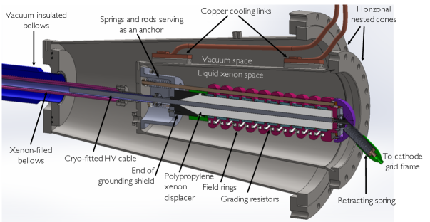
Figure 5.13: CAD rendering of the cold grading structure. The ground of the HV cable is terminated within the stress cone (black) made from conductive plastic. The field shaping rings are made from conductive plastic and are linked together by linearly-graded resistors to taper off the ground connection smoothly. The connection to the cathode frame is made by a retracting spring whose flexibility ensures the connection does not break during thermal cycling.

Second, there is a cold connection near the cathode that provides termination of the ground shield of the cable. Creating a connection between the cathode and the HV delivery system that does not cause excessively high electric fields, is secure, and can sustain thermal cycling is often one of the critical parts of the HV design, due to its complexity. A diagram of the cold connection used in LZ is shown in Figure 5.13. The cable is routed in two bellows (flexible hoses) connecting the warm and cold grading structures to a couple of cones attached to the side of the LZ detector. The outer cone is attached to the outer cryostat that provides thermal insulation to the inner cryostat. The inner cone is connected to the inner cryostat and is filled with LXe. The grounding shield of the HV cable is terminated inside the LXe cone. From there, HV is carefully stepped up from ground to its maximum voltage (purple hemisphere on the right) through a series of field shaping rings with linear voltage grading. The electric field simulation of this region is shown in Figure 5.14. The grading structure accomplishes to keep the electric field below 50 kV/cm in LXe, which is the LZ design specification requirement.

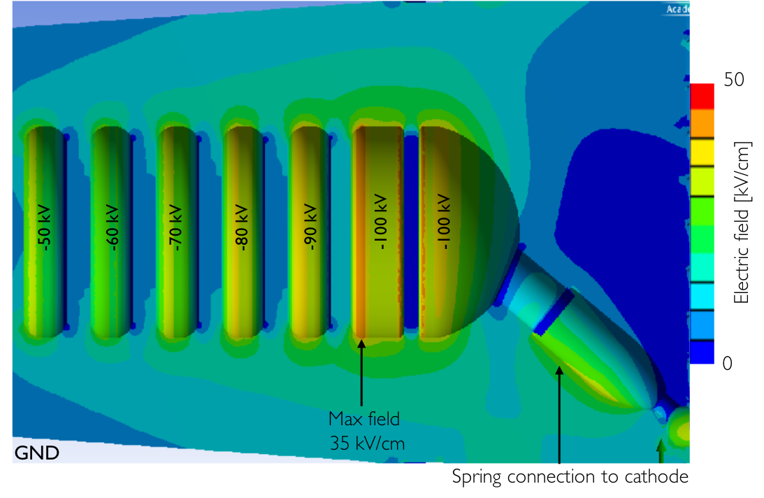
Figure 5.14: A simplified 3D electrostatic simulation of the HV cold grading structure done by Evan Pease in ANSYS Maxwell simulation software [311]. Only the first six field shaping rings are shown. The spring connecting the grading structure to the cathode has been simulated as a cylinder. All the simulated parts have electric fields below 50 kV/cm, with the highest field of 35 kV/cm occurring on the first field shaping ring when -100 kV is applied to the cathode.

The cable itself is cryofitted with polypropylene to exclude xenon from the high field region. The cryofit ensures that the cable and its expander undergo the same thermal contractions preventing xenon leaking into the space. Three springs pull on rods holding the feedthrough to ensure structural rigidity. The field shaping rings are made from conductive plastic and are linked together by resistors that smoothly taper off the ground connection to control electric field along the insulating surface of the cable to prevent breakdown. The connection to the cathode is made with a conductive spring, providing adequate mechanical compliance and straightforward connection during assembly. Additionally, two copper links attached to the HV cone cool the upper surface of the cone below the LXe boiling temperature thus preventing accumulation of bubbles. Xenon bubbles are undesirable because xenon gas has a lower dielectric strength compared to LXe and therefore is more likely to cause a breakdown. Furthermore, the difference in dielectric constants enhances electric fields within the gas. The other ends of the thermal links are connected to a thermosyphon that acts as a heat sink.

5.1.3.1 Feedthrough tests at LBNL

To ensure that the cathode HV feedthrough performance meets design expectations during 10 years of operation, extensive tests of the cold grading structure are being conducted at LBNL. Several cryocycling tests were performed of the HV cable and the xenon displacer cryofit structure. Tests of the design of the grading structure are also underway in the custom-built seismically-anchored HV cage shown in Figure 5.15. Testing is performed in LAr since its HV performance is close to xenon at a fraction of the cost. The test system, therefore, does not require expensive recirculation systems and other infrastructure needed to prevent xenon loss. During the tests, the cone and grading structures are submerged in LAr, and a high voltage is delivered to the structure from the HV power supply located on the top of the blue grounded cage. Discharges are monitored by charge-sensitive amplifiers, a set of cameras, and a PMT located at the bottom of the test structure. Since the 128 nm LAr scintillation light is not visible to the PMT, a tetraphenyl butadiene (TPB)-coated acrylic pane is located in front of it serving as a wavelength shifter. TPB fluoresces promptly and efficiently, re-emitting the light with a peak at 430 nm [312]. A dedicated purity monitor described in Section 5.3 is also installed inside the cryostat since dielectric breakdown depends on the purity of the noble liquid as discussed in Section 5.2. LAr is discarded at the end of each testing cycle. Description of the electrical simulation of the feedthrough is available in [193].

Initial analysis shows that the feedthrough performs within the ranges required for LZ. An upcoming publication about the feedthrough design, testing, and performance is planned.

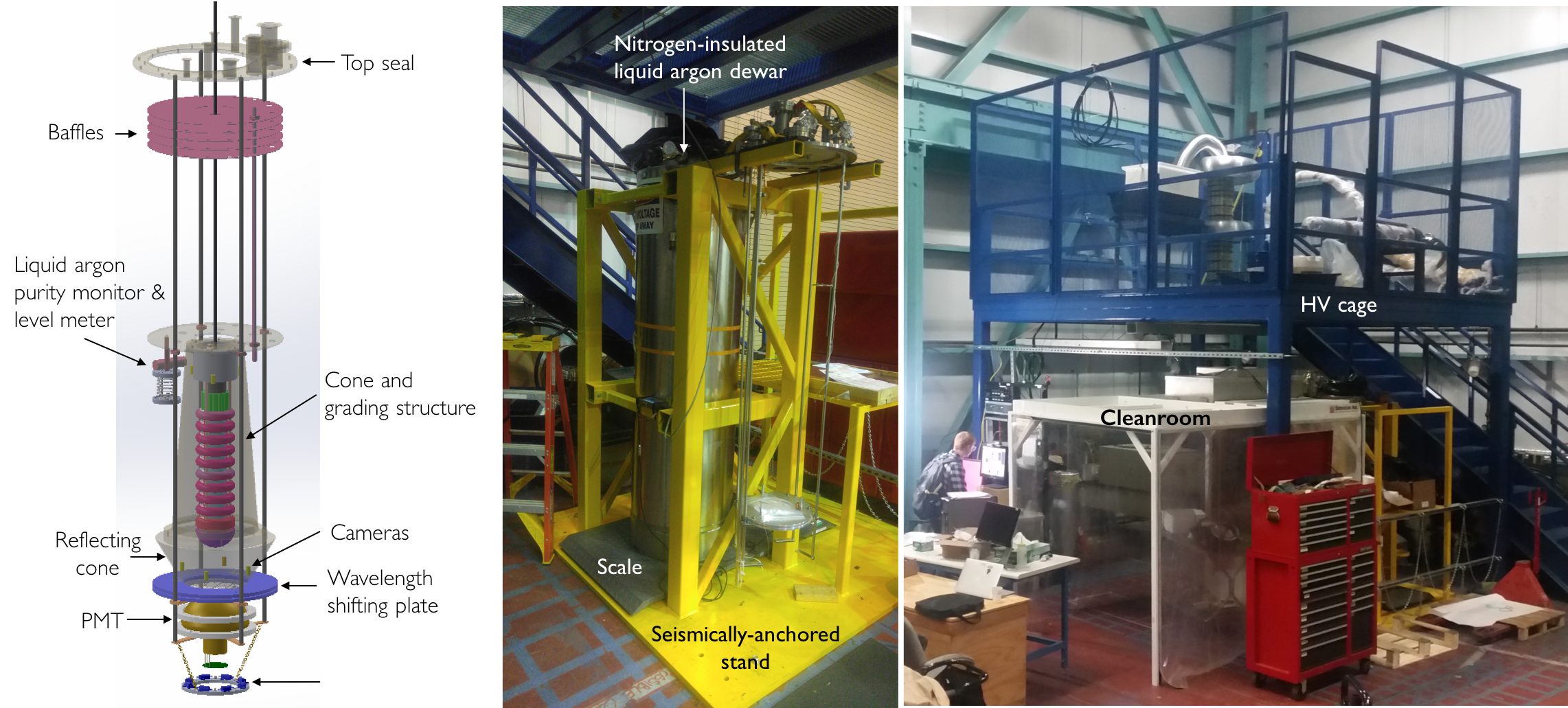
Figure 5.15: Setup used for testing of the cone and grading structure of the LZ feedthrough. Left: CAD rendering of the test structure. Baffles on top improve thermal insulation of the inside volume. The boil-off heater located near the bottom is used to accelerate LAr evaporation once the tests are completed. Center: The test structure is located inside a vacuum-insulated, nitrogen-jacketed dewar filled with LAr during tests. The dewar is placed inside the seismically-anchored yellow stand. The scale provides a measurement of the amount of LAr in the dewar. Right: The test stand is located under the HV cage in the platform (blue structure) built for these tests in building 77A at LBNL.

5.2 High voltage breakdown dependence on liquid noble purity

There is evidence that dielectric breakdown in LAr depends on the noble liquid purity [313, 314, 315]; a smaller amount of impurities can trigger breakdowns at lower fields compared to more polluted LAr as seen in Figure 5.16. Therefore, in order to validate results from the HV feedthrough tests described in Section 5.1.3.1, it is important to know the purity of the LAr present in the dewar. Since the setup itself cannot infer LAr purity directly, a standalone purity monitor was needed for the purity measurements. The following section details the design, construction, and performance of this purity monitor.

The purity monitor is an integral part of the system that allows a fast and reliable measurement of electronegative contaminants both in LAr or LXe. Three purity monitors have been built at Yale University and LBNL. I developed the first purity monitor for the LZ cold grading structure test. A close copy of the first purity monitor was built for the XeBrA experiment, described in Chapter 6, by Glenn Richardson, undergraduate advisee from UC Berkeley. Some of the improvements and technical details of the XeBrA purity monitor are outlined in Section 5.4. Furthermore, a third purity monitor that very closely follows the design of the XeBrA purity monitor is currently under construction for the Immersed BRIDF Experiment in Xenon (IBEX) optical experiment at LBNL. The subsequent sections describe the design, construction, and results from these purity monitors.

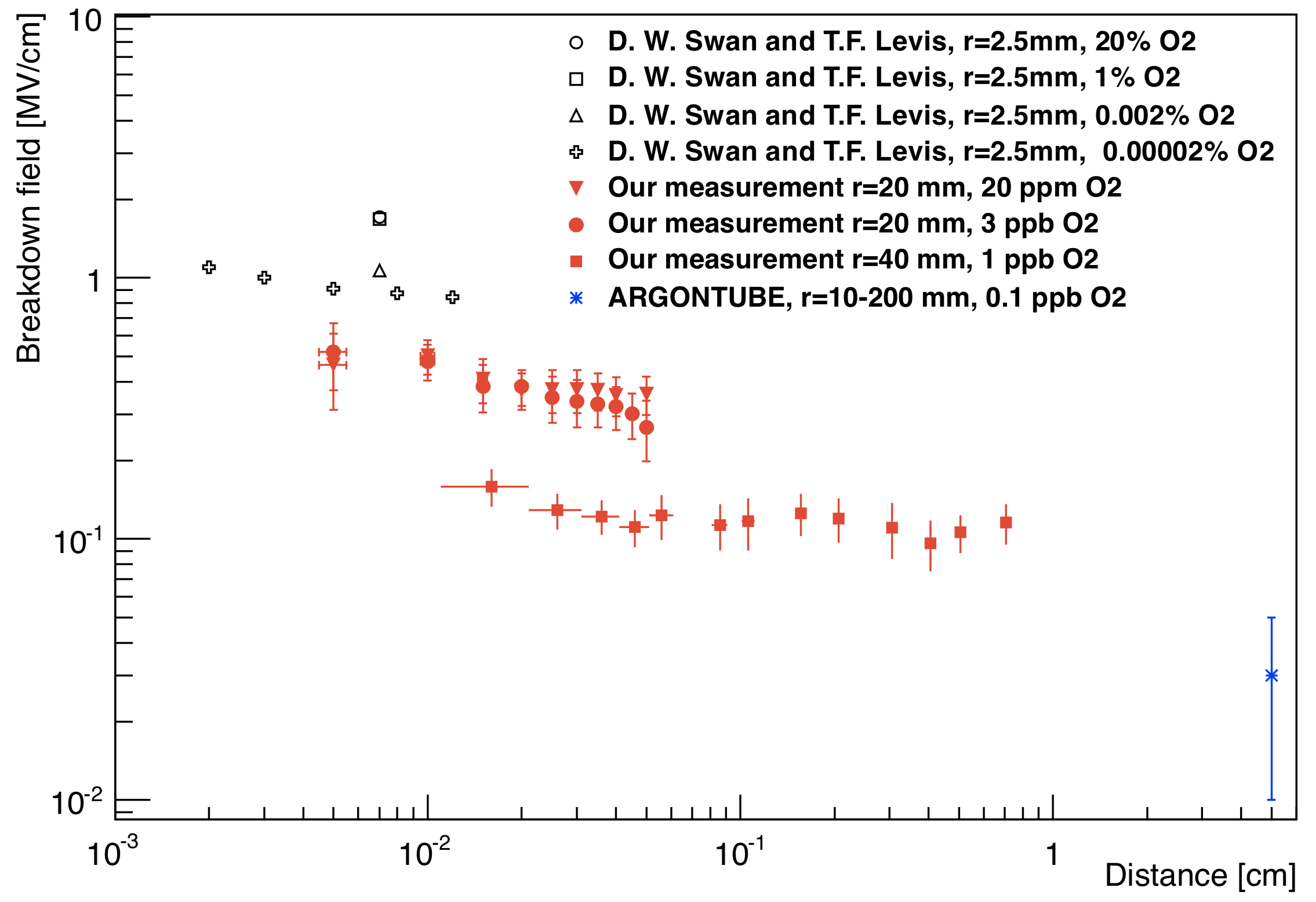
Figure 5.16: Compilation of experimental data showing measurements of HV breakdown at various LAr purities. The variable $r$ indicates the radius of the cathode used in the tests. Figure from [313].

5.3 Design and operating principles of liquid noble purity monitors

The purity monitor is a small double-gridded drift chamber fully submerged in liquid. Electrons are extracted from a photocathode via the photoelectric effect and drifted along electric field lines toward the anode. The electrons cross two mesh grids on the way. The first grid shields the rest of the detector from the electrons generated on the cathode. The effect of the second grid is to shield the anode from the drifting electrons so that a signal is induced on the anode only after the electrons have crossed the grid, hence creating a well-defined signal. The number of electrons decreases during this drift period as they attach to impurities. This enables the determination of electron lifetime $\tau$, which is a function of the ratio of electrons arriving at the anode to the number of electrons emitted at the photocathode. In practical use, the electron lifetime $\tau$ can also be converted to the total oxygen-equivalent concentration of impurities.

This section provides a detailed overview of the construction of two purity monitors along with their technical details and a theoretical derivation of their operating principles. The purity monitor described in this section was inspired by many purity monitors built by other collaborations for both LAr and LXe as described in [316, 317, 318, 319, 320, 321], among others. The purity monitor is a relatively inexpensive way to measure liquid noble purity if used with a xenon flash lamp.

5.3.1 Purity monitor system design

A schematic diagram of the purity monitor developed for the LZ HV tests at LBNL is shown in Figure 5.17. Electrons are extracted from a $1\,\mathrm{\mu m}$ thick gold layer deposited on a copper disk cathode using either a 266 nm laser or a xenon flash lamp coupled to a silica optical fiber. The electrons then drift toward the anode. The main drift region is 5-cm in length, enclosed by four brass field shaping rings. The anode is made of copper. Both the cathode and the anode are capacitively coupled to the same charge amplifier. The purity monitor is assembled on three Delrin rods, and the individual elements are held apart using Teflon spacers. A photograph of the assembled purity monitor can be seen in Figure 5.18.

As the electrons leave the cathode and move toward the cathode shield grid, an induced cathode current is detected by the charge amplifier. Once the electron cloud passes the anode shield grid, the charge amplifier detects another current pulse as the cloud approaches the anode. HV is supplied independently to the cathode and the anode through HV filter boxes (circuit details are outlined in Figure 5.19). The anode voltage is stepped down by a series of resistors to provide voltage to the anode shield grid and the field shaping rings. Initially, all three capacitors used in the purity monitor were made from metalized polypropylene but were later changed for X7R ceramic type capacitors [322] to reduce outgassing. The technical details of the purity monitor are summarized in Table 5.4, and a more detailed discussion of the individual components follows.

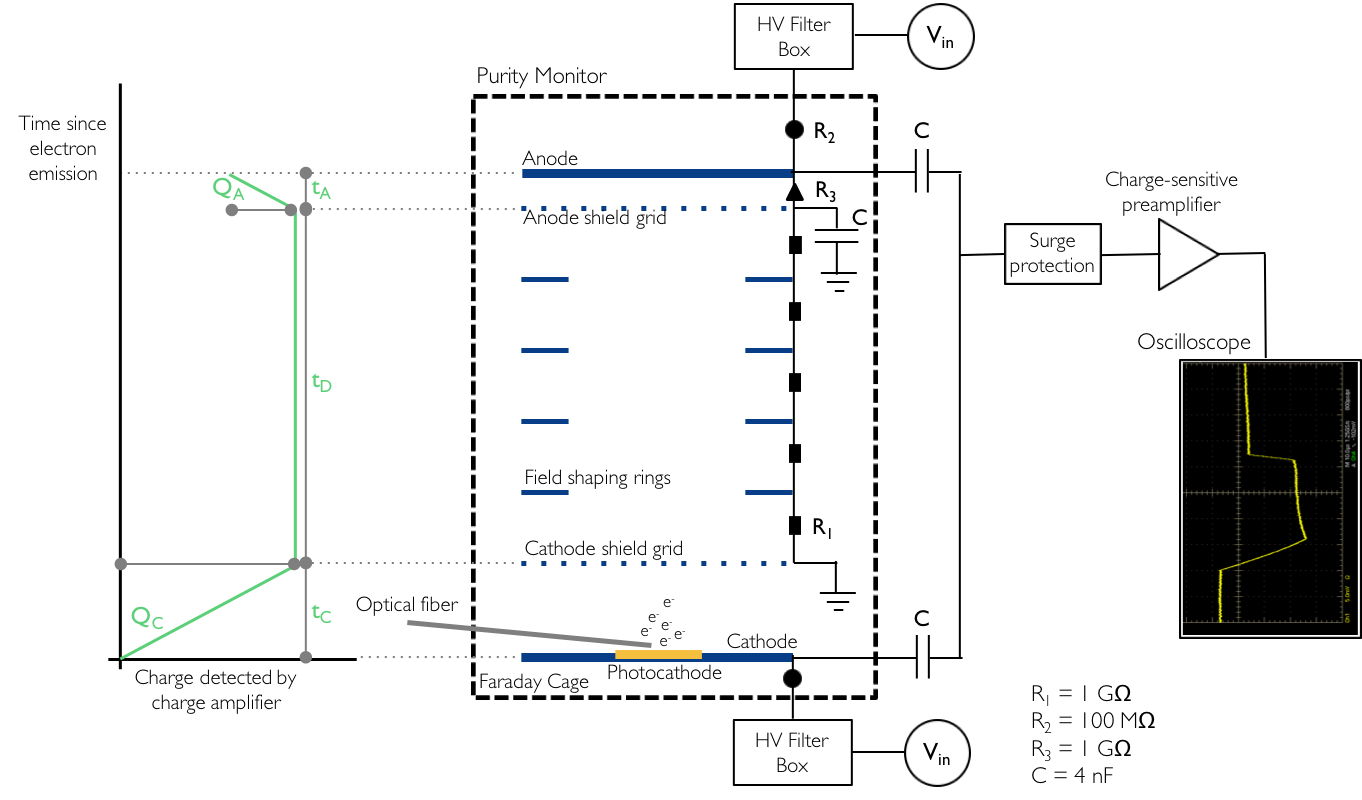
Figure 5.17: Schematics of the purity monitor and its readout system. The plot on the left illustrates the ideal signal detected by the purity monitor while a real image from an oscilloscope is shown on the right. The real signal includes the characteristic exponential RC decay of the charge amplifier used to read out the signal visible during the drift period of electrons, $t_{D}$.

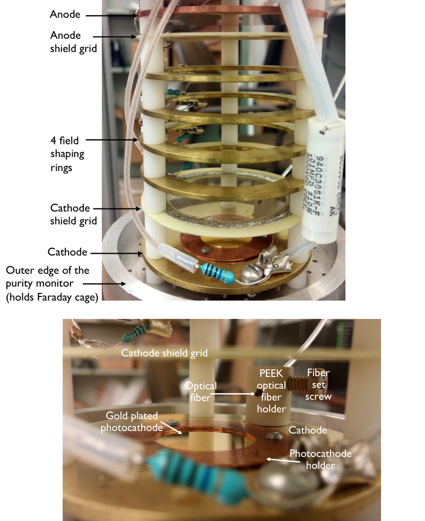
Figure 5.18: Top: Annotated image of the assembled purity monitor without its Faraday cage. Shown is the early version with a plastic capacitor (white cylinder). Bottom: Detail of the purity monitor cathode. The PEEK fiber holder is set such that the optical fiber points at the photocathode with a $10^{\circ}$ angle. The photocathode disk can be changed and is attached to the cathode using a copper clamp.

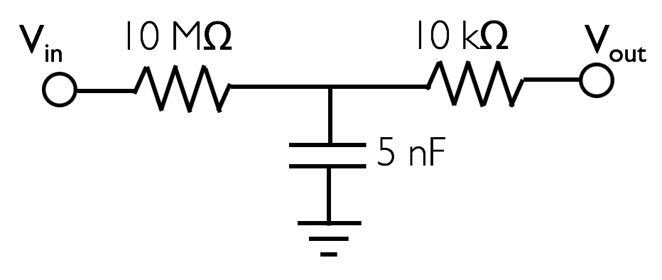
(a) HV filter box circuit.

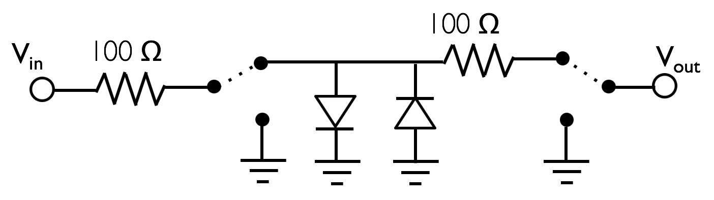
(b) Surge protection circuit.

Figure 5.19: Detailed circuit diagrams for electronic components introduced in Figure 5.17.

Purity monitor geometry
Cathode & anode diameter	57.0 mm
Photocathode diameter	20.0 mm
Cathode - cathode shield grid	15.0 mm
Cathode shield grid - anode shield grid	51.7 mm
Anode shied grid - anode	4.5 mm
Cathode - anode distance	71.2 mm
Number of field shaping rings	4
Shield grids
Grid wire diameter	50 $\mu$m
Grid wire spacing	500 $\mu$m
Photocathode	Au deposited on Cu
Deposit thickness	1.3 $\mu$m
WAu	5.1 eV = 243 nm
Laser	CryLaS FGSS 266-Q4_1k
Wavelength	266 nm
Pulse duration	$\leq 1$ ns
Pulse energy	$\geq 12$ $\mu$J at 1 kHz
Flash lamp	Hamamatsu L9455-11
Spectral distribution	185 - 2000 nm
Energy per flash	17.6 mJ
Optical fiber	JT Ingram Technologies Inc.
Material	Silica
Fiber core diameter	1 mm
Static bend radius	27.5 cm
Total length used	1 m outside + 60 cm inside
Angle between fiber and photocathode	10∘
Charge amplifier	Cremat CR-110
Decay time constant	140 $\mu$s
Gain	1.4 V/pC
Oscilloscope	Tektronix TDS5034B
Design Electric Fields
Cathode - Cathode shield grid	250 V/cm
Cathode shield grid - Anode shield grid	500 V/cm
Anode shield grid - Anode	1,000 V/cm

Table 5.4: Parameters of the purity monitor used for LZ HV tests in LAr.

5.3.1.1 Electron extraction

The photocathode consists of a gold-plated copper disk located in the center of a brass cathode as seen in Figure 5.18. Either a 266 nm (4.7 eV) laser or a xenon flash lamp can be coupled to a silica fiber to extract electrons from the photocathode. The spectral distribution of the xenon flash lamp ranges from $\lambda\sim 185-2000\,\mathrm{nm}$ ($6.7-0.6$ eV) with the emission peak located around $\lambda\sim 240\,\mathrm{nm}$. Figure 5.20 shows the timing profile of the xenon flash lamp pulse and the attenuation of the silica fiber used. Properties of the laser, the xenon flash lamp, and the optical fiber are summarized in Table 5.4. The laser provides a monoenergetic peak and has a widely tunable pulse intensity, while the flash lamp produces a much broader spectrum but at a fraction of the cost of the laser. The broader spectrum also includes shorter wavelengths, which is desired for this application, so the flash lamp is the light source used for operations of all the purity monitors.

The work function of pure gold is $W_{Au}=5.3-5.5\,\mathrm{eV}$ [323], but values down to 4.7 eV have been reported when impurities are present in the substrate [324]. The photoelectric effect used to extract electrons from the cathode can be seen by varying the laser power as shown in Figure 5.21. Also shown in the figure is the number of extracted electrons from the photocathode as a function of the electric field in the cathode region assuming a charge amplifier gain of 1.4 V/pC [325].

A solid silver disc was tried as a photocathode since the work function $W_{Au}\sim 4.5\,\mathrm{eV}$ is lower than that of gold. However, no signal was seen, likely due to a rapid formation of an oxidation layer prior to submersion in LAr.

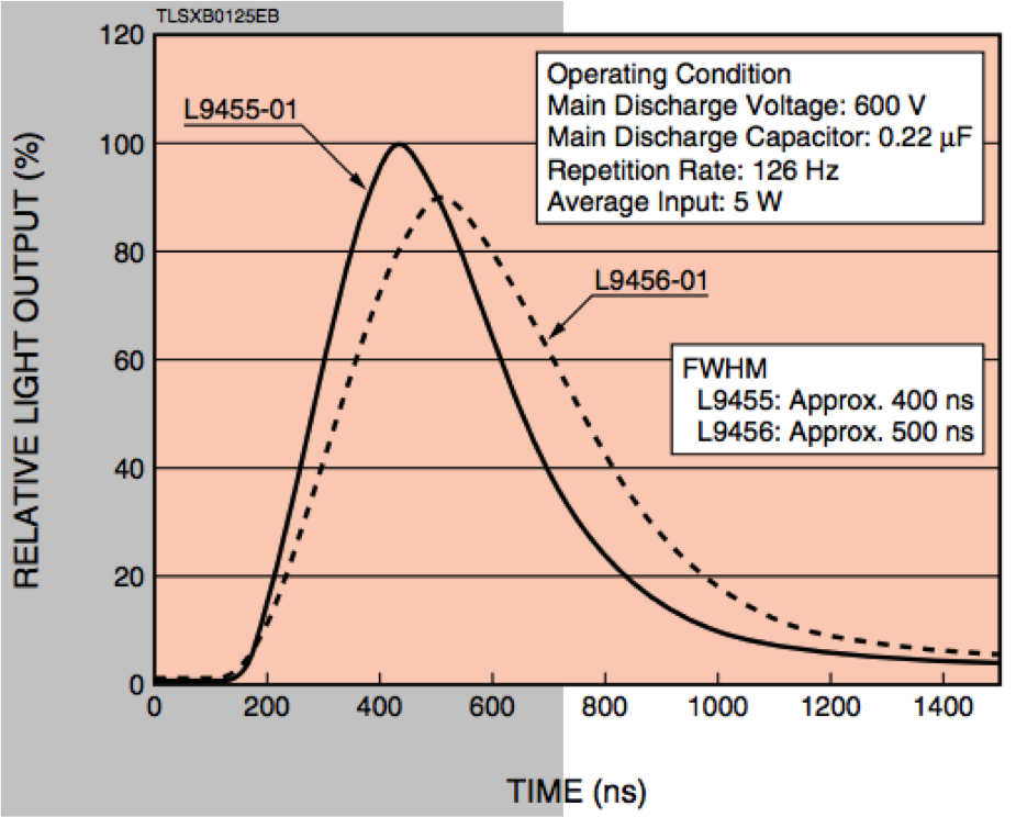
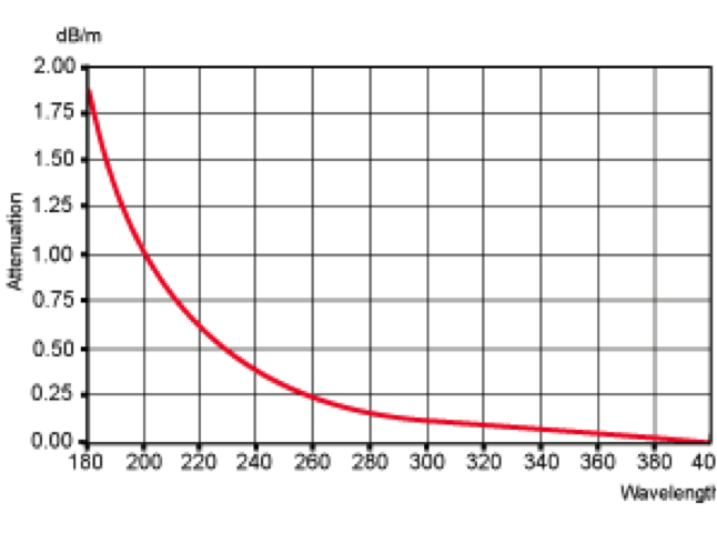
Figure 5.20: Left: Flash pulse waveform of the xenon flash lamp from Hamamatsu L9455-11 [326]. Right: Silica fiber transmission for UV light [327].

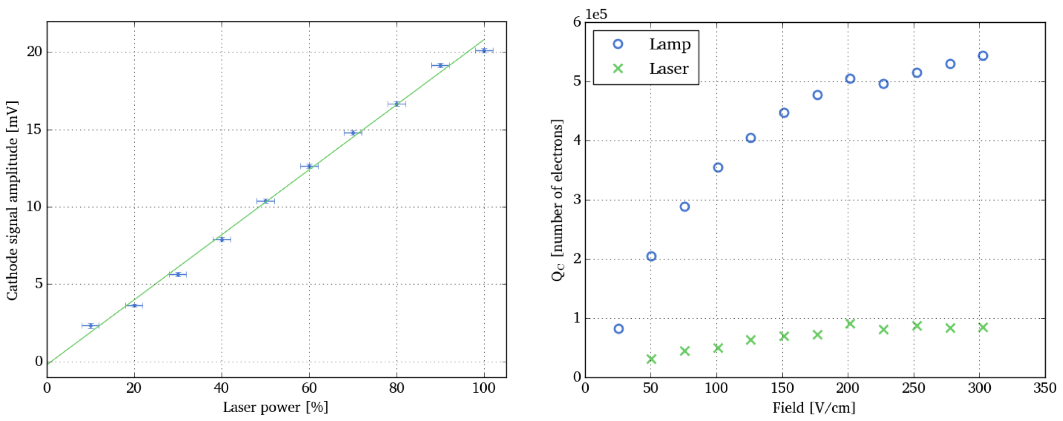
Figure 5.21: Left: Signal amplitude detected on the cathode as a function of laser power. Right: Extracted charge $Q_{C}$ as a function of the electric field between the cathode and the cathode shield grid for laser (green crosses) and xenon flash lamp (blue circles).

A drawback of the solid gilded metal cathode is that the optical fiber needs to enter from the side, adding design complexity since the silica fiber is not very flexible. An alternative is to use a semi-transparent photocathode where gold is evaporated onto a sapphire disk, such as was done in [320]. This design was not tried but would allow the optical fiber to enter the purity monitor on axis.

5.3.1.2 Grids

The shield grids have a wire diameter $d=50\,\mathrm{\mu m}$ and spacing between wires $a=\mbox{$500\,\mathrm{\mu m}$}$ resulting in an optical transparency of 83%. To assure that no field lines end on the shield grids, the field difference between each neighboring region must be adequately large. For grids with parallel wires, a 100% transparency to drifting electrons is achieved if the ratio of neighboring electric fields is

$$\frac{E_{A}}{E_{B}}\geq\frac{1+\rho}{1-\rho}\left[\frac{1+\frac{a}{4\pi D_{A}}\left(\rho^{2}-4\ln\rho\right)}{1+\frac{a}{4\pi D_{B}}\left(\rho^{2}-4\ln\rho\right)}\right]$$ (5.1)

where $E_{A}$ is the field after the grid, $E_{B}$ is the field before the grid, $a$ is the grid pitch, $D_{A}$ and $D_{B}$ are the lengths of regions $A$ and $B$, and

$$\rho=2\pi\frac{r}{a}$$ (5.2)

where $r$ is the grid wire radius [328, 329].

However, the grids in the purity monitor are crossed-wire meshes, so a correction needs to be introduced. This correction is presented in [329] as an empirical rule, where $\rho$ needs to be multiplied by two so that $\rho_{mesh}=2\rho$. Unfortunately, this correction was only discovered after the testing of the purity monitor was complete. As a result, all plots presented in this section have a loss of charge to the shield grids unaccounted for, which slightly reduces the estimated electron lifetime.

This error was corrected before the deployment of the purity monitor in the 77A test stand by replacing the $R_{3}=1\,\mathrm{G\Omega}$ resistor from Figure 5.17 between the anode and the anode shield grid by a $2\,\mathrm{G\Omega}$ resistor and an appropriate choice of bias voltages $V_{in}$. The new resistor results in a field ratio $\mathrm{E_{A}/E_{B}=4.4}$.

5.3.1.3 Anode feedthrough connection

In order to achieve a wide range of purity measurements, the purity monitor was designed to operate with up to 3 kV on the anode. It has been empirically observed that argon and xenon gas exhibit low dielectric strength. Therefore, particular care needs to be taken when using HV feedthroughs in argon gas. A smooth-edged cylinder pictured on Figure 5.22 was designed with $r=R/e$ where $r$ is the radius of the field-optimizing cylinder, and $R$ is the radius of the KF nipple serving as the HV feedthrough connection, and $e\simeq 2.72$ is Euler’s number. When assembled, the field-optimizing cylinder is located in the center of the KF nipple, and the HV cable then connects to the purity monitor attached to the flange as shown on the picture. This field-optimizing cylinder improved the voltage profile of the feedthrough, and the system was able to deliver up to 3,700 V in gaseous argon.

5.3.1.4 Level sensor

The purity monitor needs to be fully submerged in LAr during operation. To monitor the level of LAr in the experimental cryostat, a simple level sensor was designed consisting of two rolled up layers of 2 each of a $50\,\mathrm{\mu m}$ copper sheet and a polypropylene plastic mesh with 32% transparency. This creates a rolled up parallel plate capacitor with $C=2.1\,\mathrm{nF}$ while in air, vacuum or gaseous argon and $C=2.8\,\mathrm{nF}$ while fully submerged in LAr. The level sensor was only used to determine whether the purity monitor was fully submerged in liquid argon. Figure 5.22 shows the level sensor inserted in a Delrin tube to prevent unrolling next to the purity monitor.

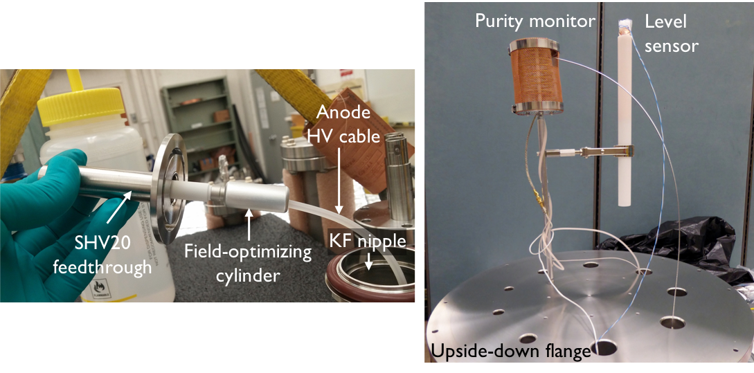
Figure 5.22: Left: Field-optimizing cylinder designed to optimize electric fields inside a KF40 nipple. Right: Purity monitor setup alongside the liquid level sensor attached to a flange. Also visible is the cutout in the Faraday cage for the optical fiber.

5.3.1.5 Electronics

To ensure that electrons generated on the cathode travel through LAr to the anode while the signal can also be sensed by the charge sensitive preamplifier, the design requires that $Z_{C}\ll Z_{LAr}\ll R_{HV}$. Here $R_{HV}=100\,\mathrm{M\Omega}$ ($R_{2}$ in Figure 5.17). $Z_{LAr}$ is the impedance of the LAr layer between the cathode and the cathode shield grid:

$$\left|Z_{LAr}\right|=\left|\frac{1}{j\omega C_{LAr}}\right|=3.5\,\mathrm{M\Omega}.$$ (5.3)

The capacitance of LAr, $C_{LAr}$, is given by

$$C_{LAr}=\varepsilon_{0}\varepsilon_{r\,LAr}\frac{A}{d}=2.3\,\mathrm{pF}$$ (5.4)

where $\varepsilon_{0}=8.85\times 10^{-12}\,\mathrm{F/m}$ is the permittivity of vacuum, the relative permittivity of LAr is $\varepsilon_{r\,LAr}=1.5$, and $\omega=2\pi f$ with $f\sim 20\,\mathrm{kHz}$ corresponds to an average drift time of electrons between the cathode and the cathode shield grid with $t_{C}=50\,\mathrm{\mu s}$. $Z_{C}=2\,\mathrm{k\Omega}$ is the impedance of the coupling capacitor (C in Figure 5.17) assuming $f=20\,\mathrm{kHz}$. A simplified electronic circuit of the cathode region is shown in Figure 5.23.

Figure 5.23: Schematics of the electronics surrounding the purity monitor cathode. The current source are electrons created via the photoelectric effect and the charge amplifier can be approximated as an ammeter.

There are three capacitors installed in the purity monitor. Two capacitors prevent current from the cathode and anode power supplies from entering the charge amplifier. The third capacitor holds the anode shield grid at a stable voltage. The grids can only work as a shield if they can be held at a stable voltage on fast timescales of $\mathcal{O}\left(\mu s\right)$ corresponding to the electron drift time. Without the third capacitor in place, the voltage on the shield grid decreases as electrons approach and the grid loses its function shielding anode from those drifting electrons.

Signal read out:

Both the cathode and the anode are coupled through a capacitor and a surge protection box to a Cremat CR-110 charge sensitive pre-amplifier. The light source is configured to emit pulses at $\sim 10\,\mathrm{Hz}$, and the resulting signal is connected directly into a Tektronix oscilloscope. The oscilloscope averages all the signals used in the analysis and the subsequent data analysis is performed using Python package v2.7.

5.3.1.6 Electric field simulation

An axially symmetric electric field simulation of the purity monitor was created in COMSOL Multiphysics, similar to those built in Chapter 3, to confirm that electric fields within the region of interest were uniform. The results of the simulation are shown in Figure 5.24.

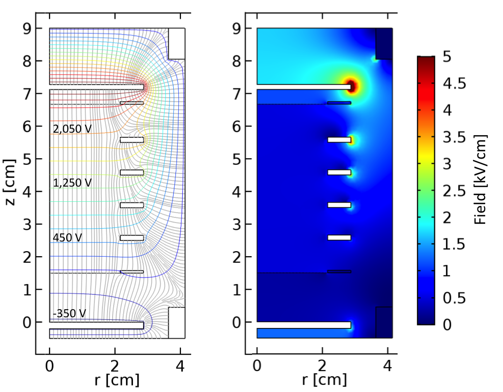
Figure 5.24: Simulations from an axially symmetric COMSOL model of the electric fields inside the purity monitor Left: Electric field lines and equipotential contours for $E_{D}=500\,\mathrm{V/cm}$. Right: Electric field of the purity monitor with -375 V on the cathode, 2,500 V on the anode shield grid and 3,000 V on the anode. The highest field value is 10.8 kV/cm at the edge of the anode.

5.3.2 Purity monitor testing

The space needed at LBNL for purity monitor tests in LAr was set up so that commercially available LAr flowed through a purifier into a test cryostat as shown in Figure 5.26. To reduce the amount of LAr needed to fill the cryostat, the tests were conducted inside a 22-liter stainless steel pot hanging from the flange of the cryostat as shown in Figure 5.26. The cryostat was evacuated before every fill to reduce impurities in LAr.

To simplify operations and to reduce costs, the testing setup did not use a closed circulation system. Instead, commercially available 99.999% pure liquid argon was used for the test, corresponding to $\mathcal{O}\left(\mathrm{ppm}\right)$ of oxygen equivalent impurity concentration. Since the purity monitor was designed to detect impurities $\mathcal{O}\left(\mathrm{ppb}\right)$, a purifier described in Section 5.3.3 was used to reach the desired LAr purity. The purification is done in-line with LAr flowing from a commercial LAr dewar through the purifier directly into the well-insulated cryostat where it slowly evaporates once the testing is over.

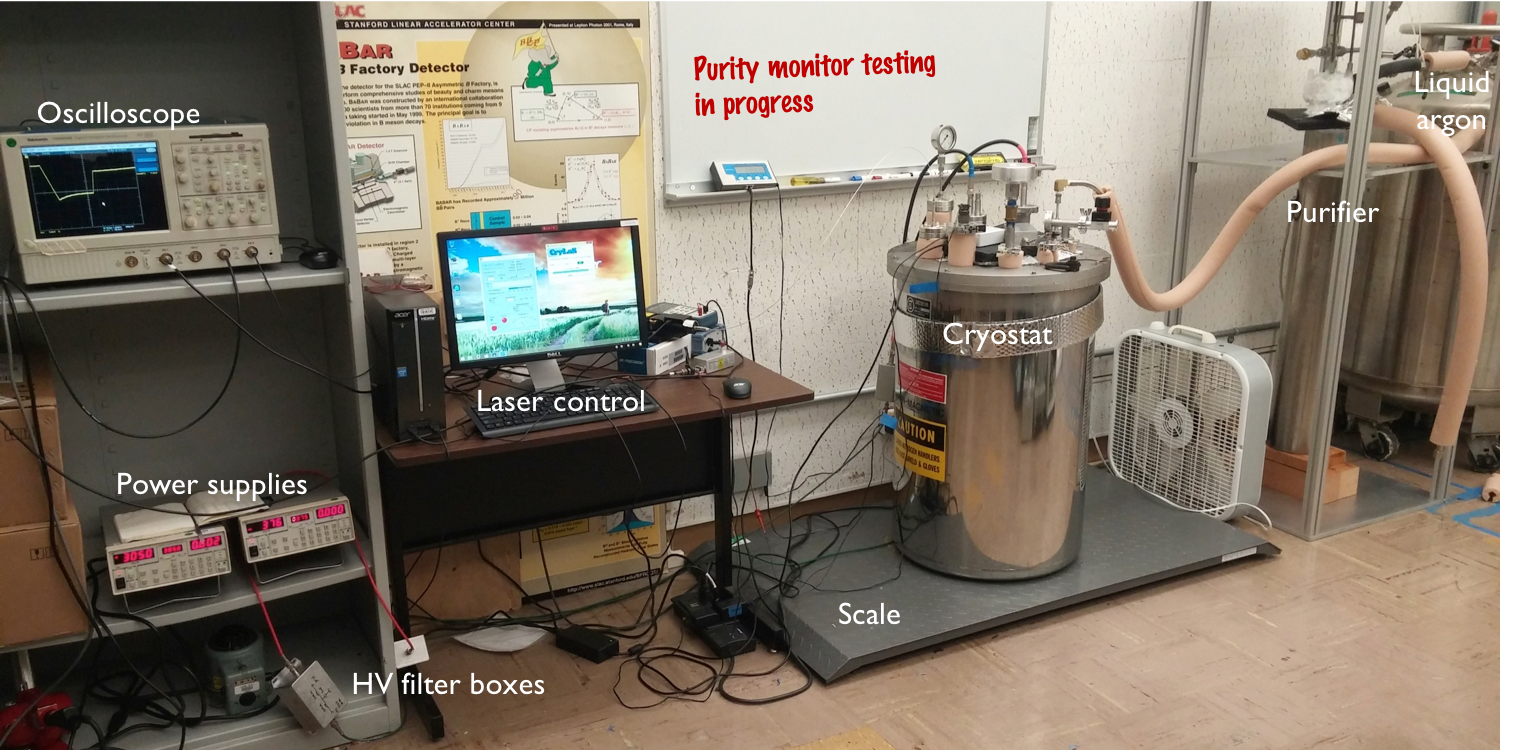
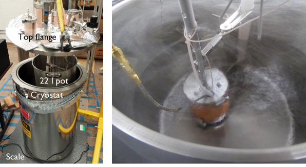
Figure 5.25: Lab layout for purity monitor testing. Liquid argon from a commercial dewar flows through the purifier into the cryostat shown in the center. Also shown on the left are the power supplies and the data readout.

Figure 5.26: Left: Purity monitor inside a 22 L stainless steel pot inside a cryostat. The scale measured the amount of liquid argon in the cryostat. Right: Purity monitor submerged in LAr.

5.3.3 Liquid argon purifier

The inline purifier is designed to remove O₂ and H₂O from either gaseous or liquid argon. The filter, built at Yale University, is filled with molecular sieve material and activated copper following the design of [330]. Once the filter particles are saturated with impurities, the filter can easily be regenerated in situ and used again at full capacity. Details of this purifier are described below.

Molecular sieve:

The molecular sieve is a zeolite, a highly porous crystalline aluminosilicate with three-dimensional, identical pores of precisely defined diameter. The sieve has a high adsorption capacity for liquids and vapor. Due to the molecule geometry the sieve can capture in its center molecules small enough to permit passage through the pore, i.e. molecules with diameter smaller than 4 $\mathring{\mathrm{A}}$ such as O₂ (d = 3.5 $\mathring{\mathrm{A}}$), H₂O (d = 2.7 $\mathring{\mathrm{A}}$), N₂ (d = 3.6 $\mathrm{\mathring{\mathrm{A}}}$) or CO₂ (d = 3.3 $\mathrm{\mathring{\mathrm{A}}}$). Additionally, hydrophilic substances experience stronger adsorption. The number of impurities the molecular sieve is able to hold decreases with increasing temperature as illustrated in Figure 5.27.

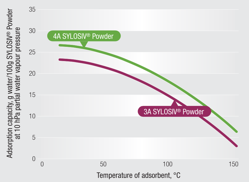
Figure 5.27: The adsorption capacity of molecular sieve at different temperatures. 4A SYLOSIV^® Powder was used in the purifier. Figure from [331].

Activated copper:

Activated copper removes oxygen by exothermic copper oxidation

$$4\,\mathrm{Cu+O_{2}} \rightarrow 2\,\mathrm{Cu_{2}O}+2*156\,\mathrm{kJ/mol}$$ (5.5)

$$2\,\mathrm{Cu}+\mathrm{O_{2}} \rightarrow 2\,\mathrm{CuO}+2*170\,\mathrm{kJ/mol}.$$ (5.6)

The amount of bound oxygen is limited, but this process can be reversed by flushing the purifier with hydrogen gas while providing heat according to [332]:

$$\mathrm{CuO}+\mathrm{H_{2}}\overset{\mathrm{heat}}{\rightarrow}\mathrm{Cu}+\mathrm{H_{2}O}+\mathrm{heat}$$ (5.7)

Activated copper was purchased from Engelhard Corporation as a composite of alumina and copper oxide with 14 x 28 mesh beads. The alumina forms a very porous structure providing an inert support to a thin layer of copper deposited on top.

5.3.3.1 Purifier conditioning

This type of purifier is fully regenerable. The filter can be regenerated through evacuation while heated at $250^{\circ}$C for several hours and then flowing hydrogen through the purifier. A detailed description of the regeneration process that was followed is available in [320, 330]. It was found that the most significant improvement in the regeneration process was achieved by heating the purifier while evacuated, prior to flowing the Ar-H mixture.

It is essential to monitor the temperature of the purifier throughout its entire height since a large temperature gradient can develop if the heating tape is not installed uniformly. This lesson was learned when the bottom of the purifier was heated up beyond the recommended $250^{\circ}$C, as was determined by the coloration of the stainless steel container. Overheating can cause the activated copper to anneal, thus greatly reducing the exposed surface area that binds oxygen.

5.3.4 Theoretical motivation for purity monitor operations

The core of the purity monitor operations relies on accurate measurements of electrons generated at the cathode and the number of electrons not captured by impurities on the way to the anode. This section first characterizes the attachment of electrons to impurities and then derives the formula for calculation of electron lifetime from the current detected on the purity monitor’s cathode and anode.

5.3.4.1 Electron attachment to impurities

Following the derivation from [333] the electron attachment to an impurity $S$ can be described by

$$e^{-}+\mathrm{S}\underset{k_{S}}{\rightarrow}\mathrm{S}^{-}$$ (5.8)

with the rate constant $k_{S}$

$$k_{S}=\int v\sigma(v)f(v)dv$$ (5.9)

where $v$ is the instantaneous electron velocity (not the average drift velocity), $f(v)$ is the velocity distribution of the electrons and $\sigma(v)$ is the electron-impurity interaction cross-section. This causes $k_{S}$ to vary as a function of an external electric field as illustrated in Figure 5.28. Assuming that the number of electrons $N$ produced by the photoelectric effect is much smaller than the impurity concentration $N_{S}$, the number of electrons lost over time is

$$\frac{dN}{dt}=-k_{S}N_{S}N.$$ (5.10)

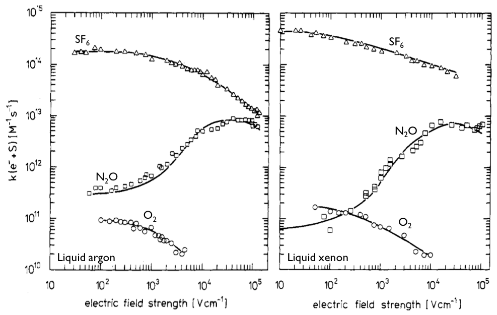
Figure 5.28: Rate constant for the attachment of electrons to several solutes. It is expected that the main impurities present in LAr and LXe are O₂, N₂, and $\mathrm{H_{2}O}$ (the latter two are not included in the plot). Left: In LAr at 87 K. Right: In LXe at 165 K. Figures from [334].

For regular purity monitor operations, the number of impurities $N_{S}$ is assumed to be constant during data taking. Therefore integrating Equation 5.10 leads to

$$N=N_{0}e^{-t/\tau}$$ (5.11)

where $\tau$ is the electron lifetime and is related to the impurity concentration and rate constant by

$$\tau=\frac{1}{k_{S}N_{S}}.$$ (5.12)

As a result of this process, electrons trapped by impurities create negative ions that have a much smaller mobility. Depending on the purity of the liquid, a signal from the electrons can then be measured on the cathode and the anode of the purity monitor. The conspicuous decrease in the amplitude of the electron signal on the anode due to the conversion of electrons into ions is used to measure the presence of impurities in the intervening fluid.

5.3.4.2 Electron lifetime to oxygen-equivalent impurity concentration conversion

In some publications, the purity of the liquid is stated as a function of electron lifetime, while in others a unit of oxygen-equivalent impurities is used. Equation 5.12 can be used to convert the electron lifetime $\tau$ to an equivalent concentration of impurities in units of mol/l. The following calculation follows the community standard and assumes that oxygen accounts for 100% of impurities present, even though we expect nitrogen and other impurities to be present in the liquid as well. The concentration of impurities $N_{S}$ is related to the concentration $\rho$ in units of ppb by

$$\rho = \frac{N_{S}}{N_{Ar}}$$ (5.13)

$$\rho = \frac{1}{k_{S}N_{Ar}}\frac{1}{\tau}$$ (5.14)

as defined in [333]. $N_{Ar}$ is the number of moles in $V=1\,\mathrm{liter}$ of liquid argon

$$N_{Ar} =\frac{\rho_{LAr}V}{M_{Ar}}=35\,\mathrm{mol}$$ (5.15)

since the molar mass of argon is $M_{Ar}=39.95\,\mathrm{g/mol}$ and LAr density $\rho_{LAr}=1.4\,\mathrm{g/cm^{3}}$ at its boiling point of 87.3 K at 1 atm. The rate of attachment of impurities can be obtained from Figure 5.28 with $k_{S}\sim\text{$7\times 10^{10}\,\mathrm{l/\left(mol\cdot s\right)}$}$ for fields between $250-1000\,\mathrm{V/cm}$. Then from Equation 5.14

$$\rho_{LAr} \sim\frac{408}{\tau}\,\mathrm{\frac{ppb}{\mu s}}$$ (5.16)

where ppb is defined as one oxygen molecule in every $10^{9}$ argon atoms.

Similarly, for LXe the rate of attachment of impurities $k_{S}\sim\text{$1\times 10^{11}\,\mathrm{l/\left(mol\cdot s\right)}$}$ for fields between $250-1000\,\mathrm{V/cm}$. Therefore, the number of moles in 1 l of LXe

$$N_{Xe} =\frac{\rho_{LXe}V}{M_{Xe}}=22\,\mathrm{mol}$$

at the LXe boiling point of 165 K at 1 atm. Therefore,

$$\rho_{LXe}\sim\frac{455}{\tau}\,\mathrm{\frac{ppb}{\mu s}}.$$ (5.17)

5.3.4.3 Electron lifetime derivation

To find the formula for electron lifetime measured by the purity monitor, the charge on the cathode and anode can be derived from the current detected on those two electrodes as derived in this section. The current as a function of time $I(t)$ measured at the cathode (anode) is determined by the speed with which the electrons pass either the cathode or the anode shield grids where $v=\frac{d}{t_{j}}$ and $j\epsilon\left\{C,\,A\right\}$ stands for cathode (anode). The current detected at time $t$ is given by

$$I(t_{j})=N(t)e\frac{v}{d_{j}}=N(t)\frac{e}{t_{j}}$$ (5.18)

where $N(t)$ is the number of electrons contributing to the pulse as a function of time. There are 3 distinct time periods within the purity monitor: $t_{C}$ is the time it takes the electrons to travel from the cathode to the cathode shield grid, $t_{D}$ is the main drift travel time between the cathode shield grid and the anode shield grid and $t_{A}$ is the period between the anode shield grid and the anode.

The charge sensed at the cathode $Q_{C}$ is given by integrating the current between $t=0$ and $t=t_{C}$:

$$Q_{C}=\intop_{0}^{t_{C}}I(t)dt=N_{0}e\frac{v}{d}\intop_{0}^{t_{C}}e^{-t/\tau}dt$$ (5.19)

and the charge magnitude emitted from the photocathode is

$$Q_{0}=N_{0}e.$$ (5.20)

Since the electron drift velocity is constant between the cathode and the cathode shield grid, $\frac{v}{d}=\frac{1}{t_{C}}$ so Equation 5.19 becomes

$$Q_{C}=Q_{0}\frac{1}{t_{C}}\tau\left(1-e^{-t_{C}/\tau}\right).$$ (5.21)

The number of surviving electrons $N_{D}$ crossing the anode shield grid is

$$N_{D}=N_{0}e^{-t_{C}/\tau}e^{-t_{D}/\tau}$$ (5.22)

hence the charge $Q_{A}$ detected at the anode is given by

$$Q_{A}=\intop_{0}^{t_{A}}i(t)dt=N_{D}e\frac{v}{d}\intop_{0}^{t_{A}}e^{-t/\tau}dt.$$ (5.23)

Evaluating the integral gives

$$Q_{A}=Q_{0}\frac{1}{t_{A}}\tau\left(1-e^{-t_{A}/\tau}\right)e^{-t_{C}/\tau}e^{-t_{D}/\tau}.$$ (5.24)

The electron lifetime can now be found by calculating the ratio $R$ of the charge detected at the cathode and the anode:

$$R = \frac{Q_{A}}{Q_{C}}$$ (5.25)

$$R = \frac{t_{C}}{t_{A}}\frac{\left(1-e^{-t_{A}/\tau}\right)}{\left(e^{t_{C}/\tau}-1\right)}e^{-t_{D}/\tau}$$ (5.26)

$$R = \frac{t_{C}}{t_{A}}\frac{\sinh\left(\frac{t_{A}}{2\tau}\right)}{\sinh\left(\frac{t_{C}}{2\tau}\right)}e^{-\left(t_{D}+\frac{t_{A}+t_{C}}{2}\right)\frac{1}{\tau}}.$$ (5.27)

Generally, it is safe to assume that $t_{A},t_{C}\ll\tau$ due to the short distances between the cathode and cathode shield grid and the anode and anode shield grid. In this limit the first part of Equation 5.27 $\frac{t_{C}}{t_{A}}\frac{\sinh\left(\frac{t_{A}}{2\tau}\right)}{\sinh\left(\frac{t_{C}}{2\tau}\right)}\rightarrow 1$. Therefore, $R$ can be simplified to

$$R\simeq e^{-\left(t_{D}+\frac{t_{A}+t_{C}}{2}\right)\frac{1}{\tau}}$$ (5.28)

hence

$$\tau=-\frac{t_{W}}{\ln R}$$ (5.29)

where $t_{W}=t_{D}+\frac{t_{A}+t_{C}}{2}$. This result is in agreement with formulas presented in [316, 317].

5.3.5 Data analysis

An example of a signal trace from the LZ purity monitor fully submerged in LAr is shown in 5.29. The figure shows an annotated screenshot of the trace and its consequent analysis performed in Python. Each part of the trace was fitted with a $1^{\mathrm{st}}$, $2^{\mathrm{nd}}$ or $3^{\mathrm{rd}}$ degree polynomial and intersections of those curves help locate the boundary points for calculation of $t_{C}$, $t_{D}$, $t_{A}$, $Q_{C}$, and $Q_{A}$ . This particular trace was taken with the drift field at 500 V/cm and laser power at 90% resulting in $t_{C}=13.4\,\mathrm{\mu s}$, $t_{D}=33.1\,\mathrm{\mu s}$, $t_{A}=2.2\,\mathrm{\mu s}$, $Q_{C}=18.5\,\mathrm{mV}$, $Q_{A}=11.4\,\mathrm{mV}$ and $R=\frac{Q_{A}}{Q_{C}}=0.62$. Substituting these values in Equation 5.29 gives electron lifetime $\tau=85\pm 3\,\mathrm{\mu s}$, which based on Equation 5.16 corresponds to a concentration of oxygen equivalent impurities in LAr of $\sim 4.8\,\mathrm{ppb}$.

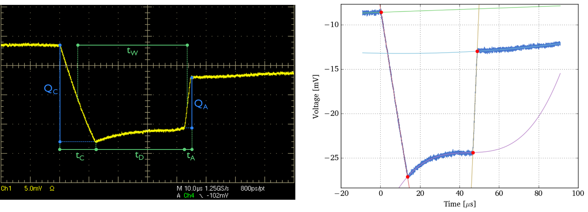
Figure 5.29: Left: Annotated example of a signal trace (yellow) from the oscilloscope averaged over 600 light pulses. $Q_{C}$ and $Q_{A}$ (blue) are the integrated charges at the cathode and the anode; $t_{C}$, $t_{D}$, and $t_{A}$ (green) are the transit times between cathode and cathode grid, cathode grid and anode grid, and anode grid and anode, respectively. $t_{W}$ is the FWHM of the overall signal. The smaller amplitude of $Q_{A}$ relative to $Q_{C}$ indicates the presence of impurities in LAr. The exponential decay apparent during $t_{D}$ arises from the RC decay constant of the charge amplifier. Right: Example fit used to find boundary points for data analysis. The found points are highlighted.

It should be noted that the calculations above assume a charge amplifier with an infinite decay time. In reality, the characteristic RC decay time constant is finite; the charge amplifier used in this work has a decay time constant of $140\,\mathrm{\mu s}$. This modifies the purity monitor signal as shown in Figure 5.29. This effect is visible in the segment of the signal where the drift time is not perfectly horizontal but instead slowly decays with this time constant. The cathode and anode signals are also affected by this finite decay time constant, but because of their short duration, this effect is not visible. For purity monitors with extremely long drift times (where $t_{C}$ and $t_{A}$ are on the order of the decay time constant), it might be necessary to calculate a correction. This can be done by convoluting the current on the cathode (anode) with the exponential decay of the charge amplifier to find the unaltered cathode (anode) signal.

5.3.5.1 Purity monitor resolution

The error on lifetime calculation is given by [316]:

$$\frac{\sigma_{\tau}}{\tau}=\sqrt{\left(\frac{1}{\ln R}\frac{\sigma_{R}}{R}\right)^{2}+\left(\frac{\sigma_{t_{W}}}{t_{W}}\right)^{2}}$$ (5.30)

assuming independence of $R$ and $t_{W}$. To find $\sigma_{R}$ and $\sigma_{t_{W}}$ dozens of measurements were recorded over a short period with the same settings. The deviation of $R$ and $t_{W}$ was determined to be $\sigma_{R}=0.012$ and $\sigma_{t_{W}}=0.357\,\mathrm{\mu s}$. To determine the error on lifetime accurately, multiple sets of measurements should be taken at each of the different voltage settings. For this analysis, the error was only determined at one voltage setting ($E_{D}=500\,\mathrm{V/cm}$ in the drift region).

A wide set of electric fields can be used to operate the purity monitor ranging from 25 V/cm in the cathode region up to 1200 V/cm in the anode region corresponding to total electron drift times of $40-200\,\mathrm{\mu s}$. For illustration Table 5.5 contains voltages, electric fields, and transit times for two different operating modes.

$V_{C}=-37.5\,\mathrm{V}$	$E_{C}=25\,\mathrm{V/cm}$	$t_{C}=100\,\mathrm{\mu s}$
$V_{AG}=250\,\mathrm{V}$	$E_{D}=50\,\mathrm{V/cm}$	$t_{D}=102\,\mathrm{\mu s}$
$V_{A}=300\,\mathrm{V}$	$E_{A}=100\,\mathrm{V/cm}$	$t_{A}=8\,\mathrm{\mu s}$

(a)

$V_{C}=-375\,\mathrm{V}$	$E_{C}=250\,\mathrm{V/cm}$	$t_{C}=13\,\mathrm{\mu s}$
$V_{AG}=2500\,\mathrm{V}$	$E_{D}=500\,\mathrm{V/cm}$	$t_{D}=33\,\mathrm{\mu s}$
$V_{A}=3000\,\mathrm{V}$	$E_{A}=1000\,\mathrm{V/cm}$	$t_{A}=2\,\mathrm{\mu s}$

(b)

Table 5.5: Voltages, electric field magnitudes, and transit times for two different operating modes of the purity monitor. Voltages on cathode, anode grid, and anode are shown along with electric field magnitudes and drift times in the three different purity monitor segments. The cathode shield grid is always grounded.

Ratio $R=\nicefrac{{Q_{A}}}{{Q_{C}}}$ is strongly related to LAr purity. When $R\rightarrow 0$ or $R\rightarrow 1$ the error on $\tau$ can be substantial. This can be seen in Figure 5.30 which illustrates the error on the lifetime as a function of $R$ when the purity monitor has 500 V/cm in the drift region and assuming the errors $\sigma_{R}$ and $\sigma_{t_{W}}$ quoted above. Figure 5.30 also shows the potential reach of the purity monitor for two different voltage settings. These plots show that the current purity monitor should be able to measure electron lifetime $\tau$ up to a millisecond with less than 10% error with $E_{D}=50\,\mathrm{V/cm}$ which corresponds to $\sim 0.4\,\mathrm{ppb}$ oxygen-equivalent impurities in LAr, well within the range needed for LZ & XeBrA.

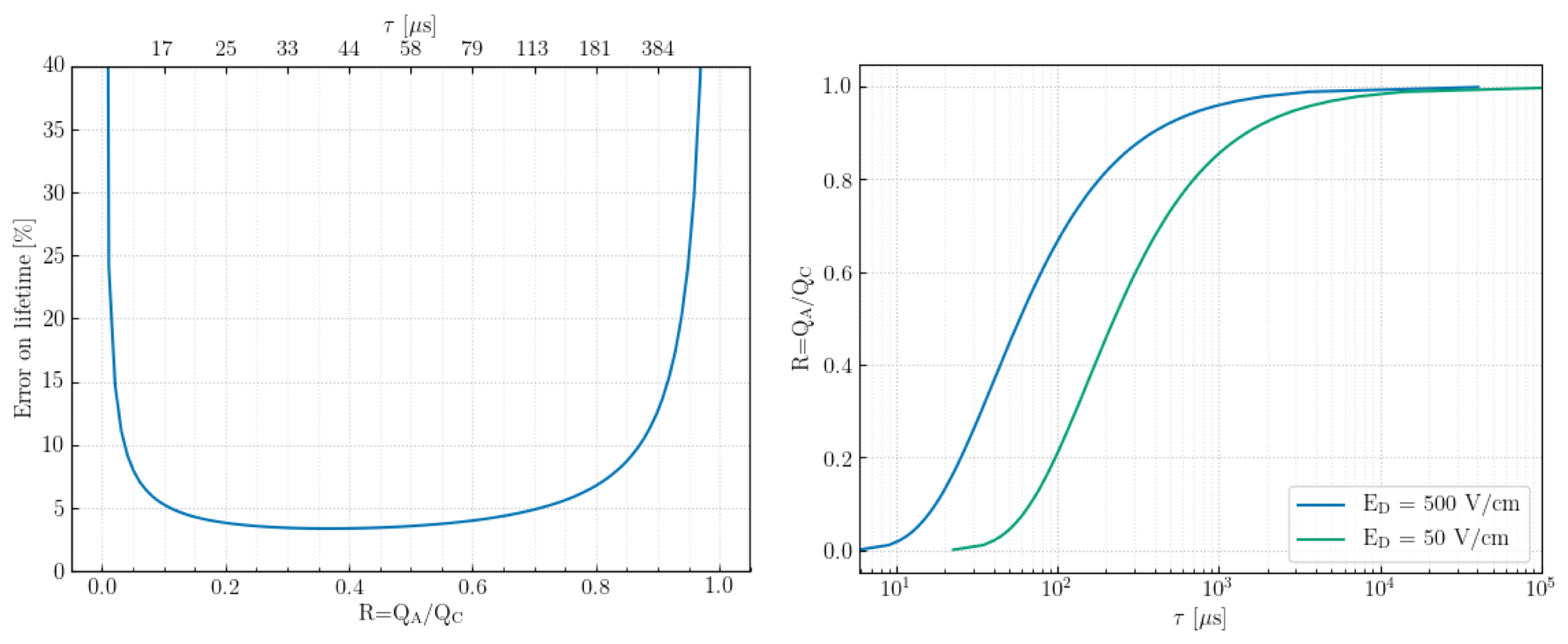
Figure 5.30: Left: The error on the lifetime versus the ratio $R=\nicefrac{{\mathrm{Q_{A}}}}{{\mathrm{Q_{C}}}}$ (bottom $x$ axis) for $E_{D}=500\,\mathrm{V/cm}$ and the estimated electron lifetime (top $x$ axis) for $t_{W}=40.5\,\mathrm{\mu s}$. Right: Ratio $R$ as a function of the electron lifetime for two different field settings assuming $t_{W}=40.5\,\mathrm{\mu s}$ at $E_{D}=500\,\mathrm{V/cm}$ and $t_{W}=156\,\mathrm{\mu s}$ at $E_{D}=50\,\mathrm{V/cm}$. The same error is assumed at $E_{D}=50\,\mathrm{V/cm}$ as was found for $E_{D}=500\,\mathrm{V/cm}$.

5.3.5.2 Electron lifetime dependence on electric field

Figure 5.31 shows several measurements of LAr purity performed over time at varying electric fields. Similar measurements were also performed by [316, 334]. There is a clear dependence of electron lifetime on the electric field, but this behavior is not yet thoroughly characterized in liquid argon and xenon.

It is unclear what are the dominant impurities present in LAr used for the tests described here. However, this measurement suggests that the purity monitor could be used to measure the effect of impurities on electron lifetime as a function of electric field if known amounts of impurities were injected into the system and the measurement was repeated for each impurity at a variety of fields.

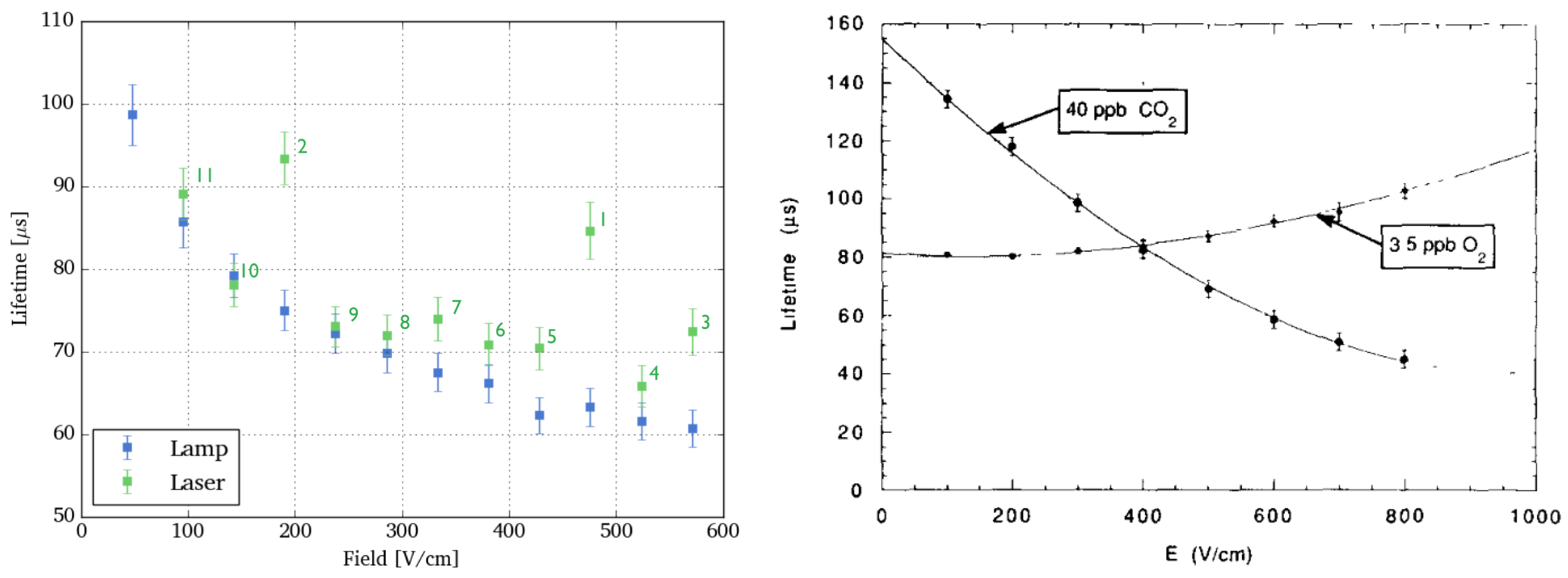
Figure 5.31: Left: Electron lifetime as a function of mean electric field. The first laser measurement was taken at t = 0 with following measurements taken at t = 12, 24, 36, 37, 40, 41, 44, 46, 48, 50 min. Measurements taken with the xenon flash lamp were taken in order with increasing field ranging from 56 - 77 min. Right: Electron lifetime dependence on the electric field in purified LAr as a function of different impurities [316].

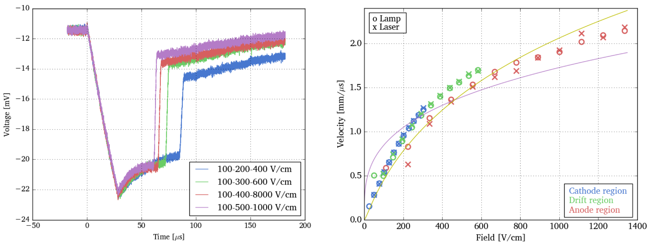
Figure 5.32: Left: Holding the field in the cathode region constant but changing electric fields in the drift and anode regions demonstrates the dependence of electron velocity on the electric field. Right: Electron drift velocity in LAr. Drift velocities can be obtained from all three regions of the purity monitor indicated by different colored markers. The purple line is a fit from [335] at 87.3 K, and the yellow line is a fit from [336] with parametrization at 85 K. Since electron velocity in LAr varies with temperature it is not expected that these fits will agree.

5.3.5.3 Electron velocity in liquid argon

Since the purity monitor can be operated at a wide range of electric fields, it can be used to measure the velocity of electrons in LAr as shown in Figure 5.32. Fits from [335, 336] are included for comparison. It is clear that the observed electron velocity is non-linear as a function of the field [337]. It has also been demonstrated that electron velocity in LAr varies with temperature [321] and the amount of impurities [338]. In fact, some of those experiments used detectors nearly identical to the purity monitor described here for their measurements.

5.3.6 Alternative design ideas

Initially, an alternative purity monitor design was pursued. Instead of generating electrons by the photoelectric effect on the cathode, a radioactive source with a PMT acting as a trigger was used. This would eliminate the need for the fairly expensive and impractical optical fiber needed to deliver light to the photocathode. This section describes the basic idea of this design, which was inspired by [339, 340, 341]. Unfortunately, due to the move to LBNL and with a tight deadline in sight in order to deliver a working purity monitor for the LZ HV feedthrough tests, the radioactive source design was abandoned due to the large amounts of R&D needed to get a working prototype.

A photograph of the original purity monitor is shown in Figure 5.33. A radioactive source located on the cathode creates ionization and scintillation signals as it decays. The ionization electrons drift through the purity monitor to the anode and constitute the signal seen on the oscilloscope. The scintillation signal is detected by the PMT and used as a trigger. As discussed in Section 5.1.3.1, the $128\,\mathrm{nm}$ scintillation light emitted in LAr is not visible to the bialkali PMT used (with a range of $\sim 300-600\,\mathrm{nm}$). Therefore, $0.11\,\mathrm{mg/cm^{3}}$ of TPB was deposited on a sheet of PTFE rolled inside the field cage re-emitting the light within the PMT range.

Two different sources were used for tests. ²⁰⁷Bi that decays to ²⁰⁷Pb with a half-life of 32.9 years. It emits 1 MeV internal conversion electrons 20% of times. However, light is also created by radioactive backgrounds, which makes triggering selectively on the stochastic radioactive decay complicated. Subsequently, ²¹⁰Pb source with a higher energy decay was used instead. It disintegrates to ²⁰⁶Pb via a 5.3 MeV $\alpha$ decay with a half-life of 138 days. However, neither option created a detectable PMT signal, likely because the radioactive source was located too far from the PMT. Therefore, radioactive background events near the PMT could create an overwhelming amount of triggers, flooding the signal from the ²¹⁰Pb decay and making it hard to detect.

A possible design improvement would be to relocate the PMT closer to the cathode to increase signal brightness and to improve trigger efficiency. This would require changing the cathode design to a grid to make it transparent to light. For example, an aqueous solution of ²¹⁰Pb could be deposited on wires as has been done in [342] and the TPB could be deposited directly on the PMT face. Alternatively, a transparent conductor, such as indium tin oxide (ITO) could be used. In this case, the TPB-coated PMT would be located directly behind the transparent cathode, looking into the purity monitor.

Ultimately, the advantage of the design that includes a radioactive source is the lack of a photocathode and the optical fiber which is delicate and can be impractical. Furthermore, if many feedthroughs are used between the light source and the cathode, this can lead to large losses of light. However, this problem can be avoided since a sufficient amount of light was delivered to the purity monitors developed in this work despite using three optical fibers connected by two feedthroughs.

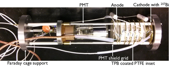
Figure 5.33: Photograph of the original purity monitor built at Yale University with ²⁰⁷Bi deposited on the cathode and a PMT serving as a trigger.

5.4 Purity monitor for XeBrA

A second purity monitor used in the XeBeA detector was built by Glenn Richardson, my undergraduate advisee at UC Berkeley. The design closely followed the purity monitor for LZ described earlier but features a few changes described here.

Purity monitor geometry	Value	Unit
Cathode & anode diameter	52.3	mm
Cathode - cathode shield grid	10.0	mm
Cathode shield grid - anode shield grid	70.0	mm
Anode shield grid - anode	5.0	mm
Cathode - anode	85.0	mm
Number of field shaping rings	6
Shield grids
Grid wire width	0.046	mm
Grid wire height	0.038	mm
Grid wire spacing	1.000	mm

Table 5.6: Parameters of the XeBrA purity monitor. The ground shield grid that serves to isolate the purity monitor from the main detector volume electrostatically has a pitch of 0.2 mm.

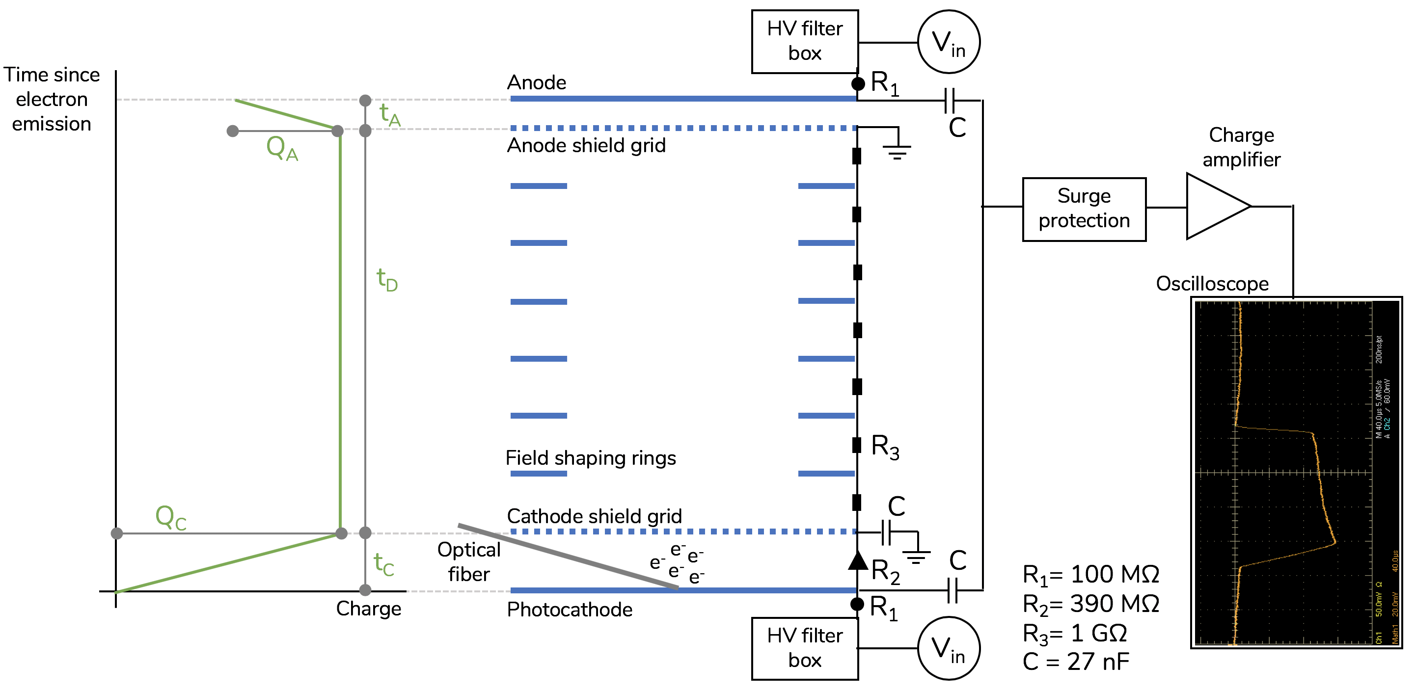
Figure 5.34: Schematics of the purity monitor deployed in XeBrA with a trace obtained in LXe.

First, instead of having an interchangeable photocathode disk, the entire copper cathode was coated in gold. The field shaping rings and the anode were made out of brass. To reduce outgassing, the three supporting rods were manufactured from PEEK and spacers were made from alumina ceramic. All shield grids were custom made by photochemical etching of T301 stainless steel. The cathode and anode grids were designed to ensure that doubling electric fields would result in 100% transparency for drifting electrons. The ground shield disk located at the end of the purity monitor serves as a Faraday cage to insulate the purity monitor from the rest of the experimental region. Table 5.6 includes a summary of the purity monitor parameters. The electronics were designed similarly to the LZ purity monitor but with the cathode, instead of the anode, biased to high voltage as shown in Figure 5.34. NPO type capacitors were used since their capacitance is not temperature dependent [322].

A photograph of the purity monitor is shown in Figure 5.35. The purity monitor was tested in LAr using the setup described in Section 5.3.2 and has been successfully operated in XeBrA in both LAr and LXe.

A third purity monitor that very closely follows the design of the XeBrA purity monitor is currently being built at LBNL to be used in the IBEX optical experiment.

Figure 5.35: Left: Photograph of purity monitor used in XeBrA. Right: The purity monitor is entirely contained inside CF flanges that also act as a Faraday cage. The optical fiber is delivered from the side. Since the cathode is at high voltage, it is conservatively designed to have a separate feedthrough.

5.5 Conclusion

The LZ detector is a two-phase xenon TPC currently under construction at SURF in Lead, South Dakota. The collaboration aims to start physics data collection in 2020. The LZ detector will probe a significant amount of the remaining parameter space above the neutrino floor for the direct detection of SI and SD WIMP-nucleus elastic scattering. Tests of various subsystems are ongoing at all of the collaborating institutions, and UC Berkeley is responsible for the cathode HV delivery. To validate results from the cathode HV feedthrough tests a purity monitor was successfully developed to provide a reliable and straightforward way to measure LAr purity in situ in real time. Due to the success of the LAr purity monitor a second purity monitor was built to monitor LAr and LXe purity in XeBrA, followed by a third monitor currently in development for the IBEX experiment.

5.5.1 Contributions to LZ

As a member of the LZ collaboration, I contributed to the cathode HV feedthrough development at Yale and LBNL by designing, building, and testing the purity monitor as described in this chapter. The purity monitor served an essential role in the high voltage feedthrough tests. I also assisted with the feedthrough tests themselves and optimized electric field models of an earlier version of the LZ feedthrough. Because of my experience modeling electric fields of the LUX detector, I advised a graduate student at UC Berkeley developing an axially-symmetric LZ field model used in data analysis.

I also spent time on site at SURF to assist with the installation of the radon reduction system used in the surface cleanroom where the LZ detector is being assembled. The radon reduction system was manufactured by the Ateko company based in Hradec Králové, Czech Republic [343]. I provided English-Czech translation and helped with safety training of the workers. The system has been shown to reduce the level of ²²²Rn in the air from $\sim 50\,\mathrm{Bq/m^{3}}$ by a factor of 1,000 [344]. Similar systems have been installed in Yangyang Laboratory in South Korea, Canfranc-Estacion in Spain, and in LNGS at Gran Sasso, Italy.

Furthermore, I founded the LZ Equity & Inclusion committee that has since become an integral part of the LZ collaboration. More details about the foundation of the committee and its activities are described in Appendix A.

Chapter 6 Xenon Breakdown Apparatus (XeBrA)

The goal of the Xenon Breakdown Apparatus (XeBrA) at the Lawrence Berkeley National Laboratory (LBNL) is to characterize the high voltage (HV) behavior of liquid xenon (LXe) and liquid argon (LAr). As will be discussed in this chapter, the probability of a dielectric breakdown increases for large electrode surfaces and depends on other factors, such as the noble purity. This is a concern, since as noble liquid detectors grow larger in size, achieving stable HV on the detector’s cathode becomes increasingly challenging. A breakdown in a two-phase TPC is a concern because it can damage detector hardware. Even before a full breakdown occurs, spurious light and charge emission can compromise detector performance at lower voltages. Therefore the results from XeBrA will not only improve our understanding of dielectric breakdown, but they will serve to inform the design of the next-generation noble liquid time projection chambers (TPCs).

The original measurements of liquid argon breakdown were done over micrometer gap distances [345, 315], skewing the community’s outlook on the plausible HV performance of the detectors. As larger detectors were developed, they were not able to reach the voltages predicted by these studies. Later measurements in LAr at more realistic centimeter scales revealed behavior pointing to electric field breakdown dependence on many variables such as electrode area, material, surface finish, LAr purity, and more. Due to the similarities between LAr and LXe, this behavior is likely also to be seen in LXe. However, there is a relative lack of such measurements in LXe.

HV behavior in liquid nobles is only beginning to be explored, but there have been studies of dielectric breakdown behavior in other media. Section 6.1 provides a brief overview of selected studies and identifies trends that may be of interest to study with XeBrA. Dependence of breakdown on electrode area has been widely agreed upon in the community; however, a theoretical explanation of the process has still not been identified. So far, the best answers have arisen from extreme value (weak link) theory discussed in Section 6.2. It should be noted that breakdown dependence on electrode size is not a unique effect: there are many products whose failure rates are often assumed to be proportional to their size. Some examples include capacitor dielectric (proportional to area), cable insulation (proportional to length), electrical insulation (proportional to thickness), and conductors in microelectronics (proportional to length and number of bends) [346].

The initial studies in XeBrA were focused on exploring the area effect. The largest measured area in the literature achieved in LAr is only $3\,\mathrm{cm^{2}}$, limited by the geometry of the electrodes. To overcome this limitation, XeBrA utilizes Rogowski electrodes optimized for field uniformity over large areas (Section 6.3.1.1); thereby providing insight into areas that are more relevant to the large experiments. Additionally, XeBrA can be filled with either LAr or LXe and can test electrodes with areas up to $58\,\mathrm{cm^{2}}$ by varying their separation remotely. This makes XeBrA the first apparatus to enable a direct comparison of HV behavior between LAr and LXe, providing new insight into HV behavior in noble liquids useful in both dark matter and neutrino detection. The design of the apparatus is detailed in Section 6.3, and HV considerations for optimizing the main liquid volume to ensure breakdown occurred between electrodes are discussed in Section 6.3.1.

There is a purity monitor (Section 6.3.2) and a PMT (Section 6.3.3) directly adjacent to the main active volume. The purity monitor measures the electron lifetime, which provides information about the liquid purity. The PMT is used for the study of the onset of electroluminescence. Additionally, two current monitor devices are attached to the anode. Along with the PMT, they serve to look for signs of early breakdown development prior to the formation of the spark. If a predictive pattern could be identified, then breakdowns in future detectors could be prevented by stopping the HV ramp in a timely manner.

A dedicated gas system was designed and built to be shared by XeBrA and IBEX. Its development is described in Section 6.4, and a procedure developed for its operation is included in Appendix C. There are two more Appendices related to XeBrA included in this work. Appendix B serves as a brief introduction to the various types of fittings used in the construction of both the apparatus and the gas system mentioned throughout the text. The fittings appendix can also serve as a general reference for anyone building a system for handling noble gases. A list of parts used both in the gas system and in XeBrA is included for completeness, and can be found in Appendix D.

Section 6.5 discusses XeBrA operations, and Section 6.6 provides an overview of the four data acquisitions made during 2018: two made in LAr and two in LXe. The analysis of these data along with preliminary results is presented in Section 6.8. A publication of results from the 2018 scientific operation is in preparation. Looking ahead, Section 6.9 includes a discussion of future studies for which XeBrA would be suitable.

6.1 Breakdown studies primer

There are no published comprehensive studies of dielectric breakdown behavior for large area electrodes in LXe. These measurements are desirable not only to improve our understanding of the physical processes involved in the breakdown but also to inform the future of TPC engineering. These are the primary motives for XeBrA. However, the dielectric breakdown has been of interest for many decades in various other materials due to their application as insulators in electric power generation and transmission. This section provides a brief overview of the literature for selected materials and highlights relevant effects that might be of interest in LXe. Studies of dielectric breakdown as a function of both alternating current (AC) and direct current (DC) are available in the literature, and the breakdown behavior appears to vary between AC and DC. Only DC HV is currently of interest for LXe detectors, which dictates the focus of this primer.

All studies agree that dielectric breakdown depends on the electrode area with high electric fields. This dependence can be justified experimentally, although a simple thought experiment can provide good intuition about the effect [347]. A sketch of the thought experiment is as follows. Assume that breakdown for a given area $A_{0}$ is measured and the breakdown field $E_{0}$ is found as the mean of $N$ measurements. Consider an experimental apparatus consisting of $n$ copies of the $A_{0}$ experiment connected in parallel, resulting in a larger area $A=n\times A_{0}$. A single data point can be generated for the apparatus with area $A$ by taking the minimum of a random selection of $n$ data points from the original experiment. Repeat this random sampling $m=N/n$ times to generate a full dataset, ensuring subsequent choices are disjoint. The mean of this new dataset will represent the dielectric breakdown for an area $A$. This mean (since it is a mean of minima) will be less than $E_{0}$, the mean of the $A_{0}$ experiment. This justifies that larger areas result in dielectric breakdowns at lower electric field values. This effect is also known as the stability postulate in probability theory, which is leveraged in the weak link theory.

Transformer oil

Transformer oil is commonly used for its excellent electrical insulation properties. Most tests in transformer oil were made using AC. Several studies observed decreasing breakdown performance with increasing electrode area using Rogowski electrodes of multiple sizes [347, 348]. Impurities in oil increased the chance of breakdown, and the breakdown values depended on the velocity of contaminants moved by oil circulation [349]. Dependence of breakdown on the oil volume subject to high electric stress was observed as well.

Liquid nitrogen

Reference [350] observed an area effect using multiple parallel plate electrodes. The study also notes that dielectric breakdown occurred at lower voltages in the presence of small bubbles. Reference [351] observed that increasing electrode area and stressed volume, having a mutual correlation, decreased HV performance (sphere to plane electrode geometry). Electrode polarity was also observed to affect breakdown values.

Liquid helium

Extensive studies have been performed in liquid helium (LHe) for applications in neutron electric dipole moment searches [352, 353, 354, 355]. Reference [356] contains a comprehensive review of breakdown test conditions in LHe to that date. Reference [292] identified dependence of dielectric breakdown on electrode area and spacing, liquid purity, electrical field conditions, test procedure, liquid pressure and temperature, and electrode surface condition. The surface roughness of the cathode was identified as the most critical parameter [292]. Addition of oxygen or conducting impurities had an adverse effect on breakdown strength, as dirty LHe was observed to break down at lower fields. Bubble formation occurred during any breakdown in LHe [292, 357]. Additionally, bubbles were found to cause breakdown due to their lower dielectric strength. A polarity effect was observed [357], with the breakdown initiated on the cathode [292]. Reference [356] observed a volume power law when considering only the half of the stressed volume adjacent to the cathode.

Liquid argon

There are abundant studies performed in liquid argon (LAr) for applications in neutrino interaction and oscillation experiments. One of the first available studies in LAr used 5 mm diameter electrodes with varying separations and tested six different electrode materials that were observed to affect the dielectric breakdown behavior [315]. An effect of material oxidation was observed as well. Based on the limited sample size of that study, stainless steel (SS) performed the best. Reference [315] also observed an increase in breakdown strength with higher oxygen impurity concentrations (an effect opposite to what was observed in LHe). The effect of impurities was later confirmed by [358] as shown in Figure 6.1. Reference [358] also confirmed that the location of sparks varied for consecutive sparks. Using Rogowski electrodes for their studies, Reference [359] confirmed that LAr bubbles worsen the breakdown performance.

Figure 6.1: A comparison of various measurements performed in liquid argon as a function of electrode separation. Dependence of breakdown on purity can be seen. Additionally, larger electrodes were observed to perform worse than smaller ones at a given electrode separation. Figure from [358].

There were two notable efforts in recent years to investigate breakdown behavior in LAr. One was at the Laboratory for High Energy Physics (LHEP) at the University of Bern, Switzerland [360, 314, 313]. Measurements at LHEP were performed at $\sim 1.2\,\mathrm{bar}$ [314], using SS electrodes with mainly a mechanical polish of $0.1-0.4\,\mathrm{\mu m}$. Their studies confirmed the area effect. They also managed to suppress the field emission using an emulsified water solution to deposit a layer of natural polyisoprene (latex rubber) onto the cathode surface. However, the performance of the coating degraded and became very similar in performance to SS electrodes after the first breakdown that damages the rubber. They also monitored spark development using a camera and a spectrometer leading to a detailed description of breakdown development.

The other effort was at the Fermi National Accelerator Laboratory (FNAL). Measurements there were taken at $1-1.6\,\mathrm{bar}$ [358]. Their electrodes were polished to a mirror finish, then electropolished, but the exact value of the electrode finish is not known.

Liquid xenon

There is one published study in LXe performed at SLAC [361] as part of the EXO-200 experiment [197]. The setup used two 1.5 cm diameter spheres separated by 1 mm for the measurement with area $3.1\,\mathrm{mm^{2}}$ ($0.031\,\mathrm{cm^{2}}$ ) reaching 90% of the maximum electric field. Breakdowns were observed at $250-300\,\mathrm{kV/cm}$. Neither the purity nor the pressure at which the data point was obtained is known.

Figure 6.2: Simulation of electric fields around the cathode of the LZ detector. The inner cryostat wall is located to the left of the picture. The outer diameter of the cathode frame is 150 cm. The turquoise arrow indicates the point with the highest field (26 kV/cm) on the cathode frame. The red arrow indicates the highest electric field in the field cage (29 kV/cm), located on the reverse field region (RFR) ring. Figure from [362].

The stressed area in LZ will be much larger than what was studied at SLAC. According to simulations and assuming -100 kV on the cathode, the highest electric field in the LZ field cage is on the field shaping ring directly below the cathode, in the reverse field region, as shown in Figure 6.2. The electrode area with a field equal to or larger than 90% of the maximum field (29 kV/cm) corresponds to $150\,\mathrm{cm^{2}}$. The largest area at high voltage is the cathode frame, with a maximum field of 26 kV/cm over an area of $500\,\mathrm{cm^{2}}$. The LZ electrodes are manufactured from 304 SS.

6.1.1 Summary of parameters affecting breakdown behavior

The adverse effect on dielectric breakdown caused by increasing electrode area has been agreed on in studies in many materials. However, other effects have been identified to influence dielectric breakdown behavior. A list of some of these effects with references to the relevant literature follows.

• Area: The most universally agreed upon factor affecting breakdown behavior. See for example [347, 348, 350, 351, 356, 292, 358, 314, 363, 364, 365].

• Volume: Some studies also report breakdown strength decrease with an increase of the stressed liquid volume [351, 356, 363, 364].

• Surface finish: Smoother finish has been shown to break down at higher voltages in LHe [356, 292] and in LN [351].

• Material: Varying materials, as well as surface oxidation, affected dielectric breakdown in LAr [315]. Material dependence was also observed in LHe [356, 292].

• Pressure and temperature: Breakdown performance improved with increasing pressure in LN [350] and LHe [292, 354]. However, Reference [350] notes that earlier studies in LN saw a decrease in breakdown values with increasing temperature (which is directly correlated with pressure).

• Purity: Impurities increased the chance of a breakdown in transformer oil [349] and LHe [292]. However, in LAr, the presence of impurities improved HV performance of the experimental setup [315, 358, 313].

• Polarity: It is believed that the spark during a dielectric breakdown is initialized on the cathode surface and affected by space charge effects on the cathode surface and in the stressed volume [358, 313]. Previously, the effect of polarity was observed in a vacuum where the breakdown performance was worse when strong fields were applied to the cathode rather than the anode [365]. The same behavior was also observed in LN [351] and LHe [292, 357].

• Conditioning: Conditioning is frequently used in vacuum applications to increase the breakdown voltage of surfaces. Applying high electric fields to critical regions serves to burn off impurities and surface irregularities that might act as field emission sites during breakdown otherwise. Note that this is only the case if the current is not high enough to damage the electrodes. However, the effect of conditioning electrode surfaces is unclear in liquid nobles. It appears to be a valid mechanism in a vacuum, particularly with impulse voltage [365, 366, 367] and transformer oil [349], but its effects are uncertain in LHe [292, 368].

• Circulation speed: Breakdown voltage in transformer oil has been shown to depend on circulation speeds. The impact on breakdown varies at various velocities [349].

• Capacitance: References [369, 370] have argued that a decrease in dielectric strength in a vacuum can be caused by changes in the energy stored in the system. They observed that a capacitor placed in parallel with the electrodes reduces dielectric strength (and also makes electrode damage more significant).

This section does not attempt to provide an exhaustive list of parameters affecting breakdown behavior in liquids. XeBrA’s construction and design allow for all of these parameters to be explored in the future, for both LAr and LXe.

Aside from identifying trends caused by dielectric breakdown, the physics of the initiation of dielectric breakdown and the succeeding discharge evolution also remains a mystery.

There are two leading plasma-initiating mechanisms in water. One, the electronic mechanism, considers electrical discharge to be generated purely by ionization followed by electron multiplication, only later followed by a bubble. The other one, the bubble mechanism, assumes that plasma initiation occurs in the gas phase, in the naturally present nanobubbles. Characterizing this behavior is an active field of research, but there is no universal agreement so far. The answer likely depends on the precise experimental parameters. Reference [371] provides an excellent overview of the state of the plasma physics of liquids to date.

6.2 Review of statistical analysis of area effects

Extreme value theory aims to find a probability of more extreme events than previously observed. A thorough introduction to the topic is, for example, in [372]. It is commonly applied in engineering to predict failures of products based on a small tested sample, in hydrology to assess likelihoods of 100-year floods, or in traffic prediction. Also known as weak link theory, in application to dielectric breakdown it is expected that continuously increasing the area or volume subjected to stress will increase the probability of finding a weaker link causing a breakdown. These weak links are presumed to be particles, active emission sites on electrodes, or surface irregularities. For extreme value theory to be applicable, there should be a substantial number of flaws distributed at random and independently. Additionally, any statistical model used to describe this behavior should follow the stability postulate.

An early application of extreme value theory to breakdown probability in materials (and many other real-life applications) was demonstrated in [373, 372]. Several cumulative distribution functions satisfy the stability postulate in the extreme value theory field, such as Fréchet, Weibull, or Gumbel functions; Gumbel and Weibull distributions have been widely used in the field, but the Weibull function is particularly popular since it is commonly used in reliability engineering. The Weibull function is a special case of the generalized extreme value distribution. Representing the breakdown probability as a 2- or 3-parameter Weibull function takes one of the forms:

$$p= 1-e^{\left(\frac{x}{\lambda}\right)^{k}}$$ (6.1)

$$p= 1-e^{-\left(\frac{x-\theta}{\lambda}\right)^{k}}$$ (6.2)

for $x\geq 0$ where $x$ is a random variable (breakdown voltage or field), $k>0$ is the shape parameter, $\lambda>0$ is the scale parameter, and $\theta$ is the location parameter of the distribution. For $\theta=0$, Equation 6.2 reduces to the 2-parameter Weibull distribution in Equation 6.1. The shape parameter $k$ is correlated to the stressed area as

$$A=\underset{S}{\iint}\left(\frac{E_{i}}{E_{max}}\right)^{k}dS$$ (6.3)

where $E_{i}$ is the electric field at an individual unit on the surface of an electrode and $E_{max}$ is the maximum electric field and $dS$ is the area differential [374]. The authors of [374] show that the 3-parameter Weibull distribution is a good method for approximating breakdown stressed area in transformer oil.

From the 2-parameter Weibull function, assuming the stability postulate, a general power law for an area effect can be derived

$$E_{max}=E_{0}\left(\frac{A}{A_{0}}\right)^{-\nicefrac{{1}}{{k}}}$$ (6.4)

where $A_{0}$ is a hypothetical unit area, and $E_{0}$ is the electric field that breaks down at that area. Note that $E_{0}$, $A_{0}$, and $k$ are all constants in this formula. This formula has been simplified further and is commonly used to fit the area effect (and the volume effect):

$$E_{max}=C\times A^{-b}$$ (6.5)

where $b=1/k$.

Furthermore, if the breakdown distribution at area $A_{0}$ is known, the mean $E_{0}$ may either be computed directly from the sample or calculated as the analytical mean of the fitted Weibull function. Equation 6.4 then becomes

$$E_{max}=\lambda\Gamma\left(1+\frac{1}{k}\right)\left(\frac{A}{A_{0}}\right)^{-\nicefrac{{1}}{{k}}}$$ (6.6)

and can, in theory, be used to attempt to predict breakdown behavior as is done in Section 6.8.6. Here $\Gamma\left(x\right)$ is the gamma function. Moreover, the weak link theory predicts that the location of sparks will vary for each breakdown.

Reference [375] demonstrated that the scale parameter of the Weibull function decreases as a function of electrode area, confirming the area effect for AC studies in oil. They also demonstrated that the shape parameter of the Weibull distribution is independent of the stressed area of the electrode and instead is a constant determined by the liquid type. The weakest link theory has also been applied to breakdown in LHe [364, 376, 377], LN [347, 363, 378, 379, 380], alumina [381], polymer films [382], and more [383, 384]. Further refinement and applications of these statistical techniques of data generated by XeBrA is a promising area of future study with the apparatus.

6.3 Apparatus design

The goal of XeBrA is to study HV behavior in LAr and LXe. The apparatus design was optimized to use the largest possible electrode areas inside a given volume. All parts were chosen after deliberate considerations as outlined below and all parts submerged in LXe were selected to minimize the amount of impurities they will release into the LXe. Overview of the detector is shown in Figure 6.3.

XeBrA uses $\sim 16\,\mathrm{kg}$ of LXe. Practical considerations limited the amount of xenon: the apparatus is expected to enable multiple measurements while varying parameters between data acquisitions, so it is vital that xenon condensation, cleaning, and recovery take at most a few days. For comparison, an apparatus with 250 kg in the active volume, the size of LUX, requires months to condense and clean the xenon. On the other end, a detector that is too small does not make it possible to probe dielectric breakdown over large areas. This optimization led to a selection of a 6-inch stainless steel spherical square vacuum chamber from Kimball physics, shown in Figure 6.4, as the central part of the apparatus. The spherical square used in XeBrA was modified and includes one 8-in CF, one 6-in CF, four 4.5-in CF, and eight 1.33-in CF ports.

Figure 6.3: Modified spherical square used in XeBrA with annotated ports. Its spherical inner diameter is 149.86 mm (5.90 inches) with an internal volume of $2028\,\mathrm{cm^{3}}$.

Figure 6.4: Annotated CAD rendering of XeBrA.

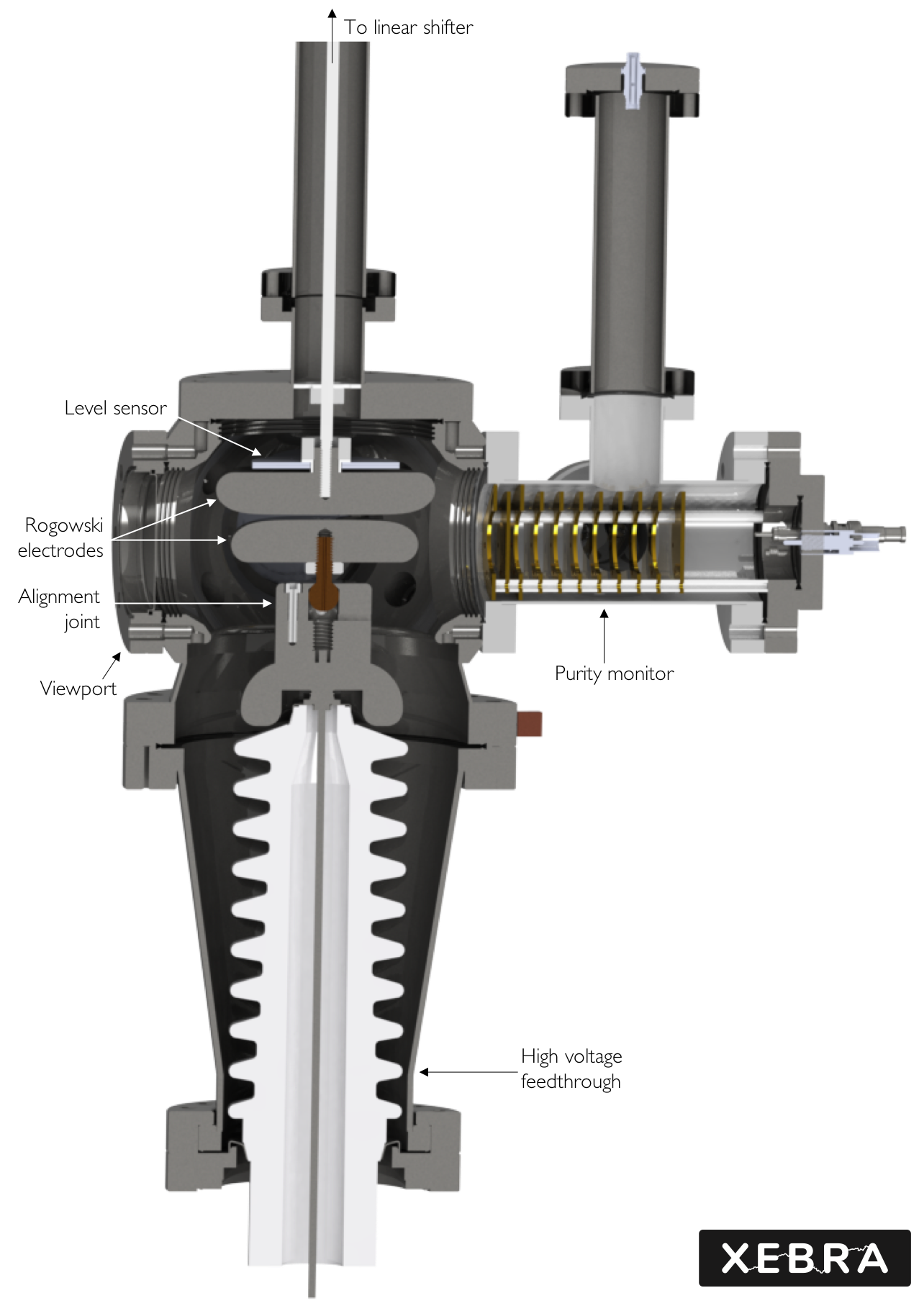
Figure 6.5: CAD rendering of the active volume of XeBrA. The level sensor is fastened to the top electrode. The PMT is not visible.

Measurements were performed using Rogowski electrodes to maximize the electrode area. The Rogowski electrodes, discussed in Section 6.3.1.1, were located in the center of the spherical square as shown in Figure 6.5. The top electrode was at 0 V and attached to a linear shifter that changed the separation of the electrodes. The bottom electrode was connected via an alignment connector to an HV feedthrough as discussed in Section 6.3.1.2. Two of the 4.5 in CF ports were used as viewports; a purity monitor (Section 6.3.2) and a PMT (Section 6.3.3) were attached to the other two ports. On top, the spherical square attached to the top flange of the outer vessel (OV) via a CF nipple to create vertical clearance for the heat exchanger. The OV was evacuated for thermal insulation as described in Section 6.3.4. The apparatus was cooled through a heat exchanger attached to a pulse tube refrigerator (PTR) as specified in Section 6.3.5.

6.3.1 High voltage design

Along with electric fields, a key quantity of interest is the stressed cathode (or electrode) area (SEA). In this work, the SEA is defined as the area of the cathode surface with an electric field magnitude exceeding 90% of the maximum electric field, as illustrated in Figure 6.6. The radius was obtained from simulations in COMSOL Multiphysics v5.0^® [259]. The stressed area was calculated assuming that the Rogowski electrodes are perfectly flat within the region of interest. The choice of 90% SEA was influenced by recent studies done in LAr [314]. However, most breakdown values reported in the literature define SEA as either 80% or 90% of the maximum electric field. Reference [363] found that 80-85% SEA was appropriate (in LN), while a more recent work of Reference [374] found that Weibull distribution corresponded to 90% of the electrode surface (in transformer oil).

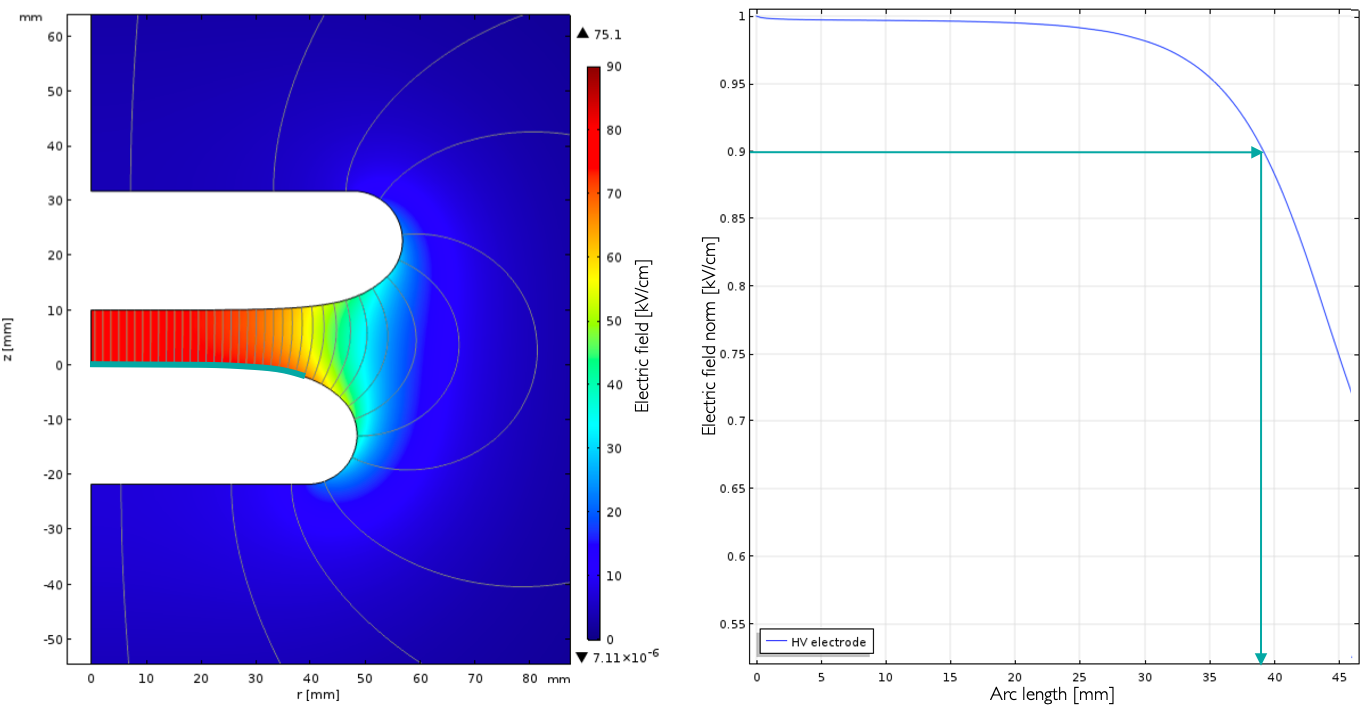
Figure 6.6: Illustration of cathode stressed area. Left: Electric field between two Rogowski electrodes. The teal line illustrates the arc length along the cathode surface where the electric field magnitude is being evaluated. Right: Plot of the electric field for the setup on the left normalized to the maximum electric field. The teal arrows illustrate 90% of the maximum field.

6.3.1.1 Rogowski electrodes

Previous experiments in LAr have used a grounded flat plane as one electrode and spheres of varying diameters as the second electrode. These setups do not achieve very large electrode stressed areas. Instead, XeBrA uses Rogowski electrode profiles, as calculated in [385]. Originally conceived by W. Rogowski [386], the Rogowski equipotential lines in a gap formed by a finite plane above an infinite ground plane are given by

$$\begin{cases}x=\frac{d}{\pi}\left(\phi+e^{\phi}\cos\psi\right)\\ y=\frac{d}{\pi}\left(\psi+e^{\phi}\sin\psi\right)\end{cases}$$ (6.7)

where $\psi\in\left[0,\pi\right]$ is the equipotential surface, $\phi$ is the line of electrostatic force and $d$ is the distance between the plane electrode and the infinite ground plane. This expression can be obtained via a conformal mapping in complex analysis [387]. The values of $\phi\in\left[-\infty,\infty\right]$; for $\phi\rightarrow-\infty$, the expression approaches a constant, corresponding to the center of the electrode. For $\phi\rightarrow\infty$, the expression diverges. The effect of varying $\psi$ is illustrated in Figure 6.8.

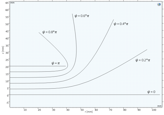
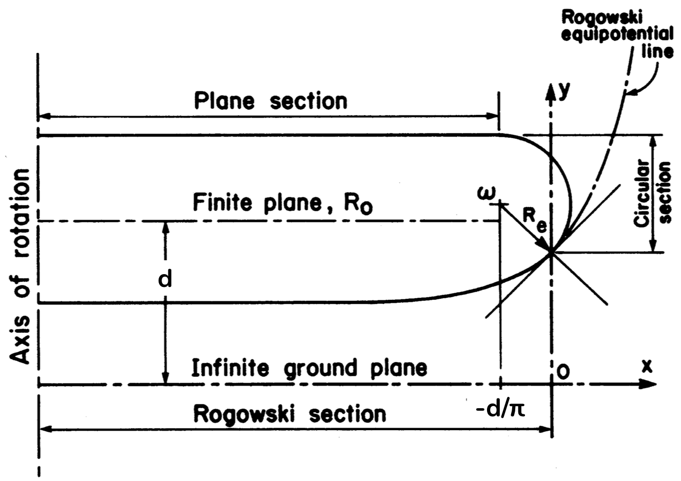
Figure 6.7: Equipotential lines for a finite plate 2 cm above an infinite ground plate illustrating different values of $\psi$.

Figure 6.8: Rogowski electrode profile with $\psi=\pi/2$. Figure modified from [385].

The conventional Rogowski profile corresponds to an equipotential surface at $\psi=\pi/2$. This choice was verified experimentally to impede arcing at the edges of the electrodes. This simplifies Equation 6.7 to

$$\begin{cases}x=\frac{d}{\pi}\phi\\ y=\frac{d}{\pi}\left(\frac{\pi}{2}+e^{\phi}\right)\end{cases}$$ (6.8)

and results in the Rogowski equipotential line shown in Figure 6.8. To manufacture such an electrode, it is necessary for the electrode to be finite. A circular section can be used to terminate the electrode. The calculation leading to the design shown in Figure 6.8 used in XeBrA can be found in [385]. Since the electrode needs to be enclosed inside of a grounded vessel, it is also important to consider electric field interactions between the electrodes and the vessel. Field enhancement due to the proximity of a grounded wall begins when the radial distance separating the electrode from the vessel is about twice the main gap spacing.

Conveniently, the shape of the electrodes depends only on $d$, the separation between the electrodes, rather than on their potential difference. If two Rogowski electrodes are used, the electrode thickness should be twice the maximum gap space $d$ to avoid excessive field enhancement at the electrode edges. This fully defined the electrode design. Therefore, electrodes with 2 cm thickness can be used to study electrode areas up to $58\,\mathrm{cm^{2}}$ with up to 1 cm electrode separation. Since it is challenging to ensure that the two electrodes are perfectly aligned, the ground electrode (anode) was manufactured with a slightly larger radius ($r=56.6\,\mathrm{mm}$) compared to the HV electrode (cathode) with $r=48.4\,\mathrm{mm}$. The slightly larger size of the ground electrode ensures that if the two electrodes are somewhat off-axis, all the electric field benefits of Rogowski design would be maintained. The maximum size of the HV electrode was determined from HV simulations in COMSOL constrained by the size of the spherical square used. The electrodes were manufactured from 303 stainless steel. The cathode had a surface finish with roughness average (Ra) of $0.05\,\mathrm{\mu m}$ and anode with $\mathrm{Ra}=0.07\,\mathrm{\mu m}$.

Figure 6.9: Effect of electrode tilt on electric field obtained from an axially symmetric simulation performed in COMSOL. The simulation was made in LXe for a 3 mm electrode separation with a 1^∘ tilt.

Separation [mm]	Nominal field [kV/cm]	Max field at 0.4∘ tilt	% increase from nominal field	Max field at 1∘ tilt	% increase from nominal field
1.0	750	789	5	957	28
1.4	536	555	4	634	18
2.0	375	385	3	421	12
3.0	250	254	2	270	8
4.0	188	190	1	199	6
5.0	150	152	1	158	5
6.0	125	126	1	131	5
7.0	107	108	1	111	4

Table 6.1: Effects of electrode tilt.

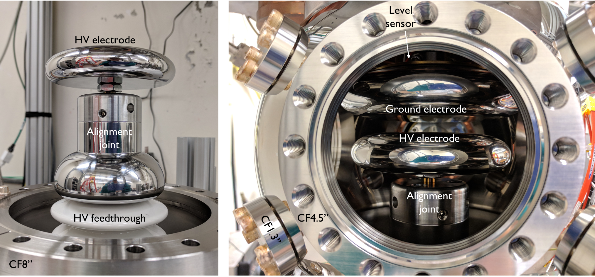
Figure 6.10: Image of the HV assembly. Left: Image of the HV electrode attached via the alignment joint mounted on top of the Ceramtec feedthrough. Right: Image of the assembly inside the spherical square.

A pressure recording film was used to align the electrodes to ensure that they are parallel inside the apparatus. Nevertheless, it is possible that the electrodes will be tilted with respect to each other. A COMSOL simulation was performed to study the effects of a 0.4^∘ and 1^∘ tilt as summarized in Table 6.1. A 1^∘ tilt would be clearly visible as illustrated in Figure 6.9. Based on a perception study, a 0.3^∘ tilt would be visible by eye in the setup. Since there are two directions of possible tilt, this results in a 0.4^∘ systematic error.

6.3.1.2 HV feedthrough connection

The HV electrode was attached to an alumina ceramic feedthrough made by CeramTec (model 6722-01-CF), rated up to 100 kV of 6.5 A DC in vacuum. The connection of the HV electrode to the feedthrough was carefully designed to ensure that the electric fields caused by this connection did not exceed the electric field expected between the electrodes. A special connector was designed with its dimensions optimized in COMSOL, and its implementation was engineered at LBNL. The resulting alignment joint is shown in Figure 6.10. The alignment joint served two purposes. First, it served as an HV connection between the HV electrode and the feedthrough. The radius of the bulge at the bottom of the joint was designed to minimize the high electric fields present at this interface. Second, a ball spindle located near the top of the joint allowed the electrodes to be aligned to be parallel to each other once inside the apparatus.

The final simulation of the electric field inside the active volume is shown in Figure 6.11. The DC dielectric constant of liquid xenon is assumed to be 1.85, which is typical of measured values in the scientific literature [388, 389, 390, 391]. The dielectric constant of alumina ceramic was set to 9.4.

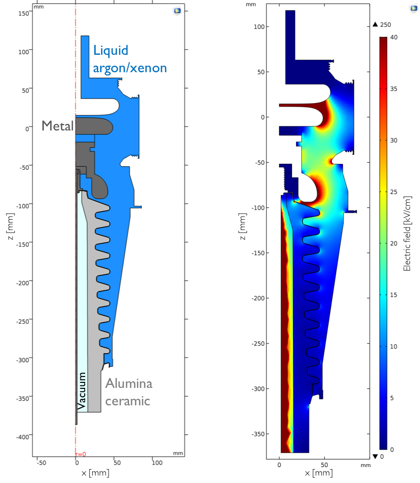
Figure 6.11: An axially symmetric simulation of the active volume of XeBrA performed in COMSOL. Left: Illustration of the geometry and materials used in the simulation. Right: Results of an electric field simulation in LXe with -75 kV on the cathode (bottom electrode). Maximum field occurs between the two electrode faces. At 5 mm electrode separation, the maximum field between the electrode faces is 150 kV/cm, while the second highest field in the apparatus (54 kV/cm) is at the rounded part of the alignment joint.

A power supply was purchased from Spellman (model SL100N10/CMS/LL20) with a range up to -100 kV with $100\,\mathrm{\mu A}$ DC. This power supply was previously tested for its stability and is very similar to the power supply used in the LZ detector. To comply with the Lab’s Environment, Health & Safety (EH&S) radiation regulations, the power supply was limited to -75 kV during operations with a maximum current of $10\,\mathrm{\mu A}$. The power supply can be controlled either manually or remotely through LabView in the Slow Control.

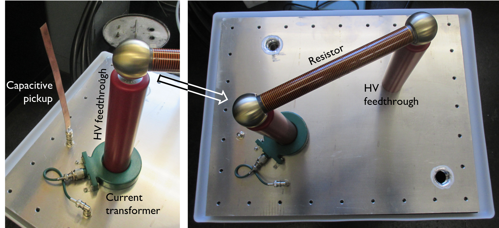
Figure 6.12: Electronics of the oil tank attached to an upside down lid. The parts are submerged in transformer oil during operations. Left: Current transformer and capacitive pickup next to one of the HV feedthroughs made by Isolation Products. Right: A $956\,\mathrm{k\Omega}$ resistor attached to two HV feedthroughs.

A $956\,\mathrm{k\Omega}$ resistor is installed between the power supply and the apparatus as shown in Figure 6.12 to limit the current and minimize the stored energy that can go into a breakdown. The resistor isolates the load from the stored energy in the power supply and some of the cable, which limits the amount of potential damage caused by a spark. The stored energy that is in the cable connecting the oil tank to the HV feedthrough will go into the breakdown. The resistor is located inside an oil tank instrumented with a current transformer to identify very large events and a capacitive pickup that can be connected to an oscilloscope. The capacitive pickup can detect a change in voltage as a result of a partial discharge or a full breakdown. If the HV were to break down to this pickup, a box with a spark gap to ground limits the signal level to 150 V at the output. Two HV feedthroughs (custom-made model D-102-10 from Isolation Products) are used to make the connection in the oil. They are rated to 100 kV DC and made from cast epoxy.

A cable (Dielectric Sciences model 2121) is used to connect the power supply, the oil tank, and the apparatus. The center of the cable is made from gauge 12 AWG tin-plated copper surrounded by semiconductive polyethylene. The conductive core is enclosed by low density high molecular weight (LDHMW) polyethylene. The cable is rated to 150 kV DC with a capacitance of 29 pF/ft. The total length of the cable between the oil tank and the apparatus is 2.1 m (7 ft), resulting in

$$E=\frac{1}{2}CV^{2}=0.6\,\mathrm{J}$$ (6.9)

of stored energy at -75 kV.

6.3.2 Purity monitor

Very high purity levels are desired for noble liquids in XeBrA for two reasons. First, the breakdown field strength is expected to depend on the presence of impurities in the liquid. Second, the results from XeBrA should inform direct dark matter and neutrino experiments, which typically operate at very high purities. To that end, a purity monitor capable of detecting very low levels of impurities was built to serve inside the XeBrA experiment. For more details about the design, development, and operating principles of the purity monitor, refer to Section 5.4.

The purity monitor was directly connected to the active volume as shown in Figure 6.15. It was mounted to one of the 4.5 in CF ports of the spherical square as shown in Figure 6.5.

An anode signal was never seen in the purity monitor while operating in LXe. A similar problem was observed during the construction of the IBEX purity monitor. It was discovered that the alumina ceramic spacers likely had small amounts of conductive impurities on their surfaces, making them slightly conductive. The ceramic spacers separating the anode and anode shield grid are the shortest so the number of lost charge would be most pronounced around the anode. Even though the purity monitor was operated successfully in LAr, it is anticipated that this effect was also present. It is possible that either this effect is temperature dependent or the purity achieved in LAr was higher than that of LXe, and the anode detected some of the charges. If this is true, then the purity of LAr reported in this work presents a lower limit on the electron lifetime, since some of the drifting electrons would not have been detected. Disassembly of the purity monitor and thorough cleaning of the ceramic spacers is planned before future operations.

6.3.3 PMT

As discussed in Section 5.1.2, one of the concerns of dual-phase LXe detectors is light production before a dielectric breakdown. Therefore, a PMT was installed to monitor the onset of electroluminescence prior to a breakdown. Similar to the purity monitor, the PMT is mounted to one of the 4.5 in CF ports of the spherical square adjacent to the active volume.

Electroluminescence is different for LAr and LXe, so two different PMTs were used for the two liquids. Each PMT was mounted inside a 4.5 in CF nipple so the entire assembly could be easily replaced between data acquisitions with different liquids. When collecting data with the PMT, the two viewports located on the OV are covered, making the active volume light tight. Then the cathode HV is slowly ramped up to a voltage that is very unlikely to result in a spark for a given electrode separation. The voltage is held constant for a few minutes, before being slowly ramped back down to the ground. Data are collected throughout the entire procedure to observe the onset of electroluminescence.

Note that the base for the PMT was designed to have low capacitance. Even though the PMT is not expected to be biased during breakdowns, if an unanticipated spark happens during PMT operations, this small capacitance should prevent PMT damage. However, the increase in the dark rate on the photocathode would likely last several hours at XeBrA’s operating temperatures preventing further data acquisition. The PMT bases were manufactured by Sunstone Circuits using Roger400x boards to minimize outgassing. Schematics of the printed circuit boards (PCBs) used for each PMT shown in Figure 6.13, as designed by Quentin Riffard, a postdoctoral researcher at LBNL.

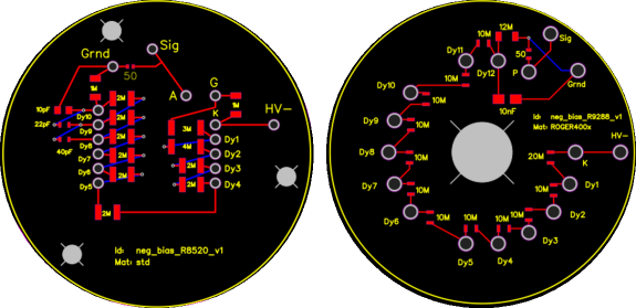
Figure 6.13: Schematics of PCBs used for PMT operations. Connections to the PMT dynodes are indicated by “Dy.” Right: For LAr PMT. Left: For LXe PMT.

6.3.3.1 Liquid argon PMT

For operations in LAr, a bialkali PMT from Hamamatsu (model R8520-06) was installed as shown in Figure 6.14. It has an effective area of $\left(20.5\times 20.5\right)\,\mathrm{mm^{2}}$ and a spectral response ranging from 160 to 650 nm. Tetraphenyl butadiene (TPB)-coated quartz disc was installed in front of it facing the active volume to wavelength-shift the 128 nm LAr scintillation light to 430 nm, a wavelength detectable by the PMT with high quantum efficiency.

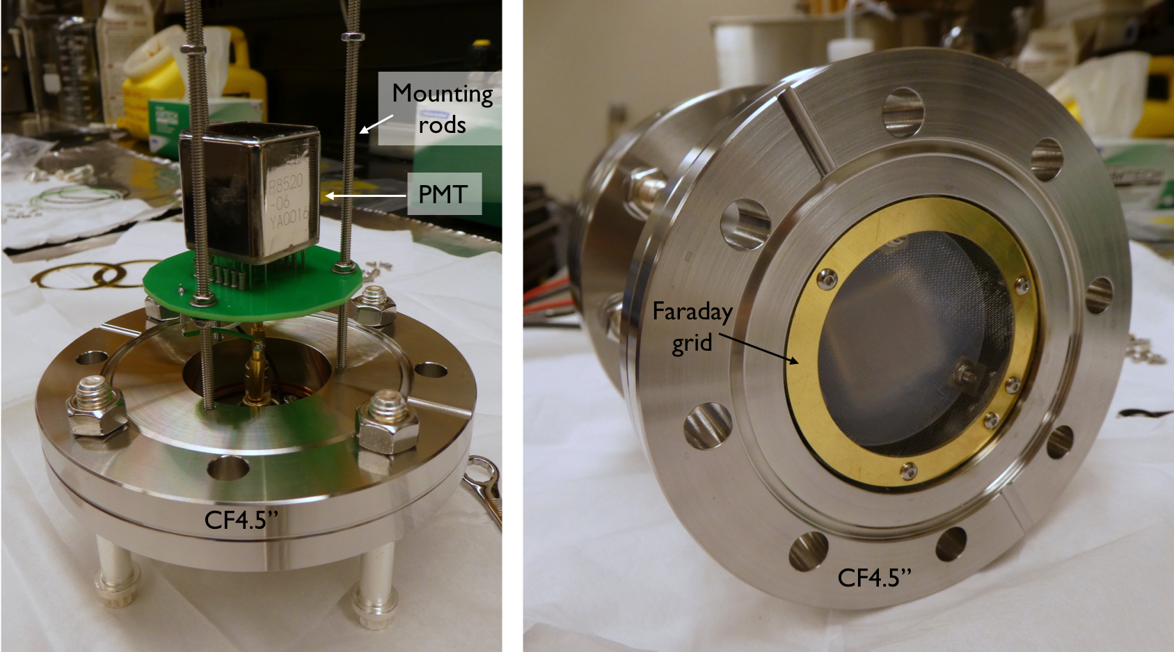
Figure 6.14: Pictures of the PMT assembly used in LAr. Left: PMT mounted on a CF4.5” flange. Right: View of the PMT inside the CF4.5” nipple. The Faraday grid at the forefront electrostatically separates the PMT from the active volume. Faintly visible just behind the grid is a TPB-coated quartz disc.

6.3.3.2 Liquid xenon PMT

PMT model R9228 from Hamamatsu with a bialkali photocathode was used for operations in LXe. It has a spectral response ranging from 160 to 650 nm and a minimum effective area of $15.9\,\mathrm{cm^{2}}$.

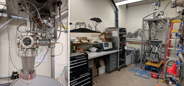
Figure 6.15: Final XeBrA assembly. Left: View of the xenon volume before the application of superinsulation with the purity monitor attached to the right of the central volume with viewports. The PMT is attached at the back. Right: Superinsulated hardware waiting to be enclosed in the OV. The edge of the gas system is visible on the right of the picture.

6.3.4 Outer vessel

The experimental chamber is wrapped in multiple layers of superinsulation and located inside an outer vacuum vessel (OV) for thermal insulation from the room as shown in Figure 6.15. Nevertheless, a small amount of heat $\mathcal{O}\left(10\,\mathrm{W}\right)$ still reaches the chamber, which causes xenon bubbles to be present in the apparatus. A 0.14 barg (2 psig) pressure relief valve prevents overpressure of the OV. An HV feedthrough identical to the ones used in the oil tank electronics is installed in an ISO100 port and connects the power supply to the apparatus.

The HV feedthrough in the vacuum space can cause an x-ray hazard if a breakdown occurs between the feedthrough and the OV. When this fault condition occurs, electrons generated during the discharge produce Bremsstrahlung photons while scattering off the aluminum of the OV. LBNL’s engineers modeled this effect using the MCNP software [392]. The model evaluates the amount of radiation emitted if a fault condition occurs over 100 hours per year. The result of the simulation is shown in Figure 6.16. To ensure workers’ safety, the assumptions going into the simulation were maximally pessimistic. Since both the current and voltage are limited by the power supply, and the power supply automatically ramps down to 0 V when it trips, a more realistic approximation for the fault condition might be $\mathcal{O}\left(10\,\mathrm{s}\right)$ per year, were a breakdown to occur.

The simulation in Figure 6.16 evaluates various combinations of shielding material. It shows that placing Pb on the outside of the Al OV is most effective at attenuating the radiation. This is because for the x-ray energies $E_{\gamma}$, the dominant reaction in the lead (Pb) is photoelectric absorption. The cross section of the photoelectric effect $\propto\mathrm{Z^{4}}/E_{\gamma}^{3.5}$ [393] so it is particularly strong in Pb ($Z=82$) compared to Al ($Z=13$) and very effective at lower x-ray energies. Placing the Al before the Pb softens the x-ray spectrum via Compton scattering. This softer x-ray spectrum is then more easily absorbed via photoelectric absorption in Pb.

Figure 6.16: Expected dose rate for 75 kV on the cathode evaluated at 30 cm outside of the OV for a focused electron beam with normal incidence on the inside wall. Various combinations of shielding material were considered. A combination of 1/4-in of aluminum (Al) and 1/32-in (0.8 mm) of lead (Pb) located on the outside of the OV was chosen based on its best attenuation property. The shielding limits the dose rate to $\sim 1\,\mathrm{mrem/hr}$, below the $5\,\mathrm{mrem/hr}$ threshold for posting a radiation area. Note that for x- and $\gamma$-rays $1\,\mathrm{rad}=1\,\mathrm{rem}$.

This led to a design and installation of a 1/32 in (0.8 mm) Pb shield on the outside of the OV. Additionally, because lead is a toxin, the shield was wrapped in a vinyl coating, giving XeBrA its unique zebra print shown in Figure 6.15.

6.3.5 Cooling

The apparatus was cooled by a pulse tube refrigerator manufactured by Cryomech with cold head model PT805 and compressor model CP950. A pulse tube refrigerator is commonly used in cryogenic applications as it is a type of cryocooler that does not contain any moving parts in the low-temperature part of the device, which results in high reliability and low mechanical vibrations. An overview of PTR operations can be found in [394]. The cold head has two stages: it delivers 40 W of cooling power at 80 K at its $1^{\mathrm{st}}$ stage, and even though the $2^{\mathrm{nd}}$ stage was not used, it can provide 1.5 W at 10 K, well below the desired XeBrA operating temperatures. The compressor is cooled using the building’s low conductivity water.

The PTR removes heat from the xenon to maintain a constant temperature inside the apparatus. This is done through a heat exchanger. The heat exchanger is made from SS brazed to a copper plate that makes a connection with the $1^{\mathrm{st}}$ stage of the PTR. The incoming room temperature gas enters the condenser where it is cooled by the outgoing gas on the inside surface and the PTR on the outside surface. That causes the xenon to liquefy and fall into the apparatus. The inner part of the heat exchanger is made from an electroformed bellows located inside an SS cylinder to prevent mixing of the two streams. The outgoing cold gas exits through the evaporator as illustrated in Figure 6.19.

A set of heaters (power resistors) connected to a programmable power supply were installed on the brazed copper part of the heat exchanger to enable temperature control. During data taking the heater was controlled through the Slow Control and enabled stable pressure in the apparatus. A simple see-saw control was used: when the pressure in the apparatus decreased below a given threshold, the heater turned on, and once a higher threshold was crossed, the heater turned off.

Throughout the operations, bubbles were continually formed at the bottom of the apparatus at the base of the HV feedthrough. That is the location of the highest heat load since it was not superinsulated for two reasons. One was to not disturb electric fields in the region and two, due to the proximity of boil-off heaters. Bubbles are undesirable since they are known to decrease breakdown voltage. In an attempt to reduce the formation of bubbles, two thermal links were designed from oxygen-free high-conductivity copper and installed in the apparatus. They deliver $\sim 1.5\,\mathrm{W}$ of cooling power each to two different locations in the apparatus. One is fastened to the bottom flange of the spherical square, and the other is attached to the bottom flange of the HV feedthrough. Each thermal link takes part of the cooling power away from the heat exchanger and instead delivers it to a specific location. That place is therefore cooled below the xenon boiling point. Unfortunately, even though the thermal links reduced bubble formation, they did not eliminate bubbles entirely.

6.4 Gas system

The gas system delivers gas to and from storage bottles to XeBrA and enables circulation of gas during operations for continuous removal of impurities. It serves other purposes such as injection of calibration sources or gas sample analysis. Since XeBrA’s gas system is designed to handle clean noble gases, it is made from all-metal parts where possible, with most parts made out of stainless steel. It can be controlled either manually or via the Slow Control (see Section 6.5.2.1).

The primary goals of XeBrA’s gas system were the ability to perform warm vacuum pumping, slow cooldown and gas condensation, gas circulation, and both regular and emergency recoveries. It was also designed to be user-friendly and easy to operate. The tubing diameter was determined by the required gas flow rate and from experiences using other xenon gas circulations systems (such as LUX, see Chapter 2, and PIXeY [192]). Due to a lack of data for gasses other than air, it is very hard to calculate flow for noble gases; what follows is an outline of a quick back-of-the-envelope flow calculation for xenon gas.

To find the pressure drop per unit length of tubing, Reynolds number $Re$ is calculated. Reynolds number is a dimensionless quantity used to predict whether flow will be laminar ($Re<2300$), intermittent, or turbulent ($Re>4000$):

$$Re=\frac{QD_{H}}{\nu A}.$$ (6.10)

Here $Q$ is the volumetric flow rate, $D_{H}$ is the hydraulic diameter, $\nu$ is the dynamic viscosity of the fluid, and $A$ is the pipe’s cross-sectional area. Next, the pressure drop $\Delta P$ due to friction per unit length $L$ for a given mean fluid velocity $\left\langle v\right\rangle$ can be calculated using the Darcy-Weisbach equation:

$$\frac{\Delta P}{L}=f_{D}\cdot\frac{\rho\left\langle v\right\rangle^{2}}{2D_{H}}$$ (6.11)

where $\rho$ is the density of the fluid and $f_{D}$ is the Darcy friction factor that can be looked up in a Moody chart [395]. This provides the pressure drop across some idealized parts, such as a piece of straight tubing. To find the pressure drop across a bent piece of tubing, a minor loss can be calculated using

$$\Delta P_{minor}=\xi\frac{\rho}{2}\left(\frac{Q}{A}\right)^{2}$$ (6.12)

where $\xi$ is the minor loss coefficient that is usually determined empirically. For a $90^{\circ}$ elbow $\xi=0.3$.

Additionally, some parts purchased from manufacturers quote a flow coefficient, which describes the relationship between the pressure drop and flow rate. Pressure drops for different gas system components at 20 standard liters per minute (SLPM) are shown in Table 6.2.

Tubing diameter [in]	Drop along straight tube [mbar/m]	Drop due to $90^{\circ}$ bent [mbar/m]
1/4	16.0	3.50
3/8	1.4	0.40
1/2	0.2	0.06

Part	Drop due to component [mbar]
LUX getter (from data)	700
Swagelok 1/4 in valve	10
Flow meter	30

Table 6.2: Top: Calculated pressure drops across tubing of varying diameter at 20 SLPM. Bottom: Pressure drop across varying gas system components.

Based on the above calculations and experience from other detectors the main gas system panel consists of 3/8-in diameter tubing. Most flexible hoses connected to the panel are 1/2-in diameter, except for the hose connecting the apparatus outlet to the pump inlet, which is 3/4-in. That is the region of lowest pressure in the system, and a larger diameter tubing causes smaller pressure drops (see Table 6.2). Additionally, purges are connected to the gas system using 1/4-in flexible hoses.

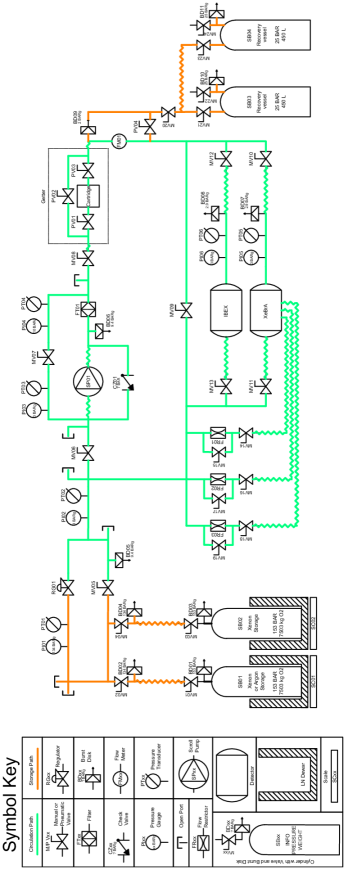
Figure 6.17: XeBrA’s P&ID.

The final XeBrA piping and instrumentation diagram (P&ID) is shown in Figure 6.17. Once the P&ID was complete, the design of the physical construction of the hardware began as outlined in Figure 6.18. First, a sketch of the physical location of the parts was created in AutoCAD. The individual components were welded using Swagelok’s orbital welder as needed. Then the gas system parts were pre-assembled on an aluminum panel to locate holes for attachment of valves and other components. Once the holes were drilled, the gas system was assembled and thoroughly helium leak checked. The final gas system panel was mounted on a seismically anchored 80-20 frame that also houses all of the other gas system components, such as the pump and the getter.

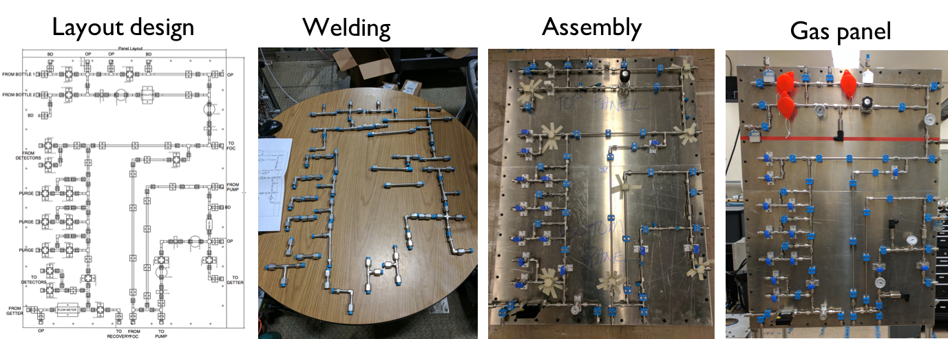
Figure 6.18: From left to right: First, the layout was optimized in AutoCAD. Then, various parts were welded as needed. The gas system was then assembled attached to an aluminum panel for support and leak checked.

6.4.1 Gas system extensibility

Even though XeBrA was the first to benefit from this easy-to-operate gas system, the gas system was designed to serve two experiments, XeBrA and IBEX, as can be seen from Figure 6.17. Only one apparatus can use the gas system at a time, but both can remain plumbed in. Therefore, once one experiment finishes taking data, the other one can start operating soon afterward (there is a short delay as the frozen recovered xenon must return to room temperature). There are a few particular components of the gas system worth highlighting.

The gas system uses an oil-free scroll pump for circulation made to order by Air Squared. A ceramic-based filter removes particles smaller than $0.003\,\mathrm{\mu m}$ from the flow downstream of the pump. Operating the pump in a vacuum can damage it, so a check valve is installed leading from the pump outlet to the pump inlet. If a pressure difference between the pump ends exceeds the threshold set on the check valve, the valve will open, thus equalizing the pressure and preventing pump damage.

Three purge lines were installed in XeBrA to prevent stagnation of xenon gas in parts not directly connected to the main circulation. If xenon is not circulated through the getter on a regular basis, outgassing of components can contaminate the gas. One purge line each leads out of the xenon gas space from the purity monitor arm and the PMT arm. The third purge line is connected to the xenon gas space near the linear shifter. Only a small gas flow is desired through the purges to ensure sufficient flow through the heat exchanger. This was achieved by installing flow restrictors inline as shown in Figure 6.17.

Figure 6.19 shows the connections of the plumbing lines inside the OV. The blue lines indicate the main flow. The incoming warm gas enters through the condenser. Most of the xenon that evaporates from the apparatus exits through the evaporator. A small fraction of gas exits through the purge lines (green). Additionally, there is a line that connects the purge lines to the gas inlet which ensures that the pressure of the gas entering the condenser matches the pressure in the gas above the main bath. This makes the liquid in the condenser fall into the main bath.

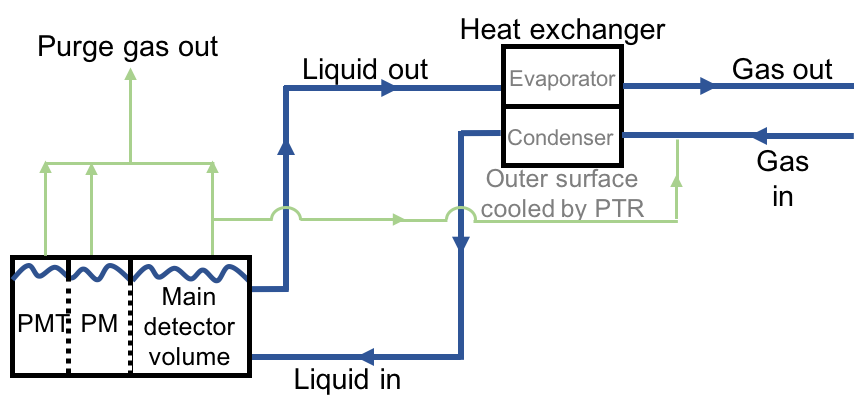
Figure 6.19: Schematics of the plumbing inside the vacuum space.

A brass parallel plate capacitor located directly above the ground electrode as shown in Figure 6.10 monitors the liquid level height during the condensation phase. The change in capacitance between the brass discs acts as a level sensor and determines when both electrodes are fully submerged in liquid. The relative dielectric constant of vacuum $\varepsilon_{r\,vacuum}=1$, while that of LXe $\varepsilon_{r\,LXe}=1.85$ and $\varepsilon_{r\,LAr}=1.5$. The expected change in capacitance in LXe is given by

$$\Delta C_{LXe} =\varepsilon_{0}\frac{A}{d}\left(\varepsilon_{r\,LXe}-\varepsilon_{r\,vacuum}\right)$$

$$=48\,\mathrm{pF}$$

where $A=48.33\,\mathrm{cm^{2}}$ is the area of the capacitor, $d=0.76\,\mathrm{mm}$ (0.03 in) is the separation of the two capacitor discs, and $\varepsilon_{0}=8.85\times 10^{-12}\,\mathrm{F/m}$ is the permittivity of vacuum. A similar calculation reveals a change in capacitance for argon $\Delta C_{LAr}=28\,\mathrm{pF}$. The wires connecting the level sensor to a capacitance meter contribute to the total capacitance of the system, which was measured to be $\sim 160$ pF in LXe. The change in capacitance between the brass discs was large enough to suffice for the operation of the level sensor.

6.4.2 Xenon recovery via cryopumping

At the end of regular operations, xenon is recovered via cryopumping. Cryopumping uses a cold surface to produce a vacuum in the enclosed space. In this particular case when xenon recovery is desired, a high-pressure aluminum storage cylinder located inside a stainless steel open top dewar is cooled with liquid nitrogen (LN), and xenon from the apparatus is allowed to flow into this cylinder as shown in Figure 6.20. There, the xenon freezes to the inner walls of the cooled cylinder since the boiling temperature of LN is 77 K while the melting point of xenon is 161 K. It is important to keep the pressure in the apparatus above the xenon triple point throughout this operation to prevent xenon freezing inside the apparatus. To speed the recovery, two 100 W heaters are installed at the bottom of the apparatus to encourage xenon boiling. Additionally, heat should be provided to the top portion of the aluminum cylinder, including the valve, to prevent it from freezing. Because both the valve and the seal between the valve and the cylinder contain elastomer seals, extreme temperatures (both hot and cold) might damage those and allow xenon to leak into the room.

Once all the xenon has left the apparatus and is recovered into the cylinder, the valve on the top of the cylinder is closed, and the cylinder is allowed to warm. The xenon is contained within the aluminum storage cylinder until its next use. To recover the entire amount of xenon contained in XeBrA takes about one full working day. Further details and particular steps of this procedure are included in Appendix C.

At the end of operations with liquid argon, argon is slowly released into the room since argon is not very expensive.

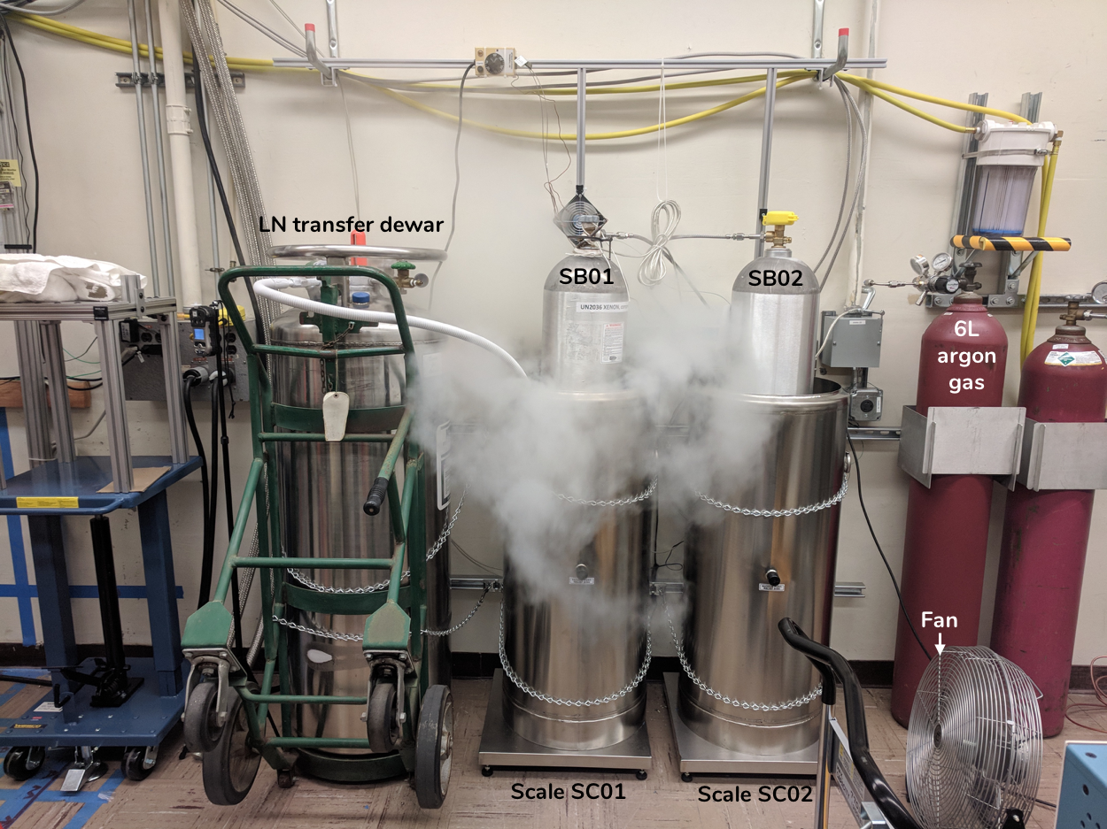
Figure 6.20: Xenon recovery via cryopumping in progress. Xenon is being recovered from the apparatus into SB01.

6.4.3 Xenon emergency recovery

The standard recovery via cryopumping requires LN and needs to be planned. If the xenon cannot be recovered using the standard recovery procedure, a safety burst disc (BD07 in Figure 6.17) would rupture and vent xenon into the room once the pressure in the apparatus rises above 3.9 bar. Such a situation might arise if a hardware or a power failure occurs. A power failure halts apparatus cooling, and the increased heat load results in a rise of pressure inside the apparatus within $\sim 1$ hour. The room ventilation is also interrupted during a power failure. The lack of air circulation in the room would prevent xenon recovery via cryopumping as it would pose an ODH hazard. A low-pressure passive recovery system was implemented to avoid this xenon loss.

Two large (450 l) tanks are plumbed in parallel and act as a single 900 l volume, as shown in Figure 6.21. Affectionately known as Hippo and Rhino, these two tanks can store the entire quantity of xenon contained in XeBrA during operations at room temperature at low pressure. The 900 l volume of the recovery tanks is large enough to hold $\sim 16\,\mathrm{kg}$ of xenon after it has boiled and warmed to room temperature at a pressure of 3.3 bar. This is below the 4 bar absolute pressure at which the BD07 burst disk would otherwise vent the xenon into the 70A-2263 lab.

The combined volume is evacuated before operations and plumbed into the gas handling system as shown in Figure 6.17. In normal operation, a 3 barg burst disk (BD09) separates the apparatus from the recovery tanks. If the pressure inside the apparatus at any time exceeds 2 barg, BD09 will open, connecting it to the 900 l evacuated volume of the low-pressure recovery tanks. However, a burst disc rupture is irreversible, so a pneumatic valve (PV04) is installed in parallel with the burst disc. The valve opens automatically if a high-pressure alarm threshold in the Slow Control is exceeded. For this to be effective, the alarm threshold must be below 2 barg and is typically set to 1.8 barg. The valve also automatically closes once the pressure drops below the alarmed threshold.

Once the emergency is over, xenon from Hippo and Rhino can be cryopumped back to the storage bottles SB01 and SB02.

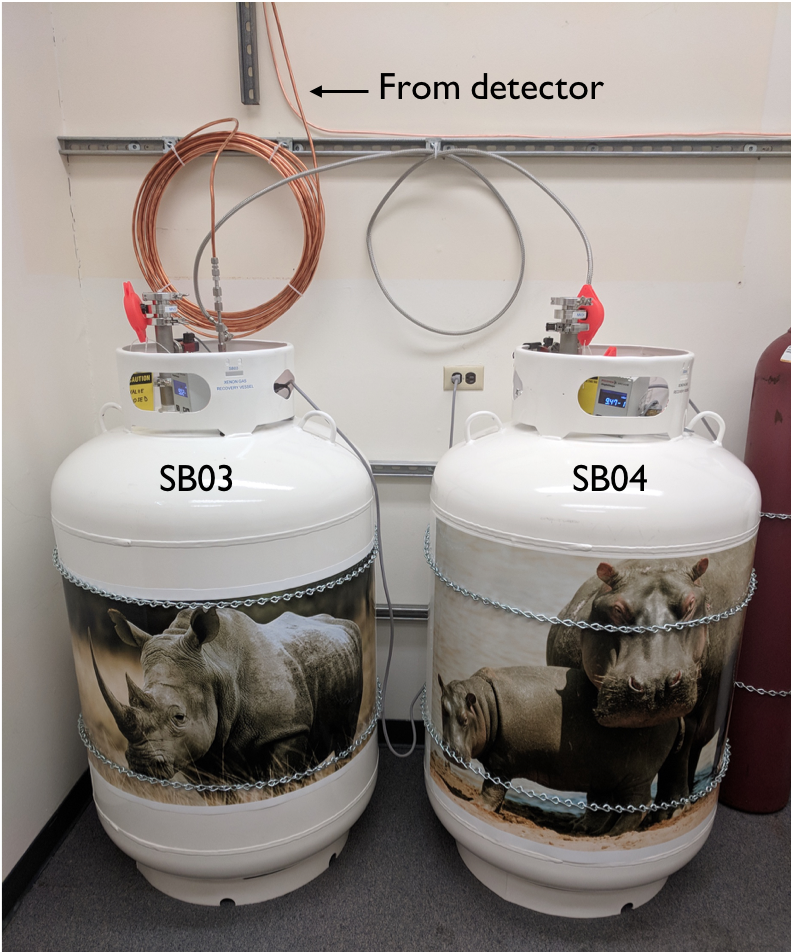
Figure 6.21: Passive xenon recovery system, known as Hippo (SB04) and Rhino (SB03). The tanks are connected through a flexible hose and to XeBrA via 100 ft of 5/8-in clean copper tubing. Each tank has a vacuum gauge for pressure monitoring and is chained to the wall for seismic safety (to prevent wildlife escape).

6.5 Operations

The core components of XeBrA are the apparatus and the gas system. There are multiple other supporting components required for successful operation. Since the apparatus and the sub-components take up physical space, their intelligent placement within the lab can affect operations. Detailed procedures were developed to ensure safe apparatus operation without loss of valuable xenon. Several electrical components were installed for apparatus stability monitoring, and a software system was implemented to enable data collection and 24/7 and remote operations.

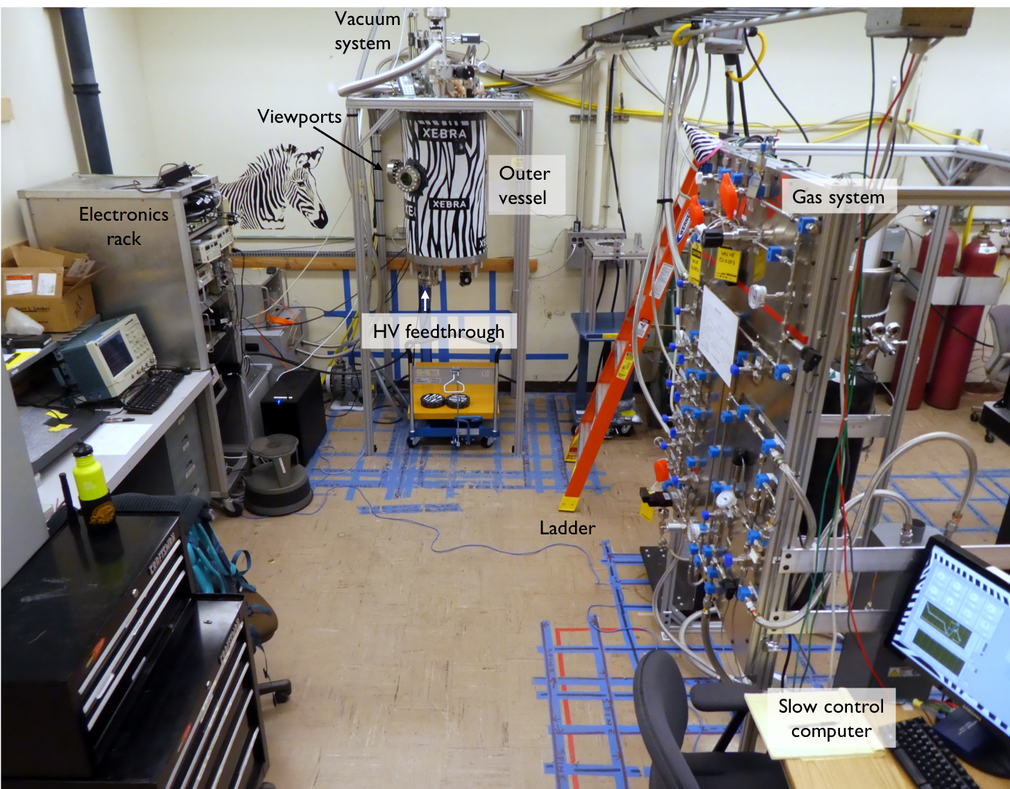
Figure 6.22: Overview of the lab.

The limited floor space at LBNL in lab 70A-2263 where XeBrA is located required careful optimization of equipment placement, ultimately resulting in the floor plan illustrated in Figure 6.23. A picture of the final layout of the lab is shown in Figure 6.22. This final layout achieves two real-world practical goals: both XeBrA and IBEX fit in the space available, and an individual attempting to operate XeBrA has all of the controls and monitors available to herself within a few steps. And of course, there are clear paths for emergency escape.

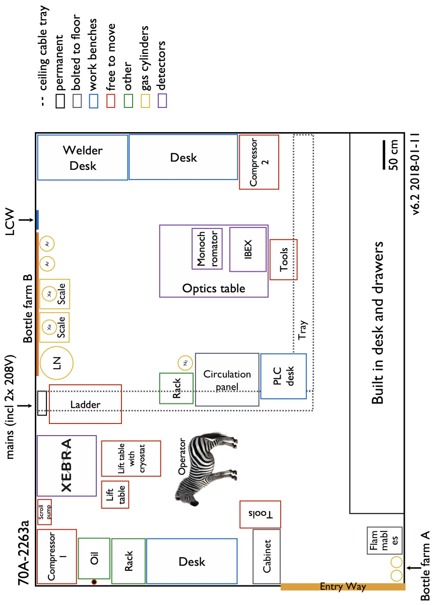
Figure 6.23: The layout of the lab space in 70A-2263 at LBNL.

An integral part of working at a national lab is a long list of training required to do anything from purchasing apparatus parts, standing on ladders, to cryogen handling. During my time at the lab, this has resulted in forty various training courses listed in Figure 6.24. This does not include many, many more courses passed for on-site LUX shifts at SURF and safety training at UCB.

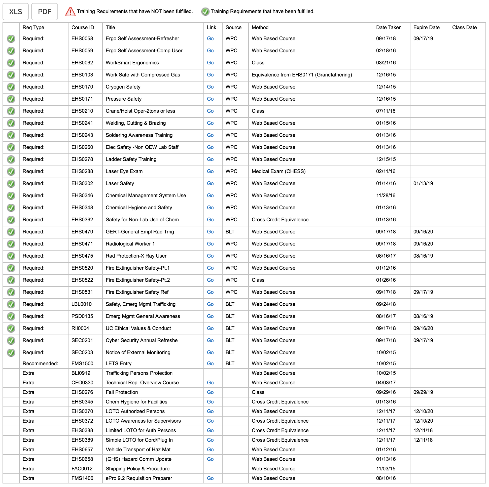
Figure 6.24: List of training courses passed while at LBNL.

6.5.1 Procedures

Procedures for operating the gas system and the apparatus were developed for use in cases with both LAr and LXe. Appendix C contains the procedure for xenon condensing, circulation, and recovery in XeBrA.

6.5.2 Performance monitoring

To monitor parameters during operations and data taking, the following components were installed in the apparatus. All of them were monitored in the Slow Control described in the next section.

• Resistance temperature detectors (RTDs): RTDs consist of a wire of pure platinum housed in a protective probe. The material has an accurate resistance vs. temperature relationship, which is used to indicate temperature. There are 8 RTDs installed throughout the apparatus to monitor temperatures of the various parts.

• Pressure gauges and pressure transducers: Pressure gauges have physical dials while pressure transducers are read out in the Slow Control. They serve to monitor pressure throughout the apparatus as indicated on the P&ID (Figure 6.17). An additional pressure transducer is located on the nitrogen gas bottle that supplies gas needed for pneumatic valve operation.

• Xenon scales: Each of the two storage bottles is located on a scale which enables direct measurement of the amount of xenon that has entered the apparatus.

• Vacuum gauges: Several vacuum gauges monitor pressure inside the OV and the recovery vessels.

• Picoammeter & charge amplifier: These were connected to the ground electrode (anode) and provided monitoring of current during data taking. The charge amplifier was read out by a DAQ system rather than the Slow Control.

6.5.2.1 Slow Control

Figure 6.25: Slow control screenshots. a: Overview of the gas system. b: Overview of the HV stand with controls for HV data taking. c: Pressure monitoring. d: Interlock screen.

Maintaining stability in XeBrA’s day-to-day operations requires manipulation of a few critical components. The pressure, temperature, and gas circulation speed all increase and decrease depending on the settings of the heaters, pump, and other regulators in the system. Slow control is a well-tested solution for monitoring of gas flow and apparatus status, automation of controls, and remote operations at time scales ranging from 0.1 seconds to weeks. Low and high alarms can be set on various parameters. If a set of conditions is met, interlocks trigger automatic shut-off of selected parts of the system (getter, pump) or ultimately start xenon emergency recovery. A user can be informed about any alarms through an email system which can be forwarded to a mobile phone to sound noisy alarms at any time. This mitigates risks resulting from apparatus operations that span multiple day-night cycles. Additionally, the Slow Control also provides two data logging modes: a slow mode that can log apparatus stability every few seconds, and a fast mode with an ability to save data every 100 ms used for HV breakdown data collection. Several screenshots from XeBrA’s slow control are included in Figure 6.25.

The Slow Control backend runs on programmable logic controllers (PLCs), flexible, easily programmable digital computers known for their high-reliability automation. The frontend runs on LabView [396], a visual programming language often used for data acquisition, instrument control, and automation. XeBrA’s Slow Control was developed by Mark Regis, an engineer at LBNL.

6.6 Data collection

Data collection started in February 2018 and continued until September 2018. During that time, XeBrA was filled twice with argon, and twice with xenon, resulting in four different data acquisitions described in this section and summarized in Table 6.3.

	Liquid	Electrode separation	Pressure	Purity	Purity
		[mm]	[bar]	[$\mu$s]	[ppb]
Run 0	Ar	1-8	N/A	223	2
Run 1	Ar	1-6	1.5, 2	400	1
Run 2	Xe	1-5	2	N/A	>ppm
Run 3	Xe	1-2	2	2.2	200

Table 6.3: Summary of data acquisitions. Only Runs 1, 2, and 3 were used in analyses since pressure during data acquisition varied in Run 0. The temperature of the liquid is not known due to the poor thermal coupling of RTDs. Additionally, there was a temperature gradient present in LXe and LAr during data acquisitions.

6.6.1 Run 0 (liquid argon)

Data collection in XeBrA started in early 2018. Careful planning occasionally pays off, and all the components worked as expected during the first cool down with LAr in February 2018 (Run 0). However, it was discovered that LAr was forming gas bubbles near the bottom of the HV feedthrough cone. These bubbles rose through the apparatus, flowed through the active volume, and distorted breakdown datasets. To avoid bubbles during data acquisition, the apparatus was kept at low pressures overnight ($\sim 1.3\,\mathrm{bar}$). Then, during the data acquisition, the pressure was slowly increased in the apparatus by increasing the heat load on the heat exchanger. This enabled several hours of bubble-free data taking, but at varying pressure.

Data were acquired at 1, 5, 7, and 8 mm electrode separations between February 17-19, 2018. Figure 6.27 shows a photograph of a spark during data acquisition in LAr in Run 0. The purity of LAr was $\sim 223\,\mathrm{\mu s}$ as measured by the purity monitor described in Section 6.3.2. This corresponds to $\sim 1\,\mathrm{ppb}$ oxygen equivalent impurities. The conversion from $\mu s$ to ppb was described in Section 5.3.4.2. Because of the varying pressure, the data were not included in any analyses discussed in this work.

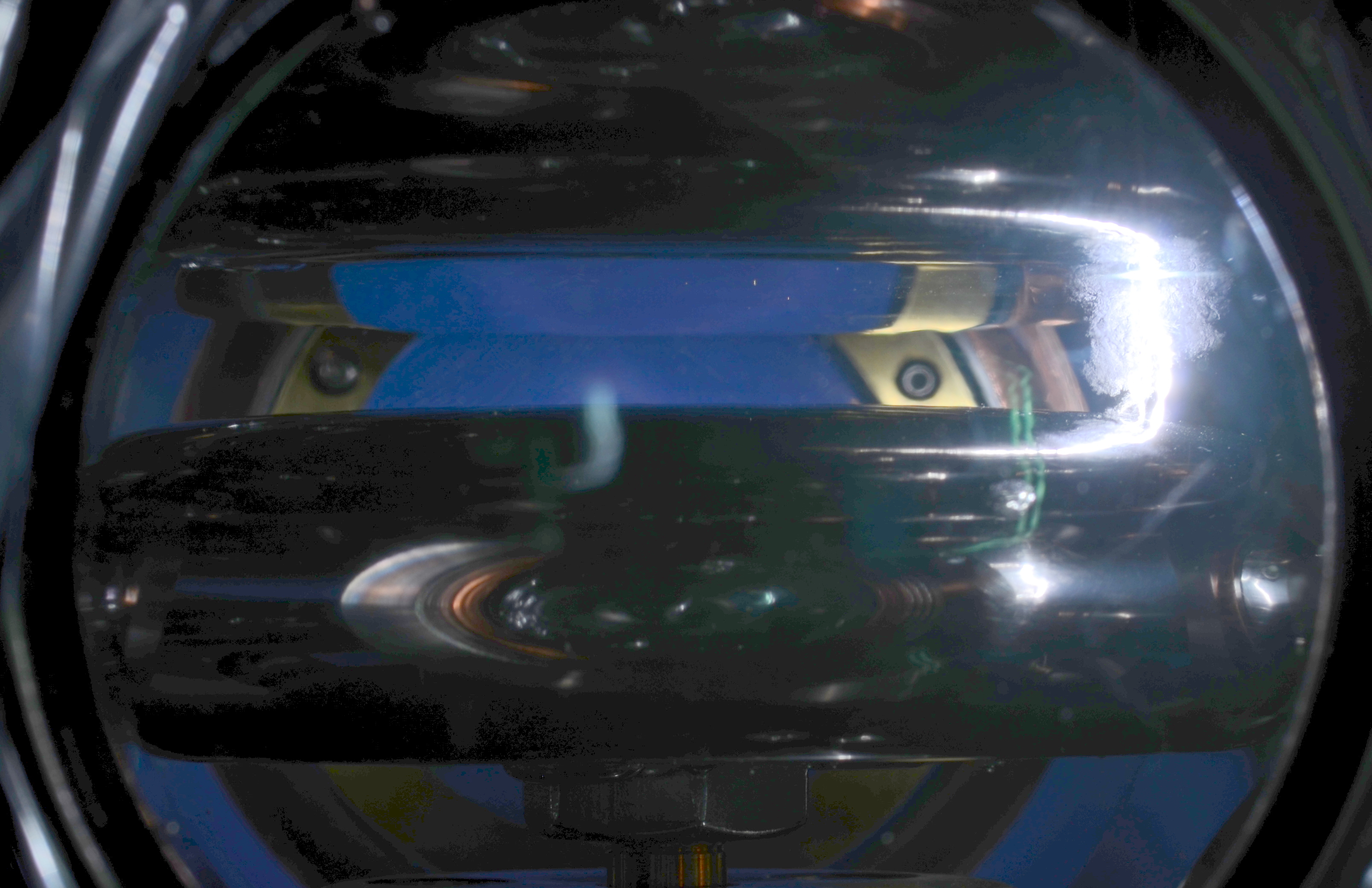
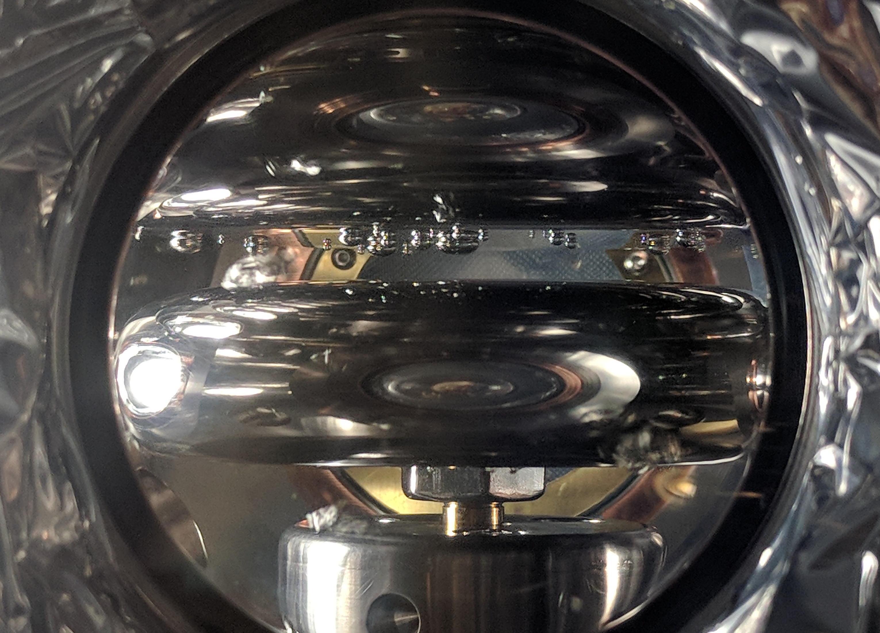
Figure 6.26: Photograph of a spark near the edge of the electrodes during data acquisition in LAr in Run 0. Photograph by Ethan Bernard.

Figure 6.27: Photograph of bubbles in the LAr active volume between data acquisitions in Run 1. A couple forming bubbles are visible at the top of the alignment joint and behind the electrodes.

6.6.2 Run 1 (liquid argon)

In an attempt to reduce the number of bubbles in the apparatus a thermal link, described in Section 6.3.5, was introduced to XeBrA for the next data acquisition in LAr (Run 1). This improved the bubble situation, but not entirely: bubbles that were visible in the apparatus are shown in Figure 6.27. There is evidence in the literature that pressure affects breakdown [350, 292], so unlike in Run 0, a procedure was developed to achieve data acquisition at a stable pressure. The apparatus was kept at lower pressures overnight. Then, throughout the data acquisition, argon from a storage bottle was slowly added. This caused a brief pressure increase at the beginning after which the pressure remained constant for a couple of hours while the additional argon was condensing and the apparatus was free from bubbles.

Therefore, data were collected at two different pressures, 1.5 and 2.0 bar. Usually, data taken at 1.5 bar were obtained first in the morning, while data at 2 bar were collected in the afternoon since a pressure increase temporarily suppressed bubble formation. Figure 6.28 illustrates the behavior of pressure and temperature throughout one of the periods of data acquisition. LAr data used in analyses were collected between May 26 and June 8, 2018. The purity of LAr was $\sim 400\,\mathrm{\mu s}$, which corresponds to $\sim 1\,\mathrm{ppb}$ oxygen equivalent impurities.

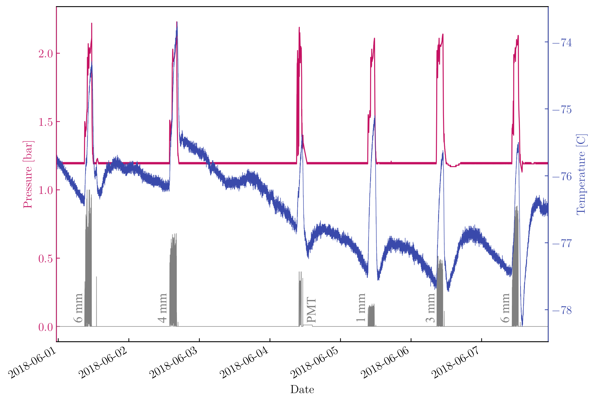
Figure 6.28: Pressure and temperature during operations in LAr. Pressure, as measured by PT05, is shown in pink. Due to the poor thermal coupling of RTDs, the absolute temperature in the apparatus is not known, but changes in temperature as measured at the bottom of the HV cone are shown in blue. For illustration, the gray line shows the normalized voltage of the power supply to indicate the period of data taking at various electrode separations.

6.6.3 Run 2 (liquid xenon)

After the successful data acquisition in LAr, the apparatus proceeded to LXe operation (Run 2) in July 2018. Only the PMT was changed between data acquisitions in LAr and LXe, everything else remained intact. There were significantly fewer bubbles present in the apparatus when operated in LXe. Unfortunately, even a small amount of bubbles is disruptive to HV breakdown measurements, so the same pressure trick employed in LAr in Run 1 was used to collect LXe data. The data taking procedure is detailed in Section C.6 of the xenon procedure included in Appendix C.

Data were acquired on July 12, 2018, at 2 bar. The behavior of the detector is shown in Figure 6.29. Since the purity monitor did not work in liquid xenon, a residual gas analyzer (RGA), a small quadrupole mass spectrometer, was used to estimate the amounts of impurities in LXe during Run 2. Based on that measurement, we estimate that the LXe purity had $>\mathcal{O}\left(\mathrm{ppm}\right)$ oxygen equivalent impurities during Run 2. It was later discovered that the xenon used was polluted by air during cylinder filling at Yale.

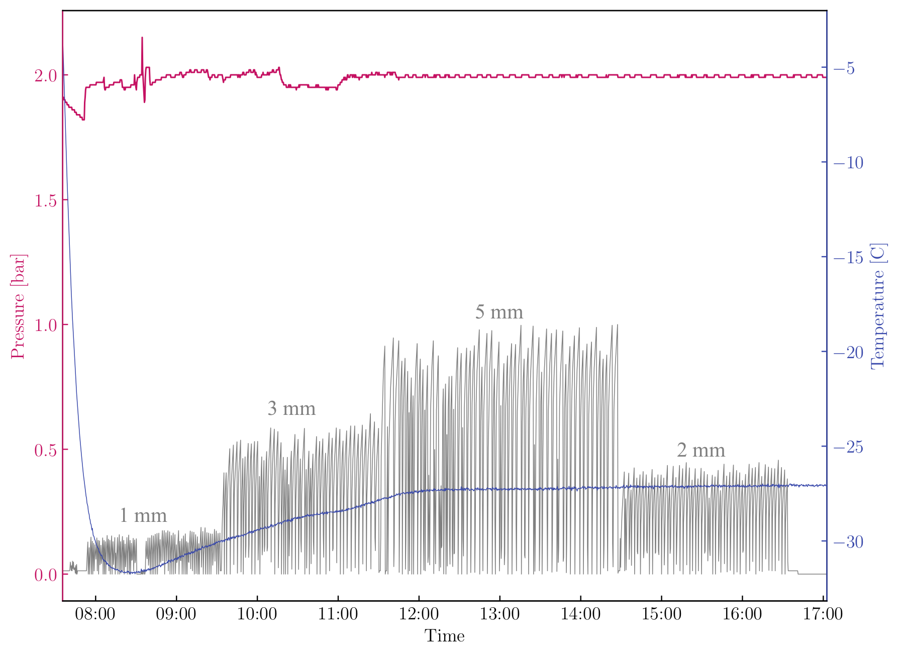
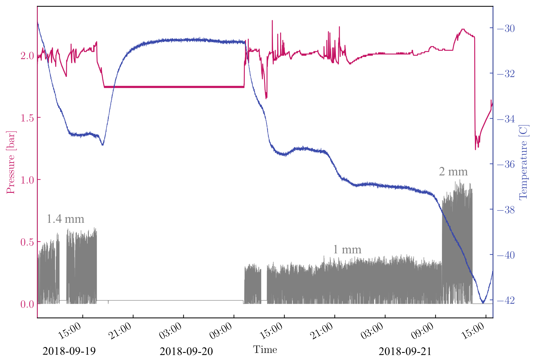
Figure 6.29: Pressure and temperature in the apparatus during operations in LXe. Pressure, as measured by PT05, is shown in pink. Due to the poor thermal coupling of RTDs, the absolute temperature in the apparatus is not known, but changes in temperature as measured at the bottom of the HV cone are shown in blue. For illustration, the gray line shows the normalized voltage of the power supply to indicate the period of data taking at various electrode separations. Top: Run 2. Bottom: Run 3. There is a noticeable drop in pressure between HV data at 1.4 and 1 mm, which shows the preparation period for the 1 mm data acquisition.

6.6.4 Run 3 (liquid xenon)

A new getter cartridge and two chemical inline purifiers were installed prior to the second xenon data acquisition (Run 3) in September 2018. The apparatus was filled with clean xenon from the LUX detector. Additionally, the location of one of the thermal links was moved to the bottom of the HV cone in an attempt to further minimize bubbles. The xenon procedure included in Appendix C was used for data collection as in Run 2. However, this time the xenon was added through a series of inline purifiers which have a high resistivity. This caused the circulation speeds to be much lower than in previous runs. That ultimately led to the formation of solid xenon in the apparatus. A small amount of solid xenon near the bottom of the HV feedthrough where all the bubbles were formed would be desirable as it would suppress the bubble formation in the apparatus, but frozen xenon also likely formed in the heat exchanger, which hindered its performance.

During an attempt to slowly warm up these parts of the apparatus, a weak weld of the heat exchanger burst open, which stopped XeBrA operations on September 23, 2018. Figure 6.30 shows frozen xenon that formed in the apparatus during the emergency xenon recovery. Consultation with Joe Saba, an LBNL engineer, suggested that the operational parameters of the heat exchanger were incorrectly specified before manufacturing, which eventually led to a rupture of a weld due to material fatigue. Plans to fix XeBrA to prepare it for future data acquisitions are underway.

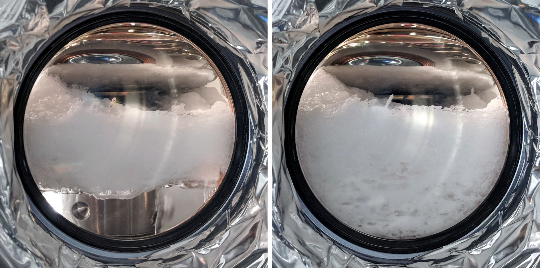
Figure 6.30: Left: Layer of frozen xenon being formed on top of liquid xenon. Right: Xenon slushee.

Some data were collected before the detector stopped working, on September 19-21, 2018. All data were obtained at 2 bar absolute pressure. In an attempt to obtain a larger sample size to study the spread of the data, many breakdown voltages were recorded for one fixed electrode separation. Figure 6.29 illustrates the behavior of pressure and temperature throughout data acquisitions.

To estimate purity of LXe during Run 3, XeBrA was temporarily transformed into a small TPC during the initial LXe condensation. The two electrodes were separated by 20 mm, the maximum possible distance allowed by hardware design. The fill was stopped once the liquid level was 5 mm below the top electrode. The electrodes could then be biased to create drift and electroluminescence regions between them. Due to EH&S regulations, we were unable to use radioactive sources with short notice, so instead naturally occurring radioactivity from old thoriated welding rods was used. Several such rods were attached to the outside of the OV, and the PMT was used to record the data overnight. A fit to the plot of $\log_{10}(\mathrm{S2/10)}$ vs. drift time revealed an electron lifetime of $\mathrm{2.2\,\mathrm{\mu s}}$. Using Equation 5.17, this corresponds to $\sim 200$ ppb oxygen equivalent impurities.

6.6.5 Review of apparatus parameters

This section serves as an overview of parameters that pertain to data collection.

The voltage delivered by the Spellman power supply was monitored by the Slow Control every 100 ms, along with pressure measurements (PT05) and readings from the picoammeter. Additionally, the signal from a charge amplifier connected to the ground electrode was recorded by the DAQ computer. HV breakdown was defined as the voltage where the current drawn by the power supply exceeded the $10\,\mathrm{\mu s}$ current limit imposed on the power supply. After a current trip, the power supply automatically ramps down to 0 V. During data acquisition, HV was slowly ramped up using an automated system in Slow Control. This allowed three different ramping speeds as shown in Figure 6.25.b. Table 6.4 includes the value of the ramp parameters used during data acquisitions along with other parameters relevant to the analysis.

Parameter	Value	Unit
Electrode material	303 SS
Cathode surface finish (Ra)	$0.05$	$\mu$m
Anode surface finish (Ra)	$0.07$	$\mu$m
Power supply limit	-75	kV
Trip current	10	$\mu$s
Cable capacitance	203	pF
Ramp speed 1	30-60	kV/min
Ramp speed 2	12	kV/min
Ramp speed 3	6	kV/min
Wait period	10-20	s

Table 6.4: Summary of apparatus parameters that pertain to data collection. Cable capacitance refers to the length of the cable between the oil box and the apparatus.

The electrode separation was found by zeroing the caliper on the linear shifter as the electrodes touched faces. At each separation, dozens to hundreds of breakdown events were measured. This analysis uses the 90% stressed electrode area as estimated using COMSOL Multiphysics simulations of the system. The values of 90% stressed area and volume at different electrode separations are summarized in Table 6.5.

To achieve a comparable state for measurements at each electrode separation, usually, data at a given separation were collected during one day after the apparatus was held stable overnight. This resulted in more data points taken at smaller separations since it takes less time to ramp up to lower voltages. The location of the spark on the electrode appeared to vary. Since the detector was not assembled in a clean room, a small amount of debris or speckles of dust were visible on the electrode surfaces, usually near the beginning of each run. The debris moved away from the electrode surfaces due to liquid circulation, effects of breakdown, and bubbles.

Separation	Radius	Area	Volume	$\mathrm{C_{LXe}}$	$\mathrm{C_{LAr}}$
[mm]	[mm]	$\left[\mathrm{cm^{2}}\right]$	$\left[\mathrm{cm^{3}}\right]$	[pF]	[pF]
1.0	18.9	11.22	1.12	18.4	14.9
1.4	21.0	13.85	1.94	16.2	13.1
2.0	23.3	17.06	3.41	14.0	11.3
3.0	26.0	21.24	6.37	11.6	9.4
4.0	28.2	24.98	9.99	10.2	9.3
5.0	30.2	28.65	14.33	9.4	7.6
6.0	32.2	32.57	19.54	8.9	7.2
7.0	34.2	36.75	27.73	8.6	7.0

Table 6.5: Values of 90% stressed electrode area and volume as simulated by COMSOL Multiphysics. Also tabulated is the capacitance caused by LAr and LXe between the electrodes at various separations.

6.7 Sparks

Before we examine the data in aggregate, it is interesting to investigate the behavior of individual sparks visually. Several videos of sparks at different electrode separations were recorded in LAr and LXe with a point-and-shoot camera and a cell phone. Despite the slow frame rate of these devices, some videos reveal information about spark development.

6.7.1 Liquid argon

Breakdown behavior of sparks in LAr has been studied in detail previously and was published in [314]. The spark registered in XeBrA shown in Figure 6.31, appears to have very similar behavior. The work of [314] can be used to explain its evolution.

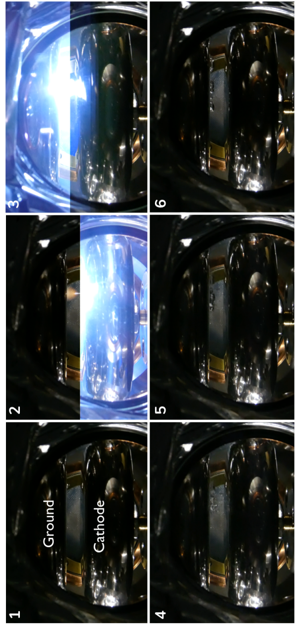
Figure 6.31: Spark development in LAr at 7 mm electrode separation. Frame 2 captures the initial light cone, the subsequent filament, and the final emission of light. The individual images were not taken at regular intervals. The sequence was captured by Panasonic Lumix DMC-ZS60 camera.

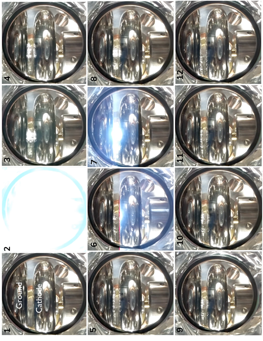
Figure 6.32: Step-by-step development of breakdown in LXe at 5 mm electrode separation with HV electrode (cathode) at $\sim-53\,\mathrm{kV}$. Two sparks arise from the breakdown. The first, larger spark (frames 1-5) creates bubbles that in turn likely cause the second spark (frames 6-12). The duration of the entire event is $\sim 0.9\,\mathrm{s}$. The second spark happens 0.6 s after the first spark. After the spark is over, the bubbles slowly leave the area. Screenshots were taken from a video recorded by a Pixel XL phone at 60 fps at irregular intervals. The red line in frame 6 is an artifact from the phone recording rather than a result of the spark.

Frame 2 shows the field emission of electrons that ionize and excite argon atoms on their way to the anode. This creates the visible light cone, whose brightness increases from the cathode toward the anode. Positive ions are produced during this process. Once the positive ions reach the cathode surface, they raise the local temperature, and the liquid near the initial discharge point forms a bubble. This leads to a formation of plasma with an increased conductivity resulting in a decrease of the electric field near the initial field emission point. This suppresses further growth of the initial field emission current, while the electrons of the gas plasma force the bubble to elongate and grow. The streamer then collapses to its well-known filament shape. As the streamer propagates toward the anode, it is subject to thermodynamic fluctuations at its forefront at the liquid-gas boundary, which results in the random path of the filament.

When the streamer reaches the anode a short light emission is registered (frames 2-3). The exact mechanism for this light emission is unknown, but it might be triggered once the filament loses its thermodynamic stability and expands into a gas bubble, where an arc discharge forms. This is accompanied by an acoustic shock and an extensive production of gas bubbles on the anode near the location of the discharge (frames 4-6).

For further details about the development of the spark, along with a spectral analysis of the light emitted throughout the process and a well-documented time evolution of each step, consult Reference [314].

6.7.2 Liquid xenon

Figure 6.32 shows the evolution of a spark in LXe. The spark is created on the cathode and propagates up to the grounded anode. A second spark follows shortly, likely caused by bubbles of the first spark.

6.8 Results

We now proceed to the analysis of the data. There are multiple sources of data that might contain interesting information. Here, we focus only on HV data from the power supply recorded by the Slow Control. A more detailed analysis that includes data from the picoammeter, the charge amplifier, and the PMT will follow in the future.

First, the expected errors of the measurements are discussed in Section 6.8.1. Results from LAr are presented in Section 6.8.2 and results from LXe are presented in Section 6.8.3. Due to XeBrA’s unique construction, data from LAr and LXe can be compared directly. This was done in Section 6.8.5. Finally, a fit to Weibull function as predicted by the weak link theory is attempted in Section 6.8.6.

6.8.1 Statistical and systematic errors

The statistical error was low at each separation so systematic errors dominate the results presented in this work. The statistical error was calculated as the standard deviation of the mean breakdown value divided by the square root of the number of breakdowns at each electrode separation. Several sources of systematic error were considered. A 0.1 mm uncertainty was estimated for the electrode separation based on the mechanical error of zeroing the electrodes. Additionally, the effect of the tilt of the electrodes was considered. Based on a perception study, a 0.3^∘ tilt of the electrodes should be visible to a user. Since there are two uncorrelated axes along which the electrodes might be tilted (and two perpendicular viewports), this results in the 0.4^∘ systematic error. The effect of this tilt on the electric field was derived in Table 6.1 and is summarized in Table 6.6. A follow-up study could use two high-resolution photographs through XeBrA viewports to place more precise bounds on the alignment error. A 100 V uncertainty on the breakdown voltage was estimated based on the minimum power supply voltage increment.

Errors from pressure fluctuations and conditioning effects were also taken into account. To estimate the systematic error caused by the variation of pressure, the data were divided into low- and high-pressure subsets for each electrode separation. The difference in the average breakdown value for the lower and higher pressure datasets was then taken as a systematic error on the breakdown voltage. Similarly, to account for conditioning effects, the data at each electrode separation was split into two groups based on the time of data collection. The difference in breakdown voltage for the earlier and later halves of data was treated as a systematic error. All the systematic errors were treated as uncorrected uncertainties in the analysis. For the illustration of the size of each systematic error and the statistical error in LAr, the contributions are shown in Table 6.6.

The values of both statistical and systematic errors along with the combined error for LAr and LXe measurements are documented in Tables 6.9, 6.9, and 6.9.

$d$	$\Delta$ separation	$\Delta$ tilt	$\Delta$ voltage	$\Delta$ pressure	$\Delta$ conditioning	Statistical error	Combined error
[mm]	%	%	%	%	%	%	%
1	10	5	0.9	3.8	2.1	1.2	12.1
2	5	3	0.5	4.4	2.6	2.0	8.0
3	3	2	0.3	4.5	3.1	1.5	6.9
4	3	1	0.2	2.1	4.8	1.9	6.2
5	2	1	0.2	2.1	4.3	2.9	6.0
6	2	1	0.2	16.7	14.8	2.2	22.5

Table 6.6: Summary of systematic and statistical errors in liquid argon measurements. All errors are quoted as a percent error on the breakdown field.

6.8.2 Liquid argon data analysis

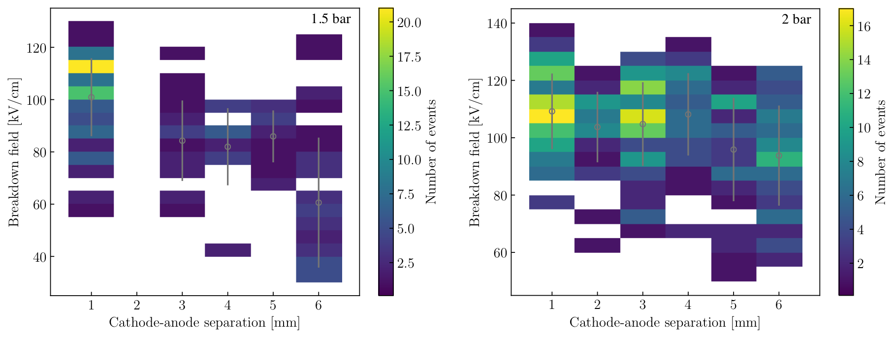
Figure 6.33: Histogram of breakdowns in LAr as a function of electrode separation. Data were taken at 1.5 bar (left) and 2 bar (right). The vertical bars indicate the standard deviation at each separation.

Figure 6.33 shows a histogram of breakdown events recorded in XeBrA for varying electrode separation at 1.5 and 2 bar. Tables 6.9 and 6.9 summarize the information about data acquired in LAr.

$d$	#	V	E	Statistical error	Systematic error	Combined error	P	$\sigma_{\mathrm{P}}$
[mm]		[kV]	[kV/cm]	[kV]	[kV]	[kV]	[bar]	[bar]
1.0	85	10.1	100.9	1.6	11.4	11.5	1.5	0.03
3.0	18	25.3	84.3	3.6	34.7	34.9	1.5	0.04
4.0	18	32.8	82.0	3.5	13.1	13.5	1.5	0.08
5.0	14	43.0	85.9	2.7	12.7	13.0	1.5	0.07
6.0	38	36.4	60.6	4.0	13.5	14.1	1.5	0.06

Table 6.7: Summary of breakdown data collected in XeBrA in LAr at 1.5 bar. Each data point is the mean value of all measurements from one run taken at the same gap distance. The electrode separation is referred to as $d$, # is the number of data points recorded at each separation, and $\sigma_{\mathrm{P}}$ is the standard deviation of the pressure.

$d$	#	V	E	Statistical error	Systematic error	Combined error	P	$\sigma_{\mathrm{P}}$
[mm]		[kV]	[kV/cm]	[kV]	[kV]	[kV]	[bar]	[bar]
1.0	104	10.9	109.2	1.3	13.1	13.2	2.0	0.05
2.0	35	20.7	103.7	2.1	8.1	8.3	2.0	0.06
3.0	91	31.4	104.8	1.5	7.0	7.2	2.0	0.07
4.0	47	43.3	108.2	2.1	6.4	6.7	2.0	0.06
5.0	41	47.9	95.9	2.8	5.0	5.8	2.0	0.06
6.0	73	56.3	93.8	2.0	21.0	21.1	2.0	0.07

Table 6.8: Summary of breakdown data collected in XeBrA in LAr at 2 bar. Each data point is the mean value of all measurements from one run taken at the same gap distance. The electrode separation is referred to as $d$, # is the number of data points recorded at each separation, and $\sigma_{\mathrm{P}}$ is the standard deviation of the pressure.

$d$ [mm]	#	V	E	Statistical error	Systematic error	Combined error	P	$\sigma_{\mathrm{P}}$
Run 2		[kV]	[kV/cm]	[kV]	[kV]	[kV]	[bar]	[bar]
1.0	75	10.0	99.5	1.1	20.1	20.1	2.0	0.02
2.0	55	25.5	127.5	1.2	8.3	8.3	2.0	0.00
3.0	51	32.6	108.7	1.7	13.5	13.7	2.0	0.02
5.0	68	52.5	104.9	1.7	14.0	14.1	2.0	0.00
Run 3
1.0	1215	9.6	95.9	0.4	18.7	18.7	2.0	0.03
1.4	234	15.2	108.3	1.1	25.5	25.5	2.0	0.03
2.0	108	26.4	131.8	1.3	16.3	16.4	2.0	0.03

Table 6.9: Summary of breakdown data collected in XeBrA in LXe at 2 bar. Each data point is the mean value of all measurements from one run taken at the same gap distance. The electrode separation is referred to as $d$, # is the number of data points recorded at each separation, and $\sigma_{\mathrm{P}}$ is the standard deviation of the pressure.

The characteristic behaviors of dielectric breakdown as a function of separation, stressed electrode area, and stressed volume are shown in Figures 6.35, 6.35, and 6.37, respectively. Figure 6.35 combines experimental data available in the literature with data obtained in XeBrA at 1.5 bar.

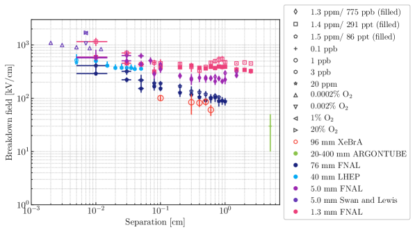
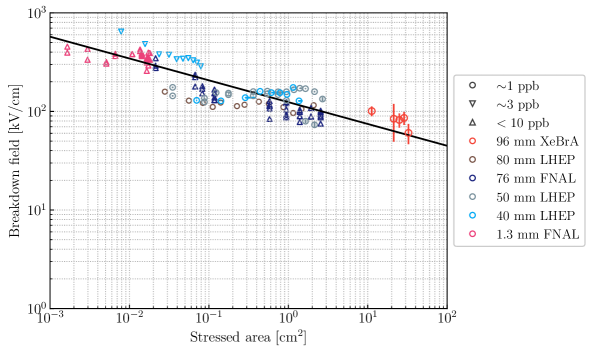
Figure 6.34: A plot of breakdown field vs. electrode separation in LAr at $\sim 1.5\,\mathrm{bar}$. Larger electrodes perform worse, indicating that the breakdown likely depends on another factor, such as the stressed electrode area. The different colors indicate the total cathode diameter used in each experiment, while the various shapes indicate LAr purity. Data from FNAL were published in [358]. Measurements from LHEP were published in [314]. Results from Swan & Lewis can be found in [315]. ARGONTUBE result was taken from [310]. The pressure at which data points from Swan & Lewis and ARGONTUBE were obtained is unknown.

Figure 6.35: A plot of breakdown field vs. 90% stressed area of the cathode in LAr at $\sim 1.5\,\mathrm{bar}$. The different colors indicate the total cathode diameter used in each experiment, while the various shapes indicate LAr purity. The fit line corresponds to $E_{\mathrm{max}}=C\cdot A^{-b}$/cm² where $C=124.26\pm 0.09$ kV/cm and $b=0.2214\pm 0.0002$ with $\chi^{2}=5\times 10^{5}$ and 129 degrees of freedom (DOF). Data from FNAL were published in [358]. Measurements from LHEP were published in [314].

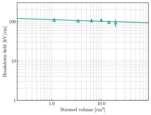
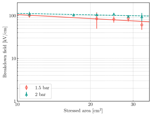
Figure 6.36: A plot of breakdown field vs. 90% stressed volume in liquid argon at 2 bar. The fit line corresponds to $E_{\mathrm{max}}=C\cdot V^{-b}$/cm³ where $C=112\pm 1$ kV/cm and $b=0.041\pm 0.043$ with $\chi^{2}=1.7$ and DOF = 3.

Figure 6.37: Comparison of breakdown performance in LAr for data taken at 1.5 bar and 2 bar as a function of stressed electrode area. Fit at each pressure was performed to $E_{\mathrm{max}}=C\cdot A^{-b}$/cm². At 1.5 bar $C=216\pm 103$ kV/cm and $b=0.31\pm 0.16$ (solid red line) with $\chi^{2}=1.4$ and DOF = 2, while at 2 bar $C=147\pm 54$ kV/cm and $b=0.11\pm 0.12$ (dashed teal line) with $\chi^{2}=1.7$ and DOF = 3.

Each data point in Figure 6.35 is the mean value of all measurements from one run taken at the same gap distance as summarized in Table 6.9. Larger electrode diameters are likely to break down at lower fields. Figure 6.35 shows the breakdown field as a function of 90% stressed cathode area using data with a purity better than 10 ppb as available in the literature. A fit to Equation 6.5 $E_{max}=C\times A^{-b}$/cm² was performed where $C=124.26\pm 0.09$ kV/cm and $b=0.2214\pm 0.0002$. Figure 6.37 shows a fit to the volume effect using data collected in XeBrA at 2 bar alone since data from other experiments are not available in the literature. A fit to $E_{max}=C\cdot V^{-b}$/cm³ was performed where $C=112\pm 1$ kV/cm and $b=0.041\pm 0.043$.

Since data in LAr in XeBrA were collected at two different pressures, Figure 6.37 compares the breakdown performance at 1.5 bar and 2 bar. Data at each pressure were fit to Equation 6.5. At 1.5 bar the slope was $b=0.31\pm 0.16$ while at 2 bar $b=0.11\pm 0.12$, so the measured slope of the breakdown dependence on the area at 1.5 bar is steeper than for 2 bar. Note that temperature inside the apparatus was changing throughout the measurements as illustrated in Figure 6.28.

6.8.3 Liquid xenon data analysis

Figure 6.38 shows a histogram of breakdown events for each electrode separation during Runs 2 and 3. Table 6.9 summarizes information about data acquired in LXe.

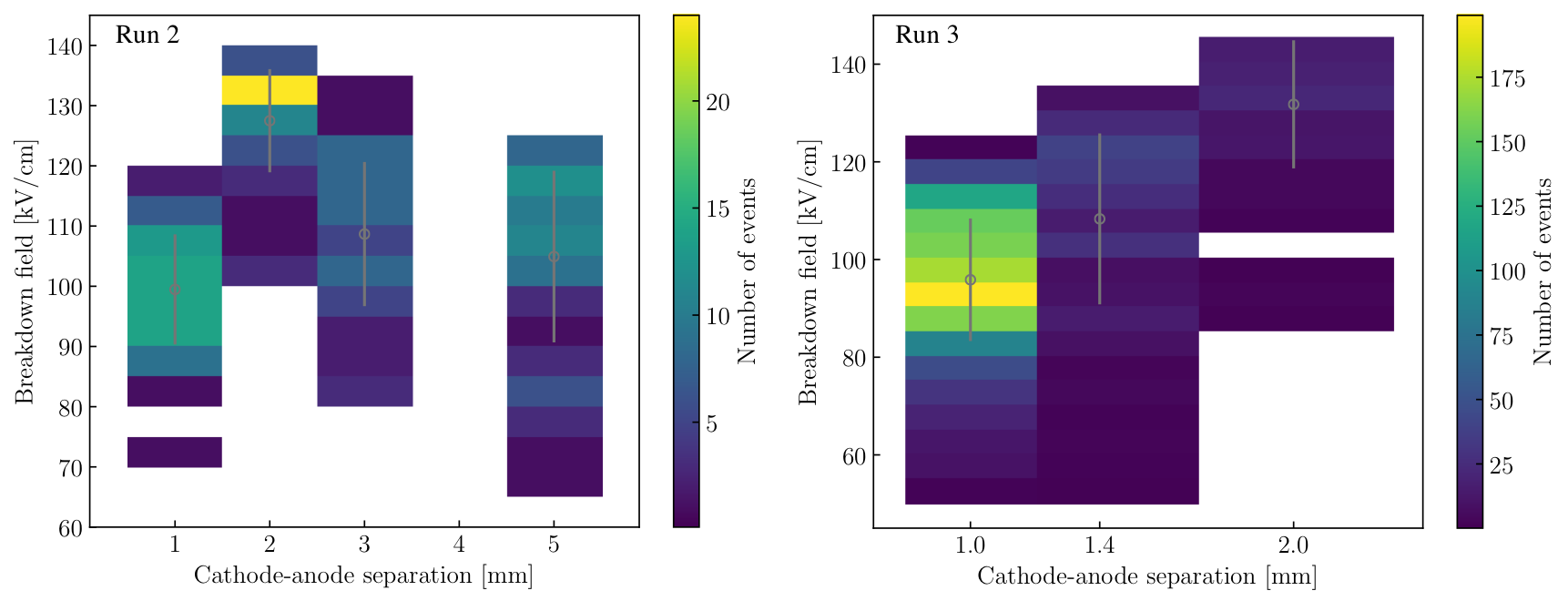
Figure 6.38: Histogram of breakdowns in LXe as a function of electrode separation. Data were taken at 1.5 bar (left) and 2 bar (right). The vertical bars indicated the standard deviation at each separation.

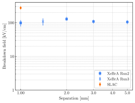
Figure 6.39: A plot of breakdown field vs. electrode separation in LXe. XeBrA’s large electrodes perform worse than the 1.5 cm diameter spheres employed in the SLAC measurement, indicating that the breakdown likely depends on another factor, such as the stressed electrode area. The SLAC result is taken from [361].

Figure 6.40: A plot of breakdown field vs. 90% stressed area of the cathode in LXe. The fit line corresponds to $E_{\mathrm{max}}=C\cdot A^{-b}$/cm² where $C=171\pm 8$ kV/cm and $b=0.13\pm 0.02$ with $\chi^{2}=6.5$ and DOF = 5. The SLAC result is taken from [361]. Also shown (not a measurement) are the expected area and the peak electric field in LZ for the largest surface cathodic surface (the cathode ring) and the electrode with the highest field, for a cathode voltage of -100 kV.

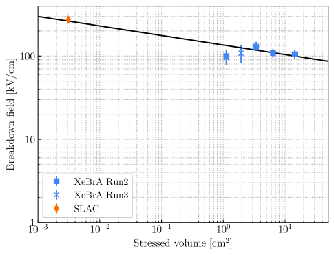
Figure 6.41: A plot of breakdown field vs. 90% stressed volume in liquid xenon. The fit line corresponds to $E_{\mathrm{max}}=C\cdot V^{-b}$/cm³ where $C=136\pm 6$ kV/cm and $b=0.11\pm 0.01$ with $\chi^{2}=10.0$ and DOF = 5. The SLAC result is taken from [361].

The data collected in Run 2 and Run 3 did not exhibit dependence on purity, so both acquisitions are included in the following analysis. The characteristic behaviors of dielectric breakdown as a function of separation, stressed electrode area, and stressed volume are shown in Figures 6.40, 6.40, and 6.41, respectively. Figure 6.40 shows that smaller electrodes perform better at equal separation in LXe. Figure 6.40 shows the breakdown field as a function of 90% stressed cathode area. A fit to Equation 6.5 $E_{max}=C\times A^{-b}$/cm² was performed where $C=171\pm 8$ kV/cm and $b=0.13\pm 0.02$. Figure 6.41 shows a fit of the volume effect to $E_{\mathrm{max}}=C\cdot V^{-b}$/cm³ where $C=136\pm 6$ kV/cm and $b=0.11\pm 0.01$.

6.8.4 Conditioning

As mentioned in Section 6.1, surface conditioning might be present during breakdown studies. Conditioning is frequently used in vacuum applications to increase the breakdown voltage of surfaces. Reference [366] saw that the breakdown voltage between the open contacts of vacuum circuit breakers immediately after manufacturing is low and shows high scatter, an effect that goes away after conditioning. Note that conditioning process will only dominate as long as the spark energy $\left(E=\frac{1}{2}CV^{2}\right)$ is low enough not to lead to pronounced conditioning damage right at the first, low breakdown value [368].

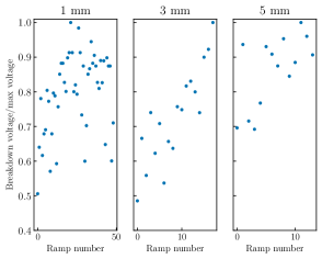
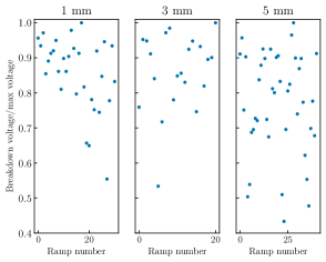
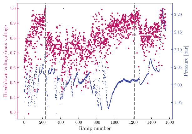
Figure 6.42: Normalized breakdown value as a function of ramp number in LAr for three different electrode separations. Data were normalized to the maximum breakdown voltage at each separation. Left: Data collected in the morning of May 26, 29, and 31, 2018, at 1.5 bar. Right: Data collection starting $\sim 0.5$ hour after the end of the data on the left. Data were collected at 2 bar.

Figure 6.43: Normalized breakdown value as a function of ramp number in LXe in Run 3. Data were collected at three different electrode separations indicated by the gray dashed lines; 1.4 mm (left), 1 mm (center), and 2 mm (right). Data at each separation were recorded without interruption. There was a half-day break between data acquisitions at 1.4 mm and 1 mm. Data collection at 2 mm immediately followed the 1 mm dataset as shown in Figure 6.29.

To observe whether any conditioning effect was present in studies with XeBrA, the successive breakdowns at three different electrode separations were plotted in Figure 6.43 for the morning (1.5 bar) and afternoon (2 bar) data acquisitions that were separated by $\sim 0.5$ hour. Due to small sample size, it is hard to draw any conclusions from the data.

More data were available in LXe during Run 3 as shown in Figure 6.43 for three different electrode separations. At each separation, the breakdown voltage was normalized to the maximum breakdown value at each separation. There was a half-day break between data acquisitions at 1.4 mm and 1 mm. Data collection at 2 mm immediately followed the 1 mm dataset as illustrated in Figure 6.29. The breakdown value appears to improve throughout data acquisition at 1.4 mm and 1 mm.

6.8.5 Comparison of liquid argon and liquid xenon data

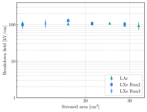
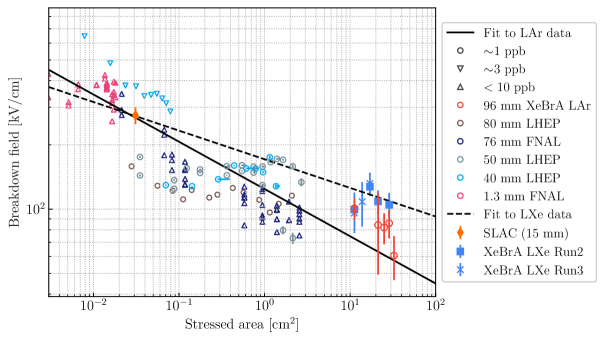
Figure 6.44: Comparison of LAr and LXe data acquired in XeBrA at 2 bar.

Figure 6.45: Comparison of breakdown field vs. 90% stressed area of the cathode in liquid argon (empty markers) and liquid xenon (solid markers). The different colors indicate the total cathode diameter used in each experiment in LAr, while the various shapes indicate LAr purity. Both LAr and LXe data are fitted to $E_{\mathrm{max}}=C\cdot A^{-b}$/cm². As stated previously, for LAr $C=124.26\pm 0.09$ kV/cm and $b=0.2214\pm 0.0002$, while for LXe $C=171\pm 8$ kV/cm and $b=0.13\pm 0.02$. Note that the plot combines data at 1.5 bar in LAr with 2 bar data from LXe.

The unique construction of XeBrA enables direct comparison of data acquired in LXe and LAr with the same geometry and electrodes. Figure 6.45 shows all data acquired in XeBrA in LXe and LAr as a function of stressed electrode area. There does not appear to be a significant difference between breakdown behavior in LXe and LAr. The literature suggests that electrode surface is one of the major factors influencing breakdown behavior, which might be supported by this result.

Figure 6.45 combines data acquired in XeBrA with other data available in the literature in an attempt to identify a trend in the breakdown behavior. Fits to Equation 6.5 as obtained in Sections 6.8.2 and 6.8.3 are also included. Comparison of data from the literature seems to suggest a steeper slope of the breakdown field with respect to SEA in LAr than for LXe. However, due to a lack of data in LXe at a wide range of areas, this comparison should be taken with caution.

6.8.6 Fitting breakdown data to a Weibull function

Assuming the power law expressed in Equation 6.6 holds in this application, fitting a Weibull distribution to breakdown distributions at various areas should yield an agreeable description of breakdown behavior $E_{max}$. Since most data at each separation was acquired in Run 3 in LXe, these data are used for this test of the weak link theory. The 2-parameter Weibull function

$$f(x) =\frac{k}{\lambda}\left(\frac{x}{\lambda}\right)^{k-1}e^{-\left(\frac{x}{\lambda}\right)^{k}}$$

was used to fit data at $x>0$, where $k>0$ is the shape parameter, and $\lambda>0$ is the scale parameter of the distribution. The resulting fit for 1 mm electrode separation is shown in Figure 6.46. The values of the fitted parameters were $k=9.6\pm 0.2$ and $\lambda=10.13\pm 0.03$.

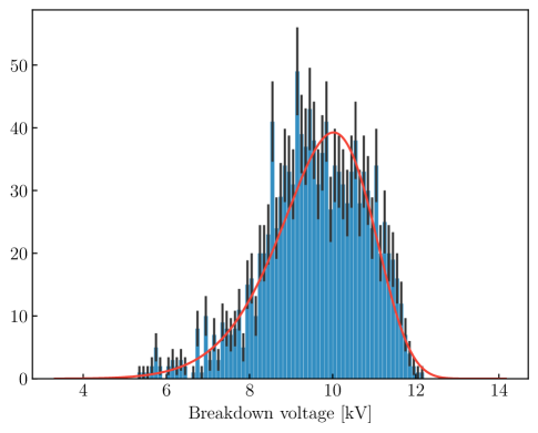
Figure 6.46: Histogram of breakdown values for 1 mm electrode separation in LXe. The solid red line shows a fit to the Weibull function with $k=9.6\pm 0.2$ and $\lambda=10.13\pm 0.03$. The $\chi^{2}$ value of the fit is 99.8, with 63 degrees of freedom.

The value of $k$ can be compared to the fit obtained from the area effect in Figure 6.40 since $k=1/b$ as stated in Equation 6.5. This results in $k=7.7\pm 1.2$. Ideally, a fit to a breakdown distribution at any electrode separation would yield a similar result. Therefore, this fit was also tried for the breakdown distributions of other electrode configurations. The distributions appeared Weibull-like. However, due to the small sample size at all other electrode configurations in both LAr and LXe, the error on the fit parameters was too large for a meaningful result. A future study with larger sample sizes and therefore more opportunity for statistical rigor could attempt to confirm the weak link theory. A fit to a Gumbel function was also attempted but did not yield good agreement with data.

6.9 Discussion

We now turn our attention to possible apparatus upgrades and future studies with XeBrA. The first data from XeBrA shed some light on the characteristics of HV breakdown in LAr and LXe. Earlier measurements performed in other liquids suggest that breakdown behavior is a complex process that depends on many parameters. Various parameters, such as electrode area, material, and surface finish, stressed liquid volume and its purity, system capacitance, and pressure might be contributing to dielectric breakdown. The contributions from those different parameters can be hard to distinguish from one another particularly since it can be hard to design electrodes or operate XeBrA in a way that does not strongly correlate with these parameters.

XeBrA’s measurement has further validated the existence of an area scaling effect for breakdown behavior. HV breakdown in XeBrA in LAr occurred at slightly higher fields than what has been predicted by previous LAr studies. This can be due to many uncontrolled or untested parameters mentioned previously. The measured slope of the breakdown dependence on the SEA in LAr at 1.5 bar was steeper than for 2 bar. This observation is consistent with the effects observed in LN and LHe [292, 350, 354]. Additionally, breakdown performance as a function of the SEA in LAr was observed to have a steeper slope than in LXe. Further studies at a wider range of areas should be conducted to confirm this observation.

The capacitance between electrodes is higher for smaller gap configurations (cf. Table 6.5), so the stored energy available for the breakdown is higher. References [369, 370] argue that an increase of the locally stored energy increases the chance of a weak initiating event to grow to a breakdown point. They correlate the increase of the local energy to the increased SEA. However, in XeBrA the capacitance between the electrodes decreases as a function of the SEA as shown in Table 6.5 and yet the area effect is observed. Additionally, the energy stored between electrodes is only a fraction of the energy stored in the HV cable, thus is unlikely to affect measurements at various electrode separations strongly. However, it is possible that the capacitance for an equivalent area is higher in the systems used for breakdown measurements at FNAL and LHEP compared to XeBrA, which could contribute to their lower observed breakdown value.

There were also data collected with a PMT in LAr for 4 mm electrode separation. These data will be analyzed to study the onset of electroluminescence prior to the spark. Furthermore, all data collected in LXe during Run 3 contain information recorded by both a picoammeter and a charge amplifier. Signals as early as 90 ms before the breakdown were seen in the charge amplifier, an example of which is shown in Figure 6.47. These data need to be analyzed to identify any patterns that might contain helpful information.

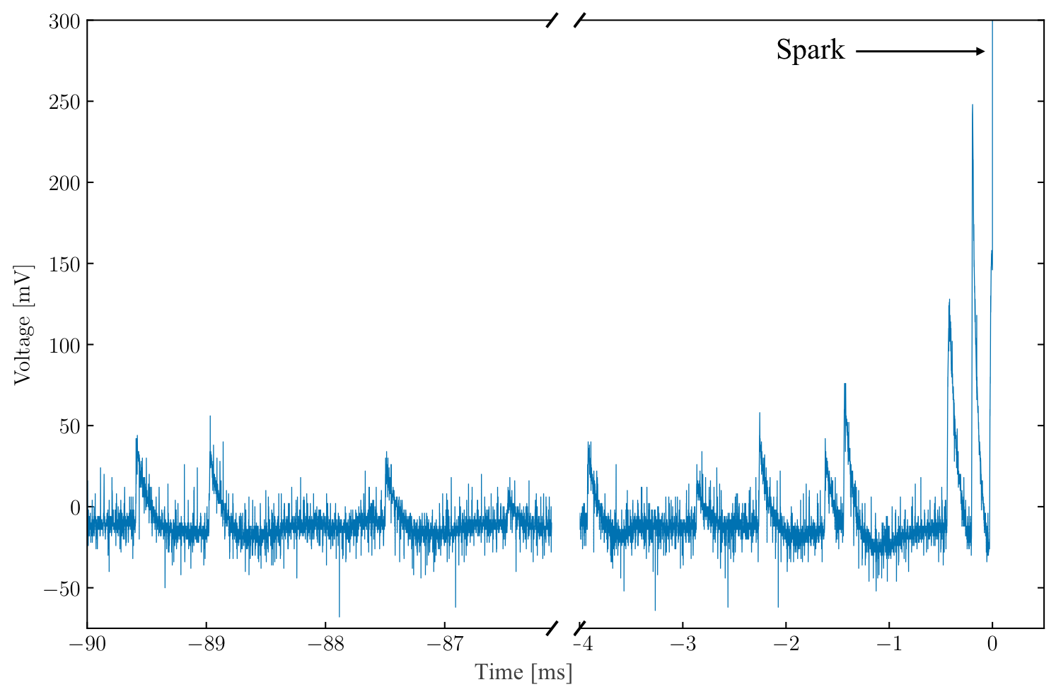
Figure 6.47: Signal recorded by the charge amplifier before one of the sparks in LXe at 1.4 mm electrode separation. Behavior between -86 and -4 ms is similar to the trace shown.

The remainder of this section discusses future upgrades in Section 6.9.1, and possible effects that could be studied with XeBrA in Section 6.9.2.

6.9.1 Future XeBrA upgrades

Operations of XeBrA in LXe revealed some necessary upgrades to the apparatus that will ensure seamless operation in the future. These can be split into two broad categories. First, some upgrades must occur prior to subsequent operations. Second, there are a few upgrades that will improve operations, but their absence does not prevent future data acquisition. This should not be considered a complete list since it is anticipated that the upgrades needed for the apparatus will evolve through time as we gain a better understanding of the breakdown behavior.

Near-term

Most imminently, the broken heat exchanger needs to be re-welded and pressure tested. Additionally, the ceramic spacers of the purity monitor need to be cleaned. A few other minor fixes include installing a new power supply to increase the heat delivered to the heat exchanger and improving the thermal coupling between the RTDs and the apparatus. Attaching RTDs to breadboards was a mistake since the breadboards made it very hard to achieve proper thermal contact of the RTD with the apparatus.

Long-term

The latest data acquisition in LXe revealed that a small amount of xenon could be frozen near the HV feedthrough, which suppresses unwanted bubbles during data taking. However, this approach cannot be used for data collection in LAr due to a lower freezing temperature. Instead, a small heater could be installed directly in the LAr space. Turning the heater on would cause a steep increase in pressure, making the apparatus temporarily bubble-free for data taking. This approach is similar to adding gas from the bottle as was done in this work but does not require the addition of gas into the apparatus.

Breakdowns near the power supply’s maximum of -75 kV did not always occur between the two electrodes. Instead, the breakdown sometimes took place between the air-vacuum epoxy HV feedthrough and the ISO100 spool at ground. In order to measure the breakdown between electrodes near this -75 kV threshold, the ISO100 port should be enlarged. This will reduce the value of electric fields near the feedthrough, thus diminishing this issue.

A two camera system is being developed to monitor the location of the spark to improve understanding of the spark development. One camera will be installed at each of the two viewports. This will enable a 2D position reconstruction of the spark to determine whether the breakdown occurs within the 90% SEA and if the location varies between each spark. This should improve the understanding of the stochastic nature of the breakdown and indicate whether the weak link theory is appropriate. It will also clarify whether using 90% SEA is appropriate or if a larger area should be used, similar to study [374]. Furthermore, a high-speed camera with a frame rate of 1,000 fps or better could be installed at one of the viewports to document the development of the breakdown in xenon. The estimate for the camera frame rate is based on a similar study performed in LAr [314].

6.9.2 Future possible studies with XeBrA

As discussed in Section 6.1, there are many parameters suspected to affect dielectric breakdown in liquids. XeBrA can be used to attempt to explore many of those in the future.

Electrode material and surface finish

Since the electrodes in XeBrA can be easily changed, electrodes from various materials could be manufactured, and their performance tested. Apart from different materials, effects caused by various surface finishes can be studied to better understand breakdown performance. A high-pressure rinse could be tested as a method to achieve a very smooth surface finish. It has been observed to improve electrode performance in other applications [398, 399]. Power washing involves using high pressure $\left(\geq 1200\,\mathrm{psi}\right)$ ultrapure water with resistivity $\geq 18\,\mathrm{M\Omega/cm}$. The procedure needs to be performed inside a clean room to maintain the electrode cleanliness.

Electrodes can also be coated with various materials. Reference [360] examined performance of coating SS electrodes in latex. This improved the performance of the electrodes but only until the first breakdown. In an upcoming test, XeBrA will test electrodes with a passivated surface to inform the design of the LZ detector’s cathode surface. Passivation causes some of the chromium in the SS to oxidize and form a layer of $\mathrm{Cr_{2}O_{3}}$ on the material’s surface. This has been found to improve the breakdown resistance of electrodes by suppressing the field emitted electrons [400]. However, in pulsed HV applications, it has been observed that once a hole develops in the coating, its performance will decrease. We want to confirm whether the performance of the passivated surface worsens after the first breakdown prior to installing such surfaces in LZ.

Additionally, to minimize surface roughness, a layer of graphite or other conductive material could be deposited to ensure a smooth electrode structure, which might improve electrode performance. Graphite dispersed in distilled water, known as aquadag™, could be used. After application, once the surface has dried, aquadag leaves a conducting layer of pure graphite.

Effects of different kinds of impurities

There is evidence that impurities affect breakdown in LAr. However, no such measurement has been done in LXe. Additionally, the effect of impurities on electron lifetime in LXe has not been well described. Since XeBrA contains a purity monitor, a known amount of various impurities could be introduced to the system to study their effect on dielectric breakdown and electron lifetime. This is predicated on the assumption that XeBrA can reach purity levels that are measurable with the existing purity monitor design, which is not yet the case but should be achievable.

Other

More data should be collected to determine whether the value of breakdown is indeed correlated with pressure, as indicated by XeBrA’s measurement in LAr. Since at the current configuration XeBrA cannot accommodate larger electrodes, smaller electrodes can be installed to evaluate breakdown at a broader range of SEA to identify breakdown trends in LXe. Furthermore, larger sample sizes of breakdown data at each electrode separation could be used to evaluate the validity of the weak link theory. Additionally, the effect of muons on breakdown could be examined. Muons passing through the active volume will ionize the liquid, potentially creating a region with enhanced breakdown probability.

6.10 Conclusion

XeBrA is the first experiment to provide systematic studies of dielectric breakdown in LAr and LXe at electrode areas greater than $3\,\mathrm{cm^{2}}$. Results from XeBrA obtained in LAr and LXe with the same electrode also enable direct comparison of breakdown behavior in those two noble liquids. These early results indicate that a steeper dependence on the SEA may be expected for breakdowns in LAr than in LXe. However, the validity of the measurement needs to be confirmed with a more extensive dataset in LXe. Results from XeBrA also indicate a stronger area dependence of breakdown field at lower pressures in LAr, an effect that is worth future examination.

This study also attempted to fit a single breakdown distribution to examine the validity of the weak link theory prediction. A single data point agreed with the prediction. However, a bigger sample is needed to evaluate the validity of the Weibull hypothesis.

Further studies will also incorporate information acquired by a picoammeter and a charge amplifier connected to the ground electrode during data acquisition. Additionally, PMT data will be examined to study the onset of electroluminescence prior to a spark.

Given the complex nature of dielectric breakdown, it is difficult to predict whether the results from XeBrA can be extrapolated for application in LZ. Nevertheless, the current results from XeBrA bear good news for the LZ detector since the predicted breakdown strength in LXe is well above the LZ design parameters. Investigation of a diverse set of parameters over a wider range of areas will need to be performed to better understand the contribution of various parameters to the dielectric breakdown probability. The results presented in this chapter started this investigation. Future studies with XeBrA will further improve our understanding of breakdown behavior in LAr and LXe.

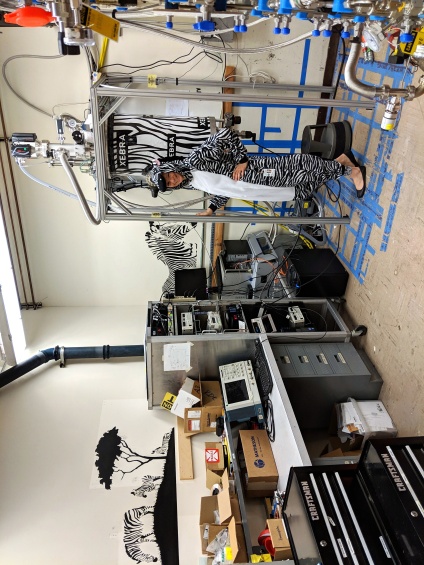
Figure 6.48: Z/XeBrAs.

Appendix A LZ Equity & Inclusion

Only about $20\%$ of doctoral degrees in physics are awarded to women as illustrated in Figure A.1, and one factor may be that women are very likely to experience sexism and microaggressions in their career [401]. In fact, research shows that $20\%$ or more of undergraduate and graduate female science students have experienced sexual harassment from faculty or staff [402]. The LZ Equity and Inclusion (E&I) committee was formed to help address these problems more broadly. It attempts to address these problems within the scope of the LZ collaboration and to create a model for future collaborations. This is not only a moral imperative but also a strategic investment for the collaboration both in attracting new talent and in preventing attrition due to unsavory working conditions for women and minorities. Solving issues faced not only by women, but by minorities in general, creates a healthier and more productive [403] working environment for all collaboration members that enables the LZ collaboration to achieve its highest potential.

The LZ E&I working group was formed in spring 2017 after it was realized that some of the issues mentioned above have surfaced within the LUX collaboration in the past and we wanted to provide a safeguard to the even larger, more diverse LZ collaboration. Harry Nelson, an LZ professor, and I attended a workshop about the Impacts of Sexual Harassment in Academia organized by the US National Academy of Sciences, Engineering, and Medicine in June 2017 at UC Irvine. This committee very recently released an extensive report [402], featuring fifteen concrete recommendations on improving the current climate - many of which were adopted by LZ prior to the release of this report on the recommendation of the E&I committee.

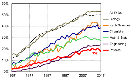
Figure A.1: Fraction of U.S. doctoral degrees awarded to women in Science, Technology, Engineering, and Mathematics (STEM) fields. There were 352 doctoral degrees in total awarded to women in 2017. Overall, more doctoral degrees were awarded to women than to men. Women received the majority of doctoral degrees in popular fields, such as health sciences (70.3%), education (68.8%), and social and behavioral sciences (61.1%) [404]. Figure from IPEDS and APS [405].

One of the recommendations asserts that academic institutions should consider sexual harassment to be equally important as research misconduct in terms of its effect on the integrity of research. Academic misconduct is a broad umbrella topic with a lot of complexity and nuance for which institutions have spent years implementing systems and policies in an attempt to protect academic integrity. Similarly, sexual harassment likely cannot be solved with one simple, black-and-white rule change, but instead requires a change of climate and an entire paradigm shift. It is important to avoid thinking about this problem with a too narrow mindset and to set expectations corresponding to a long and nuanced journey toward excellence.

Efforts to reduce sexual harassment and discrimination in the workplace have been ongoing for decades; laws have been put in place addressing these issues, albeit not very successfully. In particular, Title IX, that prohibits discrimination on the basis of sex in any federally funded program, and Title VII that prohibits employers from discriminating based on sex, race, color, national origin, and religion, spurred the creation of policies and sexual harassment training in order to comply with the law and avoid liability. While laws, regulation, and policy frequently reflect a real need for change, the specific implementations can cause their efficacy to vary wildly or even induce harm. Indeed, research suggests that voluntary sexual harassment or diversity training has proven to be effective, while mandatory training can have no or even adverse effects [406]. Furthermore since academia relies so heavily on its hierarchical structure with junior members often needing recommendations from their superiors to advance their careers, reporting any harassment can be impractical due to worries of retaliation. Reporting has even been shown to harm the victims instead of providing the much-needed support [407] and frequently the institutional response shields the star faculty and protects the institution from liability rather than looking after victims [408].

Therefore the LZ E&I committee set out to implement a more thoughtful and comprehensive approach to address both sexual harassment and a broader set of workplace-related issues. These issues include anything that might prevent people from joining or staying in the collaboration and range anywhere from implicit biases and stereotype threats, hostile workplace, and sexual misconduct, to microaggression, inappropriate jokes, being spoken over during meetings, paper authorship issues, and beyond. Our attempts to address all of these issues started in the spring of 2017 in a small group that included me, Dan Akerib, and Harry Nelson, later also joined by Rachel Mannino. We met weekly, consulted many researchers in psychology, sociology, and other physicists with experience in similar projects, and ultimately presented a comprehensive set of policies to the LZ collaboration in March 2018. Section A.1 chronicles that year of hard work and describes the actions and policies that resulted therefrom. In addition, Section A.2 summarizes the findings of a side project that delves into the benefits of double-blind review for academic publications as it presents yet another piece of the puzzle that has been shown to benefit minorities.

A.1 LZ policies

The goal of the policies presented to the collaboration was to develop positive, aspirational procedures and for the collaboration as a whole to make a positive statement that a fair working environment is an important factor toward delivering great science. Since membership in the LZ collaboration is a privilege and should be approached as such, the policies strive to set expectations for a professional environment protecting equal research grounds for everyone. Given the breadth of in-person interactions within the LZ collaboration at a wide variety of locations throughout the world, the policies address the specific needs of the collaborations acknowledging different cultural backgrounds of collaborators and the variety of interactions encountered during both remote and in-person interactions. Unlike universities and research labs, LZ is not a legal entity (and therefore cannot be sued), so the policies developed are not overly legal and restrictive, but rather serve to inform collaborators of resources available at their home institutions and provide additional support.

The documents presented here were co-authored with the Equity & Inclusion committee and adopted as official LZ policies by the LZ Institutional Board (IB) in March 2018. They were presented to the LZ collaboration at the inaugural Equity & Inclusion plenary session at a collaboration-wide meeting in Coimbra, Portugal in April 2018. These efforts generated very positive feedback, and following the Coimbra collaboration meeting, the Equity & Inclusion committee grew to 15 members and proceeded to nominate its first two Ombudspersons.

There were three documents adopted by the LZ collaboration, along with a modification to the LZ governance document that made the E&I committee an official part of the collaboration. As the name suggests, the LZ Equity & Inclusion Scope of Activities presented in Section A.1.1 defines the charge of the committee. The LZ Code of Conduct is an aspirational 1-page long document that sets expectations for collaborators regarding their behavior and scientific misconduct as presented in Section A.1.2. It also links to the LZ Institutional resource list, maintained by the E&I committee, that features an up-to-date list of resources available at each of the collaborating institutions.

LZ also appointed two ombudspersons. The role of the LZ Ombudspersons is to help and refer people who come forward with any issues that might arise within the collaboration as outlined in Section A.1.3. Information shared with the LZ Ombudspersons is assumed confidential within the collaboration, hoping to encourage members who might worry of retaliation otherwise. The ombudspersons are also expected to identify systemic problems and organizational issues within LZ and assist in finding solutions as needed. At any time there are two ombudspersons from different institutions serving on a 2-year staggered term. This avoids potential interference with any mandatory reporting rules that might be in place at either of the ombudspersons’ institutions.

Last, but not least, every in-person LZ collaboration meeting now features a plenary and a parallel session on diversity-related topics to encourage discourse within collaborators on this topic, as discussed in Section A.1.4.

The E&I efforts are expected to change throughout time as we learn more and better understand the best practices for promoting a genuinely inclusive working environment. The E&I committee also considered deploying a collaboration-wide survey, such as the ARC3 Campus Climate survey [409]. This effort was postponed due to a worry of ability to provide anonymity to women who might have experienced harassment within the collaboration because of potentially low survey response rate (and due to the low number of women in the collaboration in general), lack of experience analyzing this type of data, and funding reasons. However, the survey should be considered in the future in order to acquire data to help track the impact of the committee’s efforts. Other possible future projects include a journal club on the topic of diversity, so that committee members remain up-to-date on the most recent advances in the field, establishing a mentoring program for graduate students, postdoctoral fellows and junior faculty within the collaboration, and more. Since there are a few other physics collaborations with ombudspersons, the committee is also considering connecting all those ombudspersons to facilitate sharing insights and leverage each other’s experiences in solving problems that come up. Depending on the success of the E&I efforts within LZ, the committee might also consider helping other physics collaborations set up their E&I ventures.

A.1.1 LZ Equity & Inclusion Scope of Activities

1. Introduction: This document describes the LZ Equity & Inclusion Committee (EIC), which was established by the LZ Institutional Board (IB) as described in the LZ Governance Document. The committee aspires to ensure that the climate in the LZ collaboration is positive, respectful, and supportive of all its member. It will work towards this goal by providing resources, establishing and managing the role of LZ ombudspersons, developing a Code of Conduct, organizing talks and other educational activities at collaboration meetings, and occasionally providing assessment and advice on the climate to the collaboration leadership.

2. Code of Conduct: The EIC will submit to the IB for approval a Code of Conduct to set out expectations for behavior among collaborators across the variety of circumstances that they may encounter. By its very nature, the Code is an aspirational document and aims to encourage positive behavior towards all members of the collaboration. The Code will be described in a separate document and is subject to approval and modification by the IB. All active members of the collaboration must agree to follow the Code.

3. Ombudspersons: The EIC will propose 2 candidates for the role of ombudspersons appointed by the LZ Spokesperson to provide collaboration members with a confidential resource to turn to if they encounter situations with other members of the collaboration that are counter to the Code of Conduct, or other troubling situations in which they require support, including but not limited to sexual harassment, hostility, coercion, or other negative behaviors. The role and structure of the ombudspersons are described more fully in a separate document to be approved by the IB. At large gatherings, such as collaboration meetings or analysis workshops, the EIC and ombudspersons will appoint a meeting ally in cases where the ombudspersons are not in attendance in order to provide in-person support.

4. Resources: The EIC will promote a respectful environment for all collaboration members during collaboration interactions and maintain a resource page on the LZ Twiki. This will include general equity & inclusion resources as well as resources specific to each member institution. For example, each US educational institution employs a Title IX coordinator to enforce sexual harassment prevention, and other policies pertaining to hostility, coercion and other prohibited practices, as well as providing support to victims. Many institutions also maintain an ombudsperson or similar to provide a range of support, including confidential support.

5. Collaboration Meetings: The EIC will be allocated plenary time at each collaboration meeting to program at its discretion. Such programming may include outside speakers on matters pertinent to the committee’s work, occasional presentation and discussion of the Code, resources, ombudspersons, or other matters aimed at informing the collaboration within the EIC’s scope.

6. Assessment: The EIC may occasionally conduct surveys of the collaboration to assess the needs of the collaboration within the committee’s scope. These will be conducted in consultation with the collaboration leadership and reported to the IB and the collaboration. The committee also welcomes broad input from the collaboration on any matters within the committee’s scope on ways to maintain and improve a positive and supportive culture.

7. Structure: The EIC committee will consist of members from all ranks and titles of the collaboration, but will include at least one graduate student and one postdoc member. The Spokesperson is an ex-officio member. The committee will be structured as a committee of the whole. The committee shall meet before every collaboration meeting and more frequently as needed.

A.1.2 LZ Code of Conduct

The LZ Code of Conduct [410] aspires to strengthen trust and mutual respect among collaborators to foster an inclusive collaboration environment supportive of sound scientific research. Every LZ member should read the Code, and follow both its spirit and letter, always bearing in mind that each of us has a personal responsibility to incorporate, and to encourage others to incorporate, the principles of the Code into our work.

The LZ collaboration is committed to a supportive work environment, where everyone has the opportunity to reach their fullest potential dedicated to the advancement, application, and transmission of knowledge through academic excellence. This policy applies to all interactions between LZ collaborators although the formal policies of individual institutions take precedence. Some examples of interactions include collaborators’ in-person, virtual, or phone interactions, or any social or professional gathering both at formal institutions and during social events associated with the collaboration. LZ collaborators should act in concordance with a professional culture that fosters respectful interactions and a safe environment free of harassment, intimidation, bullying, bias, discrimination, or mistreatment of any kind. LZ collaborators must refrain from any actions or statements that denigrate other collaborators on the basis of personal characteristics or beliefs. This includes, among other actions, intimidation, disruptive, or harassing behavior of any kind, sexual or crude jokes and comments, offensive images, or any unwelcome physical contact. Please be aware that behaviors and language acceptable to one person may not be to another.

The conduct of LZ collaborators must be based on dedication to the highest scientific and technical standards. Collaborators are expected to perform research in a well documented and ethically sound manner. Falsification of data or results, plagiarism, violations of the LZ Publication Policy, taking credit for others’ work, or any other scientific misconduct will not be tolerated.

Unacceptable conduct may warrant further action. For example, code violations could result in consequences, up to sanctions by the IB according to the LZ Governance Policy.

If you have a question or ever think that one of your colleagues or the collaboration as a whole may be falling short of our commitment, don’t be silent. Your collaborators and leadership need to hear from you. You may report any misconduct to your supervisor, collaboration’s spokesperson, ombudspersons, meeting allies, or the Title IX or diversity officer of either your institution or the institution where the incident took place (see the LZ institutions resource list for details). LZ does not tolerate retaliation against any collaborator who reports or participates in an investigation of a possible violation of our Code, policies, or the law.

The intention of this Code of Conduct is to ensure that the collaboration is a welcoming place for everyone so if you see something that you think isn’t right – speak up!

A.1.3 LZ Ombudspersons Guide

This document summarizes reach and responsibilities of the LZ Ombudspersons [411]. Further information about the Ombudspersons reach and responsibility can be obtained from the International Ombuds Association.

The LZ Ombudspersons provide confidential, informal, independent, and impartial assistance for any LZ collaborators on matters pertaining to collaboration values, including dispute resolution services. The LZ Ombudspersons are available to LZ collaborators who are experiencing conflicts or disputes as part of their LZ activities rather than with problems internal to an academic institution, which can usually be mediated by the appropriate offices in that institution (including the institutional ombudsperson). The LZ Ombudspersons will work together with the members who consult them to identify options for managing and resolving disputes and conflicts. This includes providing advice and support, finding out information about, or referring individuals to, appropriate resources, and facilitating mediation.

An LZ Ombudsperson may report systemic issues or patterns of concern in the collaboration to the LZ Equity & Inclusion committee (EIC) and the Spokesperson but may do so only without disclosing individual names or other aspects that would identify parties. Confidentiality is a privilege of the LZ Ombudspersons. The only circumstances that there may be an exception to confidentiality is if the Ombudsperson is concerned by an imminent risk of serious harm, or if required by law in the applicable jurisdiction to anonymously report credible evidence of fraud, waste, or abuse concerning the use of government funds. Please note there is no recognized privilege, similar to attorney-client privilege, for ombudspersons in U.S. courts.

To avoid mandatory reporting requirements of an ombudsperson to their home institution (where their confidential role may not be recognized), LZ shall have two Ombudspersons from two different LZ institutions; LZ scientists can contact whichever Ombudsperson they feel is appropriate. The LZ Ombudspersons should not have any other collaboration leadership role that may compromise their impartiality or confidentiality.

The Ombudspersons are required to become familiar with the Title IX rules of their institution (ideally by meeting with their institution’s Title IX or Diversity officer), with other code of conduct policies at their institution, and with the organizational structure of the LZ collaboration. This will allow them to provide current information about services, programs, policies, and procedures. By having two LZ Ombudspersons, it is expected collaboration members will have access to an ombudsperson not at their home institution, providing them with a confidential resource outside of their research group. Additionally, for matters arising within an institution, LZ members are encouraged to seek out the ombudsperson or other resources at their home institution.

If neither one of the Ombudspersons is able to attend an in-person collaboration meeting, the Ombudspersons and the EIC will appoint two “meeting allies” for the event. These persons will temporarily act as Ombudspersons for the duration of the event.

To prevent recurring events and maintain institutional memory given the 2-year term of the Ombudspersons, they are expected to keep a log. Each ombudsperson may share the identity of the complainant with other ombudspersons (current and future) only with explicit permission of the complainant. The EIC will explore the use of other ombuds tools, such as Callisto, but will employ such only after appropriate consultation with the IB and with full knowledge by the collaboration.

A.1.4 LZ collaboration meeting plenary presentations

Research shows that discussion of diversity can have a very positive effect on retaining female (and potentially minorities in general) in physics [412]. Therefore an essential part of the adopted policies are the in-person presentations at the bi-annual collaboration-wide meetings, which are intended to enhance collaborators’ knowledge on a diversity topic and to encourage a discussion on the topic. The first plenary session in Coimbra in April 2018 was devoted to the introduction of the LZ E&I efforts. The second plenary session at Brandeis University in July 2018 hosted Prof Frank Dobbin, a sociology researcher from Harvard University, whose talk was very well received and set high expectations for future meetings.

The parallel sessions enable the Equity & Inclusion committee to gather feedback from the collaboration members on topics the committee is working on at the moment and provide an excellent opportunity to discuss thought-provoking diversity manuscripts in a smaller group than the plenary session. The well-attended, inaugural parallel session at Brandeis University featured a presentation highlighting recommendations relevant to the collaboration from the report on Sexual Harassment in Academia [402] and a discussion about the shared collaboration housing in Lead, South Dakota.

A.2 Case for the double-blind peer review

The text below was also published in [413].

Peer review is a process designed to produce a fair assessment of research quality prior to the publication of scholarly work in a journal. The process consists of sending a candidate work such as a journal article to a number of similarly qualified professionals for feedback and informs publishers of academic journals whether a work should be accepted or rejected. Peer review is used as a gold standard in assessing manuscripts and is essential for academics since tenure, grant applications, and many other career-related decisions are based upon the quality of their work and publications making the stakes are high. Most journals today use a single-blind review method, in which the reviewer’s identity is concealed to the author of the article, but not vice versa. However, some journals use alternative review strategies [414, 415], such as double-blind review, where both the author’s and the reviewer’s identities are concealed, or open review [416, 417], where all information is public.

It is well known that implicit biases influence people’s decision making, but ideally, decisions regarding the importance of scientific contributions would be free of these biases. Nevertheless, demographics, nepotism, and seniority have been shown to affect reviewer behavior suggesting the most common, single-blind review method (or the less common open review method) might be biased [418, 419]. Blinding both the author’s and reviewer’s identity can reduce exposure to extraneous information thus bypassing bias and optimizing decision making. Although this article focuses on academic journals, blinding has the potential to affect decision making in many areas: it has been demonstrated that blinding applicants in the first stages of grant applications reduces biases related to researcher’s characteristics [420] and blind musical auditions have significantly increased the number of women in symphony orchestras [421]. Moss et al. also showed that blinding the gender of job applicants can reduce unconscious and unintended bias [422].

Many characteristics can be subject to biases that might skew the reviewer’s decisions as discussed below. For example, there is substantial evidence for biases in favor of famous authors and world-renown institutions, but there are only limited data on the impact of review on women and minorities. Budden et al. found that switching to a double-blind review in an ecology journal led to a small increase of female first author paper [423]. However, these findings were later rebutted [424, 425, 426] and this increase was attributed to a proportional increase of women in the workforce overall. Journal of Neurophysiology also found no gender bias in their publications, but carefully notes that at the time of the analysis 5 out of 9 members of the editorial panel were women and only 191 of 713 submissions (26%) were from women-first authors [427]. Blank found that although women perform slightly better under a double-blind system, the data were statistically not significant [414]. It should be noted that women published only 150 out of 1,223 analyzed papers (12%). Other journals also found author identity did not influence acceptance rates or quality ratings in review [428, 429].

Conversely, after the Modern Language Association (MLA) switched to double-blind review a substantial increase in acceptances for female-authored publications was observed, eventually comparable to that for men [430]. Tomkins et al. did not find any gender bias in their study of the review process in computer science using their data alone, but combining their results with previous studies showed a statistically significant gender effect bias [431]. Studying this topic, Helmer et al. demonstrated that women are currently underrepresented in the peer review process and that editors of both genders preferred same-gendered authors [432]. This behavior highlights the need to employ review methods that combat subtler forms of gender bias in scholarly publishing.

Despite the mixed data regarding the effect of double-blind review on gender bias, it has been demonstrated that double-blind review can mitigate biases arising from researcher’s popularity or location. Tomkins et al. found that single-blind reviewers were significantly more likely to recommend for acceptance papers from famous authors and top institutions [431]. Moreover, if reviewers knew the author’s identity, they disfavored authors that were not sufficiently embedded in their research community [433]. Link discovered that in a medical journal the location of the authors mattered as US reviewers ranked US papers much more favorably compared to the non-US ones [419]. Additionally, Blank found that under a double-blind review acceptance rates were lower and reviewers were more critical [414]. This suggests that a double-blind system might lead to more critical feedback from reviewers and a mix of accepted papers from more diverse authorship.

It should be noted that before a manuscript reaches the review stage, journal editors who have access to authors’ information reject many, sometimes most, of the papers submitted to a journal before a reviewer can see them. While motives will differ between editors and reviewers, there is no reason to assume that editors are less susceptible to bias than reviewers [434]. This issue could be overcome with the use of double-blind review since editors would also lose access to authorship information.

A common concern for double-blind review is the identification of author or institution from self-citations, nature of work, or personal connections [435, 436]. Hill and Provost found that even using the best method to identify authors based on discriminative self-citations, authors were identified correctly only 40-45% of the time suggesting that even in the worst-case scenario blinding is successful most of the time [437]. Other arguments against double-blind review such as administrative inconvenience, posting articles to other websites prior to their publications, possible conflicts of interest, or tradition can be overcome [438]. In physics, the issue of identification becomes significantly more relevant due to the high number of large international collaborations of various scales ranging from dozens to thousands of members. Often, publications from these collaborations will be trivial to identify. However, it is also unlikely they will suffer any disadvantages while the double-blind review could still benefit researchers who might currently be affected by the biases in the review process.

A scientist’s career should not be influenced by stereotypes, but rather depend on an individual’s proven track record to perform. Reviewers are people too, and since biases can affect anyone the community should strive toward a peer review system that makes its best effort to overcome the susceptibility to bias. Current research suggests that double-blind review reduces bias that might arise while assessing the quality of the research presented in a manuscript, without imposing any major downsides. Double-blind review offers a solution to many biases stemming from author’s gender, seniority, and institution and should be a foundation of any journal that strives to evaluate author’s work strictly based on the quality of the research presented in the manuscript.

Appendix B A very brief introduction to fittings

There are many different types of fittings one encounters during a day in a lab. The world of fittings can be very confusing and overwhelming at first due to similar names and very slight differences in use. This appendix attempts to offer a brief, high-level overview of standard fittings one might encounter in a lab that is concerned with noble (and not so noble) gasses and liquids.

An overview of the fittings and their applications is provided in Table B.1. For clean noble gasses, all-metal connections such as Swagelok VCR (Section B.1) or CF (Section B.2) should be used whenever possible. Other connections that can be encountered when working with clean noble gasses at higher pressures are Swagelok tube fitting (Section B.4) and CGA 580 cylinder connections (Section B.7). For vacuum application CF (Section B.2), KF (Section B.3), or Swagelok VCR (Section B.1) are among the most common connections available. The NPT standard (Section B.5) is most often used for water connections.

Unfortunately, it is very hard to build a system that uses a single fitting standard, but parts that convert between nearly all types of fittings discussed in this appendix can usually be purchased. If they cannot be purchased, they can usually be custom welded to create a leak-tight connection. All parts should be cleaned with lint-free wipes and isopropyl alcohol or ethanol before use. If the parts are very dirty, a sonicator can be used as well.

The information presented in this section is based on lab experience and documentation available on the websites of Swagelok and Kurt J. Lesker companies.

Fitting type	VCR	CF	KF	Tube	NPT	Flare	CGA580
Section	B.1	B.2	B.3	B.4	B.5	B.6	B.7
All-metal seal	Y	Y	N	Y	N	Y	Y
Durability of seal	Y	Y	Y	N	N	N	Y
Leak tight	Y	Y	Y	Y	Y	Y	Y
Vacuum	Y	Y	Y	Y	Y	Y	Y
Positive pressure	Y	Y	N	Y	Y	Y	Y
Recommended for cryogenic	Y	Y	N	Y	N	N	N
Recommended for baking	Y	Y	Y	Y	N	N	N

Table B.1: Overview of fittings and their application. Note that this presents the most common uses of each fitting. For example, KF can be used with a metal O-ring thus create an all-metal, bakeable seal. Consult the individual sections for details.

B.1 Swagelok VCR^®

Swagelok Vacuum Coupling Radiation (VCR) fittings offer a high purity metal-to-metal leak-tight seal from vacuum to positive pressures. VCR fittings are particularly useful for clean gas system design due to their compact size and a wide variety of parts available. Similarly to other metal-to-metal seals, VCR can be baked to remove internal contamination. A variety of VCR face seal glands and bodies is available with controlled surface finishes and specially cleaned to meet ultrahigh purity system requirements. The most common sizes of fittings are 1/4 in, 3/8 in, and 1/2 in, referring to the outer diameter (OD) of the tubing. Fittings are also available for 1/8 in, 5/8 in, and 1 in tubing but with a smaller selection of compatible parts and adaptors, so where possible should be avoided.

Two glands compressing a gasket make the seal of a VCR assembly. The two glands are pushed together by either a male nut or a male body hex and a female nut or a female body hex as shown in Figure B.1. As the two nuts are tightened, the glands crush the gasket, which forms a leak-tight seal.

There are several types of gaskets available made from stainless steel (SS), silver-plated SS, copper, and nickel. Additionally, gasket retainers are available to make insertion of gaskets between the glands in awkward places easier. The use of silver-plated SS gasket is recommended for uses in noble gas systems, while the use of pure SS gaskets should be avoided. The unplated SS gasket is likely to form a permanent seal with the glands by cold welding making the connection inseparable. For the same reason, the female threads are silver plated to prevent galling, ensuring smooth, consistent assembly. Therefore, chemical processes such as electropolishing and passivation should be avoided to prevent the removal of the plating.

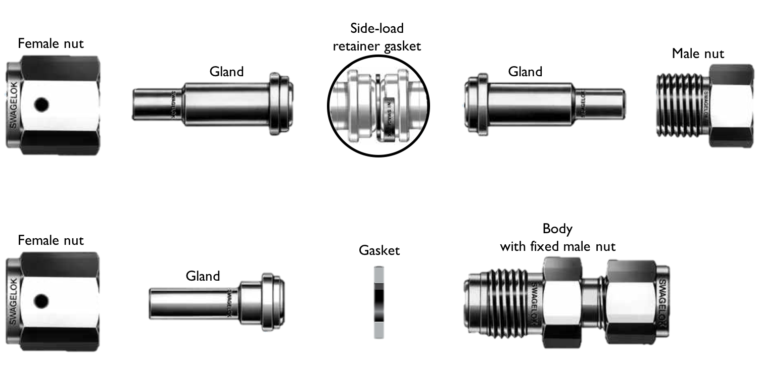
Figure B.1: Illustration of components needed for VCR assembly. Top: Rotatable male and female nuts with a gasket retainer are used to create a seal. Bottom: Fixed hex male body and a rotatable female nut are used to create a seal. Figure modified from [439].

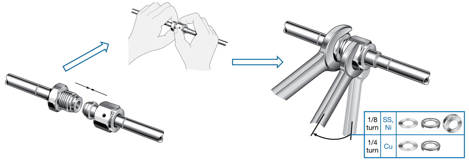
Figure B.2: Illustration of steps for Swagelok VCR assembly. Figure modified from [439].

To make a VCR connection, the mating surfaces should first be inspected to ensure they are free from scratches. Lint-free gloves should be worn during VCR assembly since the slightest fingerprint or other residues can significantly influence the quality of the seal. A gasket is then installed between the two glands as shown in Figure B.2. To make the connection, at least one of the nuts needs to be free to spin, and non-rotatable nuts must not move. The two parts should then be threaded together until finger-tight. The final seal is made by using two wrenches and tightening them by 1/8 turn (45 degrees) when using a silver-plated SS gasket. Beware of overtightening the connection as it will cause permanent damage to the sealing surface as illustrated in Figure B.3. VCR connections can be remade; however, a new gasket has to be used for each new connection. The male and female parts should be well aligned before tightening to avoid excessive strain, which can prevent the seals from being leak-tight.

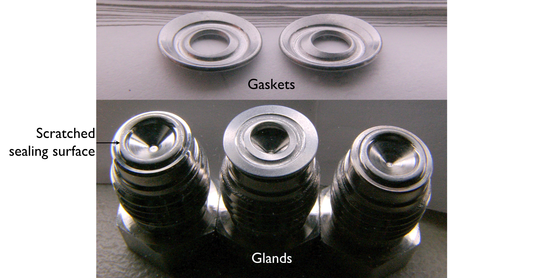
Figure B.3: Failed VCR connections. Overtightening the connection causes damage to the sealing surface and may cause a permanent connection between the gasket and the gland. Photograph from Ethan Bernard.

Each female nut has two test ports for easy leak testing. The VCR fitting design can achieve a maximum leak rate of $4\times 10^{-9}\,\mathrm{cm^{3}/s}$ with silver-plated and copper gaskets, and $4\times 10^{-11}\,\mathrm{cm^{3}/s}$ with unplated gaskets [440].

Note that VCR is a registered trademark of Swagelok company. Other VCR-like products can be purchased, but the fittings may not necessarily be compatible across different brands. Generically, the glands are called “face seal.”

Additionally, an orbital welding system can be purchased from Swagelok to produce precise gas tungsten arc welds and used with VCR face seal fittings. It provides automated autogenous welding that can be used in the lab to provide welds with good quality and consistency in a timely manner. Most importantly, one only needs a minimal amount of training to produce high-quality welds.

B.2 ConFlat (CF)

The ConFlat (CF) flange is a genderless design where both flanges are identical. The flanges can be manufactured from either SS or surface hardened aluminum. When using SS flanges with a copper gasket, the connection creates an all-metal seal, which makes CF appropriate for clean applications. The seal is created when a soft metal (usually copper) gasket is inserted between the annular knife-edge grooves of the two flanges, and a set of bolts is used to compress the flanges together. The conformed metal of the gasket yields a leak-tight seal. The CF seal is appropriate for vacuum applications across a wide range of temperatures. Although CF is not officially recommended for operation at positive pressures, they have been shown to remain leak-tight at pressures $\mathcal{O}\left(100\right)$ bar depending on the CF diameter.

Flange sizes in North America are listed by their outside diameter. The flanges are available in many sizes; the more common ones are 1.3 in (also called CF mini^,), 2.75 in, 4.5 in, 6 in, or 8 in. CF flanges can be either fixed or rotatable. A rotatable flange has an outer bolt ring that is free to rotate around an inner weld ring, which provides flexibility during assembly. Both fixed and rotatable flanges can have either clearance holes or tapped holes. Flanges with clearance holes use nuts or plate nuts to secure bolts going through the holes. Flanges with tapped holes can be connected without the use of nuts, but when using a flange with tapped holes, the other flange must have clearance holes. Figure B.4 shows all the various parts used for a CF assembly. Clearance holes are usually preferred in designs because a damaged thread in a nut does not require replacement of the flange.

To make a CF connection, the mating surfaces should be carefully inspected to ensure they are free from scratches. Lint-free gloves should be worn during CF assembly since the slightest fingerprint or other residues can significantly influence the quality of the seal. A new copper gasket should be installed in the recess of the flange and then mated to the other flange. Bolts are then inserted into all of the holes. The flange faces should remain parallel while the bolts are finger tightened. The bolts should be tightened one at a time by $1/4-1/2$ turn using a crisscross pattern to the appropriate torque value, or until the flange faces are touching as shown in Figure B.5. Recommended torque for proper assembly can be found on the manufacturer’s website. Correctly assembled flanges can yield vacuum pressures down to $1.3\times 10^{-13}\,\mathrm{cm^{3}/s}$ [441].

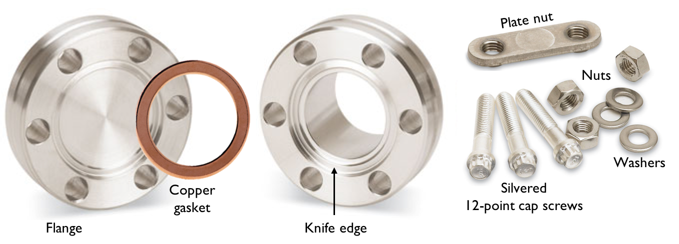
Figure B.4: Illustration of components needed for CF assembly. Figure modified from [441].

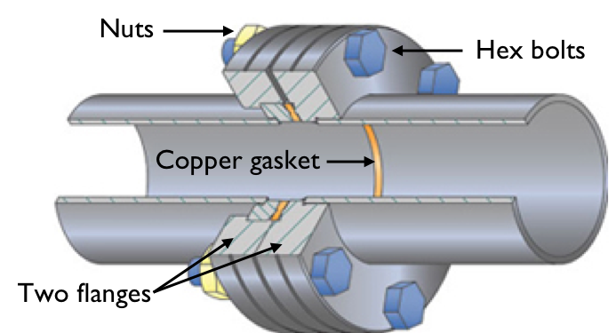
Figure B.5: Schematics of a CF seal. Figure from [441].

CF connections can be remade; however, a new gasket must be used for each new connection. If frequent reassemblies are expected, silver-plated 12-point cap screws are recommended. It is strongly recommended that all bolt, nuts, or plate nut combinations are lubricated to avoid thread galling, either by one component being silver-plated or by applying a suitable thread lubricant. For an assembly in a limited space, plate nuts can be used instead of individual nuts. These are metal plates with two threaded holes spaced apart so that they match the corresponding bolt holes. The plate nut act as its backing wrench so only one wrench is needed to tighten the bolts, which is desired if the other side of the flange cannot be accessed easily. Note that aluminum CF flanges must use either aluminum gaskets or elastomer gaskets. The use of elastomer gaskets is not appropriate for clean applications.

B.3 KF/ISO

The Klein Flansche (KF), also referred to as QF, connection permits rapid fitting and replacement of components in vacuum systems. The name KF was adopted by ISO, DIN, and other standards organizations. The connection is made with two symmetrical genderless flanges, a centering ring with an O-ring gasket, and a clamping ring as shown in Figure B.6. KF flanges are usually made from SS, aluminum, or brass. The properties of the O-ring limit the operating pressure and temperature ranges of the connection. The standards sizes are KF10, KF16, KF25, KF40, and KF50 where the number refers to the largest internal diameter (ID) (in mm) of a tube that can be welded to it.

To make the connection, a metal centering ring with an elastomeric O-ring around its OD is inserted between the two flanges. The centering ring fits into flanges’ counter-bore. A vacuum-tight connection is made without the use of tools by merely finger-tightening the circumferential clamping ring. Overtightening the clamp can deform the KF flange and can lead to galling of the screw-thread on the clamp if that style of clamp is used.

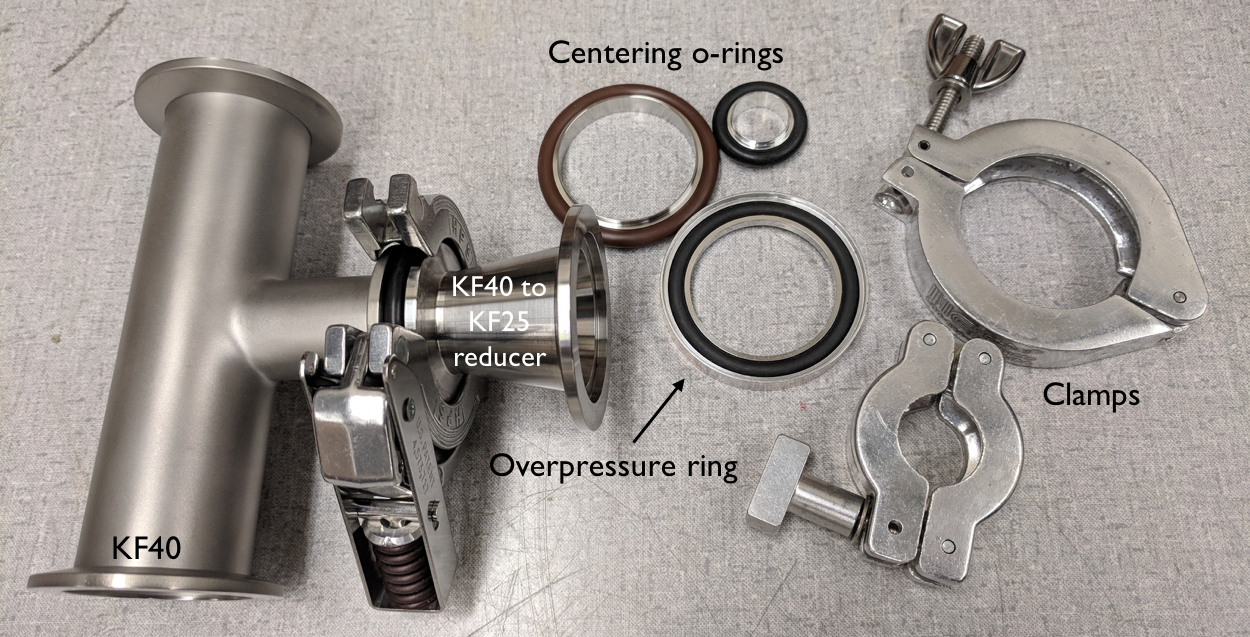
Figure B.6: Illustration of parts needed for a KF connection.

Metal overpressure rings can be installed around the O-rings if the system needs to operate at positive pressures. Depending on the KF diameter, this can increase the operating range up to 7 bar. Additionally, metal seals can be used instead of the standard elastomer O-rings. These metal seals require high contact pressures, but achieve a helium leak-tight seal and can be baked repeatedly up to 450^∘C depending on the O-ring material.

The design principles of ISO and KF seals are identical, but the ISO standard is used for tubing with a larger diameter. Because of this larger diameter, the ISO O-ring is more likely to roll off, so a spring-loaded retainer holds it externally. A variety of bolt and clamp options are used to mate ISO flanges.

B.4 Swagelok tube fittings

Swagelok tube fittings are a type of compression fittings available for all standard tubing diameters. The most appropriate use is in applications where the fitting will not be disturbed and will not be subjected to flexing or bending after assembly. Swagelok fittings can be used for both metal and plastic tubing. When used with metal tubing, Swagelok tube fitting forms an all-metal seal. Special non-metallic ferrules and tubing inserts have to be used with plastic tubing.

A significant advantage of Swagelok tube fittings is that it allows connection of two tubes without any welding or other work. However, once the joint is made, it cannot be disassembled and reassembled satisfactorily. The ferrules and part of the tube must be cut off, and a new ferrule should be used on a new piece of tubing. This assures a leak proof connection.

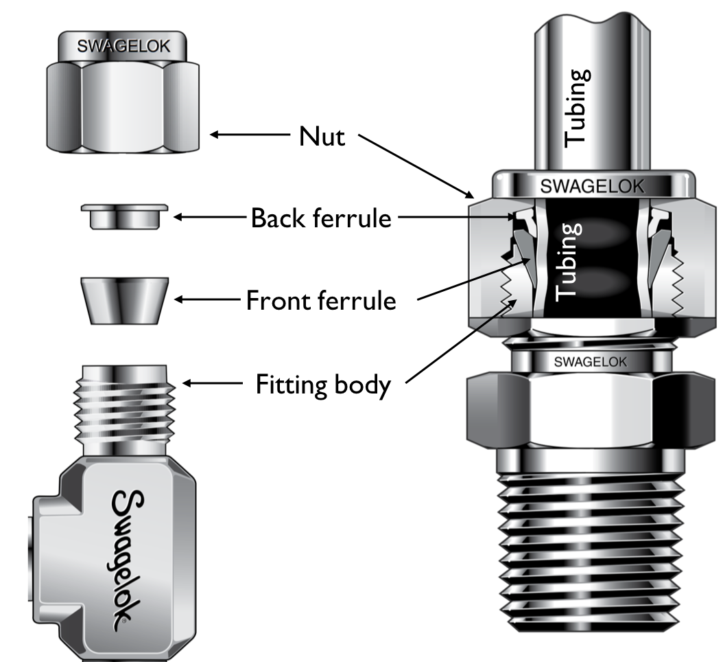
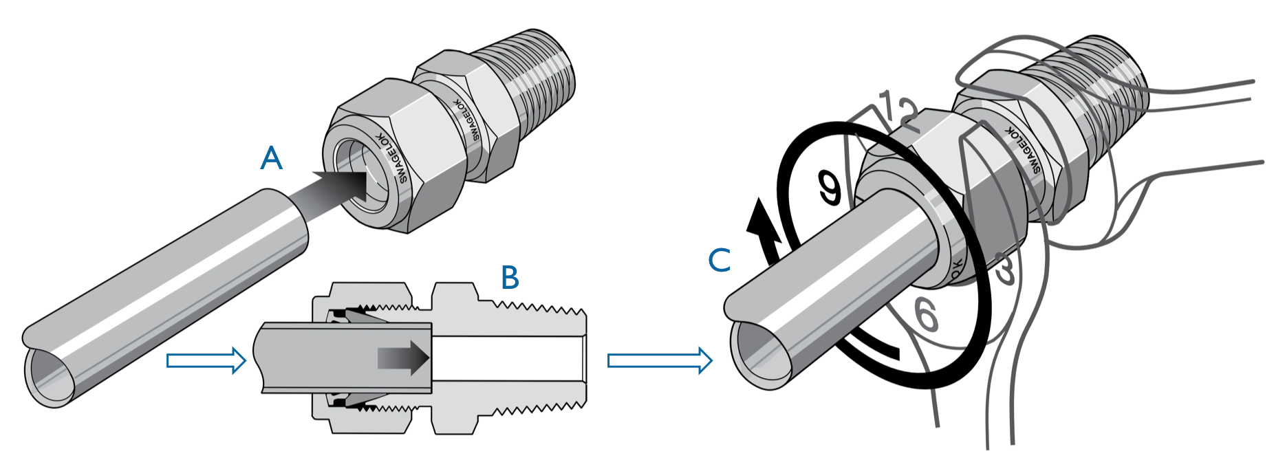
Figure B.7: Two-ferrule Swagelok tube fitting. The front ferrule creates a seal against the fitting body and to the outside diameter of the tubing. The back ferrule pushes the front ferrule forward and provides a grip on the tubing. Figure modified from [439].

Figure B.8: Illustration of steps to assemble Swagelok tube fitting. First, slip a female nut a piece of tubing (A), then press the tube against the ferrules inside the male part (B). Rotate the nut finger-tight and then tighten the connection using a pair of wrenches (C). Figure modified from [439].

To assemble fittings for tubes below 1 in OD, first, slip a female nut over a piece of tubing and press the tube against the ferrules inside the male part. Then rotate the nut finger-tight. For a reliable connection, tighten the nut until the tube will not turn by hand or slide out of the fitting, then mark the nut at the 6 o’clock position. Hold the male fitting body and tighten the female nut 1.25 additional turns to the 9 o’clock position as shown in Figure B.8. For tube fittings smaller than 3/16 in, tighten the connection by a pair of wrenches only by an additional 3/4 turn (to the 3 o’clock position). During the assembly, the front ferrule creates a primary seal against the fitting body and to the outside diameter of the tubing, which results in permanent deformation of the tubing as shown in Figure B.8. The back ferrule pushes the front ferrule forward and provides a grip on the tubing.

Swagelok does not recommend mixing components from various manufacturers, but the design is generically known as a compression fitting.

B.5 NPT

The National Pipe Tapered (NPT) thread is a standard used in the USA to join pipes and fittings. It is frequently used for pipes transporting liquids, gases, or steam. Unlike most other plumbing fittings that have straight or parallel threads, NPT fittings have a tapered thread profile illustrated in Figure B.9. The male thread has a larger OD at the base of the fitting that tapers down toward the opening, while the female part has the largest OD at the opening.

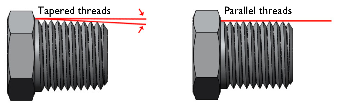
Figure B.9: Illustration of tapered (left) and parallel (right) threads. NPT uses tapered threads. Figure from [442].

Unlike all other fittings described in this appendix, NPT fittings seal at the threads as the male and female parts compress against each other. However, the threads may not align perfectly, which can leave a spiral leakage path. To mitigate that, NPT fittings are made leak free by applying a thread seal tape. Since the threads make the connection, the fittings should screw in only partway before jamming. If an NPT fitting bottoms out, the threads are either mis-tapped or worn out, and a new part should be used in assembly.

To make an NPT connection, clean the threads and apply a thread sealant, usually Teflon tape or thread, with the direction of the thread. Screw the parts together until finger-tight and then use a pair of wrenches to tighten the connection. Note that the nominal size of NPT fittings has minimal relation to the actual thread size; an NPT fitting measuring 3/8 in at the middle of the taper is actually an 1/8 in NPT. Therefore, a table should be referenced to identify the proper NPT fitting sizes.

Sometimes NPT threads are referred to as MPT (Male Pipe Thread), or MNPT for male threads, and FPT (Female Pipe Thread), or FNPT for female threads. There is also a variant called the National Pipe Thread Tapered Fine (NPTF), compatible with standard NPT fittings, designed to provide a better leak-tight seal without the use of Teflon tape (although Teflon tape can still be used). Note that British Standard Pipe (BSP) threads are used commonly outside the USA and are not compatible with NPT threads.

B.6 Flare fitting

Flare fittings are another type of compression fitting usually used with soft metal tubing. Flare fittings work well with natural gas and propane fuel lines, but can occasionally be encountered in the lab in high-pressure applications. The connection is straightforward to assemble and disassemble, but flare fittings require modification of the existing tube.

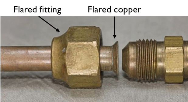
Figure B.10: Flare fitting. Figure from [443].

The fitting requires the tube to be formed in a flared taper at the end as shown in Figure B.10. The flared taper can be made using a special hand tool by cold working an even-cut end of a tube. The most common flare fitting standards in use today are the 45° SAE style, and the 37° AN style.

During the assembly, a female flared fitting nut is slipped over the tube and finger tightened to the male nut. Tightening the connection using a pair of wrenches produces a high-pressure, leak-tight seal. As usual, overtightening the nut should be avoided as it will cause the connection to lose its shape.

B.7 CGA 580

Compressed Gas Association (CGA) 580 is one of the many compressed gas cylinder outlet connections used in USA and Canada. Different standards are used in other parts of the world. Within the USA, slightly different standards are used for various gasses in various cylinders and are differentiated by a numeral; for example, CGA 540 is used for oxygen, while CGA 300 and 510 are used for acetylene. CGA 580 is used in particular for inert gasses such as helium, neon, argon, krypton, xenon, and nitrogen. Note that CGA connections can have either right- or left-hand threads depending on the contents of the cylinder.

A connection is made when a male nut presses the stem into the cylinder outlet as illustrated in Figure B.11. The connection should be tightened using a pair of wrenches.

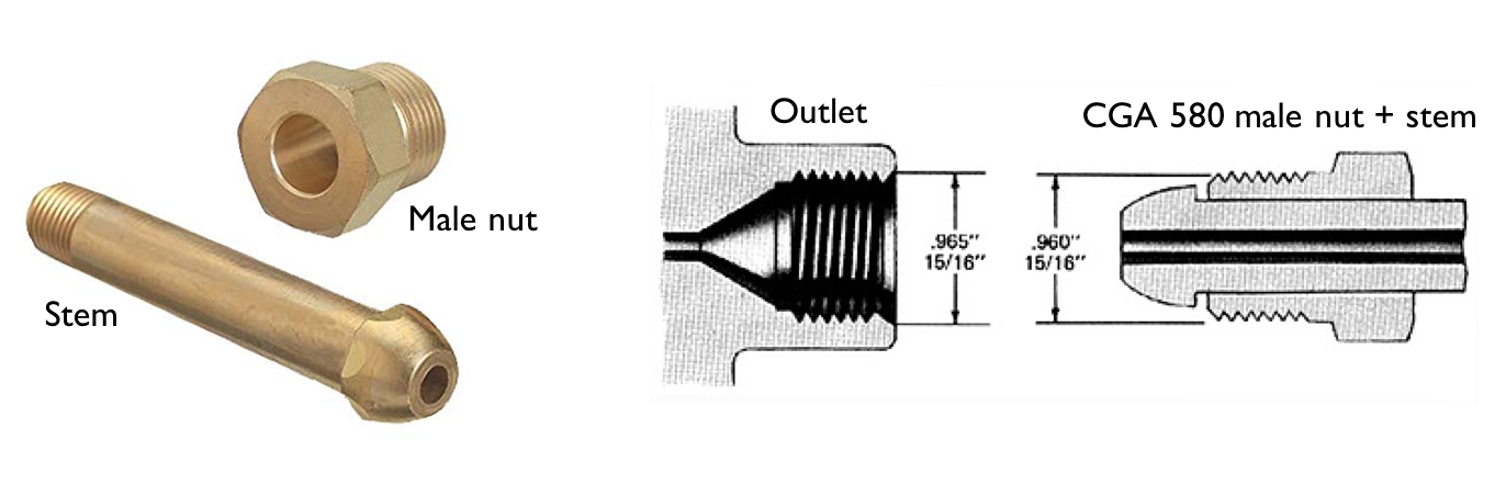
Figure B.11: Illustration of a CGA 580 connection. The male nut is free to rotate around the stem. When the stem is pressed into the outlet, it creates a seal. Figure modified from [444].

Appendix C XeBrA xenon condensing, circulation, and recovery procedure

This document outlines the procedure for condensation, circulation, and recovery of xenon in XeBrA. The detector is located at LBNL in room 70A-2263. The procedure assumes two bottles of xenon gas are attached to the gas system, and two recovery vessels in room 70A-2255 are connected to the gas system.

To begin a xenon fill, the gas system and detector are evacuated and prepared for cool down. A small amount of gas is introduced into the detector, and a constant pressure of gas is then maintained inside the detector while it is being cooled. Eventually, xenon starts condensing and fills the active volume. This process takes $\sim 18-48$ hours. Circulation should be started once the detector is full of liquid xenon to start removing impurities. Once a stable detector state is achieved, the detector is ready for data taking.

Since a stable detector state involves a constant stream of bubbles, it is necessary to slowly keep adding xenon during data taking to suppress bubbling as outlined below.

The P&ID can be found on the gas system panel and in Figure C.1.

Figure C.1: XeBrA’s gas system P&ID.

The following steps are performed during each cool down:

1. Leak checking

2. System evacuation

3. Introduction of xenon gas to the detector

4. Detector cool down and xenon condensation

5. Xenon circulation

6. Data taking

7. Xenon recovery

This document borrows from several LUX Critical Procedures: the LUX Detector Cooling Procedure, the LUX Condensing Procedure, and the LUX Circulation Critical Procedure.

C.1 Leak checking

This section outlines the procedure for leak checking the detector’s inner volume, the gas system, and the recovery vessels. Before using any helium for leak checking, turn on a big fan to prevent helium pile up in the room.

Do not operate pump SP01 under vacuum. The pressure ratio on input/output should never be larger than 5 (measured in absolute, not gauge, pressure).

C.1.1 Gas system leak check

1. Ensure manual valves (MV) MV01 and MV03 are closed to disconnect storage bottles.

2. Open regulator (RG) RG01.

3. Close MV10, MV11, MV12 and purge lines MV14, MV16 and MV18 to isolate XeBrA.

4. Close MV13 (connection to the IBEX experiment).

5. Attach leak checker to port behind MV12.

6. Open MV02, MV04, MV05, MV06, MV07, MV08, MV09, MV15, MV17, and MV19 to open the main circulation path.

7. Open MV12.

8. Start pumping.

9. Ensure the getter heater is off. As the pump is spinning up, switch the state of pneumatic valves (PV) PV01, PV02, and PV03 a couple of times to release trapped air by using the “valve control” button on the front of the getter housing.

10. Perform leak checking.

11. While leak checking the getter, ensure to switch the states once to check all connections.

12. Close MV12.

13. Turn off and disconnect the leak checker.

C.1.2 Circulation pump purge

The circulation pump is shown in Figure C.2. If the pump has not been exposed to air since previous detector fill, this step can be skipped. Purging the pump with clean argon gas ensures that any potential trapped volumes will be cleaned.

1. Attach argon gas cylinder with at least 99.999% purity as storage bottle (SB) SB01.

2. To ensure the getter is in the bypass mode (PV02 open), switch the getter bypass mode off using the “valve control” button on the front of the getter housing.

3. Close MV07, MV10, MV11, MV12 and MV14, MV16 and MV18.

4. Open a circulation path by opening MV06, MV08, MV09.

5. Fill the gas system with argon up to 1 barg (anything above 0 barg works). Follow the procedure for opening and closing xenon fill path from the gas bottle (Section C.3.3.1).

6. Run circulation pump SP01 at 5 SLPM or less for a minute.

7. Turn off circulation scroll pump (SP) SP01.

8. Open MV12 and carefully vent argon down to $\sim 0.1$ barg.

9. Close MV12.

10. Attach vacuum pump to MV12.

11. Open MV12.

12. Using vacuum pump attached to MV12, pump out the argon. MV01, MV02, MV05, MV06, MV07, MV08, MV15, MV17, and MV19 should be open. MV04, MV10, MV11, MV12, MV13, MV14, MV16, and MV18 should be closed.

13. Close MV12.

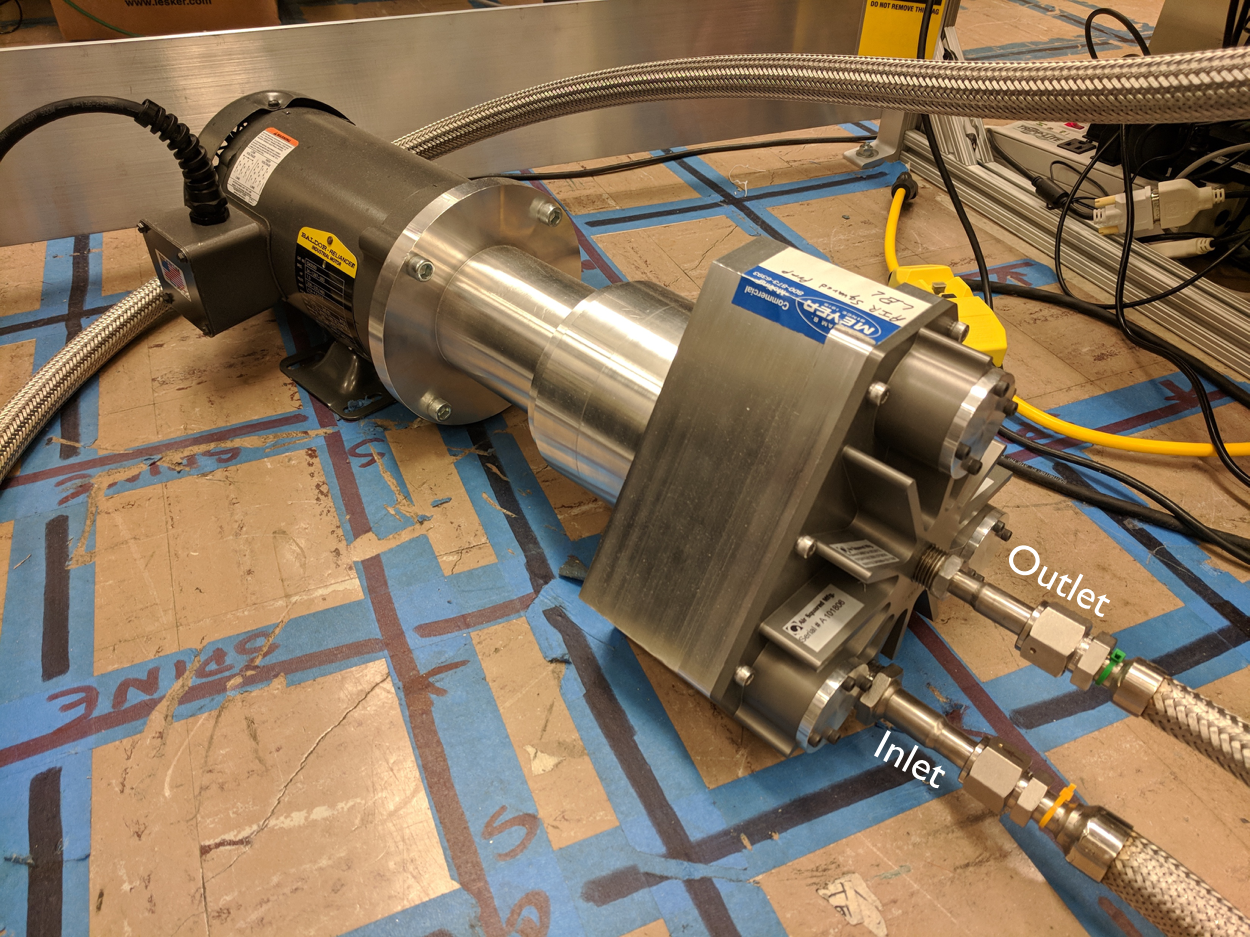
Figure C.2: Circulation pump.

C.1.3 XeBrA main volume leak check

1. Ensure MV10, MV11, and MV14, MV16, and MV18 are closed to isolate XeBrA.

2. Close the 6” gate valve (see Figure C.3 for location).

3. Make sure the turbo pump is off.

4. Attach the leak checker in place of the scroll pump backing XeBrA’s turbo pump (see Figure C.4).

5. Leak check.

6. Disconnect leak checker.

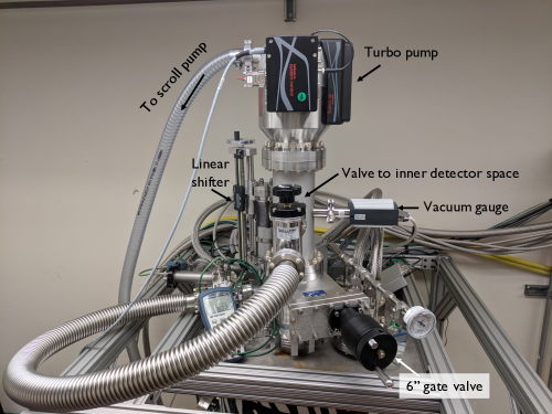
Figure C.3: Annotated photograph of the top of the XeBrA test stand.

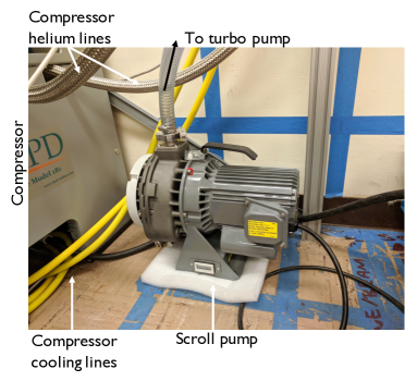
Figure C.4: XeBrA’s scroll pump and compressor.

C.1.4 Xenon recovery leak check

1. Ensure PV04 is closed.

2. Open MV20, MV21, and MV23.

3. Leak check each of the recovery vessels separately.

   1. To leak check SB03 (Rhino) connect a pump and a leak checker to MV22. Close MV23, open MV22 and perform the leak check. Close MV22 and disconnect the leak checker.

   2. To leak check SB04 (Hippo) attach a pump and a leak checker to MV24. Close MV23, open MV24 and perform the leak check. Close MV24 and disconnect the leak checker.

C.2 Evacuating XeBrA

This section outlines the procedure for evacuating the entire volume that will be filled with xenon. It is to be performed before every detector cool down.

1. Attach two xenon bottles as SB01 and SB02.

2. Ensure MV01 and MV03 are closed to isolate storage bottles.

3. Open MV02, MV04, MV05, MV06, MV07, MV08, MV09, MV10, MV11, MV14, MV15, MV16, MV17, MV18, and MV19. This opens the entire detector volume.

4. Open RG01 all the way.

5. Close and tag MV13 (connection to IBEX).

6. Close and tag MV12 (leak checking port).

7. Close the 6” gate valve (see Figure C.3 for location).

8. Open valve to inner space (see Figure C.3 for location).

9. Turn on XeBrA’s scroll pump and once the vacuum has reached 0.1 mbar turn on the turbo pump.

10. Pump out the entire detector and gas system volume for at least a day.

11. To pump out the getter, switch the getter bypass mode off using the “valve control” button on the front of the getter housing. Make sure the getter heater is off. After 10 minutes, enable the bypass mode again using the same button.

12. Pump until the vacuum pressure is lower than $1\times 10^{-6}$ mbar as read by the vacuum gauge near the turbo pump. Since the gauge is so close to the pump, the pressure in the rest of the volume will be higher, but sufficiently low.

13. Close the turbo pump’s access to inner space.

14. Turn off the turbo pump and let it spin down.

15. Once the turbo has spun down, start pumping on the outer vacuum vessel (OV).

16. Open the 6” gate valve and ensure that the valve to inner space (see Figure C.3 for locations) is closed.

17. Turn on the scroll pump, and once the vacuum has reach 0.1 mbar turn on the turbo pump.

18. Leave the scroll and the turbo pumping on the OV throughout xenon operations.

19. Separately, evacuate the two recovery vessels SB03 and SB04. Make sure that PV04 is closed. Attach a pump to MV22 and evacuate SB03 to least $1\times 10^{-2}$ mbar. Then attach a pump to MV24 and evacuate SB04 to the same pressure. If the vessels have been exposed to air between data runs, purge the vessels with argon gas prior to evacuating them to prevent contamination of potentially recovered xenon.

C.3 Introduction of xenon gas to the detector

This section introduces an initial amount of xenon gas to facilitate detector cooling. It assumes the detector has been leak checked and evacuated.

Exceeding 2.0 barg (29 psig) in the detector will result in the rupture of a burst disc (BD) BD07. If there is a severe problem during the condensing procedure follow the xenon recovery procedure in Section C.7.

C.3.1 Emergency precautions

This section describes precautions which must be in place whenever there is liquid xenon in the detector making overpressure possible.

1. Turn on to the Slow Control and verify it is functional.

2. Turn on email forwarding of alarms.

3. Set appropriate alarms as outlined in Section C.5.1.3.

   1. Ensure that high high alarms are at least 20% below the nearest burst disc value.

4. Appoint trained personnel with reliable communication devices to be on call within 1 hour of travel time while the detector contains any liquid xenon.

5. The Oxygen Deficiency Monitor (ODH) must be operational.

   1. There is a remote sensor in 70A-2263 and a local sensor inside the main control unit 70A-2255.

6. Ensure PV04 is closed and MV20, MV21, and MV23 are opened for a clear path to the recovery vessels.

   1. If needed, PV04 can be opened in Slow Control. It is password protected to avoid accidentally opening the valve.

      1. Password: XeBrA

C.3.1.1 SciNote logs

Make sure to log important milestones in SciNote, the electronic lab notebook [445]. Items to log include the amount of xenon left in SB01 & SB02, steady-state settings of the circulation pump (frequency setting and the resulting flow rate), and any other actions that differ from the regular procedures.

C.3.2 Gas system preparation

In this section, we ensure the gas system is in a known state, with appropriate valves locked to ensure that high pressure gas does not enter and break the hardware in the rest of the gas system.

1. Ensure MV01, MV02, MV03, and MV04 are closed to isolate the xenon storage bottles and prevent the introduction of xenon into the system before it is in the correct state.

2. To prevent high pressure from being accidentally introduced to the low pressure portion of the gas system, valve MV05 must be closed and tagged.

3. MV12 should be covered and tagged closed.

4. Close MV13 (connection to IBEX).

5. Ensure PV04 is closed and BD09 is intact (these open to the recovery line leading to 70A-2255).

6. Ensure MV20, MV21 and MV23 are opened to connect recovery vessels properly.

7. Ensure regulator RG01 is fully closed (i.e., in the zero-pressure position).

8. Ensure the Slow Control is properly activated and email forwarding of alarms is enabled.

9. Start slow data logging using the Slow Control (a 20 s save interval should be sufficient).

10. Ensure the outer vacuum volume is under vacuum maintained by the main turbo and scroll pumps as established at the end of the evacuating XeBrA procedure (Section C.2).

11. Ensure that recovery vessels SB03 and SB04 (Hippo and Rhino) have been evacuated to at least $1\times 10^{-2}$ mbar.

C.3.3 Initial xenon gas into detector

This procedure assumes the xenon volume has been evacuated. The fill is done using SB01. This is to be done while the detector is still warm.

Exceeding 2.0 barg (29 psig) in the detector will result in the rupture of a burst disc BD07.

1. Log the initial amount of gas in the bottle to SciNote by noting the weight of SC01.

2. Follow the gas system preparation procedure (Section C.3.2).

3. Close MV09, MV11, MV13, and MV14 through MV19.

4. Close and tag MV04 and MV12.

5. Open MV06, MV07, MV08, MV10.

6. Turn on the getter using the indicator LEDs and buttons on the getter front panel. The getter should be warm for 1 hour before gas introduction.

7. Make sure getter is not bypassed.

   1. The correct setting for a getter in operation is illustrated in Figure C.5.

8. Introduce xenon gas into the system by following the opening xenon fill path procedure (Section C.3.3.1).

9. Wait until the detector is full. This should only take a few minutes. Pressure indicator (PI) PI05 and pressure transducer (PT) PT05 should stabilize at the desired fill pressure of 0.5 barg.

10. Once the desired pressure is reached, follow the procedure for closing the xenon fill path (Section C.3.3.2) unless you are proceeding directly to the detector cooling (Section C.4).

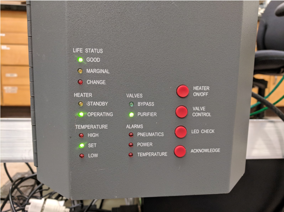
Figure C.5: Getter settings during operation. “Valves $\rightarrow$ Purifier” light should be green and “Heater $\rightarrow$ Operating” light should be blinking while the heater is on.

C.3.3.1 Opening the xenon filling path from the gas bottle

1. Ensure RG01 is fully closed (i.e., in the zero-pressure position).

2. Close and tag MV05.

3. Log the xenon mass in the bottle in SciNote.

4. Open MV01 and MV02.

5. This opens the path from the xenon gas storage bottle to the gas system panel.

6. Slowly open RG01 to let the desired amount of gas into the low pressure part of the gas system. Watch PI02/PT02 and PI05/PT05 for the desired pressure.

C.3.3.2 Closing the xenon filling path from the gas bottle

1. Log the xenon mass in the bottle in SciNote.

2. Close the bottle with MV01.

3. Slowly close RG01.

4. Close MV02.

   1. There might be pressure build up by PT01. This pressure will slowly leak into the detector through RG01 afterward and is expected. The pressure decrease over time indicated by PT01 does not (necessarily) mean there is a leak in that section of the gas system.

C.4 Detector cooling

Keep a close eye on temperatures all over the detector throughout this procedure. This section assumes the system is filled with 0.5 barg (7.3 psig) of xenon gas. Be sure to log important milestones in SciNote.

Monitor the cooling rate and pressure and ensure that the transfer gas in the detector does not freeze by maintaining the pressure above the triple point of xenon (0.8 bar - see Figure C.6). Exceeding 2.0 barg in the detector will result in the rupture of a burst disc BD07.

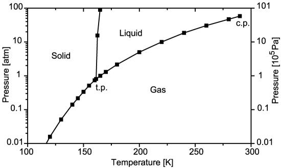
Figure C.6: Phase diagram of xenon. Triple point (t.p.): 161.3 K, 81.6 kPa. Critical point (c.p.): 289.7 K, 5.88 MPa. Unit conversions: 1 atm = 101,325 Pa; 0 C = 273.15 K. Figure from [446].

C.4.1 Starting the pulse tube refrigerator

It is not advised to fill a detector that does not have a functioning heater. Check both heaters attached at the bottom of the detector by turning them on briefly in the Slow Control and seeing the temperature on RTD3 and RTD4 rise.

1. Ensure that acceptable vacuum in the OV has been achieved ($1\times 10^{-4}$ mbar for cooling, and $1\times 10^{-5}$ or better for HV operations).

   1. This can be read off from the “System vacuum” in the Slow Control.

2. Make sure helium lines are between the Pulse Tube Refrigerator (PTR) and the compressor. Make sure that cooling lines are plugged to the compressor and the water supply and return.

3. Ensure helium pressure in compressor is at $200\pm 5$ psig by checking the gauge on the front of the compressor. If the pressure is lower/higher top up/relieve helium. Procedure for this is included in the compressor manual.

4. Turn the water supply and return fully on.

5. Plug in the compressor into the mains.

6. Turn on the compressor.

C.4.2 Xenon condensing

1. Follow the procedure for opening the xenon fill path from the bottle (Section C.3.3.1).

2. Set RG01 to 0.5 barg.

   1. To check the settings of the regulator, ensure that MV11, MV14, MV16, and MV18 are closed.

   2. Temporarily close MV06. Carefully monitor PT03, PT04, and PT05 to not over-pressurized the detector.

   3. Open RG01 to the desired pressure by observing PT02.

   4. Reopen MV06.

3. Monitor the temperature of the heat exchanger. For a given pressure in the detector, use the vapor curve to calculate the condensation temperature. The rate of cooling of the detector will increase once an initial amount of xenon has condensed.

4. The thermometers on the PTR and heat exchanger will be the first to register cooling. These are:

   1. RTD1 & RTD2 on heat exchanger

   2. RTD6 on the PTR.

   3. The rest of the RTDs will follow over time.

5. Expect a total cooling time of the metal bulk of several hours (see Section C.8 for details).

6. The condensation phase begins once enough of the detector reaches the vapor curve.

   1. Find the condensation temperature from the vapor curve of xenon in Figure C.7 (-101 C at 0.5 barg).

7. It is important to keep the pressure well above 0.8 bar (see Figure C.6) at the beginning of the condensation phase to prevent freezing. The open regulator RG01 should prevent this.

8. Every few hours, determine the amount of gas condensed in the detector and log it in SciNote. Based on this calculation one can extrapolate expected fill time.

   1. Use the scale SC01 to determine the amount of xenon that has already condensed in the detector.

   2. Once the detector is nearly full, liquid level should be visible through the detector window.

9. Assuming the condensation proceeds as expected one should see the level sensor changing value. When the capacitance value has stopped increasing, condense an additional 0.5 l of xenon, then proceed to start circulation. This guarantees that the liquid exit is submerged.

10. Close xenon filling path from the gas bottle (Section C.3.3.2).

Figure C.7: Xenon vapor curve. Figure from [447].

C.5 Circulation start

At this point, the detector is filled with liquid, and the evaporator should be at a similar temperature to the condenser. The purge lines should be opened when using the PMT or the purity monitor.

Monitor the detector pressure (PT05) and ensure it does not drop below 0.8 bar by adjusting the heater in the Slow Control. Exceeding 2.0 barg (29 psig) in the detector will result in the rupture of a burst disc BD07.

1. Close MV01, MV02, RG01, MV09, and MV14 through MV19.

2. Open purge valves MV14, MV16, and MV18.

3. Open MV06, MV08, MV10, and MV11.

4. Close the pump bypass valve MV07.

5. Start the pump by slowly increasing the pump speed by 1 Hz until FM01 reads 2 SLPM.

6. Note the pressure difference between PT03 and PT04. The pressure difference at the pump outlet (PT04) should not be more than 5 times as large as the pressure at the pump inlet (PT03).

   1. Note: Running the circulation pump fast will add a heat burden.

7. Slowly increase the pump speed and observe the pressures and temperatures throughout the circulation path. If the circulation is going too fast, a stream of bubbles will be visible in the detector at the location of xenon inlet. This means that xenon is not being liquefied inside the heat exchanger. If the pump is going too slow, the pressure might continue to decrease and cause the detector to start freezing xenon because not enough heat is being introduced into the system. If you can circulate faster than $\sim 5$ SLPM while maintaining stable pressure, you have established an efficient heat exchange.

   1. The settings are likely to differ slightly for each cool down, based on the amount of xenon condensed to the detector. In 2018 stable circulation was achieved with the pump at $8-10\,\mathrm{Hz}$, circulation speeds of $\sim 20\,\mathrm{SLPM}$, and the PTR heater at 100% while circulating through the getter.

8. Set up the PTR heater on its seesaw setting and circulate happily ever after.

   1. If the detector pressure keeps dropping, the bottom heaters can be turned on to help raise detector pressure.

   2. It usually takes 12-24 hours for the detector to settle into a stable state. Many adjustments may be necessary in the interim.

9. Once the detector appears stable, adjust the circulation to the desired flow rate.

   1. Note: Faster circulation speeds achieve less efficient thermal exchange in the heat exchanger.

   2. Note: The recommended circulation speed by the getter to achieve efficient removal of impurities is 15 SLPM. However, the getter’s internal temperature has been increased since xenon has a lower thermal conductivity so optimal purifying speeds are likely around (or slightly below) this value.

10. Set alarms as outlined in Section C.5.1.3.

11. To collect HV breakdown data follow Section C.6.

C.5.1 Slow control settings

C.5.1.1 Settings for stable circulations

• Pump between 6-10 Hz (the flow rate on FM01 should be 20-25 SLPM).

• PTR Heater cycle is on with pressure boundaries on PT05 set with 0.01 bar pressure difference.

C.5.1.2 LabView interruption

If LabView is stopped during detector operations (which can happen if Windows forces a restart to install updates), the pump and getter will also shut off, but otherwise stopping LabView alone should not change detector operations. Turning off the PLC is strongly discouraged during detector operations.

After LabView code is restarted ensure that:

1. The getter is not bypassed.

   1. The correct setting for a getter in operation is illustrated in Figure C.5.

2. The pump and PTR heater cycle are on correct settings and operational.

3. Turn slow data logging back on and ensure email alarm forwarding is on.

4. Check back in a few hours to make sure the detector is in a stable state.

C.5.1.3 Alarm settings during circulation

This list of alarms assumes that the detector is operating at 1.0 barg. The alarms should be modified during condensation or recovery as needed. Low and high alarms only trigger an email notification. Low low and high high pressure alarms trigger email notification and interlocks. In general, for setting high alarms, the user should find the nearest burst disc to inform the threshold selection. High high alarms should be at least $20\%$ below the nearest burst disc rating to avoid a rupture.

	PT01 [barg]	PT02 [barg]	PT03 [barg]	PT04 [barg]	PT05 [barg]	PT07 [psi]
Low low	N/A	0.1	0.1	0.1	0.1	N/A
Low	0.1	0.7	0.3	0.7	0.7	200
High	10.0	1.3	1.3	3.0	1.3	N/A
High high	N/A	1.8	1.8	5.0	1.8	N/A

	FM01 [SLPM]	System vacuum [mbar]	HV vacuum [mbar]
Low	0	N/A	N/A
High	30	$1\times 10^{-4}$	$1\times 10^{-5}$

Table C.1: Alarm settings for detector operations while circulating. PT03 is at the pump inlet, so it reaches lower pressures than the rest of the system. Similarly, PT04 is at the pressure outlet and can reach higher pressures than the rest of the system. PT07 is installed on the compressed nitrogen cylinder used for pneumatic valve actuation. The low alarm notifies the user to purchase and install a new cylinder. FM01 is rated to 50 SLPM. Since the thermal coupling of the RTDs to the system is not optimal, the temperature set points need to be adjusted after each fill.

C.6 Data taking

Once the detector is stable (usually about one day after completing the fill), one can start taking HV data. This requires suppressing bubbles, which can be achieved by adding xenon into the detector. Assume that target detector pressure for data taking is 1.0 barg.

Monitor the detector temperatures to avoid excessive xenon ice formation in the detector.

1. Prior to data taking, keep the detector $\sim 0.3$ barg below target pressure for $\sim 12$ hours.

2. Slow down the circulation slightly.

3. With the detector circulating, ensure RG01 is closed.

4. Open MV01 and MV02 to open path of xenon to the detector.

5. Slowly open RG01. The pressure will rise fast at first until the target pressure of 1.0 barg is reached.

   1. Monitor temperature in the detector throughout data taking. If the temperature of the PTR and the heat exchanger start dropping dramatically, ice has started forming in the heat exchanger. Stop data taking and carefully begin warming the heat exchanger using the attached heater.

   2. If a small amount of ice starts forming at the bottom of the cone, but not in the heat exchanger, this is okay. This might enable stable data taking without the need to add xenon.

6. This creates a stable, bubble-free detector for HV data taking.

To start taking HV data:

1. Zero electrodes and note the distance on the caliper.

2. Set electrodes to the desired separation.

3. Ensure the PMT is off.

4. Turn off purity monitor’s charge amp and ensure surge protector is grounded.

5. Disconnect the capacitor by unplugging the banana plugs.

6. Ensure the top electrode is grounded.

   1. Either plug a shorted cable to the signal SHV channel,

   2. or plug in the charge sensing box.

7. Start fast data logging in Slow Control.

Ensure the detector is bubble free throughout the data taking and that the spark is occurring between the two electrodes.

C.7 Xenon recovery

This procedure empties all xenon from the entire system. First, the recovery vessels are cooled down to below xenon freezing point, with heaters on the storage bottle’s valve to prevent valve damage. Then, the gas system is prepared for recovery before pulling all the xenon from XeBrA into one of the aluminum storage cylinders.

Ensure that the ODH monitor in the room is working and wear a portable ODH monitor. Expect to take a full day to recover the entire detector volume ($\sim 10$ hours). Never walk away from the detector until you are certain all the xenon is in the storage bottle and that bottle is closed.

Note the start and end of detector warm up in SciNote. Always have nitrogen in the transfer dewar throughout this procedure. A single 160 l transfer dewar should be sufficient for one recovery.

1. Slowly turn off the pump SP01 by stepping down the frequency 1 Hz at the time..

2. Turn off the getter and set to bypass using the buttons on the front of the getter housing.

3. Monitor oxygen levels during the liquid nitrogen (LN) fill and turn on the big fan to encourage air circulation.

4. Figure out which bottle you want to use for recovery (SB01 or SB02) and make sure it contains either vacuum or xenon. This procedure assumes recovery into SB01. Fill the dewar that contains your bottle of choice with LN about half way and wait for the temperature to equalize. This will take 0.5-1 hour depending on the quantity of xenon left in the aluminum bottle.

   1. MV01 contains elastomer seals so it is important to find the Goldilocks equilibrium. To prevent valve damage a heater or a heating tape should be installed on the top of SB01 and around MV01. It is also important to not overheat the valve.

   2. Once you are sure that SB01 is cold enough (nitrogen is no longer violently boiling) you can start recovery.

5. Open MV06, MV07, MV08, MV09, MV10, MV11, and MV14 through MV 19.

6. Close RG01, MV03, and MV04.

7. Open MV01 and MV02. This will open up the path to SB01.

8. Check PT01 to verify that SB01 is at negligible pressure before opening MV05.

9. Open MV05. This opens the path from detector to SB01 and xenon should start freezing in the bottle.

10. Set up high alarms for the bottom cone heaters in Slow Control.

11. Turn on the heater at the bottom of the cone. Monitor the thermometers and ensure the detector does not get too hot once the xenon has evaporated - the alarms should trigger an interlock turning off the heaters once the threshold is exceeded.

12. Ensure the pressure does not go below 0.1 barg during recovery to prevent xenon contamination.

13. Once you are sure the pressure is falling steadily, turn off PTR and its water cooling.

14. After a while, you can turn off the turbo and later also the scroll pump to increase the heat load on the detector.

    1. If you want to increase the heat load, introduce a small amount of nitrogen gas into the OV. Avoid exposing this volume to air since that would cause water condensation on surfaces.

15. Keep topping up the dewar with liquid nitrogen until you are confident that all the xenon has been recovered into SB01.

16. Close MV01. Do not close MV01 if it is too hot (too hot to touch) or too cold (frosted) to prevent damaging the valve.

17. Once all liquid nitrogen has evaporated, log the final weight of SB01 in SciNote.

C.7.1 Emergency recovery

If the detector pressure exceeds the pressure set by an alarm on PT05, emergency xenon recovery will trigger. In this case, PV04 will open automatically, thus allowing xenon to enter vessels SB03 (Rhino) and SB04 (Hippo). PV04 will stay open while the pressure is above the defined threshold. Once the pressure falls below the alarmed threshold, PV04 will close automatically.

If there is xenon in SB03 and SB04, it then needs to be recovered via cryopumping at the end of a run. To do that, once step 16 in Section C.7 is achieved (all the xenon from the main detector volume has been recovered):

1. Close off the detector volume by closing MV10, MV11, MV14, MV16, and MV16.

2. Open PV04.

   1. PV04 can be opened in Slow Control. Password: XeBrA

3. Wait until all the xenon has been recovered. Then proceed to Step 17 in Section C.7.

C.8 Calculations

The calculations below serve only to find back-of-the-envelope numbers so should be treated appropriately.

C.8.1 Heat needed to cool down detector

Assume all stainless steel and the room-temp specific heat is constant to the liquid xenon temp. This calculation does not assume the presence of xenon gas in the detector, which is expected to improve the thermal conductivity, so the time calculated here is an upper limit.

• XeBrA’s mass is $\sim 50$ kg

• Thermal conductivity decreases with temperature; the following calculation uses specific heat of stainless steel at room temp of $c_{V}=490\,\mathrm{J/kg\cdot K}$

• Temperatures: $T_{room}=293\,\mathrm{K}$ , $T_{LXe}=165\,\mathrm{K}$

Heat $Q$ needed to cool down the detector to 165 K assuming it is made entirely of stainless steel

$$Q=c_{V}\cdot m\cdot dT=3.1\,\mathrm{MJ}.$$ (C.1)

The cooling power $P$ of PTR is 40 W at 80 K. Therefore, the time needed to cool down the detector

$$T=\frac{Q}{P}=22\,\mathrm{hours}.$$ (C.2)

C.8.2 Estimated time to condense xenon

This calculation considers the xenon gas introduced to the detector and estimates the heat needed first to cool it to the vapor curve and then condense it.

• Volume $V_{LXe}=5.6\,\mathrm{l}$

• Density at 3 bar $\rho_{LXe}=2.94\,\mathrm{kg/l}$, resulting in mass $m_{LXe}=16.5\,\mathrm{kg}$

• Specific heat $c_{V_{LXe}}=97\,\mathrm{J/kg\cdot K}$

• Latent heat $L_{LXe}=12.64\,\mathrm{kJ/mol}$

• Molar mass of LXe is 131.3 g/mol

The heat needed to cool gaseous xenon down to 165 K is

$$Q=c_{V}\cdot m\cdot dT=205\,\mathrm{kJ}.$$ (C.3)

The latent heat of vaporization for LXe is

$$Q=m\cdot L=1588\,\mathrm{kJ}.$$ (C.4)

Therefore, the total heat needed is 1793 kJ, which results in a time needed to cool and condense the xenon of 12.3 hours.

C.8.3 Power radiated from XeBrA

While the detector is filled with liquid xenon, it will absorb and emit light (heat) from the environment. The power absorbed by the detector is

$$P =A\sigma\epsilon\left(T^{4}-T_{0}^{4}\right)$$

$$=86.2\,\mathrm{W}$$

where the Stefan-Boltzmann constant, $\sigma=5.67\times 10^{-8}\,\mathrm{W/\left(m^{2}\cdot K^{4}\right)}$, describes the power radiated from a black body in terms of its temperature, $A=1.6\,\mathrm{m^{2}}$ is the area of the active detector volume, and the emissivity $\epsilon$ of polished 304 stainless steel at 87 K is 0.13. The temperature $T=293\,\mathrm{K}$ corresponds to the radiation absorbed while $T_{0}=165\,\mathrm{K}$ corresponds to the radiation emitted.

To improve the cooling power available to the detector, the power radiated by the detector can be decreased if the active volume is wrapped in several layers of superinsulation. This helps to reduce the heat absorbed by the detector because the outgoing radiation is much weaker compared to the incoming radiation. Reference [448] says that under a good vacuum, a typical value of the heat transfer for a non-compressed 20-layer multi-layer insulation system is $\sim 1-3\,\mathrm{W/m^{2}}$ from $80-300$ K and $<100\,\mathrm{mW/m^{2}}$ between $4-80$ K. XeBrA was wrapped in $\sim 20$ layers of superinsulation so we can expect a reduction of the radiated heat by a few watts.

Appendix D XeBrA parts list

This appendix lists selected parts used in the gas system and XeBrA as described in Chapter 6.

Part	Manufacturer	Model
Spherical square vacuum chamber	Kimball physics	MCF600-SphSq-F2E4A8
Linear shifter	Kurt J. Lesker	LSM38-200-H-DL
HV power supply	Spellman	SL100N10/CMS/LL20
HV cable	Dielectric Sciences	2121
Vacuum-xenon feedthrough	CeramTec	6722-01-CF
Air-vacuum feedthrough	Isolation Products	D-102-10
Pulse tube refrigerator	Cryomech	PT805
Compressor	Cryomech	CP950
Current monitor	Pearson electronics	110A
Picoammeter	Keithley	6487
Capacitance meter	BK Precision	890C
Vacuum gauges	Leybold	Ionivac ITR 90
Pressure relief valve	Accu-Glass	113160
Power supply for purity monitor	Stanford Research Systems	PS350
Oscilloscope	Tektronix	TDS5034B
Xenon flash lamp	Hamamatsu	L9455-11
Argon PMT	Hamamatsu	R8520-06
Xenon PMT	Hamamatsu	R9228
Pressure recording film (2-20 psi)	McMaster Carr	3145K22

Table D.1: List of selected parts used in XeBrA.

P&ID label	Part	Manufacturer	Model
SP01	Scroll circulation pump	Air Squared	P15H22N4.25
FT01	Filter	Swagelok	SS-SCF3-VR4-P-225
CZ01	Check valve	Swagelok	SS-4CA-VCR-50
RG01	Regulator	APTech	AP1202S-2PW-FV4-FV4
FR01-03	Flow restrictor	Mott Corp	5140-1/4-SS-50
FM01	Flow meter	Aalborg	GFM37S-VCL6-A0
PV04	Pneumatic valve	Swagelok	6LVV-DPFR4-P-C
MV02, MV04-05	Manual high pressure valve	Swagelok	6LVV-DPHFR4-P
MV06-08, MV10-20	Manual valve	Swagelok	6LVV-DPFR4-P
PI02-03, PI05-06	Pressure gauge	Swagelok	PGU-50-PC60-C-4FSF
PT02-03, PT05-06	Pressure transducer	GE	PTX5072-TA-A1-CA-H0-RA
BD07-08	Burst disc	Continental Disc	CD30669A0126
SC01, SC02	Scale	Adam	CPWplus 200M
SB01, SB02	Aluminum cylinder	Evergreen	I-265-580
SB03, SB04	Xenon recovery vessel (i.e., a propane tank)	Manchester Tank	1499TC.11HL
	Open top nitrogen dewar	Cryofab	CF1636
	Vacuum gauges	Pfeiffer Vacuum	TPG361
	Getter	SAES Pure Gas	PF4-C15-R-1
	High current GFCI for getter	North Shore Safety	PGFI-1311N-138
	PUR-Gas™ In-Line Purifiers	Matheson Tri-Gas	SEQPURILOMT1
	Permanent oxygen monitor	Alpha Omega	Series 1300

Table D.2: List of parts used in the gas system. The P&ID is shown in Figure 6.17. If various models of the part are used for different pressure conditions, only one of the models is listed in the table. GFCI stands for Ground Fault Current Interrupter.

References

- [1] F. Zwicky, Republication of: The redshift of extragalactic nebulae, General Relativity and Gravitation 41 (Jan, 2009) 207–224.
- [2] T. Baker, D. Psaltis and C. Skordis, Linking tests of gravity on all scales: from the strong-field regime to cosmology, The Astrophysical Journal 802 (2015) 63, [http://stacks.iop.org/0004-637X/802/i=1/a=63].
- [3] E. Bellini, A. J. Cuesta, R. Jimenez and L. Verde, Constraints on deviations from CDM within Horndeski gravity, JCAP 1602 (2016) 053, [1509.07816].
- [4] A. G. Riess et al., Observational evidence from supernovae for an accelerating universe and a cosmological constant, The Astronomical Journal 116 (1998) 1009, [http://stacks.iop.org/1538-3881/116/i=3/a=1009].
- [5] S. Perlmutter et al., Measurements of and from 42 high-redshift supernovae, The Astrophysical Journal 517 (1999) 565, [http://stacks.iop.org/0004-637X/517/i=2/a=565].
- [6] M. Tegmark et al., Cosmological constraints from the SDSS luminous red galaxies, Phys. Rev. D 74 (Dec, 2006) 123507.
- [7] B. Ryden, Introduction to cosmology. Cambridge University Press, 2003.
- [8] F. Iocco, G. Mangano, G. Miele, O. Pisanti and P. D. Serpico, Primordial nucleosynthesis: From precision cosmology to fundamental physics, Physics Reports 472 (2009) 1 – 76.
- [9] S. Sarkar, Big Bang nucleosynthesis and physics beyond the standard model, Rept. Prog. Phys. 59 (1996) 1493–1610, [hep-ph/9602260].
- [10] A. Del Popolo, Nonbaryonic Dark Matter in Cosmology, Int. J. Mod. Phys. D23 (2014) 1430005, [1305.0456].
- [11] G. D’Amico, M. Kamionkowski and K. Sigurdson, Dark Matter Astrophysics. Springer Netherlands, Dordrecht, 2011.
- [12] J. C. Mather and other, A preliminary measurement of the cosmic microwave background spectrum by the Cosmic Background Explorer (COBE) satellite, The Astrophysical Journal 354 (1990) L37–L40.
- [13] COBE collaboration, G. F. Smoot et al., Structure in the COBE differential microwave radiometer first year maps, Astrophys. J. 396 (1992) L1–L5.
- [14] Planck collaboration, R. Adam et al., Planck 2015 results. I. Overview of products and scientific results, Astron. Astrophys. 594 (2016) A1, [1502.01582].
- [15] W. Hu, Lecture Notes on CMB Theory: From Nucleosynthesis to Recombination, 0802.3688.
- [16] Planck collaboration, N. Aghanim et al., Planck 2018 results. VI. Cosmological parameters, 1807.06209.
- [17] W. Hu and S. Dodelson, Cosmic microwave background anisotropies, Ann. Rev. Astron. Astrophys. 40 (2002) 171–216, [astro-ph/0110414].
- [18] D. J. Eisenstein, H.-j. Seo and M. J. White, On the Robustness of the Acoustic Scale in the Low-Redshift Clustering of Matter, Astrophys. J. 664 (2007) 660–674, [astro-ph/0604361].
- [19] SDSS collaboration, D. J. Eisenstein et al., Detection of the Baryon Acoustic Peak in the Large-Scale Correlation Function of SDSS Luminous Red Galaxies, Astrophys. J. 633 (2005) 560–574, [astro-ph/0501171].
- [20] SDSS collaboration, D. G. York et al., The Sloan Digital Sky Survey: Technical Summary, Astron. J. 120 (2000) 1579–1587, [astro-ph/0006396].
- [21] C. Patrignani and P. D. Group, Review of particle physics, Chinese Physics C 40 (2016) 100001, [http://stacks.iop.org/1674-1137/40/i=10/a=100001].
- [22] M. Kowalski et al., Improved cosmological constraints from new, old, and combined supernova data sets, The Astrophysical Journal 686 (2008) 749, [http://stacks.iop.org/0004-637X/686/i=2/a=749].
- [23] A. M. Boesgaard and G. Steigman, Big Bang Nucleosynthesis: Theories and Observations, Annual Review of Astronomy and Astrophysics 23 (1985) 319–378, [https://doi.org/10.1146/annurev.aa.23.090185.001535].
- [24] D. N. Schramm and M. S. Turner, Big-Bang nucleosynthesis enters the precision era, Rev. Mod. Phys. 70 (Jan, 1998) 303–318.
- [25] C. Afonso et al., Limits on Galactic dark matter with 5 years of EROS SMC data, A&A 400 (2003) 951–956.
- [26] C. Alcock et al., The MACHO Project: Microlensing Results from 5.7 Years of Large Magellanic Cloud Observations, The Astrophysical Journal 542 (2000) 281, [http://stacks.iop.org/0004-637X/542/i=1/a=281].
- [27] G. Steigman, Primordial nucleosynthesis in the precision cosmology era, Annual Review of Nuclear and Particle Science 57 (2007) 463–491, [https://doi.org/10.1146/annurev.nucl.56.080805.140437].
- [28] D. Clowe, M. Bradac, A. H. Gonzalez, M. Markevitch, S. W. Randall, C. Jones et al., A direct empirical proof of the existence of dark matter, Astrophys. J. 648 (2006) L109–L113, [astro-ph/0608407].
- [29] D. Harvey, R. Massey, T. Kitching, A. Taylor and E. Tittley, The non-gravitational interactions of dark matter in colliding galaxy clusters, Science 347 (2015) 1462–1465, [1503.07675].
- [30] Y. Sofue and V. Rubin, Rotation curves of spiral galaxies, Ann. Rev. Astron. Astrophys. 39 (2001) 137–174, [astro-ph/0010594].
- [31] V. C. Rubin, N. Thonnard and W. K. Ford, Jr., Rotational properties of 21 SC galaxies with a large range of luminosities and radii, Astrophys. J. 238 (1980) 471.
- [32] J. F. Navarro, C. S. Frenk and S. D. M. White, The Structure of cold dark matter halos, Astrophys. J. 462 (1996) 563–575, [astro-ph/9508025].
- [33] J. L. Feng, Dark matter candidates from particle physics and methods of detection, Annual Review of Astronomy and Astrophysics 48 (2010) 495–545, [https://doi.org/10.1146/annurev-astro-082708-101659].
- [34] J. M. Cline, TASI Lectures on Early Universe Cosmology: Inflation, Baryogenesis and Dark Matter, 1807.08749.
- [35] P. Cushman et al., Working Group Report: WIMP Dark Matter Direct Detection, in Proceedings, 2013 Community Summer Study on the Future of U.S. Particle Physics: Snowmass on the Mississippi (CSS2013): Minneapolis, MN, USA, July 29-August 6, 2013, 2013. 1310.8327.
- [36] R. D. Peccei and H. R. Quinn, CP Conservation in the Presence of Pseudoparticles, Phys. Rev. Lett. 38 (1977) 1440–1443.
- [37] S. Weinberg, A new light boson?, Phys. Rev. Lett. 40 (Jan, 1978) 223–226.
- [38] F. Wilczek, Problem of Strong P and T Invariance in the Presence of Instantons, Phys. Rev. Lett. 40 (Jan, 1978) 279–282.
- [39] G. G. Raffelt, Astrophysical axion bounds, Lect. Notes Phys. 741 (2006) 51–71, [hep-ph/0611350].
- [40] P. Sikivie, Experimental Tests of the Invisible Axion, Phys. Rev. Lett. 51 (1983) 1415–1417.
- [41] ADMX collaboration, C. Boutan et al., Piezoelectrically Tuned Multimode Cavity Search for Axion Dark Matter, Phys. Rev. Lett. 121 (2018) 261302, [1901.00920].
- [42] HAYSTAC collaboration, L. Zhong et al., Results from phase 1 of the HAYSTAC microwave cavity axion experiment, Phys. Rev. D97 (2018) 092001, [1803.03690].
- [43] CAST collaboration, V. Anastassopoulos et al., New CAST limit on the axion-photon interaction, Nature Physics 13 (05, 2017) 584–590.
- [44] S. J. Asztalos, L. J. Rosenberg, K. van Bibber, P. Sikivie and K. Zioutas, Searches for astrophysical and cosmological axions, Ann. Rev. Nucl. Part. Sci. 56 (2006) 293–326.
- [45] B. M. Brubaker, First results from the HAYSTAC axion search. PhD thesis, Yale University, 2018.
- [46] M. A. Shifman, A. I. Vainshtein and V. I. Zakharov, Can Confinement Ensure Natural CP Invariance of Strong Interactions?, Nucl. Phys. B166 (1980) 493–506.
- [47] M. Dine, W. Fischler and M. Srednicki, A simple solution to the strong CP problem with a harmless axion, Physics Letters B 104 (1981) 199 – 202.
- [48] OSQAR collaboration, R. Ballou et al., New exclusion limits on scalar and pseudoscalar axionlike particles from light shining through a wall, Phys. Rev. D92 (2015) 092002, [1506.08082].
- [49] PVLAS collaboration, E. Zavattini et al., Experimental observation of optical rotation generated in vacuum by a magnetic field, Phys. Rev. Lett. 96 (2006) 110406, [hep-ex/0507107].
- [50] R. J. Gaitskell, Direct detection of dark matter, Annual Review of Nuclear and Particle Science 54 (2004) 315–359, [https://doi.org/10.1146/annurev.nucl.54.070103.181244].
- [51] J. R. Ellis, J. S. Hagelin, D. V. Nanopoulos, K. A. Olive and M. Srednicki, Supersymmetr ic Relics from the Big Bang, Nucl. Phys. B238 (1984) 453–476.
- [52] G. Jungman, M. Kamionkowski and K. Griest, Supersymmetric dark matter, Phys. Rept. 267 (1996) 195–373, [hep-ph/9506380].
- [53] G. Bertone, D. Hooper and J. Silk, Particle dark matter: evidence, candidates and constraints, Physics Reports 405 (2005) 279 – 390.
- [54] G. Arcadi et al., The waning of the WIMP? A review of models, searches, and constraints, The European Physical Journal C 78 (Mar, 2018) 203.
- [55] L. Roszkowski, E. M. Sessolo and S. Trojanowski, WIMP dark matter candidates and searches-current status and future prospects, Reports on Progress in Physics 81 (2018) 066201, [http://stacks.iop.org/0034-4885/81/i=6/a=066201].
- [56] ATLAS collaboration, M. Aaboud et al., Search for dark matter and other new phenomena in events with an energetic jet and large missing transverse momentum using the ATLAS detector, Journal of High Energy Physics 2018 (Jan, 2018) 126.
- [57] M. Beltrán, D. Hooper, E. W. Kolb, Z. A. C. Krusberg and T. M. P. Tait, Maverick dark matter at colliders, Journal of High Energy Physics 2010 (Sep, 2010) 37.
- [58] L. E. Strigari, Galactic Searches for Dark Matter, Phys. Rept. 531 (2013) 1–88, [1211.7090].
- [59] G. Steigman, B. Dasgupta and J. F. Beacom, Precise Relic WIMP Abundance and its Impact on Searches for Dark Matter Annihilation, Phys. Rev. D86 (2012) 023506, [1204.3622].
- [60] T. R. Slatyer, Indirect Detection of Dark Matter, in Proceedings, Theoretical Advanced Study Institute in Elementary Particle Physics : Anticipating the Next Discoveries in Particle Physics (TASI 2016): Boulder, CO, USA, June 6-July 1, 2016, pp. 297–353, 2018. 1710.05137. DOI.
- [61] J. M. Gaskins, A review of indirect searches for particle dark matter, Contemp. Phys. 57 (2016) 496–525, [1604.00014].
- [62] Fermi-LAT collaboration, M. Ackermann et al., Fermi LAT Search for Dark Matter in Gamma-ray Lines and the Inclusive Photon Spectrum, Phys. Rev. D86 (2012) 022002, [1205.2739].
- [63] H.E.S.S. collaboration, A. Abramowski et al., Search for a Dark Matter Annihilation Signal from the Galactic Center Halo with H.E.S.S., Phys. Rev. Lett. 106 (Apr, 2011) 161301.
- [64] M. Aartsen et al., Improved limits on dark matter annihilation in the Sun with the 79-string IceCube detector and implications for supersymmetry, Journal of Cosmology and Astroparticle Physics 2016 (2016) 022, [http://stacks.iop.org/1475-7516/2016/i=04/a=022].
- [65] IceCube collaboration, M. G. Aartsen et al., IceCube Search for Dark Matter Annihilation in nearby Galaxies and Galaxy Clusters, Phys. Rev. D88 (2013) 122001, [1307.3473].
- [66] S. Adrian-Martinez et al., Limits on dark matter annihilation in the sun using the ANTARES neutrino telescope, Physics Letters B 759 (2016) 69 – 74.
- [67] Super-Kamiokande collaboration, S. Desai et al., Search for dark matter WIMPs using upward through-going muons in Super-Kamiokande, Phys. Rev. D70 (2004) 083523, [hep-ex/0404025].
- [68] G. Wikstrom and J. Edsjo, Limits on the WIMP-nucleon scattering cross-section from neutrino telescopes, JCAP 0904 (2009) 009, [0903.2986].
- [69] Fermi-LAT collaboration, M. Ackermann et al., Measurement of separate cosmic-ray electron and positron spectra with the Fermi Large Area Telescope, Phys. Rev. Lett. 108 (2012) 011103, [1109.0521].
- [70] PAMELA collaboration, O. Adriani et al., Cosmic-Ray Positron Energy Spectrum Measured by PAMELA, Phys. Rev. Lett. 111 (2013) 081102, [1308.0133].
- [71] AMS collaboration, L. Accardo et al., High Statistics Measurement of the Positron Fraction in Primary Cosmic Rays of 0.5-500 GeV with the Alpha Magnetic Spectrometer on the International Space Station, Phys. Rev. Lett. 113 (2014) 121101.
- [72] D. Hooper, I. Cholis, T. Linden and K. Fang, HAWC observations strongly favor pulsar interpretations of the cosmic-ray positron excess, Phys. Rev. D 96 (Nov, 2017) 103013.
- [73] B. M. Brubaker et al., First results from a microwave cavity axion search at 24 eV, Phys. Rev. Lett. 118 (2017) 061302, [1610.02580].
- [74] J. Sloan et al., Limits on axion-photon coupling or on local axion density: Dependence on models of the Milky Way’s dark halo, Physics of the Dark Universe 14 (2016) 95 – 102.
- [75] Q. Riffard, Non-baryonic dark matter directional detection with MIMAC. PhD thesis, Université Grenoble Alpes, 2015.
- [76] P. Gondolo, Recoil momentum spectrum in directional dark matter detectors, Phys. Rev. D66 (2002) 103513, [hep-ph/0209110].
- [77] J. D. Lewin and P. F. Smith, Review of mathematics, numerical factors, and corrections for dark matter experiments based on elastic nuclear recoil, Astropart. Phys. 6 (1996) 87–112.
- [78] F. S. Ling, E. Nezri, E. Athanassoula and R. Teyssier, Dark Matter Direct Detection Signals inferred from a Cosmological N-body Simulation with Baryons, JCAP 1002 (2010) 012, [0909.2028].
- [79] C. Savage, K. Freese and P. Gondolo, Annual modulation of dark matter in the presence of streams, Phys. Rev. D 74 (Aug, 2006) 043531.
- [80] C. McCabe, New constraints and discovery potential of sub-GeV dark matter with xenon detectors, Phys. Rev. D96 (2017) 043010, [1702.04730].
- [81] W. Guo and D. N. McKinsey, Concept for a dark matter detector using liquid helium-4, Phys. Rev. D 87 (Jun, 2013) 115001.
- [82] R. H. Helm, Inelastic and Elastic Scattering of 187-Mev Electrons from Selected Even-Even Nuclei, Phys. Rev. 104 (Dec, 1956) 1466–1475.
- [83] G. Duda, A. Kemper and P. Gondolo, Model-independent form factors for spin-independent neutralino-nucleon scattering from elastic electron scattering data, Journal of Cosmology and Astroparticle Physics 2007 (2007) 012, [http://stacks.iop.org/1475-7516/2007/i=04/a=012].
- [84] J. Engel, Nuclear form-factors for the scattering of weakly interacting massive particles, Phys. Lett. B264 (1991) 114–119.
- [85] G. Belanger, F. Boudjema, A. Pukhov and A. Semenov, Dark matter direct detection rate in a generic model with micrOMEGAs 2.2, Comput. Phys. Commun. 180 (2009) 747–767, [0803.2360].
- [86] A. L. Fitzpatrick, W. Haxton, E. Katz, N. Lubbers and Y. Xu, The Effective Field Theory of Dark Matter Direct Detection, JCAP 1302 (2013) 004, [1203.3542].
- [87] A. L. Fitzpatrick, W. Haxton, E. Katz, N. Lubbers and Y. Xu, Model Independent Direct Detection Analyses, 1211.2818.
- [88] N. Anand, A. L. Fitzpatrick and W. C. Haxton, Weakly interacting massive particle-nucleus elastic scattering response, Phys. Rev. C 89 (Jun, 2014) 065501.
- [89] R. Catena, Dark matter directional detection in non-relativistic effective theories, Journal of Cosmology and Astroparticle Physics 2015 (2015) 026, [http://stacks.iop.org/1475-7516/2015/i=07/a=026].
- [90] P. Gondolo, J. Edsjo, P. Ullio, L. Bergstrom, M. Schelke and E. A. Baltz, DarkSUSY: computing supersymmetric dark matter properties numerically, Journal of Cosmology and Astroparticle Physics 2004 (2004) 008, [http://stacks.iop.org/1475-7516/2004/i=07/a=008].
- [91] V. Chepel and H. Araujo, Liquid noble gas detectors for low energy particle physics, JINST 8 (2013) R04001, [1207.2292].
- [92] R. Gaitskell, “Welcome to IDM and Brown University.” Updated since the 12th International Identification of Dark Matter Conference, Providence, USA, 2018.
- [93] J. Cooley, Overview of non-liquid noble direct detection dark matter experiments, Physics of the Dark Universe 4 (2014) 92 – 97.
- [94] J. Liu, X. Chen and X. Ji, Current status of direct dark matter detection experiments, Nature Phys. 13 (2017) 212–216, [1709.00688].
- [95] J. L. Feng et al., Planning the Future of U.S. Particle Physics (Snowmass 2013): Chapter 4: Cosmic Frontier, in Proceedings, 2013 Community Summer Study on the Future of U.S. Particle Physics: Snowmass on the Mississippi (CSS2013): Minneapolis, MN, USA, July 29-August 6, 2013, 2014. 1401.6085.
- [96] T. Marrodan Undagoitia and L. Rauch, Dark matter direct-detection experiments, J. Phys. G43 (2016) 013001, [1509.08767].
- [97] S. A. Hertel, A. Biekert, J. Lin, V. Velan and D. N. McKinsey, A Path to the Direct Detection of sub-GeV Dark Matter Using Calorimetric Readout of a Superfluid 4He Target, 1810.06283.
- [98] D. McKinsey, The mini-clean experiment, Nuclear Physics B - Proceedings Supplements 173 (2007) 152 – 155.
- [99] ZEPLIN collaboration, D. Yu. Akimov et al., WIMP-nucleon cross-section results from the second science run of ZEPLIN-III, Phys. Lett. B709 (2012) 14–20, [1110.4769].
- [100] XENON10 collaboration, J. Angle et al., Search for light dark matter in xenon10 data, Phys. Rev. Lett. 107 (Jul, 2011) 051301.
- [101] LUX collaboration, D. S. Akerib et al., First results from the LUX dark matter experiment at the Sanford Underground Research Facility, Phys. Rev. Lett. 112 (2014) 091303, [1310.8214].
- [102] PandaX-II collaboration, X. Cui et al., Dark Matter Results From 54-Ton-Day Exposure of PandaX-II Experiment, Phys. Rev. Lett. 119 (2017) 181302, [1708.06917].
- [103] XENON collaboration, E. Aprile et al., Dark Matter Search Results from a One TonneYear Exposure of XENON1T, 1805.12562.
- [104] LZ collaboration, D. S. Akerib et al., Projected WIMP Sensitivity of the LUX-ZEPLIN (LZ) Dark Matter Experiment, 1802.06039.
- [105] DARWIN collaboration, J. Aalbers et al., DARWIN: towards the ultimate dark matter detector, JCAP 1611 (2016) 017, [1606.07001].
- [106] XMASS collaboration, A. Minamino et al., XMASS experiment, dark matter search with liquid xenon detector, Nuclear Instruments and Methods in Physics Research Section A 623 (2010) 448 – 450.
- [107] XMASS collaboration, M. Kobayashi et al., Search for sub-GeV dark matter by annual modulation using XMASS-I detector, 1808.06177.
- [108] DarkSide collaboration, P. Agnes et al., Results from the first use of low radioactivity argon in a dark matter search, Phys. Rev. D93 (2016) 081101, [1510.00702].
- [109] D. Acosta-Kane et al., Discovery of underground argon with low level of radioactive 39Ar and possible applications to WIMP dark matter detectors, Nucl. Instrum. Meth. A587 (2008) 46–51, [0712.0381].
- [110] H. O. Back et al., First Large Scale Production of Low Radioactivity Argon From Underground Sources, 1204.6024.
- [111] DarkSide collaboration, H. O. Back et al., First Commissioning of a Cryogenic Distillation Column for Low Radioactivity Underground Argon, 1204.6061.
- [112] DarkSide collaboration, P. Agnes et al., First Results from the DarkSide-50 Dark Matter Experiment at Laboratori Nazionali del Gran Sasso, Phys. Lett. B743 (2015) 456–466, [1410.0653].
- [113] DEAP collaboration, M. Kuzniak et al., DEAP-3600 Dark Matter Search, Nuclear and Particle Physics Proceedings 273-275 (2016) 340 – 346.
- [114] J.-J. Wang, MiniCLEAN Dark Matter Experiment, 1711.02117.
- [115] CDMS collaboration, D. S. Akerib et al., A low-threshold analysis of CDMS shallow-site data, Phys. Rev. D82 (2010) 122004, [1010.4290].
- [116] CDMS collaboration, R. Agnese et al., Silicon Detector Dark Matter Results from the Final Exposure of CDMS II, Phys. Rev. Lett. 111 (Dec, 2013) 251301.
- [117] R. K. Romani et al., Thermal detection of single e-h pairs in a biased silicon crystal detector, Applied Physics Letters 112 (2018) 043501, [https://doi.org/10.1063/1.5010699].
- [118] SuperCDMS collaboration, R. Agnese et al., Search for Low-Mass Weakly Interacting Massive Particles Using Voltage-Assisted Calorimetric Ionization Detection in the SuperCDMS Experiment, Phys. Rev. Lett. 112 (Jan, 2014) 041302.
- [119] SuperCDMS collaboration, R. Agnese et al., New Results from the Search for Low-Mass Weakly Interacting Massive Particles with the CDMS Low Ionization Threshold Experiment, Phys. Rev. Lett. 116 (2016) 071301, [1509.02448].
- [120] SuperCDMS collaboration, R. Agnese et al., Projected sensitivity of the SuperCDMS SNOLAB experiment, Phys. Rev. D 95 (Apr, 2017) 082002.
- [121] CRESST collaboration, G. Angloher et al., Results on light dark matter particles with a low-threshold CRESST-II detector, Eur. Phys. J. C76 (2016) 25, [1509.01515].
- [122] CRESST collaboration, F. Petricca et al., First results on low-mass dark matter from the CRESST-III experiment, in 15th International Conference on Topics in Astroparticle and Underground Physics (TAUP 2017) Sudbury, Ontario, Canada, July 24-28, 2017, 2017. 1711.07692.
- [123] CRESST collaboration, G. Angloher et al., Results on MeV-scale dark matter from a gram-scale cryogenic calorimeter operated above ground, Eur. Phys. J. C77 (2017) 637, [1707.06749].
- [124] R. Strauss et al., The -cleus experiment: A gram-scale fiducial-volume cryogenic detector for the first detection of coherent neutrino-nucleus scattering, Eur. Phys. J. C77 (2017) 506, [1704.04320].
- [125] EDELWEISS collaboration, E. Armengaud et al., Performance of the edelweiss-iii experiment for direct dark matter searches, Journal of Instrumentation 12 (2017) P08010, [http://stacks.iop.org/1748-0221/12/i=08/a=P08010].
- [126] EDELWEISS collaboration, E. Armengaud et al., A search for low-mass WIMPs with EDELWEISS-II heat-and-ionization detectors, Phys. Rev. D86 (2012) 051701, [1207.1815].
- [127] LUX collaboration, D. S. Akerib et al., Limits on spin-dependent WIMP-nucleon cross section obtained from the complete LUX exposure, Phys. Rev. Lett. 118 (2017) 251302, [1705.03380].
- [128] PICO collaboration, C. Amole et al., Improved dark matter search results from PICO-2L Run 2, Phys. Rev. D 93 (Mar, 2016) 061101.
- [129] PICO collaboration, C. Amole et al., Dark matter search results from the PICO-60 bubble chamber, Phys. Rev. D 93 (Mar, 2016) 052014.
- [130] D. Baxter et al., First Demonstration of a Scintillating Xenon Bubble Chamber for Detecting Dark Matter and Coherent Elastic Neutrino-Nucleus Scattering, Phys. Rev. Lett. 118 (2017) 231301, [1702.08861].
- [131] R. Bernabei et al., Final model independent result of DAMA/LIBRA–phase1, The European Physical Journal C 73 (Nov, 2013) 2648.
- [132] R. Bernabei et al., Final model independent results of DAMA/LIBRA-phase1 and perspectives of phase2, Phys. Part. Nucl. 46 (2015) 138–146.
- [133] R. Bernabei et al., Results with the DAMA/NaI(Tl) experiment at LNGS, Nucl. Phys. Proc. Suppl. 110 (2002) 61–63.
- [134] J. P. Ralston, One Model Explains DAMA/LIBRA, CoGENT, CDMS, and XENON, 1006.5255.
- [135] D. Nygren, A testable conventional hypothesis for the DAMA-LIBRA annual modulation, 1102.0815.
- [136] J. H. Davis, Fitting the annual modulation in DAMA with neutrons from muons and neutrinos, Phys. Rev. Lett. 113 (2014) 081302, [1407.1052].
- [137] D. N. McKinsey, Is DAMA Bathing in a Sea of Radioactive Argon?, 1803.10110.
- [138] C. Tomei, SABRE: Dark matter annual modulation detection in the northern and southern hemispheres, Nuclear Instruments and Methods in Physics Research Section A 845 (2017) 418 – 420.
- [139] DM-Ice collaboration, E. Barbosa de Souza et al., First search for a dark matter annual modulation signal with NaI(Tl) in the Southern Hemisphere by DM-Ice17, Phys. Rev. D95 (2017) 032006, [1602.05939].
- [140] KIMS collaboration, H. S. Lee et al., Search for low-mass dark matter with csi(tl) crystal detectors, Phys. Rev. D 90 (Sep, 2014) 052006.
- [141] COSINE collaboration, G. Adhikari et al., Initial Performance of the COSINE-100 Experiment, Eur. Phys. J. C78 (2018) 107, [1710.05299].
- [142] ANAIS collaboration, J. Amare et al., The ANAIS Dark Matter Project: Status and Prospects, in Proceedings, 14th Marcel Grossmann Meeting on Recent Developments in Theoretical and Experimental General Relativity, Astrophysics, and Relativistic Field Theories (MG14) (In 4 Volumes): Rome, Italy, July 12-18, 2015, vol. 3, pp. 2414–2419, 2017. 1601.01184. DOI.
- [143] ANAIS collaboration, I. Coarasa et al., Annual modulation of dark matter: The ANAIS-112 case, 1704.06861.
- [144] J. Barreto et al., Direct search for low mass dark matter particles with CCDs, Physics Letters B 711 (2012) 264 – 269.
- [145] DAMIC collaboration, A. Aguilar-Arevalo et al., Search for low-mass WIMPs in a 0.6 kg day exposure of the DAMIC experiment at SNOLAB, Phys. Rev. D94 (2016) 082006, [1607.07410].
- [146] NEWS-G collaboration, Q. Arnaud et al., First results from the NEWS-G direct dark matter search experiment at the LSM, Astropart. Phys. 97 (2018) 54–62, [1706.04934].
- [147] DRIFT collaboration, J. Battat et al., First background-free limit from a directional dark matter experiment: Results from a fully fiducialised DRIFT detector, Physics of the Dark Universe 9-10 (2015) 1 – 7.
- [148] DRIFT collaboration, J. Brack et al., Long-term study of backgrounds in the DRIFT-II directional dark matter experiment, Journal of Instrumentation 9 (2014) P07021, [http://stacks.iop.org/1748-0221/9/i=07/a=P07021].
- [149] DMTPC collaboration, M. Leyton et al., Directional dark matter detection with the DMTPC m 3 experiment, Journal of Physics: Conference Series 718 (2016) 042035, [http://stacks.iop.org/1742-6596/718/i=4/a=042035].
- [150] N. Spooner, “CYGNUS - a multi-latitude directional WIMP experiment.” Presented at the 12th International Identification of Dark Matter Conference, Providence, USA, 2018.
- [151] LUX collaboration, D. S. Akerib et al., Results of a search for sub-GeV dark matter using 2013 LUX data, 1811.11241.
- [152] CDEX collaboration, H. Jiang et al., Limits on Light Weakly Interacting Massive Particles from the First 102.8 kg day Data of the CDEX-10 Experiment, Phys. Rev. Lett. 120 (2018) 241301, [1802.09016].
- [153] DarkSide collaboration, P. Agnes et al., Low-Mass Dark Matter Search with the DarkSide-50 Experiment, Phys. Rev. Lett. 121 (2018) 081307, [1802.06994].
- [154] PICO collaboration, C. Amole et al., Dark Matter Search Results from the PICO-60 C3F8 Bubble Chamber, Phys. Rev. Lett. 118 (2017) 251301, [1702.07666].
- [155] XENON collaboration, E. Aprile et al., Physics reach of the XENON1T dark matter experiment, Journal of Cosmology and Astroparticle Physics 2016 (2016) 027, [1512.07501].
- [156] SuperCDMS collaboration, R. Agnese et al., Projected Sensitivity of the SuperCDMS SNOLAB experiment, Phys. Rev. D95 (2017) 082002, [1610.00006].
- [157] C. Savage, G. Gelmini, P. Gondolo and K. Freese, Compatibility of DAMA/LIBRA dark matter detection with other searches, JCAP 0904 (2009) 010, [0808.3607].
- [158] F. Ruppin, J. Billard, E. Figueroa-Feliciano and L. Strigari, Complementarity of dark matter detectors in light of the neutrino background, Phys. Rev. D90 (2014) 083510, [1408.3581].
- [159] E. Bagnaschi et al., Likelihood Analysis of the pMSSM11 in Light of LHC 13-TeV Data, Eur. Phys. J. C78 (2018) 256, [1710.11091].
- [160] “The MasterCode Project.” http://mastercode.web.cern.ch/mastercode/, 2018.
- [161] D. R. Nygren, The Time Projection Chamber: A New 4 pi Detector for Charged Particles, eConf C740805 (1974) 58.
- [162] C. Rubbia, The Liquid Argon Time Projection Chamber: A New Concept for Neutrino Detectors, .
- [163] LUX collaboration, D. S. Akerib et al., Results from a search for dark matter in the complete LUX exposure, Phys. Rev. Lett. 118 (2017) 021303, [1608.07648].
- [164] XENON collaboration, E. Aprile et al., First Dark Matter Search Results from the XENON1T Experiment, Phys. Rev. Lett. 119 (2017) 181301, [1705.06655].
- [165] ArDM collaboration, A. Marchionni et al., ArDM: a ton-scale LAr detector for direct Dark Matter searches, J. Phys. Conf. Ser. 308 (2011) 012006, [1012.5967].
- [166] DEAP-3600 collaboration, P. A. Amaudruz et al., First results from the DEAP-3600 dark matter search with argon at SNOLAB, 1707.08042.
- [167] J. R. de Laeter, J. K. Böhlke, P. De Bièvre, H. Hidaka, H. Peiser, K. Rosman et al., Atomic weights of the elements. Review 2000 (IUPAC Technical Report), Pure and applied chemistry 75 (2003) 683–800.
- [168] EXO-200 collaboration, J. B. Albert et al., Improved measurement of the half-life of 136Xe with the EXO-200 detector, Phys. Rev. C89 (2014) 015502, [1306.6106].
- [169] KamLAND-Zen Collaboration collaboration, A. Gando et al., Measurement of the double- decay half-life of 136Xe with the KamLAND-Zen experiment, Phys. Rev. C 85 (Apr, 2012) 045504.
- [170] M. Berger et al., “XCOM: Photon Cross Sections Database.” https://www.nist.gov/pml/xcom-photon-cross-sections-database.
- [171] W. H. Lippincott, K. J. Coakley, D. Gastler, A. Hime, E. Kearns, D. N. McKinsey et al., Scintillation time dependence and pulse shape discrimination in liquid argon, Phys. Rev. C78 (2008) 035801, [0801.1531].
- [172] LUX collaboration, D. S. Akerib et al., Liquid xenon scintillation measurements and pulse shape discrimination in the LUX dark matter detector, Phys. Rev. D97 (2018) 112002, [1802.06162].
- [173] J. Mock, N. Barry, K. Kazkaz, M. Szydagis, M. Tripathi, S. Uvarov et al., Modeling Pulse Characteristics in Xenon with NEST, JINST 9 (2014) T04002, [1310.1117].
- [174] J. Jortner, L. Meyer, S. A. Rice and E. G. Wilson, Localized excitations in condensed ne, ar, kr, and xe, The Journal of Chemical Physics 42 (1965) 4250–4253, [https://doi.org/10.1063/1.1695927].
- [175] C. E. Dahl, The physics of background discrimination in liquid xenon, and first results from Xenon10 in the hunt for WIMP dark matter. PhD thesis, Princeton University, 2009.
- [176] T. Takahashi, S. Konno, T. Hamada, M. Miyajima, S. Kubota, A. Nakamoto et al., Average energy expended per ion pair in liquid xenon, Phys. Rev. A12 (1975) 1771–1775.
- [177] J. Lindhard, V. Nielsen, M. Scharff and P. Thomsen, Integral equations governing radiation effects, Mat. Fys. Medd. Dan. Vid. Selsk 33 (1963) 1–42.
- [178] T. Doke, A. Hitachi, J. Kikuchi, K. Masuda, H. Okada and E. Shibamura, Absolute Scintillation Yields in Liquid Argon and Xenon for Various Particles, Jap. J. Appl. Phys. 41 (2002) 1538–1545.
- [179] LUX collaboration, D. S. Akerib et al., Signal yields, energy resolution, and recombination fluctuations in liquid xenon, Phys. Rev. D95 (2017) 012008, [1610.02076].
- [180] E. Conti et al., Correlated fluctuations between luminescence and ionization in liquid xenon, Phys. Rev. B 68 (Aug, 2003) 054201.
- [181] E. Aprile, K. L. Giboni, P. Majewski, K. Ni and M. Yamashita, Observation of anticorrelation between scintillation and ionization for MeV gamma rays in liquid xenon, Phys. Rev. B 76 (Jul, 2007) 014115.
- [182] LUX collaboration, D. S. Akerib et al., Tritium calibration of the LUX dark matter experiment, Phys. Rev. D93 (2016) 072009, [1512.03133].
- [183] L. Baudis, G. Kessler, P. Klos, R. F. Lang, J. Menendez, S. Reichard et al., Signatures of Dark Matter Scattering Inelastically Off Nuclei, Phys. Rev. D88 (2013) 115014, [1309.0825].
- [184] C. H. Faham, V. M. Gehman, A. Currie, A. Dobi, P. Sorensen and R. J. Gaitskell, Measurements of wavelength-dependent double photoelectron emission from single photons in VUV-sensitive photomultiplier tubes, JINST 10 (2015) P09010, [1506.08748].
- [185] M. Szydagis et al., NEST v2.0, https://doi.org/10.5281/zenodo.1314669.
- [186] LUX collaboration, D. S. Akerib et al., Calibration, event reconstruction, data analysis, and limit calculation for the LUX dark matter experiment, Phys. Rev. D97 (2018) 102008, [1712.05696].
- [187] LUX collaboration, D. S. Akerib et al., Improved Limits on Scattering of Weakly Interacting Massive Particles from Reanalysis of 2013 LUX Data, Phys. Rev. Lett. 116 (2016) 161301, [1512.03506].
- [188] R. Davis, Jr., D. S. Harmer and K. C. Hoffman, Search for neutrinos from the sun, Phys. Rev. Lett. 20 (1968) 1205–1209.
- [189] J. N. Bahcall and R. Davis, Solar neutrinos: A scientific puzzle, Science 191 (1976) 264–267.
- [190] LUX collaboration, D. S. Akerib et al., The Large Underground Xenon (LUX) Experiment, Nucl. Instrum. Meth. A704 (2013) 111–126, [1211.3788].
- [191] D. S. Akerib et al., Radio-assay of titanium samples for the LUX Experiment, 1112.1376.
- [192] B. N. V. Edwards et al., Extraction efficiency of drifting electrons in a two-phase xenon time projection chamber, JINST 13 (2018) P01005, [1710.11032].
- [193] E. K. Pease, Rare-event searches in liquid xenon with the LUX and LUX-ZEPLIN detectors. PhD thesis, Yale University, 2017.
- [194] D. S. Akerib et al., An Ultra-Low Background PMT for Liquid Xenon Detectors, Nucl. Instrum. Meth. A703 (2013) 1–6, [1205.2272].
- [195] C. H. Faham, Prototype, surface commissioning and photomultiplier tube characterization for the Large Underground Xenon (LUX) direct dark matter search experiment. PhD thesis, Brown University, 2014.
- [196] D. Leonard, A. Dobi, L. K. C. Hall, T. Langford, S. Slutsky and Y.-R. Yen, A simple high-sensitivity technique for purity analysis of xenon gas, Nuclear Instruments and Methods in Physics Research Section A 621 (2010) 678 – 684, [1002.2742].
- [197] EXO collaboration, J. B. Albert et al., Search for Neutrinoless Double-Beta Decay with the Upgraded EXO-200 Detector, Phys. Rev. Lett. 120 (2018) 072701, [1707.08707].
- [198] A. Dobi, C. G. Davis, C. Hall, T. Langford, S. Slutsky and Y. R. Yen, Detection of krypton in xenon for dark matter applications, Nucl. Instrum. Meth. A665 (2011) 1–6, [1103.2714].
- [199] J. Balajthy, Purity monitoring techniques and electronic energy deposition properties in liquid xenon time projection chambers. PhD thesis, University of Maryland, 2018.
- [200] N. A. Larsen, An Effective Field Theory Analysis of the First LUX Dark Matter Search. PhD thesis, Yale University, 2016.
- [201] A. W. Bradley et al., LUX Cryogenics and Circulation, Phys. Procedia 37 (2012) 1122–1130.
- [202] P. Phelps, The LUX dark matter experiment: detector performance and energy calibration. PhD thesis, Case Western Reserve University, 2014.
- [203] LUX collaboration, D. S. Akerib et al., FPGA-based trigger system for the LUX dark matter experiment, Nuclear Instruments and Methods in Physics Research Section A 818 (2016) 57 – 67.
- [204] D. S. Akerib et al., Data Acquisition and Readout System for the LUX Dark Matter Experiment, Nucl. Instrum. Meth. A668 (2012) 1–8, [1108.1836].
- [205] E. Druszkiewicz, Digital advances in triggering and data acquisition systems for large scale dark matter search experiments. PhD thesis, University of Rochester, 2017.
- [206] C. Nehrkorn, Testing the WIMP Hypothesis with the LUX Dark Matter Detector. PhD thesis, University of California, Santa Barbara, 2018.
- [207] V. N. Solovov et al., Position Reconstruction in a Dual Phase Xenon Scintillation Detector, IEEE Trans. Nucl. Sci. 59 (2012) 3286–3293, [1112.1481].
- [208] LUX collaboration, D. S. Akerib et al., Position Reconstruction in LUX, JINST 13 (2018) P02001, [1710.02752].
- [209] LUX collaboration, D. S. Akerib et al., Kr calibration of the 2013 LUX dark matter search, Phys. Rev. D96 (2017) 112009, [1708.02566].
- [210] D. Decamp et al., ALEPH: A detector for electron-positron annihilations at LEP, Nuclear Instruments and Methods in Physics Research Section A 294 (1990) 121 – 178.
- [211] A. De Min et al., Performance of the HPC calorimeter in DELPHI, IEEE Trans. Nucl. Sci. 42 (1995) 491–498.
- [212] V. Eckardt et al., Calibration of the STAR forward time projection chamber with Kr, nucl-ex/0101013.
- [213] ALICE collaboration, J. Stiller, Gain calibration of the ALICE TRD using the decay of Kr by internalconversion, Nucl. Instrum. Meth. A706 (2013) 20–22.
- [214] Project 8 collaboration, D. M. Asner et al., Single electron detection and spectroscopy via relativistic cyclotron radiation, Phys. Rev. Lett. 114 (2015) 162501, [1408.5362].
- [215] A. I. Belesev et al., Investigation of space-charge effects in gaseous tritium as a source of distortions of the beta spectrum observed in the Troitsk neutrino-mass experiment, Phys. Atom. Nucl. 71 (2008) 427–436.
- [216] A. Picard et al., Precision measurement of the conversion electron spectrum of8 Kr with a solenoid retarding spectrometer, Zeitschrift für Physik A Hadrons and Nuclei 342 (Mar, 1992) 71–78.
- [217] M. Zboril, Electron 83Rb/Kr Source for the Energy Scale Monitoring in the KATRIN Experiment, AIP Conference Proceedings 1417 (2011) 154–158, [https://aip.scitation.org/doi/pdf/10.1063/1.3671056].
- [218] L. W. Kastens, S. B. Cahn, A. Manzur and D. N. McKinsey, Calibration of a Liquid Xenon Detector with Kr, Phys. Rev. C80 (2009) 045809, [0905.1766].
- [219] L. W. Kastens, S. Bedikian, S. B. Cahn, A. Manzur and D. N. McKinsey, A Kr Source for Use in Low-background Liquid Xenon Time Projection Chambers, JINST 5 (2010) P05006, [0912.2337].
- [220] W. H. Lippincott, S. B. Cahn, D. Gastler, L. W. Kastens, E. Kearns, D. N. McKinsey et al., Calibration of liquid argon and neon detectors with Kr, Phys. Rev. C81 (2010) 045803, [0911.5453].
- [221] A. Manalaysay et al., Spatially uniform calibration of a liquid xenon detector at low energies using Kr, Rev. Sci. Instrum. 81 (2010) 073303, [0908.0616].
- [222] E. Aprile et al., Measurement of the Scintillation Yield of Low-Energy Electrons in Liquid Xenon, Phys. Rev. D86 (2012) 112004, [1209.3658].
- [223] A. Moghissi and H. Hupf, A Kr generator, The International Journal of Applied Radiation and Isotopes 22 (1971) 218 – 220.
- [224] R. Knoche, Signal Corrections and Calibrations in the LUX Dark Matter Detector. PhD thesis, "University of Maryland", 2016.
- [225] A. Dobi, Measurement of the electron recoil band of the LUX dark matter detector with a tritium calibration source. PhD thesis, University of Maryland, 2014.
- [226] LUX collaboration, D. S. Akerib et al., Low-energy (0.7-74 keV) nuclear recoil calibration of the LUX dark matter experiment using D-D neutron scattering kinematics, 1608.05381.
- [227] J. Verbus, An absolute calibration of sub-1 keV nuclear recoils in liquid xenon using DD neutron scattering kinematics in the LUX detector. PhD thesis, Brown University, 2016.
- [228] S. Agostinelli et al., Geant4-a simulation toolkit, Nuclear Instruments and Methods in Physics Research Section A 506 (2003) 250 – 303.
- [229] D. Akerib et al., LUXSim: A component-centric approach to low-background simulations, Nuclear Instruments and Methods in Physics Research Section A 675 (2012) 63 – 77.
- [230] M. Szydagis, N. Barry, K. Kazkaz, J. Mock, D. Stolp, M. Sweany et al., NEST: a comprehensive model for scintillation yield in liquid xenon, Journal of Instrumentation 6 (2011) P10002, [http://stacks.iop.org/1748-0221/6/i=10/a=P10002].
- [231] B. Lenardo, K. Kazkaz, A. Manalaysay, J. Mock, M. Szydagis and M. Tripathi, A global analysis of light and charge yields in liquid xenon, IEEE Transactions on Nuclear Science 62 (Dec, 2015) 3387–3396.
- [232] D. S. Akerib et al., Radiogenic and Muon-Induced Backgrounds in the LUX Dark Matter Detector, Astropart. Phys. 62 (2015) 33–46, [1403.1299].
- [233] LUX collaboration, D. S. Akerib et al., Ultralow energy calibration of LUX detector using 127Xe electron capture, Phys. Rev. D96 (2017) 112011, [1709.00800].
- [234] C. Lee, Mitigation of backgrounds for the Large Underground Xenon dark matter experiment. PhD thesis, Case Western Reserve University, 2015.
- [235] E. M. Boulton, Applications of Two-Phase Xenon Time Projection Chambers: Searching for Dark Matter and Special Nuclear Materials. PhD thesis, Yale University, 2018.
- [236] J. Monroe and P. Fisher, Neutrino backgrounds to dark matter searches, Phys. Rev. D 76 (Aug, 2007) 033007, [0706.3019].
- [237] J. Billard, L. Strigari and E. Figueroa-Feliciano, Implication of neutrino backgrounds on the reach of next generation dark matter direct detection experiments, Phys. Rev. D89 (2014) 023524, [1307.5458].
- [238] D. Akimov et al., Observation of coherent elastic neutrino-nucleus scattering, Science (2017) .
- [239] Particle Data Group collaboration, C. Patrignani et al., Review of Particle Physics, Chin. Phys. C40 (2016) 100001.
- [240] G. Cowan, K. Cranmer, E. Gross and O. Vitells, Asymptotic formulae for likelihood-based tests of new physics, Eur. Phys. J. C71 (2011) 1554, [1007.1727].
- [241] K. Cranmer, Practical Statistics for the LHC, in Proceedings, 2011 European School of High-Energy Physics (ESHEP 2011): Cheile Gradistei, Romania, September 7-20, 2011, pp. 267–308, 2015. 1503.07622. DOI.
- [242] G. J. Feldman and R. D. Cousins, Unified approach to the classical statistical analysis of small signals, Phys. Rev. D 57 (Apr, 1998) 3873–3889.
- [243] J. Neyman and E. S. Pearson, On the problem of the most efficient tests of statistical hypotheses, Philosophical Transactions of the Royal Society of London A: Mathematical, Physical and Engineering Sciences 231 (1933) 289–337, [http://rsta.royalsocietypublishing.org/content/231/694-706/289.full.pdf].
- [244] G. Cowan, K. Cranmer, E. Gross and O. Vitells, Power-Constrained Limits, 1105.3166.
- [245] LUX collaboration, D. S. Akerib et al., Results on the Spin-Dependent Scattering of Weakly Interacting Massive Particles on Nucleons from the Run 3 Data of the LUX Experiment, Phys. Rev. Lett. 116 (2016) 161302, [1602.03489].
- [246] LUX collaboration, D. S. Akerib et al., First Searches for Axions and Axionlike Particles with the LUX Experiment, Phys. Rev. Lett. 118 (2017) 261301, [1704.02297].
- [247] D. C. Malling, Measurement and Analysis of WIMP Detection Backgrounds, and Characterization and Performance of the Large Underground Xenon Dark Matter Search Experiment. PhD thesis, Brown University, 2014.
- [248] J. A. Mock, A Search for Dark Matter with the Large Underground Xenon Detector. PhD thesis, UC Davis, 2014.
- [249] J. Chapman, First WIMP search results from the LUX dark matter experiment. PhD thesis, Brown University, 2014.
- [250] M. Anelli et al., Quality tests of the LHCb muon chambers at the LNF production site, IEEE Transactions on Nuclear Science 53 (Feb, 2006) 330–335.
- [251] G. Arnison et al., Production and testing of limited streamer tubes for the end-cap muon subdetector of opal, Nuclear Instruments and Methods in Physics Research Section A 294 (1990) 431 – 438.
- [252] J. P. DeWulf et al., Test results and conditioning procedure of a limited streamer-tube calorimeter, Nuclear Instruments and Methods in Physics Research Section A 263 (1988) 109 – 113.
- [253] A. Arefiev et al., Proportional chambers for the barrel hadron calorimeter of the L3 experiment, Nuclear Instruments and Methods in Physics Research Section A 275 (1989) 71 – 80.
- [254] R. L. Mannino, Measuring Backgrounds From 85Kr and 210Bi to Improve Sensitivity of Dark Matter Detectors. PhD thesis, Texas A&M University, 2017.
- [255] Y. Mei, Direct dark matter search with the XENON100 experiment. PhD thesis, Rice University, 2012.
- [256] LUX collaboration, D. S. Akerib et al., 3D Modeling of Electric Fields in the LUX Detector, JINST 12 (2017) P11022, [1709.00095].
- [257] E. A. Bagnaschi et al., Supersymmetric dark matter after LHC run 1, The European Physical Journal C 75 (Oct, 2015) 500.
- [258] G. L. Kane, C. Kolda, L. Roszkowski and J. D. Wells, Study of constrained minimal supersymmetry, Phys. Rev. D 49 (Jun, 1994) 6173–6210.
- [259] “comsol Multiphysics®.” http://www.comsol.com.
- [260] K. T. McDonald, Notes on electrostatic wire grids, Internal note, available at http://www.hep.princeton.edu/~mcdonald/examples/grids.pdf (2003) .
- [261] W. Frei, “Meshing Considerations for Linear Static Problems.” https://www.comsol.com/blogs/meshing-considerations-linear-static-problems/, 2013.
- [262] EXO-200 collaboration, J. B. Albert et al., Measurement of the Drift Velocity and Transverse Diffusion of Electrons in Liquid Xenon with the EXO-200 Detector, Phys. Rev. C95 (2017) 025502, [1609.04467].
- [263] B. N. V. Edwards, The ZEPLIN dark matter search: two phase xenon as a WIMP target. PhD thesis, Imperial College London, 2009.
- [264] P. F. Sorensen, A Position-Sensitive Liquid Xenon Time-Projection Chamber for Direct Detection of Dark Matter. PhD thesis, Brown University, 2008.
- [265] L. S. Miller, S. Howe and W. E. Spear, Charge transport in solid and liquid ar, kr, and xe, Phys. Rev. 166 (Feb, 1968) 871–878.
- [266] E. Gushchin, A. Kruglov and I. Obodovskii, Electron dynamics in condensed argon and xenon, Zh, Eksp. Teor. Fiz 82 (1982) 1114–1125.
- [267] E. Aprile et al., Analysis of the XENON100 dark matter search data, Astroparticle Physics 54 (2014) 11 – 24.
- [268] “Teflon™ brand.” https://www.chemours.com/Teflon/en_US/index.html.
- [269] R. Hanna, T. Paulmier, P. Molinie, M. Belhaj, B. Dirassen, D. Payan et al., Radiation induced conductivity in space dielectric materials, Journal of Applied Physics 115 (2014) 033713, [http://dx.doi.org/10.1063/1.4862741].
- [270] N. W. Green, A. R. Frederickson and J. R. Dennison, Experimentally Derived Resistivity for Dielectric Samples From the CRRES Internal Discharge Monitor, IEEE Transactions on Plasma Science 34 (Oct, 2006) 1973–1978.
- [271] A. Mellinger, Charge storage in electret polymers: mechanisms, characterization and applications, Habilitation Treatise, Faculty of Science University Potsdam, Germany (2004) .
- [272] R. Kressmann, G. M. Sessler and P. Gunther, Space-charge electrets, IEEE Transactions on Dielectrics and Electrical Insulation 3 (Oct, 1996) 607–623.
- [273] I. Kanik, Far ultraviolet emission spectrum of xenon induced by electron impact at 100 ev, Chemical Physics Letters 258 (1996) 455 – 459.
- [274] K. Seki, H. Tanaka, T. Ohta, Y. Aoki, A. Imamura, H. Fujimoto et al., Electronic structure of poly(tetrafluoroethylene) studied by UPS, VUV absorption, and band calculations, Physica Scripta 41 (1990) 167, [http://stacks.iop.org/1402-4896/41/i=1/a=041].
- [275] X. Zhang-Fu, D. Hai, Y. Guo-Mao, L. Ting-Ji and S. Xi-Min, Constant-current corona charging of Teflon PFA, IEEE Transactions on Electrical Insulation 26 (Feb, 1991) 35–41.
- [276] G. J. Zhang, K. Yang, W. B. Zhao and Z. Yan, On the surface trapping parameters of polytetrafluoroethylene block, Applied Surface Science 253 (2006) 1995 – 1998.
- [277] S. Chib and E. Greenberg, Understanding the metropolis-hastings algorithm, The american statistician 49 (1995) 327–335.
- [278] B. Delaunay et al., Sur la sphere vide, Izv. Akad. Nauk SSSR, Otdelenie Matematicheskii i Estestvennyka Nauk 7 (1934) 1–2.
- [279] LUX collaboration, D. S. Akerib et al., Backgrounds in the extended LUX rare search event, In preparation .
- [280] S. Hertel, “Non--directed electric field components, and their effect on the Run3 analysis.” LUX internal note, 2013.
- [281] XENON collaboration, E. Aprile et al., Low-mass dark matter search using ionization signals in XENON100, Phys. Rev. D94 (2016) 092001, [1605.06262].
- [282] C. Kouvaris and J. Pradler, Probing sub-GeV Dark Matter with conventional detectors, Phys. Rev. Lett. 118 (2017) 031803, [1607.01789].
- [283] M. Ibe, W. Nakano, Y. Shoji and K. Suzuki, Migdal Effect in Dark Matter Direct Detection Experiments, JHEP 03 (2018) 194, [1707.07258].
- [284] “The atomic scattering factor.” http://henke.lbl.gov/optical_constants/asf.html, 2018.
- [285] A. Migdal, Journal of Physics (USSR) 4 (1941) 449.
- [286] L. Landau and E. Lifshitz, Quantum Mechanics: Non-Relativistic Theory. Course of Theoretical Physics. Elsevier Science, Homework assignment: §41, Problems 2 & 3, 1981.
- [287] M. J. Dolan, F. Kahlhoefer and C. McCabe, Directly detecting sub-GeV dark matter with electrons from nuclear scattering, Phys. Rev. Lett. 121 (2018) 101801, [1711.09906].
- [288] M. Szydagis, A. Fyhrie, D. Thorngren and M. Tripathi, Enhancement of NEST Capabilities for Simulating Low-Energy Recoils in Liquid Xenon, JINST 8 (2013) C10003, [1307.6601].
- [289] L. Moneta, K. Cranmer, G. Schott and W. Verkerke, The RooStats Project, proceedings of the 13th International Workshop on Advanced Computing and Analysis Techniques in Physics Research, p. 57, 2010. 1009.1003.
- [290] T. Shutt, A. Bolozdynya, P. Brusov, C. E. Dahl and J. Kwong, Performance and fundamental processes at low energy in a two-phase liquid xenon dark matter detector, Nucl. Phys. Proc. Suppl. 173 (2007) 160–163.
- [291] PandaX-II collaboration, X. Ren et al., Constraining Dark Matter Models with a Light Mediator at the PandaX-II Experiment, Phys. Rev. Lett. 121 (2018) 021304, [1802.06912].
- [292] J. Gerhold, Breakdown phenomena in liquid helium, IEEE Transactions on Electrical Insulation 24 (April, 1989) 155–166.
- [293] ZEPLIN collaboration, V. N. Lebedenko et al., Result from the First Science Run of the ZEPLIN-III Dark Matter Search Experiment, Phys. Rev. D80 (2009) 052010, [0812.1150].
- [294] D. Yu. Akimov et al., The ZEPLIN-III dark matter detector: instrument design, manufacture and commissioning, Astropart. Phys. 27 (2007) 46–60, [astro-ph/0605500].
- [295] LZ collaboration, D. S. Akerib et al., LUX-ZEPLIN (LZ) Conceptual Design Report, 1509.02910.
- [296] LZ collaboration, B. J. Mount et al., LUX-ZEPLIN (LZ) Technical Design Report, 1703.09144.
- [297] LZ collaboration, D. S. Akerib et al., Identification of Radiopure Titanium for the LZ Dark Matter Experiment and Future Rare Event Searches, Astropart. Phys. 96 (2017) 1–10, [1702.02646].
- [298] S. Shaw, Dark Matter Searches with the LUX and LZ Experiments. PhD thesis, UCL (University College London), 2016.
- [299] J. I. Collar, Applications of an photo-neutron calibration source to Dark Matter and Neutrino Experiments, Phys. Rev. Lett. 110 (2013) 211101, [1303.2686].
- [300] F. Ruppin, J. Billard, E. Figueroa-Feliciano and L. Strigari, Complementarity of dark matter detectors in light of the neutrino background, Phys. Rev. D 90 (Oct, 2014) 083510.
- [301] “QuickField.” https://quickfield.com/.
- [302] XENON collaboration, E. Aprile et al., Design and Performance of the XENON10 Dark Matter Experiment, Astropart. Phys. 34 (2011) 679–698, [1001.2834].
- [303] XENON collaboration, E. Aprile et al., The XENON100 dark matter experiment, Astroparticle Physics 35 (2012) 573 – 590.
- [304] PandaX collaboration, X. Cao et al., PandaX: a liquid xenon dark matter experiment at CJPL, Science China Physics, Mechanics & Astronomy 57 (Aug, 2014) 1476–1494.
- [305] E. Bernard, “The LZ cathode HV system.” Internal presentation, 2017.
- [306] A. Tomas, H. M. Araujo, A. J. Bailey, A. Bayer, E. Chen, B. Lopez Paredes et al., Study and mitigation of spurious electron emission from cathodic wires in noble liquid time projection chambers, Astropart. Phys. 103 (2018) 49–61, [1801.07231].
- [307] S. M. Clayton, T. M. Ito, J. C. Ramsey, W. Wei, M. A. Blatnik, B. W. Filippone et al., Cavallo’s Multiplier for in situ Generation of High Voltage, JINST 13 (2018) P05017, [1803.07665].
- [308] T. M. Ito et al., An apparatus for studying electrical breakdown in liquid helium at 0.4 K and testing electrode materials for the neutron electric dipole moment experiment at the Spallation Neutron Source, Rev. Sci. Instrum. 87 (2016) 045113, [1510.06068].
- [309] X. Zhang, J. Lin, V. Mikhailik and H. Kraus, Cryogenic phonon-scintillation detectors with PMT readout for rare event search experiments, Astroparticle Physics 79 (2016) 31 – 40.
- [310] M. Zeller, A. Ereditato, S. Haug, C. Hsu, S. Janos, I. Kreslo et al., First measurements with ARGONTUBE, a 5m long drift Liquid Argon TPC, Nuclear Instruments and Methods in Physics Research Section A: Accelerators, Spectrometers, Detectors and Associated Equipment 718 (2013) 454 – 458.
- [311] “ANSYS Maxwell.” https://www.ansys.com/products/electronics/ansys-maxwell.
- [312] DUNE collaboration, B. Howard, Liquid Argon Scintillation Detection Utilizing Wavelength-Shifting Plates and Light Guides, JINST 13 (2018) C02006.
- [313] A. Blatter et al., Experimental study of electric breakdowns in liquid argon at centimeter scale, JINST 9 (2014) P04006, [1401.6693].
- [314] M. Auger, A. Blatter, A. Ereditato, D. Goeldi, S. Janos, I. Kreslo et al., On the Electric Breakdown in Liquid Argon at Centimeter Scale, JINST 11 (2016) P03017, [1512.05968].
- [315] D. W. Swan and T. J. Lewis, The influence of cathode and anode surfaces on the electric strength of liquid argon, Proceedings of the Physical Society 78 (1961) 448.
- [316] A. Bettini et al., A study of the factors affecting the electron lifetime in ultra-pure liquid argon, Nuclear Instruments and Methods in Physics Research Section A 305 (1991) 177 – 186.
- [317] G. Carugno, B. Dainese, F. Pietropaolo and F. Ptohos, Electron lifetime detector for liquid argon, Nuclear Instruments and Methods in Physics Research Section A 292 (1990) 580 – 584.
- [318] ICARUS collaboration, S. Amerio et al., Design, construction and tests of the ICARUS T600 detector, Nuclear Instruments and Methods in Physics Research Section A 527 (2004) 329 – 410.
- [319] A. Ferella, Study of the Electron Lifetime in a dual-phase Xenon Time Projection Chamber for Dark Matter Research. PhD thesis, Universita de L’Aquila, 2006.
- [320] Y. Li et al., A 20-Liter Test Stand with Gas Purification for Liquid Argon Research, JINST 11 (2016) T06001, [1602.01884].
- [321] W. Walkowiak, Drift velocity of free electrons in liquid argon, Nuclear Instruments and Methods in Physics Research Section A 449 (2000) 288 – 294.
- [322] F. Teyssandier and D. Prêle, Commercially available capacitors at cryogenic temperatures, in Ninth International Workshop on Low Temperature Electronics-WOLTE9, 2010.
- [323] J. R. Rumble, CRC handbook of chemistry and physics. CRC press, 2018.
- [324] J. C. Riviere, The work function of gold, Applied Physics Letters 8 (1966) 172–172, [https://doi.org/10.1063/1.1754539].
- [325] Cremat, “CR-110-R2 charge sensitive preamplifier data sheet.” http://www.cremat.com/CR-110-R2.pdf, 2014.
- [326] Hamamatsu Photonics, “Super-quiet xenon flash lamp series.” https://www.hamamatsu.com/resources/pdf/etd/Xe-F_TLS1003E.pdf, 2013.
- [327] JT Ingram Technologies, “Silica fiber properties.” http://www.jtingram.com/id25.html.
- [328] O. Bunemann, T. E. Cranshaw and J. A. HarveyCanadian journal of research 27a (1949) 191–206, [https://doi.org/10.1139/cjr49a-019].
- [329] R. Bevilacqua, A. Gook, F.-J. Hambsch, N. Jovancevic and M. Vidali, A procedure for the characterization of electron transmission through frisch grids, Nuclear Instruments and Methods in Physics Research Section A 770 (2015) 64 – 67.
- [330] A. Curioni, B. Fleming, W. Jaskierny, C. Kendziora, J. Krider, S. Pordes et al., A regenerable filter for liquid argon purification, Nuclear Instruments and Methods in Physics Research Section A 605 (2009) 306 – 311.
- [331] G. Davison, “SYLOSIV molecular sieve powder.” Brochure, 2008.
- [332] M. Schenk, Studies with a Liquid Argon Time Projection Chamber: Addressing Technological Challenges of Large-Scale Detectors. Springer, 2015, http://doi.org/10.1007/978-3-658-09430-0.
- [333] E. Buckley et al., A study of ionization electrons drifting over large distances in liquid argon, Nuclear Instruments and Methods in Physics Research Section A 275 (1989) 364 – 372.
- [334] G. Bakale, U. Sowada and W. F. Schmidt, Effect of an electric field on electron attachment to sulfur hexafluoride, nitrous oxide, and molecular oxygen in liquid argon and xenon, The Journal of Physical Chemistry 80 (1976) 2556–2559, [https://doi.org/10.1021/j100564a006].
- [335] A. Gonidec, A. M. Kalinin, Y. K. Potrebenikov and D. Schinzel, Temperature and Electric Field Strength Dependence of Electron Drift Velocity in Liquid Argon, tech. rep., 1996.
- [336] Q. He and K. McDonald, “Electron drift velocity in the BooNE TPC.” https://www.hep.princeton.edu/~mcdonald/microBooNE/KTM/DriftV.ps, 2009.
- [337] L. S. Miller, S. Howe and W. E. Spear, Charge Transport in Solid and Liquid Ar, Kr, and Xe, Phys. Rev. 166 (Feb, 1968) 871–878.
- [338] D. W. Swan, Drift velocity of electrons in liquid argon, and the influence of molecular impurities, Proceedings of the Physical Society 83 (1964) 659.
- [339] E. Barrelet et al., A purity monitoring system for the H1 liquid argon calorimeter, Nuclear Instruments and Methods in Physics Research Section A 490 (2002) 204 – 222.
- [340] M. Adams et al., A purity monitoring system for liquid argon calorimeters, Nuclear Instruments and Methods in Physics Research Section A 545 (2005) 613 – 623.
- [341] A. Badertscher, M. Laffranchi and A. Rubbia, Development of a novel high-sensivitiy LAr purity monitor based on an alpha-source, physics/0412166.
- [342] P. Sorensen and K. Kamdin, Two distinct components of the delayed single electron noise in liquid xenon emission detectors, JINST 13 (2018) P02032, [1711.07025].
- [343] “ATEKO a.s..” http://www.ateko.cz/porfolio/gas-treatment-technologies.htm?lang=en.
- [344] G. Benato et al., Radon mitigation during the installation of the CUORE 0 decay detector, JINST 13 (2018) P01010, [1711.07936].
- [345] D. Swan and T. Lewis, Influence of electrode surface conditions on the electrical strength of liquified gases, Journal of the Electrochemical Society 107 (1960) 180–185.
- [346] W. B. Nelson, Accelerated testing: statistical models, test plans, and data analysis. John Wiley & Sons, 1990.
- [347] K. H. Weber and H. S. Endicott, Area effect and its extremal basis for the electric breakdown of transformer oil, Transactions of the American Institute of Electrical Engineers. Part III: Power Apparatus and Systems 75 (Jan, 1956) 371–381.
- [348] K. H. Weber and H. S. Endicott, Area effect - and its extremal basis - for the electric breakdown of insulating oil, in 1955 Conference on electrical insulation, pp. 13–15, Oct, 1955. DOI.
- [349] M. Ikeda, T. Teranishi, M. Honda and T. Yanari, Breakdown characteristics of moving transformer oil, IEEE Transactions on Power Apparatus and Systems PAS-100 (Feb, 1981) 921–928.
- [350] A. Kawashima, Electrode area effect on the electric breakdown of liquid nitrogen, Cryogenics 14 (1974) 217 – 219.
- [351] H. Goshima, N. Hayakawa, M. Hikita and K. Uchida, Area and volume effects on breakdown strength in liquid nitrogen, IEEE Transactions on Dielectrics and Electrical Insulation 2 (June, 1995) 376–384.
- [352] S. K. Lamoreaux and R. Golub, Experimental searches for the neutron electric dipole moment, Journal of Physics G: Nuclear and Particle Physics 36 (2009) 104002, [http://stacks.iop.org/0954-3899/36/i=10/a=104002].
- [353] T. M. Ito et al., High electric field development for the SNS nEDM Experiment, 2014. 1401.5435.
- [354] J. C. Long et al., High voltage test apparatus for a neutron EDM experiment and lower limit on the dielectric strength of liquid helium at large volumes, physics/0603231.
- [355] T. M. Ito et al., An apparatus for studying electrical breakdown in liquid helium at 0.4 k and testing electrode materials for the neutron electric dipole moment experiment at the spallation neutron source, Review of Scientific Instruments 87 (2016) 045113, [https://doi.org/10.1063/1.4946896].
- [356] J. Gerhold, M. Hubmann and E. Telser, Gap size effect on liquid helium breakdown, Cryogenics 34 (1994) 579 – 586.
- [357] S. W. Schwenterly et al., Dielectric strength of liquid helium in millimeter gaps, in Conference on Electrical Insulation Dielectric Phenomena - Annual Report 1974, pp. 585–593, Oct, 1974. DOI.
- [358] MicroBooNE collaboration, R. Acciarri et al., Liquid Argon Dielectric Breakdown Studies with the MicroBooNE Purification System, JINST 9 (2014) P11001, [1408.0264].
- [359] F. Bay et al., Evidence of electric breakdown induced by bubbles in liquid argon, 2014. 1401.2777.
- [360] M. Auger et al., A method to suppress dielectric breakdowns in liquid argon ionization detectors for cathode to ground distances of several millimeters, Journal of Instrumentation 9 (2014) P07023, [http://stacks.iop.org/1748-0221/9/i=07/a=P07023].
- [361] B. Rebel et al., High Voltage in Noble Liquids for High Energy Physics, JINST 9 (2014) T08004, [1403.3613].
- [362] J. Saba. Private communication, 2018.
- [363] H. Goshima, N. Hayakawa, M. Hikita, H. Okubo and K. Uchida, Weibull statistical analysis of area and volume effects on the breakdown strength in liquid nitrogen, IEEE Transactions on Dielectrics and Electrical Insulation 2 (June, 1995) 385–393.
- [364] J. Gerhold, M. Hubmann and E. Telser, About the size effect in LHe breakdown, in ICDL’96. 12th International Conference on Conduction and Breakdown in Dielectric Liquids, pp. 324–328, July, 1996. DOI.
- [365] H. Toya, N. Ueno, T. Okada and Y. Murai, Statistical property of breakdown between metal electrodes in vacuum, IEEE Transactions on Power Apparatus and Systems PAS-100 (April, 1981) 1932–1939.
- [366] J. Ballat, D. Konig and U. Reininghaus, Spark conditioning procedures for vacuum interrupters in circuit breakers, IEEE Transactions on Electrical Insulation 28 (Aug, 1993) 621–627.
- [367] T. Yasuoka, K. Kato and H. Okubo, Electrode conditioning characteristics in vacuum based on discharge current, Proc. ISETS07 .
- [368] C. Olivier, Electrode conditioning effects in liquid helium, in 1982 IEEE International Conference on Electrical Insulation, pp. 268–271, June, 1982. DOI.
- [369] J. D. Cross, A physical explanation of the effects of electrode area on the breakdown of liquid dielectrics, Canadian Electrical Engineering Journal 7 (April, 1982) 28–30.
- [370] B. Mazurek and J. D. Cross, An energy explanation of the area effect in electrical breakdown in vacuum, IEEE Transactions on Electrical Insulation EI-22 (June, 1987) 341–346.
- [371] P. Vanraes and A. Bogaerts, Plasma physics of liquids-a focused review, Applied Physics Reviews 5 (2018) 031103, [https://doi.org/10.1063/1.5020511].
- [372] E. J. Gumbel, Statistical theory of extreme values and some practical applications, NBS Applied Mathematics Series 33 (1954) .
- [373] B. Epstein and H. Brooks, The theory of extreme values and its implications in the study of the dielectric strength of paper capacitors, Journal of Applied Physics 19 (1948) 544–550, [https://doi.org/10.1063/1.1698171].
- [374] W. Yuan, T. Wang, H. Ni, M. Gao, Y. Ding, Y. Li et al., Weibull statistical analysis of size effects on the impulse breakdown strength in transformer oil, in 2017 IEEE 19th International Conference on Dielectric Liquids (ICDL), pp. 1–4, June, 2017. DOI.
- [375] X. Wang and Z. D. Wang, Study of dielectric behavior of ester transformer liquids under AC voltage, IEEE Transactions on Dielectrics and Electrical Insulation 19 (December, 2012) 1916–1925.
- [376] H. Goshima, H. Sakakibara, N. Hayakawa, M. Hikita, K. Uchida and H. Okubo, High voltage insulation based on area and volume effects of cryogenic liquids for superconducting power apparatus, IEEJ Transactions on Power and Energy 116 (1996) 812–818.
- [377] J. Suehiro, K. Ohno, T. Takahashi, M. Miyama and M. Hara, Statistical characteristics of electrical breakdown in saturated superfluid helium, in ICDL’96. 12th International Conference on Conduction and Breakdown in Dielectric Liquids, pp. 320–323, July, 1996. DOI.
- [378] H. Goshima, N. Hayakawa, M. Hikita, K. Uchida and H. Okubo, Statistical analysis of area and volume effects on breakdown voltage in liquid nitrogen using Weibull distribution, in Proceedings of 1994 IEEE International Symposium on Electrical Insulation, pp. 430–433, June, 1994. DOI.
- [379] N. Hayakawa, H. Sakakibara, H. Goshima, M. Hikita and H. Okubo, Breakdown mechanism of liquid nitrogen viewed from area and volume effects, IEEE Transactions on Dielectrics and Electrical Insulation 4 (Feb, 1997) 127–134.
- [380] J. Gerhold, M. Hubmann and E. Telser, DC breakdown strength of liquid nitrogen under different voltage ramp conditions, in Proceedings of 1999 IEEE 13th International Conference on Dielectric Liquids (ICDL’99) (Cat. No.99CH36213), pp. 445–448, July, 1999. DOI.
- [381] B. Block, Y. Kim and D. K. Shetty, Dielectric breakdown of polycrystalline alumina: A weakest-link failure analysis, Journal of the American Ceramic Society 96 (2013) 3430–3439, [https://onlinelibrary.wiley.com/doi/pdf/10.1111/jace.12492].
- [382] S. Ul-Haq and G. R. G. Raju, Weibull statistical analysis of area effect on the breakdown strength in polymer films, in Annual Report Conference on Electrical Insulation and Dielectric Phenomena, pp. 518–521, Oct, 2002. DOI.
- [383] R. M. Hill and L. A. Dissado, Examination of the statistics of dielectric breakdown, Journal of Physics C: Solid State Physics 16 (1983) 4447, [http://stacks.iop.org/0022-3719/16/i=22/a=018].
- [384] V. V. Choulkov, Effect of electrode surface roughness on electrical breakdown in high voltage apparatus, IEEE Transactions on Dielectrics and Electrical Insulation 12 (Feb, 2005) 98–103.
- [385] N. G. Trinh, Electrode design for testing in uniform field gaps, IEEE Transactions on Power Apparatus and Systems PAS-99 (May, 1980) 1235–1242.
- [386] W. Rogowski, Die elektrische festigkeit am rande des plattenkondensators, Archiv für Elektrotechnik 12 (Jan, 1923) 1–15.
- [387] G. J. Ernst, Uniform-field electrodes with minimum width, Optics Communications 49 (1984) 275 – 277.
- [388] R. L. Amey and R. H. Cole, Dielectric constants of liquefied noble gases and methane, The Journal of Chemical Physics 40 (1964) 146–148, [https://doi.org/10.1063/1.1724850].
- [389] J. Marcoux, Dielectric constants and indices of refraction of Xe, Kr, and Ar, Canadian Journal of Physics 48 (1970) 244–245, [https://doi.org/10.1139/p70-033].
- [390] Y. Suzuki, M. Nakahata, Y. Koshio and S. Moriyama, Technique and Application of Xenon Detectors. World Scientific, 2003, 10.1142/5113.
- [391] R. Sawada, J. Kikuchi, E. Shibamura, M. Yamashita and T. Yoshimura, Capacitive level meter for liquid rare gases, Cryogenics 43 (2003) 449 – 450.
- [392] J. F. Briesmeister et al., MCNPTM-A general Monte Carlo N-particle transport code, Version 4C, LA-13709-M, Los Alamos National Laboratory (2000) 2.
- [393] K. W. Fornalski, Simple empirical correction functions to cross sections of the photoelectric effect, compton scattering, pair and triplet production for carbon radiation shields for intermediate and high photon energies, Journal of Physics Communications 2 (2018) 035038, [http://stacks.iop.org/2399-6528/2/i=3/a=035038].
- [394] A. de Waele, Pulse-tube refrigerators: principle, recent developments, and prospects, Physica B: Condensed Matter 280 (2000) 479 – 482.
- [395] “Moody Chart.” https://www.engineeringtoolbox.com/docs/documents/618/pipefric.pdf, 07, 2018.
- [396] LabVIEW. https://www.ni.com/en-us/shop/labview.html, 07, 2018.
- [397] LUX collaboration, D. S. Akerib et al., Chromatographic separation of radioactive noble gases from xenon, Astropart. Phys. 97 (2018) 80–87, [1605.03844].
- [398] R. Ready et al., Surface preparation of high voltage electrodes for the Ra EDM experiment, .
- [399] P. Bernard, D. Bloess, W. Hartung, C. Hauviller, W. Weingarten, P. Bosland et al., Superconducting niobium sputter coated copper cavities at 1500-MHz, Part. Accel. 40 (1992) 487–496.
- [400] R. F. Koontz, K. S. Fant and A. E. Vlieks, High current density pulsed cathode experiments at SLAC, in Workshop on Short Pulse High Current Cathodes Bendor, France, June 18-22, 1990, pp. 143–152, 1990. http://www-public.slac.stanford.edu/sciDoc/docMeta.aspx?slacPubNumber=SLAC-PUB-5257.
- [401] R. S. Barthelemy, M. McCormick and C. Henderson, Gender discrimination in physics and astronomy: Graduate student experiences of sexism and gender microaggressions, Phys. Rev. Phys. Educ. Res. 12 (Aug, 2016) 020119.
- [402] National Academies of Sciences, Engineering, and Medicine, Sexual Harassment of Women: Climate, Culture, and Consequences in Academic Sciences, Engineering, and Medicine. The National Academies Press, Washington, DC, 2018, 10.17226/24994.
- [403] A. Saxena, Workforce diversity: A key to improve productivity, Procedia Economics and Finance 11 (2014) 76 – 85.
- [404] H. Okahana and E. Zhou, “CGS/GRE Survey of Graduate Enrollment and Degrees.” https://cgsnet.org/ckfinder/userfiles/files/CGS_GED17_Report.pdf, 2017.
- [405] APS statistical reports. https://www.aps.org/programs/education/statistics/, 2017.
- [406] F. Dobbin and A. Kalev, Why diversity programs fail, Harvard Business Review 94 (2016) 14, [https://hbr.org/2016/07/why-diversity-programs-fail].
- [407] C. P. Smith and J. J. Freyd, Institutional betrayal, American Psychologist 69 (2014) 575.
- [408] C. A. MacKinnon, In their hands: Restoring institutional liability for sexual harassment in education, Yale LJ 125 (2015) 2038, [https://www.yalelawjournal.org/feature/in-their-hands-restoring-institutional-liability-for-sexual-harassment-in-education].
- [409] ARC3 Campus Climate Survey. http://campusclimate.gsu.edu/arc3-campus-climate-survey/, 05, 2018.
- [410] The LZ Code of Conducts was inspired by similar codes of the American Physical Society, DES, DESI, Fermi LAT, Google, and T2K.
- [411] The LZ Ombudspersons guide borrows from the DES, DESI, and Fermi LAT policies.
- [412] Z. Hazari, G. Potvin, R. M. Lock, F. Lung, G. Sonnert and P. M. Sadler, Factors that affect the physical science career interest of female students: Testing five common hypotheses, Phys. Rev. ST Phys. Educ. Res. 9 (Oct, 2013) 020115.
- [413] L. Tvrznikova, Case for the double-blind peer review, 1807.01408.
- [414] R. M. Blank, The Effects of Double-Blind versus Single-Blind Reviewing: Experimental Evidence from The American Economic Review, American Economic Review 81 (December, 1991) 1041–1067, [https://ideas.repec.org/a/aea/aecrev/v81y1991i5p1041-67.html].
- [415] J. G. Baggs, M. E. Broome, M. C. Dougherty, M. C. Freda and M. H. Kearney, Blinding in peer review: the preferences of reviewers for nursing journals, Journal of Advanced Nursing 64 131–138.
- [416] S. Hopewell, G. S. Collins, I. Boutron, L.-M. Yu, J. Cook, M. Shanyinde et al., Impact of peer review on reports of randomised trials published in open peer review journals: retrospective before and after study, BMJ 349 (Jul, 2014) g4145–g4145.
- [417] Overview: Nature’s peer review trial, https://doi.org/10.1038/nature05535.
- [418] C. Wennerås and A. Wold, Nepotism and sexism in peer-review, Nature 387 (May, 1997) 341–343.
- [419] A. M. Link, US and Non-US Submissions, JAMA 280 (Jul, 1998) 246.
- [420] M. Solans-Domènech, I. Guillamón, A. Ribera, I. Ferreira-González, C. Carrion, G. Permanyer-Miralda et al., Blinding applicants in a first-stage peer-review process of biomedical research grants: An observational study, Research Evaluation 26 (2017) 181–189.
- [421] C. Goldin and C. Rouse, Orchestrating impartiality: The impact of "blind" auditions on female musicians, American Economic Review 90 (2000) 715–741.
- [422] C. A. Moss-Racusin, J. F. Dovidio, V. L. Brescoll, M. J. Graham and J. Handelsman, Science faculty’s subtle gender biases favor male students, Proceedings of the National Academy of Sciences 109 (2012) 16474–16479.
- [423] A. E. Budden, T. Tregenza, L. W. Aarssen, J. Koricheva, R. Leimu and C. J. Lortie, Double-blind review favours increased representation of female authors, Trends in Ecology & Evolution 23 (2008) 4 – 6.
- [424] R. J. Whittaker, Journal review and gender equality: a critical comment on budden et al., Trends in Ecology & Evolution 23 (2008) 478 – 479.
- [425] T. J. Webb, B. O’Hara and R. P. Freckleton, Does double-blind review benefit female authors?, Trends in Ecology & Evolution 23 (2008) 351 – 353.
- [426] L. Engqvist and J. G. Frommen, Double-blind peer review and gender publication bias, Animal Behaviour 76 (2008) e1 – e2.
- [427] J. A. Lane and D. J. Linden, Is There Gender Bias in the Peer Review Process at Journal of Neurophysiology?, Journal of Neurophysiology 101 (2009) 2195–2196.
- [428] K. C. Chung, M. J. Shauver, S. Malay, L. Zhong, A. Weinstein and R. J. Rohrich, Is double-blinded peer review necessary? The effect of blinding on review quality, Plastic and reconstructive surgery 136 (2015) 1369–1377.
- [429] R. M. Borsuk et al., To name or not to name: The effect of changing author gender on peer review, BioScience 59 (2009) 985–989.
- [430] E. A. Largent and R. T. Snodgrass, Blind peer review by academic journals, Blinding as a Solution to Bias: Strengthening Biomedical Science, Forensic Science, and Law (2016) 75–95.
- [431] A. Tomkins, M. Zhang and W. D. Heavlin, Single versus double blind reviewing at wsdm 2017, 1702.00502.
- [432] M. Helmer, M. Schottdorf, A. Neef and D. Battaglia, Gender bias in scholarly peer review, Elife 6 (2017) .
- [433] M. Seeber and A. Bacchelli, Does single blind peer review hinder newcomers?, Scientometrics 113 (Oct, 2017) 567–585.
- [434] B. K. Garvalov, Who stands to win from double-blind peer review?, Advances in Regenerative Biology 2 (2015) 26879.
- [435] A. Yankauer, How blind is blind review?, American Journal of Public Health 81 (Jul, 1991) 843–845.
- [436] D. S. Katz, A. V. Proto and W. W. Olmsted, Incidence and nature of unblinding by authors: our experience at two radiology journals with double-blinded peer review policies, American Journal of Roentgenology 179 (2002) 1415–1417.
- [437] S. Hill and F. Provost, The myth of the double-blind review?, ACM SIGKDD Explorations Newsletter 5 (Dec, 2003) 179.
- [438] C. L. Goues, Y. Brun, S. Apel, E. Berger, S. Khurshid and Y. Smaragdakis, Effectiveness of anonymization in double-blind review, Commun. ACM 61 (May, 2018) 30–33.
- [439] Swagelok. https://www.swagelok.com/en, 2018.
- [440] Swagelok, “VCR Metal Gasket Face Seal Fittings.” https://www.swagelok.com/downloads/webcatalogs/en/MS-01-24.PDF, 2018.
- [441] K. J. Lesker. https://www.lesker.com/, 2018.
- [442] https://www.industrialspec.com/about-us/blog/detail/tapered-pipe-threads-standards-intro, 2018.
- [443] https://www.propanecouncil.org/Products-with-Options/Flare-Photos/, 2018.
- [444] https://www.concoa.com/cgachart.html, 2018.
- [445] SciNote. https://scinote.net/, 2018.
- [446] A. Cherubini and A. Bifone, Hyperpolarised xenon in biology, Progress in Nuclear Magnetic Resonance Spectroscopy 42 (2003) 1 – 30.
- [447] NIST Webbook. https://webbook.nist.gov/, 2018.
- [448] B. Baudouy, Heat transfer and cooling techniques at low temperature, 1501.07153.