Quark and Polyakov-loop correlations in effective models
at zero and non-vanishing density

Abstract

The aim of this work is to shed light on some lesser known aspects of Polyakov-loop–extended chiral models (namely the Polyakov-loop extended Nambu–Jona-Lasinio and Quark-Meson models), especially on the correlation of the quark sector with the Polyakov loop. We show that the ordering of chiral and Polyakov-loop transitions and their difference in temperature as seen in lattice QCD calculations could be realized with a critical scale of the Polyakov-loop potential that is larger than the one in pure gauge theory. The comparison of the results for the Polyakov-loop susceptibility obtained using the self-consistent medium-dependent quark mass with those obtained while keeping these masses at a fixed value allows to disentangle chiral-symmetry restoration and center-symmetry breaking effects. Furthermore, a confined chirally restored phase is identified by a plateau in the quark contribution to thermodynamics and by sigma and pion spectral functions that coincide but have a small width. We also discuss that, for some large chemical potential values, the explicit center-symmetry breaking is so strong that statistical deconfinement is realized at infinitely small temperatures. Both the missing sensitivity of the Polyakov loop to the quark mass, except at close to the chiral transition, and the Polyakov loop being zero at zero temperature at all chemical potentials, can be interpreted as indications of a missing mechanism which accounts for the quark back-reaction on the Polyakov loop.

I Introduction

Recently, and in the near future, there is and will be a big experimental effort to explore the phase diagram of strongly-interacting matter be it by the energy scan program at RHIC Ye (2019) and the NA61/SHINE experiment at CERN Andronov (2019) or at the future facilities NICA at JINR Kekelidze et al. (2016) and FAIR at the GSI site Senger (2017). These laboratory experiments at low and intermediate baryon densities are complemented by the detection of gravitational waves of inspiraling neutron stars that allow us to learn about the nature of QCD matter at very large densities Abbott et al. (2017). All these experimental measurements require a theoretical counterpart to interpret and analyze their results. First principles calculations are not yet able to be this match in the medium and large baryon density region. Calculations on a discretized space-time lattice face the infamous sign problem Soltz et al. (2015) and methods which circumvent it as complex Langevin dynamics are still limited to fundamental theoretical investigations but are not yet connected to phenomenology Aarts et al. (2016); Bloch et al. (2018); Kogut and Sinclair (2019). First principles continuum calculations using the Functional Renormalization Group, perturbation theory or variational approaches are still in progress towards the true number of quark flavors and quark masses Mitter et al. (2015); Maelger et al. (2018, 2020); Quandt et al. (2018).

Therefore, frameworks which are based on chiral symmetry, center symmetry, and eventually scale symmetry are widely used as alternatives. These symmetries of the QCD Lagrangian are related to fundamental properties of strongly interacting matter, namely, the appearance of constituent quark masses and confinement in the hadronic phase (and conversely the liberation of light quarks in the transition to the quark-gluon plasma). The interaction between constituent quarks that gives them their mass due to the spontaneous breaking of chiral symmetry can be described, for example, as a point-like interaction or by the exchange of a meson. The former leads to what is called the Nambu–Jona-Lasinio (NJL) model Nambu and Jona-Lasinio (1961) and the latter to the Quark-Meson (QM) model Gell-Mann and Levy (1960); Metzger et al. (1994); Jungnickel and Wetterich (1996). Extended by the order parameter of center-symmetry breaking, the Polyakov loop, these frameworks allow for the phenomenological exploration of the phase diagram for strongly-interacting matter Mocsy et al. (2004); Fukushima (2004).

Even though the Lagrangian of such models itself is invariant under chiral transformations for massless quarks, the appearance of a non-vanishing quark condensate $\langle\bar{q}q\rangle$ breaks chiral-symmetry spontaneously. Therefore, the quark condensate $\langle\bar{q}q\rangle$ is an order parameter for chiral-symmetry breaking. The relation between quark masses, chiral symmetry, and quark condensate can be exploited to explain the generation of constituent quark masses by spontaneous chiral-symmetry breaking. The constituent quark mass of up and down quarks that are confined in protons or neutrons is of the order of one third of the mass of these nucleons, $\mathcal{O}\sim 300\,\mathrm{MeV}$, which is significantly larger than their current quark masses, $\mathcal{O}\sim 5\,\mathrm{MeV}$. While the non-zero current quark masses are responsible for explicit chiral-symmetry breaking, the constituent quark masses are dynamically generated by spontaneous chiral-symmetry breaking, $m\sim|\langle\bar{q}q\rangle^{1/3}|$. With increasing temperature and/or density of the quarks, the restoration of chiral symmetry takes place. In the chiral limit (vanishing of current quark masses) this is a phase transition of second order which turns at the tricritical point into a first-order one. With explicit chiral-symmetry breaking, when the non-zero current quark masses are taken into account, the second-order phase transition becomes washed out into a crossover which can turn into a first-order phase transition at a critical endpoint (CEP). The chiral phase structure of these models is, for example, discussed in Refs. Scavenius et al. (2001); Buballa (2005); Costa et al. (2008).

For what concerns center symmetry and deconfinement, the Polyakov-loop field $\Phi(\vec{x})$ is the appropriate order parameter to study the SU$(N_{c})$ phase structure and it is associated with $\mathbb{Z}_{N_{c}}$, the center of SU$(N_{c})$ Polyakov (1978). In the pure gauge sector, the corresponding phase transition that occurs at high temperatures is related to color deconfinement such that the Polyakov loop is an order parameter for the deconfinement transition. The spontaneous breaking of center symmetry can be described by a Polyakov-loop potential that represents the effective glue potential at finite temperature. Coupling dynamical quarks to the Polyakov-loop field breaks explicitly the center symmetry. Furthermore, one obtains in this way also information on the deconfinement of quarks. In a strict sense, however, quarks are not confined in these models: gluons are not dynamical and the gluon field is treated as a static background gauge field that does not change the fact that NJL and QM models do not confine quarks. Nonetheless the thermal contributions coming from one and two (anti-)quarks are suppressed below the transition temperature (but are not vanishing) Hansen et al. (2007), thanks to the Polyakov loop. This is the so-called “statistical confinement”.

In this work, we will discuss several aspects of the correlation between quarks and the Polyakov loop. We will also study how to disentangle the effects of the restoration of chiral symmetry from the effects of the breaking of center symmetry in order to have a deeper knowledge on how both are correlated. This allows for a better understanding of the current status of the comparison between the results of these kinds of models and those obtained in lattice QCD (LQCD) calculations, while at the same time shedding further light on certain lesser known results of the models.

The paper is organized as follows. In the next section we will give a summarized introduction to the Polyakov-loop–extended Nambu–Jona-Lasinio (PNJL) model and to the Polyakov-loop–extended Quark-Meson (PQM) model, putting special emphasis on the correlation between quarks and the Polyakov loop. In Sec. III we discuss the correlation of the transition scales of restoration of chiral symmetry and of the breaking of center symmetry and how it could be possible to reproduce the splitting that is seen in LQCD calculations at vanishing densities. Section IV contains the analysis of the effect of the kinetic contribution of quarks to the correlation between quarks and the Polyakov loop by comparing results for a medium-dependent and for a constant quark mass. The analysis of the effects that can be found in such a study is extended in Secs. V and VI. In Sec. VII we analyze and discuss the correlation between the quark contribution and the Polyakov loop due to the chemical potential. Section VIII discusses the combination of both effects which is complemented by an analysis of a confined chirally restored phase in Sec. IX.

When we do quantitative comparisons with LQCD results, we include the strange quark (Fig. 1) but otherwise we will present results for two flavors. Focusing on two light flavors allows us to disentangle non-trivial correlations in the strange sector from effects due to the statistical confinement giving a more comprehensive view of the physical phenomenon.

II The PNJL and PQM models in SU(2)

In this section we introduce PNJL and PQM models to study the thermodynamics of QCD at finite temperature and density, in the grand canonical ensemble.

The lack of confinement in the NJL and QM models does not allow to study the very important deconfinement transition at non-zero temperature. As explained in Sec. I, the Polyakov loop can be used as an order parameter for this transition. We will introduce it in the NJL and QM models and describe its features.

Throughout this section, we will discuss, in particular, that if the Polyakov loop brings some sort of confinement (“statistical confinement”), it is not a real confinement. The Fock space structure of this model still contains quark degrees of freedom and only the quark occupation numbers will be modified. As a result, when we discuss confinement we mean the statistical one, not the true one.

II.1 Pure gauge sector at finite temperature

In the pure gauge sector, the phase transition that occurs is related to the deconfinement of color at high temperatures. Following the arguments given in Meisinger and Ogilvie (1996); Pisarski (2000); Meisinger et al. (2002); Mocsy et al. (2004) to study the SU$(N_{c})$ phase structure, the appropriate order parameter (associated with $\mathbb{Z}_{N_{c}}$, center of SU$(N_{c})$) is the Polyakov-loop field $\Phi(\vec{x})$:

$$L(\vec{x}) \equiv {\mathrm{Tr}}_{c}\mathcal{P}\exp\left[i\int_{0}^{\beta}d\tau\,A_{4}\left(\vec{x},\tau\right)\right],$$ (1)

$$\Phi(\vec{x}) \equiv \frac{1}{N_{c}}\,\langle\!\langle L(\vec{x})\rangle\!\rangle_{\beta}.$$ (2)

In the above, $A_{4}=iA^{0}$ is the temporal component of the Euclidean gauge field $(\vec{A},A_{4})$, in which the strong coupling constant $g_{S}$ has been absorbed, $\mathcal{P}$ denotes path ordering, and the usual notation for the thermal expectation value has been introduced with $\beta=1/T$ and the Boltzmann constant set to one ($k_{B}\equiv 1$). In general, the Polyakov-loop field is a complex scalar field $\Phi=\Phi_{\mathrm{r}}+i\Phi_{\mathrm{i}}$ that simplifies to $\Phi=\bar{\Phi}=\Phi_{\mathrm{r}}$ in pure gauge theory.

An effective potential that respects the $\mathbb{Z}_{3}$ symmetry of the original Lagrangian may be built and it is conveniently chosen to reproduce results obtained in pure gauge lattice calculations. In this approximation, the Polyakov-loop field $\Phi(\vec{x})$ is simply set to be equal to its expectation value $\Phi=$const., which minimizes the potential Pisarski (2000); Ratti et al. (2006),

$$\frac{\mathcal{U}_{Poly}\left(\Phi,\bar{\Phi};T\right)}{T^{4}} = -\frac{b_{2}\left(T\right)}{2}\bar{\Phi}\Phi-\frac{b_{3}}{6}\left(\Phi^{3}+{\bar{\Phi}}^{3}\right)$$ (3)

$$+ \frac{b_{4}}{4}\left(\bar{\Phi}\Phi\right)^{2},$$

where

$$b_{2}\left(T\right)=a_{0}+a_{1}\left(\frac{T_{0}}{T}\right)+a_{2}\left(\frac{T_{0}}{T}\right)^{2}+a_{3}\left(\frac{T_{0}}{T}\right)^{3}.$$ (4)

$T_{0}=270$ MeV is the critical temperature for the deconfinement phase transition according to pure gauge lattice results Kaczmarek et al. (2002). The transition is from $\Phi=0$ (confined phase, $T<T_{0}$) to the deconfined phase ($\Phi\to 1$).

A fit of the coefficients $a_{i},~{}b_{i}$ has been performed in Ref. Ratti et al. (2006) in order to reproduce thermodynamics lattice data Boyd et al. (1996) in the pure gauge sector: $a_{0}=6.75$, $a_{1}=-1.95$, $a_{2}=2.625$, $a_{3}=-7.44$, $b_{3}=0.75$, $b_{4}=7.5$. By minimizing this potential, it was possible to compute the Polyakov-loop expectation value in good agreement with lattice gauge findings Kaczmarek et al. (2002).

A popular alternative to this potential is the logarithmic one Roessner et al. (2007) that reads

$$\frac{\mathcal{U}_{Log}\left(\Phi,\bar{\Phi};T\right)}{T^{4}}=-\frac{a\left(T\right)}{2}\bar{\Phi}\Phi\\ +b(T)\mbox{ln}[1-6\bar{\Phi}\Phi+4(\bar{\Phi}^{3}+\Phi^{3})-3(\bar{\Phi}\Phi)^{2}],$$ (5)

where

$$a\left(T\right) = a_{0}+a_{1}\left(\frac{T_{0}}{T}\right)+a_{2}\left(\frac{T_{0}}{T}\right)^{2},$$ (6)

and

$$b(T) = b_{3}\left(\frac{T_{0}}{T}\right)^{3}.$$ (7)

The parameters of the effective potential $\mathcal{U}_{Log}$ are given by $a_{0}=3.51$, $a_{1}=-2.47$, $a_{2}=15.2$, and $b_{3}=-1.75$. With these parameters, this effective potential exhibits the feature of a transition from color confinement to color deconfinement through a stronger first-order phase transition than $\mathcal{U}_{Poly}$ with the parameters of Ref. Ratti et al. (2006) (see, e.g., Fig. 8 of Ref. Haas et al. (2013)).

II.2 Coupling between quarks and the gauge sector

The PNJL and PQM models aim at describing, in a simple way, two of the characteristic phenomena of QCD, namely deconfinement and chiral-symmetry breaking Mocsy et al. (2004); Fukushima (2004); Ratti et al. (2006). We start from the two-flavor NJL and QM description of quarks (global SU${}_{c}(3)$ symmetric and chirally invariant point-like interaction or meson exchange, respectively), coupled in a minimal way to the Polyakov loop via the following Lagrangian (the range of applicability of these models is limited to temperatures $T\lesssim 2.5~{}T_{c}$):

$$\mathcal{L}_{\mathrm{PNJL/PQM}} = \mathcal{L}_{\mathrm{chiral}}^{\mathrm{NJL/QM}}+\bar{q}\left[i\gamma_{\mu}\left(D^{\mu}+\mu\,\delta^{\mu 0}\right)\right]q$$ (8a)

$$- \mathcal{U}\left(\Phi[A],\bar{\Phi}[A];T\right),$$

$${\mathcal{L}_{\mathrm{chiral}}^{\mathrm{NJL}}=G_{S}\left[\left(\bar{q}q\right)^{2}+\left(\bar{q}i\gamma_{5}\vec{\tau}q\right)^{2}\right]-\hat{m}_{0}\left(\bar{q}q\right)}$$ (8b)

$$\mathcal{L}_{\mathrm{chiral}}^{\mathrm{QM}} = \bar{q}\left[g_{S}\left(\sigma+i\gamma_{5}\vec{\tau}\vec{\pi}\right)\right]q$$ (8c)

$$+ h\sigma-\frac{\lambda^{2}}{4}\left(\sigma^{2}+\vec{\pi}^{2}-v^{2}\right)^{2}.$$

where $\mu$ is the chemical potential of the quarks and $q=\left(q_{u},q_{d}\right)$ are the quark fields and where the covariant derivative reads $D^{\mu}=\partial^{\mu}-iA^{\mu}$ with $A^{\mu}(x)=g_{S}{\cal A}^{\mu}_{a}(x)\frac{\lambda_{a}}{2}$ and in the Polyakov gauge $A^{\mu}=\delta^{\mu}_{0}A^{0}$, with $A^{0}=-iA_{4}$. The two-flavor current quark mass matrix is $\hat{m}_{0}=\mbox{diag}(m_{u},m_{d})$ which breaks chiral symmetry explicitly in the NJL model (we work in the isospin symmetric limit and consequently $m_{u}=m_{d}=m_{0}$). In the QM model, the explicit breaking of chiral symmetry is realized by the linear tilt $h\sigma$ of the Mexican hat potential of the meson fields $\sigma$ and $\pi$ which is the last term of Eq. (8c). $G_{S}$ in Eq. (8b) is the coupling strength of the chirally symmetric four-fermion interaction and $g_{S}$ in Eq. (8c) is the quark-meson Yukawa coupling strength. Finally, a tridimensional ultraviolet cut-off $\Lambda$ will also be introduced in Eq. (9) in order to regularize divergent integrals that appear in the NJL model. This cut-off will only be applied to the vacuum integrals. The thermal integrals do not need this cut-off to be finite and besides, as discussed in Costa et al. (2010a), this prescription allows to get the correct Stefan-Boltzmann limit for thermodynamic quantities, e.g., the pressure, as quark degrees of freedom are still present in the thermal bath at high temperatures.

The minimal coupling between quarks and the Polyakov loop is a first and simple way to take into account back-reactions of the quark sector to the gluonic sector.

In PNJL $m_{0}$, $G_{S}$ and $\Lambda$ (in PQM $\lambda$, $v^{2}$, $h$ and $g_{S}$) are taken as free parameters, despite the fact that $m_{0}$ can be estimated experimentally. The parameters of the pure NJL sector in Eq. (8) are fixed at zero temperature and density and have the following values: $\Lambda=651$ MeV, $G_{S}=5.04$ GeV^-2, and $m_{0}=5.5$ MeV (taken from Ref. Ratti et al. (2006)). They are chosen to reproduce the mass of the pion, $m_{\pi}=139.3$ MeV, and its decay constant $f_{\pi}=92.3$ MeV (obtained in a Hartree + Ring calculation) as well as the chiral condensate (order parameter of the chiral symmetry) $|\langle{\bar{q}}q\rangle|^{1/3}=251$ MeV. The constituent (or dynamical) quark mass in the Hartree (mean-field) approximation is $m=325$ MeV. With the nucleon mass $M_{N}$ this means $m\simeq M_{N}/3$. The vacuum meson masses, pion decay constant, and constituent quark mass of the NJL model can be used to fix the parameters $\lambda$, $v^{2}$, $h$ and $g_{S}$, of the corresponding QM model. The PNJL/PQM model gives a simple explanation of the nucleon as being a state composed of three quarks but their mass is the corresponding dynamical mass. Even with $m_{0}=0$ ($h=0$), $m$ has the same magnitude: essentially the baryonic mass is due to the “glue”, the interaction energy carried out by the gauge fields. The mechanism of mass generation via the spontaneous symmetry breaking was one of the first interests of NJL and QM models.

Concerning the NJL parameters, several sets of parameters which fit physical observables in the vacuum can be chosen. In particular, the chosen set of parameters foresees the existence of a low-density phase of homogeneously distributed constituent quarks Costa et al. (2010a) which is unrealistic (see also Buballa (2005)). This reflects the missing of confinement in the NJL model. However, for the study that we are carrying out, this fact is not eminently relevant and the discussions we are going to make remain valid. We discuss only transition lines that are not affected by this stability issue. Quantities depending on the correct choice of parameters are, for example, isentropic lines or the study of quark matter inside compact stars.

II.3 Statistical confinement at finite temperature and density in the Hartree approximation

II.3.1 Grand canonical potential, mean-field equations, and the modified Fermi-Dirac distribution functions

In the the mean-field approximation, the usual techniques can be used to obtain the PNJL/PQM grand canonical potential from the Hartree propagator (see, for instance, Refs. Hansen et al. (2007); Klevansky (1992); Ratti et al. (2006)),

$$\Omega( \Phi, \bar{\Phi},m;T,\mu)=U_{\mathrm{chiral}}^{\mathrm{NJL/QM}}\left(m\right)+{\cal U}\left(\Phi,\bar{\Phi},T\right)$$ (9a)

$$- 2N_{c}N_{f}\int_{0}^{\Lambda}\frac{\mathrm{d}^{3}p}{\left(2\pi\right)^{3}}\,{E_{p}}$$

$$- 2N_{f}\,T\int_{0}^{+\infty}\frac{\mathrm{d}^{3}p}{\left(2\pi\right)^{3}}\left\{\mathrm{Tr}_{c}\ln\left[1+L^{\dagger}\mathrm{e}^{-\left(E_{p}-\mu\right)/T}\right]\right.$$

$$+ \left.\mathrm{Tr}_{c}\ln\left[1+L\mathrm{e}^{-\left(E_{p}+\mu\right)/T}\right]\right\}\;,$$

$${U_{\mathrm{chiral}}^{\mathrm{NJL}}} = {\frac{\left(m-m_{0}\right)}{4G_{S}}}\;,$$ (9b)

$${U_{\mathrm{chiral}}^{\mathrm{QM}}} = {\frac{\lambda^{2}}{4}\left(\sigma^{2}-v^{2}\right)^{2}-h\sigma\,;\quad m=g_{S}\sigma}\;.$$ (9c)

In the above equation, $E_{p}=\sqrt{\vec{p}\,^{2}+m^{2}}$ is the Hartree single quasi-particle energy (which includes the constituent or dynamical quark mass $m$ and not the current mass $m_{0}$). Performing the trace for $N_{c}=3$ we define for simplicity,

$$z^{+}_{\Phi}(E_{p}) = \mathrm{Tr}_{c}\ln\left[1+L^{\dagger}\mathrm{e}^{-\left(E_{p}-\mu\right)/T}\right]$$ (10)

$$= \ln\left\{1+3\bar{\Phi}e^{-\left(E_{p}-\mu\right)/T}+3\Phi e^{-2\left(E_{p}-\mu\right)/T}\right.$$

$$+ \left.e^{-3\left(E_{p}-\mu\right)/T}\right\},$$

$$z^{-}_{\Phi}(E_{p}) = \mathrm{Tr}_{c}\ln\left[1+L\mathrm{e}^{-\left(E_{p}+\mu\right)/T}\right]$$ (11)

$$= \ln\left\{1+3\Phi e^{-\left(E_{p}+\mu\right)/T}+3\bar{\Phi}e^{-2\left(E_{p}+\mu\right)/T}\right.$$

$$+ \left.e^{-3\left(E_{p}+\mu\right)/T}\right\}.$$

The solutions of the mean-field equations are obtained by solving the equations of motion for $m$, $\Phi$, and $\bar{\Phi}$, namely, $\frac{\partial\Omega}{\partial\Phi}=0$, $\frac{\partial\Omega}{\partial\bar{\Phi}}=0$, and $\frac{\partial\Omega}{\partial m}=0$.
In the NJL model, the latter equation can be simplified to the gap equation,

$$m-m_{0} = 2G_{S}N_{f}N_{c}\int_{0}^{+\infty}\frac{\mathrm{d}^{3}p}{\left(2\pi\right)^{3}}\frac{2m}{E_{p}}\left[\theta(\Lambda^{2}-p^{2})\right.$$ (12)

$$- \left.f^{+}_{\Phi}(E_{p})-f^{-}_{\Phi}(E_{p})\right],$$

where the modified Fermi-Dirac distribution functions $f^{+}_{\Phi}$ and $f^{-}_{\Phi}$ have been introduced:

$$f^{+}_{\Phi}(E_{p})=\\ \frac{\left(\Phi+2\bar{\Phi}e^{-\beta\left(E_{p}-\mu\right)}\right)e^{-\beta\left(E_{p}-\mu\right)}+e^{-3\beta\left(E_{p}-\mu\right)}}{1+3\left(\Phi+\bar{\Phi}e^{-\beta\left(E_{p}-\mu\right)}\right)e^{-\beta\left(E_{p}-\mu\right)}+e^{-3\beta\left(E_{p}-\mu\right)}},$$ (13)

$$f^{-}_{\Phi}(E_{p})=\\ \frac{\left(\bar{\Phi}+2\Phi e^{-\beta\left(E_{p}+\mu\right)}\right)e^{-\beta\left(E_{p}+\mu\right)}+e^{-3\beta\left(E_{p}+\mu\right)}}{1+3\left(\Phi+\bar{\Phi}e^{-\beta\left(E_{p}+\mu\right)}\right)e^{-\beta\left(E_{p}+\mu\right)}+e^{-3\beta\left(E_{p}+\mu\right)}}.$$ (14)

The equations presented above, which were introduced for the first time in Hansen et al. (2007), allow to straightforwardly generalize the results for the thermodynamics of the NJL/QM model to those of the PNJL/PQM model by replacing the usual Fermi-Dirac occupation numbers by the modified ones given by Eqs. (13) and (14).

The explicit form of the mean-field equations for $\Phi$ and $\bar{\Phi}$, which can be found for example in Hansen et al. (2007), will be given in Sec. II.3.2 where we will discuss in detail the correlation between quarks and the Polyakov loop.

Here, we want to point out that in PNJL-model calculations, we choose not to use the Fock terms (exchange diagrams) because, if added, we would obtain the same equations with the replacement $G_{S}\rightarrow G_{S}(1+4/N_{c})$. Indeed, for the local four-point interaction, exchange diagrams can always be rewritten in the form of direct diagrams via a Fierz transformation. The Hartree-Fock approximation is then equivalent to the Hartree approximation with the appropriate redefinition of the coupling constants Klevansky (1992); Buballa (2005). Since $G_{S}$ is a parameter to be fixed, it is not very important to include the Fock term. We can also notice that the Hartree term is of order $O(N_{c}^{1})$, the Fock term is $O(N_{c}^{0})$, and the ring approximation can be shown to be also $O(N_{c}^{0})$. As discussed in Ref. Blin et al. (1988), the Hartree term may be seen as the first term in a $1/N_{c}$ expansion. Then, when going beyond mean-field approximation, the Fock term should be added for coherence.

Furthermore, it is important to mention that at non-zero chemical potential the kinetic quark-antiquark contribution in Eq. (9a) adds an imaginary part to the effective potential, $\Omega_{q\bar{q}}^{\mathrm{th}}=\Omega_{q\bar{q}}^{\mathrm{R}}+i\,\Omega_{q\bar{q}}^{\mathrm{I}}$. This is the manifestation of the fermion sign problem in the Polyakov-loop extension of the NJL and QM models Fukushima and Hidaka (2007); Roessner et al. (2008); Mintz et al. (2013). One way to avoid the sign problem is to neglect the imaginary part of the effective potential as a lowest-order perturbative approximation Roessner et al. (2008); Mintz et al. (2013). Doing this implies that the imaginary part of the Polyakov loop $\Phi_{\mathrm{i}}$ is zero, i.e., $\Phi=\bar{\Phi}$ also at $\mu\neq 0$. Here, we will follow the more common approach to circumvent the sign problem (see, e.g., Ref. Ratti et al. (2006)), that is, to redefine the Polyakov loop $\Phi$ and its complex conjugate $\bar{\Phi}$ as two independent, real variables. But our results do not depend on this choice and also hold true for the aforementioned approach.

II.3.2 The influence of quarks on the gauge fields

To study the influence of quarks on the gauge fields (contained in the Polyakov loop definition) we will push the model in later sections to a very high density scale, probably well beyond the range of validity of the model. However, we find these calculations interesting as they lead us to understand what ingredients are probably missing in the model to get a more faithful representation of QCD in the high density region.

Obviously, in QCD quark fields act upon gauge fields via quark loops in the gluon self-energy. Such an effect is lacking in the NJL and QM models since there are no dynamical gluon fields (although, in some sense the strong interaction carried by the gluons is present in the model via the NJL contact interaction).

In the PNJL and PQM models there is still no dynamical gluons but there is an interaction between the static gauge field and the quarks via the covariant derivative $D^{\mu}=\partial^{\mu}-iA^{\mu}$. As a result, the mean-field equation for $\Phi$ does have a dependence on quarks (see the previous section). Explicitly for two flavors, we have for $\Phi$ (the discussion for $\bar{\Phi}$ goes along the same lines) the following:

$$\frac{\partial\Omega}{\partial\Phi}=0\quad\Leftrightarrow\quad 0={T^{4}}\frac{\partial{\cal U}}{\partial\Phi}\\ -6T\sum_{\left\{i=u,d\right\}}\int\frac{\mathrm{d}^{3}p}{\left(2\pi\right)^{3}}\left(\frac{e^{-2\beta\left(E_{p}+\mu\right)}}{e^{z^{+}_{\Phi}(E_{p})}}+\frac{e^{-\beta\left(E_{p}-\mu\right)}}{e^{z^{-}_{\Phi}(E_{p})}}\right),$$ (15)

with $z^{+}_{\Phi}(E_{p})$ and $z^{-}_{\Phi}(E_{p})$ given by Eqs. (10) and (11), respectively. The mean-field equations for $\Phi$ and $\bar{\Phi}$ are the same in the PQM and PNJL models since they do not depend explicitly on the chiral part of the grand potential $U_{\mathrm{chiral}}\left(m\right)$.

The second term in Eq. (15) adds some quark corrections to the first term (that describes the pure gauge sector) and interesting information can be extracted from this equation as we will discuss later. Without, quarks the solution would be the pure gauge one, i.e., ${\partial{\cal U}}/{\partial\Phi}=0$. The model would then have a first-order phase transition.

II.3.3 Statistical confinement

In the modified Fermi-Dirac functions, Eqs. (13) and (14), entering in the grand potential, Eq. (9), the confinement mechanism that exists in Polyakov-loop–extended models can be seen. It is not a true confinement (the quarks are still asymptotically free and we will see that they can be produced, e.g. by the sigma meson decay in vacuum; see also Ref. Hansen et al. (2007)). We call this effect “statistical confinement” as it is due to the suppression of the one and two (anti-)quarks Boltzmann factors.

Indeed, it can be seen that in the grand potential, Eq. (9), the contributions coming from one and two (anti-)quarks are suppressed below $T_{c}$ (when $\Phi,\bar{\Phi}\to 0$, the confined phase of the model) due to their coupling with $\Phi$ and $\bar{\Phi}$ but the three-(anti-)quarks Boltzmann factor is not. The interpretation is that there are still unconfined (anti-)quarks in the vacuum part (the Dirac sea) of the grand potential but in the thermal bath only three-(anti-)quarks contributions are present (a reminder of the fact that in QCD only colorless combinations can exist in the confined phase). This reduces significantly the number of (anti-)quarks in the thermal bath since it requires three times more energy for the (anti-)quarks to be thermodynamically active.

As a result the Polyakov-loop extension corrects a problem of NJL and QM models. It is known that, at a given value of $T$ and $\mu$, pure NJL and QM models always overestimate the density (see Ref. Ratti et al. (2006)), even if they merge for large temperatures with the PNJL/PQM model (when $\Phi\to 1$). At fixed values of $T$ and $\mu$, the PNJL/PQM-model value for the density is much lower than in the NJL/QM-model case. In fact, all the possible contributions to the density turn out to be somehow suppressed: the one- and two-quark contributions because of $\Phi,\bar{\Phi}\to 0$, while the thermal excitation of three quarks has a negligible Boltzmann factor. We would be tempted to identify these clusters of three dressed (anti-)quarks with precursors of (anti-)baryons but no binding for these structures is provided by the model. In any case, it is encouraging that coupling the chiral Lagrangian (whose parameters are chosen to reproduce zero temperature properties) with the Polyakov-loop field (described by a pure gauge effective potential) leads to results that point in the right direction at finite density.

Another important effect of statistical confinement is that the chiral transition will occur in a smaller temperature range than in the NJL/QM model. It is seen from Eqs. (10) and (11) that before the transition, the pressure (for example) is kept low by the effect that we have just discussed. Then, quark degrees of freedom are liberated in a narrow temperature range when $\Phi\rightarrow 1$. As seen in Ref. Costa et al. (2010b), the transition in the PNJL/PQM model is indeed much “faster” that the one in the pure NJL/QM model.

Another connection between the gauge sector and quarks is discussed in Ref. Song et al. (2019), where a moderately strong vector repulsion between quarks parametrized by a four-fermion interaction in terms of non-perturbative gluon exchange in QCD in the Landau gauge is considered and the effects of quark masses estimated.

The mesonic contribution to the pressure is also important (about 10%) and this effect has to be included in the mean-field description, e.g., with the Beth-Uhlenbeck formalism Hufner et al. (1994) to the PNJL model Blaschke et al. (2015) which is another way of doing RPA or by applying the Functional Renormalization Group framework to the QM model Jungnickel and Wetterich (1996) and to the PQM model Stiele (2014).

Nowadays this allows to fit well the most recent LQCD results with physical quark masses Herbst et al. (2014); Torres-Rincon and Aichelin (2017). A detailed discussion of the results in mean-field approximation can be found in Costa et al. (2010b). For a review on modeling hadronic and quark matter see Refs. Fukushima and Sasaki (2013); Fukushima and Skokov (2017); Baym et al. (2018).

II.4 Coincidence between chiral and deconfinement transition

One of the first successes of both, PNJL and PQM models, was the observation that without any additional tuning, chiral and deconfinement transitions almost coincide in a small range of temperatures at zero density (see Fig. 7). It was an interesting test as LQCD calculations predicted this coincidence (even if recent LQCD results show that there is no perfect coincidence between them Borsanyi et al. (2010a)).

What is not obvious is the fact that by mixing the deconfinement scale $T_{0}=270$ MeV and the chiral restoration scale (about $220$ MeV in the NJL model and in the QM model if the same mass of the $\sigma$ meson and of the constituent quarks as in the NJL model are used), the two transitions automatically coincide at a lower temperature. The minimal coupling in PNJL/PQM models is enough to have some sort of back-reaction effect that produces this matching.

This is also a quite stable feature Ratti et al. (2006): we can take $T_{0}=190$ MeV and still get a quite good coincidence. The motivation to change the value of $T_{0}$ was to get a better agreement with the value of the LQCD calculations for the chiral transition temperature. It can be justified since in an effective model we are mixing physical sectors with different scales in a symmetry based (Landau) framework. It is then understandable that the absolute scale of the two sectors can be slightly adjusted to get a better agreement with phenomenology. In other words, we authorize ourselves to consider $T_{0}$ as a free parameter of the model with a loose constraint on it coming from LQCD calculations, exactly as it is done in the chiral sector with the constituent quark mass $m_{0}$ despite the fact that there are some estimates of it.

III Adjusting chiral and deconfinement phase scales

The most problematic aspect for PNJL/PQM-type models is probably the fact that the difference between the chiral transition and the raise of $\Phi$ in the QGP in recent LQCD data is larger than previously seen. This is shown in Fig. 1 for a PQM-model calculation but also holds true for the PNJL model as shown. e.g., in Ref. Torres-Rincon and Aichelin (2017). For this quantitative comparison with LQCD data we use the PQM model with 2+1 quark flavors Stiele (2014).

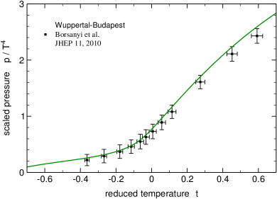
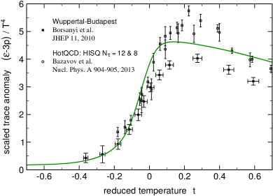
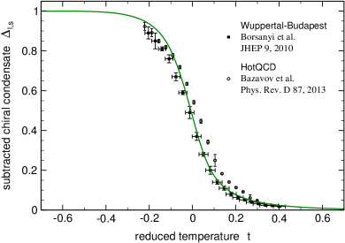
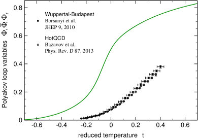
Figure 1: Pressure, trace anomaly, chiral condensate, and Polyakov loop as a function of $T$ in a PQM model Stiele (2014) (for this quantitative comparison, strange quarks have been taken into account) compared with the LQCD data of Refs. Borsanyi et al. (2010a, b); Bazavov (2013); Bazavov and Petreczky (2013).

In this figure, $t$ is the reduced temperature adjusted to the chiral crossover temperature $T_{c}$: $t=T/T_{c}-1$. The pressure plot, or the quark number density one, shows that at $T_{c}$ ($t=0$) quark degrees of freedom are liberated. But there are two mechanisms responsible for this liberation: the chiral restoration and the deconfinement transition. This can be easily studied in effective models since we have control on how these phenomena are coupled.

In Fig. 1, bottom left, it is possible to see that at $t=0$ chiral symmetry goes towards its restoration. There is a liberation of thermodynamical degrees of freedom simply because $m\rightarrow m_{0}$; hence, the quark Boltzmann factor has a bigger contribution to the pressure. This occurs at the chiral transition scale. On the bottom right panel, it is seen that the results for $\Phi$ from LQCD and PQM-model calculations do not agree. The same occurs in the PNJL model (see Ref. Torres-Rincon and Aichelin (2017)). The (statistical) deconfinement occurs at a higher temperature than in the PQM model (at $t=0$, the PQM model gives $\Phi\simeq 0.5$ whereas it is only $0.1$ for LQCD results). This means that the (statistical) deconfinement scales differ in LQCD data and in the PQM/PNJL model.

One subtlety concerning the Polyakov loop is that there are different order parameters. The standard order parameter is the expectation value $\langle\Phi\left[A_{0}\right]\rangle$. The functional dependence indicates that the Polyakov loop derives from the temporal component of the gauge field $A_{\mu}$. The expectation value of the latter $\langle A_{0}\rangle$ relates to another Polyakov-loop order parameter, $\Phi\left[\langle A_{0}\rangle\right]$.

LQCD results are for $\langle\Phi\rangle$ since this is the easily accessible quantity in these calculations. In Polyakov-loop extended effective models for QCD the Polyakov-loop potential is adjusted to LQCD results on $\langle\Phi\rangle$ in pure gauge theory while it is actually the gauge field that appears initially in the fermionic determinant (see Eq. (9)) which is then rewritten into a dependence on the Polyakov loop $\Phi$ in Eqs. (10) and (11). Both Polyakov-loop order parameters are related in general by $\langle\Phi\left[A_{0}\right]\rangle\leq\Phi\left[\langle A_{0}\rangle\right]$ Braun et al. (2010). This condition shows that the transition scales of both Polyakov-loop order parameters might differ with that of $\langle\Phi\rangle$ being larger than that of $\Phi\left[\langle A_{0}\rangle\right]$. The results shown in Fig. 1 are consistent considering this condition.

The origin of both these Polyakov-loop order parameters, their derivations, and their relation is discussed in detail in Ref. Herbst et al. (2015). The temperature dependence of $\Phi\left[\langle A_{0}\rangle\right]$ is calculated in continuum approaches such as the Functional Renormalization Group, with Dyson-Schwinger equations and the 2PI formalism as well as in the Hamiltonian approach and covariant variational approach, and in perturbative approaches. For pure gauge theory, available results on $\Phi\left[\langle A_{0}\rangle\right]$ in different continuum approaches are shown together with those for $\langle\Phi\left[A_{0}\right]\rangle$ of different LQCD calculations in Fig. 2.

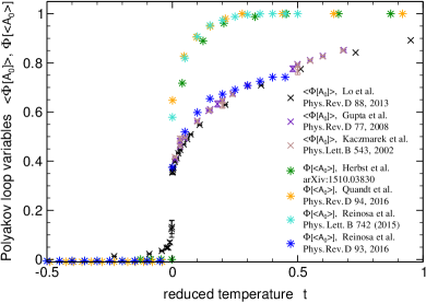
Figure 2: Comparison of the temperature dependence of the Polyakov-loop order parameter $\langle\Phi\left[A_{0}\right]\rangle$ on the lattice Kaczmarek et al. (2002); Gupta et al. (2008); Lo et al. (2013) and $\Phi\left[\langle A_{0}\rangle\right]$ in different continuum approaches Herbst et al. (2015); Quandt and Reinhardt (2016); Reinosa et al. (2015, 2016).

Interestingly enough, for the perturbation theory calculations, the leading-order result for $\Phi\left[\langle A_{0}\rangle\right]$ agrees with the results of the other continuum approaches while the evaluation of the next-to-leading-order result for $\langle A_{0}\rangle$ with the leading-order relation between the expectation value of the gauge field and the Polyakov loop $\Phi\left[\langle A_{0}\rangle\right]$ (see also Ref. Reinosa et al. (2016)) is very close to the LQCD results for $\langle\Phi\left[A_{0}\right]\rangle$.

The information given by LQCD calculations is that the scales of chiral-symmetry restoration and center-symmetry breaking do not match perfectly. In general, in the PNJL/PQM-model families, this scale separation is not achieved. Even worse, with common parametrizations as the one we use in the PNJL model ($T_{0}=190$ MeV), the scale hierarchy is inverted; see Fig. 7.

In effective models it is possible to have control over this hierarchy as we will show in the following. The shortcoming, however, is that the model output for the absolute temperature of the transitions will not be correct. This is a problem but not to the point of making the model meaningless. Indeed, in the spirit of Landau theory, two systems with the same universal behavior cannot be directly compared but they have to be compared relatively to a given scale. This is of course not a complete justification for what we will do in the following but it will illustrate which information can be obtained about some mechanism that is probably missing in the model. We recall that a scale adjustment was already done at the beginning of PNJL/PQM-model studies: for example, in Ref. Ratti et al. (2006) the scale $T_{0}$ was modified to get a complete agreement with the chiral transition temperature given by LQCD results.

So, the point is that we want to have in the model the correct scale hierarchy for the transitions. In both, PNJL and PQM models, we have two sectors to determine the respective scales, the NJL/QM one (fitted to chiral-symmetry breaking phenomenology in vacuum, a scale related to the strength of the condensate) and the gluonic one (fixed by pure gauge results at finite temperature with the scale $T_{0}$). The coupling is done via the covariant derivative but if we allow $T_{0}$ to vary then we can control the relative scales of the transitions. This is done in Fig. 3: we see that the correct hierarchy can indeed be achieved with $T_{0}\simeq 400$ MeV but the price to pay is that both, chiral and deconfinement transitions, occur at too high temperatures.

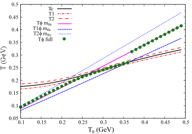
Figure 3: Chiral (black line) and deconfinement (magenta line and green dots) transition temperatures (together with the size of the transition regions $T_{1,2}$ and for deconfinement, the full (green) and fixed mass (magenta) calculations are presented) as functions of the pure gauge deconfinement scale $T_{0}$ for the PNJL model. We use the polynomial Polyakov-loop potential (Eq. (3)). We point out that we have the same feature with the $U_{Log}$ potential (Eq. (5)) but at a much higher scale.

The message is that some mechanism is missing to get the correct scale hierarchy and we should try to understand which mechanism would allow to have the same effect as our rather artificial increase of $T_{0}$. Since up to now no model can reproduce this fact, we probably need to look outside of the existing mechanisms of the PNJL/PQM models. Our guess is that introducing a minimal dynamics to the gauge sector Alba et al. (2014) may be the correct way.

We also notice that in PQM-model calculations, shown in Fig. 1, the pressure and quark density are probably a little bit overestimated for $t>0$ when compared to LQCD. If the correct scale hierarchy could be implemented, it is possible that the later liberation of quarks via statistical deconfinement could reduce this excess. This is a somewhat far fetched conclusion since the excess is low (statistically it seems to be a small but constant $\simeq$1 sigma deviation) and in the PQM model, mesonic degrees of freedom tend to survive in the QGP phase Herbst et al. (2014).

Finally, for what concerns this aspect of quark and Polyakov-loop correlations, we also notice in Fig. 3 that the transition for the full calculation for $\Phi$ from Eq. (15) and for the one keeping the mass $m$ at a fixed value $m_{\text{fix}}$ in Eq. (15) coincide, except when the difference between the chiral temperature and the fixed $m$ deconfinement temperature is smaller than about 25 MeV. This means that the order parameters $\Phi$ and the chiral condensate are weakly coupled by the mean-field equations because, except for a small 25 MeV $\ll\Lambda_{QCD}$ scale difference, the uncorrelated calculation (fixed $m$) gives the same result as the correlated one. We will discuss this kind of analysis in more detail in the next section.

At low $T_{0}$ the chiral transition is below its NJL/QM value (around 220 MeV) and it happens at a large (but below 1) value of the Polyakov loop while at high $T_{0}$ the chiral transition occurs for a small value (around zero) of the Polyakov loop. Thus, in the PNJL/PQM model the chiral transition always behaves differently from what happens in the NJL/QM model due to the back-reaction of the Polyakov loop, explaining the success of the model. The shortcoming of the model is essentially in the behavior of the Polyakov loop with respect to quarks but nevertheless, it seems that the action of the Polyakov loop on quarks, namely, the statistical confinement, captures most of the effect needed to correctly describe LQCD thermodynamics.

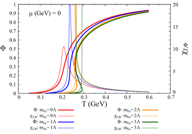
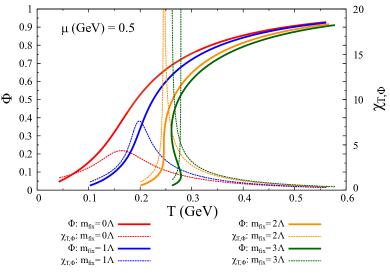
Figure 4: $\Phi$ and $\chi_{\Phi}=d\Phi/dT$ (Polyakov-loop susceptibility) as functions of $T$ for different values of the constituent quark mass $m$ in the PNJL model at zero density (left) and at finite density (right) where the Fermi momentum contributes to the kinetic energy. Varying the mass changes the strength of explicit breaking of the $\mathbb{Z}_{3}$ symmetry: when the mass is lower, the transition becomes a larger crossover. The higher the chemical potential, the higher the mass is needed to restore the symmetry and to have a first-order phase transition.

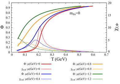
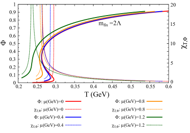
Figure 5: $\Phi$ and $\chi_{\Phi}=d\Phi/dT$ in the PNJL model as functions of $T$ for different values of the chemical potential at zero quark mass (left) and large quark mass $m=2\Lambda$ (right). A higher chemical potential implies a larger kinetic term and explicit $\mathbb{Z}_{3}$-symmetry breaking. A larger mass is required to get back a weak explicit breaking and a first-order phase transition.

The general conclusion is that quite certainly this class of models underestimates some effects for the lack of dynamical quark loop effect on the Polyakov loop. The only effect present is due to the presence of thermodynamical quarks (via the quark Boltzmann factor in the mean-field equation) that results from the minimal coupling $\bar{q}A_{\mu}q$. But, since $A_{\mu}$ is not dynamical this term will not generate quark loops in a diagrammatic approach ($A_{\mu}$ acts as an external constant gauge field only).

IV Dynamical thermal quarks effect

In this section we will consider the effect of the kinetic contribution of quarks in Eq. (15). At zero density ($\mu=0$) and with infinite quark mass, the second term disappears as it should. Indeed, quarks are then no more dynamical (they are quenched) and the system is in its pure gauge or Yang-Mills limit. The $\mathbb{Z}_{3}$ symmetry is then exact (for the grand potential) but spontaneously broken at $T>T_{0}$.

When quarks are considered dynamical again, by lowering their masses approaching the respective physical values, the $\mathbb{Z}_{3}$ symmetry gets also an explicit breaking term (see Secs. 2.2.2 and 2.3.2 in Ref. Stiele (2014)) due to the kinetic term in the Lagrangian. This mechanism can be understood in detail by solving the mean-field equations of the PNJL or PQM model, not self-consistently as usual, but simply by fixing $m$ to a given value $m_{\text{fix}}$ in Eq. (15), as already mentioned previously. In Figs. 4 and 5 we plot the behavior of the Polyakov loop for different masses, and hence changing the ratio between the mass energy $E_{m}$ and the kinetic energy $E_{k}$ of a quark: increasing the mass reduces the ratio $E_{k}/E_{m}$; when this ratio is zero (quenched quarks) the symmetry is restored. To better illustrate if there is a stronger or weaker explicit breaking of the $\mathbb{Z}_{3}$ symmetry, we use as Polyakov-loop potential a parametrization that has a strong first-order phase transition in the pure gauge sector (the $U_{Log}$ potential, Eq. (5)). If the transition becomes smoother (crossover like transition) it indicates that we have a stronger explicit breaking of the $\mathbb{Z}_{3}$ symmetry.

Figures 4 and 5 also show the impact of varying the chemical potential. Indeed, there is a contribution to the kinetic energy due to the Fermi momentum of quarks: increasing $\mu$ increases the ratio $E_{k}/E_{m}$ and the symmetry is more strongly broken. We will discuss further this effect in Sec. VI but for now, we focus on the zero density scenario where there is only one contribution to the kinetic energy.

We observe that a lowering of the mass term introduces a stronger explicit breaking of $\mathbb{Z}_{3}$ symmetry as seen by the large crossover obtained and the respective smooth Polyakov-loop susceptibility,

$$\left.\chi_{\Phi}=\frac{d\Phi}{dT}\right|_{\mu=0}.$$ (16)

On Fig. 6 we notice that, except when very close to the chiral transition (where $m$ changes quickly) the Polyakov-loop susceptibility is not much altered if the mass is kept constant. Thus, the transition properties are hardly affected by the exact value of the mass. Again, it is probable that this lack of sensitivity to the mass of the quark indicates a missing mechanism to account for the quark back-reaction on $\Phi$ because of the lack of dynamical quark loops in its calculation. For this reason, in the literature it is proposed that one adds phenomenologically more sources of back-reactions by using, for example in the entangled PNJL (EPNJL) model a scalar coupling $G_{S}$ that depends on $\Phi$ Sakai et al. (2010). Fitting this dependence is quite difficult (due to the lack of enough data) and some authors proposed to use the Roberge-Weiss transition at imaginary chemical potential Roberge and Weiss (1986) to fit this dependence. Other sources of back-reaction may be added by using a $\mu$-dependent gauge transition temperature $T_{0}(\mu)$ Schaefer et al. (2007) or even a $\mu$-dependent Polyakov-loop potential ${\cal U}(\Phi;T,\mu)$ Dexheimer and Schramm (2010).

We will not discuss further the EPNJL model but we would like to emphasize that it is interesting to understand the multiple aspects of back reaction already in the PNJL/PQM models before resorting to this type of model with reinforced back-reaction. Furthermore, models with many sources of back-reaction ($G(\Phi)$, $T_{0}(\mu)$) introduce many new parameters and it is not easy to parametrize them consistently without overestimating the back-reaction. In this regard, LQCD data at finite density would be very helpful or high density constraints (e.g., the measurement of the position of the CEP in heavy ion collision (HIC) experiments). It is interesting to note that LQCD data at finite imaginary chemical potential exists de Forcrand and Philipsen (2002); Wu et al. (2007); Nagata and Nakamura (2011); Cea et al. (2012); Bonati et al. (2019) and it is assumed that the continuation $i\mu\rightarrow\mu$ is analytic (this can be easily seen in the grand canonical potential of the PNJL/PQM model). Therefore, constraints at imaginary $\mu$ are relevant for models to be used at real $\mu$.

Let us mention a final comment on Fig. 6: as already discussed in Sec. II.3.3, the main effect of the Polyakov loop on the quark condensate is to obtain a steeper crossover transition and in the left panel of Fig. 6 we see that, indeed, when $\chi_{\Phi}$ (see Eq. (16)) is at its maximum it also introduces a dominant peak in $\chi_{\sigma}$.

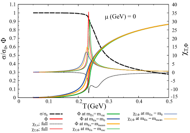
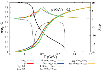
Figure 6: Quark condensate normalized to its vacuum value ($\sigma/\sigma_{0}$) and the Polyakov loop as a function of $T$ at zero and non-vanishing chemical potential (left and right). The Polyakov loop is computed either with a fixed mass ($m_{0}$, the mass in the vacuum $m_{vac}$ or $m_{mean}=\frac{m_{0}+m_{vac}}{2}$) or by fully solving the mean-field equations.

V Mean-field phase diagram

Using the techniques described in Costa et al. (2010b) we will now investigate the phase structure of a common two-flavor PNJL model, computed in this case with the logarithmic Polyakov-loop potential. To investigate the deconfinement transition we study the Polyakov-loop susceptibility at finite chemical potential,

$$\left.\chi_{\Phi}=\frac{d\Phi}{dT}\right|_{\mu},$$ (17)

and extract from it the characteristic pseudo-critical transition temperature associated to deconfinement, defined as the maximum of the susceptibility. In fact, we could also use $\chi_{\bar{\Phi}}=d\bar{\Phi}/dT$ to obtain the transition temperature being that $\chi_{\Phi}=\chi_{\bar{\Phi}}$ at $\mu=0$. At finite density $\Phi\neq\bar{\Phi}$ and the transitions temperatures obtained by the two susceptibilities are slightly different but very close to each other.

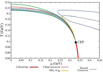
Figure 7: Phase diagram obtained in the ($T,\mu$) plane for the PNJL model. The red dashed and solid lines represent the chiral crossover and critical line. The blue dashed line marks the deconfinement crossover and is within the transition region which is outlined by the blue solid lines (and defined within the main text). The yellow line represents the minimum of the Polyakov-loop susceptibility, $\chi_{\Phi}$. The transition region of the chiral crossover is within the green solid lines.

Some details of the numerical calculations for a similar model, which are not of importance for our quantitative discussions, can be found in Biguet et al. (2015). To obtain the susceptibilities the “easy way” is to compute them as numerical derivatives. This is both inefficient (it is quite long since for each step in temperature the mean-field equations have to be solved several times) and inaccurate. The inaccuracy will show up as a numerical fluctuation in the transition line plot which shows the maxima of the susceptibilities. A more accurate and faster way is to compute analytically (or at least semi-analytically in the sense that the non analytic thermal integrals are kept as numerical integrals) all first- and second-order partial derivatives of the grand potential with respect to the order parameters and the thermodynamic parameters $T$ and $\mu$ and then combine them to get the desired susceptibilities (see Wagner et al. (2010); Biguet et al. (2015)).

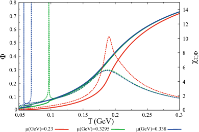
Figure 8: Polyakov loop, $\Phi$, and its susceptibility for chemical potentials below the one of the chiral CEP in the PNJL model (red), at the CEP chemical potential (green) and above the CEP chemical potential (blue).

Results for the order parameters $m$ and $\Phi$ are presented in Fig. 7. Concerning the chiral properties, they behave as discussed in the introduction and we observe a first-order phase transition line that starts at zero temperature and ends with increasing temperature at the CEP, where a second-order phase transition occurs at ($T^{\mathrm{CEP}},\mu^{\mathrm{CEP}}$), continued by a crossover for further increasing temperatures and decreasing chemical potentials.

For what concerns the deconfinement transition we see that for chemical potentials $\gtrsim 250\,\mathrm{MeV}$ $\chi_{\Phi}$ has several maxima or divergent peaks (Fig. 8) but the order parameter always shows a crossover transition. Indeed if we look at the Polyakov-loop susceptibility in Fig. 8, we see that there is a divergence at the chiral transition temperature but physically this is not the signal of the deconfinement transition. We see that at this chiral first-order transition, $\Phi$ increases only about 5% and stays below 0.2: this is not a (first-order) deconfinement transition because quarks are still statistically confined when $\Phi=0.2$. There is also a bump in $\chi_{\Phi}$, and there $\Phi$ changes between 0.4 and 0.7 and the system reaches the statistically deconfined phase. Hence, we will consider the temperature at the maximum as the one of the deconfinement crossover.

For the sake of completeness, we also have plotted in the phase diagram of Fig. 7, besides the maximum of $\chi_{\Phi}$, its inflection points (which estimate the “extent” of the crossover region) and also the minimum of $\chi_{\Phi}$, when it exists, between the bump of the deconfinement crossover and the peak of the first-order phase transition of chiral symmetry.

It should be noted that both transitions appear to be strongly correlated below $\mu\lesssim 250\,\mathrm{MeV}$ and then become uncorrelated at higher chemical potentials, indicating the mutual influence between chiral and deconfinement sectors. The topic of the quark - Polyakov-loop correlation deserves therefore special attention as discussed in Sec. II.3.2.

VI Quark condensate and Polyakov-loop correlation

Here we continue our study of the finite density (finite chemical potential) region using the PNJL model and we compare results obtained with and without fixing the mass. At zero density, the pseudo-critical transition temperatures for the partial chiral-symmetry restoration and deconfinement coming from LQCD results are very close, differing by approximately 20 MeV Borsanyi et al. (2010a). At finite density the status is not clear (different model parametrizations give very different results). Experimentally, there is a lack of high temperature and density experiments. Furthermore, it is also difficult to extract information about the chiral sector only or the deconfinement sector only.

We will study the high density regions and the possible opening of a new phase near the CEP (this feature is model dependent and will eventually disappear by considering a $T_{0}(\mu)$ parametrization, see Ref. Kahara and Tuominen (2010)). From Fig. 7 and starting at $\mu=0$, it is seen that as the chemical potential increases the chiral and the deconfinement crossover lines approach each other as one approaches the CEP. Then they merge for $\mu<\mu^{CEP}$. This property of the QCD phase diagram has been used to estimate a lower bound for the chemical potential at the CEP (see for example Fig. 1 of Ref. Endrodi et al. (2011)). Still, near the CEP, chiral and deconfinement transitions decouple.

In Fig. 9 the Polyakov-loop susceptibility is computed (using the polynomial Polyakov-loop potential) with the full mean-field equations, and with a mass fixed to the mean value of its value in the vacuum and the current quark mass $m_{0}$, $m_{mean}=\frac{m_{0}+m_{vac}}{2}$ (dashed lines). We can see that for a chemical potential that gives a first-order phase transition for the chiral transition (red full line), there is a peak in the Polyakov-loop susceptibility at the chiral transition. Having in mind the discussion of the previous section, at this peak, the Polyakov-loop only varies from 0.2 to 0.3. There is also a bump in $d\Phi/dT$ at higher temperatures and around this bump, $\Phi$ goes from 0.4 (essentially confined phase) to 0.7 (essentially deconfined). Our interpretation is the following: the peak in $\chi_{\Phi}$ is not a sign of a first-order deconfinement transition because the value of the Polyakov-loop remains small. But there is a smooth crossover towards the deconfined phase at higher temperatures (at the bump). These two transitions are relevant because they are related to physical effects of the thermodynamic potential we are using, the grand canonical potential: the peak (the chiral first-order transition) manifests itself as a singularity of the derivative of the grand potential; the bump gives a small region where there is a sharp increase then decrease (but continuous) of the derivative of the grand potential with respect to the order parameters. It is a manifestation of the deconfinement crossover. These two transitions show their imprint on the pressure as we will discuss in Sec. IX where a plot of the relative pressure difference (compared to the Stefan-Boltzmann one, Fig. 12) clearly shows that both transitions delimit three distinct regions in the phase diagram. This interpretation opens the possibility to describe an intermediate phase, that we call confined chirally restored phase (CCS). Indeed, it can be explicitly shown that in this phase, quark matter is still (statistically) confined. However, we postpone the detailed discussion to Sec. IX.

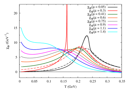
Figure 9: Polyakov-loop susceptibility as a function of $T$ for different chemical potentials (given in GeV). The dashed lines are the calculation with fixed $m=m_{mean}$ (see definition in the main text); the full line is the fully consistent calculation. Notice in the region of low temperature that for high chemical potentials, $\chi_{\Phi}$ has no more maximum.

In Fig. 9 it can also be seen that when using a constant mass, the chiral peak in the Polyakov-loop susceptibility disappears (dashed lines). This is understandable since we argued that there is not a significant variation in $\Phi$ at these temperatures but only a very strong mass change that creates the large derivative. $\Phi$ itself does not vary much since we saw that it is not very sensitive to mass variations below $\Lambda_{QCD}$.

When the mass is fixed the maximum is approximately the same as in the full calculation, not taking into account the possible divergent peak. This shows that taking $m$ fixed really allows to decorrelate the chiral condensate effects because the shape of the Polyakov-loop susceptibility does not change significantly when the mass varies strongly (in the interval $T\in[100\text{MeV},250\text{MeV}]$ the mass goes approximately from 320 MeV to 150 MeV). All the remaining effects are only due to the chemical potential, an aspect that we will discuss in the next section about the Fermi momentum effect.

Another important aspect is that the use of a fixed mass, $m_{\text{fix}}$, is also very useful numerically. If we want to draw a phase diagram, but the exact behavior of the Polyakov loop near the CEP is not so relevant, we can use this trick and get a faster algorithm since only two mean-field equations have to be solved. This method can be helpful even to compute the full solution: it can greatly increase the calculation speed if we start to compute the approximated $m_{\text{fix}}$ value and then incorporate it in the solving algorithm for the full equations. This kind of algorithm (root polishing when the approximate solution is known) is particularly helpful when the dimension of the problem increases (here three dimensions since there are three mean-field equation equations; including the strange sector and without isospin symmetry it would be five dimensions).

It is possible to qualitatively compare both methods, fixed mass and full calculation, by looking to the phase diagram in Fig. 10 (here the Polyakov-loop potential is the polynomial one but qualitatively our results are independent of the choice of this potential). The conclusion is that except in the region of the CEP it does not differ from the previous one found in Fig. 7, Sec. V. The extra features will be discussed in the next section since they concern large density effects.

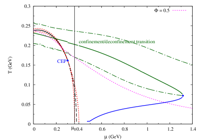
Figure 10: The PNJL-model phase diagram using a constant mass to compute $\Phi$. Other features are added: the magenta dashed line represents $\Phi=0.5$; the blue line is given by the minimum of the Polyakov-loop susceptibility. When this minimum and the maximum (the crossover curve, represented by the green line) meet, it is no more possible to strictly define even a crossover transition at higher chemical potentials. $\mu_{0}$ is the chemical potential where $\chi_{\Phi}(T=0)$ starts to be non zero, see Fig. 9. The red dashed lines represent the transition region and metastable region of the chiral transition and the dash-dotted green lines the transition region of the deconfinement crossover.

VII Fermi momentum effect

In the previous section, we have seen in detail one important aspect of the chiral transition/deconfinement transition correlation by carefully considering the effect of the quark masses on the field equations. As mentioned, there is another quark effect in the mean-field equations via the quark chemical potential, which originates from a non zero Fermi momentum of the quarks.

Because of the covariant derivative and the inclusion of $\mu$ in the Lagrangian, there is a dependence on $\mu$ in Eq. (15) that can have a strong effect on the system. In fact, the Fermi energy will act exactly as any kinetic energy (in the Lagrangian $\mu\gamma^{0}$ acts as $\partial_{0}\gamma^{0}$) and increases the explicit breaking of $\mathbb{Z}_{3}$ symmetry. As seen in Fig. 9, where we computed $\chi_{\Phi}$ for several chemical potentials, at some point, the breaking of the symmetry is so strong that the transition cannot be defined even as a crossover anymore (at least according to our definition). From the moment that the Polyakov-loop susceptibility does not have a maximum anymore, our interpretation is that the transition goes so fast from $\Phi=0$ to $1$ (and without the characteristic of a crossover transition where correlation lengths quickly increase then decrease) that we can almost say that the system is deconfined even at zero temperature (in Fig. 10, $\Phi$ is already 0.5 at $T=50$ MeV for large values of $\mu$). $\Phi$ is forced to be zero at zero temperature but in the large $\mu$ limit, $\Phi=1$ at any non-vanishing temperature. Hence, the model basically tells us that, apart from a small missing ingredient, a form of effective deconfinement only induced by the density is possible. This missing ingredient is again probably related to quark back-reaction on the gauge fields.

Here, we want to point out that it is quite remarkable that, in their simple versions, the PNJL and PQM models already allow a deconfinement transition caused only by the density (with a small temperature), without any sort of ad hoc back-reaction added.

In the phase diagram presented in Fig. 10, more relevant features can be found. It is interesting to have an idea of the value of the order parameter, $\Phi$, with respect to the transition lines, so we add the $\Phi=0.5$ characteristic line (magenta dashed curve). More importantly, we show in this diagram that there is a kind of “crossover end point” in this model calculation. At very high $\mu$ the explicit breaking of $\mathbb{Z}_{3}$ symmetry is so strong that $\chi_{\Phi}$ has no longer a maximum (except at $T=0$, see also Fig. 9). Somehow, this explicit symmetry breaking is dominant in the Lagrangian and after this point it is no longer possible to talk about a transition, even a crossover one. The symmetry is completely destroyed by this breaking term.

As a conclusion, we emphasize that only the careful assessment of the sources of correlations in the mean-field equations allowed us to see those effects. We advocate that even in this simple model some mechanisms, such as the Fermi momentum action, can be seen. The use of more realistic models (e.g., SU(3) PNJL/PQM models) would also be interesting to get more faithful results. However, we think that those models, with many interplays between physical sectors whose contributions are controlled by parameters adjusted to phenomenology, are complementary to the simpler models and both have their merit.

VIII Combined effects of chiral condensate and Fermi momentum

To complement our discussion on the influence of changing the chiral condensate (by varying $m$) and the Fermi momentum (by varying $\mu$) on $\Phi$, Fig. 11 presents the results for the deconfinement temperature obtained when varying both $\mu$ and the fixed mass $m_{\text{fix}}$.

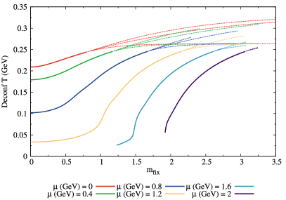
Figure 11: Deconfinement characteristic temperature as a function of the fixed mass and for different chemical potentials. The full line is the crossover temperature and the dotted lines are the metastable limit of a first-order phase transition.

Taking $\mu=0$, the deconfinement transition for $m_{\text{fix}}=0$ is a crossover with a transition temperature that is about the same as the chiral one (for this model parametrization it is about 220 MeV). This corresponds to the usual situation of the PNJL/PQM model when both transitions almost coincide at zero density. As already explained when discussing Fig. 4, by increasing the mass (thus decreasing the explicit $\mathbb{Z}_{3}$-symmetry breaking) the temperature increases until it reaches a value where the crossover becomes a first-order phase transition, at a temperature of about 270 MeV (which is the value of $T_{0}$ in this parametrization).

Now, looking at $m_{\text{fix}}=0$ and increasing $\mu$, we see a lowering of the deconfinement crossover temperature until a value where the crossover cannot be defined anymore. The symmetry breaking induced by the Fermi momentum is so strong that after this point, $\mathbb{Z}_{3}$ is no more a valid symmetry of the model.

Finally, by varying both $\mu$ and $m_{\text{fix}}$ it is always possible to go to a first-order phase transition if the mass is sufficiently high compared to $\mu$ in order to counteract the explicit breaking of $\mathbb{Z}_{3}$ symmetry.

IX Confined chirally restored (CCS) phase

In this section we will take a closer look to the CCS phase, a phase where chiral symmetry and deconfinement are decorrelated.

In PNJL/PQM models it is always necessary to remember that quarks are not confined in the strict sense and when we talk about confinement we mean statistical confinement as given by the definition in Sec. II.3.3. These types of models cannot tell us the true nature of quark confinement.

To explore the CCS phase, we want to count the number of thermal quark degrees of freedom (the only one affected by statistical confinement). For this reason we need to subtract the quarks in the vacuum, present due to the lack of confinement (we have seen that their contribution is quite reasonable by looking to the quark number density in Sec. II.3.3). Hence, we calculate a relative pressure difference by subtracting the pressure at zero temperature and normalizing it to the Stefan-Boltzmann pressure:

$$\Delta P\equiv\frac{P(T,\mu)-P(T=0,\mu)}{P_{SB}(T,\mu)-P_{SB}(T=0,\mu)}.$$ (18)

This quantity is adequately related to the thermal quark degrees of freedom and indeed it shows signs of statistical confinement in the CCS phase (see Fig. 12).

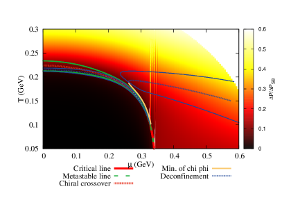
Figure 12: Relative pressure difference as defined in Eq. (18) (color map), in the ($T,\mu$) plane, superimposed on the PNJL-model phase diagram of Fig. 7.

In the hadronic phase, $\Delta P$ is zero (the black region), meaning that the PNJL/PQM model will not thermodynamically create any quarks in the hadronic phase (besides those already present in vacuum). In the QGP phase (the yellow region), thermal quarks are very active thermodynamically. Finally, in the CCS phase a quite stable “plateau” (the red/orange region at large chemical potential and small temperature) at around 0.2 is found. At a given (small) temperature, there is a discontinuous jump from 0 to 0.2 when increasing $\mu$ across the first-order phase transition. So, in the CCS phase some quarks have been liberated by the system due to the chiral transition but their contribution to thermodynamics remains low. It seems that in this phase, where the chiral symmetry is restored, the model tells us that quarks still are far from being asymptotically free. Phenomenologically, this could have rather important effects on experimental observables in HICs (viscosity, hadronic abundances, etc). If this hypothetical phase exists in QCD, the PNJL/PQM model cannot say if quarks are really confined (no asymptotic states) or if they are deconfined but the model predicts that the interaction is still strong allowing the existence of mesonic resonance as we will show. Performing the same calculation in the pure NJL/QM model, i.e. without statistical confinement, one observes at small temperature that $\Delta P$ has the same jump at the chiral transition and then increases slowly without a “plateau” behavior.

It is also relevant to notice that, at those densities, an important missing effect is the presence of diquark condensates. The strange sector is also important and it deserves further investigation.

To confirm this finding and that it may lead to significant differences in HICs, we study a more direct observable, namely, we check if mesonic probes act as it is expected in a confined but chirally symmetric phase.

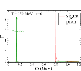
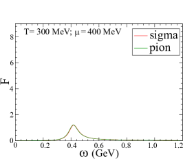
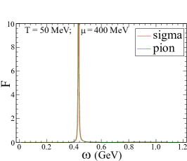
Figure 13: Pion and sigma spectral function in the PNJL model for the hadronic phase (left) and the QGP phase (middle). Confining regime: $\sigma$ is a narrow resonance; the chiral symmetry is broken and $\langle\bar{q}q\rangle\neq 0$; $\Phi\simeq 0$. Deconfinement: $\sigma$ and $\pi$ spectral functions are almost the same as an uncorrelated $\bar{q}q$ pair; the chiral symmetry is restored and $\langle\bar{q}q\rangle\simeq 0$; $\Phi\neq 0$.
Right panel: Pion and sigma spectral function in the CCS phase. The system is in the statistically confined phase since $\sigma$ and $\pi$ are still narrow resonances. But chiral symmetry is restored: $\langle\bar{q}q\rangle\simeq 0$; $\Phi\simeq 0$.

We compute in the PNJL model the spectral functions (see Ref. Hansen et al. (2007)) in the meson to quarks channel at zero momentum and show them in Fig. 13. The finite width of the sigma in vacuum indicates that quarks are not confined (this channel is open) but there is a strong interaction and thus it is a sharp resonance.

The expected behavior for mesons in a CCS is observed in the same Fig. 13: chiral symmetry is effectively restored when the sigma and pion spectral functions essentially coincide Hansen et al. (2007) but the statistical confinement is still strong as can be seen by the fact that their width is small (right panel) when compared to the fully deconfined phase (central panel).

Finally, as already mentioned, other parametrizations, for example a $T_{0}(\mu)$, will essentially close this CCS phase Kahara and Tuominen (2010). Yet, we think it is still interesting to try to understand better the CCS phase. We also think that $T_{0}(\mu$) is a too strong a priori generalization to introduce in the model. This dependence is justified theoretically in Ref. Schaefer et al. (2007), where it is argued that this generalization is needed, because otherwise the confinement-deconfinement transition has a higher pseudo-critical temperature than the chiral transition, which is an unphysical scenario since QCD with dynamic massless quarks in the chirally restored phase cannot be confining because the string breaking scale would be zero. However, the problem is that it is poorly constrained. Using this parametrization, the hypothesis is basically that deconfinement and chiral restoration coincide. Of course, the CCS phase will then not exist anymore but in our opinion this is not a sufficient argument against the existence of a CCS phase in general. It can eventfully be an argument against the CCS phase only if this a priori generalization is correct but this has to be put on a firmer basis and, in particular, be better constrained.

In the meantime, we think that it is still interesting to consider models with a CCS phase even if in the future it will be contradicted by experimental data, which will be the ultimate judge. Anyway, it is still a nice exercise to see what physical information can be gathered by using effective models.

X Conclusions and outlook

At the beginning of this work we present the current status on how accurately effective models based on the restoration of chiral symmetry and on the breaking of center symmetry (to describe the deconfinement transition of QCD) can reproduce the results coming from LQCD calculations. Based on the observation that there is a substantial quantitative difference in the temperature dependence of the Polyakov loop relative to that of the chiral condensate, we have analyzed several aspects of the correlation between the chiral sector and the Polyakov loop.
By examining how the pseudo-critical temperatures for chiral and the Polyakov-loop transitions depend on the critical scale of the Polyakov-loop potential, $T_{0}$, we see that the correct ordering of chiral and Polyakov-loop transitions (and their difference in temperature), as given by LQCD calculations, can be achieved with a $T_{0}$ larger than the one given by pure gauge theory (270 MeV). The absolute temperature scale of the QCD transition would then be larger than the one in LQCD. In the spirit of Landau theory, however, effective models should be considered on relative scales.

For studying the effect of the kinetic contribution of quarks to the correlation between quarks and the Polyakov loop, we compared the behavior of the latter between calculations using a self-consistent medium-dependent quark mass and for several values of constant quark masses, $m_{\text{fix}}$. Except very close to the chiral transition (where $m$ changes quickly), the Polyakov-loop susceptibility is not much altered by keeping the mass constant at the value $m_{mean}$ so that even the transition properties are almost not affected by the precise value of the mass. We interpret this lack of sensitivity to the mass of the quark as a sign of a missing mechanism to take into account the quark back-reaction on the Polyakov loop due to the lack of dynamical quark loops in its calculation. Comparing the Polyakov-loop susceptibility for a medium-dependent and a constant mass at finite density allows to disentangle a smooth crossover proper to the breaking of center symmetry from a peak in the susceptibility introduced purely by a chiral first-order phase transition but at which the value of the Polyakov loop remains small, so in the confined regime. This picture opens the possibility to discuss an intermediate phase, which, in our model, is a confined chirally restored phase. Probing the number of thermal quark degrees of freedom within this phase, indeed, one sees signs of statistical confinement with a quite stable “plateau” where some quarks have been liberated due to the chiral transition but where their contribution to thermodynamics remains low. Furthermore, meson spectral functions behave as they are expected in a confined but chirally symmetric phase: the sigma and pion spectral functions essentially coincide but their width is small.
Another contribution to the correlation between quarks and the Polyakov loop at non-vanishing density comes from the fact that the Fermi energy acts exactly as any kinetic energy and increases the explicit breaking of center symmetry. From some large chemical potential on this explicit breaking of the symmetry is so strong that the Polyakov-loop susceptibility does not have a maximum anymore except at $T=0$. Hence, apart from a missing ingredient, deconfinement induced only by the density seems to be realizable within the model. This missing ingredient is again probably related to quark back-reaction on the gauge fields.

Overall, the goal of this work is to shed light on some lesser known aspects of Polyakov-loop–extended chiral models to motivate certain paths for future improvements and detailed quantitative analysis.