University at Buffalo, The State University of New York, Buffalo 14260, USA
at Next-to-Next-to-Leading Order Accuracy
Abstract
We present the calculation of the decay at next-to-next-to-leading order (NNLO) accuracy in QCD. We treat the bottom quarks as massless with a non-zero Higgs Yukawa coupling . We consider contributions in which the Higgs boson couples directly to bottom quarks, i.e. our predictions are accurate to order . We calculate the various components needed to construct the NNLO contribution, including an independent calculation of the two-loop amplitudes. We compare our results for the two-loop amplitudes to an existing calculation finding agreement. We present additional checks on our two-loop expression using the known infrared factorization properties as the emitted gluon becomes soft or collinear. We use our results to construct a Monte Carlo implementation of and present jet rates and differential distributions in the Higgs rest frame using the Durham jet algorithm.
1 Introduction
The discovery of the Higgs boson Aad:2012tfa ; Chatrchyan:2012xdj has set a large part of the agenda in high energy physics for the foreseeable future. Of primary concern is the need to determine the properties of the Higgs boson in relation to the predictions of the Standard Model (SM). This is mainly achieved through measurements of the couplings of the Higgs boson to the other SM particles and the Higgs coupling to itself. The Higgs self-coupling is of particular interest, since it is intimately linked to the electroweak symmetry breaking potential, the form of which is still unconstrained through measurements of the Higgs mass alone (although its remaining properties are predicted in the SM). Any additional physics beyond the Standard Model (BSM) could lead to significant changes in the shape of the electroweak symmetry breaking potential, and thus lead to deviations from the SM predictions.
Measuring the properties of the Higgs boson is an ongoing task. In regards to that, the LHC has already achieved a remarkable precision with existing Run II measurements and will significantly improve upon these results over the course of the next decade. Plans are afoot for future colliders beyond the LHC (FCs) and a particularly appealing prospect regarding Higgs precision physics is the construction of a lepton collider. Due to the clean experimental conditions, future lepton colliders should be able to probe the properties of the Higgs boson down to per-mille level accuracy Baer:2013cma ; Gomez-Ceballos:2013zzn ; Abada:2019zxq .
The Higgs boson decays predominately to bottom quark pairs ), and therefore a large part of the experimental program at the LHC and putative FCs consists in measuring the properties of this decay. At the LHC the process can be accessed through associated production channels followed by a subsequent decay Aaboud:2018zhk ; Sirunyan:2018kst or directly, by using jet substructure techniques and by looking in the high- channel Sirunyan:2017dgcx , where the backgrounds can be controlled to such a level as to make this measurement a possibility. In both situations precise predictions are mandatory to ensure that theoretical calculations have a similar or smaller uncertainty than the experimental counterparts. This will become even more pressing at an FC, for which historical measurements from LEP for jets already show that the level of experimental uncertainty will be very small indeed.
Given its importance for LHC physics, the study of Higgs plus multi-parton production has received significant theoretical attention over the last couple of decades. Working within the effective field theory, in which the top quark is treated as infinitely heavy, the production of a Higgs through gluon fusion is known to N3LO in QCD Anastasiou:2015ema ; Anastasiou:2016cez . Recently, differential predictions at this order have been computed using the method of subtraction Catani:2007vq ; Cieri:2018oms and analytically for the rapidity distribution Dulat:2017prg ; Dulat:2018bfe . In order to compute differentially at N3LO, must be available at NNLO, at NLO, and at LO. These computations have all been performed Boughezal:2013uia ; Chen:2014gva ; Campbell:2006xx 111Indeed, is also available at NLO in QCD Cullen:2013saa .. Of particular note for this work is the calculation of at NNLO, which requires the analytic computation of partons in the EFT Gehrmann:2011aa . The related process in which the Higgs boson decays to three partons via a tree-level coupling to -quarks has been less well-studied in the literature. Attention has naturally been focused on the process which has been studied at NLO Braaten:1980yq and NNLO Anastasiou:2011qx ; DelDuca:2015zqa ; Bernreuther:2018ynm , and inclusively is known to Baikov:2005rw . No complete NNLO prediction for is available, although a calculation of the two-loop amplitudes has been presented Ahmed:2014pka .
The aim of this paper is twofold. Firstly, we perform an independent computation of the two-loop amplitudes for which have been presented in the literature in Ref. Ahmed:2014pka . Secondly, we use these results to produce a NNLO Monte Carlo code for the process. The primary goal is to establish whether we can effectively integrate out the additional jet at NNLO. By successfully doing so, we open up the possibility of studying decay at N3LO. We perform this calculation in a companion paper Mondini:2019gid .
Our paper proceeds as follows. In Section 2 we give a general overview of the calculation, while a detailed discussion of our two-loop computation is presented in Section 3. We discuss the results of our Monte Carlo implementation of in Section 4. After drawing our conclusions, we present the full analytic results of our two-loop amplitudes in the appendix.
2 Overview of the calculation
2.1 General overview
In this paper we consider the decay of a Higgs boson to a bottom quark pair and an additional jet at NNLO in QCD. In perturbation theory up to NNLO the partial decay width is expanded as follows:
| (1) |
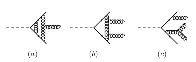
The above formula introduces the notation we will use in this paper: defines the partial width at order in perturbation theory, while defines the coefficient which enters the expansion for the first time at this order. Representative Feynman diagrams for our NNLO calculation are shown in Fig. 1. Specifically, at NNLO we need to compute two-loop amplitudes for , one-loop amplitudes for and (including identical-quark terms ), and tree-level amplitudes for , , and .
Radiative corrections to the decay were first studied nearly forty years ago Braaten:1980yq , when it was shown that there are sizable differences between calculations in the “massless theory”, in which the -quark mass is dropped in the phase space and kinematics but kept in the -quark Yukawa coupling, and in the full theory, in which the -quark mass is retained throughout. These differences were shown to be primarily due to logarithms of the form . It was also discussed how these effects can be reinstated in the massless theory by running the -quark mass in the Yukawa coupling. Using the -quark mass evolved to the Higgs scale in the massless theory results in much smaller differences between the two theories. This was shown explicitly in Ref. Chetyrkin:1996sr , where the inclusive decay rate was computed up to order including power-suppressed corrections of the form up to order . The numerical evaluation of the decay rate shows that at each order in the mass corrections are at the per-mille level relative to the massless contribution at the same order and that they are also smaller than the massless corrections at the next order in perturbation theory. It is therefore advantageous and theoretically convenient to work in the massless limit, due to the reduced complexity of higher-order Feynman diagrams. In the massless theory the inclusive partial width for the decay channel is currently known to an impressive accuracy Baikov:2005rw . The form factor for at three loops is also known Gehrmann:2014vha , so that, once a NNLO calculation of is complete, all of the component pieces for at N3LO are available.
In this paper we will therefore work in the massless theory in which the -quark mass is dropped from the phase space and kinematics, but kept in the Yukawa coupling with the -quark mass run to the Higgs scale. As mentioned above, a result of the massless theory assumption is that it simplifies the calculation by reducing the number of Feynman diagrams which must be included at one and two loops. We refer in particular to diagrams in which the Higgs boson couples indirectly to the -quarks, for which example topologies are shown in Fig. 2. At these diagrams interfere with the respective tree-level amplitudes for and for the two-loop and one-loop calculations respectively. A simple helicity argument indicates that these interference terms are zero. In the and tree-level amplitudes the scalar Higgs boson couples directly to the two (massless) quarks, which therefore must have identical helicity assignments (both positive or negative). On the other hand, the diagrams in which the Higgs couples implicitly to the quarks as shown in Fig. 2 always result in the final-state pair coupling directly to a gluon. This vertex requires that the fermions have opposite helicities, and therefore there is no combination that allows non-zero interference terms to exist, resulting in no net contribution from these diagrams at NNLO (the box squared would first enter at ).

A slight subtlety arises when we consider the one-loop triangle diagram in which the Higgs boson couples indirectly to the bottom quarks (i.e the left diagram in Fig. 2 with no additional gluon exchanged in the loop). This diagram would self-interfere at and is therefore not excluded from our NNLO calculation by the argument presented above. However, the trace over the fermion loop for this diagram contains five matrices and hence this term vanishes in the massless theory. In order for this diagram to give a non-zero contribution, the quark mass must be retained in the loop. This is the case when the loop particle is a top quark, and hence there exists a top Yukawa contribution which first enters at in our calculation. Schematically, the perturbative expansion of the decay width in the full theory is of the form:
| (2) |
where and are the bottom and top Yukawa couplings respectively. From the arguments given above it is clear that in the full theory the interference terms and are suppressed by the bottom-quark mass (since a helicity flip is needed to make a non-zero interference term). However, since the top Yukawa coupling is large, these mixed terms are of phenomenological relevance. Specifically, in an effective theory in which the top-quark loop is integrated out, the term contributes to around 30% of the coefficient Primo:2018zby . For our theoretical setup, the mixed term and are exactly zero. In addition, at the pure top contribution mentioned above needs to be included. Indeed, while formally this term enters the perturbative expansion as a one-loop squared contribution, the higher-order corrections are known to be large (and well-studied in the EFT approach). This means that for a good phenomenological description higher-order terms proportional to should be included as well. The IR properties of this piece are further complicated by the presence of collinear singularities as the pair becomes unresolved (in the massless theory) since this piece factors onto a different LO term (). In this paper we drop the term for two reasons. Firstly, we are interested in the theoretical computation of the terms (which is new), while the study of the contribution has received significant attention in the literature through the various studies of at the LHC. Secondly, we wish to use this computation to perform the N3LO calculation of the terms for . We leave the inclusion of the top Yukawa contributions to a future study, while we remind the reader that these contributions should be included before a complete phenomenological study is performed.
2.2 -jettiness slicing
In order to regulate the IR divergences present in our NNLO calculation we employ the -jettiness slicing method Gaunt:2015pea ; Boughezal:2015dva . Since there are three partons in the final state at LO we use the 3-jettiness variable to separate our calculation into two pieces. For a parton-level event the 3-jettiness variable Stewart:2010tn is defined as follows:
| (3) |
where the index runs over the partons in the phase space (with momenta ), while represent the momenta of the three most energetic jets, clustered in our case with the Durham jet algorithm Brown:1990nm ; Catani:1991hj . are the hard scales in the process, which are typically taken to be with the energy of the -th jet. We then introduce a variable that separates the phase space into two regions. The region contains all of the doubly-unresolved regions of phase space and here the partial width can be approximated with the following convolution, derived from SCET Stewart:2010tn ; Stewart:2009yx :
| (4) |
In the above equation the terms correspond to the jet functions which describe collinear emissions, denotes the soft function for three colored partons, and is the process-specific hard function. The explicit expressions for the jet functions needed for our NNLO computation can be found in Ref. Becher:2006qw . For the soft function, we use the results for the 1-jettiness soft function with arbitrary kinematics computed in Ref. Campbell:2017hsw (see also Ref. Boughezal:2015eha ). The calculation of the hard function for this process is one of the primary aims of this paper and is discussed in Section 3. In order for the approximate form of the partial width in Eq. (4) to be accurate, should be taken as small as possible to minimize the power corrections which vanish in the limit .
2.3 The contribution
Since any doubly-unresolved contribution resides in the region , the region corresponds to the NLO calculation of . The methods to compute one-loop expressions are by now well-established so we do not spend significant time on them here. In this section we limit ourselves to a brief description of the computation. One-loop amplitudes are computed analytically using the generalized unitarity approach Bern:1994zx . Specifically, quadruple cuts are used to compute box coefficients Britto:2004nc , triple cuts are used to compute the triangle coefficients Forde:2007mi , double cuts are used to compute bubble coefficients Mastrolia:2009dr , and the rational pieces are computed using -dimensional unitarity techniques as outlined in Ref. Badger:2008cm . Our calculation is checked numerically using the -dimensional unitarity algorithm presented in Ref. Ellis:2008ir . The resulting expressions are rather compact, with a similar level of complexity to the amplitudes presented in Ref. Badger:2009hw . Tree-level amplitudes are computed using the BCFW recursion relations Britto:2005fq and all tree-level amplitudes present in the calculation have been checked against Madgraph Alwall:2011uj . Finally, IR divergences in the NLO calculation are regulated using Catani-Seymour dipole subtraction Catani:1996vz .
3 Hard function for at NNLO
In this section we describe the calculation of the hard function of Eq. (4) for the process at NNLO accuracy. We define the hard function as a perturbative series in powers of the renormalized strong coupling at the renormalization scale :
| (5) |
The LO, NLO, and NNLO coefficients of the hard function are
| (6) | ||||
| (7) | ||||
| (8) |
where is the -renormalized -loop amplitude in the notation of Ref. Becher:2013vva . The calculation of with is described in the following sections.
3.1 Notation and kinematics
We consider the decay
The Mandelstam invariants for this process are defined as
and satisfy with the mass of the Higgs boson. We also introduce the dimensionless quantities
| (9) |
which satisfy , , , and .
We follow the notation introduced in Ref. Ahmed:2014pka , in which the unrenormalized amplitude for is written in terms of two tensor structures:
| (10) |
where is the bare strong coupling constant, is the bare bottom Yukawa coupling, is the color matrix with gluon color index and quark indices and , and is the gluon polarization vector. Finally, the tensors and are defined as
| (11) |
The coefficients () have perturbative expansions in powers of :
| (12) |
where the coefficients with contain UV and IR divergences which are regularized in dimensions. At any order in , the coefficients are obtained by applying the projectors
| (13) |
to the appropriate amplitude, namely
| (14) |
where is the -loop amplitude written, for instance, as the sum of Feynman diagrams. The sum over the polarization states of the external gluon is performed as
| (15) |
where is an auxiliary vector. In our calculation we choose .
3.2 Calculation
We now discuss the calculation of the coefficients to second order. We generate the tree-level, one-loop, and two-loop Feynman diagrams using FeynArts Hahn:2000kx . At tree level, by applying Eq. (14) and by carrying out the trace calculations in dimensions we directly obtain . At one loop and two loops, after using Eq. (14) the coefficients and are written in terms of scalar one-loop and two-loop integrals respectively. We reduce them to an irreducible set of master integrals (MIs) using the programs Kira Maierhoefer:2017hyi and LiteRed Lee:2013mka . The topologies needed to reduce all integrals appearing in the calculation are the same as those presented in Eqs. (3.2)-(3.5) of Ref. Ahmed:2014pka .
At the one-loop level, there are two master integrals, namely the bubble and the box integral. Their explicit results are presented in Appendix A of Ref. Garland:2001tf , where in particular the result for the box integral is given as a series in the regulator and in terms of HPLs Remiddi:1999ew and two-dimensional HPLs (2dHPLs) Gehrmann:2000zt ; Gehrmann:2001ck .
At two loops, all required master integrals are known in the literature and can be divided into three groups: planar integrals, whose results are presented in Ref. Gehrmann:2000zt , non-planar integrals, computed in Ref. Gehrmann:2001ck , and products of two one-loop integrals. As in the case of the one-loop box integral, the results for the two-loop planar and non-planar integrals are expressed as Laurent series in and in terms of HPLs and 2dHPLs. Furthermore, following the discussion in Section (3.3) of Ref. Garland:2001tf , we observe that in our calculation each master integral can be present in up to six kinematic configurations (i.e. with all possible permutations of the independent external momenta ). This means that, after substituting the explicit results of the MIs, our results for the coefficients initially contain HPLs with three arguments (, , or ) and 2dHPLs with six combinations (, , or in the index vector and in the argument). In order to simplify our expressions, we can express all HPLs and 2dHPLs appearing in the calculation in terms of HPLs and 2dHPLs belonging to one unique kinematic configuration. Following Refs. Garland:2001tf ; Gehrmann:2000zt ; Gehrmann:2001ck , we choose 2dHPLs of argument and index and HPLs of arguments and as the unique set.
One way of obtaining the relations needed to convert all “spurious” HPLs to a unique set is by exploiting their integral representation and applying interchange of arguments formulae as described in Refs. Garland:2001tf ; Gehrmann:2000zt . In this work we proceed in a slightly different way, following the work on multiple polylogarithms (MPLs), of which HPLs and 2dHPLs are examples, of Ref. Duhr:2014woa . In Ref. Duhr:2014woa it is shown that MPLs form a Hopf algebra and that a coproduct on MPLs can be defined. The coproduct allows one to systematically decompose MPLs of any weight into MPLs of lower weights. Since at weight 1 it is trivial to convert HPLs and 2dHPLs of different arguments and/or indices to a unique set, we can apply the coproduct with a bottom-up approach to find relations between HPLs and 2dHPLs of different kinematic configurations at any weight. In our case we derive all the relations required to reduce HPLs and 2dHPLs of up to weight 4 to the chosen set using the coproduct method. We also use GiNaC to numerically evaluate the 2dHPLs for checking purposes.
3.3 -renormalized amplitudes
We now construct the -renormalized amplitudes that are needed for the hard function computation at NNLO accuracy. Through Eq. (10) this is equivalent to constructing the -renormalized coefficients .
3.3.1 UV renormalization
We start by removing the UV divergences from the coefficients computed in the previous section. We renormalize the bare strong coupling constant and Yukawa coupling by performing the replacements
| (16) | ||||
| (17) |
with , and at the renormalization scale . The renormalization factors are given by
| (18) | ||||
| (19) |
with , , , explicitly defined in Appendix A. By inserting Eqs. (16) and (17) into Eqs. (10) and (12), we obtain the UV-finite coefficients :
| (20) | ||||
| (21) | ||||
| (22) |
3.3.2 IR subtraction and conversion to scheme
In order to obtain the hard function we remove the explicit soft and collinear divergences from the UV-renormalized coefficients. The IR structure of one-loop and two-loop QCD amplitudes is universally known Catani:1998bh and can be written using Catani’s subtraction operators . The finite coefficients are defined as
| (23) | ||||
| (24) | ||||
| (25) |
The explicit expressions of the subtraction operators for can be found in Appendix A. In Appendix B we show the complete results for the coefficients . Specifically, following the notation of Eq. (4.4) of Ref. Ahmed:2014pka , we write the coefficients as
| (26) |
with the coefficients and presented in Appendix B.
Finally, following the discussion in Section (2.1) of Ref. Becher:2013vva , we obtain the -renormalized coefficients in the following way:
| (27) | ||||
| (28) | ||||
| (29) |
where and are defined in Appendix A. By using Eqs. (6)-(8) and (10) we obtain the hard function at NNLO accuracy. Explicitly, the interferences are constructed as follows:
| (30) |
where .
3.4 Comparison with existing results
We can compare our results for the coefficients up to with the existing results in the literature Ahmed:2014pka . At tree level the agreement is trivial. Since we defined the tensors and as in Eq. (11), the relation between our coefficients and the corresponding ones of Ref. Ahmed:2014pka (here called and ) is
| (31) |
At one and two loops we can compare the coefficients with those presented in Appendix B and C of Ref. Ahmed:2014pka . Since the coefficients have been rescaled by the tree-level coefficients, we only need to swap to match our notation. We find complete agreement for all coefficients at one-loop level222After adjusting for a small typo (i.e. changing in the last line of ) and dividing the literature results by an overall factor of 2 (since in the literature results the expansion parameter is ). and at two-loop level333After taking into account the different definition of the Mandelstam invariants and of Ref. Ahmed:2014pka and after adjusting the literature results by an overall factor of 4.. The agreement at two loops is explicitly shown in table 1 where we perform a numerical comparison between the two sets of results for a random phase-space point.
| Coefficient | Ref. Ahmed:2014pka | Our result |
|---|---|---|
3.5 Factorization properties of the two-loop amplitude
Although we established agreement between our two-loop amplitude and an existing result in the literature, both share certain similarities (namely an expansion in the same master integrals). We therefore initiate further testing of our calculation by investigating the analytic structure of our result in the limits in which one of the partons becomes unresolved. Such a check was not detailed previously. We do so by checking that our two-loop amplitude correctly reproduces the known IR factorization properties of QCD Li:2013lsa ; Badger:2004uk ; Duhr:2014nda when the external gluon becomes either soft or collinear to one of the quarks. We note that a further by-product of this check is a confirmation of the computed factorization limits of QCD for the soft Li:2013lsa and collinear Badger:2004uk limit.
3.5.1 Soft-gluon limit
In the limit of soft gluon, the momentum of the gluon vanishes, i.e. which implies that simultaneously. The soft-gluon limit at two loops reads:
| (32) |
where the relevant matrix elements and the soft currents , , are presented in Appendix C. Using our results for the unrenormalized IR-divergent coefficients we construct the interference as a series in in order to compare it with the known soft limit defined above. Since the soft limit diverges as , we multiply both expressions by a factor of . We show the obtained numerical results in table 2. The agreement between the known soft limit and our results is excellent.
| Coefficient | Our result | |
|---|---|---|
3.5.2 Collinear limit
In the limit of the gluon becoming collinear to the outgoing quark, the invariant vanishes which means while . The collinear limit at two loops reads:
| (33) |
The splitting functions , , are given in Appendix C. We compare our result for as a series in with . We multiply both expressions by a factor of to remove the leading divergence. The numerical results are shown in table 3. We observe excellent agreement between our result and the known collinear limit.
| Coefficient | Our result | |
|---|---|---|
3.6 Summary
In this section we have presented the computation of the hard function required to construct the part of our NNLO calculation. We have compared our calculation to a similar existing result in the literature and found agreement. We have also verified that our expressions reproduce the known soft and collinear limits at this order and are therefore confident in using our results for the phenomenology presented in the subsequent sections of this paper.
4 Results
We have implemented the results discussed in the previous sections into a fully-flexible parton-level Monte Carlo code. Our code is based upon the existing structure of MCFM Campbell:1999ah ; Campbell:2011bn ; Campbell:2015qma ; Boughezal:2016wmq and could be easily included in a future release of the code. Here we present phenomenological results for . As outlined in Section 2, the -quark mass is set to zero kinematically, but kept in the Yukawa coupling. In order to account for some of the effects of the missing -mass terms we evolve the -quark mass to the Higgs scale ( GeV) using the two-loop running for NLO predictions, and three-loop running for NNLO predictions. This results in an effective -quark mass of 2.94 GeV at NNLO (for our central scale choice ). We also use GeV-2 and GeV. We take and we run the coupling at one, two, and three loops for LO, NLO, and NNLO calculations respectively. All results in this paper compute the width in units of MeV. In order to compute rates and distributions for , a jet algorithm must be applied. In this paper we will present results using the Durham jet algorithm Brown:1990nm ; Catani:1991hj , which takes the variable as an input variable. Starting at the parton level, the algorithm computes the following quantity for every possible pair of partons :
| (34) |
where is the energy of parton , is the angle between partons and , and in our case . If the pairs are combined into a new object with momentum . The algorithm then repeats until no further clusterings are possible and the remaining objects are classified as jets. These algorithms have been widely used at LEP to study jets, which is the process most similar to our calculation. Our results are presented in the Higgs rest frame.
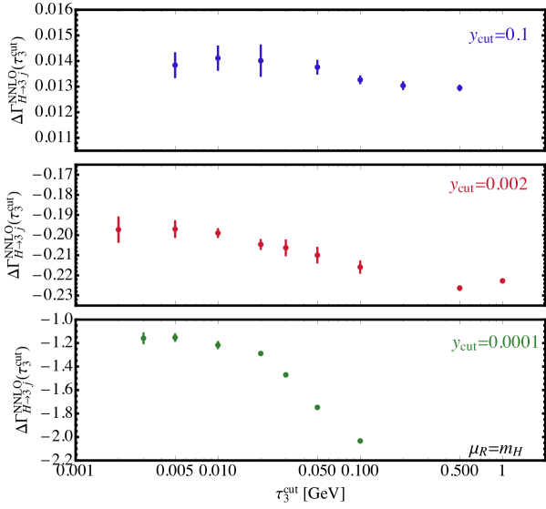
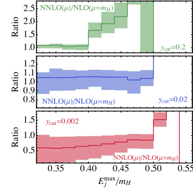
We first validate our calculation by studying the dependence of the NNLO coefficient on the unphysical slicing parameter . To do so we focus on three representative clustering options corresponding to , 0.002 and . These choices span the various regions of interest theoretically and experimentally. The value is within the perturbative regime, in which the higher-order corrections are expected to be small and agreement with future data should be good (assuming similarity to the NNLO calculations of jets GehrmannDeRidder:2008ug ; Weinzierl:2008iv ). The second choice corresponds to the region in which the three-jet rate peaks. Finally, the choice is around the region in which the NNLO three-jet rate turns negative and becomes unphysical (the need for resummation of large logarithms has set in long before this value is reached). The final choice is of particular relevance to this paper, since it corresponds to integrating the NNLO calculation with a very weak jet cut. Creating stable (and slicing-independent) results in this region allows us to test the code in phase-space configurations which correspond to two hard jets and one soft/collinear jet. Such configurations occur copiously in the calculation of at N3LO (where the soft jet is not required), and therefore establishing our code here is a prerequisite for this computation.
Our results for the three values are presented in Fig. 3. Asymptotic behavior is established in each region, with the dependence on missing power corrections having, as expected, a notable dependence on . For the larger choices the dependence on is rather mild, as the result for the largest value of is less than 10% different to that obtained in the asymptotic region (around GeV for and for ). The dependence on for is greater and asymptotic behavior is found for GeV. We therefore conclude that the power corrections are under control and that our code can be used to make phenomenological predictions. We note in passing that an LHC jet would be clustered using a -style algorithm and a jet with around GeV would loosely scale like GeV, so that the LHC case would look most like our results obtained when . In this region we have established that the power corrections are small and under control, and therefore our code could readily be applied to LHC processes such as . We leave this study to future work.
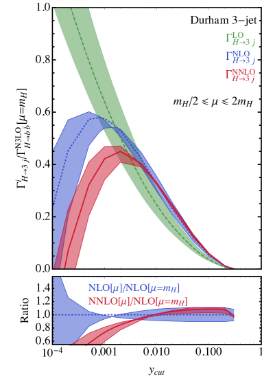
In Fig. 4 we show the exclusive three-jet rate at LO, NLO, and NNLO as a function of . We present results for the three-jet rate normalized to the N3LO inclusive rate Baikov:2005rw . In order to make each prediction we have set GeV, which is in the asymptotic region for nearly all of the phase space of interest. This choice is slightly too large for the smallest value of studied as discussed in the previous paragraph. However, the error on the coefficient for this choice is around 5%, which corresponds to a phenomenologically-acceptable correction on the total fractional jet rate. Our figure can be compared to similar results obtained for jets GehrmannDeRidder:2008ug ; Weinzierl:2008iv . The pattern is broadly the same, with a small positive correction in the large region (around 10%), which transitions to a decrease in the jet rate for . The three-jet rate is maximum at around and then turns over, becoming negative (and hence unphysical) in the region around . Along with the central scale choice of we also provide predictions for jet rates obtained with renormalization scales . In addition to the implicit dependence in the loop integral expansion, the predictions depend on also through the running of and at two- and three-loop order for our NLO and NNLO predictions respectively. We observe that the inclusion of the NNLO corrections substantially improves the overall scale dependence. This is especially true in the perturbative region specified by where we observe improvement of around a factor of two. For instance, at the overall scale dependence of the jet rate at NNLO is %, compared to % for the same jet cut at NLO. Finally, we note that in the perturbative region the scale variation bands provide a good estimate of the uncertainties due to the missing higher-order corrections, as the NNLO corrections lie within the NLO scale variation band. In this region we therefore expect the N3LO corrections to be within the NNLO band. On the other hand, in the region we observe that perturbation theory breaks down and, as expected, the scale variation bands no longer overlap. In this region the behavior of missing higher-order corrections cannot be predicted.
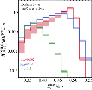
In Fig. 5 we turn our attention to differential distributions. We present the differential distribution for the energy component (rescaled by the Higgs mass) of the maximum-energy jet in three-jet events clustered with , , and . Comparing the three curves we observe that as decreases new phase space opens up near what would correspond to a two-jet LO topology, which occurs around . These configurations correspond to two nearly back-to-back jets with a soft/collinear third jet. In the perturbative region of the prediction is more physically sensible, the majority of jets having an energy close to with the most energetic jet peaking slightly higher than this value. For the cases = and the ratio of NNLO to NLO is reasonably flat and small (between ) until becomes large enough that there is no LO phase space configuration possible. In this region the NLO prediction is the first non-zero prediction and it is hence susceptible to large corrections at the next order. The scale variation mimics that of the total jet rate and is reasonably flat in the region in which the phase space is accessible to all of the contributing parton-level phase spaces. We have also computed differential distributions for smaller values of . They are not presented in Fig. 5 since, for such a small value of , the differential prediction is negative over a large range of phase space. We mention these predictions here simply to note that the code can produce stable distributions with small MC uncertainties even in this region, which is relevant to the N3LO results obtained in our companion paper.
5 Conclusions
In this paper we have presented the calculation of at NNLO. We have focused on the contributions in which the Higgs boson couples directly to bottom quarks. We have performed an independent computation of the two-loop amplitudes needed at this order and found agreement with a previous calculation in the literature. Additionally, we checked our result using the known IR factorization properties of QCD when the emitted gluon becomes soft or collinear to one of the fermions and found complete agreement with the predictions in both limits. We have presented the two-loop amplitudes for in full in the Appendix.
In order to regulate the IR divergences present at this order we used the -jettiness slicing technique to separate the calculation into two components. In the region of small we use SCET to construct an approximate form of the decay width. We used a computation of the 1-jettiness soft function, valid for arbitrary kinematics, coupled with the known jet functions and our computation of the hard function to construct the below-cut piece. The region corresponds to the NLO computation of the process, for which we calculated all of the needed helicity amplitudes using on-shell techniques of generalized unitarity for the one-loop pieces and BCFW recursion relations for the tree-level amplitudes.
We implemented our results into a Monte Carlo code, based upon the existing -jettiness slicing calculations of MCFM, and used it to produce differential distributions and jet rates for at NNLO using the Durham jet algorithm. Our calculation neglected top quark-induced contributions, which are phenomenologically relevant. By combing our results with the available EFT results we can produce predictions for relevant for the LHC and FCs which include both top and bottom Yukawa contributions. Additionally, by performing the appropriate kinematic crossings of our results we can compute at NNLO for LHC kinematics. We leave these applications to future studies.
One of the main goals of this paper was to investigate whether a stable (slicing-independent) Monte Carlo code could be constructed for very small jet cuts. We have established this by presenting rates and differential distributions for a variety of values of the jet-clustering variable . We are therefore able to effectively integrate out the jet at NNLO and use our results in a N3LO calculation. We pursue this approach in a companion paper to this article.
Acknowledgements.
We thank Ulrich Schubert for suggesting the coproduct method to simplify the 2dHPLs in the two-loop amplitudes and for helping with its implementation. We are grateful to Taushif Ahmed for clarifying the results of Ref. Ahmed:2014pka . CW and RM are supported by a National Science Foundation CAREER award number PHY-1652066. Support provided by the Center for Computational Research at the University at Buffalo.Note added
A previous version of this manuscript, submitted to the arXiv, incorrectly claimed a disagreement with the existing two-loop calculation presented in Ref. Ahmed:2014pka . This was due to a misinterpretation on our part of the results of Ref. Ahmed:2014pka . Specifically, in two of the coefficients in Ref. Ahmed:2014pka the Mandelstam invariants and are retained (the remaining coefficients are functions of the variables and only), whereas our results are constructed in terms of and only. Our notation is different from Ref. Ahmed:2014pka () and the residual and dependence in the two coefficients was incorrectly evaluated in our initial comparison. Once this is altered accordingly our results are in perfect agreement.
Appendix A Formulae for renormalization and IR subtraction
The renormalization coefficients of Eqs. (18) and (19) are defined as
| (35) | ||||
| (36) | ||||
| (37) | ||||
| (38) |
with
| (39) | ||||
| (40) |
and , , .
The subtraction operators for generic QCD processes can be found in Ref. Catani:1998bh . For completeness, we show here the explicit expressions for the subtraction operators in CDR for the process :
| (41) | ||||
| (42) |
where
| (43) | ||||
| (44) |
with
| (45) | ||||
| (46) |
Appendix B One-loop and two-loop coefficients for
We present the explicit results for the coefficients and of Eq. (26) as series in . The results for the one-loop and two-loop coefficients are also available in a supplementary Mathematica-readable file attached to this paper. At tree level the coefficients are
| (52) |
At one loop the coefficients read:
| (53) | ||||
| (54) | ||||
| (55) | ||||
| (56) |
At two loops:
| (57) | ||||
| (58) | ||||
| (59) | ||||
| (60) | ||||
| (61) | ||||
| (62) |
where
| (63) | ||||
| (64) | ||||
| (65) | ||||
| (66) | ||||
| (67) | ||||
| (68) |
and
| (69) | ||||
| (70) | ||||
| (71) | ||||
| (72) | ||||
| (73) | ||||
| (74) |
Appendix C Formulae for soft and collinear limits
We list the unrenormalized matrix elements that are needed for the soft and collinear limit checks of the two-loop amplitude. The matrix elements in CDR read:
| (75) | ||||
| (76) | ||||
| (77) |
where is taken from Eq. (2.24) of Ref. Gehrmann:2014vha and .
The soft currents in Eq. (32) are defined as
| (78) | ||||
| (79) | ||||
| (80) |
where and have been adapted from Eqs. (12), (13), and (26) of Ref. Catani:2000pi , while is taken from Eq. (11) of Ref. Li:2013lsa .
The collinear functions in Eq. (33) are
| (81) | ||||
| (82) | ||||
| (83) |
The tree-level splitting functions in CDR are (see Eqs. (4.17) and (4.18) of Ref. Badger:2004uk ):
| (84) | ||||
| (85) |
At one loop, the splitting functions in CDR are (see Eqs. (4.21) and (4.22) of Ref. Badger:2004uk ):
| (86) | ||||
| (87) |
with
| (88) | ||||
| (89) |
The two-loop splitting functions in CDR are (see Eqs. (3.7)(3.14) and (4.24)(4.25) of Ref. Badger:2004uk ):
| (90) |
where
| (91) |
with and as defined in Appendix A. Finally, the functions and correspond to Eqs. (4.24) and (4.25) of Ref. Badger:2004uk respectively with the replacement .
References
- (1) ATLAS Collaboration, G. Aad et. al., Observation of a new particle in the search for the Standard Model Higgs boson with the ATLAS detector at the LHC, Phys. Lett. B716 (2012) 1–29 [1207.7214].
- (2) CMS Collaboration, S. Chatrchyan et. al., Observation of a new boson at a mass of 125 GeV with the CMS experiment at the LHC, Phys. Lett. B716 (2012) 30–61 [1207.7235].
- (3) H. Baer, T. Barklow, K. Fujii, Y. Gao, A. Hoang, S. Kanemura, J. List, H. E. Logan, A. Nomerotski, M. Perelstein et. al., The International Linear Collider Technical Design Report - Volume 2: Physics, 1306.6352.
- (4) TLEP Design Study Working Group Collaboration, M. Bicer et. al., First Look at the Physics Case of TLEP, JHEP 01 (2014) 164 [1308.6176].
- (5) FCC Collaboration, A. Abada et. al., FCC-ee: The Lepton Collider, . [Eur. Phys. J. ST228,no.2,261(2019)].
- (6) ATLAS Collaboration, M. Aaboud et. al., Observation of decays and production with the ATLAS detector, Phys. Lett. B786 (2018) 59–86 [1808.08238].
- (7) CMS Collaboration, A. M. Sirunyan et. al., Observation of Higgs boson decay to bottom quarks, Phys. Rev. Lett. 121 (2018), no. 12 121801 [1808.08242].
- (8) CMS Collaboration, A. M. Sirunyan et. al., Inclusive search for a highly boosted Higgs boson decaying to a bottom quark-antiquark pair, Phys. Rev. Lett. 120 (2018), no. 7 071802 [1709.05543].
- (9) C. Anastasiou, C. Duhr, F. Dulat, F. Herzog and B. Mistlberger, Higgs Boson Gluon-Fusion Production in QCD at Three Loops, Phys. Rev. Lett. 114 (2015) 212001 [1503.06056].
- (10) C. Anastasiou, C. Duhr, F. Dulat, E. Furlan, T. Gehrmann, F. Herzog, A. Lazopoulos and B. Mistlberger, High precision determination of the gluon fusion Higgs boson cross-section at the LHC, JHEP 05 (2016) 058 [1602.00695].
- (11) S. Catani and M. Grazzini, An NNLO subtraction formalism in hadron collisions and its application to Higgs boson production at the LHC, Phys. Rev. Lett. 98 (2007) 222002 [hep-ph/0703012].
- (12) L. Cieri, X. Chen, T. Gehrmann, E. W. N. Glover and A. Huss, Higgs boson production at the LHC using the subtraction formalism at N3LO QCD, JHEP 02 (2019) 096 [1807.11501].
- (13) F. Dulat, B. Mistlberger and A. Pelloni, Differential Higgs production at N3LO beyond threshold, JHEP 01 (2018) 145 [1710.03016].
- (14) F. Dulat, B. Mistlberger and A. Pelloni, Precision predictions at N3LO for the Higgs boson rapidity distribution at the LHC, Phys. Rev. D99 (2019), no. 3 034004 [1810.09462].
- (15) R. Boughezal, F. Caola, K. Melnikov, F. Petriello and M. Schulze, Higgs boson production in association with a jet at next-to-next-to-leading order in perturbative QCD, JHEP 06 (2013) 072 [1302.6216].
- (16) X. Chen, T. Gehrmann, E. W. N. Glover and M. Jaquier, Precise QCD predictions for the production of Higgs + jet final states, Phys. Lett. B740 (2015) 147–150 [1408.5325].
- (17) J. M. Campbell, R. K. Ellis and G. Zanderighi, Next-to-Leading order Higgs + 2 jet production via gluon fusion, JHEP 10 (2006) 028 [hep-ph/0608194].
- (18) G. Cullen, H. van Deurzen, N. Greiner, G. Luisoni, P. Mastrolia, E. Mirabella, G. Ossola, T. Peraro and F. Tramontano, Next-to-Leading-Order QCD Corrections to Higgs Boson Production Plus Three Jets in Gluon Fusion, Phys. Rev. Lett. 111 (2013), no. 13 131801 [1307.4737].
- (19) T. Gehrmann, M. Jaquier, E. W. N. Glover and A. Koukoutsakis, Two-Loop QCD Corrections to the Helicity Amplitudes for 3 partons, JHEP 02 (2012) 056 [1112.3554].
- (20) E. Braaten and J. P. Leveille, Higgs Boson Decay and the Running Mass, Phys. Rev. D22 (1980) 715.
- (21) C. Anastasiou, F. Herzog and A. Lazopoulos, The fully differential decay rate of a Higgs boson to bottom-quarks at NNLO in QCD, JHEP 03 (2012) 035 [1110.2368].
- (22) V. Del Duca, C. Duhr, G. Somogyi, F. Tramontano and Z. Trócsányi, Higgs boson decay into b-quarks at NNLO accuracy, JHEP 04 (2015) 036 [1501.07226].
- (23) W. Bernreuther, L. Chen and Z.-G. Si, Differential decay rates of CP-even and CP-odd Higgs bosons to top and bottom quarks at NNLO QCD, JHEP 07 (2018) 159 [1805.06658].
- (24) P. A. Baikov, K. G. Chetyrkin and J. H. Kuhn, Scalar correlator at O(alpha(s)**4), Higgs decay into b-quarks and bounds on the light quark masses, Phys. Rev. Lett. 96 (2006) 012003 [hep-ph/0511063].
- (25) T. Ahmed, M. Mahakhud, P. Mathews, N. Rana and V. Ravindran, Two-loop QCD corrections to Higgs amplitude, JHEP 08 (2014) 075 [1405.2324].
- (26) R. Mondini, M. Schiavi and C. Williams, N3LO predictions for the decay of the Higgs boson to bottom quarks, 1904.08960.
- (27) K. G. Chetyrkin, Correlator of the quark scalar currents and Gamma(tot) (H —> hadrons) at O (alpha-s**3) in pQCD, Phys. Lett. B390 (1997) 309–317 [hep-ph/9608318].
- (28) T. Gehrmann and D. Kara, The form factor to three loops in QCD, JHEP 09 (2014) 174 [1407.8114].
- (29) A. Primo, G. Sasso, G. Somogyi and F. Tramontano, Exact Top Yukawa corrections to Higgs boson decay into bottom quarks, 1812.07811.
- (30) J. Gaunt, M. Stahlhofen, F. J. Tackmann and J. R. Walsh, N-jettiness Subtractions for NNLO QCD Calculations, JHEP 09 (2015) 058 [1505.04794].
- (31) R. Boughezal, C. Focke, X. Liu and F. Petriello, -boson production in association with a jet at next-to-next-to-leading order in perturbative QCD, Phys. Rev. Lett. 115 (2015), no. 6 062002 [1504.02131].
- (32) I. W. Stewart, F. J. Tackmann and W. J. Waalewijn, N-Jettiness: An Inclusive Event Shape to Veto Jets, Phys. Rev. Lett. 105 (2010) 092002 [1004.2489].
- (33) N. Brown and W. J. Stirling, Jet cross-sections at leading double logarithm in e+ e- annihilation, Phys. Lett. B252 (1990) 657–662.
- (34) S. Catani, Y. L. Dokshitzer, M. Olsson, G. Turnock and B. R. Webber, New clustering algorithm for multi - jet cross-sections in e+ e- annihilation, Phys. Lett. B269 (1991) 432–438.
- (35) I. W. Stewart, F. J. Tackmann and W. J. Waalewijn, Factorization at the LHC: From PDFs to Initial State Jets, Phys. Rev. D81 (2010) 094035 [0910.0467].
- (36) T. Becher and M. Neubert, Toward a NNLO calculation of the anti-B —> X(s) gamma decay rate with a cut on photon energy. II. Two-loop result for the jet function, Phys. Lett. B637 (2006) 251–259 [hep-ph/0603140].
- (37) J. M. Campbell, R. K. Ellis, R. Mondini and C. Williams, The NNLO QCD soft function for 1-jettiness, Eur. Phys. J. C78 (2018), no. 3 234 [1711.09984].
- (38) R. Boughezal, X. Liu and F. Petriello, -jettiness soft function at next-to-next-to-leading order, Phys. Rev. D91 (2015), no. 9 094035 [1504.02540].
- (39) Z. Bern, L. J. Dixon, D. C. Dunbar and D. A. Kosower, One loop n point gauge theory amplitudes, unitarity and collinear limits, Nucl. Phys. B425 (1994) 217–260 [hep-ph/9403226].
- (40) R. Britto, F. Cachazo and B. Feng, Generalized unitarity and one-loop amplitudes in N=4 super-Yang-Mills, Nucl. Phys. B725 (2005) 275–305 [hep-th/0412103].
- (41) D. Forde, Direct extraction of one-loop integral coefficients, Phys. Rev. D75 (2007) 125019 [0704.1835].
- (42) P. Mastrolia, Double-Cut of Scattering Amplitudes and Stokes’ Theorem, Phys. Lett. B678 (2009) 246–249 [0905.2909].
- (43) S. D. Badger, Direct Extraction Of One Loop Rational Terms, JHEP 01 (2009) 049 [0806.4600].
- (44) R. K. Ellis, W. T. Giele, Z. Kunszt and K. Melnikov, Masses, fermions and generalized -dimensional unitarity, Nucl. Phys. B822 (2009) 270–282 [0806.3467].
- (45) S. Badger, E. W. Nigel Glover, P. Mastrolia and C. Williams, One-loop Higgs plus four gluon amplitudes: Full analytic results, JHEP 01 (2010) 036 [0909.4475].
- (46) R. Britto, F. Cachazo, B. Feng and E. Witten, Direct proof of tree-level recursion relation in Yang-Mills theory, Phys. Rev. Lett. 94 (2005) 181602 [hep-th/0501052].
- (47) J. Alwall, M. Herquet, F. Maltoni, O. Mattelaer and T. Stelzer, MadGraph 5 : Going Beyond, JHEP 06 (2011) 128 [1106.0522].
- (48) S. Catani and M. H. Seymour, A General algorithm for calculating jet cross-sections in NLO QCD, Nucl. Phys. B485 (1997) 291–419 [hep-ph/9605323]. [Erratum: Nucl. Phys.B510,503(1998)].
- (49) T. Becher, G. Bell, C. Lorentzen and S. Marti, Transverse-momentum spectra of electroweak bosons near threshold at NNLO, JHEP 02 (2014) 004 [1309.3245].
- (50) T. Hahn, Generating Feynman diagrams and amplitudes with FeynArts 3, Comput. Phys. Commun. 140 (2001) 418–431 [hep-ph/0012260].
- (51) P. Maierhöfer, J. Usovitsch and P. Uwer, Kira—A Feynman integral reduction program, Comput. Phys. Commun. 230 (2018) 99–112 [1705.05610].
- (52) R. N. Lee, LiteRed 1.4: a powerful tool for reduction of multiloop integrals, J. Phys. Conf. Ser. 523 (2014) 012059 [1310.1145].
- (53) L. W. Garland, T. Gehrmann, E. W. N. Glover, A. Koukoutsakis and E. Remiddi, The Two loop QCD matrix element for e+ e- —> 3 jets, Nucl. Phys. B627 (2002) 107–188 [hep-ph/0112081].
- (54) E. Remiddi and J. A. M. Vermaseren, Harmonic polylogarithms, Int. J. Mod. Phys. A15 (2000) 725–754 [hep-ph/9905237].
- (55) T. Gehrmann and E. Remiddi, Two loop master integrals for gamma* —> 3 jets: The Planar topologies, Nucl. Phys. B601 (2001) 248–286 [hep-ph/0008287].
- (56) T. Gehrmann and E. Remiddi, Two loop master integrals for gamma* –> 3 jets: The Nonplanar topologies, Nucl. Phys. B601 (2001) 287–317 [hep-ph/0101124].
- (57) C. Duhr, Mathematical aspects of scattering amplitudes, in Proceedings, Theoretical Advanced Study Institute in Elementary Particle Physics: Journeys Through the Precision Frontier: Amplitudes for Colliders (TASI 2014): Boulder, Colorado, June 2-27, 2014, pp. 419–476, 2015. 1411.7538.
- (58) S. Catani, The Singular behavior of QCD amplitudes at two loop order, Phys. Lett. B427 (1998) 161–171 [hep-ph/9802439].
- (59) Y. Li and H. X. Zhu, Single soft gluon emission at two loops, JHEP 11 (2013) 080 [1309.4391].
- (60) S. D. Badger and E. W. N. Glover, Two loop splitting functions in QCD, JHEP 07 (2004) 040 [hep-ph/0405236].
- (61) C. Duhr, T. Gehrmann and M. Jaquier, Two-loop splitting amplitudes and the single-real contribution to inclusive Higgs production at N3LO, JHEP 02 (2015) 077 [1411.3587].
- (62) J. M. Campbell and R. K. Ellis, An Update on vector boson pair production at hadron colliders, Phys. Rev. D60 (1999) 113006 [hep-ph/9905386].
- (63) J. M. Campbell, R. K. Ellis and C. Williams, Vector boson pair production at the LHC, JHEP 07 (2011) 018 [1105.0020].
- (64) J. M. Campbell, R. K. Ellis and W. T. Giele, A Multi-Threaded Version of MCFM, Eur. Phys. J. C75 (2015), no. 6 246 [1503.06182].
- (65) R. Boughezal, J. M. Campbell, R. K. Ellis, C. Focke, W. Giele, X. Liu, F. Petriello and C. Williams, Color singlet production at NNLO in MCFM, Eur. Phys. J. C77 (2017), no. 1 7 [1605.08011].
- (66) A. Gehrmann-De Ridder, T. Gehrmann, E. W. N. Glover and G. Heinrich, Jet rates in electron-positron annihilation at O(alpha(s)**3) in QCD, Phys. Rev. Lett. 100 (2008) 172001 [0802.0813].
- (67) S. Weinzierl, NNLO corrections to 3-jet observables in electron-positron annihilation, Phys. Rev. Lett. 101 (2008) 162001 [0807.3241].
- (68) S. Catani and M. Grazzini, The soft gluon current at one loop order, Nucl. Phys. B591 (2000) 435–454 [hep-ph/0007142].