Class Specific or Shared? A Cascaded Dictionary Learning Framework for Image Classification

Abstract

Dictionary learning methods can be split into: i) class specific dictionary learning ii) class shared dictionary learning. The difference between the two categories is how to use discriminative information. With the first category, samples of different classes are mapped into different subspaces, which leads to some redundancy with the class specific base vectors. While for the second category, the samples in each specific class can not be described accurately. In this paper, we first propose a novel class shared dictionary learning method named label embedded dictionary learning (LEDL). It is the improvement based on LCKSVD, which is easier to find out the optimal solution. Then we propose a novel framework named cascaded dictionary learning framework (CDLF) to combine the specific dictionary learning with shared dictionary learning to describe the feature to boost the performance of classification sufficiently. Extensive experimental results on six benchmark datasets illustrate that our methods are capable of achieving superior performance compared to several state-of-art classification algorithms.

1 Introduction

In recent years, image classification has been a classical issue in pattern recognition. With advancement in theory, many image classification methods have been proposed Wright et al. (2009); Liu et al. (2019); Zhang et al. (2011); Yang et al. (2009); Liu et al. (2016, 2017); Aharon et al. (2006); Zhang and Li (2010); Jiang et al. (2013); Chan et al. (2015); He et al. (2016). In these methods, there is one category that contributes a lot for image classification which is the dictionary learning (DL) based method. DL is a generative model of which the concept was firstly proposed by Mallat et al. Mallat and Zhang (1993). A few years later, Olshausen et al. Olshausen and Field (1996, 1997) proposed an application of DL on natural images and then it has been widely used in many fields such as image denoising Li et al. (2018, 2012), image superresolution Gao et al. (2018); Jiang et al. (2019) and image classification Li et al. (2019); Lin et al. (2018). According to different ways of utilizing the discriminative information, DL methods can be split into two categories: i) class specific dictionary learning ii) class shared dictionary learning.

Class specific dictionary learning method utilizes the discriminative information by adding discrimination ability into a dictionary. The learned dictionary is for each class. This category can gain the representative feature information of a class. The feature information that most of the class’s samples have is focused on, while only a few samples of the class have is ignored to some extent. That is to say, the learned dictionary has higher weight on the feature information which samples close to the distribution center, and lower weight on the feature information that samples off the center. With this method, some abnormal sample points are ignored so that the learned dictionary’s robustness can be improved. There are many classical class specific dictionary learning algorithms that have been reported in recent years. For example, fisher discrimination dictionary learning (FDDL) Yang et al. (2011) uses the fisher discrimination criterion to learn a structured dictionary for pattern classification. In this method, each sub-dictionary can well reconstruct the signals from the same class. Different from FDDL, projective dictionary pair learning (DPL) Gu et al. (2014) and sevral following works such as robust adaptive dictionary pair learning (RA-DPL) Sun et al. (2020), twin-projective latent dictionary pairs learning (TP-DPL) Zhang et al. (2019c) extend the regular dictionary learning to dictionary pair learning. This kind of approach achieves the goal of signal representation and discrimination by jointly learning a synthesis dictionary and an analysis dictionary. Moreover, discriminative Bayesian dictionary learning (DBDL) Akhtar et al. (2016) and joint embedding and dictionary learning framework (JEDL) Zhang et al. (2016) are two effective methods based class specific DL for classification. Specifically, DBDL complete classification task by approaching a non-parametric Bayesian perspective and JEDL do it according to deliver a linear sparse codes auto-extractor and a multi-class classifier by simultaneously minimizing the sparse reconstruction, discriminative sparse-code, code approximation, and classification errors.

Due that the learned dictionary is for each class, the training samples of each class are mapped into a separate subspace. First, different dictionaries can be regarded as different subspaces, which ensure that the salient characteristics of each category are elegantly described ($\ell_{1}$ norm constraint would generate the salient characteristics), and the discriminative information among different categories is obtained obviously (for each category, most of the learned atoms have their category characteristics and only a few will overlap with other categories’ atoms). Second, each atom of dictionaries is $\ell_{2}$ normalized to guarantee that all the atoms are distributed on a hyper-surface. And thus, the projection of the image features is under the same scale. Third, although different dictionaries can be regarded as different subspaces, these dictionaries are not unrelated. For example, for the face dataset, different categories usually have the same characteristics (e.g., similar facial structure). When learning the dictionaries, the atoms would have some intersections or overlaps, which ensure that different categories of projections are comparable.

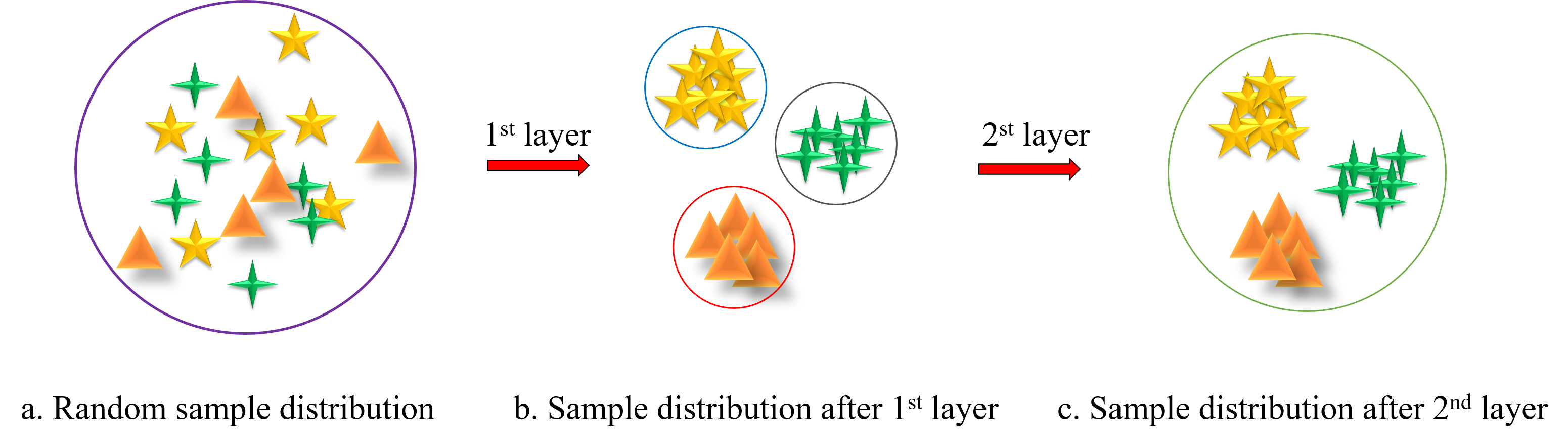
Figure 1: Illustration of the variation of sample distribution. Different circles represent different subspaces.

For class shared dictionary learning method, the discriminative information is directly embedded into the objective function to learn a dictionary for all classes. With this method, the training samples from all classes are mapped into one subspace. Hence, the representative feature information of all classes can be adopted. In recent years, many class shared dictionary learning methods have been proposed. For instance, label consistent K-SVD (LC-KSVD) Jiang et al. (2013) proposed a new method to use a discriminative dictionary for sparse coding. In robust flexible discriminative dictionary learning (RFDDL) Zhang et al. (2019b), the labels are utilized flexibly to enhance the robust property to sparse errors and encoding the locality, reconstruction error and label consistency more accurately. And the joint robust factorization and projective dictionary learning (J-RFDL) Ren et al. (2020) discovered the hybrid salient low-rank and sparse representation in a factorized compressed space and use it improve the data representations. All of the above-mentioned methods which are based on class shared dictionary learning approaches to update the dictionary, have got an outstanding performance on classification tasks. However, it can not describe the samples in each specific class accurately so that the detailed features between samples in one class can not be found easily.

In comparison to class specific dictionary learning and class shared dictionary learning, it is clear that the two methods have complementary advantages. It would help to obtain a significant boost in classification accuracy if the advantages of the two dictionary learning methods can be appropriately combined. In this paper, we first propose a novel class shared dictionary learning algorithm named label embedded dictionary learning (LEDL). This method introduces the $\ell_{1}$-norm regularization term to replace the $\ell_{0}$-norm regularization of LC-KSVD. In LC-KSVD, $\ell_{0}$-norm based sparse regularization term leads to the NP-hard problem. Even though many classical greedy methods such as orthogonal matching pursuit (OMP) Tropp and Gilbert (2007) have solved this problem to some extent, it is usually to find the suboptimum sparse solution instead of the optimal sparse solution. In addition, the greedy method solves the global optimal problems by finding basis vectors in order of reconstruction errors from small to large until $T$ (the sparsity constraint factor) times. Thus, the initialized values are crucial. To this end, there are still many restrictions by using $\ell_{0}$-norm based sparse constraint. While our proposed LEDL is helpful to solve this problem. Moreover, compared with some dictionary learning methods without $\ell_{0}/\ell_{0}$-norm regularization term, such as robust label embedding projective dictionary learning (LE-PDL) Jiang et al. (2017) and scalable locality-constrained projective dictionary learning (LC-PDL) Zhang et al. (2019a), our proposed methods are more general. Despite the fact that these methods have achieved good performance, they may lead to some singular values which come from the non-full rank matrices in some datasets. After that, we propose a novel framework named cascaded dictionary learning framework (CDLF) to combine a class specific dictionary learning method with a class shared dictionary learning method together.

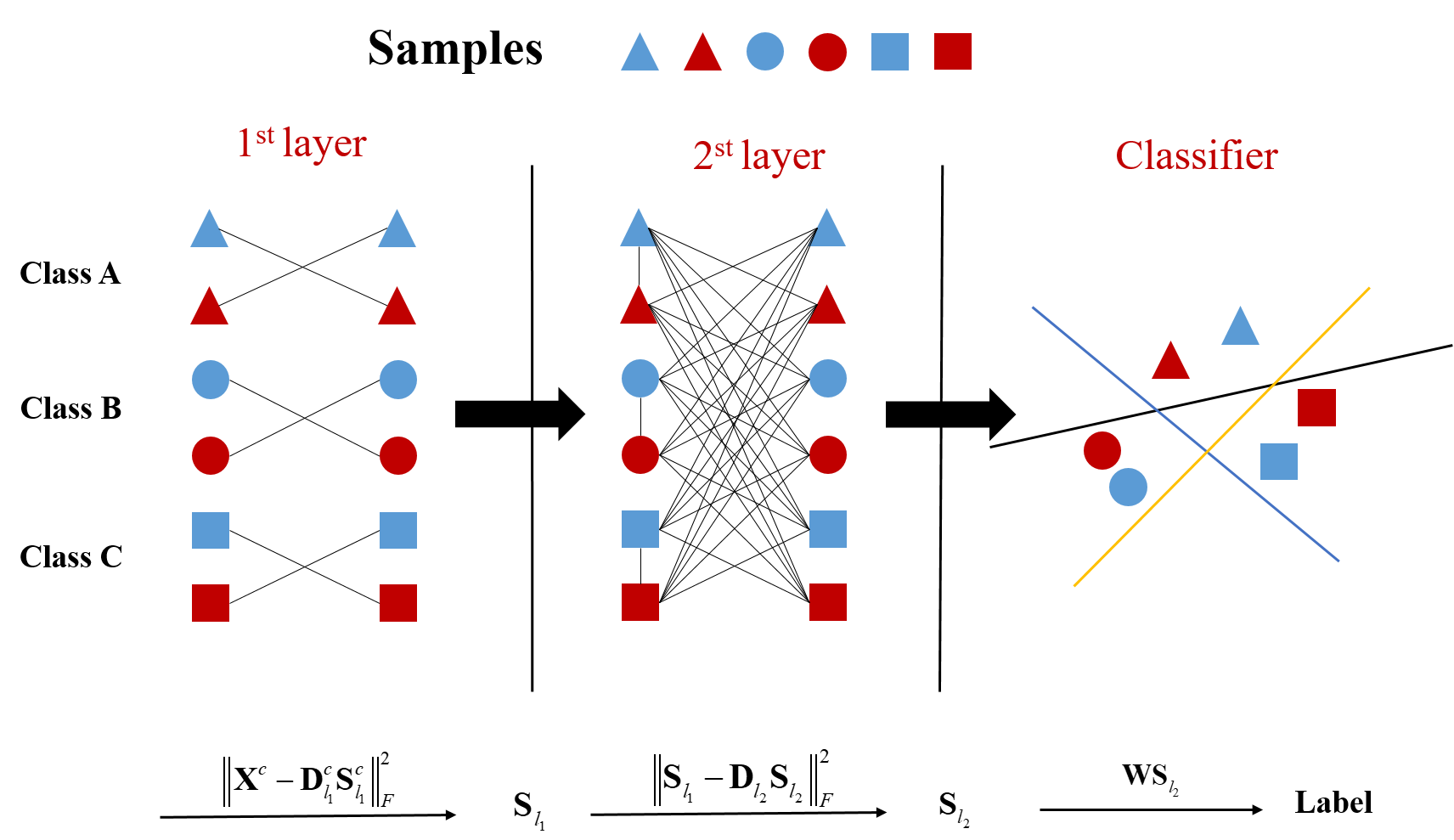
Figure 2: Illustration of the cascaded dictionary learning framework (CDLF). In the first layer, accurate subspaces are created for each class by class specific dictionary method. Therefore the samples from the same class are clustered together. In the second layer, the label embeded dictionary learning method establishes a discriminative subspace for all classes. $\bf{X}$ represents the sample matrix, $\bf{D}$, $\bf{{S}}$ are dictionary matrix and sparse codes matrix, respectively. $\bf{{W}}$ represents the learned classifier.

Our framework contains two layers. Specifically, the first layer consists of the class specific dictionary learning for sparse representation (CSDL-SRC) Liu et al. (2016) method, it is used to extract the crucial feature information of a class to wipe off singular points and improve robustness. The second layer is composed of LEDL which pulled the feature information belongs to different subspaces back into the same subspace to obtain the relationship among different classes. To be attention, different from the recent work CDPL-Net Zhang et al. (2020) which is a deep dictionary learning network, our proposed framework is a whole structure that can replace the dictionary pair learning layer of the network.

In addition, the feature after the first layer has been a better representation as to the reason that the objective function introduced the discriminative information and map them into different subspaces for the classifier which trained from the second layer. Thus, we can regard the first layer as a helpful tool to obtain excellent features. It does not work if we set the class shared dictionary learning method as the first layer and the class specific dictionary learning as the second layer. Figure 1 shows the variation of sample distribution. Figure 1 $a$ shows the random distribution samples belong to three classes; Figure 1 $b$ shows that the samples belong to the same class are clustered while the samples of three classes are in different subspaces; Figure 1 $c$ shows that the samples in different subspaces are pulled back into the same subspace. A schematic description of our proposed CDLF is given in Figure 2.

We adopt the alternating direction method of multipliers (ADMM) Boyd et al. (2011) algorithm and blockwise coordinate descent (BCD) Liu et al. (2014) algorithm to optimize CDLF. The contributions of this work are four-fold:

• We propose a novel class shared dictionary learning method named label embedded dictionary learning (LEDL) that introduces the $\ell_{1}$-norm regularization term as the sparse constraint. The $\ell_{1}$-norm sparse constraint can easily find the optimal sparse solution.

• We propose a novel dictionary learning framework named cascaded dictionary learning framework (CDLF), which is the first time we combine the class specific and shared dictionary learning. More specifically, discriminative information is used in different ways to fully describe the feature while completely maintain the discriminative information. The CDLF can be considered as the extension of conventional dictionary learning algorithms.

• We propose to utilize the alternating direction method of multipliers (ADMM) Boyd et al. (2011) algorithm and blockwise coordinate descent (BCD) Liu et al. (2014) algorithm to optimize each layer of a dictionary learning task.

• We evaluate the proposed LEDL and CDLF methods on six benchmark datasets, and the achieved superior performance verifies the effectiveness of our proposed methods.

We organize the rest of the paper as follows. Section  2 introduces two related algorithms, which are CSDL-SRC and LC-KSVD. Section 3 presents CDLF for image classification. section 4 shows some experiments and analyses. Finally, we conclude this paper in Section 5.

2 Related Work

In this section, we overview two related dictionary learning methods, including class specific dictionary learning for sparse representation (CSDL-SRC) and label consistent K-SVD (LC-KSVD).

2.1 Class specific dictionary learning for sparse representation (CSDL-SRC)

Liu et al. Liu et al. (2016) proposed CSDL-SRC to reduce the high residual error and instability of SRC. The authors consider the weight of each sample feature when generating the dictionary. Assume that ${\bf{X}}=\left[{{{\bf{X}}^{1}},{{\bf{X}}^{2}},\cdots,{{\bf{X}}^{C}}}\right]\in{{\mathbb{R}}^{d\times N}}$ is the training sample matrix, where $d$ represents the dimensions of the sample features, $N$ and $C$ are the number of training samples and the class number of training samples, respectively. The $c_{th}$ class of training sample matrix is denoted as ${{\bf{X}}^{c}}\in{{\mathbb{R}}^{d\times N^{c}}}$, where $c=1,2,\cdots,C$ and $N^{c}$ is the $c_{th}$ class of $N$($N=\sum\limits_{c=1}^{C}{{N^{c}}}$). Liu et al. build a weight coefficient matrix ${{\bf{P}}^{c}}\in{{\mathbb{R}}^{{N^{c}}\times{K^{c}}}}$ for ${{\bf{X}}^{c}}$, where ${K}$ is the dictionary size of CSDL-SRC and ${K^{c}}$ is the $c_{th}$ class of $K$ (${K}=\sum\limits_{c=1}^{C}{K^{c}}$). The objective function of CSDL-SRC is as follows:

$$\scriptsize\begin{split}<{{\bf{P}}^{c}},{{\bf{U}}^{c}}>&=\mathop{\arg\min}\limits_{{{\bf{P}}^{c}},{{\bf{U}}^{c}}}\left\|{{{\bf{X}}^{c}}-{{\bf{X}}^{c}}{{\bf{P}}^{c}}{{\bf{U}}^{c}}}\right\|_{F}^{2}+2\zeta{\left\|{{{\bf{U}}^{c}}}\right\|_{\ell_{1}}}\\ &s.t.\left\|{\bf{X}^{c}{\bf{P}}_{\bullet k}^{c}}\right\|_{2}^{2}\leq 1\;\;\;(k=1,2,\cdots,{K})\end{split}$$ (1)

where ${{\bf{U}}^{c}}\in{{\mathbb{R}}^{{K^{c}}\times N^{c}}}$ is the sparse codes of ${\bf{X}^{c}}$, the $\ell_{1}$-norm regularization term is utilized to enforce the sparsity, $\zeta$ is the regularization parameter to control the tradeoff between fitting goodness and sparseness. The ${{\left(\bullet\right)}_{\bullet k}}$ denote the $k_{th}$ column vector of matrix ${\left(\bullet\right)}$.

2.2 Label consistent K-SVD (LC-KSVD)

Jiang et al. Jiang et al. (2013) proposed LC-KSVD to combine the discriminative sparse codes error with the reconstruction error and the classification error to form a unified objective function which is defined as follows:

$$\scriptsize\begin{split}<{\bf{B}},{\bf{W}},{\bf{A}},{\bf{V}}>&=\mathop{\arg\min}\limits_{{\bf{B}},{\bf{W}},{\bf{A}},{\bf{V}}}\left\|{{\bf{X}}-{\bf{BV}}}\right\|_{F}^{2}+\lambda\left\|{{\bf{H}}-{\bf{WV}}}\right\|_{F}^{2}+\omega\left\|{{\bf{Q}}-{\bf{AV}}}\right\|_{F}^{2}\\ {\kern 12.0pt}&s.t.{\kern 3.0pt}{\left\|{{{\bf{v}}_{i}}}\right\|_{0}}<T{\kern 6.0pt}\left({i=1,2\cdots,N}\right)\end{split}$$ (2)

where $T$ is the sparsity constraint factor, ${\bf{B}}\in{{\mathbb{R}}^{d\times K}}$ is the dictionary matrix of $\bf{X}$, ${\bf{V}}\in{{\mathbb{R}}^{K\times d}}$ is the sparse codes matrix of ${\bf{X}}$. ${\bf{W}}\in{{\mathbb{R}}^{C\times K}}$ is a classifier matrix learned from the given label matrix ${\bf{H}}\in{{\mathbb{R}}^{C\times N}}$. We hope ${\bf{W}}$ can return the most probable class this sample belongs to. ${\bf{Q}}\in{{\mathbb{R}}^{K\times N}}$ represents the discriminative sparse codes matrix and ${\bf{A}}=\left[{{{\bf{a}}_{1}},{{\bf{a}}_{2}},\cdots,{{\bf{a}}_{K_{2}}}}\right]\in{{\mathbb{R}}^{K_{2}\times K_{2}}}$ is a linear transformation matrix relys on ${\bf{Q}}$. $\lambda$ and $\omega$ are the regularization parameters balancing the discriminative sparse codes errors and the classification contribution to the overall objective function, respectively.

3 Methodology

In this section, we elaborate on the construction of a cascaded dictionary learning framework (CDLF). Specifically, in subsection 3.1, we introduce the label embedded dictionary learning method. In subsection 3.2, we propose the cascaded method of the first layer and the second layer. In subsection 3.3, we give the optimization method of objective function.

3.1 Label embedded dictionary learning (LEDL)

This subsection proposes a novel dictionary learning method named label embedded dictionary learning (LEDL) for image classification. LEDL is an improvement of LC-KSVD, which introducing the $\ell_{1}$-norm regularization term to replace the $\ell_{0}$-norm regularization of LC-KSVD. Thus, we can freely select the basis vectors for linear fitting to obtain an optimal sparse solution instead of a suboptimal solution.

The objection function is as follows and the $\varepsilon$ is the regularization parameter:

$$\scriptsize\begin{split}<{\bf{B}},{\bf{W}},{\bf{A}},{\bf{V}}>=&\mathop{\arg\min}\limits_{{\bf{B}},{\bf{W}},{\bf{A}},{\bf{V}}}\left\|{{\bf{X}}-{\bf{BV}}}\right\|_{F}^{2}+\lambda\left\|{{\bf{H}}-{\bf{WV}}}\right\|_{F}^{2}\\ &+\omega\left\|{{\bf{Q}}-{\bf{AV}}}\right\|_{F}^{2}+2\varepsilon{\left\|{\bf{V}}\right\|_{\ell_{1}}}\\ {\rm{s}}.t.{\kern 4.0pt}\left\|{{{\bf{B}}_{\bullet k}}}\right\|_{2}^{2}\leq 1,{\kern 1.0pt}{\kern 1.0pt}&\left\|{{{\bf{W}}_{\bullet k}}}\right\|_{2}^{2}\leq 1,{\kern 1.0pt}\left\|{{{\bf{A}}_{\bullet k}}}\right\|_{2}^{2}\leq 1{\kern 3.0pt}\left({k=1,2,\cdots K}\right)\end{split}$$ (3)

Where the definitions of $\bf{W}$, $\bf{W}$, $\bf{A}$, $\bf{V}$ in Equation 3 are same with the ones in Equation 2. Consider the optimization problem (3) is not jointly convex in both ${\bf{V}}$, ${\bf{B}}$, ${\bf{W}}$ and ${\bf{A}}$, it is separately convex in either ${\bf{V}}$ (with ${\bf{B}}$, ${\bf{W}}$, ${\bf{A}}$ fixed), ${\bf{B}}$ (with ${\bf{V}}$, ${\bf{W}}$, ${\bf{A}}$ fixed), ${\bf{W}}$ (with ${\bf{V}}$, ${\bf{B}}$, ${\bf{A}}$ fixed) or ${\bf{A}}$ (with ${\bf{V}}$, ${\bf{B}}$, ${\bf{W}}$ fixed). Thus, we recognised the optimization as four optimization subproblems. Futhermore, ADMM Boyd et al. (2011) framework is employed to finding sparse codes ($\bf{V}$) and BCD Liu et al. (2014) algorithm is utilised to getting the learning bases ($\bf{B}$, $\bf{W}$, $\bf{A}$). The details of optimization are parts of CDLF, which are shown in next section 3.2.

3.2 Cascaded dictionary learning framework (CDLF)

In this subsection, we introduce the first layer of the framework which is composed of CSDL-SRC, then we rewrite the objective function of the proposed LEDL and let it be the second layer.

3.2.1 The first layer

The first layer is utilised to learn a class specific dictionary for each class. Given a training sample matrix $\bf{X}$, then we set a suitable dictionary size $K_{1}$, the objective function of the first layer is as follows:

$$\scriptsize\begin{split}<{\bf{D}}_{{l_{1}}}^{c},{\bf{S}}_{{l_{1}}}^{c}&>=\mathop{\arg\min}\limits_{{\bf{D}}_{{l_{1}}}^{c},{\bf{S}}_{{l_{1}}}^{c}}\left\|{{{\bf{X}}^{c}}-{\bf{D}}_{{l_{1}}}^{c}{\bf{S}}_{{l_{1}}}^{c}}\right\|_{F}^{2}+2\zeta{\left\|{{\bf{S}}_{{l_{1}}}^{c}}\right\|_{\ell_{1}}}\\ &s.t.\left\|{{{\left({{\bf{D}}_{{l_{1}}}^{c}}\right)}_{\bullet k}}}\right\|_{2}^{2}\leq 1\;\;\;(k=1,2,\cdots,{K_{1}})\end{split}$$ (4)

where ${{\bf{D}}_{{l_{1}}}}\in{{\mathbb{R}}^{{d}\times K_{1}}}$ and ${{\bf{S}}_{{l_{1}}}}\in{{\mathbb{R}}^{{K_{1}}\times N}}$ are the dictionary matrix and sparse codes matrix of the first layer in our proposed CDLF, respectively.

3.2.2 The second layer

The second layer is composed of the proposed LEDL, which is used to learn a class shared dictionary. Based on the computation above, we explicitly construct a sparse codes matrix ${{\bf{S}}_{{l_{1}}}}$ from the first layer and make it to be one of the input of the next layer. In addition, the label matrix ${{\bf{H}}}\in{{\mathbb{R}}^{{C}\times N}}$ and discriminative sparse codes matrix ${{\bf{Q}}}\in{{\mathbb{R}}^{{K_{2}}\times N}}$ are also introduced to the second layer. After giving a reasonable dictionary size $K_{2}$ of LEDL, the objective function can be rewritten as follows:

$$\scriptsize\begin{split}<{{\bf{D}}_{{l_{2}}}},&{\bf{W}},{\bf{A}},{{\bf{S}}_{{l_{2}}}}>=\mathop{\arg\min}\limits_{{{\bf{D}}_{{l_{2}}}},{\bf{W}},{\bf{A}},{{\bf{S}}_{{l_{2}}}}}\left\|{{{\bf{S}}_{{l_{1}}}}-{{\bf{D}}_{{l_{2}}}}{{\bf{S}}_{{l_{2}}}}}\right\|_{F}^{2}\\ &+\lambda\left\|{{\bf{H}}-{\bf{W}}{{\bf{S}}_{{l_{2}}}}}\right\|_{F}^{2}+\omega\left\|{{\bf{Q}}-{\bf{A}}{{\bf{S}}_{{l_{2}}}}}\right\|_{F}^{2}+2\varepsilon{\left\|{{{\bf{S}}_{{l_{2}}}}}\right\|_{\ell_{1}}}\\ &s.t.{\kern 1.0pt}{\kern 1.0pt}{\kern 1.0pt}{\kern 1.0pt}{\kern 1.0pt}\left\|{{{\left({{{\bf{D}}_{{l_{2}}}}}\right)}_{\bullet k}}}\right\|_{2}^{2}\leq 1,{\kern 1.0pt}{\kern 1.0pt}{\kern 1.0pt}\left\|{{{\bf{W}}_{\bullet k}}}\right\|_{2}^{2}\leq 1,\\ &{\kern 17.0pt}{\kern 1.0pt}{\kern 1.0pt}\left\|{{{\bf{A}}_{\bullet k}}}\right\|_{2}^{2}\leq 1{\kern 1.0pt}{\kern 1.0pt}{\kern 1.0pt}{\kern 1.0pt}{\kern 1.0pt}(k=1,2\cdots,{K_{2}})\end{split}$$ (5)

where ${{\bf{D}}_{{l_{2}}}}\in{{\mathbb{R}}^{K_{1}\times K_{2}}}$ is the dictionary of ${{\bf{S}}_{{l_{1}}}}$, ${{\bf{S}}_{{l_{2}}}}\in{{\mathbb{R}}^{K_{2}\times N}}$ is the sparse codes of ${{\bf{S}}_{{l_{1}}}}$. The definitions of ${{\bf{W}}}\in{{\mathbb{R}}^{C\times K_{2}}}$ and ${{\bf{A}}}\in{{\mathbb{R}}^{K_{2}\times K_{2}}}$ in Equation 5 are the same with the ones in Equation 2.

3.3 Optimization of objective function

Due to the optimization issues about Equation 4 and Equation 5 are not jointly convex, Equation 4 is separately convex in either ${\bf{S}}_{{l_{1}}}^{c}$(with ${\bf{D}}_{{l_{1}}}^{c}$ fixed) or ${\bf{D}}_{{l_{1}}}^{c}$(with ${\bf{S}}_{{l_{1}}}^{c}$ fixed), and Equation 5 is separately convex in either ${{\bf{S}}_{{l_{2}}}}$(with ${{\bf{D}}_{{l_{2}}}}$, ${\bf{W}}$, ${\bf{A}}$ fixed), ${{\bf{D}}_{{l_{2}}}}$(with ${\bf{W}}$, ${\bf{A}}$, ${{\bf{S}}_{{l_{2}}}}$ fixed), ${\bf{W}}$(with ${{\bf{D}}_{{l_{2}}}}$, ${\bf{A}}$, ${{\bf{S}}_{{l_{2}}}}$ fixed), or ${\bf{A}}$(with ${{\bf{D}}_{{l_{2}}}}$, ${\bf{W}}$, ${{\bf{S}}_{{l_{2}}}}$ fixed). To this end, we cast the optimization problem as six subproblems which are $\ell_{1}$-norm regularized least-squares($\ell_{1}$-$\ell_{s}$) minimization subproblem for finding sparse codes(${{\bf{S}}_{{l_{1}}}^{c}}$, ${{\bf{S}}_{{l_{2}}}}$) and $\ell_{1}$-norm constrained least-squares ($\ell_{1}$-$\ell_{s}$) minimization subproblem for learning bases (${{\bf{D}}_{{l_{1}}}^{c}}$, ${{\bf{D}}_{{l_{2}}}}$, ${{\bf{W}}}$, ${{\bf{A}}}$), respectively. Here, ADMM Boyd et al. (2011) framework is introduced to solve the first subproblem while BCD Liu et al. (2014) method offers the key to addressing the other subproblems.

3.3.1 Optimization of the first layer

ADMM is usually used to solve the equality-constrained problem while the objective function of CSDL-SRC is unconstrained. Thus the core idea of imposing ADMM framework here is to introduce an auxiliary variable to reformulate the original function into a linear equality-constrained problem. By introducing the auxiliary variable ${\bf{Z}}_{{l_{1}}}^{c}$, the ${{{\bf{S}}_{{l_{1}}}}}$ in Equation 4 can be substituted by ${{{\bf{C}}_{{l_{1}}}}}$ and ${{{\bf{Z}}_{{l_{1}}}}}$, thus we can rewritten Equation 4 as follows:

$$\scriptsize\begin{split}<{\bf{D}}_{{l_{1}}}^{c},{\bf{C}}_{{l_{1}}}^{c},{\bf{Z}}_{{l_{1}}}^{c}>\!\!\!\!&\!\!\!\!=\!\!\!\!\mathop{\arg\min}\limits_{{\bf{D}}_{{l_{1}}}^{c},{\bf{C}}_{{l_{1}}}^{c},{\bf{Z}}_{{l_{1}}}^{c}}\left\|{{{\bf{X}}^{c}}-{\bf{D}}_{{l_{1}}}^{c}{\bf{C}}_{{l_{1}}}^{c}}\right\|_{F}^{2}+2\zeta{\left\|{{\bf{Z}}_{{l_{1}}}^{c}}\right\|_{\ell_{1}}}\!\!\!\!\\ s.t.\;\;{\bf{C}}_{{l_{1}}}^{c}={\bf{Z}}_{{l_{1}}}^{c},\;\;&\left\|{{{\left({{\bf{D}}_{{l_{1}}}^{c}}\right)}_{\bullet k}}}\right\|_{2}^{2}\leq 1\;\;\;(k=1,2,\cdots,{K_{1}})\end{split}$$ (6)

Then the lagrangian function of the problem (6) with fixed ${\bf{D}}_{{l_{1}}}^{c}$ can be rewritten as:

$$\scriptsize\begin{split}<{\bf{C}}_{{l_{1}}}^{c},{\bf{Z}}_{{l_{1}}}^{c},{\bf{L}}_{{l_{1}}}^{c}>&=\mathop{\arg\min}\limits_{{\bf{C}}_{{l_{1}}}^{c},{\bf{Z}}_{{l_{1}}}^{c},{\bf{L}}_{{l_{1}}}^{c}}\left\|{{{\bf{X}}^{c}}-{\bf{D}}_{{l_{1}}}^{c}{\bf{C}}_{{l_{1}}}^{c}}\right\|_{F}^{2}\\ &+2\zeta{\left\|{{\bf{Z}}_{{l_{1}}}^{c}}\right\|_{\ell_{1}}}+2{\left({{\bf{L}}_{{l_{1}}}^{c}}\right)^{T}}\left({{\bf{C}}_{{l_{1}}}^{c}-{\bf{Z}}_{{l_{1}}}^{c}}\right)\\ &+\varphi\left\|{{\bf{C}}_{{l_{1}}}^{c}-{\bf{Z}}_{{l_{1}}}^{c}}\right\|_{F}^{2}\end{split}$$ (7)

where ${\bf{L}}_{{l_{1}}}^{c}\in{{\mathbb{R}}^{{K_{1}^{c}}\times{N^{c}}}}$ is the augmented lagrangian multiplier and $\varphi>0$ is the penalty parameter. We can gain the closed-form solution with respect to each iteration by follows:

(1) Updating ${\bf{C}}_{{l_{1}}}^{c}$ while fixing ${\bf{D}}_{{l_{1}}}^{c}$, ${\bf{Z}}_{{l_{1}}}^{c}$ and ${{\bf{L}}_{{l_{1}}}^{c}}$:

$$\scriptsize\begin{split}{\left({{\bf{C}}_{{l_{1}}}^{c}}\right)_{m+1}}=<{\left({{\bf{D}}_{{l_{1}}}^{c}}\right)_{m}},{\left({{\bf{C}}_{{l_{1}}}^{c}}\right)_{m}},{\left({{\bf{Z}}_{{l_{1}}}^{c}}\right)_{m}},{\left({{\bf{L}}_{{l_{1}}}^{c}}\right)_{m}}>\end{split}$$ (8)

where $m\left({m=0,1,2,\cdots}\right)$ is the iteration number and ${\left(\bullet\right)_{m}}$ means the value of matrix ${\left(\bullet\right)}$ after ${m_{th}}$ iteration, the closed form solution of ${{\bf{C}}_{{l_{1}}}^{c}}$ is:

$$\scriptsize\begin{split}{\left({{\bf{C}}_{{l_{1}}}^{c}}\right)_{m+1}}={\left({{\bf{\dot{C}}}_{{l_{1}}}^{c}}\right)^{-1}}{\bf{\ddot{C}}}_{{l_{1}}}^{c}\end{split}$$ (9)

the ${\bf{\dot{C}}}_{{l_{1}}}^{c}$ here can be written as:

$$\scriptsize\begin{split}{\bf{\dot{C}}}_{{l_{1}}}^{c}=\left({{\bf{D}}_{{l_{1}}}^{c}}\right)_{m}^{T}{\left({{\bf{D}}_{{l_{1}}}^{c}}\right)_{m}}+\varphi{\bf{I}}\end{split}$$ (10)

where $\bf{I}$ is the identity matrix. The ${\bf{\ddot{C}}}_{{l_{1}}}^{c}$ here can be written as:

$$\scriptsize\begin{split}{\bf{\ddot{C}}}_{{l_{1}}}^{c}=\left({{\bf{D}}_{{l_{1}}}^{c}}\right)_{m}^{T}{{\bf{X}}^{c}}-{\left({{\bf{L}}_{{l_{1}}}^{c}}\right)_{m}}+\varphi{\left({{\bf{Z}}_{{l_{1}}}^{c}}\right)_{m}}\end{split}$$ (11)

(2) Updating ${\bf{Z}}_{{l_{1}}}^{c}$ while fixing ${\bf{D}}_{{l_{1}}}^{c}$, ${\bf{C}}_{{l_{1}}}^{c}$ and ${{\bf{L}}_{{l_{1}}}^{c}}$:

$$\scriptsize\begin{split}{\left({{\bf{Z}}_{{l_{1}}}^{c}}\right)_{m+1}}=<{\left({{\bf{D}}_{{l_{1}}}^{c}}\right)_{m}},{\left({{\bf{C}}_{{l_{1}}}^{c}}\right)_{m{\rm{+1}}}},{\left({{\bf{Z}}_{{l_{1}}}^{c}}\right)_{m}},{\left({{\bf{L}}_{{l_{1}}}^{c}}\right)_{m}}>\end{split}$$ (12)

the closed form solution of ${\bf{Z}}_{{l_{1}}}^{c}$ is:

$$\scriptsize\begin{split}{\left({{\bf{Z}}_{{l_{1}}}^{c}}\right)_{m+1}}={\bf{\dot{Z}}}_{{l_{1}}}^{c}+{\bf{\ddot{Z}}}_{{l_{1}}}^{c}\end{split}$$ (13)

the ${\bf{\dot{Z}}}_{{l_{1}}}^{c}$ here can be written as:

$$\scriptsize\begin{split}{\bf{\dot{Z}}}_{{l_{1}}}^{c}=\max\left\{{{{\left({{\bf{C}}_{{l_{1}}}^{c}}\right)}_{m+1}}+\frac{{{{\left({{\bf{L}}_{{l_{1}}}^{c}}\right)}_{m}}}}{\varphi}-\frac{\zeta}{\varphi}{\bf{I}},{\bf{0}}}\right\}\end{split}$$ (14)

the ${\bf{\ddot{Z}}}_{{l_{1}}}^{c}$ here can be written as:

$$\scriptsize\begin{split}{\bf{\ddot{Z}}}_{{l_{1}}}^{c}=\min\left\{{{{\left({{\bf{C}}_{{l_{1}}}^{c}}\right)}_{m+1}}+\frac{{{{\left({{\bf{L}}_{{l_{1}}}^{c}}\right)}_{m}}}}{\varphi}+\frac{\zeta}{\varphi}{\bf{I}},{\bf{0}}}\right\}\end{split}$$ (15)

(3) Updating ${{\bf{L}}_{{l_{1}}}^{c}}$ while fixing ${\bf{D}}_{{l_{1}}}^{c}$, ${\bf{C}}_{{l_{1}}}^{c}$ and ${\bf{Z}}_{{l_{1}}}^{c}$:

$$\scriptsize\begin{split}{\left({{\bf{L}}_{{l_{1}}}^{c}}\right)_{m+1}}={\left({{\bf{L}}_{{l_{1}}}^{c}}\right)_{m}}+\varphi\left({{{\left({{\bf{C}}_{{l_{1}}}^{c}}\right)}_{m+1}}-{{\left({{\bf{Z}}_{{l_{1}}}^{c}}\right)}_{m+1}}}\right)\end{split}$$ (16)

Based on the above ADMM steps, we obtain the closed form solution of ${\bf{C}}_{{l_{1}}}^{c}$, ${\bf{Z}}_{{l_{1}}}^{c}$ and ${{\bf{L}}_{{l_{1}}}^{c}}$. Then we utilise BCD method with fixed ${\bf{C}}_{{l_{1}}}^{c}$, ${\bf{Z}}_{{l_{1}}}^{c}$ and ${{\bf{L}}_{{l_{1}}}^{c}}$ to solve the constrained minimization problem of Equation 6. The objective function can be rewritten as follows:

$$\scriptsize\begin{split}<{\bf{D}}_{{l_{1}}}^{c}>=\mathop{\arg\min}\limits_{{\bf{D}}_{{l_{1}}}^{c}}\left\|{{{\bf{X}}^{c}}-{\bf{D}}_{{l_{1}}}^{c}{\bf{C}}_{{l_{1}}}^{c}}\right\|_{F}^{2}+2\zeta{\left\|{{\bf{Z}}_{{l_{1}}}^{c}}\right\|_{\ell_{1}}}\\ +2{\left({{\bf{L}}_{{l_{1}}}^{c}}\right)^{T}}\left({{\bf{C}}_{{l_{1}}}^{c}-{\bf{Z}}_{{l_{1}}}^{c}}\right)+\varphi\left\|{{\bf{C}}_{{l_{1}}}^{c}-{\bf{Z}}_{{l_{1}}}^{c}}\right\|_{F}^{2}\\ s.t.\;\;\;\left\|{{{\left({{\bf{D}}_{{l_{1}}}^{c}}\right)}_{\bullet k}}}\right\|_{2}^{2}\leq 1\;\;\;(k=1,2,\cdots,{K_{1}})\end{split}$$ (17)

To this end, we can solve the closed-form solution with respect to the single column by follows:

(4) Updating ${\bf{D}}_{{l_{1}}}^{c}$ while fixing ${\bf{C}}_{{l_{1}}}^{c}$, ${\bf{Z}}_{{l_{1}}}^{c}$ and ${{\bf{L}}_{{l_{1}}}^{c}}$:

$$\scriptsize\begin{split}{\left({{\bf{D}}_{{l_{1}}}^{c}}\right)_{m+1}}\!\!\!\!=<{\left({{\bf{D}}_{{l_{1}}}^{c}}\right)_{m}},{\left({{\bf{C}}_{{l_{1}}}^{c}}\right)_{m{\rm{+1}}}},{\left({{\bf{Z}}_{{l_{1}}}^{c}}\right)_{m+1}},{\left({{\bf{L}}_{{l_{1}}}^{c}}\right)_{m+1}}>\end{split}$$ (18)

the closed form solution of ${\bf{D}}_{{l_{1}}}^{c}$ is:

$$\scriptsize\begin{split}\left({{{\left({{\bf{D}}_{{l_{1}}}^{c}}\right)}_{\bullet k}}}\right){{\kern 1.0pt}_{m+1}}{\kern 3.0pt}{\rm{=}}{\kern 3.0pt}\frac{{{\bf{\dot{D}}}_{{l_{1}}}^{c}}}{{{{\left\|{{\bf{\dot{D}}}_{{l_{1}}}^{c}}\right\|}_{2}}}}\end{split}$$ (19)

the ${{\bf{\dot{D}}}_{{l_{1}}}^{c}}$ here can be written as:

$$\scriptsize\begin{split}{\bf{\dot{D}}}_{{l_{1}}}^{c}&{\kern 3.0pt}{\rm{=}}{\kern 3.0pt}{{\bf{X}}^{c}}{\left[{{{\left({{{\left({{\bf{C}}_{{l_{1}}}^{c}}\right)}_{k\bullet}}}\right)}_{m+1}}}\right]^{T}}-{\left({{{\left({{\bf{\tilde{D}}}_{{l_{1}}}^{c}}\right)}^{k}}}\right)_{m}}{\left({{\bf{C}}_{{l_{1}}}^{c}}\right)_{m+1}}{\left[{{{\left({{{\left({{\bf{C}}_{{l_{1}}}^{c}}\right)}_{k\bullet}}}\right)}_{m+1}}}\right]^{T}}\end{split}$$ (20)

where ${\left({{\bf{\tilde{D}}}_{{l_{1}}}^{c}}\right)^{k}}=\left\{{\begin{array}[]{*{20}{c}}{{{\left({{\bf{D}}_{{l_{1}}}^{c}}\right)}_{\bullet p}},{\kern 1.0pt}{\kern 1.0pt}{\kern 1.0pt}{\kern 1.0pt}{\kern 1.0pt}{\kern 1.0pt}{\kern 1.0pt}{\kern 1.0pt}p\neq k}\\ {{\kern 1.0pt}{\kern 1.0pt}{\kern 1.0pt}{\kern 1.0pt}{\kern 1.0pt}{\kern 1.0pt}{\bf{0}},{\kern 1.0pt}{\kern 1.0pt}{\kern 1.0pt}{\kern 1.0pt}{\kern 1.0pt}{\kern 1.0pt}{\kern 1.0pt}{\kern 1.0pt}{\kern 1.0pt}{\kern 1.0pt}{\kern 1.0pt}{\kern 1.0pt}{\kern 1.0pt}{\kern 1.0pt}{\kern 1.0pt}{\kern 1.0pt}{\kern 1.0pt}{\kern 1.0pt}{\kern 1.0pt}{\kern 1.0pt}{\kern 1.0pt}{\kern 1.0pt}{\kern 1.0pt}{\kern 1.0pt}{\kern 1.0pt}{\kern 1.0pt}{\kern 1.0pt}{\kern 1.0pt}{\kern 1.0pt}{\kern 1.0pt}p=k}\end{array}}\right.$, ${\left(\bullet\right)_{k\bullet}}$ denote the $k_{th}$ row vector of matrix ${\left(\bullet\right)}$.

3.3.2 Optimization of the second layer

Like the above procedure, the LEDL problem can be decomposed into two subproblems, which are the same as those of CSDL-SRC, which can be optimized by ADMM and BCD methods, respectively.

For finding sparse codes subproblem, we utilise AD-MM method to optimize the objective function, hence the Equation 5 with ${{\bf{D}}_{{l_{2}}}}$, ${\bf{W}}$, ${\bf{A}}$ fixed can be written as follows:

$$\scriptsize\begin{split}<{{\bf{C}}_{{l_{2}}}},&{{\bf{Z}}_{{l_{2}}}},{{\bf{L}}_{{l_{2}}}}>=\mathop{\arg\min}\limits_{{{\bf{C}}_{{l_{2}}}},{{\bf{Z}}_{{l_{2}}}},{{\bf{L}}_{{l_{2}}}}}\left\|{{{\bf{C}}_{{l_{1}}}}-{{\bf{D}}_{{l_{2}}}}{{\bf{C}}_{{l_{2}}}}}\right\|_{F}^{2}\\ &+\lambda\left\|{{\bf{H}}-{\bf{W}}{{\bf{C}}_{{l_{2}}}}}\right\|_{F}^{2}+\omega\left\|{{\bf{Q}}-{\bf{A}}{{\bf{C}}_{{l_{2}}}}}\right\|_{F}^{2}\\ &+2{\left({{{\bf{L}}_{{l_{2}}}}}\right)^{T}}\left({{{\bf{C}}_{{l_{2}}}}-{{\bf{Z}}_{{l_{2}}}}}\right)+\rho\left\|{{{\bf{C}}_{{l_{2}}}}-{{\bf{Z}}_{{l_{2}}}}}\right\|_{F}^{2}\\ &+2\varepsilon{\left\|{{{\bf{Z}}_{{l_{2}}}}}\right\|_{\ell_{1}}}\end{split}$$ (21)

where the definitions and applications of ${\bf{C}}_{{l_{2}}}^{c}$, ${\bf{Z}}_{{l_{2}}}^{c}$, ${\bf{L}}_{{l_{2}}}^{c}$ and $\rho$ in Equation 21 are similar to the ${\bf{C}}_{{l_{1}}}^{c}$, ${\bf{Z}}_{{l_{1}}}^{c}$, ${\bf{L}}_{{l_{1}}}^{c}$ and $\varphi$ in Equation 7. Thus, we can obtain the closed-form solution with respect to each iteration by follows:

(1) Updating ${\bf{C}}_{{l_{2}}}^{c}$ while fixing ${\bf{D}}_{{l_{2}}}^{c}$, ${\bf{W}}$, ${\bf{A}}$, ${\bf{Z}}_{{l_{2}}}^{c}$ and ${{\bf{L}}_{{l_{2}}}^{c}}$, the closed-form solution of ${\bf{C}}_{{l_{2}}}^{c}$ is:

$$\scriptsize\begin{split}{\left({{{\bf{C}}_{{l_{2}}}}}\right)_{m+1}}={\left({{{{\bf{\dot{C}}}}_{{l_{2}}}}}\right)^{-1}}{{{\bf{\ddot{C}}}}_{{l_{2}}}}\end{split}$$ (22)

where

$$\scriptsize\begin{split}{{{\bf{\dot{C}}}}_{{l_{2}}}}&={\left({{{\left({{{\bf{D}}_{{l_{2}}}}}\right)}_{m}}}\right)^{T}}{\left({{{\bf{D}}_{{l_{2}}}}}\right)_{m}}+\lambda{{\bf{W}}_{m}}^{T}{{\bf{W}}_{m}}+\omega{{\bf{A}}_{m}}^{T}{{\bf{A}}_{m}}+\rho{\bf{I}}\end{split}$$ (23)

$$\scriptsize\begin{split}{{{\bf{\ddot{C}}}}_{{l_{2}}}}&={\left({{{\left({{{\bf{D}}_{{l_{2}}}}}\right)}_{m}}}\right)^{T}}{\left({{{\bf{C}}_{{l_{1}}}}}\right)_{m}}+\lambda{{\bf{W}}_{m}}^{T}{{\bf{H}}_{m}}+\omega{{\bf{A}}_{m}}^{T}{{\bf{Q}}_{m}}-{\left({{{\bf{L}}_{{l_{2}}}}}\right)_{m}}+\rho{\left({{{\bf{Z}}_{{l_{2}}}}}\right)_{m}}\end{split}$$ (24)

(2) Updating ${\bf{Z}}_{{l_{2}}}^{c}$ while fixing ${\bf{D}}_{{l_{2}}}^{c}$, ${\bf{W}}$, ${\bf{A}}$, ${\bf{C}}_{{l_{2}}}^{c}$ and ${{\bf{L}}_{{l_{2}}}^{c}}$, the closed-form solution of ${\bf{Z}}_{{l_{2}}}^{c}$ is:

$$\scriptsize\begin{split}{\left({{{\bf{Z}}_{{l_{2}}}}}\right)_{m+1}}={{{\bf{\dot{Z}}}}_{{l_{2}}}}+{{{\bf{\ddot{Z}}}}_{{l_{2}}}}\end{split}$$ (25)

where

$$\scriptsize\begin{split}{{{\bf{\dot{Z}}}}_{{l_{2}}}}=\max\left\{{{{\left({{{\bf{C}}_{{l_{2}}}}}\right)}_{m+1}}+\frac{{{{\left({{{\bf{L}}_{{l_{2}}}}}\right)}_{m}}}}{\rho}-\frac{\varepsilon}{\rho}{\bf{I}},{\bf{0}}}\right\}\end{split}$$ (26)

$$\scriptsize\begin{split}{{{\bf{\ddot{Z}}}}_{{l_{2}}}}=\min\left\{{{{\left({{{\bf{C}}_{{l_{2}}}}}\right)}_{m+1}}+\frac{{{{\left({{{\bf{L}}_{{l_{2}}}}}\right)}_{m}}}}{\rho}+\frac{\varepsilon}{\rho}{\bf{I}},{\bf{0}}}\right\}\end{split}$$ (27)

(3) Updating ${{\bf{L}}_{{l_{2}}}^{c}}$ while fixing ${\bf{D}}_{{l_{2}}}^{c}$, ${\bf{W}}$, ${\bf{A}}$, ${\bf{C}}_{{l_{2}}}^{c}$ and ${\bf{Z}}_{{l_{2}}}^{c}$, the closed-form solution of ${\bf{L}}_{{l_{2}}}^{c}$ is:

$$\scriptsize\begin{split}{\left({{{\bf{L}}_{{l_{2}}}}}\right)_{m+1}}={\left({{{\bf{L}}_{{l_{2}}}}}\right)_{m}}+\rho\left({{{\left({{{\bf{C}}_{{l_{2}}}}}\right)}_{m+1}}-{{\left({{{\bf{Z}}_{{l_{2}}}}}\right)}_{m+1}}}\right)\end{split}$$ (28)

For learning bases subproblem, BCD method is used to optimize the objective function, thus the Equation 21 with ${\bf{C}}_{{l_{2}}}^{c}$, ${\bf{Z}}_{{l_{2}}}^{c}$ and ${\bf{L}}_{{l_{2}}}^{c}$ fixed can be rewritten as follows:

$$\scriptsize\begin{split}<{{\bf{D}}_{{l_{2}}}},{\bf{W}},{\bf{A}}>&=\mathop{\arg\min}\limits_{{{\bf{D}}_{{l_{2}}}},{\bf{W}},{\bf{A}}}\left\|{{{\bf{C}}_{{l_{1}}}}-{{\bf{D}}_{{l_{2}}}}{{\bf{C}}_{{l_{2}}}}}\right\|_{F}^{2}+2\varepsilon{\left\|{{{\bf{Z}}_{{l_{2}}}}}\right\|_{\ell_{1}}}\\ &+2{\left({{{\bf{L}}_{{l_{2}}}}}\right)^{T}}\left({{{\bf{C}}_{{l_{2}}}}-{{\bf{Z}}_{{l_{2}}}}}\right)+\rho\left\|{{{\bf{C}}_{{l_{2}}}}-{{\bf{Z}}_{{l_{2}}}}}\right\|_{F}^{2}\\ &+\lambda\left\|{{\bf{H}}-{\bf{W}}{{\bf{C}}_{{l_{2}}}}}\right\|_{F}^{2}+\omega\left\|{{\bf{Q}}-{\bf{A}}{{\bf{C}}_{{l_{2}}}}}\right\|_{F}^{2}\\ s.t.{\kern 1.0pt}{\kern 1.0pt}&\left\|{{{\left({{{\bf{D}}_{{l_{2}}}}}\right)}_{\bullet k}}}\right\|_{2}^{2}\leq 1,{\kern 1.0pt}{\kern 1.0pt}{\kern 1.0pt}{\kern 1.0pt}\left\|{{{\bf{W}}_{\bullet k}}}\right\|_{2}^{2}\leq 1,{\kern 1.0pt}{\kern 1.0pt}{\kern 1.0pt}\\ &\left\|{{{\bf{A}}_{\bullet k}}}\right\|_{2}^{2}\leq 1{\kern 1.0pt}{\kern 1.0pt}{\kern 1.0pt}(k=1,2,\cdots,K_{{2}})\end{split}$$ (29)

To this end, we can solve the closed-form solution with respect to the single column by follows:

(4) Updating ${\bf{D}}_{{l_{2}}}$ while fixing ${\bf{W}}$, ${\bf{A}}$, ${\bf{C}}_{{l_{2}}}$, ${\bf{Z}}_{{l_{2}}}$ and ${\bf{L}}_{{l_{2}}}$, the closed-form solution of ${\bf{D}}_{{l_{2}}}$ is:

$$\scriptsize\begin{split}{\left({{{\left({{{\bf{D}}_{{l_{2}}}}}\right)}_{\bullet k}}}\right)_{m+1}}=\frac{{{{{\bf{\dot{D}}}}_{{l_{2}}}}}}{{{{\left\|{{{{\bf{\dot{D}}}}_{{l_{2}}}}}\right\|}_{2}}}}\end{split}$$ (30)

the ${{\bf{\dot{D}}}_{{l_{2}}}}$ here can be written as:

$$\scriptsize\begin{split}{{{\bf{\dot{D}}}}_{{l_{2}}}}&={{\bf{C}}_{{l_{1}}}}{\left[{{{\left({{{\left({{{\bf{C}}_{{l_{2}}}}}\right)}_{k\bullet}}}\right)}_{m+1}}}\right]^{T}}-{\left({{{\left({{{{\bf{\tilde{D}}}}_{{l_{2}}}}}\right)}^{k}}}\right)_{m}}{\left({{{\bf{C}}_{{l_{2}}}}}\right)_{m+1}}{\left[{{{\left({{{\left({{{\bf{C}}_{{l_{2}}}}}\right)}_{k\bullet}}}\right)}_{m+1}}}\right]^{T}}\end{split}$$ (31)

where ${\left({{{{\bf{\tilde{D}}}}_{{l_{2}}}}}\right)^{k}}=\left\{{\begin{array}[]{*{20}{c}}{{{\left({{{\bf{D}}_{{l_{2}}}}}\right)}_{\bullet p}},{\kern 1.0pt}{\kern 1.0pt}{\kern 1.0pt}{\kern 1.0pt}{\kern 1.0pt}{\kern 1.0pt}{\kern 1.0pt}{\kern 1.0pt}p\neq k}\\ {{\kern 1.0pt}{\kern 1.0pt}{\kern 1.0pt}{\kern 1.0pt}{\kern 1.0pt}{\kern 1.0pt}{\bf{0}},{\kern 1.0pt}{\kern 1.0pt}{\kern 1.0pt}{\kern 1.0pt}{\kern 1.0pt}{\kern 1.0pt}{\kern 1.0pt}{\kern 1.0pt}{\kern 1.0pt}{\kern 1.0pt}{\kern 1.0pt}{\kern 1.0pt}{\kern 1.0pt}{\kern 1.0pt}{\kern 1.0pt}{\kern 1.0pt}{\kern 1.0pt}{\kern 1.0pt}{\kern 1.0pt}{\kern 1.0pt}{\kern 1.0pt}{\kern 1.0pt}{\kern 1.0pt}{\kern 1.0pt}{\kern 1.0pt}{\kern 1.0pt}{\kern 1.0pt}{\kern 1.0pt}{\kern 1.0pt}{\kern 1.0pt}p=k}\end{array}}\right.$.

(5) Updating ${\bf{W}}$ while fixing ${\bf{D}}_{{l_{2}}}$, ${\bf{A}}$, ${\bf{C}}_{{l_{2}}}$, ${\bf{Z}}_{{l_{2}}}$ and ${\bf{L}}_{{l_{2}}}$, the closed-form solution of ${\bf{W}}$ is:

$$\scriptsize\begin{split}\left({{{\bf{W}}_{\bullet k}}}\right){{\kern 1.0pt}_{m+1}}=\frac{{{\bf{\dot{W}}}}}{{{{\left\|{{\bf{\dot{W}}}}\right\|}_{2}}}}\end{split}$$ (32)

the ${{\bf{\dot{W}}}}$ here can be rewritten as:

$$\scriptsize\begin{split}{\bf{\dot{W}}}&={\bf{H}}{\left[{{{\left({{{\left({{{\bf{C}}_{{l_{2}}}}}\right)}_{k\bullet}}}\right)}_{m+1}}}\right]^{T}}-{\left({{{{\bf{\tilde{W}}}}^{k}}}\right)_{m}}{\left({{{\bf{C}}_{{l_{2}}}}}\right)_{m+1}}{\left[{{{\left({{{\left({{{\bf{C}}_{{l_{2}}}}}\right)}_{k\bullet}}}\right)}_{m+1}}}\right]^{T}}\end{split}$$ (33)

where ${{\bf{\tilde{W}}}^{k}}=\left\{{\begin{array}[]{*{20}{c}}{{{\bf{W}}_{\bullet p}},p\neq k}\\ {{\bf{0}},{\kern 1.0pt}{\kern 1.0pt}{\kern 1.0pt}{\kern 1.0pt}{\kern 1.0pt}{\kern 1.0pt}{\kern 1.0pt}{\kern 1.0pt}{\kern 1.0pt}{\kern 1.0pt}{\kern 1.0pt}p=k}\end{array}}\right.$;

(6) Updating ${\bf{A}}$ while fixing ${\bf{D}}_{{l_{2}}}$, ${\bf{W}}$, ${\bf{C}}_{{l_{2}}}$, ${\bf{Z}}_{{l_{2}}}$ and ${\bf{L}}_{{l_{2}}}$, the closed-form solution of ${\bf{A}}$ is:

$$\scriptsize\begin{split}\left({{{\bf{A}}_{\bullet k}}}\right){{\kern 1.0pt}_{m+1}}=\frac{{{\bf{\dot{A}}}}}{{{{\left\|{{\bf{\dot{A}}}}\right\|}_{2}}}}\end{split}$$ (34)

The ${\bf{A}}$ here can be rewritten as:

$$\scriptsize\begin{split}{\bf{\dot{A}}}&={\bf{Q}}{\left[{{{\left({{{\left({{{\bf{C}}_{{l_{2}}}}}\right)}_{k\bullet}}}\right)}_{m+1}}}\right]^{T}}-{\left({{{{\bf{\tilde{A}}}}^{k}}}\right)_{m}}{\left({{{\bf{C}}_{{l_{2}}}}}\right)_{m+1}}{\left[{{{\left({{{\left({{{\bf{C}}_{{l_{2}}}}}\right)}_{k\bullet}}}\right)}_{m+1}}}\right]^{T}}\end{split}$$ (35)

where ${{\bf{\tilde{A}}}^{k}}=\left\{{\begin{array}[]{*{20}{c}}{{{\bf{A}}_{\bullet p}},p\neq k}\\ {{\bf{0}},{\kern 1.0pt}{\kern 1.0pt}{\kern 1.0pt}{\kern 1.0pt}{\kern 1.0pt}{\kern 1.0pt}{\kern 1.0pt}{\kern 1.0pt}{\kern 1.0pt}{\kern 1.0pt}{\kern 1.0pt}p=k}\end{array}}\right.$.

3.4 Convergence analysis

The convergence of CSDL-SRC has been demonstrated in Liu et al. (2016).

Assume that the result of the objective function after ${m_{th}}$ iteration is defined as $f\left({{{\bf{C}}_{m}},{{\bf{Z}}_{m}},{{\bf{L}}_{m}},{{\bf{B}}_{m}},{{\bf{W}}_{m}},{{\bf{A}}_{m}}}\right)$. Since the minimum point is obtained by ADMM and BCD methods, each method will monotonically decrease the corresponding objective function. Considering that the objective function is obviously bounded below and satisfies the Equation (36), it converges. Figure 3 shows the convergence curve of CDLF by using the Extended YaleB dataset.

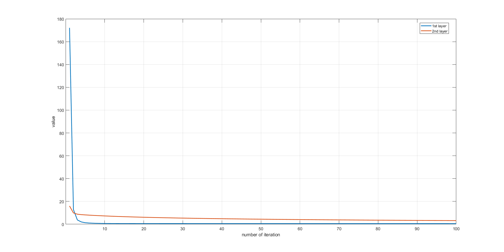
Figure 3: Convergence curve of CDLF on Extended YaleB dataset

$$\scriptsize\begin{split}&{\kern 10.0pt}f\left({{\left({{{\bf{C}}_{{l_{2}}}}}\right)_{m}},{\left({{{\bf{Z}}_{{l_{2}}}}}\right)_{m}},{\left({{{\bf{L}}_{{l_{2}}}}}\right)_{m}},{{\bf{B}}_{m}},{{\bf{W}}_{m}},{{\bf{A}}_{m}}}\right)\\ &\geq f\left({{\left({{{\bf{C}}_{{l_{2}}}}}\right)_{m+1}},{\left({{{\bf{Z}}_{{l_{2}}}}}\right)_{m+1}},{\left({{{\bf{L}}_{{l_{2}}}}}\right)_{m+1}},{{\bf{B}}_{m}},{{\bf{W}}_{m}},{{\bf{A}}_{m}}}\right)\\ &\geq f\left({{\left({{{\bf{C}}_{{l_{2}}}}}\right)_{m+1}},{\left({{{\bf{Z}}_{{l_{2}}}}}\right)_{m+1}},{\left({{{\bf{L}}_{{l_{2}}}}}\right)_{m+1}},{{\bf{B}}_{m+1}},{{\bf{W}}_{m+1}},{{\bf{A}}_{m+1}}}\right)\end{split}$$ (36)

3.5 Overall algorithm

The overall training procedures of our proposed framework is summarized in Algorithm 1. Here, $maxiter$ is the maximum number of iterations, ${\bf{1}}\in\mathbb{R}^{K_{1}\times K_{1}}$ is a square matrix with all elements 1 and $\odot$ indicates element dot product. ${\bf{Z}}$ represents the auxiliary variable, ${\bf{C}}$ is another form of ${\bf{S}}$ and ${\bf{L}}$ is augmented lagrange multiplier. In the algorithm 1, we first update the parameters of first layer to get the sparse codes ${{\bf{S}}_{{l_{1}}}}$ and dictionary ${{\bf{D}}_{{l_{1}}}}$. Then ${{\bf{S}}_{{l_{1}}}}$ is treated as one of the inputs of second layer to obtain the corresponding bases ${{\bf{D}}_{{l_{2}}}}$, ${\bf{W}}$.

Algorithm 1 Cascaded Dictionary Learning Framework

Input: ${{\bf{X}}}\in\mathbb{R}^{d\times N}$, ${\bf{H}}\in\mathbb{R}^{C\times N}$, ${\bf{Q}}\in\mathbb{R}^{K_{2}\times N}$
  Output: ${{\bf{D}}_{{l_{1}}}}\in\mathbb{R}^{d\times K_{{1}}}$, ${{\bf{D}}_{{l_{2}}}}\in\mathbb{R}^{d\times K_{{2}}}$, ${{\bf{W}}}\in\mathbb{R}^{C\times K_{{2}}}$,

1: Initialize $\left({{\bf{C}}_{{l_{1}}}^{c}}\right)_{0}$, $\left({{\bf{Z}}_{{l_{1}}}^{c}}\right)_{0}$, $\left({{\bf{L}}_{{l_{1}}}^{c}}\right)_{0}$

2: $m=0$

3: while $m\leq\max iter$ do

4:    $m\leftarrow m+1$

5:    Update ${{\bf{C}}_{{l_{1}}}^{c}}$, ${{\bf{Z}}_{{l_{1}}}^{c}}$, ${{\bf{L}}_{{l_{1}}}^{c}}$ with ADMM

6:    Update ${{\bf{D}}_{{l_{1}}}^{c}}$ with with BCD

7: end while

8: ${{\bf{D}}_{{l_{1}}}}\leftarrow\left[{{\bf{D}}_{{l_{1}}}^{1},{\bf{D}}_{{l_{1}}}^{2},\cdots,{\bf{D}}_{{l_{1}}}^{C}}\right]$; ${{\bf{S}}_{{l_{1}}}}\leftarrow\left[{{\bf{S}}_{{l_{1}}}^{1},{\bf{S}}_{{l_{1}}}^{2},\cdots,{\bf{S}}_{{l_{1}}}^{C}}\right]$

9: Initialize $\left({{\bf{C}}_{{l_{2}}}}\right)_{0}$, $\left({{\bf{Z}}_{{l_{2}}}}\right)_{0}$, $\left({{\bf{L}}_{{l_{2}}}}\right)_{0}$, $\left({{\bf{D}}_{{l_{2}}}}\right)_{0}$, $\left({{\bf{W}}_{{l_{2}}}}\right)_{0}$, $\left({{\bf{A}}_{{l_{2}}}}\right)_{0}$

10: $m=0$

11: while $m\leq\max iter$ do

12:    $m\leftarrow m+1$

13:    Update ${{\bf{C}}_{{l_{2}}}}$, ${{\bf{Z}}_{{l_{2}}}}$, ${{\bf{L}}_{{l_{2}}}}$ with ADMM

14:    Update ${{\bf{D}}_{{l_{2}}}},{\bf{W}},{\bf{A}}$ with BCD

15: end while

16: return  ${{\bf{D}}_{{l_{1}}}}$, ${{\bf{D}}_{{l_{2}}}}$, ${\bf{W}}$

In the testing stage, the constraint terms are based on $\ell_{1}$-norm sparse constraint. Here, we first exploit the learned dictionary ${\bf{D}}_{{l_{1}}}$ to fit the testing sample $\bf{y}$ and the output is the sparse codes ${{\bf{r}}_{{l_{1}}}}$. The formulation is shown in Equation 37.

$$\scriptsize\begin{split}{\bf{r}}_{l_{1}}=\arg{\min_{\bf{r}_{l_{1}}}}{\mkern 1.0mu}\left\{{\left\|{\bf{y}}-{\bf{D}_{l_{1}}}{\bf{r}_{l_{1}}}\right\|_{2}^{2}+2\alpha{{\left\|{\bf{r}_{l_{1}}}\right\|}_{1}}}\right\}\end{split}$$ (37)

Then the learned dictionary ${\bf{D}}_{{l_{2}}}$ are utilised to fit ${{\bf{r}}_{{l_{1}}}}$ and we can obtain the sparse codes ${{\bf{r}}_{{l_{2}}}}$. We show the objective function in Equation 38.

$$\scriptsize\begin{split}{\bf{r}}_{l_{2}}=\arg{\min_{\bf{r}_{l_{2}}}}{\mkern 1.0mu}\left\{{\left\|{\bf{r}_{l_{2}}}-{\bf{D}_{l_{2}}}{\bf{r}_{l_{2}}}\right\|_{2}^{2}+2\alpha{{\left\|{\bf{r}_{l_{2}}}\right\|}_{1}}}\right\}\end{split}$$ (38)

At last, we use the trained classfier ${\bf{W}}$ to predict the label of ${\bf{y}}$ which can be formulated as follows:

$$\scriptsize\begin{split}id\left({\bf{y}}\right)={\max}\left\{{{\bf{W}}{{\bf{r}}_{{l_{2}}}}}\right\}\end{split}$$ (39)

4 Experimental results

In this section, we evaluate the performance of our approach on several benchmark datasets, including two face datasets (Extented YaleB Georghiades et al. (2001) dataset, CMU PIE Sim et al. (2002) dataset), two handwritten digit datasets (MNIST LeCun et al. (1998) dataset and USPS Hull (1994) dataset) and two remote sensing datasets (RSSCB7 dataset Zou et al. (2015) and UC Mereced Land Use dataset Yang and Newsam (2010)), then compare it with other famous methods such as SVM Fan et al. (2008), SRC Wright et al. (2009), CRC Zhang et al. (2011), SLRC Deng et al. (2018), NRC Xu et al. (2019), Euler-SRC Song et al. (2018), ADDL Zhang et al. (2018), LC-PDL Zhang et al. (2019a), FDDL Yang et al. (2011), LC-KSVD Jiang et al. (2013), and CSDL-SRC Liu et al. (2016).

For all the experiments, we evaluate our methods by randomly selecting $5$ samples per class for training. Besides, to eliminate the randomness, we carry out every experiment $8$ times, and we report the mean of the classification rates.

For convenience, we fix the dictionary sizes($K_{1}$ and $K_{2}$) to twice the number of training samples. Moreover, there are four other parameters($\zeta$, $\lambda$, $\omega$, $\varepsilon$) that need to be adjusted to achieve the highest classification rates. The details are shown in the following subsections. In the next subsection, we illustrate the experimental results on the six datasets. Moreover, some discussions are finally listed.

4.1 Extended YaleB dataset

The Extended YaleB dataset is consists of $2{,}432$ face images from 38 individuals, each having around 64 nearly frontal images under varying illumination conditions. Here, we resize each image to $32\times 32$ pixels and then pull them into column vectors. After that, we normalize the images to form the raw $\ell_{2}$ normalized features. Figure 4 $a$ shows some images of the dataset.

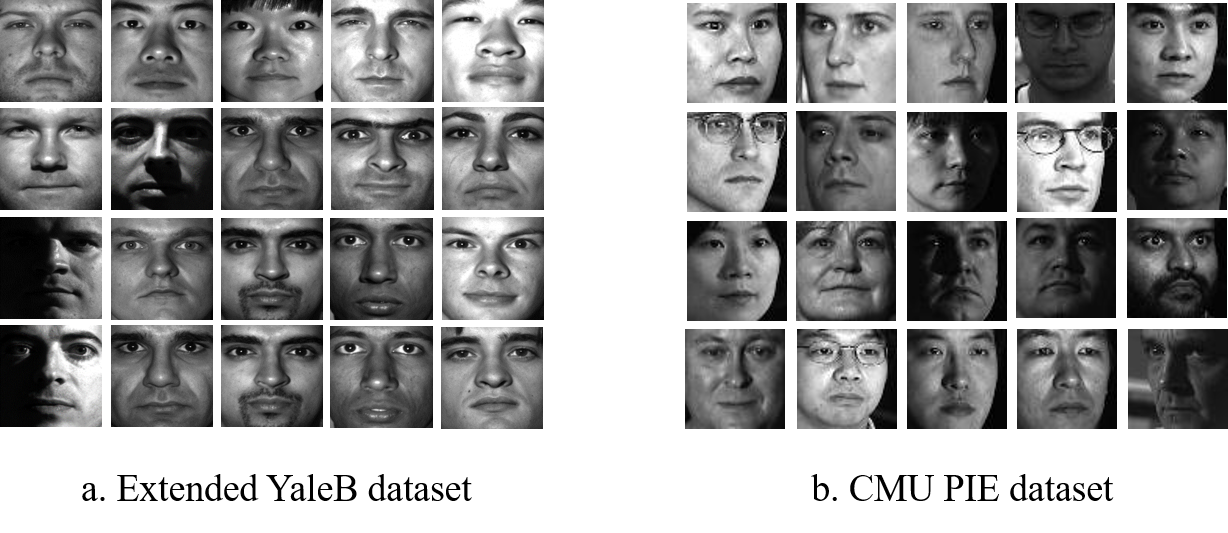
Figure 4: Examples of the face datasets

In addition, we set $\lambda={2^{-3}}$, $\omega={2^{-11}}$ and $\varepsilon={2^{-8}}$ for LEDL algorithm and set $\zeta={2^{-10}}$, $\lambda={2^{-6}}$, $\omega={2^{-10}}$ and $\varepsilon={2^{-8}}$ in our experiment to achieve highest accuracy for both algorithms, respectively. The experimental results are summarized in Table 1. From Table 1, we can see that our proposed LEDL and CDLF algorithms achieve superior performance to other methods. Compared with some conventional algorithms which the DL method is not involved in such as SVM, SRC, CRC, SLRC, NRC, and Euler-SRC, the classification performance is improved by $2.1\%$ and $2.9\%$ with our proposed LEDL algorithm and CDLF algorithm, respectively. Compared with five classical DL based algorithms, including ADDL, LC-PDL, FDDL, LC-KSVD, and CSDL-SRC, our proposed LEDL algorithm and CDLF algorithm exceeds $1.1\%$ and $1.9\%$, respectively. Additionally, the classification performance of CDLF algorithm exceeds that of LEDL algorithm by $0.8\%$.

Table 1: Classification rates ($\%$) on face datasets

Methods	Extended YaleB	CMU PIE
SVM Fan et al. (2008)	$73.6$	$71.8$
SRC Wright et al. (2009)	$79.1$	$73.7$
CRC Zhang et al. (2011)	$79.2$	$73.3$
SLRC Deng et al. (2018)	$76.7$	$70.1$
NRC Xu et al. (2019)	$76.1$	$71.0$
Euler-SRC Song et al. (2018)	$78.5$	$74.4$
ADDL Zhang et al. (2018)	$77.4$	$71.1$
LC-PDL Zhang et al. (2019a)	$77.5$	$70.2$
FDDL Yang et al. (2011)	$76.8$	$70.7$
LC-KSVD Jiang et al. (2013)	$73.5$	$67.1$
CSDL-SRC Liu et al. (2016)	$80.2$	$77.4$
Our LEDL	$81.3$	$77.7$
Our CDLF	$\bf 82.1$	$\bf 78.7$

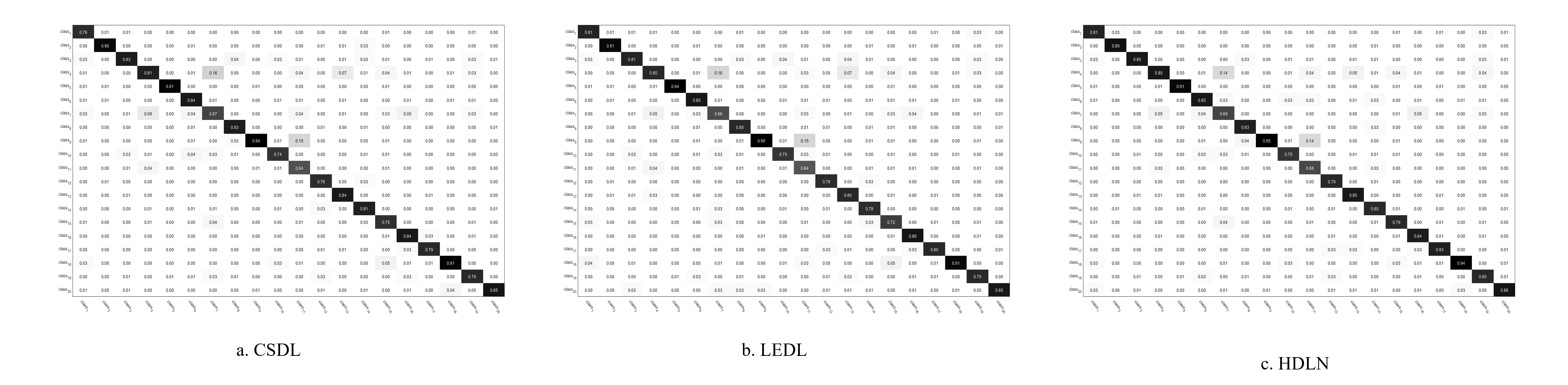
Figure 8: Confusion matrices on Extended YaleB dataset

To further illustrate the superiority of our proposed CDLF, we choose the first 20 classes’ samples of the Extended YaleB dataset as a sub-dataset to build a confusion matrix. Figure 8 show the confusion matrices of different methods. As can be seen, our method achieves a higher classification rate in most of the chosen $20$ classes. More specifically, for some classes such as class3, class 4, class 11, class 15, class 17, we get poor classification rates by utilizing CSDL-SRC and LEDL separately. However, there are notable gains while using CDLF. And for some classes (class 1, class 6, class 8, class 9, class 10), which the accuracies have large differences between CSDL-SRC and LEDL, the classification rate of CDLF is similar to the result of the optimal one of CSDL-SRC and LEDL.

4.2 CMU PIE dataset

The CMU PIE dataset contains $41{,}368$ images of $68$ individuals with $43$ different illumination conditions. Each human is under $13$ different poses and with $4$ different expressions. Like the Extended YaleB dataset, each face image is cropped to $32\times 32$ pixels, pulled into column vectors, and normalized to $1$. Several samples from this dataset are listed in Figure 4 $b$.

The results are shown in Table 1, as can be seen that our methods outperforms all the competing approaches by setting $\lambda={2^{-3}}$, $\omega={2^{-11}}$, $\varepsilon={2^{-8}}$ for LEDL algorithm and $\zeta={2^{-12}}$, $\lambda={2^{-5}}$, $\omega={2^{-11}}$, $\varepsilon={2^{-3}}$ for CDLF algorithm. Specifically, our proposed method achieves an improvement of at least $3.3\%$ and $4.3\%$ over some traditional methods such as SVM, SRC, CRC, SLRC, NRC, and Euler-SRC for LEDL algorithm and CDLF algorithm, respectively. Compared with DL based methods, our proposed LEDL algorithm and CDLF algorithm exceed the other algorithms at least $0.3\%$ and $1.3\%$, respectively. Futhermore, we reduce the dimensionality using t-distributed Stochastic Neighbor Embedding(t-SNE) Maaten and Hinton (2008) to show the distribution of the feature extracted from PIE dataset. The results are shown in Figure 5, it is clear to see the distinction among the categories after our proposed method.

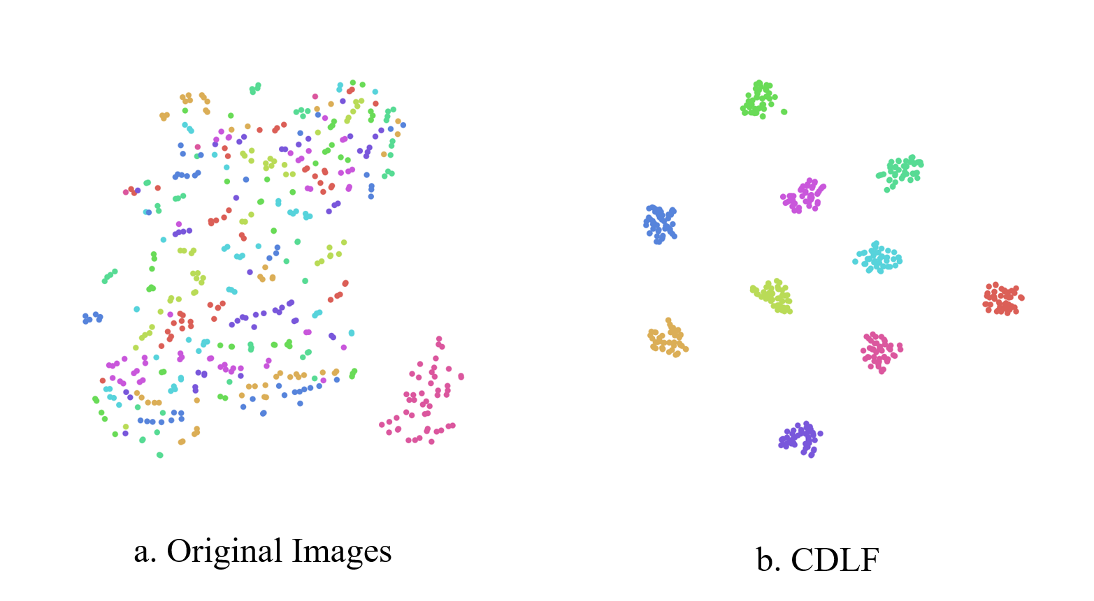
Figure 5: t-SNE visualization

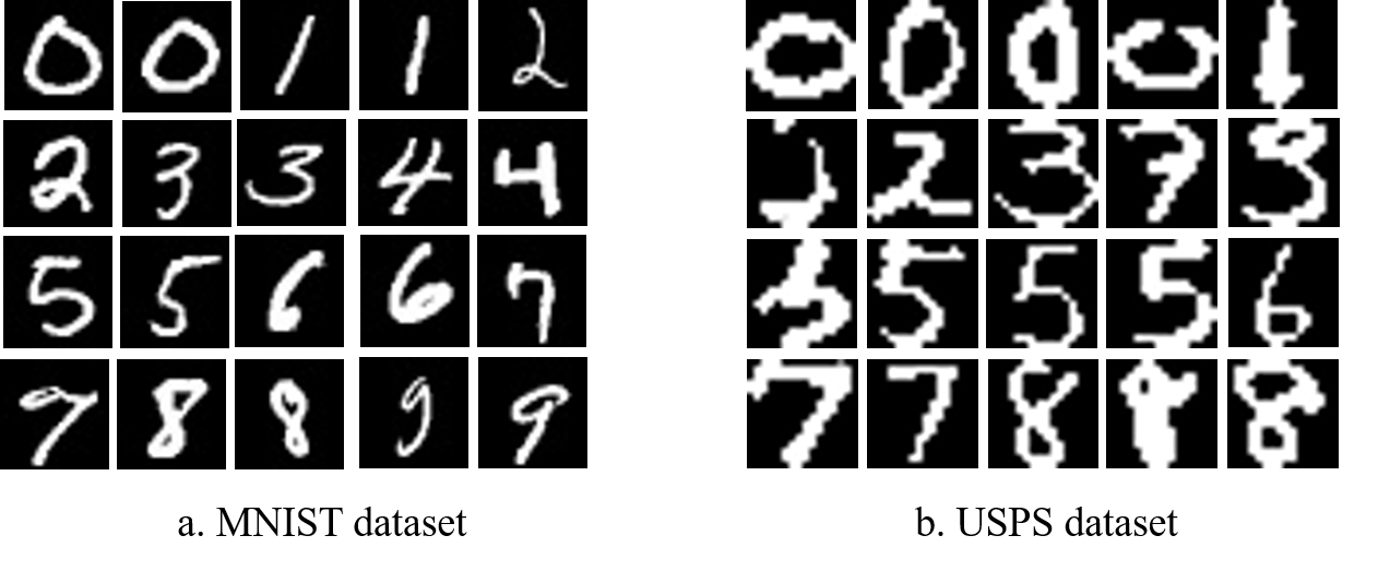
Figure 6: Examples of the handwritten digit datasets

Table 2: Classification rates ($\%$) on handwritten digit datasets

Methods	MNIST	USPS
SVM Fan et al. (2008)	$65.4$	$78.8$
SRC Wright et al. (2009)	$69.8$	$78.4$
CRC Zhang et al. (2011)	$68.3$	$77.9$
SLRC Deng et al. (2018)	$66.5$	$76.4$
NRC Xu et al. (2019)	$68.5$	$76.2$
Euler-SRC Song et al. (2018)	$65.9$	$76.1$
ADDL Zhang et al. (2018)	$64.9$	$65.6$
LC-PDL Zhang et al. (2019a)	$60.5$	$63.2$
FDDL Yang et al. (2011)	$62.4$	$76.2$
LC-KSVD Jiang et al. (2013)	$62.1$	$71.1$
CSDL-SRC Liu et al. (2016)	$69.8$	$78.8$
Our LEDL	$69.8$	$81.1$
Our CDLF	$\bf 70.3$	$\bf 81.9$

4.3 MNIST dataset

The MNIST dataset includes $70{,}000$ images for digit numbers from $0$ to $9$. Here, we pull the original images in which the size is $28\times 28$ into column vectors. There are some samples from the dataset are given in Figure 6 $a$.

In Tabel 2, we can see that the classification rates of some conventional methods such as SVM, SRC, CRC, SLRC, NRC, and Euler-SRC can achieve the similar ones of DL based methods (e.g. the classification rates between SRC, CSDL-SRC, and LEDL are similar). However, our proposed CDLF can achieve the highest accuracy by an improvement of at least $0.5\%$ compared with all the methods in Tabel 2. The optimal parameter for LEDL algorithm are $\lambda={2^{-8}}$, $\omega={2^{-14}}$, $\varepsilon={2^{-4}}$ and the optimal parameters for CDLF algorithm are $\zeta={2^{-8}}$, $\lambda={2^{-6}}$, $\omega={2^{-6}}$, $\varepsilon={2^{-2}}$.

4.4 USPS dataset

The USPS dataset consists of $9{,}298$ handwritten digit images from $0$ to $9$, which come from the U.S. Postal System. For the USPS dataset, the images are resized into $16\times 16$ and pulled into column vectors. Several samples from this dataset are listed in Figure 6 $b$.

The results are showed in Tabel 2. For LEDL algorithm, we adjust $\lambda={2^{-4}}$, $\omega={2^{-8}}$, $\varepsilon={2^{-5}}$. For CDLF algorithm, we adjust $\zeta={2^{-11}}$, $\lambda={2^{-10}}$, $\omega={2^{-14}}$, $\varepsilon={2^{-8}}$ to achieve the highest accuracy. Compared with the methods (SVM, SRC, CRC, SLRC, NRC, and Euler-SRC) which the DL is not added into the classifiers, CDLF algorithm achieves an improvement of at least $3.1\%$ and LEDL algorithm achieves an improvement of at least $2.3\%$. Compared with the DL based method, LEDL algorithm achieves an improvement of $3.1\%$.

4.5 RSSCN7 dataset

The RSSCN7 dataset consists of seven different RS scene categories of $2,800$ aerial-scene images in total, which are grassland, forest, farmland, industry, parking lot, residential, river, and lake region. Each class included $400$ images, and all images are of the same size of $400\times 400$ pixels. Here, we use the Resnet model He et al. (2016) to extract the features. Specifically, the layer $pool5$ is utilized to extract $2,048$-dimensional vectors for them. Figure 7 $a$ shows several samples belongs to this dataset.

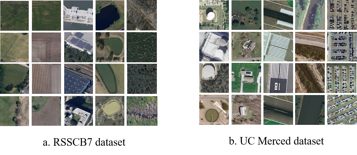
Figure 7: Examples of the remote sensing datasets

Table 3: Classification rates ($\%$) on remote sensing datasets

Methods	RSSCB7	UC Mereced
SVM Fan et al. (2008)	$67.5$	$80.5$
SRC Wright et al. (2009)	$67.1$	$80.4$
CRC Zhang et al. (2011)	$67.7$	$80.7$
SLRC Deng et al. (2018)	$66.4$	$80.9$
NRC Xu et al. (2019)	$65.5$	$79.6$
Euler-SRC Song et al. (2018)	$67.0$	$80.6$
ADDL Zhang et al. (2018)	$\bf 72.3$	$\bf 83.2$
LC-PDL Zhang et al. (2019a)	$69.7$	$81.2$
FDDL Yang et al. (2011)	$60.0$	$81.0$
LC-KSVD Jiang et al. (2013)	$68.0$	$79.4$
CSDL-SRC Liu et al. (2016)	$66.6$	$80.5$
Our LEDL	$67.9$	$80.7$
Our CDLF	$69.6$	$81.0$

Table 4: Classification rates ($\%$) on remote sensing datasets

Methods	Extended YaleB	CMUPIE	MNIST	USPS	RSSCB7	UC Mereced
SVM Fan et al. (2008)	$73.6$	$71.8$	$65.4$	$78.8$	$67.5$	$80.5$
SRC Wright et al. (2009)	$79.1$	$73.7$	$69.8$	$78.4$	$67.1$	$80.4$
CRC Zhang et al. (2011)	$79.2$	$73.3$	$68.3$	$77.9$	$67.7$	$80.7$
SLRC Deng et al. (2018)	$76.7$	$70.1$	$65.5$	$76.4$	$66.4$	$80.9$
NRC Xu et al. (2019)	$76.1$	$71.0$	$68.5$	$76.2$	$65.5$	$79.6$
Euler-SRC Song et al. (2018)	$78.5$	$74.4$	$65.9$	$76.1$	$67.0$	$80.6$
ADDL Zhang et al. (2018)	$77.4$	$71.1$	$64.9$	$65.6$	$\bf 72.3$	$\bf 83.2$
LC-PDL Zhang et al. (2019a)	$77.5$	$70.2$	$60.5$	$63.2$	$69.7$	$81.2$
FDDL Yang et al. (2011)	$76.8$	$70.7$	$62.4$	$76.2$	$60.0$	$81.0$
LC-KSVD Jiang et al. (2013)	$73.5$	$67.1$	$62.1$	$71.1$	$68.0$	$79.4$
CSDL-SRC Liu et al. (2016)	$80.2$	$77.4$	$69.8$	$78.8$	$66.6$	$80.5$
LEDL Shao et al. (2020)	$81.3$	$77.7$	$69.8$	$81.1$	$67.9$	$80.7$
Our CDLF	$\bf 82.1$	$\bf 78.7$	$\bf 70.3$	$\bf 81.9$	$69.6$	$81.0$

Table 4 shows the experimental results. It is clearly to see that only three methods (ADDL, LC-PDL, and CSDL) can gain good performance. We will illustrate the analysis why the performance of our methods is lower than that of ADDL in 4.7. The optimal parameters are $\lambda={2^{-8}}$, $\omega={2^{-14}}$, $\varepsilon={2^{-14}}$ for LEDL algorithm. And the optimal parameters are $\zeta={2^{-13}}$, $\lambda={2^{-3}}$, $\omega={2^{-11}}$, $\varepsilon={2^{-11}}$ for CDLF algorithm.

4.6 UC Mereced Land Use dataset

The UC Merced Land Use Dataset contains a total of $2,100$ land-use images. The dataset is collected from the United States Geological Survey National Map of 20 U.S. regions. The size of each original image is $256\times 256$ pixels. Here, we also use the Resnet model to obtain 2048-dimensional vectors. Some samples are listed in Figure 7 $b$.

Table 4 shows the classification rates of different methods. Without considering ADDL, it is hard to say that the DL method contributes a lot for image classification in this dataset. Whether LC-KSVD, CSDL-SRC, and LEDL can not get better performance than traditional methods such as SVM, SRC, CRC, SLRC, NRC, and Euler-SRC. Only LC-PDL and our proposed CDLF algorithm can achieve a slight improvement. The comparison with ADDL is summarized in 4.7.

4.7 Analysis and discussion

In this section, we mainly focus on illustrating ablation learning and analysis of the experimental results.

4.7.1 Ablation learning

To further evaluate the necessity of each term in Equation 3, we show the ablation experiments on two face datasets in Figure LABEL:fig:_Ablation_experiments. The results demonstrate that all terms contribute a lot to our approach.

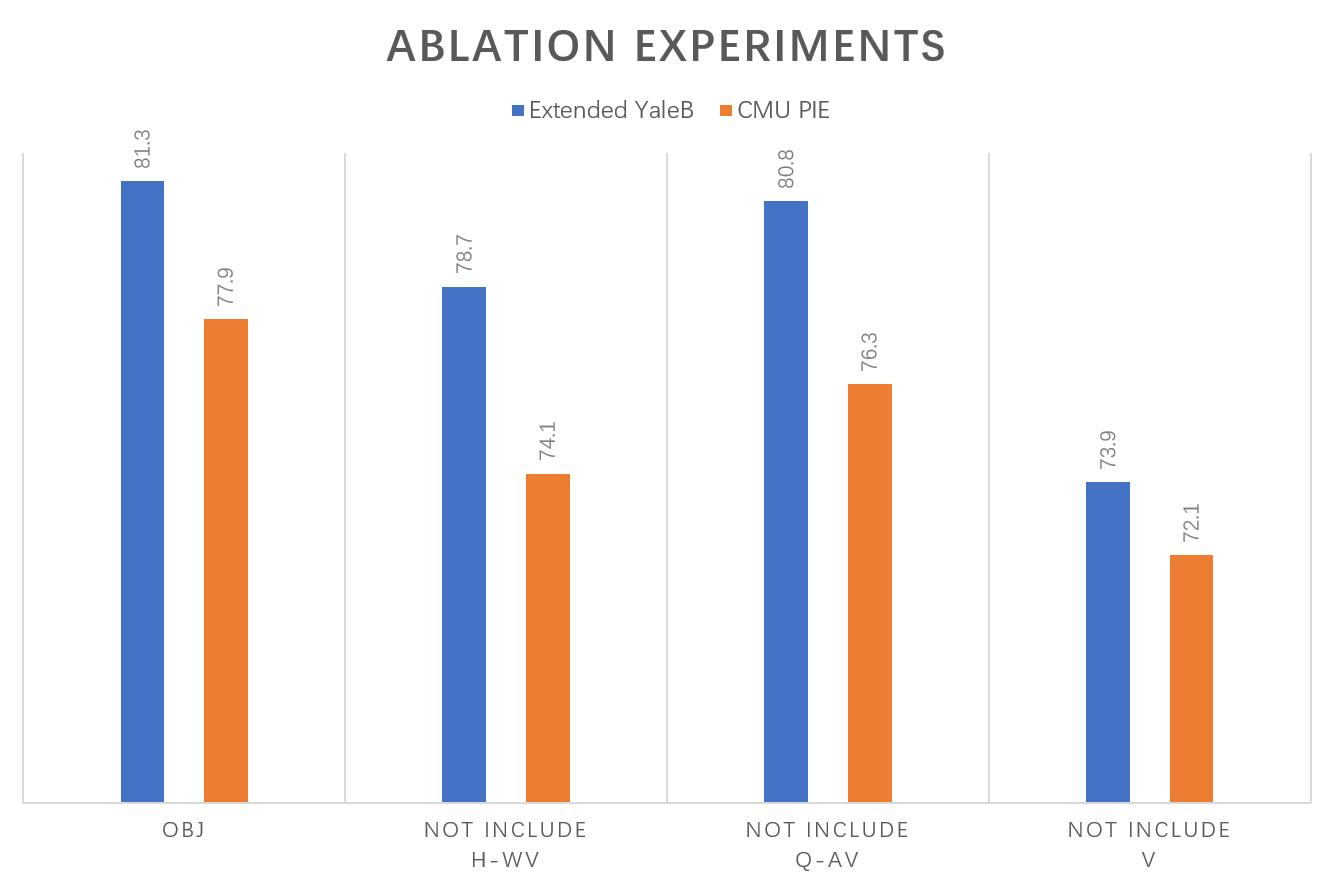
Figure 9: Ablation experiments in LEDL

4.7.2 Analysis of experimental results

We can see that our proposed methods have significant improvement compared with other classical methods except for ADDL on remote sensing datasets. The reason is that ADDL encourages the subdictionaries associated with different classes to be independent while our approaches focus more on global information. Thus, ADDL is more applicable to the datasets, which have significant differences among categories. At the same time, remote sensing datasets usually consist of images that come from different regions. Each class is very different. That is why ADDL can gain better performance than our proposed CDLF on the two specific datasets.

On the other hand, we have demonstrated on various datasets that our proposed CDLF is more general than other methods. However, it is not easy to obtain cleaned datasets in the real world. Besides, the computational complexity of the algorithm is an essential factor to consider in practical applications. To further validate the performance of our proposed methods, we give the following analysis:

1) We add Gaussian noise with different variances ($0.2$, $0.4$, $0.6$) to the Extended YaleB dataset to simulate actual data. Figure 10 shows several examples. Table 5 shows the experimental results. It is clear to see that our proposed methods are less sensitive to noise than other methods.

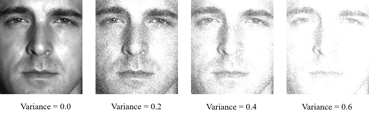
Figure 10: Examples of the noisy Extended YaleB dataset

Table 5: Classification rates ($\%$) on noisy Extended YaleB dataset

Methods$\backslash$Variance	0.0	0.2	0.4	0.6
SVM Fan et al. (2008)	$73.6$	$70.5$	$69.8$	$67.9$
SRC Wright et al. (2009)	$79.1$	$70.2$	$60.1$	$36.7$
CRC Zhang et al. (2011)	$79.2$	$76.2$	$75.6$	$74.1$
SLRC Deng et al. (2018)	$76.7$	$66.4$	$51.1$	$19.5$
NRC Xu et al. (2019)	$76.1$	$74.1$	$70.9$	$63.3$
Euler-SRC Song et al. (2018)	$78.5$	$76.8$	$76.5$	$75.5$
ADDL Zhang et al. (2018)	$77.4$	$65.5$	$51.7$	$38.6$
LC-PDL Zhang et al. (2019a)	$77.5$	$65.2$	$50.9$	$38.7$
FDDL Yang et al. (2011)	$76.8$	$64.2$	$46.8$	$30.0$
LC-KSVD Jiang et al. (2013)	$73.5$	$74.1$	$69.4$	$66.3$
CSDL-SRC Liu et al. (2016)	$80.2$	$\bf{85.3}$	$78.1$	$73.2$
LEDL	$81.3$	$79.6$	$79.5$	$76.1$
CDLF	$\bf{82.1}$	$80.9$	$\bf{81.6}$	$\bf{76.8}$

2) We list the computational complexity of some methods in Table 6. $N$ is the number of training samples, $D$ represents the dimensions of the sample features, $K$ is the number of atoms in the dictionary, $T$ is the sparsity constraint factor, $K^{c}$ and $N^{c}$ represent the $c_{th}$ class of $N$ and $K$, respectively. In our experiments, $K$ is twice the number of $N$ and $K>N>D>T$. From the table, we can say that the complexity of our methods is slightly higher than some traditional methods in some cases, which depends on the size of $K$.

Table 6: Computational Complexity

Methods	Complexity
${\mathbf{SRC}}$	$O(N^{2}D)$
${\mathbf{CRC}}$	$O(N^{2}D)$
${\mathbf{SLRC}}$	$O(N^{2}D)$
${\mathbf{CSDL-SRC}}$	$O(K^{c}N^{c}D)$
${\mathbf{LC-KSVD}}$	$O(KN^{2}DT)$
${\mathbf{LEDL}}$	$O(KND)$
${\mathbf{CDLF}}$	$O(KND)$

The analysis above illustrates that our methods are more suitable for practical situations compared to other approaches to some extent.

5 Conclusion

In this paper, we first propose a novel class shared dictionary learning method named label embedded dictionary learning (LEDL). This method introduces the $\ell_{1}$-norm regularization term to replace the $\ell_{0}$-norm regularization of LC-KSVD. Then we propose a novel network named hybrid dictionary learning network (CDLF) to combine a class specific dictionary learning method with a class shared dictionary learning method to describe the feature to boost the classification performance. Besides, we adopt the ADMM algorithm to solve the $\ell_{1}$-norm optimization problem and the BCD algorithm to update the corresponding dictionaries. Finally, extensive experiments on six well-known benchmark datasets have proved the superiority of our proposed LEDL and CDLF methods.

6 Acknowledgment

This research was funded by the National Natural Science Foundation of China (Grant No. 61402535, No. 61271407), the Natural Science Foundation of Shandong Province, China(Grant No. No. ZR2019MF073, ZR2018MF017, ZR2017MF069), Qingdao Science and Technology Project (No. 17-1-1-8-jch), the Fundamental Research Funds for the Central Universities, China University of Petroleum (East China) (Grant No. 20CX05001A, 17CX02027A), the Open Research Fund from Shandong Provincial Key Laboratory of Computer Network (No. SDKLCN-2018-01), the Major Scientific and Technological Projects of CNPC (No. ZD2019-183-008), and the Creative Research Team of Young Scholars at Universities in Shandong Province (No.2019KJN019).

References

- Aharon et al. (2006) Aharon, M., Elad, M., Bruckstein, A., et al., 2006. K-svd: An algorithm for designing overcomplete dictionaries for sparse representation. IEEE Transactions on Signal Processing 54, 4311–4322.
- Akhtar et al. (2016) Akhtar, N., Shafait, F., Mian, A., 2016. Discriminative bayesian dictionary learning for classification. IEEE Transactions on Pattern Analysis and Machine Intelligence 38, 2374–2388.
- Boyd et al. (2011) Boyd, S., Parikh, N., Chu, E., Peleato, B., Eckstein, J., 2011. Distributed optimization and statistical learning via the alternating direction method of multipliers. Foundations and Trends® in Machine learning 3, 1–122.
- Chan et al. (2015) Chan, T.H., Jia, K., Gao, S., Lu, J., Zeng, Z., Ma, Y., 2015. Pcanet: A simple deep learning baseline for image classification? IEEE Transactions on Image Processing 24, 5017–5032.
- Deng et al. (2018) Deng, W., Hu, J., Guo, J., 2018. Face recognition via collaborative representation: Its discriminant nature and superposed representation. IEEE Transactions on Pattern Analysis and Machine Intelligence 40, 2513–2521.
- Fan et al. (2008) Fan, R.E., Chang, K.W., Hsieh, C.J., Wang, X.R., Lin, C.J., 2008. Liblinear: A library for large linear classification. Journal of Machine Learning Research 9, 1871–1874.
- Gao et al. (2018) Gao, D., Hu, Z., Ye, R., 2018. Self-dictionary regression for hyperspectral image super-resolution. Remote Sensing 10, 1574–1596.
- Georghiades et al. (2001) Georghiades, A.S., Belhumeur, P.N., Kriegman, D.J., 2001. From few to many: Illumination cone models for face recognition under variable lighting and pose. IEEE Transactions on Pattern Analysis and Machine Intelligence 23, 643–660.
- Gu et al. (2014) Gu, S., Zhang, L., Zuo, W., Feng, X., 2014. Projective dictionary pair learning for pattern classification, in: Advances in neural information processing systems, pp. 793–801.
- He et al. (2016) He, K., Zhang, X., Ren, S., Sun, J., 2016. Deep residual learning for image recognition, in: IEEE conference on Computer Vision and Pattern Recognition (CVPR), IEEE. pp. 770–778.
- Hull (1994) Hull, J.J., 1994. A database for handwritten text recognition research. IEEE Transactions on Pattern Analysis and Machine Intelligence 16, 550–554.
- Jiang et al. (2019) Jiang, K., Wang, Z., Yi, P., Wang, G., Lu, T., Jiang, J., 2019. Edge-enhanced gan for remote sensing image superresolution. IEEE Transactions on Geoscience and Remote Sensing (TGRS) 57, 5799–5812.
- Jiang et al. (2017) Jiang, W., Zhang, Z., Qin, J., Zhao, M., Li, F., Yan, S., 2017. Robust projective dictionary learning by joint label embedding and classification, in: 2017 IEEE International Conference on Data Mining Workshops (ICDMW), IEEE. pp. 510–517.
- Jiang et al. (2013) Jiang, Z., Lin, Z., Davis, L.S., 2013. Label consistent k-svd: Learning a discriminative dictionary for recognition. IEEE Transactions on Pattern Analysis and Machine Intelligence 35, 2651–2664.
- LeCun et al. (1998) LeCun, Y., Bottou, L., Bengio, Y., Haffner, P., et al., 1998. Gradient-based learning applied to document recognition. Proceedings of the IEEE 86, 2278–2324.
- Li et al. (2018) Li, H., He, X., Tao, D., Tang, Y., Wang, R., 2018. Joint medical image fusion, denoising and enhancement via discriminative low-rank sparse dictionaries learning. Pattern Recognition 79, 130–146.
- Li et al. (2012) Li, S., Fang, L., Yin, H., 2012. An efficient dictionary learning algorithm and its application to 3-d medical image denoising. IEEE Transactions on Biomedical Engineering 59, 417–427.
- Li et al. (2019) Li, Z., Zhang, Z., Qin, J., Zhang, Z., Shao, L., 2019. Discriminative fisher embedding dictionary learning algorithm for object recognition. IEEE Transactions on Neural Networks and Learning Systems .
- Lin et al. (2018) Lin, G., Yang, M., Yang, J., Shen, L., Xie, W., 2018. Robust, discriminative and comprehensive dictionary learning for face recognition. Pattern Recognition 81, 341–356.
- Liu et al. (2019) Liu, B., Jing, L., Li, J., Yu, J., Gittens, A., Mahoney, M.W., 2019. Group collaborative representation for image set classification. International Journal of Computer Vision 127, 181–206.
- Liu et al. (2017) Liu, B.D., Gui, L., Wang, Y., Wang, Y.X., Shen, B., Li, X., Wang, Y.J., 2017. Class specific centralized dictionary learning for face recognition. Multimedia Tools and Applications 76, 4159–4177.
- Liu et al. (2016) Liu, B.D., Shen, B., Gui, L., Wang, Y.X., Li, X., Yan, F., Wang, Y.J., 2016. Face recognition using class specific dictionary learning for sparse representation and collaborative representation. Neurocomputing 204, 198–210.
- Liu et al. (2014) Liu, B.D., Wang, Y.X., Shen, B., Zhang, Y.J., Wang, Y.J., 2014. Blockwise coordinate descent schemes for sparse representation, in: IEEE International conference on Acoustics, Speech and Signal Processing (ICASSP), IEEE. pp. 5267–5271.
- Maaten and Hinton (2008) Maaten, L.v.d., Hinton, G., 2008. Visualizing data using t-sne. Journal of machine learning research 9, 2579–2605.
- Mallat and Zhang (1993) Mallat, S.G., Zhang, Z., 1993. Matching pursuit with time-frequency dictionaries. IEEE Transactions on Signal Processing 41, 3397–3415.
- Olshausen and Field (1996) Olshausen, B.A., Field, D.J., 1996. Emergence of simple-cell receptive field properties by learning a sparse code for natural images. Nature 381, 607–609.
- Olshausen and Field (1997) Olshausen, B.A., Field, D.J., 1997. Sparse coding with an overcomplete basis set: a strategy employed by v1? Vision Research 37, 3311–3325.
- Ren et al. (2020) Ren, J., Zhang, Z., Li, S., Wang, Y., Liu, G., Yan, S., Wang, M., 2020. Learning hybrid representation by robust dictionary learning in factorized compressed space. IEEE Transactions on Image Processing .
- Sim et al. (2002) Sim, T., Baker, S., Bsat, M., 2002. The cmu pose, illumination, and expression (pie) database, in: IEEE International conference on Automatic Face and Gesture Recognition (FG), IEEE. pp. 53–58.
- Song et al. (2018) Song, Y., Liu, Y., Gao, Q., Gao, X., Nie, F., Cui, R., 2018. Euler label consistent k-svd for image classification and action recognition. Neurocomputing 310, 277–286.
- Sun et al. (2020) Sun, Y., Zhang, Z., Jiang, W., Zhang, Z., Zhang, L., Yan, S., Wang, M., 2020. Discriminative local sparse representation by robust adaptive dictionary pair learning. IEEE Transactions on Neural Networks and Learning Systems .
- Tropp and Gilbert (2007) Tropp, J.A., Gilbert, A.C., 2007. Signal recovery from random measurements via orthogonal matching pursuit. IEEE Transactions on Information Theory 53, 4655–4666.
- Wright et al. (2009) Wright, J., Yang, A.Y., Ganesh, A., Sastry, S.S., Ma, Y., 2009. Robust face recognition via sparse representation. IEEE Transactions on Pattern Analysis and Machine Intelligence 31, 210–227.
- Xu et al. (2019) Xu, J., An, W., Zhang, L., Zhang, D., 2019. Sparse, collaborative, or nonnegative representation: Which helps pattern classification? Pattern Recognition 88, 679–688.
- Yang et al. (2009) Yang, J., Yu, K., Gong, Y., Huang, T., 2009. Linear spatial pyramid matching using sparse coding for image classification, in: IEEE conference on Computer Vision and Pattern Recognition (CVPR), IEEE. pp. 1794–1801.
- Yang et al. (2011) Yang, M., Zhang, L., Feng, X., Zhang, D., 2011. Fisher discrimination dictionary learning for sparse representation, in: International Conference on Computer Vision, IEEE. pp. 543–550.
- Yang and Newsam (2010) Yang, Y., Newsam, S., 2010. Bag-of-visual-words and spatial extensions for land-use classification, in: ACM International conference on Advances in Geographic Information Systems (GIS), ACM. pp. 270–279.
- Zhang et al. (2011) Zhang, L., Yang, M., Feng, X., 2011. Sparse representation or collaborative representation: Which helps face recognition?, in: IEEE International conference on Computer Vision (ICCV), IEEE. pp. 471–478.
- Zhang and Li (2010) Zhang, Q., Li, B., 2010. Discriminative k-svd for dictionary learning in face recognition, in: IEEE conference on Computer Vision and Pattern Recognition (CVPR), IEEE. pp. 2691–2698.
- Zhang et al. (2018) Zhang, Z., Jiang, W., Qin, J., Zhang, L., Li, F., Zhang, M., Yan, S., 2018. Jointly learning structured analysis discriminative dictionary and analysis multiclass classifier. IEEE Transactions on Neural Networks and Learning Systems 29, 3798–3814.
- Zhang et al. (2019a) Zhang, Z., Jiang, W., Zhang, Z., Li, S., Liu, G., Qin, J., 2019a. Scalable block-diagonal locality-constrained projective dictionary learning, in: International Joint Conference on Artificial Intelligence (IJCAI), pp. 4376–4382.
- Zhang et al. (2016) Zhang, Z., Li, F., Chow, T.W., Zhang, L., Yan, S., 2016. Sparse codes auto-extractor for classification: A joint embedding and dictionary learning framework for representation. IEEE Transactions on Signal Processing 64, 3790–3805.
- Zhang et al. (2019b) Zhang, Z., Ren, J., Jiang, W., Zhang, Z., Hong, R., Yan, S., Wang, M., 2019b. Joint subspace recovery and enhanced locality driven robust flexible discriminative dictionary learning. IEEE Transactions on Circuits and Systems for Video Technology .
- Zhang et al. (2020) Zhang, Z., Sun, Y., Wang, Y., Zha, Z., Yan, S., Wang, M., 2020. Convolutional dictionary pair learning network for image representation learning, in: European Conference on Artificial Intelligence (ECAI).
- Zhang et al. (2019c) Zhang, Z., Sun, Y., Zhang, Z., Wang, Y., Liu, G., Wang, M., 2019c. Learning structured twin-incoherent twin-projective latent dictionary pairs for classification, in: IEEE International Conference on Data Mining (ICDM).
- Zou et al. (2015) Zou, Q., Ni, L., Zhang, T., Wang, Q., 2015. Deep learning based feature selection for remote sensing scene classification. IEEE Geoscience and Remote Sensing Letters 12, 2321–2325.