On the magnitude and intrinsic volumes of a convex body in Euclidean space
Abstract.
Magnitude is an isometric invariant of metric spaces inspired by category theory. Recent work has shown that the asymptotic behavior under rescaling of the magnitude of subsets of Euclidean space is closely related to intrinsic volumes. Here we prove an upper bound for the magnitude of a convex body in Euclidean space in terms of its intrinsic volumes. The result is deduced from an analogous known result for magnitude in , via approximate embeddings of Euclidean space into high-dimensional spaces. As a consequence, we deduce a sufficient condition for infinite-dimensional subsets of a Hilbert space to have finite magnitude. The upper bound is also shown to be sharp to first order for an odd-dimensional Euclidean ball shrinking to a point; this complements recent work investigating the asymptotics of magnitude for large dilatations of sets in Euclidean space.
1. Introduction and main results
Magnitude is an isometric invariant of metric spaces defined by Leinster [16] based on category-theoretic considerations. It is an abstract notion of the size of a metric space, which in some ways serves as an “effective number of points” in the space. Magnitude turns out to encode many classical invariants from integral geometry and geometric measure theory, including volume, capacity, dimension, and surface area. See [19] for a survey of connections between magnitude and geometry. In other directions, magnitude has connections to graph invariants [17], theoretical ecology [27, 18], and homology theory [13, 20, 25, 12, 3].
The purpose of this note is to show that the magnitude of a convex body (i.e., a nonempty compact convex set) in the -dimensional Euclidean space is bounded above by a particular linear combination of the intrinsic volumes of (Theorem 1). The only such sets whose magnitudes are known explicitly are Euclidean balls for odd , and even in those cases the statement for arbitrary odd is quite complicated [1, 31] (see Theorem 11 below).
The upper bound in Theorem 1 can be used to show that certain infinite-dimensional compact sets in a Hilbert space have finite magnitude, specifically, so-called Gaussian bounded sets (Corollary 2). The bound is also sharp to first order for odd-dimensional Euclidean balls with small radius, as shown in Theorem 4. These results can be used to clarify the asymptotic behavior of the magnitude of a convex body in as it shrinks to a point (Corollaries 3 and 6).
Magnitude can be defined in several equivalent ways (see [19]). For the purposes of this paper the following will suffice. A metric space is called positive definite if, for each and each collection of distinct , the matrix is positive definite. Every subset of for is positive definite; this of course includes subsets of , the space equipped with the metric for . (See [23, Theorem 3.6] for a broad list of positive definite metric spaces.) If is a compact positive definite metric space, then the magnitude of is
| (1) |
It is an open question whether this supremum is finite for every compact positive definite metric space.
For , the intrinsic volumes of a convex body can be defined by the Kubota formula
| (2) |
where is the Grassmann manifold of -dimensional subspaces of , denotes the rotation-invariant probability measure on , denotes the orthogonal projection onto , and
is the volume of the unit ball in ; see e.g. [26, p. 222].
The normalization of the intrinsic volumes is chosen such that if is an isometric embedding and is a convex body, then for all . It follows that is well-defined for any finite-dimensional convex body in a Hilbert space . For a general convex body , we define
The first main result of this paper is the following.
Theorem 1.
If is a convex body, then
| (3) |
with equality if .
Theorem 1 can be compared to the erstwhile conjecture (see [21], [16, Conjecture 3.5.10]) that if is a convex body, then
| (4) |
The explicit computation of magnitude for odd-dimensional Euclidean balls in [1] showed that (4) is false for (although it does hold if is a three-dimensional Euclidean ball). Since that work, attention has turned to weaker versions of this conjecture, in particular the question of whether intrinsic volumes can be recovered from the magnitude function, defined below. We note that the first two terms of the right hand sides of both (3) and (4) are ; after that the coefficients in the upper bound in (3) are larger.
A metric space is said to be of negative type if is positive definite for every ; examples include every subset of for . The magnitude function of a compact metric space of negative type is the function for . Since is homogeneous of degree , (3) is equivalent to the following polynomial upper bound on the magnitude function of a convex body :
| (5) |
for .
As a consequence of Theorem 1, we are able to show for the first time that some infinite-dimensional subsets of a Hilbert space have finite magnitude.
Corollary 2.
Let be a compact subset of a Hilbert space , and let be the closed convex hull of . If , then has finite magnitude.
Convex bodies with are referred to as GB (Gaussian bounded) convex bodies due to their connection with the theory of Gaussian random processes [4, 2] (see also [30] for discussion, examples, and further references). The only previously known examples of infinite-dimensional metric spaces with finite magnitude were subsets of infinite-dimensional boxes for ; see the first open problem in [19, Section 5].
Another consequence of Theorem 1 is a new proof, and partial extension to infinite dimensions, of a surprisingly nontrivial fact about the behavior of the magnitude when a set in Euclidean space shrinks to a point.
Corollary 3.
Let be a nonempty compact subset of a Hilbert space , and let be the closed convex hull of . If , then
In particular, this holds for any nonempty compact set .
The finite-dimensional case of Corollary 3 was first proved in [1, Theorem 1] using Fourier-analytic techniques and a potential-theoretic characterization of magnitude in from [24]. It was reproved in [31, Corollary 1] using an exact expression for the magnitude of odd-dimensional Euclidean balls (stated as Theorem 11 below). The corresponding result for subsets of is much simpler (see [19, Proposition 4.4]). On the other hand, there exists a six-point metric space of negative type for which [16, Example 2.2.8].
For odd-dimensional Euclidean balls, the upper bound in Theorem 1 — and therefore the previously conjectured formula (4) — also captures the correct first-order behavior of the magnitude function as , as the following theorem shows.
Theorem 4.
Suppose that is odd, and let denote the Euclidean unit ball in . Then
Theorem 4 was conjectured by Simon Willerton in response to a question by the author, on the basis of computer calculations using the results of [31]. The result suggests the following conjecture (which would have followed from (4) if that conjecture had been true).
Conjecture 5.
If is a convex body, then
| (6) |
If is odd and is the closure of a bounded open set with smooth boundary, then [6, Theorem 2] shows that the magnitude function of has a meromorphic continuation to . Corollary 3 implies that this continuation does not have a pole at , and is thus analytic in a neighborhood of . In particular, if is odd and is a smooth convex body with nonempty interior, then the limit in (6) does exist.
Theorems 1 and 4 can be combined to prove a partial result in the direction of Conjecture 5. The following result extends to the infinite-dimensional setting if is a GB body, but for simplicity we state it here in finite dimensions only. We denote by the set of -dimensional affine subspaces of , and for we let be the largest radius of a -dimensional Euclidean ball contained in .
Corollary 6.
There is an absolute constant such that if is a convex body, then
The limits inferior and superior in Corollary 6 are necessarily both homogeneous of degree as functions of , as are the stated upper and lower bounds. It is not a priori obvious, however, that the limits inferior and superior are finite and nonzero. We remark that [11, Theorem 1.1] proves a lower bound on intrinsic volumes of a convex body of similar nature to the lower bound in Corollary 6.
On the other side, for any compact , [16, Theorem 3.5.6] and
| (7) |
[1, Theorem 1] (which was consistent with the formerly conjectured formula (4)). Thus our polynomial upper bound (5) captures the correct order of growth of as when has nonempty interior, but with the wrong constant if is greater than one-dimensional.
When is the closure of a bounded, open set with smooth boundary and is odd, there is the finer asymptotic expansion
| (8) |
as [6]. Here is the mean curvature on and is the surface area measure. When is a convex body with nonempty interior and smooth boundary, (8) becomes
This implies that and can also be recovered from the magnitude function of . It also shows that, although the upper bound in (5) only matches the asymptotics of the magnitude function of in a rough sense, the dependence of the three top-order terms on is, intriguingly, correct up to scalar multiples. However, the next term in the asymptotic expansion (8) turns out not to be a multiple of an intrinsic volume [8].
2. Proofs of Theorem 1 and its corollaries, and some related questions
Theorem 1 follows from a similar result for magnitude of convex bodies in . For , the intrinsic volumes of a convex body are defined by
where denotes the set of -dimensional coordinate subspaces of and denotes the coordinate projection onto [15]. (In fact, the natural class of sets to consider is somewhat larger than convex bodies, but this point will not be used here.) Note that if lies in a -dimensional subspace of , then for .
Theorem 7 ([19, Theorem 4.6]).
If is a convex body, then
| (9) |
with equality if has nonempty interior, or if .
We note that, by the analogue of Steiner’s formula [15, Theorem 6.2], the right hand side of (9) is equal to . There does not appear to be such a simple interpretation of the upper bound in (3).
The idea of the proof of Theorem 1 is to approximate the Euclidean space by subspaces of for large , and show that the intrinsic volumes approximate scalar multiples of the classical intrinsic volumes in those subspaces.
Let , equipped with the uniform probability measure . We will consider and , which are both the space of functions but with different norms:
For and , define by . Then, with respect , are independent, identically distributed random variables with .
We next define
for , and define a linear map by . We also write , so that
To deduce Theorem 1 from Theorem 7, we will use two technical results, both of which are applications of the central limit theorem.
Lemma 8.
For every , , and nonzero ,
Proof.
Without loss of generality we may assume that . We have
By a version of the Berry–Esseen theorem for Lipschitz test functions,
for any -Lipschitz function . (This is essentially contained in the work of Esseen [5]; see [9, Proposition 2.2] for an explicit statement which includes the precise constant used here.) In particular, letting , this implies that
from which the lemma follows. (The stated constant is not sharp.) ∎
Proposition 9.
If is a convex body, then for each ,
Proof.
The case is trivial, since always. Given and , we denote . Then the intrinsic volumes of can be equivalently expressed as
| (10) |
The restriction to distinct summands can be dropped in (10) since if are not distinct, then the dimension of the range of is smaller than and .
Now
where . Equivalently,
where is the matrix with entries and is given by matrix multiplication. It follows that
| (11) |
Combining (10) and (11), we obtain
| (12) |
where is a random matrix with independent entries each distributed as .
The idea now is that by the central limit theorem, converges in distribution as to a random matrix with independent standard Gaussian entries, and by a result of Tsirelson [28] (see also [29]),
| (13) |
The application of the central limit theorem is not quite immediate, however, due to the unboundedness of as a function of . This can be handled with a standard truncation argument as follows.
For a matrix , we write
where denotes the column space of . There exists an such that is contained in a Euclidean ball of radius ; thus for every . It follows that for each ,
is a bounded, continuous function of . We have
| (14) |
The central limit theorem implies that
| (15) |
for each .
Hadamard’s inequality [14, Theorem 7.8.1] implies that , where denotes the column of . It follows that
and so
for each by the Cauchy–Schwarz and Markov inequalities. The same argument applies to the last term in (14) (which could also be more simply handled with the monotone or dominated convergence theorem).
Proof of Theorem 1.
Recall that the Lipschitz distance between two homeomorphic metric spaces and is defined to be
where
and is defined similarly.
If is a fixed compact set (equipped with the metric), then Lemma 8 implies that the metric spaces (equipped with the metric) converge to in the Lipschitz distance when . This implies that also in the Gromov–Hausdorff distance (see [10, Section 3.A]).
Magnitude is lower semicontinuous with respect to the Gromov–Hausdorff topology on the collection of positive definite metric spaces [23, Theorem 2.6]. It follows that
If is a convex body, Theorem 7 then implies that
Equality for follows from the known formula [21, Theorem 7]. ∎
Theorem 1 and its proof highlight some open questions about continuity properties of magnitude. As noted in the statement of Theorem 7, the upper bound in (9) is actually equal to if is -dimensional; the upper bound for lower-dimensional sets in follows by approximation by -dimensional sets. As we have seen, Theorem 1 is similarly deduced by approximating by subsets of which are homeomorphic to .
The asymptotics of the magnitude function in (7) show that if is greater than one-dimensional, then the upper bound on in (5) must be strict for large enough . This implies that somewhere in the string of approximations leading from Theorem 7 for -dimensional sets in to Theorem 1 for convex bodies in , magnitude must fail to be continuous. In particular, at least one of the two following statements must be false:
- •
-
•
For each , magnitude is continuous with respect to the Hausdorff distance on the collection of -dimensional convex bodies in .
Magnitude is known to be continuous on the collection of -dimensional convex bodies in any fixed -dimensional subspace of [19, Theorem 4.15]. Moreover, the known examples of discontinuity of magnitude all involve change of topology. This includes the six-point space from [16, Example 2.2.8] discussed above shrinking to a one-point space, as well as the approximation of a sphere in Euclidean space by spherical shells [7, 32]. Available evidence is thus in favor of the second statement above (although it is possible that both statements are false). In fact, we conjecture the following stronger statement:
Conjecture 10.
Let be a compact metric space of negative type. Then magnitude is continuous with respect to the Lipschitz distance on the family of metric spaces of negative type which are bi-Lipschitz equivalent to .
As noted above, Conjecture 10 and known results would show that [16, Conjecture 3.4.10] and [19, Conjecture 4.5] are false for convex bodies in without interior.
Proof of Corollary 2.
If is any compact positive definite metric space and , then
| (16) |
this follows immediately from our definition (1) of magnitude. It therefore suffices here to prove that .
Let be a countable dense subset of , and let be the intersection of with the linear span of . Then in the Hausdorff distance, and [23, Corollary 2.7] implies that .
3. Proofs of Theorem 4 and Corollary 6
Theorem 4 depends on an exact combinatorial formula for the magnitude of a Euclidean ball in odd dimensions due to Willerton [31]. To state it, we first need some terminology and notation.
A Schröder path is a finite directed path in in which each step with starting point is either an ascent to , a descent to , or a flat step to . For , a disjoint -collection is a family of Schröder paths from to for each , such that no node in is contained in two of the paths. (Since all nodes of the paths have an even sum of coordinates, it follows that the paths do not cross.) We denote by the set of all disjoint -collections, and by the set of disjoint -collections with exactly flat steps. The set consists of a single collection, denoted in [31], in which for each , the path consists of ascents followed by descents.
For a collection we write if is a step in one of the paths in . For an indeterminate define
Theorem 11 ([31, Corollary 27]).
Let be odd. Then
for all .
Proof of Theorem 4.
First note that by the Kubota formula (2),
| (18) |
where denotes the generalized binomial coefficient for and a nonnegative integer (with the convention that ).
Now write
Willerton showed in [31, Theorem 28] that . We wish to compute
| (19) |
We have that
| (20) |
It is easy to give an explicit expression for , but it is more convenient here to leave it in the form above.
We instead begin by simplifying the right hand side of (19) via the same trick used in [31] to show . Namely, each gives rise to a by shifting all paths up two units, adding ascents from to and descents from to for , and finally adding a path from to consisting of ascents followed by descents (see [31, Figure 4]). Then has the same number of flat steps as , and
It therefore follows from (19) and (20) that
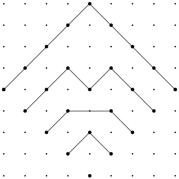
For and , let denote the disjoint -collection described as follows: the path consists of ascents, one flat step, and descents. For , the path consists of ascents, one descent, one ascent, and descents. For and , the path consists of ascents followed by descents. (See Figure 1.)
It is not hard to show that
Moreover,
where the parameter ranges are chosen so that this is a disjoint union. We therefore have that
| (21) |
By considering only which descents in are not in , and vice versa, we find that
Acknowledgements
This research was partially supported by Collaboration Grant #315593 from the Simons Foundation. The author thanks Tom Leinster and Simon Willerton for useful conversations, and the anonymous referee for suggestions which improved the exposition of this paper.
References
- [1] J. A. Barceló and A. Carbery. On the magnitudes of compact sets in Euclidean spaces. Amer. J. Math., 140:449–494, 2018.
- [2] S. Chevet. Processus Gaussiens et volumes mixtes. Z. Wahrscheinlichkeitstheorie und Verw. Gebiete, 36(1):47–65, 1976.
- [3] S. Cho. Quantales, persistence, and magnitude homology. Preprint, available at https://arXiv.org/abs/1910.02905, 2019.
- [4] R. M. Dudley. The sizes of compact subsets of Hilbert space and continuity of Gaussian processes. J. Functional Analysis, 1:290–330, 1967.
- [5] C.-G. Esseen. On mean central limit theorems. Kungl. Tekn. Högsk. Handl. Stockholm, 121:31 pp, 1958.
- [6] H. Gimperlein and M. Goffeng. On the magnitude function of domains in Euclidean space. Preprint, available at https://arxiv.org/abs/1706.06839, 2017.
- [7] H. Gimperlein and M. Goffeng. On the magnitude function of domains in Euclidean space, III: Questions and examples from a geometric analyst’s perspective (a). Blog post at https://golem.ph.utexas.edu/category/2019/01/on_the_magnitude_function_of_d_2.html, 23 January 2019.
- [8] M. Goffeng. Personal communication. 2018.
- [9] L. Goldstein. bounds in normal approximation. Ann. Probab., 35(5):1888–1930, 2007.
- [10] M. Gromov. Metric Structures for Riemannian and Non-Riemannian Spaces. Birkhäuser, Boston, 2001.
- [11] M. Henk and M. A. Hernández Cifre. Intrinsic volumes and successive radii. J. Math. Anal. Appl., 343(2):733–742, 2008.
- [12] R. Hepworth. Magnitude cohomology. Preprint, available at https://arxiv.org/abs/1807.06832, 2018.
- [13] R. Hepworth and S. Willerton. Categorifying the magnitude of a graph. Homology, Homotopy, and Applications, 19(2):31–60, 2017.
- [14] R. A. Horn and C. R. Johnson. Matrix Analysis. Cambridge University Press, Cambridge, second edition, 2013.
- [15] T. Leinster. Integral geometry for the -norm. Advances in Applied Mathematics, 49:81–96, 2012.
- [16] T. Leinster. The magnitude of metric spaces. Doc. Math., 18:857–905, 2013.
- [17] T. Leinster. The magnitude of a graph. Math. Proc. Camb. Phil. Soc., 166:247–264, 2019.
- [18] T. Leinster and M. W. Meckes. Maximizing diversity in biology and beyond. Entropy, 18(3):88, 2016.
- [19] T. Leinster and M. W. Meckes. The magnitude of a metric space: from category theory to geometric measure theory. In Measure Theory in Non-Smooth Spaces, Partial Differ. Equ. Meas. Theory, pages 156–193. De Gruyter Open, Warsaw, 2017.
- [20] T. Leinster and M. Shulman. Magnitude homology of enriched categories and metric spaces. Preprint, available at https://arxiv.org/abs/1711.00802, 2017.
- [21] T. Leinster and S. Willerton. On the asymptotic magnitude of subsets of Euclidean space. Geom. Dedicata, 164:287–310, 2013.
- [22] P. McMullen. Inequalities between intrinsic volumes. Monatsh. Math., 111(1):47–53, 1991.
- [23] M. W. Meckes. Positive definite metric spaces. Positivity, 17(3):733–757, 2013.
- [24] M. W. Meckes. Magnitude, diversity, capacities, and dimensions of metric spaces. Potential Anal., 42(2):549–572, 2015.
- [25] N. Otter. Magnitude meets persistence. Homology theories for filtered simplicial sets. Preprint, available at https://arxiv.org/abs/1807.01540, 2018.
- [26] R. Schneider and W. Weil. Stochastic and Integral Geometry. Probability and its Applications (New York). Springer-Verlag, Berlin, 2008.
- [27] A. R. Solow and S. Polasky. Measuring biological diversity. Environmental and Ecological Statistics, 1:95–107, 1994.
- [28] B. S. Tsirelson. A geometric approach to maximum likelihood estimation for an infinite-dimensional Gaussian location. II. Teor. Veroyatnost. i Primenen., 30(4):772–779, 1985.
- [29] R. A. Vitale. On the Gaussian representation of intrinsic volumes. Statist. Probab. Lett., 78(10):1246–1249, 2008.
- [30] R. A. Vitale. Convex bodies and Gaussian processes. Image Anal. Stereol., 29(1):13–18, 2010.
- [31] S. Willerton. The magnitude of odd balls via Hankel determinants of reverse Bessel polynomials. Preprint, available at https://arxiv.org/abs/1708.03227, 2017.
- [32] S. Willerton. Personal communication. 2018.