Geometry of bounded critical phenomena

Abstract

The quest for a satisfactory understanding of systems at criticality in dimensions $d>2$ is a major field of research. We devise here a geometric description of bounded systems at criticality in any dimension $d$. This is achieved by altering the flat metric with a space dependent scale factor $\gamma(x)$, $x$ belonging to a bounded domain $\Omega$. $\gamma(x)$ is chosen in order to have a scalar curvature to be constant and matching the one of the hyperbolic space, the proper notion of curvature being – as called in the mathematics literature – the fractional Q-curvature. The equation for $\gamma(x)$ is found to be the Fractional Yamabe Equation (to be solved in $\Omega$) that, in absence of anomalous dimension, reduces to the usual Yamabe Equation in the same domain. From the scale factor $\gamma(x)$ we obtain novel predictions for the scaling form of one-point order parameter correlation functions. A (necessary) virtue of the proposed approach is that it encodes and allows to naturally retrieve the purely geometric content of two-dimensional boundary conformal field theory. From the critical magnetization profile in presence of boundaries one can extract the scaling dimension of the order parameter, $\Delta_{\phi}$. For the 3D Ising model we find $\Delta_{\phi}=0.518142(8)$ which favorably compares (at the fifth decimal place) with the state-of-the-art estimate. A nontrivial prediction is the structure of two-point spin-spin correlators at criticality. They should depend on the fractional Q-hyperbolic distance calculated from the metric, in turn depending only on the shape of the bounded domain and on $\Delta_{\phi}$. Numerical simulations of the 3D Ising model on a slab geometry are found to be in agreement with such predictions.

1 Introduction

The understanding of critical phenomena and critical states is a central theme of modern physics. In the course of the study of criticality powerful tools have been developed such as the Renormalization Group able to enlighten universal physical properties from condensed matter systems to high energy physics.

A basic concept that has emerged as a defining property of the critical state is that of being scale invariant. We refrain from working out these concepts in full generality [1] while concentrating on the case of a bounded system defined in a domain $\Omega$ topologically equivalent to a ball. It is well known that, at criticality, for a wide range of systems [1, 2] one can adopt a continuum description where the physical observables depend on the spatial coordinate, in our case $x\in\Omega\subset\mathbb{R}^{d}$. Consider a (space dependent) observable depending on the local degrees of freedom $s(x)$ located inside the domain, think of the order parameter $\phi(x)=s(x)$ as a guiding example. In the critical state the system will have a given distribution of the microscopic degrees of freedom allowing to obtain averages that will be denoted by $\langle\ldots\rangle$. If the system admits a well defined thermodynamic limit the averages are expected to converge to some well behaved function $\langle\phi(x)\rangle$.

The consideration of bounded systems has both practical and theoretical advantages. On the practical side when dealing with real systems (be them experimental or numerical realizations) we are in general treating finite systems. On the theoretical side boundary theories are often more constraining leading to more refined results, moreover corrections to the infinite system system behavior contain information on some fundamental properties of the theory such as the central charge [3, 4]. These relations allow us to access these fundamental quantities even in finite systems.

Scaling hypothesis for the operators implies that if we take a system $\lambda\Omega$ of a size $\lambda$ times larger than $\Omega$ then the correlation function of operator $\phi$ will be given by:

$$\langle\phi(\lambda x)\rangle_{{}_{\lambda\Omega}}=\lambda^{-\Delta_{\phi}}\langle\phi(x)\rangle_{{}_{\Omega}}$$ (1)

where $\Delta_{\phi}$ is the scaling dimension of the field $\phi$ [1, 5]. Similar Ansätze can be put forward for observables depending on more points.

2 Uniformisation

We now put forward our main working hypothesis (Uniformisation):

A system at criticality in a bounded domain will try to modify its (flat euclidean) metric in order to be “as uniform as possible”.

Making the above statement precise and derive from it quantitative, testable nontrivial predictions that will be checked constitutes the aim of the present work. The flat metric will be denoted by $\delta=\delta_{ij}$ where the indices $i$ and $j$ run from $1$ to $d$; the symbol $g$ will instead be reserved for a generic metric $g=g_{ij}$. The allowed change in the metric will be of the type $\delta\rightarrow\delta/\gamma(x)^{2}$ where $\gamma(x)$ is a space dependent scale factor. A reason for allowing changes of this type is that on short scales, such that the effect of boundaries is negligible, the system should locally behave as a bulk system which is isotropic. Such a change in the metric is known in the mathematical literature as a conformal change and metrics related by these transformations are said to belong to the same conformal class.

Since we are trying to set up an intrinsic geometry, the uniformisation should entail curvatures. As we are aiming at fixing one space dependent function $\gamma(x)$ we will have to put constraints on a quantity. A first reasonable guess (which will be later modified) is the scalar curvature, $R_{g}$, where we explicitly noted the dependence on the metric $g$. For convenience we remind how (a normalised version of) $R_{g}$ is defined in terms of the metric $g_{ij}$:

$$\Gamma_{jk}^{i} =\frac{1}{2}g^{il}\left(\partial_{k}g_{lj}+\partial_{j}g_{lk}-\partial_{l}g_{jk}\right)$$ (2)

$$\mathrm{Ric}_{ij} =\partial_{l}{\Gamma^{l}_{ji}}-\partial_{j}\Gamma^{l}_{li}+\Gamma^{l}_{l\lambda}\Gamma^{\lambda}_{ji}-\Gamma^{l}_{j\lambda}\Gamma^{\lambda}_{li}$$ (3)

$$R_{g} =\frac{1}{d(d-1)}\mathrm{Ric}_{ij}g^{ji}$$ (4)

(as usual, summation over repeated indices is assumed).

Thus, according to uniformisation, we would end up with the equation:

$$R_{\delta/\gamma(x)^{2}}=\kappa.$$ (5)

Actually for two-dimensional systems this guess, implementing our uniformisation hypothesis, appears to be well motivated since scalar curvature alone is a quantity fully specifying geometric properties [6]. Now it comes to the choice of the right constant value $\kappa$ to set for $R$. We have the following possibilities:

• $\kappa>0$ is constant positive curvature, think of the sphere $\mathbb{S}^{d}$ as a (very special) example, which does not appear to be suited to describe a system with boundary since it has no borders.

• $\kappa=0$ is a flat space (actually the one we started with) which is also not suited to pursue Uniformisation since the points living near the boundary cannot be treated on the same footing as the other points in the bulk.

• $\kappa<0$ is constant negative curvature, think of the hyperbolic space $\mathbb{H}^{d}$ as a (again very special) example, indeed appears as a reasonable since it is endowed with an infinitely distant boundary.

Since one can always rescale $\kappa$, from now on we choose $\kappa=-1$.

Writing down the equation requires the knowledge of the transformation laws of scalar curvature under conformal changes of the metric. We have that $R_{g/\gamma(x)^{2}}=R_{g}-|\nabla\gamma(x)|^{2}+\frac{2}{d}\gamma(x)\Delta\gamma(x)$. The problem we have just stated is known as the Yamabe problem [7]. Since the $g$ we are starting from is flat ($R_{g}=0$) and we are requiring $R_{g/\gamma(x)^{2}}=\kappa=-1$ , we are aiming at the solution of:

$$1-|\nabla\gamma(x)|^{2}+\frac{2}{d}\gamma(x)\Delta\gamma(x)=0,$$ (6)

i.e. the so-called Yamabe Equation. In (6) gradient and Laplacian are calculated with the flat metric and the function $\gamma$ should be zero on $\partial\Omega$, the boundary of $\Omega$. The Yamabe problem, an old acquaintance to geometers, is the subject of extensive mathematical research in the literature at the interface of analysis and geometry [8, 9, 10]. The Yamabe Equation for $d=2$ has been studied in connection with the Liouville field theory [11] and for $d>2$ it just occasionally surfaced in the physics literature [12, 13].

Another more suggestive form of the above equation is written as the nonlinear eigenvalue problem for the positive definite operator $(-\Delta)$: for $d\neq 2$

$$(-\Delta)\gamma(x)^{-\frac{d-2}{2}}=-\frac{d(d-2)}{4}\gamma(x)^{-\frac{d+2}{2}}.$$ (7)

For $d=2$ a limit has to be performed yielding the Liouville equation

$$(-\Delta)\log\gamma(x)=-\kappa\gamma(x)^{-2}.$$ (8)

In $d=2$ the solution of the above problem inside a (connected and simply connected) domain $\Omega$ amounts exactly to the construction of a model of hyperbolic space $\mathbb{H}^{2}$.

We quote two simple solutions of (7) valid in any $d$: putting $x=(x_{1},x_{2},$ $\ldots,x_{d})$, we have i) for the upper half hyper-space, $x_{d}>0$, it is $\gamma(x)=x_{d}$; ii) for a ball of radius $r$ we have $\gamma(x)=\frac{r^{2}-x^{2}}{2r}$ where $x^{2}=\sum_{i=1}^{d}x_{i}^{2}$ . These two are examples where by conformally altering the metric we can construct $\mathbb{H}^{d}$, i.e. a space where not only $R$ but all the sectional curvatures are constant. The two-dimensional case stands on its own because as already mentioned $R$ is enough to specify the geometric properties of the space. The spaces constructed inside say a disk and a square will be isometric and the coordinate change between them will be the conformal mapping between the interiors of the square and the disk (so in this case a Schwarz-Christoffel mapping) that due to Riemann mapping theorem exists, provided the domains are regular enough.

But let’s pursue the geometric reasoning. Having obtained a uniformising metric, we wish to construct from it predictions for observables. The obtained metric indeed constitutes, locally, a gauge for measuring lengths. One-point correlators should be function of it. Let us now inspect how the solution of the Yamabe Equation changes under a rescaling of the domain. We have that

$$\gamma_{{}_{\lambda\Omega}}(\lambda x)=\lambda\gamma_{{}_{\Omega}}(x).$$ (9)

Given this transformation law, based on our uniformisation hypothesis, we are led to conjecture that:

$$\langle\phi(x)\rangle=const.\times\gamma(x)^{-\Delta_{\phi}},$$ (10)

where $\gamma$ is the solution of Yamabe Equation (6). We anticipate that in (10) we are not fully taking into account the effect of anomalous dimension on the metric; this will be fixed in the next two Sections.

We now turn to two-point correlators. For the two-point correlator $\langle\phi(x)\phi(y)\rangle$, a prefactor $\gamma(x)^{-\Delta_{\phi}}\gamma(y)^{-\Delta_{\phi}}$ restoring the correct physical dimensions is expected, while what is missing, because of our hypothesis of a purely geometric description, should be only a function $F$ of the distance $\mathfrak{D}_{\delta/\gamma^{2}}(x,y)$ between points $x$ and $y$, calculated with the metric $\delta/\gamma^{2}$. This yields:

$$\langle\phi(x)\phi(y)\rangle=\gamma(x)^{-\Delta_{\phi}}\gamma(y)^{-\Delta_{\phi}}F(\mathfrak{D}_{\delta/\gamma^{2}}(x,y)).$$ (11)

The above considerations can be extended for higher order correlators. For example three-point functions should contain three dimensional prefactors and an arbitrary function of three mutual distances and so on.

What we have just outlined is indeed true for two-dimensional systems and, with $d>2$, for systems defined in the upper half hyperspace or inside a hypersphere as derived by using the group of conformal symmetries [14]. In $d=2$, for one-point functions it coincides with known results in bounded critical systems, see e.g. [15, 16, 17, 18], while, always in $d=2$, for higher point correlators it matches the transformation law for correlators in boundary conformal field theories (see e.g. 5.24 in [3]) under conformal mappings. From our geometric viewpoint this is traced back to the fact that all complete, connected, simply-connected spaces of constant negative scalar curvature are isometric in two dimensions.

In order to see explicitly in $d>2$ that our results agrees with symmetry-based derivations [14], recall that for the $d$-dimensional upper half hyperspace the hyperbolic distance is $\mathfrak{D}_{\delta/x_{d}^{2}}(x,y)=\mathrm{arccosh}\left[1+\frac{|x-y|_{d-1}^{2}+(x_{d}-y_{d})^{2}}{2x_{d}y_{d}}\right]$ where $|x-y|_{d-1}^{2}=\sum_{i=1}^{d-1}(x_{i}-y_{i})^{2}$. Our conjecture for two-points then exactly reproduces what can be found in formula (3.9) of [14]. We stress that this is special to the upper half hyperspace and inside a hypersphere domains that do not acquire a dependence on anomalous dimension. Our results refer instead to any domain in any dimension. For domains different from the upper half space and the ball the anomalous dimension plays a role in $d>2$, as we discuss in the next Section.

We remark another rewarding property of the structure of solutions of Yamabe problem: close to the boundary of $\Omega$, as it can be gleaned from (6), we have that $\gamma(x)$ is proportional to the euclidean distance to the boundary $\partial\Omega$. This implies a locality property: near the boundary the system effectively looks like a hyperbolic space forgetting about the detailed shape of the domain. This feature is also retained by solutions of the fractional Yamabe problem that will shortly be introduced.

The explicit analytical solution for the Yamabe Equation in a slab domain relevant for the interpretation of numerical experiments is presented in Appendix A.

3 Anomalous dimensions inclusion

The content of this section is not meant to give a microscopic derivation of our main results, expressed by (24)-(25), but to provide qualitative arguments to support and motivate the conjectures that will be stated in Section 4 and verified in Section 5.

Let us reconsider the Yamabe Equation in a different light. Take a general theory which is at most quadratic in the fields. Its action is given by:

$$\mathcal{S}[\phi(x)]=\int\mathrm{d}^{d}x\frac{1}{2}\phi(x)(A\phi)(x)-\int\mathrm{d}^{d}xb(x)\phi(x),$$ (12)

where $A$ is a general linear operator which should be positive in order to ensure control over fluctuations of the field. A good example is obviously minus the Laplacian, $A=(-\Delta)$. $b(x)$ is an external magnetic field. With this action we can perform averages as follows:

$$\langle\phi(x^{\prime})\phi(x^{\prime\prime})\phi(x^{\prime\prime\prime})\ldots\rangle_{Q}=\frac{1}{\mathcal{Z}}\int\mathcal{D}[\phi(x)](\phi(x^{\prime})\phi(x^{\prime\prime})\phi(x^{\prime\prime\prime})\ldots)\exp(-\mathcal{S}[\phi(x)])$$ (13)

with the normalization $\mathcal{Z}=\int\mathcal{D}[\phi(x)]\exp(-\mathcal{S}[\phi(x)])$. We can calculate the average of the order parameter obtaining

$$\langle\phi(x)\rangle_{Q}=A^{-1}b(x)$$ (14)

where the inverse of $A$ has appeared. Inverting the above relation we get

$$A\langle\phi(x)\rangle_{Q}=b(x).$$ (15)

Let us now take $A=(-\Delta)$ and pursue some geometric considerations based on scaling. Assume there is a metric, $\gamma_{Q}(x)$, describing the system at criticality. The field $\phi$ has scaling dimensions $\frac{d-2}{2}$, also known as free field or canonical dimensions, while $b(x)$ will have scaling dimensions $\frac{d+2}{2}$ for the action to be dimensionless [1, 2]. With these assumptions Eq. (15) reads:

$$(-\Delta)\gamma_{Q}(x)^{-\frac{d-2}{2}}=const.\times\gamma_{Q}(x)^{-\frac{d+2}{2}}$$ (16)

and it has reproduced the Yamabe Equation. We stress again that this is not meant to be a rigorous derivation, but a way to obtain equations with correct dimensional properties.

Let us now exploit and insert some common knowledge we have from the theory of critical phenomena. A generic observable will have some scaling dimension differing from the free field one. The presence of so-called anomalous dimensions is at the heart of the existence of a nontrivial theory of critical phenomena. As an example take the magnetization in the 3D Ising model which has a scaling dimension of $\Delta^{CB}_{\phi}=0.5181489(10)$ [19]. We quote the best result to date obtained via the Conformal Bootstrap technique [19], other high precision determinations of $\Delta_{\phi}$ are to be found in [20, 21, 22, 23] and are reported in Table 1 presented in Section 5. This result differs by a small, but definitely nonzero amount from the expected canonical dimension $\frac{d-2}{2}=\frac{1}{2}$.

How can we correct the above equations to account for the anomalous scaling? A first guess would be to simply substitute the order parameter with $\gamma(x)^{-\Delta_{\phi}}$ and the conjugate field with $\gamma(x)^{-d+\Delta_{\phi}}$. However the Laplacian would have the wrong scaling dimensions. A natural way out is to consider a power of it:

$$(-\Delta)^{\frac{d}{2}-\Delta_{\phi}}\left[\gamma_{(\Delta_{\phi})}(x)\right]^{-\Delta_{\phi}}=const.\times\left[\gamma_{(\Delta_{\phi})}(x)\right]^{-d+\Delta_{\phi}},$$ (17)

where the subscript ${}_{(\Delta_{\phi})}$ on $\gamma$ signals the dependence on the anomalous dimension $\Delta_{\phi}$. Eq. (17) is the so-called Fractional Yamabe Equation. It emerged in the context of the fractional Yamabe problem, i.e. finding metrics making generalizations of the scalar curvature, the so-called fractional $Q$-curvatures, constant. The first definition of this problem with rigorous results for the case of compact manifolds appeared in [24].

We remind that in the full space $\mathbb{R}^{d}$ (with no boundaries) several definitions of the fractional Laplacian are known in literature [25, 10] and they do coincide [26]. However Equation (17) is to be solved in the bounded domain $\Omega$. When adapted to bounded domains, the different definitions of the fractional Laplacian in general do not any longer coincide and this is both a problem for applications and a challenge for mathematical research which is currently subject of intense work [27].

For the purposes of the present paper we anyway need to define and solve Equation (17) in bounded domains. This has to be done in order to compare the results with lattice Monte Carlo simulations to validate our Uniformisation hypothesis and the conjectures, that will be stated in the following Equations (24)-(25), for one-point and two-point correlations.

The route we follow to overcome these difficulties is to introduce a conformally covariant version of the fractional Laplacian in bounded domains, as detailed in the next section.

For later convenience we introduce $s$, the order of the fractional Laplacian:

$$s=\frac{d}{2}-\Delta_{\phi}.$$

4 Conformally covariant formulation

While the derived equations (7) and its generalisation (17) make sense, their appearance is not so satisfying since they depend on operators defined in the reference (flat) space. It would be very appealing to have operators transforming in a consistent way under conformal changes of the metric. Actually it is much more than an aesthetic consideration, since to have good conformal transformation properties is a quite strong requirement for the construction of a fractional Laplacian.

On a manifold $M$ of dimension $d$ (this definition is usual for compact manifolds, while we shall need it in the non-compact case), we define an operator $A_{g}$ to be conformally covariant if under a conformal change in the metric $g\rightarrow g^{\prime}=g/w^{2}$ ($w(x)$ being an arbitrary positive gauge function) the relation

$$A_{g^{\prime}}(w^{p}\varphi)=w^{q}A_{g}(\varphi)$$ (18)

holds, where $\varphi$ is a function in $C^{\infty}(M)$ and $p$ and $q$ are constants. Notably the operator

$$\mathcal{L}^{(1)}_{g}=(-\Delta_{g})+\frac{d(d-2)}{4}R_{g},$$ (19)

called the conformal Laplacian, falls under this classification with $p=\frac{d-2}{2}$ and $q=\frac{d+2}{2}$, being $-\Delta_{g}$ the Laplace-Beltrami operator for the metric $g$ and $R_{g}$ its scalar curvature as defined in (4). With this operator the Yamabe Equation transforms into

$$\mathcal{L}^{(1)}_{\delta/{w(x)^{2}}}\left(\frac{\gamma(x)}{w(x)}\right)^{-\frac{d-2}{2}}=-\frac{d(d-2)}{4}\left(\frac{\gamma(x)}{w(x)}\right)^{-\frac{d+2}{2}}$$ (20)

and takes an especially simple form if we write it in terms of the metric $\delta/\gamma(x)^{2}$:

$$\mathcal{L}^{(1)}_{\delta/\gamma(x)^{2}}(\mathbbm{1})=-\frac{d(d-2)}{4}(\mathbbm{1}).$$ (21)

This means that the metric uniformising scalar curvature is the one which acting with its associated conformal Laplacian on a constant field (denoted by $\mathbbm{1}$) brings it to (a multiple of) the constant field, making in some sense its uniformising properties more explicit. Of course the numerical difficulties of solving the equation are still there.

Other operators (not general enough for this work) are the conformally covariant integer powers of the Laplacian: the Paneitz operator [28] and the GJMS operators [29]. Most important are instead scattering operators first defined in [30] for compact manifolds whose definition has been reconciled with more conventional definitions of the fractional Laplacian in [31].

In terms of the properly defined fractional Laplacian $\mathcal{L}^{(s)}_{g}$ of order $s$, Fractional Yamabe Equation reads:

$$\mathcal{L}^{(\frac{d}{2}-\Delta_{\phi})}_{\delta/w^{2}}\left(\frac{\gamma_{(\Delta_{\phi})}(x)}{w(x)}\right)^{-\Delta_{\phi}}=\frac{\Upsilon(\Delta_{\phi})}{\Upsilon(d-\Delta_{\phi})}\left(\frac{\gamma_{(\Delta_{\phi})}(x)}{w(x)}\right)^{-d+\Delta_{\phi}}.$$ (22)

Again choosing $w(x)^{2}=\gamma_{(\Delta_{\phi})}(x)^{2}$ one has

$$\mathcal{L}^{(\frac{d}{2}-\Delta_{\phi})}_{\delta/\gamma_{(\Delta_{\phi})}^{2}}(\mathbbm{1})=\frac{\Upsilon(\Delta_{\phi})}{\Upsilon(d-\Delta_{\phi})}(\mathbbm{1}),$$ (23)

where the dependence on $\Delta_{\phi}$ of $\gamma$ has been explicitly noted. With this notation the solution of Yamabe Equation is $\gamma_{(\frac{d-2}{2})}(x)$. The constant has been fixed in terms of the function ${\Upsilon(x)\equiv\Gamma(1-x)\,\sin(\pi x/2)}$ such that the hyperbolic space $\mathbb{H}^{d}$ is a solution, proof of this statement and calculation of the constant are to be found in Appendix B. The two conjectures stated in the previous Section, Equations (10)-(11), stay the same, but with the anomalous dimension dependent scale factor $\gamma_{(\Delta_{\phi})}(x)$. Thus we can put forward the following

Conjecture for one-point correlators:

$$\langle\phi(x)\rangle=const.\times\left[\gamma_{(\Delta_{\phi})}(x)\right]^{-\Delta_{\phi}},$$ (24)

and

Conjecture for two-point correlators:

$$\langle\phi(x)\phi(y)\rangle=\left[\gamma_{(\Delta_{\phi})}(x)\right]^{-\Delta_{\phi}}\left[\gamma_{(\Delta_{\phi})}(y)\right]^{-\Delta_{\phi}}F(\mathfrak{D}_{\delta/{\gamma_{(\Delta_{\phi})}}^{2}}(x,y)).$$ (25)

Remember that $\mathfrak{D}_{g}(x,y)$ is the distance calculated with the metric $g$ and $\gamma_{(\Delta_{\phi})}(x)$ is the solution of Equation (23).

Equations (24) and (25) are the main results of this paper, and we emphasize they are intended to be valid in any bounded domain at criticality in any dimension. We expect similar formulas to hold for higher-point correlators.

Predictions from (24)-(25) will be checked against numerical simulations for the Ising model in a non-trivial domain, the slab, in the next Section. Notice that if one, unlike our approach, assumes at criticality just an effective theory having only fractional derivatives in the kinetic term (and no interaction terms), one would face in a bounded domain the following two inherent problems: first one would be forced to choose which definition of the fractional Laplacian has to be used, and moreover the structure of the different correlators would obey unavoidably Wick theorem, leaving no freedom for higher-point correlators.

Equipped with the operator $\mathcal{L}^{(s)}$, we can write down an expression for the fractional Q-curvature, $R_{g}^{(s)}$, for a generic metric $g$:

$$R_{g}^{(s)}=-\frac{\Upsilon\left(\frac{d}{2}+s\right)}{\Upsilon\left(\frac{d}{2}-s\right)}\mathcal{L}^{(s)}_{g}\left(\mathbbm{1}\right)$$ (26)

where the coefficient in front of the rhs is chosen in order to have the fractional Q-curvature to be minus one for $\mathbb{H}^{d}$. In order to not interrupt the flow of the presentation, we give in the Appendices B-C the details needed for the formal construction of the fractional Laplacian $\mathcal{L}^{(s)}_{g}$ in a bounded domain and the numerical solution of the Fractional Yamabe Equation (23) in the slab geometry. The construction relies on considering the $d$-dimensional domain $\Omega$ as the boundary of a suitably defined $d+1$ dimensional space [32]. The obtained findings will be compared with lattice Monte Carlo simulations in the same geometry.

5 Comparison with numerical experiments

In order to test our predictions we will consider the fruit fly of statistical mechanics: the Ising model [2]. We perform Monte Carlo simulations on a slab geometry, where the value of the spins is fixed to the value $1$ on the two planes delimiting the slab. The model is simulated at the critical temperature. The value of the magnetization in this geometry only depends on the distance from the planes, and we record as well the two-point correlation functions. The profile of the magnetization near boundary at criticality for the Ising model and many other statistical mechanics models has been thoroughly investigated in the literature of boundary critical phenomena [33]. In particular the boundary conditions we are using correspond to the so-called extraordinary phase transitions [33]. In the thermodynamic limit the magnetization has to be rescaled by multiplying it by $L^{\Delta_{\phi}}$ yielding – at criticality – a universal scaling function [14]. A crucial step to reduce finite size effects is to introduce the extrapolation length $a$ [34], accounting for the expected power-law divergence not occurring exactly at the boundary in the lattice system. Collapse of numerical data can be used this way to obtain estimates of $\Delta_{\phi}$ [34], but the resulting value for it is not especially precise. Much better Monte Carlo estimates for $\Delta_{\phi}$ are rather obtained by analyzing data with cross correlations between various thermodynamic quantities [23] or determining by finite size scaling the value of parameters where leading corrections to scaling vanish [22], however reaching to date a significantly smaller precision than the Conformal Bootstrap estimates [19]. A summary of the best results for $\Delta_{\phi}$ is in Table 1 together with our new estimate, obtained as follows.

Our determination is based on the knowledge of the solution $\gamma_{(\Delta_{\phi})}$ of the Fractional Yamabe Equation for the slab geometry. In accordance with our conjecture (24) for one-point operators we have $\langle\phi(x)\rangle\propto\left[\gamma_{(\Delta_{\phi})}(x)\right]^{-\Delta_{\phi}}$. Denoting by $i$ the lattice coordinate in the transverse direction of the slab, $i=0,\ldots L$, we compute from Monte Carlo simulation the magnetization $m_{i}=\langle s_{i}\rangle=\langle\phi(x)\rangle$ where $s_{i}$ is the discrete Ising variable and $x=\frac{2i}{L}-1$ so that $x\in[-1,1]$.

We then fit the magnetization data using:

$$m_{i}=\alpha L^{-\Delta_{\phi}}\left[\gamma_{(\Delta_{\phi})}\left(\frac{x}{1+a/L}\right)\right]^{-\Delta_{\phi}},$$ (27)

where the parameters $a$, $\alpha$, and $\Delta_{\phi}$ are left free. Since we want to determine $\Delta_{\phi}$ in an unbiased fashion (not relying on previous estimates) the function $\gamma_{(\Delta_{\phi})}(x)$ has to be determined for a range a values, that is chosen to be $[0.5,0.54]$. In Appendix C, Figure 4 a contour plot of this function is reported. We see to our surprise that the dependence on $\Delta_{\phi}$ around the free field value $\Delta_{\phi}=0.5$ is pretty weak.

To obtain accurate results it is important to minimize fine size corrections to scaling. Because of universality, we are free to choose a model within the same universality class. Such a model has already been devised [22] and used to obtain the most refined Monte Carlo numerical results. It is the improved Blume-Capel model (at criticality), whose Hamiltonian is reported in Appendix D together with details of the simulations. In order to assess the validity of our predictions the magnetization has been measured and compared with our conjecture. The results for the magnetization are reported in Figure 1, where we also show the collapse of the data.

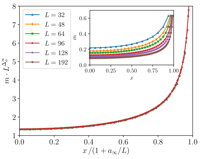
Figure 1: Collapse plot of the magnetization data for the different sizes considered. The parameters used, $a_{\infty}$, $\alpha_{\infty}$, $\Delta_{\phi}^{\infty}$, are the ones extrapolated for $L=\infty$. The red line is the universal scaling function $\alpha_{\infty}\left[\gamma_{(\Delta_{\phi}^{\infty})}(x)\right]^{-\Delta_{\phi}^{\infty}}$ for the magnetization. The inset displays the raw data obtained from the simulations. In all cases the errors are smaller than the size of the points.

Details of the fitting procedure are in Appendix E. The results for $\Delta_{\phi}$ are plotted in Figure 2. The obtained estimates are close to the best Conformal Bootstap result available so far $\Delta_{\phi}^{CB}$ [19], and the $L=192$ value, $\Delta_{\phi}=0.518150(22)$, is extremely close to it. Since the data are all compatible with each other for $L\geq 64$, we are allowed to perform a weighted average of them yielding the value $\Delta_{\phi}=0.518142(8)$. This value is compatible with $\Delta_{\phi}^{CB}$ and it has an order of magnitude larger error. In turn it is more precise, by an order of magnitude than the best MC estimates reported in the literature [22, 23]. All these results are summarised in Table 1 with our estimate denoted by “Critical Geometry” for brevity.

In Table 2 we report the values obtained for the different sizes in two ways. In the central column we use the metric $\gamma_{(\Delta_{\phi})}$ obtained by solving the Fractional Yamabe Equation with a $\Delta_{\phi}$ which is left free and extracted from the fit of numerical results. In the right column we report the values obtained using the non-fractional Yamabe profile raised to a power $\Delta_{\phi}$ left free. On one side one can observe that the latter values obtained from the Yamabe Equation are not accurate as much as the ones reported in the central column when compared with the best Conformal Bootstrap value $\Delta_{\phi}^{CB}$. On the other side the Yamabe Equation value is anyway rather good. The reason for this (somehow unexpected) result is the already mentioned weak dependence of the solution of the Fractional Yamabe Equation on the anomalous dimension, signaling the rigidity of the hyperbolic spaces whatever constant curvature is imposed. The anomalous dimension contribution to the metric factor is however important to get highly accurate estimates for $\Delta_{\phi}$. Anyway, we consider the fact that the non-fractional Yamabe Equation produces good results as a confirmation of the reliability of our geometrical approach. Therefore we expect that for more complicated domain shapes, where the solution of the Fractional Yamabe Equation may be very difficult to find, one could use the integer Yamabe Equation as a first good approximation.

Reference	Method	$\qquad\Delta_{\phi}$
Hasenbusch (2010) [22]	MC	0.518135(50)
Ferrenberg et al. (2018) [23]	MC	0.51801(35)
Sheer El-Showk et al. (2014) [21]	Conformal Bootstrap	0.518154(15)
Kos et al. (2016) [19]	Conformal Bootstrap	0.5181489(10)
This paper	Critical Geometry	0.518142(8)

Table 1: Best results for the 3D Ising scaling exponent of the order parameter $\Delta_{\phi}$. The best results to our knowledge to date for $\Delta_{\phi}$ are contained in lines 1 and 4 pertaining to MC and Conformal Bootstrap method respectively. The last line is the value obtained using the approach described in this paper and denoted as “Critical Geometry”.

Linear size $L$	$\Delta_{\phi}$ FYE profile fit	$\Delta_{\phi}$ YE profile fit
32	0.52287(24)	0.52570(17)
48	0.51955(21)	0.52200(15)
64	0.51812(13)	0.52038(7)
96	0.51812(7)	0.51983(3)
128	0.51811(5)	0.51931(3)
192	0.518150(22)	0.518923(15)

Table 2: Size dependent fitting values for $\Delta_{\phi}$ using (central column) the Fractional Yamabe Equation (FYE) profile and (right column) the ordinary Yamabe Equation (YE) profile for different values of the linear size $L$ (left column).

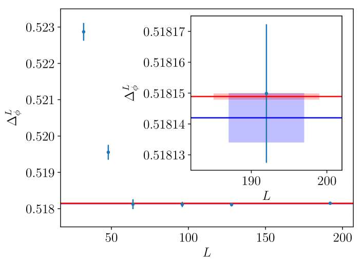
Figure 2: Estimated values of $\Delta_{\phi}^{L}$ for the simulated sizes. The horizontal blue line represents our best estimate $\Delta_{\phi}^{\infty}$, while the red line is $\Delta_{\phi}^{CB}$ [19]. The inset is a zoom for the largest size. In the main figure the error $\Delta_{\phi}^{CB}$ is reported as a shade. In the inset as well errors are represented as shades, however the shades are broken in order to better appreciate the overlap between the estimates.

As for two-point correlators are concerned we evaluate the ratio:

$$r(x,y)=\frac{\langle\phi(x)\phi(y)\rangle}{\langle\phi(x)\rangle\langle\phi(y)\rangle},$$ (28)

and we plot it against the distance $\mathfrak{D}_{\delta/{\gamma_{(\Delta_{\phi}^{CB})}}^{2}}(x,y)$ calculated with the metric corresponding to $\Delta_{\phi}^{CB}$ checking whether a collapse of data points occurs as predicted by our conjecture (25). This is done in Figure 3. The collapse is visibly good and it gets better as the system size is increased from $L=64$ to $L=128$ with the outliers moving towards the collapse line. This has been assessed quantitatively by calculating a root mean square of deviations $\bar{\chi}$ from a fitting function that actually halves as the size is doubled. In Appendix E details of the analysis of the two-point correlation functions are reported toghether with collapse performed with other metrics.

While the data coming from two-point correlators fully comply with our conjecture, the achieved precision does not allow to rule out a geometric description based on non-fractional Yamabe distance (i.e. the one based on the solution of Yamabe Equation), that yields a very similar collapse plot. Again, we consider this effectiveness of the description with the Yamabe Equation as a signature of the robustness of the devised geometric approach presented in this paper.

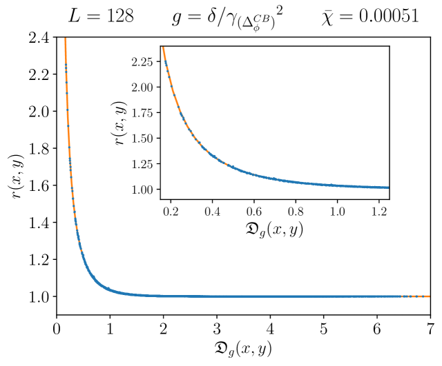
Figure 3: Correlation ratio $r(x,y)$ defined in Equation (28) in terms of distances $\mathfrak{D}$ calculated with the solution of Fractional Yamabe Equation $\gamma_{(\Delta_{\phi}^{CB})}$ for the two system sizes $L=64$ and $L=128$. The value of $\bar{\chi}$ is reported in the upper right corner of the figures. The continuous line is a fitting function as reported in Appendix E.

6 Future directions

The present work aims at giving a unified description of the geometrical content of bounded critical phenomena. When applied to two-dimensional systems, it allows to retrieve from a different perspective known results of boundary conformal field theory in $d=2$ [18]. For higher dimensions new predictions for physically relevant observables were derived. For the 3D Ising model the comparison between numerical results and the predictions of the theory developed here is encouraging and it motivates further efforts along these lines.

We stress that the achieved description is purely geometric in the sense that it depends on the considered bounded domain $\Omega$ and on the dimension $d$ independently from the specific model that one is studying on the domain – save for the anomalous dimension $\Delta_{\phi}$, which at variance does depend on the model. The scaling exponents belong instead to the dynamical, model dependent, content of the theory. One of the advantages of our approach, and in essence its main feature, is to cleanly separate geometry/kinematics from dynamics/interaction. In the well studied case of two dimensions the former is simple: since there is no dependence on $\Delta_{\phi}$ for $\gamma(x)$, one geometry fits all models. More precisely, the metric rendering ordinary scalar curvature constant and negative makes also the fractional Q-curvature constant washing away the $\Delta_{\phi}$ dependence, which is not the case for $d>2$. In $d=2$ the information about dynamics is contained in and can be extracted from the further structure of the Virasoro algebra. In this respect many questions are still open.

How different scaling operators other than the order parameter and belonging to the same model may have different geometries, i.e. different scale factors? How do the different geometries combine to give a consistent unified framework? Most likely the answer to these questions will lie in the close examination of short distance properties of higher-point correlation functions in the so-called operator product expansion which is at the very heart of the Conformal Bootstrap approach. In this light it would be very important the comparison of the approach presented here for the energy operator with numerical simulations in the Ising model.

Moreover it would be highly desiderable to enlarge the number of models, shape of bounded domains and boundary conditions on which our predictions are tested in 3D and higher. A natural candidate would be the XY model that however displays a scaling dimension not differing much from the canonical one. Currently work is being pursued in this direction by looking at multicritical points with different discrete symmetry groups that appear to have larger deviations from the canonical dimensions [35]. Very promising is also the study of percolation models in $d>2$ with the techniques presented in [36]. A boundary condition to be considered is the free boundary condition pertaining to the so-called ordinary boundary transition. In addition to considering homogeneous boundary condition it would be useful to consider also different boundary conditions in the same model. These concepts, well developed in the two-dimensional world (see [37, 38] for recent applications), are central to modern topics such as SLE that are still lacking a higher-dimensional counterpart.

We point out that the prediction for one-point and two-point correlators in a bounded domain are based on the solution of a fractional conformally covariant differential equation in the same domain. To sensibly define the fractional Laplacian in the bounded domain with the boundary conditions imposed by criticality, one has to view the domain as the boundary of an asymptotically hyperbolic space living in one more dimension. This approach shares some traits with the AdS/CFT correspondence. It would be interesting to investigate the relations between the geometric approach to criticality developed here and the formulation of statistical mechanics models at criticality with AdS/CFT techniques.

This work builds a theory for critical phenomena deeply rooted in geometry. Is there an algebraic counterpart to it? This is to be intended as a “critical Langlands program”. Current work is being pursued by inspecting the structure of infinitesimal deformations of the bounded domain in which Fractional Yamabe Equation is studied.

Appendix A Solution of the Yamabe Equation for the slab domain

Here we report the solution of Yamabe Equation for the slab domain in arbitrary dimension $d$ being defined as $-1<x=x_{1}<1$ and $x_{i}\in\mathbb{R}$ for $i=2,\ldots,d$. The equation for $\gamma(x)$ becomes a nonlinear ordinary differential equation:

$$1-(\partial_{x}\gamma)^{2}+\frac{2}{d}\gamma\partial_{x}^{2}\gamma=0.$$ (29)

The solution satisfying the appropriate boundary conditions $\gamma(\pm 1)=0$ can be given in terms of the inverse function $x(\gamma)$

$$\pm x(\gamma)=1-\phantom{}_{2}F_{1}\left(\frac{1}{2},\frac{1}{d};1+\frac{1}{d};(\gamma/\gamma_{0})^{d}\right)\gamma,$$ (30)

where the signs refer to the two symmetric with respect to $x\rightarrow-x$ branches and $\gamma_{0}=\gamma(0)$ is the ($d$-dependent) metric factor on the symmetry plane $x=0$ of the slab:

$$\gamma_{0}=\frac{\Gamma\left(\frac{1}{2}+\frac{1}{d}\right)}{\sqrt{\pi}\,\Gamma\left(1+\frac{1}{d}\right)}.$$ (31)

$\gamma(x)$ can be explicitly obtained in selected cases: the (trivial) one-dimensional case $\gamma_{d=1}(x)=\frac{1-x^{2}}{2}$, the two-dimensional (strip) case $\gamma_{d=2}(x)=\frac{2}{\pi}\cos\left(\frac{\pi x}{2}\right)$ while in the $d\rightarrow\infty$ limit $\gamma_{d\rightarrow\infty}(x)=1-|x|$. In figure 4 we depict $\gamma_{d}(x)$ for $d=3$, relevant for the subsequent analysis, and $d=2$ for comparison.

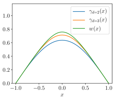
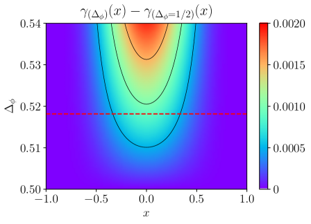
Figure 4: (Left) Solution of Yamabe problem in the strip ($d=2$) and slab ($d=3$) domain. The additional function $w(x)$ is the gauge function used to solve Fractional Yamabe Equation for the slab domain. (Right) Solutions of the Fractional Yamabe Equation as $\Delta_{\phi}$ is varied in the range $[0.5,0.54]$. The plot actually shows deviations from the $\Delta_{\phi}=1/2$ Yamabe solution (the $d=3$ curve in the left panel). The red dashed line is the Conformal Bootstrap value $\Delta_{\phi}^{CB}$ [19].

Appendix B Scattering operators for bounded domains

A complete discussion of the presented approach, including thorough mathematical justification, will be given in [32].

A way to construct the operators with the required conformal properties is the following. Consider the domain $\Omega$ equipped with the metric $g$ to be the boundary of a higher dimensional $d+1$ manifold, call it $X$ having a metric $g_{+}$. Denoting the extra coordinate with $y$, we pose that our original domain $\Omega$ is retrieved when we set $y=0$ and be regular $\mathrm{d}y|_{\Omega}\neq 0$. A coordinate $y$ with such properties is called a defining function. Moreover near $\Omega$ the metric $g_{+}$ should look like $g_{+}\approx g/y^{2}$ making our space $(X,g_{+})$ asymptotically a hyperbolic space. This surface will be called the conformal infinity. The metric space $(X,g_{+})$ should be an Einstein space, that is it has to satisfy vacuum Einstein field equations $\mathrm{Ric}(g_{+})+d\,g_{+}=0$, where $\mathrm{Ric}$ is the Ricci tensor in the $d+1$ dimensional space.

Given a function $f_{I}$ on $\Omega$ solve the following eigenvalue problem for the function $U$ (defined over $X$):

$$\begin{cases}&(-\Delta_{g_{+}})U=\Delta_{\phi}(d-\Delta_{\phi})U\\ &U=y^{\Delta_{\phi}}F_{I}+y^{d-\Delta_{\phi}}F_{O},\end{cases}$$ (32)

where $\Delta_{g_{+}}$ is the Laplacian for the metric $g_{+}$, $F_{I}$ and $F_{O}$ are regular functions (the subscripts $I$ and $O$ stand for input and output respectively) as $y$ approaches zero and $F_{I}|_{y=0}=f_{I}$. The requirement of $(X,g_{+})$ to be Einstein guarantees the existence of a solution of the above equation (special care has to be taken when $d-\Delta_{\phi}$ differs from $\Delta_{\phi}$ by an integer where a resonance condition is met and log terms have to be included in the expansion).

The conformal fractional Laplacian of the function $f_{I}$ can be read off from the boundary behavior of $f_{O}=F_{O}|_{y=0}$. Indeed we have that $\mathcal{L}^{(s)}_{g}f_{I}=c_{s}f_{O}$ where $c_{s}=2^{2s}\frac{\Gamma(s)}{\Gamma(-s)}$. The good transformation properties under conformal changes of this operator can be seen by choosing a different defining function, call it $\upsilon$. As the eigenvector $U$ will be unchanged we have that

$$U=y^{\Delta_{\phi}}F_{I}+y^{d-\Delta_{\phi}}F_{O}=\upsilon^{\Delta_{\phi}}F_{I}^{\prime}+\upsilon^{d-\Delta_{\phi}}F_{O}^{\prime}$$ (33)

where $F_{I}^{\prime}$ and $F_{O}^{\prime}$ are respectively input and output data of another scattering problem. Since around the conformal infinity the two defining function are linearly related, $y=\left.\frac{dy}{d\upsilon}\right|_{\Omega}\upsilon=w(x)^{-1}\upsilon$, we obtain the desired transformation law:

$$g\rightarrow w(x)^{-2}g,f_{I}\rightarrow w(x)^{\Delta_{\phi}}f_{I},f_{O}\rightarrow w(x)^{d-\Delta_{\phi}}f_{O}.$$ (34)

The above method first presented in [30] has to be adapted to the case of bounded domains. In this case the extension metric space $(X,g_{+})$ has to fulfill additional properties dealing with boundaries of $\Omega$, and it should be a so-called cornered asymptotic hyperbolic space [39]. There an additional surface emerges $\omega$ detached from $\Omega$ and sharing the same boundary $\partial\Omega=\partial\omega$. The surface $\omega$ should be totally geodesic, that is, geodesics restricted to $\omega$ should coincide with geodesics in $X$. Heuristically this can be understood as a decoupling of what happens inside $X$ from what happens beyond $\omega$, which acts as an invisible wall. This construction can always be performed, as shown in [39], provided $\partial\Omega$ is regular enough, and the metric $g_{+}$ can be put in the canonical form:

$$g_{+}=(\sin\theta)^{-2}(d\theta^{2}+g_{\theta}),$$ (35)

where the extension variable $\theta$ plays the role of an incidence angle at the conformal infinity and $g_{\theta=0}=g$. In these convenient variables the manifold $X$ is $[0,\pi/2]\times\Omega$ where $\theta=0$ is the surface $\Omega$ and $\theta=\pi/2$ is the totally geodesic surface $\omega$. The full set of equations for the metric becomes:

$$\begin{cases}\mathrm{Ric}(g_{+})+d\,g_{+}=0\\ \partial_{\theta}g_{\theta}|_{\theta=\pi/2}=0\\ g_{\theta}^{-1}|_{[0,\pi]\times\partial\Omega}\rightarrow 0\end{cases}$$ (36)

supplemented by the regularity of $g_{\theta}$ for $\theta=0$. A cartoon of the space $X$ is represented in Figure 5. As for the extension problem the additional natural boundary conditions on $U$ are vanishing normal derivative $\partial_{\mathbf{n}}U|_{\partial X\setminus(\Omega\cup\omega)}=0$ and also $\partial_{\theta}U|_{\partial\omega}=0$. With the boundary conditions described we have a good candidate for a Neumann conformally covariant fractional Laplacian.

Figure 5: Depiction of the extension space $X$. The planes represent constant $\theta$ hypersurfaces. The points joined by dotted lines should be identified. The red lines are geodesics with endpoints on the depicted hypersurfaces. The bottom hypersurface is the conformal infinity, the central hypersurface is the totally geodesic surface, and the upper hyperplane is the complement of the conformal infinity.

We now provide an example where the fractional Laplacian can be calculated and where we verify that the hyperbolic metric indeed solves the non-compact fractional Yamabe problem. Consider the upper half hyperspace $\mathbb{R}_{+}^{d}$ in $d$ dimensions and view it as the boundary of the space $X=[0,\pi/2]\times\mathbb{R}_{+}^{d}$; the extension coordinate being $\theta$. The metric

$$g_{+}=(\sin\theta)^{-2}(d\theta^{2}+g_{\theta})=(\sin\theta)^{-2}(d\theta^{2}+dx^{2}/x_{d}^{2})$$ (37)

satisfies the (cornered) Einstein vacuum equation (36). If we plug in the function

$$U=\tau^{\Delta_{\phi}}\eta(\Delta_{\phi},\tau)+\frac{\tau^{d-\Delta_{\phi}}}{c_{s}}\frac{\Upsilon(\Delta_{\phi})}{\Upsilon(d-\Delta_{\phi})}\eta(d-\Delta_{\phi},\tau),$$ (38)

where $\tau=\tan(\theta)$ and $\eta(\Delta_{\phi},\tau)={}_{2}F_{1}(\frac{\Delta_{\phi}}{2},\frac{1+\Delta_{\phi}}{2};1-\frac{d}{2}+\Delta_{\phi};-\tau^{2})$, we see that the scattering problem is actually satisfied with the correct boundary conditions. What we have just described proves that

$$\mathcal{L}^{(\frac{d}{2}-\Delta_{\phi})}_{\delta/x_{d}^{2}}(\mathbbm{1})=\frac{\Upsilon(\Delta_{\phi})}{\Upsilon(d-\Delta_{\phi})}(\mathbbm{1}),$$

meaning that the hyperbolic metric in $\mathbb{R}_{+}^{d}$ has constant fractional Q-curvature $R_{\delta/x_{d}^{2}}^{(\frac{d}{2}-\Delta_{\phi})}=-1$ (cfr. Equation (26)). The performed computation for $d=2$ can be adapted to any regular enough domain via a conformal mapping viewed as an isometry between models of the hyperbolic plane. For $d>2$ it allows to retrieve the metric factor just for the hyperball domain which is the only one isometric to the hyperbolic space. For other domains we will have to proceed as specified in the next Appendix.

Appendix C Spectral solution of the Fractional Yamabe Equation in the slab geometry

Further details of this solution will also be presented in [32]. Before defining the conformal fractional Laplacian for the slab domain a solution to Einstein Equations has to be found. For the slab case the metric can be put in the canonical form (35) with a diagonal metric:

$$g_{+}=(\sin\theta)^{-2}\left[d\theta^{2}+dx^{2}/\gamma_{x}(x,\theta)^{2}+(dx_{2}^{2}+dx_{3}^{2})/\gamma_{\parallel}(x,\theta)^{2}\right]$$ (39)

(remember that $x=x_{1}\in[-1,1]$ denotes the transverse direction of the slab). With this Anstatz a solution of (36) has been found. In Figure 6 the functions $\gamma_{x}(x,\theta)$ and $\gamma_{\parallel}(x,\theta)$ are shown. On the conformal infinity $\theta=0$ they do by construction coincide, thus providing a good metric to calculate conformally invariant Laplacians in the flat conformal class. The function $\gamma_{x}(x,0)=\gamma_{\parallel}(x,0)=w(x)$ shown in Figure 4 will specify the actual gauge in which computations will be performed.

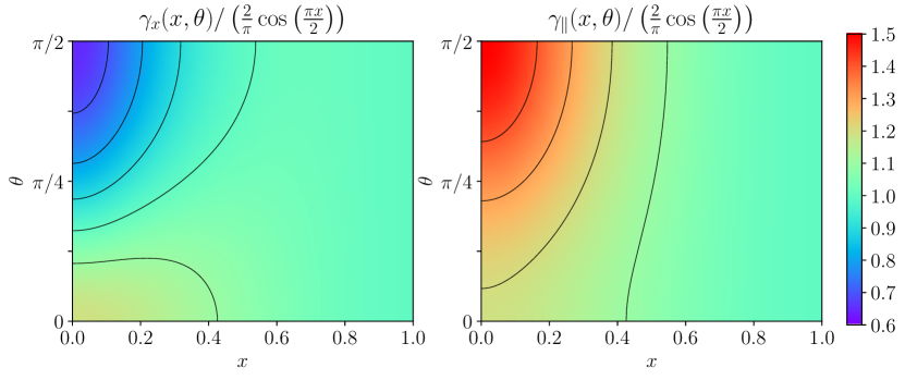
Figure 6: Solution of Einstein equations as specified by the functions $\gamma_{x}(x,\theta)$ and $\gamma_{\parallel}(x,\theta)$ in the extension space above the slab. The domain shown is $x\in[0,1]$ and $\theta\in[0,\pi/2]$. The regions $x\in[-1,0]$ and $\theta\in[\pi/2,\pi]$ can be obtained by reflection. To improve readability, the functions have been divided by $\frac{2}{\pi}\cos\left(\frac{\pi x}{2}\right)$.

Because of the outlined structure of the solution of the extension problem near the conformal infinity, the following form will be assumed for $U$:

$$U =\sin(\theta)^{\Delta_{\phi}}u=$$

$$=\sin(\theta)^{\Delta_{\phi}}\left(\sum_{i=0,\,i\,\mathrm{even}}^{N_{\theta}}\mathcal{F}_{i}(x)\sin(\theta)^{2i}+\sum_{i=1,\,i\,\mathrm{odd}}^{N_{\theta}}\mathcal{F}_{i}(x)\sin(\theta)^{2s+i-1}\right).$$ (40)

The function $\mathcal{F}_{i}(x)$ are even functions that will be represented as linear combinations of $N_{x}$ even Chebyshev polynomials $T_{2j}(x)$:

$$\mathcal{F}_{i}(x)=\sum_{j=0}^{N_{x}}T_{2j}(x)\psi_{i,j}.$$ (41)

The extension partial differential equation problem will be evaluated on a set of $N_{\theta}\times N_{x}$ collocation Gauss-Lobatto points given by $\theta_{i}=\frac{\pi}{2}\left[1-\cos\left(\frac{\pi i}{2N_{\theta}}\right)\right]$, $x_{j}=\cos\left(\frac{\pi j}{2N_{x}}\right)$ with $i=1,\ldots,N_{\theta}$ and $j=1,\ldots,N_{x}$, reducing it to a solution of a matrix equation. The boundary conditions are given by $\partial_{x}u=0$ on $x=\pm 1$ and $\partial_{\theta}u=0$ on $\theta=\pi/2$. The input data (the function of which we are calculating the fractional Laplacian) is given by the $\mathcal{F}_{0}(x)$, while the output (the fractional Laplacian) is given by $\mathcal{L}^{(s)}_{\delta/w^{2}}[\mathcal{F}_{0}](x)=c_{s}\mathcal{F}_{1}(x)$.

Let us turn to the nonlinear eigenvalue problem contained in (23). By numerical experimentation, the framework proves more stable if we work with the inverse of the fractional Laplacian $\mathcal{I}=\frac{\Upsilon(\Delta_{\phi})}{\Upsilon(d-\Delta_{\phi})}[\mathcal{L}^{(s)}_{\delta/w^{2}}]^{-1}$. The form we have actually considered is:

$$\mathcal{E}[\rho]=\mathcal{I}[\rho]-\rho^{\frac{\Delta_{\phi}}{d-\Delta_{\phi}}}=0,$$ (42)

where $\rho=\left(\gamma/w\right)^{-d+\Delta_{\phi}}$. The above equation has been solved by looking for a minimum of $\sum_{j=0}^{N_{x}}|\mathcal{E}[\rho](x_{j})|^{2}$. This minimisation yields, in a stable way, a very small value (on the order of $10^{-24}$) signaling that the equation is satisfied to a very high accuracy. The chosen collocation grid for the numerical solution is $N_{x}=N_{\theta}=20$. Since the values of $\Delta_{\phi}$ of interest to us are around $\Delta_{\phi}\approx 0.52$, we solved the Fractional Yamabe Equation on a Gauss-Lobatto grid of $12$ values in $(0.5,0.54]$ allowing us to obtain reliable solutions for the fractional Yamabe problem in the slab in this range via Chebyshev interpolation. The solutions turn out to differ only slightly from the solution of Yamabe Equation and connect smoothly to it when $\Delta_{\phi}\rightarrow 1/2$ (that is $s\rightarrow 1$). The deviations from the Yamabe Equation solution for the slab domain are shown in the right panel of Figure 4.

Appendix D Monte Carlo experiments

The model we simulate has the Hamiltonian:

$$\mathcal{H}=-\beta\sum_{<i,j>}s_{i}s_{j}+D\sum_{i}s_{i}^{2},$$ (43)

where the spins $s_{i}$ are located on a cubic lattice $i=(i_{1},i_{2},i_{3})$ and assume the three values $s_{i}=-1,0,1$. $<i,j>$ denote nearest neighbors. The parameters take the values $\beta=0.387721735$ and $D=0.655$ for the system to be at the critical point in their current best estimates [22]. We expect that, going to larger systems, more precise determination of the critical point will be in order. The geometry we consider is a three-dimensional slab, with $0\leq i_{1}\leq L$ and $0\leq i_{2},i_{3}\leq L_{\parallel}$. $L$ should be made larger and larger (lattice spacing is set to one). Of course we will be simulating a finite system approximating the specified geometry. The transverse direction will have $L+1$ sites (out of which $L-1$ will be left free to vary) and the parallel ones $L_{\parallel}$ sites with periodic boundary conditions along the parallel directions. The boundary sites in the transverse direction will be fixed to one. This boundary condition, known as extraordinary, is imposed in order to develop a nonzero order parameter. In order to make the finiteness of the parallel directions less relevant, but the system size still tractable, we will choose $L_{\parallel}=6L$which we checked to be large enough to cancel the dependence on $L_{\parallel}$ in the measured observables. The sizes considered are $L=32,48,64,96,128,192$ reaching a maximum of $191\cdot 1152^{2}\approx 2.5\cdot 10^{8}$ free sites. We expect that in order to perform simulations for larger sizes would require a more precise determination of the critical parameters with respect to the ones in [22]. The algorithm used is the one described in [34]. Moreover, in order to reduce statistical fluctuations an analytical variance reduction technique has been used similarly to what done in [40] in a numerical way: it amounts to summing over states of the spin under consideration and its nearest neighbors exactly.

The number of samples collected after a suitably long thermalisation stage of $10^{4}$ MC steps is on the order of $10^{6}$ samples. Of course autocorrelation reduces the number of independent samples. This has been dealt with by blocking techniques [41].

Appendix E Data analysis

The variance reduced one-point data have been averaged along parallel directions to reduce statistical fluctuations. The fitting procedure with function (27) has been adapted to the raw data in the following way. The points in the center of the slab are more sensitive to the functional form of the universal scaling function which however has a rather generic parabolic shape. The points near the boundary on the other side, while allowing for direct access to the critical exponents, are more affected by finite size effects. In order to get the most out of our data a weighting window function has been applied to the data: it is one in the slab center, decays linearly with a width of two sites and it is zero beyond that point. The position of this window has been adapted in a continuous way such that our theory is consistent with a $p$-value of $95\%$. These are the data reported in Table 2. The required windowing becomes smaller and smaller as the size is increased with the center of the linear part of the window being located at $x\simeq 0.9$ for the largest size $L=192$. We remark that if a similar analysis is carried out with the, not theoretically justified but anyway seemingly sensible, magnetization profile for the strip $\gamma_{d=2}(x)^{-\Delta_{\phi}}$ the data yield the incorrect estimate for $\Delta_{\phi}\simeq 0.8$ with a heavy windowing of the data keeping only the central half of the points. This clearly rules out the description with $\gamma_{d=2}$.

As for two-point data, we recorded the spin-spin correlation functions for all the possible distinct pairs $(i,j)$ of points in the following set: $i_{1}=m_{1}(L/16)$, $i_{2}=0$, $i_{3}=0$ and $i_{1}=n_{1}(L/16)$, $i_{2}=n_{2}(L/16)$, $i_{3}=n_{3}(L/16)$ with $m_{1},n_{1}=1,\ldots,15$ and $n_{2},n_{3}=0,\ldots,14$. This yields a total of $7672$ independent correlators since coinciding points have been excluded and pairs symmetric under reflection have been put together. Average over parallel directions has obviously been performed. For these measurements the data set is approximately $10$ times smaller than the one collected for one-point functions.

For each of these couple of points the distance has been calculated and plotted against ratio (28). In order to see how a collapse can go wrong let us check a case where it should not work from the outset. While rotational symmetry is broken we may nonetheless plot as a check our ratio against euclidean distance: this yields, as expected, the very poor collapse shown in Figure 7. For the (more difficult to handle) metric $\delta/\gamma_{(\Delta_{\phi})}^{2}$ the calculation of the distances has been performed numerically taking advantage of the geodesics functionality present in the program Surface Evolver [42]. In order to assess the goodness of the collapse, we fit $r$ as a function of $\mathfrak{D}_{g}$ with the function $f(x)=1+\sum_{i=1}^{3}a_{i}e^{-b_{i}x}$. This yields a reasonable description of the data that will be taken with no errors since they are much smaller than the observed spread. The figure of merit will be the root mean square of deviations from the fitting function:

$$\bar{\chi}=\sqrt{\frac{\left[r-f(\mathfrak{D}_{g})\right]^{2}}{n_{\mathrm{d.o.f.}}}},$$ (44)

where $n_{\mathrm{d.o.f.}}=7666$ is the number of degrees of freedom. Let us see quantitatively whether a collapse occurs with the, already ruled out by one-point correlator analysis, strip metric factor $\gamma_{d=2}$. Results are shown in Figure 8. While yielding a reasonable collapse, we remark that points with $\mathfrak{D}\simeq 1$ have a considerable spread and, more importantly the value of $\bar{\chi}$ increases with the system size, ruling out again $\gamma_{d=2}$ as the correct metric factor.

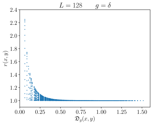
Figure 7: Correlation ratio $r(x,y)$ defined in Eq. (28) in terms of the euclidean distance $\mathfrak{D}_{\delta}$ for $L=128$.

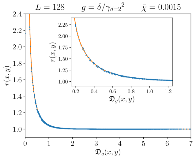
Figure 8: Correlation ratio $r(x,y)$ in terms of distances $\mathfrak{D}$ calculated with the strip distance $\gamma_{d=2}=\left(\frac{2}{\pi}\right)\cos\left(\frac{\pi x}{2}\right)$ for the two system sizes $L=64$ and $L=128$. The value of $\bar{\chi}$ is also reported. The continuous line is the fitting function $f$, see text for details.

References

- [1] Cardy, John L.; “Scaling and Renormalization in Statistical Physics”, Cambridge University Press (1996).
- [2] Mussardo, Giuseppe; “Statistical Field Theory”, Oxford University Press (2010).
- [3] Di Francesco, Philippe; Mathieu, Pierre; Sénéchal, David; “Conformal Field Theory”, Springer (1997).
- [4] Blöte, H. W. J.; Cardy, John L.; and Nightingale, M. P.; “Conformal invariance, the central charge, and universal finite-size amplitudes at criticality”, Phys. Rev. Lett. 56, 742 (1986).
- [5] Fisher, Michael E.; De Gennes, P. G.; “Wall phenomena in a critical binary mixture”. Comptes rendus hebdomadaires des séances de l’Académie des sciences. Série B 287, 207 (1978).
- [6] do Carmo, Manfredo P.; “Differential geometry of curves and surfaces”, Prentice-Hall, Inc., Englewood Cliffs, N.J. (1976).
- [7] Yamabe, Hidehiko; “On a deformation of Riemannian structures on compact manifolds”, Osaka Journal of Mathematics 12, 21 (1960).
- [8] Schoen, Richard; “Conformal deformation of a Riemannian metric to constant scalar curvature”, J. Differential Geom. 20, 479 (1984).
- [9] Lee, John Marshall; Parker, Thomas H.; “The Yamabe problem”, Bulletin of the American Mathematical Society 17, 37 (1987).
-
[10]
González, María del Mar; “Recent progress on the fractional Laplacian in conformal geometry”,
arXiv:1609.08988, Chapter in “Recent Developments in Nonlocal Theory”, Berlin, Boston: Sciendo Migration. Palatucci, G.; Kuusi, T.; (Eds.) (2018). - [11] Zamolodchikov, A.; Zamolodchikov, Al.; “Conformal bootstrap in Liouville field theory”, Nuclear Physics B 477, 577 (1996).
- [12] Kiessling, Michael K.-H.; “Statistical mechanics approach to some problems in conformal geometry. Statistical mechanics: from rigorous results to applications”, Physica A: Statistical Mechanics and its Applications 279 353 (2000).
- [13] Kholodenko, Arkady L.; Ballard, Ethan E.; “From Ginzburg-Landau to Hilbert-Einstein via Yamabe”, Physica A: Statistical Mechanics and its Applications 380, 115 (2007).
- [14] Cardy, John L.; “Conformal invariance and surface critical behavior”, Nuclear Physics B 240, 514 (1984).
- [15] Cardy, John L.; “Universal Critical-Point Amplitudes in Parallel-Plate Geometries”, Phys. Rev. Lett. 65, 1443 (1990).
- [16] Burkhardt, Theodore W.; Xue, Tianyou; “Density profiles in confined critical systems and conformal invariance”, Phys. Rev. Lett. 66, 895 (1991).
- [17] Reš, Ivica; Straley, Joseph P.; “Order parameter for two-dimensional critical systems with boundaries”, Phys. Rev. B 61, 14425 (2001).
-
[18]
Cardy, John L.; “Boundary conformal field theory”,
arXiv:hep-th/0411189, in Encyclopedia of Mathematical Physics, Elsevier (2006). - [19] Kos, Filip; Poland, David; Simmons-Duffin, David; Vichi, Alessandro; “Precision Islands in the Ising and O(N) Models”, J. High Energy Phys. 2016, 36 (2016).
- [20] El-Showk, Sheer; Paulos, Miguel F.; Poland, David; Rychkov, Slava; Simmons-Duffin, David; Vichi, Alessandro; “Solving the 3D Ising model with the conformal bootstrap”, Phys. Rev. D 86, 025022 (2012).
- [21] El-Showk, Sheer; Paulos, Miguel F.; Poland, David; Rychkov, Slava; Simmons-Duffin, David; Vichi, Alessandro; “Solving the 3d Ising Model with the Conformal Bootstrap II. -Minimization and Precise Critical Exponents”, Journal of Statistical Physics. 157, Issue 4–5, 869 (2014).
- [22] Hasenbusch, Martin; “Finite size scaling study of lattice models in the three-dimensional Ising universality class”, Phys. Rev. B 82, 174433 (2010).
- [23] Ferrenberg, Alan M.; Xu, Jiahao; Landau, David P.; “Pushing the Limits of Monte Carlo Simulations for the 3d Ising Model”, Phys. Rev. E 97, 043301 (2018).
- [24] González, María del Mar; Qing, Jie; “Fractional conformal Laplacians and fractional Yamabe problems”, Anal. & PDE 6, Number 7, 1535 (2013).
- [25] Pozrikidis, Constantine; “The Fractional Laplacian”, CRC Press, Boca Raton, (2016).
- [26] Kwaśnicki, Mateusz; “Ten equivalent definitions of the fractional Laplace operator”, Fract. Calc. Appl. Anal. 20, Number 1, 7 (2017).
- [27] Lischke, Anna et al.; “What Is the Fractional Laplacian? A comparative review with new results”, J. Comput. Phys. 404, 109009 (2020).
- [28] Branson, Thomas; “An anomaly associated with -dimensional quantum gravity”, Comm. Math. Phys. 178, Number 2, 301 (1996).
- [29] Graham, Robin C.; Jenne, Ralph; Mason, Lionel J.; Sparling, George A. J.; “Conformally invariant powers of the Laplacian, I: Existence”, Journal of the London Mathematical Society 2, 557 (1992).
- [30] Graham, Robin C.; Zworski, Maciej; “Scattering matrix in conformal geometry”, Inventiones mathematicae 152, 89 (2003).
- [31] Chang, Sun-Yung Alice; González, María del Mar; “Fractional Laplacian in conformal geometry”, Advances in Mathematics 226, 1410 (2011).
- [32] González, María del Mar; Gori, Giacomo; Graham, Robin C.; Saez, Mariel; in preparation.
- [33] Diehl, Hans Werner; “The Theory of Boundary Critical Phenomena”, International Journal of Modern Physics B 11, No. 30, 3503 (1997).
- [34] Hasenbusch, Martin; “Thermodynamic Casimir effect for films in the three-dimensional Ising universality class: Symmetry-breaking boundary conditions”, Phys. Rev. B 82, 104425 (2010).
- [35] Ben Alì Zinati, Riccardo; Codello, Alessandro; Gori, Giacomo; “Platonic Field Theories”, J. High Energy Phys. 2019, 152 (2019).
- [36] Gori, Giacomo; Trombettoni, Andrea; “Conformal invariance in three dimensional percolation”, J. Stat. Mech. 2015, P07014 (2015).
- [37] Gori, Giacomo; Viti, Jacopo; “Exact logarithmic four-point functions in the critical two-dimensional Ising model”, Phys. Rev. Lett. 119 191601 (2017).
- [38] Gori, Giacomo; Viti, Jacopo; “Four-point boundary connectivities in critical two-dimensional percolation from conformal invariance”, J. High Energy Phys. 2018 131 (2018).
- [39] McKeown, Stephen E.; “Formal Theory of Cornered Asymptotically Hyperbolic Einstein Metrics”, J. Geom. Anal. 29, 1876 (2019).
- [40] Hasenbusch, Martin; “Two- and three-point functions at criticality: Monte Carlo simulations of the improved three-dimensional Blume-Capel model”, Phys. Rev. E 97, 012119 (2018).
- [41] Efron, Bradley; “Bootstrap methods: Another look at the jackknife”, Ann. Stat. 7, 1 (1979).
- [42] Brakke, Kenneth A.; “The surface evolver”, Experiment. Math. 1, 141 (1992).