Cosmic-ray transport from AMS-02 B/C data: benchmark models and interpretation

Abstract

This article aims at establishing new benchmark scenarios for Galactic cosmic-ray propagation in the GV-TV rigidity range, based on fits to the AMS-02 B/C data with the usine v3.5 propagation code. We employ a new fitting procedure, cautiously taking into account data systematic error correlations in different rigidity bins and considering Solar modulation potential and leading nuclear cross section as nuisance parameters. We delineate specific low, intermediate, and high-rigidity ranges that can be related to both features in the data and peculiar microphysics mechanisms resulting in spectral breaks. We single out a scenario which yields excellent fits to the data and includes all the presumably relevant complexity, the BIG model. This model has two limiting regimes: (i) the SLIM model, a minimal diffusion-only setup, and (ii) the QUAINT model, a convection-reacceleration model where transport is tuned by non-relativistic effects. All models lead to robust predictions in the high-energy regime ($\gtrsim 10$ GV), i.e. independent of the propagation scenario: at $1\sigma$, the diffusion slope $\delta$ is $[0.43-0.53]$, whereas $K_{10}$, the diffusion coefficient at 10 GV, is $[0.26-0.36]$ kpc² Myr^-1; we confirm the robustness of the high-energy break, with a typical value $\Delta_{h}\sim 0.2$. We also find a hint for a similar (reversed) feature at low rigidity around the B/C peak ($\sim 4$ GV) which might be related to some effective damping scale in the magnetic turbulence.

I Introduction

The last decade in direct cosmic-ray (CR) detection experiments has been characterized by a major improvement in the precision of the data available, and by an extension of the covered dynamical range Ahn et al. (2009); Panov et al. (2009); Adriani et al. (2014); Ting (2013); Adriani et al. (2017); Ambrosi et al. (2017). In particular, with the AMS-02 data the community has to deal for the first time with percent level precision and a welcomed redundancy in the measurements.

But, as well known, great responsibility inseparably follows from great power : since theoretical predictions are very far from attaining that level of precision, both due to ignorance of the detailed underlying microphysics (CR acceleration and transport) and because of irreducible limitations (e.g. due to the intrinsic stochasticity of the sources Mertsch (2011); Genolini et al. (2017)), a preliminary question that should be addressed is that of the best strategy to take advantage of such a wealth of data. In this paper, we primarily focus on the AMS-02 B/C data Aguilar et al. (2016) and investigate how much they can constrain CR transport, aiming at defining new benchmark models.

An ambitious approach would be to proceed with global fits of all available data, attempting an overall and simultaneous understanding of CR sources (all species) and propagation. However, this approach is prone to mixing uncertainties of different nature, with the risk of devaluing the actual strength of the data by introducing poorly controlled parameters (for an illustration, see Coste et al. (2012)). Since our current understanding of CR measurements has more firm elements in the propagation part than in the source one, factorizing out propagation effects from source effects, while inspecting their physical plausibility a posteriori, seems justified. In this article, we proceed through partial tests of key aspects of the current propagation paradigm, with the goal of validating it or highlighting its breakdown. An important and relatively new issue in this area is that systematic errors are often dominant over statistical ones. This requires a change of perspective in well-established practices of analyzing the data, as well as new standards of rigor. It calls for establishing a satisfactory protocol for analyzing the data on a relatively simple and homogeneous data sample.

This article represents an important pillar in our CR data analysis based on the overall philosophy sketched above. As long established Owens (1976); Ginzburg et al. (1980); Protheroe et al. (1981); Strong and Moskalenko (1998); Maurin et al. (2001), a flux ratio of elements present but in traces in the solar system material and interstellar medium (ISM), such as Lithium, Beryllium, Boron (“secondaries”), to abundant species like Carbon or Oxygen (“primaries”) is extremely sensitive to propagation parameters. It was shown to be also almost insensitive to the energy spectrum of the injected primary species, notably if those are described by a common power-law in rigidity Maurin et al. (2002a); Putze et al. (2011); Genolini et al. (2015), a rather generic prediction of studies of CR acceleration at sources Malkov and Drury (2001); Caprioli and Spitkovsky (2014); Amato (2014); Marcowith et al. (2016). In particular, at high rigidities we expect the B/C ratio (currently the most precisely measured) to be dominantly affected by diffusive propagation and nuclear cross sections.

In Génolini et al. (2017), we performed an analysis of the high-rigidity range of the AMS-02 B/C ratio Aguilar et al. (2016), finding evidence for a diffusive origin of the observed spectral break, at the same rigidity scale inferred from a similar feature in the proton and helium CR fluxes Aguilar et al. (2015), i.e. $\sim 300$ GV. Actually, recent years have been characterized by the observational establishment of “spectral anomalies” (for reviews, see Serpico (2015, 2018)), in particular of spectral breaks in primary species Panov et al. (2009); Ahn et al. (2010); Adriani et al. (2011); Aguilar et al. (2015, 2015, 2017). In turn, there has been growing evidence in favor of their interpretation in terms of a high-rigidity break in the diffusion coefficient (Génolini et al., 2017; Reinert and Winkler, 2018; Xue and Niu, 2019), notably after the first AMS-02 publications of nuclear CR fluxes Aguilar et al. (2017, 2018). In this article, we move several steps beyond our previous analysis Génolini et al. (2017), presenting a complete analysis aiming at constraining CR propagation and at proposing new benchmark setups: First, we rely on an improved analysis of the B/C data by the AMS-02 collaboration Aguilar et al. (2018). We further benefit from additional data on the primary species to constrain the break independently from the B/C ratio—using the C and O fluxes Aguilar et al. (2017) which are most contributing species to B production Génolini et al. (2018), but were not available to Ref. Génolini et al. (2017). Second, we follow the new methodology proposed in Derome et al. (2019) to analyze the AMS-02 data, carefully accounting for a number of subtle (but highly important) effects which are usually ignored, notably the (partial) correlations in systematic errors. This approach enables a straightforward and sound statistical interpretation of the models (best-fit models have $\chi^{2}/{\rm dof}\sim 1$), also allowing for their inter-comparison. Third, we propose a new generic propagation model (dubbed BIG in the following), with a number of parameters that should be sufficient to describe all key features currently present in the data. In addition to a high-rigidity break, a modification of the diffusion coefficient at low rigidity is enabled ($\lesssim 5$ GV), with two limiting cases (dubbed SLIM and QUAINT): this allows us to assess the relative discriminating strength of the data in this energy range and to shed new light on propagation in the low-rigidity regime, where a second diffusion break might be present.

The paper is organized as follows: In Sect. II, the one-dimensional (1D) propagation model and the essential physical effects involved in CR propagation are presented, before introducing our three benchmark scenarios (BIG, SLIM, and QUAINT). In Sect. III, we describe the specific iterative procedure used for the B/C analysis, and this procedure is validated and checked in two appendices: App. A assesses the robustness of the derivation of the high-energy break, by taking advantage or not of the C and O fluxes; App. B further discusses the dependence of the fit parameters upon the lower rigidity cut, to better illustrate and give meaning to the terms “low-rigidity” and “high-rigidity”parameters. Best-fit results for our three scenarios are presented in Sect. IV, where these scenarios are also tentatively interpreted in terms of the underlying microphysics. In Sect. V, we report our conclusions and mention natural follow-up works. Note that all results are obtained for a 1D model of our Galaxy, with the size of the diffusive halo fixed. In order to allow for a broader usage of our results, as they may have some consequence in predicting the fluxes of other secondary species, App. C provides a scaling of the high-rigidity parameters with $L$, whereas App. D reminds the reader of the effectiveness of this description, and provides a “dictionary” to interpret the results in terms of a two-dimensional (2D) model with different halo sizes.

II Transport models

In this section, we introduce the generic propagation equation that we further solve semi-analytically in the framework of the usine code Maurin (2018) – for fully numerical frameworks complementary to ours, we refer the reader to Refs. Strong and Moskalenko (1998); Evoli et al. (2008, 2017); Kissmann (2014); Kissmann et al. (2015). We also set a generic CR transport configuration motivated by theoretical arguments on the microphysics of CRs, with a focus on possibly important low-energy processes. This generic setup will itself be used as a benchmark configuration, of which we shall explore two limiting regimes. These three cases characterize new benchmark models (dubbed BIG, SLIM, and QUAINT—see Sect. II.2) that are aimed at capturing different theoretical assumptions, while still being data driven. These configurations will be shown to provide excellent fits to the current B/C data assuming simple power-law primary CR spectra. Not only may this stimulate further microphysical interpretations, but it also offers a basis for a description of other CR data, like for instance the positron Delahaye et al. (2009, 2010); Boudaud et al. (2017a) and antiproton fluxes Donato et al. (2001); Giesen et al. (2015); Reinert and Winkler (2018); Boudaud et al. (2019). Eventually, these benchmarks will be instrumental in characterizing and hopefully reducing theoretical uncertainties entering searches for exotic phenomena (e.g. Delahaye et al. (2008); Boudaud et al. (2015a, b, 2017b); Boudaud and Cirelli (2018); Boudaud et al. (2018); Reinert and Winkler (2018)).

The min, med, and max benchmark values proposed in Ref. Donato et al. (2004), all based on the same model, were defined to roughly bracket the theoretical uncertainties on dark matter-induced antiproton flux predictions assuming the best-fitting propagation parameters of Ref. Maurin et al. (2001). However, these values have been challenged by a series of complementary constraints Lavalle et al. (2014); Boudaud et al. (2017a); Reinert and Winkler (2018), and are anyway no longer consistent with the B/C data Génolini et al. (2017). The revised reference models we propose here rely on different assumptions on the microphysics of CR transport instead of different values of parameters within the same configuration. This change in philosophy stems from the fact that with increasing precision in the (multiwavelength and multimessenger) observational data and improvements on the theory side, we expect to arrive soon to a much better understanding and description of the CR microphysics itself than it was possible two decades ago Marcowith et al. (2016); Amato and Blasi (2018).

II.1 Transport description

II.1.1 Transport equation

The general formalism that provides a powerful description of the transport of CRs in the Milky Way derives from the seminal textbook by Ginzburg and Syrovatskii Ginzburg and Syrovatskii (1964) (see also Berezinskii et al. (1990); Schlickeiser (2002)), and relies on the following diffusion-advection equation for a CR species of index $\alpha$, here in the steady-state approximation and in energy space (rather than rigidity or momentum space):

$$-\;\vec{\nabla}_{\bf x}\left\{K(E)\,\vec{\nabla}_{\bf x}\psi_{\alpha}-\vec{V}_{\rm c}\psi_{\alpha}\right\}+\frac{\partial}{\partial E}\left\{b_{\rm tot}(E)\;\psi_{\alpha}-\beta^{2}\,K_{pp}\,\frac{\partial\psi_{\alpha}}{\partial E}\right\}+\sigma_{\alpha}\,v_{\alpha}\,n_{\rm ism}\,\psi_{\alpha}+\Gamma_{\alpha}\,\psi_{\alpha}$$ (1)

$$=\;q_{\alpha}+\sum_{\beta}\left\{\sigma_{\beta\to\alpha}v_{\beta}n_{\rm ism}\,+\Gamma_{\beta\to\alpha}\right\}\,\psi_{\beta}\;.$$

This equation describes the spatial and energy evolution of the differential interstellar CR density per unit energy $\psi_{\alpha}\equiv dn_{\alpha}/dE$, assuming a net primary injection rate of $q_{\alpha}$, and a secondary injection rate arising from inelastic processes converting heavier species of index $\beta$ into $\alpha$ species (with a production rate $\sigma_{\beta\to\alpha}v_{\beta}n_{\rm ism}$ on the ISM density $n_{\rm ism}$, or a decay rate $\Gamma_{\beta\to\alpha}$). This source term is balanced by several other terms, among which the decay rate $\Gamma_{\alpha}$ (if relevant). The central piece of the propagation equation is the spatial diffusion coefficient $K$, that we discuss in more detail in Sect. II.1.3. The other processes are mostly relevant at low rigidity, but may still affect the determination of higher-energy parameters: convection is featured by a velocity $\vec{V}_{\rm c}$, diffusive reacceleration is parameterized by the energy-dependent coefficient $K_{pp}$, and the inelastic destruction rate is given by $\sigma_{\alpha}v_{\alpha}n_{\rm ism}\,\psi_{\alpha}$, with the $\sigma$’s being energy-dependent nuclear cross sections; energy losses are characterized by the rate $b_{\rm tot}\equiv dE/dt$, which includes ionization and Coulomb processes as prescribed in Mannheim and Schlickeiser (1994); Strong and Moskalenko (1998), as well as adiabatic losses induced by convection and reacceleration, see Maurin et al. (2002a); Putze et al. (2010).

Finally, we can switch from the interstellar (IS) CR flux predictions to the top-of-atmosphere (TOA) ones by means of the force-field approximation Gleeson and Axford (1968); Fisk (1971), for which we only indicate the Fisk potential $\phi_{\rm F}$. The latter is constrained from Ref. Ghelfi et al. (2016) for the AMS-02 data taking period.

II.1.2 Geometry and cross sections

We assume a 1D propagation model, as introduced in e.g. Bulanov and Dogel (1974); Ptuskin (1974); Jones (1979); Ptuskin and Soutoul (1990); Jones et al. (2001); Maurin et al. (2001), where the magnetic halo confining the CRs is an infinite slab in the radial direction and of half-height $L$. Indeed, the radial boundary has only a minor quantitative impact on other transport parameters when the diffusion coefficient is taken as a scalar function (see e.g. Maurin et al. (2002a); Putze et al. (2010)), and neglecting the radial dependence allows us to more efficiently probe the entire available parameter space without significant loss of generality. Therefore, we consider the vertical coordinate $z$ to be the only relevant spatial coordinate. See however App. D for some considerations on the correspondence between 1D and 2D models.

The sources of CRs and the ISM gas which they scatter off are taken homogeneous in an infinitely thin disk at $z=0$, with an effective half-height $h=100$ pc. Energy losses are also considered to be localized in the disk, $b_{\rm tot}\propto 2\,h\,\delta(z)$. The ISM density is set to $n_{\rm ism}=2\,h\delta(z)\,n_{0}$, where $n_{0}=1$ cm^-3, corresponding to a surface density of $\Sigma_{\rm ism}=2\,h\,n_{0}\simeq 6\times 10^{20}$ cm^-2 consistent with observations Ferrière (2001). We assign 0.9 and 0.1 of this budget to hydrogen and helium (in number), respectively. We do not indulge here in a more detailed discussion of the determination of these parameters and of their error from independent observations, since they are largely degenerate with the normalization of the diffusion coefficient (see, e.g., Maurin et al. (2010)).

For the nuclear production and spallation cross sections, we use as reference the sets of tables from the Galprop package, while allowing for normalization, energy shift and low-energy slope changes according to the NSS method described in Derome et al. (2019).

II.1.3 Diffusion in real space and momentum space, and convection

An important physical ingredient to all propagation models is the diffusion coefficient, which describes the scattering of CRs off magnetic turbulence. We assume that it can be taken as a scalar function, homogeneous and isotropic all over the magnetic slab. This is likely a good approximation in the context of B/C analyses because the CR flux is locally isotropic and the magnetic field configuration of the Milky Way exhibits relative fluctuations $\delta B/B\sim 1$ over all relevant spatial scales $\lambda$ (or wavenumbers $k=2\pi/\lambda$) Casse et al. (2002); Sun et al. (2008); Jansson and Farrar (2012). Since at the energies of interest, the CR flux is expected to be contributed to by many sources mostly located many “magnetic domains” away, an isotropic diffusion should provide at least a reasonable effective description of the data Berezinskii et al. (1990). For discussions on anisotropic models, see e.g. Refs. DeMarco et al. (2007); Evoli et al. (2012).

On the theory side, it is expected that the magnetic turbulence responsible for CR diffusion has different scaling behaviors in $k$-space, as a consequence of various possible phenomena. For instance, the turbulence power spectrum can be dominated by different sources depending on the dynamical range, with the resulting “two-zone” models known to provide good fits to the data Tomassetti (2012); Guo and Yuan (2018) (see also Seo and Ptuskin (1994); Jones et al. (2001)). A very appealing scenario is proposed in Refs. Blasi et al. (2012); Aloisio and Blasi (2013); Aloisio et al. (2015); Evoli et al. (2018), relying on streaming instability Wentzel (1969); Holmes (1975); Skilling (1975), where at rigidities beyond a few hundreds of GV, CRs diffuse on the turbulence injected on large scales by supernova bubbles. This turbulence cascades down until crossing the rigidity scale where the turbulence induced by CRs themselves takes over. This naturally generates a break like the one observed in the CR spectra and discussed just above. On the other hand, it is known that the CR spectra observed at low rigidity by the Voyager I spacecraft Cummings et al. (2016); Webber et al. (2017) have a spectral slope rather different from the slope at intermediate rigidities. Due to the CR-wave coupling, any phenomenon with a low-rigidity characteristic scale, affecting either propagation or injection, may thus be at the origin of correlated changes in the CR spectra and the diffusion coefficient. For propagation, such a scale might arise due to the decrease of the CR pressure as CRs get closer and closer to the nonrelativisitic regime, and/or be related to some dissipation of the turbulence power spectrum Yan and Lazarian (2004); Ptuskin et al. (2005, 2006); Shalchi and Büsching (2010); Evoli and Yan (2014); Xu and Lazarian (2016). In the following, while remaining agnostic on these specifics, and in contrast to previous B/C studies performed in the context of semi-analytical models (e.g. Maurin et al. (2001, 2002a); Putze et al. (2010, 2011)), we want to capture the possibility that the diffusion coefficient departs from a single power law. This is justified by both theoretical arguments and observational evidence, as recalled above.

Starting from general considerations arising in the quasi-linear theory (e.g. Jokipii (1966); Berezinskii et al. (1990); Schlickeiser (2002); Shalchi (2009)), the diffusion coefficient is expected to be linked to the magnetic turbulence spectrum $|\delta B/B|$ through

$$K(E)=\frac{v\,l_{\rm mfp}}{3}\simeq\frac{v}{3}\frac{r_{\rm L}}{|\delta B/B|_{k_{\rm L}}^{2}}\,,$$ (2)

where $v$ is the CR speed, $l_{\rm mfp}$ is the mean free path length, $r_{\rm L}\propto R/B$ is the Larmor radius defined from the rigidity $R=p/Z$, and $k_{\rm L}\propto 1/r_{\rm L}$ is the turbulence mode in resonance with the CR Larmor radius. Consequently, we propose a general form for the diffusion coefficient that can account for breaks in both the high-rigidity range and the low-rigidity range (hidden in the factor $r_{\rm L}/|\delta B/B|_{k_{\rm L}}^{2}$ above), which reads

$$K(R)=\underbrace{\beta^{\eta}}_{\text{non-relativistic regime}}\,K_{10}\,\underbrace{\left\{1+\left(\frac{R}{R_{\rm l}}\right)^{\frac{\delta_{\rm l}-\delta}{s_{\rm l}}}\right\}^{s_{\rm l}}}_{\text{low-rigidity regime}}\,\underbrace{\left\{\frac{R}{\left(R_{\rm 10}\equiv 10\,{\rm GV}\right)}\right\}^{\delta}}_{\text{intermediate regime}}\,\underbrace{\left\{1+\left(\frac{R}{R_{\rm h}}\right)^{\frac{\delta-\delta_{\rm h}}{s_{\rm h}}}\right\}^{-s_{\rm h}}}_{\text{high-rigidity regime}}\,.$$ (3)

In the above equation, $\beta=v/c$ is the dimensionless CR speed, and $R_{\rm l/h}$ is the location of the low/high-rigidity break, while $R_{\rm 10}$ is an intermediate rigidity (here taken at 10 GV on purpose) such that $R_{\rm l}<R_{10}<R_{\rm h}$ ($R_{\rm l}\ll R_{\rm h}$). We then get the scaling $K(R)\propto\beta^{\eta}R^{\delta_{\rm l}}$ in the limit $R\ll R_{\rm l}$, and the scaling $K(R)\propto R^{\delta_{\rm h}}$ in the limit $R\gg R_{\rm h}$. Therefore, $\delta_{\rm l}$, $\delta$, and $\delta_{\rm h}$ simply describe the diffusion spectral indices in the low-, intermediate-, and high-rigidity regime, respectively. The parameter $s_{\rm l}$ ($s_{\rm h}$) characterizes how fast the spectral change proceeds around $R_{\rm l}$ ($R_{\rm h}$), and is inspired by the need to describe the very smooth hardening of the B/C data showing up at high rigidity. Indeed, we recall that the previous high-rigidity analysis performed in Ref. Génolini et al. (2017) provided support to a softening of the diffusion coefficient to explain this feature, such that we can already anticipate that $\delta_{\rm h}<\delta$. The normalization of the diffusion coefficient $K_{10}$ (which carries the physical units) is another free parameter. Mind the difference with the convention used in most past analyses, where the normalization was instead $K_{0}$ and was defined at a rigidity $R_{0}=1\,{\rm GV}$. Note also that $K_{10}\simeq K(10\,{\rm GV})$, not a strict equality, because of the influence of the other terms.

We further introduce the spectral-change parameters

$$\Delta_{\rm l} = \delta-\delta_{\rm l}\,,$$ (4a)

$$\Delta_{\rm h} = \delta-\delta_{\rm h}\,,$$ (4b)

As already mentioned above, $\Delta_{\rm h}$ is expected to be positive. A positive $\Delta_{\rm l}$ is also expected from damping arguments and from the flattening of the primary CR spectra observed by Voyager I, as CRs may diffuse mostly on self-generated turbulence—see the discussion above. Notice that in the low-rigidity regime, additional non-relativistic processes might further be considered in an effective way by raising the velocity $\beta$ to the power $\eta$, an effective index which—it has been argued—might take negative values in some regimes Ptuskin et al. (2005, 2006).

A comment on $\eta$ is in order: since the rigidity range of CR data analyzed in this article is always relativistic, sizable departures from $\eta=1$ (the natural value from quasi-linear theory, see Eq. (2)) and/or large values of $V_{\rm A}$ (which allows for energy redistribution) may be needed to affect appreciably CRs whose $v\simeq c$. In a certain sense, $\eta$ is thus not a very valuable effective parameter for the problem at hand. Nonetheless, we keep the $\eta$ parameter in the discussion for historical reasons, since in combination with strong reacceleration it used to be an important ingredient in past studies of B/C data, notably at low energies Seo and Ptuskin (1994); Strong and Moskalenko (1998); Jones et al. (2001); Maurin et al. (2001); Donato et al. (2004). Sufficiently large negative values of $\eta<-\delta_{\rm l}$ (or, similarly, of $\delta_{\rm l}<-1$ if $\eta=1$) can also imply superluminal diffusion Dunkel et al. (2007); Aloisio et al. (2009) in the non-relativistic regime. In this sense, we caution the reader never to extrapolate a-critically the functional forms obtained here too far from the rigidity range over which the fits have been obtained.

Let us now be more specific about reacceleration. It turns out that spatial diffusion can rather generically be linked to diffusion in momentum space (aka reacceleration) in most (but not all) cases Berezinskii et al. (1990). We include diffusion in momentum space through an additional diffusion coefficient $K_{pp}$—see Eq. (1). We follow the reacceleration model proposed in Refs. Osborne and Ptuskin (1988); Seo and Ptuskin (1994); Jones et al. (2001), which is implemented in usine such that $K_{pp}(R,\vec{x})=2\,h\,\delta(z)\,K_{pp}(R)$, and

$$K(R)\times K_{pp}(R)=\frac{4}{3}\,V_{\rm A}^{2}\,\frac{p^{2}}{\delta\,(4-\delta^{2})(4-\delta)}\,,$$ (5)

where $V_{\rm A}$ is an effective Alfvénic speed characterizing the magnetic turbulence—$\delta$ is the diffusion spectral index in the intermediate inertial regime. Since it appears explicitly only as a normalization factor, we stick to this formula even when spatial diffusion exhibits several spectral regimes. The fact that reacceleration is effectively localized in the disk allows us to partly solve Eq. (1) analytically, which significantly speeds up the numerical exploration of the parameter space Maurin (2018). While this “pinching” is a fair approximation for ionization and Coulomb processes, it is only a convenient approximation for adiabatic losses induced by convection and reacceleration. Hence, care should be taken when comparing inferred values of the parameters $V_{\rm c}\equiv|\vec{V}_{\rm c}|$ and $V_{\rm A}$ with theoretical expectations. Loosely speaking, one can expect to recover the phenomenology of a more extended reacceleration zone by a rescaling of $V_{\rm A}^{2}$ by a factor $h/z_{\rm A}$ Maurin et al. (2002b), where $z_{\rm A}$ is the half-height over which reacceleration would spread in the magnetic slab Jones et al. (2001). So, for $h/z_{\rm A}\simeq{\cal O}(h/L)$, our fitted value of $V_{\rm A}$ should be scaled by a factor $\sqrt{L/h}$ before any comparison against theoretical or observational constraints Thornbury and Drury (2014); Drury and Strong (2017).

Finally, convection also arises quite naturally in the framework discussed above. We include convection in the standard way by means of the convection velocity

$$\vec{V}_{\rm c}(z)=\frac{z}{|z|}\,V_{\rm c}\,\vec{e}_{z}\,,$$ (6)

where $z$ is the vertical coordinate and $\vec{e}_{z}$ the unit vector along the vertical axis crossing the magnetic slab of extension $[-L,L]$ along that axis.

II.2 Benchmark models

In the most general case, the free parameters featuring the propagation modeling that we have introduced above are the following: $L$ for the magnetic halo size; $K_{10}$, $\delta$, $\eta$, $R_{\rm l}$, $\delta_{\rm l}$ (equivalently $\Delta_{\rm l}$), $s_{\rm l}$, $R_{\rm h}$, $\Delta_{\rm h}$ (equivalently $\delta_{\rm h}$), and $s_{\rm h}$ for the diffusion coefficient; $V_{\rm A}$ for reacceleration; $V_{\rm c}$ for convection. This is a 12-parameter space, hence a huge configuration volume to explore.

Based on previous studies, we can further fix $L$ which is highly correlated with $K_{10}$, see discussion in App. C. Unless specified otherwise, we will set $L$ to 10 kpc in the following. Moreover, as anticipated in Sect. I, the determination of (an interval for) the three parameters describing the high-rigidity break benefits from fits including primary species, see Sect. III. Finally, without loss of generality, we fix the smoothing low-rigidity break parameter $s_{\rm l}=0.05$, which amounts to consider a fast transition. This is however not critical to the fit. Hence, we are left with 7 free parameters.

From these 7 parameters, we design three different benchmark propagation models which may be related to quite different limiting regimes of the underlying microphysics. The first, most generic, model includes the whole setup introduced above: let us name it the BIG model. The second one is much simpler as it is free of convection and reacceleration, hence with much less free parameters, while providing fits to the data comparable to the previous one (see Sect. IV); let us call it the SLIM model. The third and last one includes both reacceleration and convection, but relates the possible change in the propagation at low rigidities to a change originating specifically in the non-relativistic regime ($\eta$), instead of a more generic low-rigidity break in the diffusion coefficient. This scenario provides a slightly worse fit to the data compared to the previous ones, at the expense of a large reacceleration $V_{\rm A}$. However, it allows us to connect the current analysis to the strong reacceleration models that were popular in the past; let us dub it the QUAINT model. Both the SLIM and QUAINT models are actually particular cases of the BIG model, but put the emphasis on different physical processes at low rigidity. In the following, we provide the details of these three configurations.

II.2.1 BIG: the paradigmatic model

The BIG model includes a double-break diffusion coefficient, as well as convection and reacceleration. Its minimal version fixes the non-relativistic parameter $\eta=1$, while a non-minimal configuration may allow $\eta$ to vary. The latter case will actually help justify the former one independently from theoretical arguments. Therefore, the BIG model stands for the most general configuration describing the propagation equation, Eq. (1), and which allows us to probe the low-rigidity processes with the largest flexibility and complexity. This model has a total of 6 (7) parameters in the minimal (non-minimal) configuration, which are recalled in Tab. 1.

II.2.2 SLIM: the minimal (double-break diffusion) model

The SLIM model is a subpart of BIG, which discards convection and reacceleration as major players at low rigidity ($V_{\rm A}=V_{\rm c}=0$ km/s), but instead insists on relating low-rigidity features to changes in the magnetic turbulence properties. It also assumes a standard scaling in the non-relativistic regime, with $\eta=1$. This model, though very minimal, will be shown to provide an excellent fit to the data. It has 4 free parameters which are summarized in Tab. 1. Note that an important advantage of this model is that it comes with a fully analytical solution to the transport equation. This is particularly attractive in the context of dark matter predictions Maurin et al. (2002b); Lavalle and Salati (2012).

II.2.3 QUAINT: the ‘old-fashion’ strong reacceleration model

Our last benchmark model is the QUAINT model, which is also a subpart of the BIG model, and which aims at describing the low-rigidity features mostly in terms of reacceleration and convection. This model is actually the direct descendant of the min-med-max models Maurin et al. (2001); Donato et al. (2004) as it relies on almost the same configuration space, except for the high-rigidity break in the diffusion coefficient (which was not observed at the time of its ancestors and will anyway be treated as a nuisance parameter in the statistical analysis). Large $V_{\rm A}$, in combination with a non-trivial value of $\eta\lesssim 0$ is needed to provide decent fits to the data. A large $V_{\rm A}$ in turn couples low-rigidity and high-rigidity features, maximizing parameter correlations. The QUAINT model has 5 free parameters, made explicit in Tab. 1. In practice, the diffusion coefficient associated with the QUAINT model is that of Eq. (3) without the low-rigidity term.

Free parameters / Models	BIG	SLIM	QUAINT
$K_{10}$	✓	✓	✓
$\delta$	✓	✓	✓
$\eta$	1 or ✓	1	✓
$\delta_{\rm l}$	✓	✓	N/A
$s_{\rm l}$	0.05	0.05	N/A
$R_{\rm l}$	✓	✓	N/A
$V_{\rm A}$	✓	N/A	✓
$V_{\rm c}$	✓	N/A	✓

Table 1: Free parameters of the three benchmark models BIG, SLIM, and QUAINT. The first block of parameters is associated with the diffusion coefficient in the intermediate regime, and is common to all models. The second block is related to a potential low-rigidity break in the diffusion coefficient, or to purely non-relativistic effects. The last block is related to reacceleration and convection.

III Fitting strategy

In this section, we explain the fitting strategy used to extract the benchmark propagation parameters for the models presented above (BIG, SLIM, and QUAINT). Fits are performed with the minuit package James and Roos (1975) interfaced with the usine code (Maurin, 2018), and in particular, asymmetric error bars on the parameters rely on the minos algorithm. For more technical details and subtleties on the setup and the analysis, we refer the reader to Ref. (Derome et al., 2019).

III.0.1 Modeling uncertainties

For each run, the fluxes of the elements from Beryllium (Be) to Silicon (Si) are computed assuming that ¹⁰B, ¹¹B (and ¹⁰Be, decaying into ¹⁰B) are pure secondary species and that all the heavier elements contain a secondary and a primary component. We assume the primary injection to follow a universal power law in rigidity with index $\alpha$. The secondary component is computed by a full spallation network using the Galprop cross-section parameterization (see appendices of (Génolini et al., 2018)). It has been shown in (Derome et al., 2019) that this parameterization provides the best agreement with the data, and that uncertainties on spallation cross sections are satisfactorily taken into account using only the ${}^{12}{\rm C}+{\rm H}\rightarrow{}^{11}{\rm B}$ production cross section as nuisance parameter with the “normalization, slope and shape” (NSS) strategy. For each run, the initial default procedure is to fix the normalization of the primary components of all elements to the 10.6 GeV/nuc data point of HEAO-3 (Maurin, 2018), except for the CNO elements which affect more directly the B/C ratio: The latter ones are normalized to the C, N, O data of AMS-02 at a rigidity of 50 GV. The power-law index $\alpha$ is first set to 2.3, and fixed later via the iterative procedure explained below. The solar modulation of CRs is described in the force-field approximation, for which the Fisk potential $\phi_{\rm F}$ is averaged over the AMS-02 B/C data taking period. Based on (Ghelfi et al., 2016), we set $\phi_{\rm F}$ as a nuisance parameter of mean value 730 GV and dispersion $\sigma_{\phi_{\rm F}}=$100 MV.

III.0.2 Data errors

The AMS-02 collaboration does not provide users with the covariance error matrix of the data. In this case, it is common practice to estimate the total errors by summing systematics and statistics in quadrature. This procedure is however inappropriate when systematics dominate, i.e. below $\sim$ 100 GV for the AMS-02 data, and for which correlations in energy are expected to be important. A major novelty of the present analysis is to perform fits taking into account these correlations with a parametric form of the covariance matrix. The matrix was built thanks to the information provided in the Supplemental Material of the AMS-02 B/C analysis Aguilar et al. (2018). In particular, the different systematics, which are associated with different physics processes in the detector, have different correlation lengths, and the covariance matrix built reflects this complexity. For more precision we refer the reader to (Derome et al., 2019).

III.0.3 C and O primaries

It has been noted already that recent data show an indication for a high-rigidity break in the diffusion coefficient. However, these data are at present still far for providing us with the precise characteristics of this feature. In fact, in order to start gaining statistical confidence in the very existence of this break, the typical strategy until now has been to combine the B/C data with independent indications for the break. For instance, in (Génolini et al., 2017) we used the AMS-02 $p$ and He data to that purpose.

As anticipated in Sect. I, we do not any longer focus our B/C analysis on the high-rigidity regime. Instead, we want to provide reference values for the parameters controlling the low- and intermediate-rigidity regimes. Consequently, it is a natural choice to use the high-rigidity break parameters as nuisance parameters. However, in order to establish the plausible range over which to vary them, it is recommended to resort to complementary and “independent” input. To minimize possible biases due for instance to possibly different origins of the different species, we choose to limit ourselves to the C and O fluxes because:

• They are by far the main progenitors of the B and C fluxes entering the B/C ratio.

• Fitting them allows us to determine a plausible value of the common spectral index of nuclei $\alpha$ as well as to check their consistency with the parameters obtained with the B/C analysis. Indeed, although we focus here on the B/C observable to determine the propagation parameters, we still want to make sure that our results are consistent with the observed primary fluxes.

In App. A, we make the important sanity check of neglecting this external input, relying solely on the B/C data to determine both the high-rigidity spectral break (and the other propagation parameters). We show that the obtained results are perfectly consistent with the “factorizing” procedure sketched above, at the obvious price of a worse determination of the propagation parameters. This is indeed not surprising, since the B flux, which dominates the B/C statistical error at high rigidity, is more than one order of magnitude scarcer than the C and O ones.

III.0.4 The fitting procedure

The technical implementation of the fits proceeds by iteration. After fixing the (low- and intermediate-rigidity) propagation parameters with a first fit of the B/C ratio (as described above, i.e. with $\phi_{\rm F}$ and the ${}^{12}{\rm C}+{\rm H}\rightarrow{}^{11}\rm B$ production cross section taken as nuisance parameters), we perform a combined fit of the AMS-02 C and O fluxes keeping the following parameters as free parameters: source-term normalizations, power-law dependence in rigidity $\alpha$, and break parameters ($R_{\rm h}$, $s_{\rm h}$, and $\Delta_{\rm h}$). We then use the best-fit values of the break parameters and associated covariance matrix as nuisance parameters in a new B/C fit, keeping also $\alpha$ fixed to its best-fit value. In practice, only a couple of iterations are needed to get the parameters compatible between two consecutive iterations. The results discussed below are the outcome of this procedure.

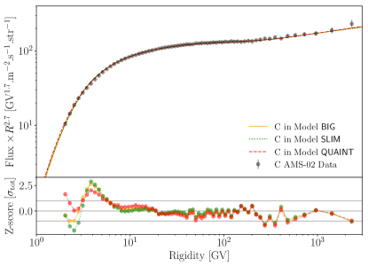
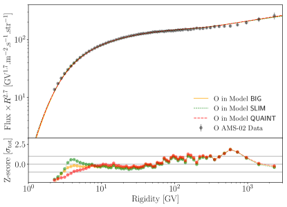
Figure 1: Combined best fits of C (top) and O (bottom) fluxes in the three benchmark models BIG, SLIM, and QUAINT defined by B/C fits (see Sect. IV). A panel below each plot reports the $Z$-score, corresponding to the residuals normalized by the total errors $\sigma_{\rm tot}$.

For the fits of the C and O fluxes, a simpler yet sufficient approximation is to assume uncorrelated total errors $\sigma_{\rm tot}$, i.e. statistical and systematic errors summed in quadrature: on the one hand, only statistical uncertainties dominate around the high-energy break position, so that this is a reasonable approximation. On the other hand, this fit only enters the B/C analysis via the treatment of the high-rigidity parameters as nuisance.

In Fig. 1 we report the fits of the source and high-rigidity break parameters to the C (top panel) and O (bottom panel) fluxes for our three benchmarks, the BIG, SLIM, and QUAINT models. It is clear even by visual inspection that the fits with a simple, common power-law index $\alpha$ are excellent: The fits fall within one $\sigma_{\rm tot}$ and never beyond two $\sigma_{\rm tot}$’s from all intermediate and high-rigidity points, showing that our consistency check is successful. Some minor discrepancy at low rigidity is noticeable, but not worrisome for our purposes. In fact, should one aim at describing C and O primary fluxes in detail down to low rigidities, a more accurate fitting procedure treating cross-section parameters as nuisance and accounting for bin-to-bin correlations of the systematic errors (as done for B/C) would certainly reduce these minor disagreements. This is beyond our goals here, but will be of interest for future more global analyses.

IV Results

In this section, we illustrate our results for the (low- and intermediate-rigidity) propagation parameters and discuss their implications. Initialization files used for the analysis, along with the resulting best-fit values and covariance matrix of best-fit parameters will be provided with the forthcoming new release usine v3.5.

IV.1 Best-fit values and $1\sigma$ uncertainties

The best-fit values and errors on the three model parameters (BIG, SLIM, and QUAINT) are reported in Tab. 2. In the first block, we report the diffusion parameters $\delta$ and $K_{10}$ common to all models, which control the intermediate-rigidity regime. We then report the low-rigidity parameters, which are different (both in nature and number) between QUAINT, on one side, and, BIG and SLIM, on the other. The high-rigidity break parameters, fixed following the nuisance procedure, are reported at the bottom of the Table. The range over which we scan for them will be discussed in App. A, since their determination is affected by the inclusion of external data (in our case, C and O absolute fluxes).

In all these fits, nuisance parameters vary within reasonable pre-assigned intervals. The solar modulation parameter $\phi_{\rm F}$ attains a value of 731, 734 and 725 MV in the best-fit model BIG, SLIM, and QUAINT, respectively. Concerning the nuisance of the spallation cross section $\rm{}^{12}C+H\rightarrow{}^{11}B$, its best normalization is found to be 12%, 13% and 11% above the reference GP17 value in the best-fit model BIG, SLIM, and QUAINT, respectively. The preferred slope encoding the low energy shape is of 0.12, 0 and 0.16, for the same models. The induced spectral distorsions in BIG and QUAINT  correspond to a slight decrease of the cross section at low energy.

Parameters	BIG	SLIM	QUAINT
$\chi^{2}/{\rm dof}$	$61.7/61\!=\!1.01$	$61.8/63\!=\!0.98$	$62.1/62\!=\!1.00$
Intermediate-rigidity parameters
$K_{10}$ [kpc2 Myr-1]	$0.30_{-0.04}^{+0.03}$	$0.28_{-0.02}^{+0.02}$	$0.33^{+0.03}_{-0.06}$
$\delta$	$0.48_{-0.03}^{+0.04}$	$0.51_{-0.02}^{+0.02}$	$0.45_{-0.02}^{+0.05}$
Low-rigidity parameters
$V_{\rm c}$ [km s-1]	$0^{+7.4}$	N/A	$0.0^{+8}$
$V_{\rm A}$ [km s-1]	$67^{+24}_{-67}$	N/A	$101_{-15}^{+14}$
$\eta$	1 (fixed)	1 (fixed)	$-0.09_{-0.57}^{+0.35}$
$\delta_{\rm l}$	$-0.69^{+0.61}_{-1.26}$	$-0.87^{+0.33}_{-0.31}$	N/A
$R_{\rm l}$ [GV]	$3.4_{-0.9}^{+1.1}$	$4.4_{-0.2}^{+0.2}$	N/A
High-rigidity break parameters
(nuisance parameters)
$\Delta_{\rm h}$	$0.18$	$0.19$	$0.17$
$R_{\rm h}$ [GV]	$247$	$237$	$270$
$s_{\rm h}$	$0.04$	$0.04$	$0.04$

Table 2: Best-fit parameter values and uncertainties for the three benchmark models BIG, SLIM, and QUAINT and corresponding $\chi^{2}/{\rm dof}$. The high-rigidity break parameters are nuisance parameters in the fit (see also text and App. A), and their preferred post-fit values are also quoted for the sake of completeness. Errors in italic are those that reach the allowed boundaries.

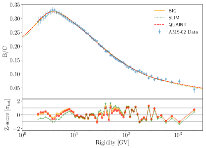
Figure 2: Best fit B/C curve for models BIG, SLIM, and QUAINT. Results for the best fit parameter values are given in Tab. 2. The bottom panel shows the $Z$-score.

Our best-fit curves are reported in Fig. 2 for the three models. Note that all models lead to analogous curves and fit quality, only differing in the fine features of the spectral shape at low rigidity. The inset displays the $Z$-score, i.e. the residuals normalized to the total errors $\sigma_{\rm tot}$. Note that this has only a qualitative purpose, since technically the $\chi^{2}$ is computed accounting for correlations in the systematics of B/C data, a major novelty of this analysis. The similar fit quality of the BIG and SLIM models indicates that the additional free parameters present in the former are actually unnecessary to describe the data: If the fit allows for a low-rigidity break, there is but a minor and currently unnecessary role played by $V_{\rm c}$ and $V_{\rm A}$. We note a tiny and statistically insignificant preference for model SLIM (and a fortiori BIG) with respect to QUAINT, which is only worth noticing since QUAINT has one free parameter more than in SLIM. In fact, we stress that if we had fixed $\eta=1$ in the QUAINT model, its fit quality would have degraded, and it would have been rejected at $>2\,\sigma$ with respect to the BIG and SLIM models. Finally, we note that, compare to SLIM, the benchmark BIG and QUAINT have respectively a weaker and no break at low rigidity, althought the latter is partly mimicked by the spectral distorsions of the cross section in nuisance. This tends to provide additional support to the possible presence of a low-rigidity break in the diffusion coefficient.

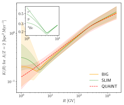
Figure 3: The diffusion coefficients corresponding to the three fits reported in Tab. 2 and Fig. 2, with their associated 1$\sigma$ uncertainty bands. We stress that the scaling at low rigidity depends on where the onset of the non-relativistic regime is located; here the curves are traced for a mass/charge ratio $A/Z=2$. For illustration, the inset shows the low rigidity regime for various species with different mass/charge values in the SLIM model.

Also, it is important to notice that the parameters common to the three models are found with values compatible within $\sim 1\sigma$. This suggests that the diffusive properties at intermediate rigidities are constrained rather robustly by the data (see Fig. 3 for an illustration of this), independently of the specific scenario within which the low-rigidity behavior is interpreted and fitted. This conclusion is rather encouraging when one considers interpretations of the high-rigidity spectral break.

The QUAINT model comes out with a few apparently surprising features: at face value, the best fit for $V_{\rm A}$ is rather large, perhaps even more so in the light of the value found for $V_{\rm c}$ which is compatible with zero. A too large value for $V_{\rm A}$ would lead to the surprising conclusion that the power in diffusive reacceleration is comparable to the total CR luminosity. This would for instance imply that the bulk of CRs energy rather originates from ISM turbulence than from shocks in SNRs, as customarily assumed (see e.g.(Drury and Strong, 2017)). This apparent conundrum is alleviated once accounting for the effective nature of our parameterization of the reacceleration term, which for technical reasons is artificially pinched to the thin disk, rather than being present in the whole propagation halo. The actual power in the turbulence in the whole Galaxy is thus reduced by the ratio $h/z_{\rm A}\simeq{\cal O}(h/L)$ (see Sect. II.1.3), hence resulting roughly consistent with expectations, and also more in line with the allowed range for $V_{\rm c}$. Another perhaps surprising outcome is the value of $\eta$, whose best fit is negative, and anyway rather away from typically considered values $\simeq 1$. This conclusion is also qualitatively valid in models BIG and SLIM: there is a slight preference for the diffusion coefficient below about 4.5 GV to increase with lower rigidity. Note that, within the allowed range for $\delta_{l}$, extrapolation in the non-relativistic regime could lead to nonphysical results, as soon as $\delta_{l}+1=\delta-\Delta_{\rm l}+1<0$. Be that as it may, neither this caveat nor the previous one for $\eta$ in the QUAINT model should be overstated, since they arise at best at the $1\sigma$ level. All model fits are consistent with a perhaps more physically acceptable flat behavior, or a rigidity-independent diffusion coefficient at low-$R$. Furthermore, it is worth noting how the BIG model is closer to the relatively unproblematic regime $\delta_{\rm l}>-1$ than the SLIM one. The introduction of some reacceleration and convection (both physically expected) tends to yield more reasonable values for the low-rigidity slope.

IV.2 Possible interpretation and microphysics

In any case, the most obvious interpretation of these results is that there are less and less waves onto which CRs can scatter at low rigidity. One possible reason is that turbulence dissipation effects lead to a parallel diffusion coefficient which decreases with increasing rigidity, with turning point at $\sim 3\;$GV for plausible choices for the parameters Shalchi and Büsching (2010). Another possibility arises in models where the CRs scatter onto self-generated turbulence below some rigidity (see e.g. (Blasi et al., 2012)). The energy density (and the pressure) carried by CRs peaks at the few GV scale; above this rigidity, the induced diffusion coefficient increases with rigidity as customarily assumed, because of the relatively steep CR power-law spectrum. Below this rigidity, however, the lower the rigidity (or Larmor radius), the smaller the turbulence with respect to extrapolations, simply because there are less and less CRs that can generate it by streaming instability due to their spectral inflection. The order of magnitude of the break in the low-energy CR spectrum seems to be in the right ballpark, but these qualitative arguments deserve a more detailed investigation, which we postpone to future work.

IV.3 Robustness of low-, intermediate-, and high-rigidity parameters

A very encouraging finding is that, within uncertainties, the diffusive properties at intermediate rigidities do not depend on the specific scenario considered at low-rigidity. The value found for $\delta$ appears closer to a Kraichnan turbulence spectrum ($\delta\simeq 0.5$) than to a Kolmogorov one ($\delta\simeq 1/3$), although this conclusion should not be overstated since the model involves an effective isotropic diffusion coefficient. An indirect implication of this robustness is to increase the credibility in any deviation found at high rigidity, of course.

Concerning the low-rigidity regime, however, there are several important caveats, which suggest some prudence to avoid over-interpreting the values found. First of all, while there is a clear indication for a different regime of propagation at low rigidity, the “hardest” parameters to interpret ($\eta$ and $\delta_{\rm l}$) are actually heavily influenced by the one or two lowest-rigidity points. This is illustrated in more detail in App. B, where one can compare the behavior of $R_{\rm l}$ vs. $R_{\rm min}$ with respect to $\delta_{\rm l}$ vs. $R_{\rm min}$, $R_{\rm min}$ being the rigidity above which the fit is performed. There is simply not enough of a baseline at low rigidity in the AMS-02 data to unambiguously measure the slope in this range. Another point to keep in mind is that the low-rigidity range is quite influenced by the uncertainties in the nuclear cross sections and the treatment of solar modulation. Indeed, including the nuisance parameters for the production cross section increases the $1\sigma$ uncertainties on $\eta$ (QUAINT) by 50%, and on $R_{l}$ and $\delta_{l}$ (BIG) by 90%. In our fits, including solar modulation is a second order effect, since it increases the low-energy parameters uncertainties by order 5%.

The only model-independent conclusion that we can safely make on the low-rigidity range is that multiple models can account for the observations, with rather different physical interpretations possible. So, statements such as “the reacceleration/convection velocity determined from the B/C data is …” should be taken with a grain of salt, since they appear very model dependent, if compared, for instance, with the determination of $\delta$. The fitted values should only be used as references in the same model used to fit them, and extrapolations at lower rigidities (below the range covered by the data) are not guaranteed to be physical.

V Summary, conclusions, and perspectives

This article has set the stage for the propagation scenarios that we want to test, challenge and refine with further AMS-02 data, defining benchmark models and ranges of parameters. We have validated the first step of this program with a statistically more sound analysis of the AMS-02 B/C data, going beyond state-of-the-art in the modern literature, and checking different theoretical frameworks differing in the treatment of transport at low rigidities with a major (model QUAINT) or a negligible (model SLIM) role played by reacceleration. Both models are limiting cases of a more general model (BIG). We have made sure that issues like numerical stability, the effects of cross sections uncertainties, the bin-to-bin correlation of systematic errors are handled sufficiently well not to bias significantly the conclusions.

For the time being, either model can describe with comparable performances the low-rigidity regime, with a statistically insignificant preference for model SLIM. The parameters describing intermediate rigidities are consistently determined in either case. At low rigidity, degeneracies with nuisance parameters impact both the best fit and uncertainties, in particular the ones controlling the energy shape of cross sections and solar modulation. This means that qualitatively different models offer almost equally good description of the data, so that inferring the physics of the propagation at low rigidity is challenging, and we must content ourselves with one or another “effective” description. This lesson on the shaky discrimination power among models with mild differences at low rigidities is likely to apply more generally, even to alternative models not tested here, because it partially relies on the effect of the nuisance parameters. Obviously, any discrimination between the two sets of models must be based on complementary data or arguments, such as the (astro)physical plausibility of the parameters found, an issue which we also briefly discussed. However, finding a break in the diffusion coefficient at low rigidity should not come so much as a surprise, since this feature, possibly related to some damping in the turbulence spectrum and the subsequent increase of the CR mean free path, is expected from theoretical grounds Yan and Lazarian (2004); Ptuskin et al. (2006); Shalchi and Büsching (2010); Evoli and Yan (2014). In this respect, a careful study of low energy data complimentary to AMS-02 ones (e.g. from ACE-CRIS Lave et al. (2013) and Voyager I Cummings et al. (2016); Webber et al. (2017)), together with a more realistic account of the systematic error correlations (based on further information provided by the experimental collaborations), could certainly help in drawing more robust conclusions on the properties and the nature of this break.

Besides extracting reference propagation parameters and uncertainty ranges from B/C data, which are intended for references for further studies, we have also performed a first test of the consistency of the obtained results with simple CR source spectra (power laws). We also confirmed and strengthened our conclusions in Génolini et al. (2017), that the high-rigidity data can be consistently interpreted as a consequence of a break in the diffusive coefficient, in agreement with AMS-02 high-energy primaries spectra. Indeed, we show that this preference does persist in a generalized analysis extending to the whole rigidity range, and for alternative propagation setups, notably with/without reacceleration.

Following this study, the most pressing issue is of course to test the reference models provided here against other secondary data (e.g., Li, Be, pbar, positrons). In particular, our forthcoming publication will focus on the antiproton channel Boudaud et al. (2019). There has been a recent interest in the possibility that these data hide a signal of dark matter annihilation, see e.g. Cuoco et al. (2019); Cholis et al. (2019), and it is interesting and important to re-examine those claims within our analysis framework. Finally, it is also known that putative dark matter signals are sensitive to the diffusive halo size, hence an important and motivated follow-up project analysis will involve other secondaries, including isotopes such as the radioactive species (e.g. ¹⁰Be). To that purpose, we provide the reader in App. C (1D models) and in App. D (2D models) with the scaling relations that allow to extrapolate our benchmark models (derived assuming $L=10$ kpc) to a range of $L$ between 4 and 18 kpc.

Note added: As we were completing this study, we became aware of Vittino et al. (2019), where the authors find support for the presence of multiple breaks in the diffusion coefficient, based on CR electron and positron data. This result is complementary to (and consistent with) ours, while interestingly based on independent datasets concerning other CR species.

Appendix A On the high-rigidity break from C, O and the fitting procedure

The fitting procedure described in Sect. III makes use of the C and O fluxes:

1. As a sanity check for the actual diffusion parameters inferred (see Fig. 1).

2. To determine $\alpha$, the common spectral index for all nuclei, although its value is irrelevant for the B/C calculation (and for the transport parameter determination).

3. Above all, for cornering a plausible window for the nuisance of the the high-energy break parameters.

Below, we provide some consistency checks as well as some comments on these ancillary results.

A.1 Consistency check

In Tab. 3, we report the results of the reference fits of C, O fluxes corresponding to the B/C model fits discussed in Sect. II.

Parameters	BIG	SLIM	QUAINT
$\chi^{2}/{\rm dof}$	$75.7/129=0.59$	$73.2/129=0.57$	$80.3/129=0.62$
$\alpha$	2.35	2.33	2.36
$\Delta_{\rm h}$	$0.18_{-0.05}^{+0.13}$	$0.18^{+0.11}_{-0.04}$	$0.18_{-0.01}^{+0.18}$
$R_{\rm h}$ [GV]	$244_{-52}^{+198}$	$236_{-51}^{+152}$	$282_{-89}^{\textit{+349}}$
$s_{\rm h}$	$0.04_{\it-0.04}^{+0.11}$	$0.03_{\textit{-0.03}}^{+0.09}$	${0.04}^{+0.15}_{\textit{-0.04}}$

Table 3: The $\chi^{2}/{\rm dof}$, the best-fit value for $\alpha$ as well as error range (used as nuisance parameters and ranges in the B/C analysis) for the high-rigidity parameters, coming from the combined fit to absolute C, O fluxes in the iterative procedure described in Sect. III. Values in italics means that the fit reached the border of the interval.

All propagation models inferred from B/C appear to provide excellent fits to the C, O fluxes as well. The $\chi^{2}$ cannot be used at face value as a quantitative estimator of the quality of the fit, since total errors have been used in the C, O fits: Hence, we likely underestimate the contribution to the $\chi^{2}$, notably those of the intermediate- and low-rigidity data mostly influenced by systematic errors and their correlations (see also the companion paper (Derome et al., 2019)). Nonetheless, a relative preference seems to emerge for the BIG and SLIM models, compared to the QUAINT model, which is interesting as the same trend is also present from the more rigorous B/C analysis.

Concerning $\alpha$, the values found are intriguingly similar to the ones found in the fit of the He flux, which is performed in (Boudaud et al., 2019), another reassuring consistency test of our procedure. We are thus consistent with the current universality of the spectra of nuclei (while the proton flux seems to be somewhat steeper). This is an interesting observable to keep an eye on in the future, of course. Note that the fit yields a nominal error on the parameter $\alpha$ at the sub-percent level, since $\delta$ is kept fixed in the iteration. Realistic uncertainties on $\alpha$ are however comparable to the ones of $\delta$ reported in Tab. 2.

In all cases, the indication for a high-rigidity break $\Delta_{\rm h}$ is rather significant ($\gtrsim 4\,\sigma$), again consistently with AMS-02 results, but here referring to the underlying diffusive coefficient (i.e. a break in the model space, not in the flux spectral index). Also, the values found are consistent within the errors with those found from $p$, He analyses (e.g. (Génolini et al., 2017)), although a bit higher, i.e. indicating a slightly more pronounced break. It will be interesting to follow-up on this in the light of further analyses of both light and intermediate/heavy nuclei, to see if the situation will relax towards a more common value or point to some discrepant hardening.

Let us briefly develop further on the significance of the high-rigidity break in the light of B/C data only.

Parameters	BIG	SLIM	QUAINT
$\delta$	$0.55_{-0.04}^{+0.20}$	$0.55^{+0.09}_{-0.03}$	${\it 0.9}_{-0.23}$
$K_{10}$ [kpc2/Myr]	$0.26_{-0.2}^{+0.05}$	$0.26_{-0.01}^{+0.07}$	$0.10^{+0.07}_{-0.01}$
$V_{\rm A}$ [km/s]	$0^{+64}$	NA	$71_{-7}^{+20}$
$V_{\rm c}$ [km/s]	$0^{+16}$	NA	$19_{-5}^{+3}$
$\eta_{t}$	1 (fixed)	1 (fixed)	$-0.30_{-0.75}^{+0.54}$
$\delta_{\rm l}$	$-0.84^{+0.32}_{-0.36}$	$-0.87^{+0.35}_{-0.33}$	NA
$R_{\rm l}$ [GV]	$4.4_{-2.1}^{+0.46}$	$4.4^{+0.2}_{-0.2}$	NA
$\Delta_{\rm h}$	$0.27_{-0.12}^{+0.22}$	$0.27_{{\it-0.12}}^{+0.21}$	$0.56_{-0.24}^{+0.09}$
$R_{\rm h}$ [GV]	$158_{{\it-58}}^{+235}$	$159^{+240}_{{\it-59}}$	${\it 100}^{+96}$
$s_{\rm h}$	$0.10_{{\it-0.10}}^{{\it+0.20}}$	$0.11_{-0.1}^{{\it+0.19}}$	$0.26_{{\it-0.26}}^{\it+0.04}$
$\chi^{2}/{\rm dof}$	$58.6/58=1.01$	$58.7/60=0.98$	$59.7/59=1.01$

Table 4: Best fit parameters for models BIG, SLIM, and QUAINT, if fitting the high-energy break of the diffusion coefficient as well on the B/C data only. Values in italics means that the fit reached the border of the interval.

If we were to use solely B/C data to fit also the high-rigidity parameters (i.e. without relying on the C, O flux data), we would obtain the results listed in Table IV. The low and intermediate rigidity propagation parameters are consistent with our reference one (see Tab. 2), with larger error bars, as expected since we now are determining more parameters from a more restricted set of data. Similar considerations apply to high-rigidity parameters, compare with Tab. 3. The largest departures are seen in the QUAINT model, where one suffers from a partial degeneracy of the (large) $V_{\rm A}$ parameter with the others, including $\delta$. Also, in this case parameters tend to drift towards the borders of the “plausible” interval fixed beforehand, which puts into question how physically meaningful this model results really are. Still, in all cases there is an evidence for a high-rigidity break (at $\gtrsim 2\,\sigma$ level, naively speaking) from the B/C alone, which a posteriori is a justification for our choice of the parameterization of the diffusion coefficient, Eq. (3).

A.2 Break vs no-break

In Tab. V we report the best fit propagation parameters without high-rigidity break in the diffusion coefficient. Note how the values of $\delta$ would be biased (at the $1\div 2\,\sigma$ level), resulting in a harder diffusion coefficient. In the same spirit as Génolini et al. (2017), we compute the $\Delta\chi^{2}$ with respect to our results in Tab. 2 (break parameters fit to C and O fluxes). In the QUAINT model, as intuitively expected, the presence of a large $V_{\rm A}$ can partially mimic the break, but not completely, and the “no break” case is still disfavored (at $\sim 2\,\sigma$ level). For the BIG and SLIM models, which are refinements of the purely diffusive intermediate/high-rigidity model considered in Génolini et al. (2017), we find $\Delta\chi^{2}>10$, confirming (and thus reinforcing the robustness of) the results presented in Génolini et al. (2017).

Parameters	BIG	SLIM	QUAINT
$\delta$	$0.48^{+0.02}_{-0.02}$	$0.48^{+0.02}_{-0.02}$	$0.42^{+0.03}_{-0.02}$
$K_{10}$ [kpc2/Myr]	$0.29^{+0.02}_{-0.02}$	$0.29^{+0.02}_{-0.02}$	$0.36^{+0.02}_{-0.04}$
$V_{\rm A}$ [km/s]	$0^{+115}$	NA	$113^{+7}_{-15}$
$V_{\rm c}$ [km/s]	$0^{+12}$	NA	$0^{+4.1}$
$\eta_{t}$	1 (fixed)	1 (fixed)	$0.6^{+0.3}_{-0.5}$
$\delta_{\rm l}$	$-0.88_{-0.30}^{+0.31}$	$-0.88_{-0.30}^{+0.32}$	NA
$R_{\rm l}$ [GV]	$4.4^{+0.23}_{-2.4}$	$4.4^{+0.24}_{-0.21}$	NA
$\chi^{2}/{\rm dof}$	$72.8/61=1.19$	$72.8/63=1.16$	$67.1/62=1.08$
$\Delta\chi^{2}$	11.1	11.0	5.0

Table 5: Best fit parameters for models BIG, SLIM, and QUAINT, with no high-rigidity break in the diffusion coefficient.

Appendix B Fit parameters dependence upon low-rigidity cutoff

In Fig. 4, we present the evolution of the best-fit parameters as a function of a low-rigidity cut $R_{\rm min}$ above which the fit is performed, for the three models considered. We note that the value of the parameters $\delta$ and $K_{10}$ remains essentially unchanged whatever $R_{\rm min}$. In contrast, $\delta_{\rm l}$, $R_{\rm l}$ (for BIG and SLIM), $V_{a}$, and $\eta$ (for QUAINT) depend crucially on the first data points, notably those below $\sim$4 GV. This explains their denomination of low-rigidity parameters. For the SLIM model, note how the error on $\delta_{\rm l}$ crucially depends on the first couple of AMS-02 points, and the evidence for a change of slope (a determination of $R_{\rm l}$) is stronger than the actual value of the slope at low rigidity. Finally, it is worth commenting on $V_{\rm A}$: this parameter is (anti)correlating with low-energy ones (in particular $\eta$ for QUAINT) and, to a minor extent, also with $\delta$. This is not very surprising since large values of $V_{\rm A}$ imply “cross-talk” among energy bins.

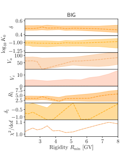
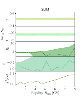
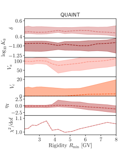
Figure 4: Evolution of the best fit parameter values and uncertainties as a function of the minimal rigidity $R_{\rm min}$ above which the fit is performed, for the three benchmark models BIG, SLIM and QUAINT. Note that in this figure only we use $K_{0}$ (normalization of $K$ at $R=1\,$GV) instead of $K_{10}$.

Appendix C Scaling of propagation parameters with $L$ in 1D model

The benchmark parameters for BIG, SLIM, and QUAINT where derived assuming the Galactic magnetic halo shapes as a 1D-slab of half-thickness $L=10$ kpc. By fitting the B/C ratio in these models, it is well known that the normalization of the diffusion coefficient $K_{10}$ and the halo thickness $L$ are degenerated so that the ratio $K_{10}/L$ is constant. We have checked that this was still the case given the higher sensitivity of AMS-02 data, and found the following scaling relations for values of $L$ within [4,18] kpc:

$$\text{{\sf BIG}: }\quad\frac{K_{10}}{L}=0.030^{+0.003}_{-0.004}\;\rm kpc/Myr\;.$$ (7a)

$$\text{{\sf SLIM}: }\quad\frac{K_{10}}{L}=0.028^{+0.002}_{-0.002}\;\rm kpc/Myr\;,$$ (7b)

$$\text{{\sf QUAINT}: }\quad\frac{K_{10}}{L}=0.033^{+0.003}_{-0.006}\;\rm kpc/Myr\;.$$ (7c)

Appendix D Dictionary to use 1D propagation parameters in 2D models.

A 1D-slab geometry for the magnetic halo does not allow one to account for CRs escaping radially from the Galaxy (see, e.g. refs Taillet and Maurin (2003); Maurin and Taillet (2003)). This choice could be thought as an over-simplification. A more realistic 2D geometry commonly used is to consider the Galactic halo as a cylindrical box of radius 20 kpc and half-thickness $L=10$ kpc, where CR sources lie uniformly in the disk and the Earth is set at 8.5 kpc from its center (for an illustration see e.g. Fig.10 of Genolini et al. (2015)). However, using this geometry we have found that variations of the best fit values (Tab. 2) for all parameters, except $K_{10}$, are within their respective uncertainties. In fact, in this 2D (uniform disk) case, a degeneracy between $K_{10}$ and $L$ is still present, but is no longer described by the relation Eq. (7); the escape from the radial boundaries increases with increasing $L$. Starting from Tab. 2, for each benchmark, we summarize below our empirical prescription to go from 1D to 2D, only for the parameters which drift with $L$. Note that the preferred value for $V_{\rm A}$ in the BIG model is now zero, although the uncertainty on this parameter is quite large.

$$\text{{\sf BIG}: }\,\frac{K^{\rm 2D}_{10}}{\tanh{(L^{1.1}/10.1)}}=0.25^{+0.04}_{-0.02}\,{\rm kpc^{2}/Myr},\quad\delta^{2D}\times\tanh{(L^{0.4}/0.77)}=0.50^{+0.02}_{-0.04}\quad\text{and}\quad\begin{cases}V_{\rm A}=0^{+80}\,{\rm km.s^{-1}}\\ R_{\rm l}=4.4_{-0.2}^{+0.2}\,{\rm GV}\\ \delta_{\rm l}=-0.83_{-0.3}^{+0.3}\end{cases}\,,$$

$$\text{{\sf SLIM}: }\,\frac{K^{\rm 2D}_{10}}{\tanh{(L^{1.1}/10.1)}}=0.25^{+0.02}_{-0.02}\,{\rm kpc^{2}/Myr}\quad\text{and}\quad\delta^{2D}\times\tanh{(L^{0.4}/0.77)}=0.50^{+0.02}_{-0.02}\,,$$

$$\text{{\sf QUAINT}: }\,\frac{K^{\rm 2D}_{10}}{\tanh{(L^{1.1}/10.1)}}=0.30^{+0.02}_{-0.07}\,{\rm kpc^{2}/Myr}\quad\text{and}\quad\delta^{2D}\times\tanh{(L^{0.4}/0.77)}=0.44^{+0.06}_{-0.02}\,.$$

References

- Ahn et al. (2009) H. S. Ahn et al. (CREAM Collaboration), ApJ 707, 593 (2009), arXiv:0911.1889 [astro-ph.HE] .
- Panov et al. (2009) A. D. Panov et al. (ATIC-2 Collaboration), Bulletin of the Russian Academy of Sciences, Physics 73, 564 (2009), arXiv:1101.3246 [astro-ph.HE] .
- Adriani et al. (2014) O. Adriani et al. (PAMELA Collaboration), Phys. Rep. 544, 323 (2014).
- Ting (2013) S. Ting, Nuclear Physics B Proceedings Supplements 243, 12 (2013).
- Adriani et al. (2017) O. Adriani et al. (CALET Collaboration), Phys. Rev. Lett. 119, 181101 (2017), arXiv:1712.01711 [astro-ph.HE] .
- Ambrosi et al. (2017) G. Ambrosi et al. (DAMPE Collaboration), Nature 552, 63 (2017), arXiv:1711.10981 [astro-ph.HE] .
- Mertsch (2011) P. Mertsch, J. Cosmology Astropart. Phys. 2, 031 (2011), arXiv:1012.0805 [astro-ph.HE] .
- Genolini et al. (2017) Y. Genolini, P. Salati, P. D. Serpico, and R. Taillet, A&A 600, A68 (2017), arXiv:1610.02010 [astro-ph.HE] .
- Aguilar et al. (2016) M. Aguilar et al. (AMS-02 Collaboration), Phys. Rev. Lett. 117, 231102 (2016).
- Coste et al. (2012) B. Coste, L. Derome, D. Maurin, and A. Putze, A&A 539, A88 (2012), arXiv:1108.4349 [astro-ph.GA] .
- Owens (1976) A. J. Owens, Ap&SS 44, 35 (1976).
- Ginzburg et al. (1980) V. L. Ginzburg, I. M. Khazan, and V. S. Ptuskin, Ap&SS 68, 295 (1980).
- Protheroe et al. (1981) R. J. Protheroe, J. F. Ormes, and G. M. Comstock, ApJ 247, 362 (1981).
- Strong and Moskalenko (1998) A. W. Strong and I. V. Moskalenko, ApJ 509, 212 (1998), astro-ph/9807150 .
- Maurin et al. (2001) D. Maurin, F. Donato, R. Taillet, and P. Salati, ApJ 555, 585 (2001), astro-ph/0101231 .
- Maurin et al. (2002a) D. Maurin, R. Taillet, and F. Donato, A&A 394, 1039 (2002a), astro-ph/0206286 .
- Putze et al. (2011) A. Putze, D. Maurin, and F. Donato, A&A 526, A101 (2011), arXiv:1011.0989 [astro-ph.GA] .
- Genolini et al. (2015) Y. Genolini, A. Putze, P. Salati, and P. D. Serpico, A&A 580, A9 (2015), arXiv:1504.03134 [astro-ph.HE] .
- Malkov and Drury (2001) M. A. Malkov and L. O. Drury, Reports on Progress in Physics 64, 429 (2001).
- Caprioli and Spitkovsky (2014) D. Caprioli and A. Spitkovsky, ApJ 783, 91 (2014), arXiv:1310.2943 [astro-ph.HE] .
- Amato (2014) E. Amato, International Journal of Modern Physics D 23, 1430013 (2014), arXiv:1406.7714 [astro-ph.HE] .
- Marcowith et al. (2016) A. Marcowith, A. Bret, A. Bykov, M. E. Dieckman, L. O’C Drury, B. Lembège, M. Lemoine, G. Morlino, G. Murphy, G. Pelletier, I. Plotnikov, B. Reville, M. Riquelme, L. Sironi, and A. Stockem Novo, Reports on Progress in Physics 79, 046901 (2016), arXiv:1604.00318 [astro-ph.HE] .
- Génolini et al. (2017) Y. Génolini, P. D. Serpico, M. Boudaud, S. Caroff, V. Poulin, L. Derome, J. Lavalle, D. Maurin, V. Poireau, S. Rosier, P. Salati, and M. Vecchi, Phys. Rev. Lett. 119, 241101 (2017), arXiv:1706.09812 [astro-ph.HE] .
- Aguilar et al. (2015) M. Aguilar et al. (AMS-02 Collaboration), Phys. Rev. Lett. 114, 171103 (2015).
- Serpico (2015) P. D. Serpico, in 34th International Cosmic Ray Conference (ICRC2015), International Cosmic Ray Conference, Vol. 34, edited by A. S. Borisov, V. G. Denisova, Z. M. Guseva, E. A. Kanevskaya, M. G. Kogan, A. E. Morozov, V. S. Puchkov, S. E. Pyatovsky, G. P. Shoziyoev, M. D. Smirnova, A. V. Vargasov, V. I. Galkin, S. I. Nazarov, and R. A. Mukhamedshin (2015) p. 9, arXiv:1509.04233 [astro-ph.HE] .
- Serpico (2018) P. D. Serpico, Journal of Astrophysics and Astronomy 39, 41 (2018).
- Ahn et al. (2010) H. S. Ahn et al. (CREAM Collaboration), ApJ 714, L89 (2010), arXiv:1004.1123 [astro-ph.HE] .
- Adriani et al. (2011) O. Adriani et al. (PAMELA Collaboration), Science 332, 69 (2011), arXiv:1103.4055 [astro-ph.HE] .
- Aguilar et al. (2015) M. Aguilar et al. (AMS-02 Collaboration), Phys. Rev. Lett. 115, 211101 (2015).
- Aguilar et al. (2017) M. Aguilar et al. (AMS-02 Collaboration), Phys. Rev. Lett. 119, 251101 (2017).
- Reinert and Winkler (2018) A. Reinert and M. W. Winkler, J. Cosmology Astropart. Phys. 1, 055 (2018), arXiv:1712.00002 [astro-ph.HE] .
- Xue and Niu (2019) H.-F. Xue and J.-S. Niu, arXiv e-prints (2019), arXiv:1902.09343 [astro-ph.HE] .
- Aguilar et al. (2018) M. Aguilar et al. (AMS-02 Collaboration), Phys. Rev. Lett. 120, 021101 (2018).
- Génolini et al. (2018) Y. Génolini, D. Maurin, I. V. Moskalenko, and M. Unger, Phys. Rev. C 98, 034611 (2018), arXiv:1803.04686 [astro-ph.HE] .
- Derome et al. (2019) L. Derome, D. Maurin, P. Salati, M. Boudaud, Y. Génolini, and P. Kunzé, arXiv e-prints (2019), arXiv:1904.08210 [astro-ph.HE] .
- Maurin (2018) D. Maurin, ArXiv e-prints (2018), arXiv:1807.02968 [astro-ph.IM] .
- Evoli et al. (2008) C. Evoli, D. Gaggero, D. Grasso, and L. Maccione, J. Cosmology Astropart. Phys. 10, 018 (2008), arXiv:0807.4730 .
- Evoli et al. (2017) C. Evoli, D. Gaggero, A. Vittino, G. Di Bernardo, M. Di Mauro, A. Ligorini, P. Ullio, and D. Grasso, J. Cosmology Astropart. Phys. 2, 015 (2017), arXiv:1607.07886 [astro-ph.HE] .
- Kissmann (2014) R. Kissmann, Astroparticle Physics 55, 37 (2014), arXiv:1401.4035 [astro-ph.HE] .
- Kissmann et al. (2015) R. Kissmann, M. Werner, O. Reimer, and A. W. Strong, Astroparticle Physics 70, 39 (2015), arXiv:1504.08249 [astro-ph.HE] .
- Delahaye et al. (2009) T. Delahaye, R. Lineros, F. Donato, N. Fornengo, J. Lavalle, P. Salati, and R. Taillet, A&A 501, 821 (2009), arXiv:0809.5268 .
- Delahaye et al. (2010) T. Delahaye, J. Lavalle, R. Lineros, F. Donato, and N. Fornengo, A&A 524, A51 (2010), arXiv:1002.1910 [astro-ph.HE] .
- Boudaud et al. (2017a) M. Boudaud, E. F. Bueno, S. Caroff, Y. Genolini, V. Poulin, V. Poireau, A. Putze, S. Rosier, P. Salati, and M. Vecchi, A&A 605, A17 (2017a), arXiv:1612.03924 [astro-ph.HE] .
- Donato et al. (2001) F. Donato, D. Maurin, P. Salati, A. Barrau, G. Boudoul, and R. Taillet, ApJ 563, 172 (2001), astro-ph/0103150 .
- Giesen et al. (2015) G. Giesen, M. Boudaud, Y. Génolini, V. Poulin, M. Cirelli, P. Salati, and P. D. Serpico, J. Cosmology Astropart. Phys. 9, 023 (2015), arXiv:1504.04276 [astro-ph.HE] .
- Boudaud et al. (2019) M. Boudaud, D. Maurin, L. Derome, Y. Génolini, J. Lavalle, P. Salati, P. D. Serpico, and M. Vecchi, In preparation (2019).
- Delahaye et al. (2008) T. Delahaye, R. Lineros, F. Donato, N. Fornengo, and P. Salati, Phys. Rev. D 77, 063527 (2008), arXiv:0712.2312 .
- Boudaud et al. (2015a) M. Boudaud, M. Cirelli, G. Giesen, and P. Salati, J. Cosmology Astropart. Phys. 5, 013 (2015a), arXiv:1412.5696 [astro-ph.HE] .
- Boudaud et al. (2015b) M. Boudaud, S. Aupetit, S. Caroff, A. Putze, G. Belanger, Y. Genolini, C. Goy, V. Poireau, V. Poulin, S. Rosier, P. Salati, L. Tao, and M. Vecchi, A&A 575, A67 (2015b), arXiv:1410.3799 [astro-ph.HE] .
- Boudaud et al. (2017b) M. Boudaud, J. Lavalle, and P. Salati, Phys. Rev. Lett. 119, 021103 (2017b), arXiv:1612.07698 [astro-ph.HE] .
- Boudaud and Cirelli (2018) M. Boudaud and M. Cirelli, ArXiv e-prints (2018), arXiv:1807.03075 [astro-ph.HE] .
- Boudaud et al. (2018) M. Boudaud, T. Lacroix, M. Stref, and J. Lavalle, ArXiv e-prints (2018), arXiv:1810.01680 [astro-ph.HE] .
- Donato et al. (2004) F. Donato, N. Fornengo, D. Maurin, P. Salati, and R. Taillet, Phys. Rev. D 69, 063501 (2004), astro-ph/0306207 .
- Lavalle et al. (2014) J. Lavalle, D. Maurin, and A. Putze, Phys. Rev. D 90, 081301 (2014), arXiv:1407.2540 [astro-ph.HE] .
- Amato and Blasi (2018) E. Amato and P. Blasi, Advances in Space Research 62, 2731 (2018), arXiv:1704.05696 [astro-ph.HE] .
- Ginzburg and Syrovatskii (1964) V. L. Ginzburg and S. I. Syrovatskii, The Origin of Cosmic Rays (New York: Macmillan, 1964).
- Berezinskii et al. (1990) V. S. Berezinskii, S. V. Bulanov, V. A. Dogiel, and V. S. Ptuskin, Astrophysics of cosmic rays (North Holland, 1990).
- Schlickeiser (2002) R. Schlickeiser, Cosmic ray astrophysics / Reinhard Schlickeiser, Astronomy and Astrophysics Library; Physics and Astronomy Online Library. Berlin: Springer. ISBN 3-540-66465-3, 2002, XV + 519 pp. (Springer Berlin Heidelberg, 2002).
- Mannheim and Schlickeiser (1994) K. Mannheim and R. Schlickeiser, A&A 286, 983 (1994), astro-ph/9402042 .
- Putze et al. (2010) A. Putze, L. Derome, and D. Maurin, Astron.Astrophys. 516, A66 (2010), arXiv:1001.0551 [astro-ph.HE] .
- Gleeson and Axford (1968) L. J. Gleeson and W. I. Axford, ApJ 154, 1011 (1968).
- Fisk (1971) L. A. Fisk, J. Geophys. Res. 76, 221 (1971).
- Ghelfi et al. (2016) A. Ghelfi, F. Barao, L. Derome, and D. Maurin, A&A 591, A94 (2016), arXiv:1511.08650 [astro-ph.HE] .
- Bulanov and Dogel (1974) S. V. Bulanov and V. A. Dogel, Ap&SS 29, 305 (1974).
- Ptuskin (1974) V. S. Ptuskin, Ap&SS 28, 17 (1974).
- Jones (1979) F. C. Jones, ApJ 229, 747 (1979).
- Ptuskin and Soutoul (1990) V. S. Ptuskin and A. Soutoul, A&A 237, 445 (1990).
- Jones et al. (2001) F. C. Jones, A. Lukasiak, V. Ptuskin, and W. Webber, ApJ 547, 264 (2001), astro-ph/0007293 .
- Ferrière (2001) K. M. Ferrière, Reviews of Modern Physics 73, 1031 (2001), astro-ph/0106359 .
- Maurin et al. (2010) D. Maurin, A. Putze, and L. Derome, A&A 516, A67 (2010), arXiv:1001.0553 [astro-ph.HE] .
- Casse et al. (2002) F. Casse, M. Lemoine, and G. Pelletier, Phys. Rev. D 65, 023002 (2002), astro-ph/0109223 .
- Sun et al. (2008) X. Sun, W. Reich, A. Waelkens, and T. Enslin, A&A 477, 573 (2008), arXiv:0711.1572 .
- Jansson and Farrar (2012) R. Jansson and G. R. Farrar, ApJ 757, 14 (2012), arXiv:1204.3662 .
- DeMarco et al. (2007) D. DeMarco, P. Blasi, and T. Stanev, J. Cosmology Astropart. Phys. 6, 027 (2007), arXiv:0705.1972 .
- Evoli et al. (2012) C. Evoli, D. Gaggero, D. Grasso, and L. Maccione, Phys. Rev. Lett. 108, 211102 (2012), arXiv:1203.0570 [astro-ph.HE] .
- Tomassetti (2012) N. Tomassetti, ApJ 752, L13 (2012), arXiv:1204.4492 [astro-ph.HE] .
- Guo and Yuan (2018) Y.-Q. Guo and Q. Yuan, Phys. Rev. D 97, 063008 (2018), arXiv:1801.05904 [astro-ph.HE] .
- Seo and Ptuskin (1994) E. S. Seo and V. S. Ptuskin, ApJ 431, 705 (1994).
- Blasi et al. (2012) P. Blasi, E. Amato, and P. D. Serpico, Phys. Rev. Lett. 109, 061101 (2012), arXiv:1207.3706 [astro-ph.HE] .
- Aloisio and Blasi (2013) R. Aloisio and P. Blasi, J. Cosmology Astropart. Phys. 7, 001 (2013), arXiv:1306.2018 [astro-ph.HE] .
- Aloisio et al. (2015) R. Aloisio, P. Blasi, and P. D. Serpico, A&A 583, A95 (2015), arXiv:1507.00594 [astro-ph.HE] .
- Evoli et al. (2018) C. Evoli, P. Blasi, G. Morlino, and R. Aloisio, Phys. Rev. Lett. 121, 021102 (2018), arXiv:1806.04153 [astro-ph.HE] .
- Wentzel (1969) D. G. Wentzel, ApJ 156, 303 (1969).
- Holmes (1975) J. A. Holmes, MNRAS 170, 251 (1975).
- Skilling (1975) J. Skilling, MNRAS 172, 557 (1975).
- Cummings et al. (2016) A. C. Cummings, E. C. Stone, B. C. Heikkila, N. Lal, W. R. Webber, G. Jóhannesson, I. V. Moskalenko, E. Orlando, and T. A. Porter, ApJ 831, 18 (2016).
- Webber et al. (2017) W. R. Webber, N. Lal, E. C. Stone, A. C. Cummings, and B. Heikkila, ArXiv e-prints (2017), arXiv:1712.02818 [physics.space-ph] .
- Yan and Lazarian (2004) H. Yan and A. Lazarian, ApJ 614, 757 (2004), astro-ph/0408172 .
- Ptuskin et al. (2005) V. S. Ptuskin, I. V. Moskalenko, F. C. Jones, A. W. Strong, and S. G. Mashnik, Advances in Space Research 35, 162 (2005), astro-ph/0301420 .
- Ptuskin et al. (2006) V. S. Ptuskin, I. V. Moskalenko, F. C. Jones, A. W. Strong, and V. N. Zirakashvili, ApJ 642, 902 (2006), astro-ph/0510335 .
- Shalchi and Büsching (2010) A. Shalchi and I. Büsching, ApJ 725, 2110 (2010).
- Evoli and Yan (2014) C. Evoli and H. Yan, ApJ 782, 36 (2014), arXiv:1310.5732 [astro-ph.HE] .
- Xu and Lazarian (2016) S. Xu and A. Lazarian, ApJ 833, 215 (2016), arXiv:1608.05161 .
- Jokipii (1966) J. R. Jokipii, ApJ 146, 480 (1966).
- Shalchi (2009) A. Shalchi, Nonlinear Cosmic Ray Diffusion Theories, Astrophysics and Space Science Library, Vol. 362 (Springer-Verlag Berlin Heidelberg, 2009).
- Dunkel et al. (2007) J. Dunkel, P. Talkner, and P. Hanggi, Phys. Rev. D 75, 043001 (2007), cond-mat/0608023 .
- Aloisio et al. (2009) R. Aloisio, V. Berezinsky, and A. Gazizov, ApJ 693, 1275 (2009), arXiv:0805.1867 .
- Osborne and Ptuskin (1988) J. L. Osborne and V. S. Ptuskin, Soviet Astronomy Letters 14, 132 (1988).
- Maurin et al. (2002b) D. Maurin, R. Taillet, F. Donato, P. Salati, A. Barrau, and G. Boudoul, ArXiv Astrophysics e-prints (2002b), astro-ph/0212111 .
- Thornbury and Drury (2014) A. Thornbury and L. O. Drury, MNRAS 442, 3010 (2014), arXiv:1404.2104 [astro-ph.HE] .
- Drury and Strong (2017) L. O. . Drury and A. W. Strong, A&A 597, A117 (2017), arXiv:1608.04227 [astro-ph.HE] .
- Lavalle and Salati (2012) J. Lavalle and P. Salati, Comptes Rendus Physique 13, 740 (2012), arXiv:1205.1004 [astro-ph.HE] .
- James and Roos (1975) F. James and M. Roos, Computer Physics Communications 10, 343 (1975).
- Lave et al. (2013) K. A. Lave, M. E. Wiedenbeck, W. R. Binns, E. R. Christian, A. C. Cummings, A. J. Davis, G. A. de Nolfo, M. H. Israel, R. A. Leske, R. A. Mewaldt, E. C. Stone, and T. T. von Rosenvinge, ApJ 770, 117 (2013).
- Cuoco et al. (2019) A. Cuoco, J. Heisig, L. Klamt, M. Korsmeier, and M. Krämer, arXiv e-prints (2019), arXiv:1903.01472 [astro-ph.HE] .
- Cholis et al. (2019) I. Cholis, T. Linden, and D. Hooper, arXiv e-prints (2019), arXiv:1903.02549 [astro-ph.HE] .
- Vittino et al. (2019) A. Vittino, P. Mertsch, H. Gast, and S. Schael, arXiv e-prints (2019), arXiv:1904.05899 [astro-ph.HE] .
- Taillet and Maurin (2003) R. Taillet and D. Maurin, Astron. Astrophys. 402, 971 (2003), arXiv:astro-ph/0212112 [astro-ph] .
- Maurin and Taillet (2003) D. Maurin and R. Taillet, Astron. Astrophys. 404, 949 (2003), arXiv:astro-ph/0212113 [astro-ph] .