The acceptance profile of invasion percolation at $p_{c}$ in two dimensions

Abstract

Invasion percolation is a stochastic growth model that follows a greedy algorithm. After assigning i.i.d. uniform random variables (weights) to all edges of $\mathbb{Z}^{d}$, the growth starts at the origin. At each step, we adjoin to the current cluster the edge of minimal weight from its boundary. In ’85, Chayes-Chayes-Newman studied the “acceptance profile” of the invasion: for a given $p\in[0,1]$, it is the ratio of the expected number of invaded edges until time $n$ with weight in $[p,p+\text{d}p]$ to the expected number of observed edges (those in the cluster or its boundary) with weight in the same interval. They showed that in all dimensions, the acceptance profile $a_{n}(p)$ converges to one for $p<p_{c}$ and to zero for $p>p_{c}$. In this paper, we consider $a_{n}(p)$ at the critical point $p=p_{c}$ in two dimensions and show that it is bounded away from zero and one as $n\to\infty$.

1 Introduction

1.1 The model

We begin with the definition of invasion percolation. It is a stochastic growth model introduced independently by two groups ([1] and [13]) and is a simple example of self-organized criticality. That is, although the model itself has no parameter, its structure on large scales resembles that of another critical model: critical Bernoulli percolation.

Let ${\mathbb{Z}}^{2}$ be the two-dimensional square lattice and $\mathcal{E}^{2}$ be the set of nearest-neighbor edges. For a subgraph $G=(V,E)$ of $({\mathbb{Z}}^{2},\mathcal{E}^{2})$, we define the outer (edge) boundary of $G$ as

$$\partial G:=\{e=\{x,y\}\in\mathcal{E}^{d}:e\notin E,\text{but}\;x\in V\;\text{or}\;y\in V\}.$$

Assign i.i.d uniform random $[0,1]$ variables $(\omega(e))$ to all bonds $e\in\mathcal{E}^{2}$. The invasion percolation cluster (IPC) $G$ can be defined as the limit of an increasing sequence of subgraphs $(G_{n})$ as follows. The graph $G_{0}$ has only the origin and no edges. Once $G_{i}=(V_{i},E_{i})$ is defined, we select the edge $e_{i+1}$ that minimizes $\omega(e)$ for $e\in\partial G_{i}$, take $E_{i+1}=E_{i}\cup\{e_{i+1}\}$ and let $G_{i+1}$ be the graph induced by the edge set $E_{i+1}$. The graph $G_{i}$ is called the invaded region at time $i$, and the graph $G=\cup_{i=0}^{\infty}G_{i}$ is called the invasion percolation cluster (IPC).

The first rigorous study of invasion percolation was done in ’85 by Chayes-Chayes-Newman [2], who took a dynamical perspective: their questions were related to the evolution of the graph $G_{n}$ as $n$ increases. In the ’90s and ’00s, results focused on a more static perspective: properties of the full invaded region. For example, the fractal dimension of $G$ was determined [19] along with finer properties of $G$ like relations to other critical models [10], analysis of the pond and outlet structure [3, 5], and scaling limits [6].

In this paper, we return to the earlier dynamical perspective and study the “acceptance profile” of the invasion, introduced in [18]. Roughly speaking, the acceptance profile $a_{n}(p)$ at value $p$ and time $n$ is the ratio

$$a_{n}(p)=\frac{\text{expected number of bonds invaded with weight in }[p,p+\text{d}p]}{\text{expected number of bonds observed with weight in }[p,p+\text{d}p]},$$

where both the numerator and denominator are computed until time $n$, and a bond is observed by time $n$ if it is either invaded by time $n$ or is on the boundary of the invasion at time $n$. In [2, Theorems 4.2, 4.3], it is shown that for general dimensions, if $p<\pi_{c}$ (a certain critical threshold for independent percolation), one has $a_{n}(p)\to 1$ as $n\to\infty$ and if $p>\bar{p}_{c}$ (another threshold value with $\bar{p}_{c}\geq\pi_{c}$), one has $a_{n}(p)\to 0$ as $n\to\infty.$ Since publication of that paper, it has been established that $\bar{p}_{c}=\pi_{c}=p_{c}$, where $p_{c}$ is the standard critical value for independent percolation. Since $p_{c}=1/2$ in dimension 2, we have

$$\lim_{n\to\infty}a_{n}(p)=\begin{cases}1&\quad\text{if }p<1/2\\ 0&\quad\text{if }p>1/2.\end{cases}$$

This result means that when $p<p_{c}$, all observed edges with weight near $p$ are invaded relatively quickly, whereas for $p>p_{c}$, observed edges with weight near $p$ are never invaded (for $n$ large).

The case $p=p_{c}$ was left open in [2], and it is this case we study here. It would be very interesting to establish the existence of $\lim_{n\to\infty}a_{n}(p_{c})$, which by the following main theorem, would be a number in $(0,1)$.

Theorem 1.1.

In two dimensions, where $p_{c}=1/2$,

$$0<\liminf_{n\rightarrow\infty}a_{n}(p_{c})\leq\limsup_{n\rightarrow\infty}a_{n}(p_{c})<1.$$

This theorem roughly states that when $n$ is large, at least $c\epsilon$ fraction of invaded edges have weight in $(p_{c},p_{c}+\epsilon]$, whereas at least $c\epsilon$ fraction of observed edges with weight in this interval are not yet invaded. To prove this result, we will need to study detailed properties of the invaded region at time $n$, which can be quite different than those of the full invaded region.

In the physics literature, the acceptance profile was considered earlier, in work of Wilkinson-Willemsen [18]. There, it was loosely defined as $a(r)$, the “number of random numbers in the interval $[r,r+\text{d}r]$ which were accepted into the cluster, expressed as a fraction of the number of random numbers in that range which became available.” It was noted in that paper that the acceptance profile appears to approach a step function with jump at $p_{c}$, and that for values of $p$ near $p_{c}$, “there is a transition region in which some numbers are accepted and some rejected.” (See [18, Fig. 2].) This observation, although for a different version of the acceptance profile (there is no expected value as in the acceptance profile of Chayes-Chayes-Newman that we work with), is consistent with our main theorem. The step function property of the profile has later been used to estimate numerical values of $p_{c}$ (see, for example, [17]).

In the next section, we give a rigorous definition of the acceptance profile along with the results of [2]. To do this, we will also introduce the standard Bernoulli percolation model.

1.2 Acceptance Profile

To define the acceptance profile, we use the notations of [2]. Let $I_{n}\in\mathcal{E}^{2}$ be the invaded bond at time $n\geq 1$ and let $x_{n}$ be the random weight of $I_{n}$ (the weight $\omega(I_{n})$). For any $y\in[0,1]$, define $X_{n}(y)$ as the indicator that $x_{n}\leq y$:

$$X_{n}(y)=\left\{\begin{array}[]{lr}1&\text{if}\;\;x_{n}\leq y\\ 0&\text{otherwise}.\end{array}\right.$$

Let $R_{n}$ be the random number of new bonds which must be checked after the invasion of $I_{n}$ (that is, $R_{0}=4$, $R_{1}=3$, and $R_{n}$ is the number of boundary edges of $G_{n}$ that were not boundary edges of $G_{n-1}$) and define $L_{n}:=\displaystyle\sum_{j=0}^{n}R_{j}$ to be the total number of checked bonds until the invasion of $I_{n}$. Clearly, $n\leq L_{n}\leq 4n$. Denote by $v_{n}$ the value of the $n^{th}$ checked bond. (Here we can enumerate the checked edges counted in $R_{n}$ in any deterministic fashion.) Set $V_{n}(y)$ to be the indicator that $v_{n}\leq y$:

$$V_{n}(y)=\left\{\begin{array}[]{lr}1&\text{if}\;\;v_{n}\leq y\\ 0&\text{otherwise}.\end{array}\right.$$

Then the acceptance profile at value $x$ by time $n$ is defined as

$$a_{n}(x)=\displaystyle\lim_{\epsilon\downarrow 0}\frac{{\mathbb{E}}\left[\displaystyle\sum_{j=1}^{n}\bigg{(}X_{j}(x+\epsilon)-X_{j}(x)\bigg{)}\right]}{{\mathbb{E}}\left[\displaystyle\sum_{j=1}^{L_{n}}\bigg{(}V_{j}(x+\epsilon)-V_{j}(x)\bigg{)}\right]}.$$ (1.2.1)

It is shown in [2, Proposition 4.1] that $a_{n}(x)$ is an analytic function of $x$.

An alternative representation for the acceptance profile will be useful for us. Let $\tilde{Q}_{n}(x)=\displaystyle\sum_{j=1}^{n}X_{j}(x)$ be the number of invaded edges until time $n$ with weight $\leq x$ and $\tilde{P}_{n}(x)=\displaystyle\sum_{j=1}^{L_{n}}V_{j}(x)$ be the number of checked edges until time $n$ with weight $\leq x$. From [2, Eq. (4.3)], one has

$${\mathbb{E}}[\tilde{P}_{n}(x)]=x{\mathbb{E}}[L_{n}],$$

and so we can rewrite (1.2.1) as

$$a_{n}(x)=\displaystyle\lim_{\epsilon\downarrow 0}\frac{{\mathbb{E}}[\tilde{Q}_{n}(x+\epsilon)-\tilde{Q}_{n}(x)]}{\epsilon{\mathbb{E}}[L_{n}]}.$$ (1.2.2)

Analysis of the IPC and the acceptance profile heavily involves tools from Bernoulli percolation, whose definition depends on a parameter $p\in[0,1]$. We will couple the percolation model to the IPC in the following standard way. For every $e\in\mathcal{E}^{2}$ and any $p\in[0,1]$, we say that $e$ is $p$-open if $\omega(e)\leq p$; otherwise, we say that $e$ is $p$-closed. Note that the variables $(\mathbf{1}_{\{e\text{ is }p\text{-open}\}})_{e\in\mathcal{E}^{2}}$ are i.i.d. Bernoulli random variables with parameter $p$. The main object of study in percolation is the connectivity properties of the graph whose edges consist of the $p$-open edges. If $p$ is large, we expect this graph to contain very large (even infinite) components and if $p$ is small we expect it to contain only small components. To formulate these ideas precisely, we say that a path (a finite or infinite sequence of edges $e_{1},e_{2},\dots$ such that $e_{i}$ and $e_{i+1}$ share at least one endpoint) is $p$-open if all its edges are $p$-open, and we write $A\ext@arrow 9999{\arrowfill@\leftarrow\relbar\rightarrow}{}{\;\;p\;\;}B$ for two sets of vertices $A$ and $B$ if there is a $p$-open path starting at a vertex in $A$ and ending at a vertex in $B$. We also write $u\ext@arrow 9999{\arrowfill@\leftarrow\relbar\rightarrow}{}{\;\;p\;\;}v$ for vertices $u,v$ when $A=\{u\}$ and $V=\{v\}$, and we use the term “$p$-open cluster of $u$” to refer to the set of vertices $v$ such that $u\ext@arrow 9999{\arrowfill@\leftarrow\relbar\rightarrow}{}{\;\;p\;\;}v$. Last, we write $u\ext@arrow 9999{\arrowfill@\leftarrow\relbar\rightarrow}{}{\;\;p\;\;}\infty$ to mean that the $p$-open cluster of $u$ is infinite. Given this setup, we define the critical threshold for percolation as

$$p_{c}=\sup\{p\in[0,1]:\theta(p)=0\},$$

where

$$\theta(p)=\mathbb{P}(0\ext@arrow 9999{\arrowfill@\leftarrow\relbar\rightarrow}{}{\;\;p\;\;}\infty).$$

It is known that for all dimensions $d\geq 2$, one has $p_{c}\in(0,1)$, and for $d=2$, $p_{c}=1/2$. These facts and more can be seen in the standard reference [8].

In addition to $p_{c}$, there are other critical values that have been used in the past, and these have mostly been shown to be equal to $p_{c}$. The two that were used in [2] are

$$\begin{split}&\pi_{c}=\sup\{p\in[0,1]:{\mathbb{E}}\#\{v:\text{$v$ is in the $p$-open cluster of 0}\}<\infty)\},\text{ and }\\ &\bar{p}_{c}=\sup\{p\in[0,1]:{\mathbb{P}}(\text{$\exists$ infinite $p$-open path in a half-space)}=0\}.\end{split}$$

In this language, and for general dimensions, the theorems of Chayes-Chayes-Newman state that

$$\lim_{n\rightarrow\infty}a_{n}(p)=\begin{cases}1&\text{if}\;\;p<\pi_{c}\\ 0&\text{if}\;\;p>\bar{p_{c}}.\end{cases}$$

Because $\pi_{c}$ and $\bar{p_{c}}$ are both known to be equal to $p_{c}$ (see [7, 9, 14]), this result specifies the limiting behavior of the acceptance profile at all values of $p\neq p_{c}$. Our main result, Theorem 1.1, shows that in two dimensions, the limiting behavior of $a_{n}(p_{c})$ is different than that of $a_{n}(p)$ for any other value of $p$: it remains bounded away from zero and one.

1.3 Notation and outline of the paper

First we gather some notation used in the paper. For $n\geq 1$ let $B(n)=[-n,n]^{2}$ be the box of sidelength $2n$, and for $m<n$, let $\text{Ann}(m,n)$ be the annulus $B(n)\setminus B(m)$. We will be interested in connection probabilities from points to boundaries of boxes, so we set

$$\pi(p,n)=\mathbb{P}(0\ext@arrow 9999{\arrowfill@\leftarrow\relbar\rightarrow}{}{\;\;p\;\;}\partial B(n))\text{ and }\pi(n)=\pi(p_{c},n).$$

Many connection probabilities (or their complements) can be expressed in terms of connections on the dual graph $(\mathbb{Z}^{2})^{*}$. To define it, let $(\mathbb{Z}^{2})^{*}=\left(\frac{1}{2},\frac{1}{2}\right)+\mathbb{Z}^{2}$ be the set of dual vertices and let $(\mathcal{E}^{2})^{*}$ be the edges between nearest-neighbor dual vertices. For $x\in\mathbb{Z}^{2}$ we write $x^{*}=x+\left(\frac{1}{2},\frac{1}{2}\right)$ for its dual vertex. For an edge $e\in\mathcal{E}^{2}$, we denote its endpoints (left, respectively right or bottom, respectively top) by $e_{x},e_{y}\in\mathbb{Z}^{2}$. The edge $e^{*}=\left\{e_{x}+\left(\frac{1}{2},\frac{1}{2}\right),e_{y}-\left(\frac{1}{2},\frac{1}{2}\right)\right\}$ is called the edge dual to $e$. (It is the unique dual edge that bisects $e$.) A dual edge $e^{*}$ is called $p$-open if $e$ is $p$-open, and is $p$-closed otherwise. A dual path is a finite or infinite sequence of dual edges such that consecutive edges share at least one endpoint. A circuit (or dual circuit) is a finite path (or dual path) which has the same initial and final vertices.

For two functions $f(x)$ and $g(x)$ from a set $\mathcal{X}$ to ${\mathbb{R}}$, the notation $f(x)\asymp g(x)$ means $\frac{f(x)}{g(x)}$ is bounded away from $0$ and $\infty$, uniformly in $x\in\mathcal{X}$.

In the next section, we give the proof of Theorem 1.1. It is split into three subsections. In Section 2.1, we introduce correlation length and results which are frequently used in two-dimensional percolation. In Section 2.2, we prove the lower bound of Theorem 1.1 and in Section 2.3, we prove the upper bound of Theorem 1.1.

2 Proof of Theorem 1.1

2.1 Preliminaries

We first introduce the finite-size scaling correlation length (see a more detailed survey in [15]). Let

$$\sigma(n,m,p)={\mathbb{P}}(\text{$\exists$ a $p$-open horizontal crossing of $[0,n]\times[0,m]$}).$$

Here, a horizontal crossing is a path which remains in $[0,n]\times[0,m]$, with initial vertex in $\{0\}\times[0,m]$ and final vertex in $\{n\}\times\{0,m\}$. For any $\epsilon>0$, we set

$$L(p,\epsilon):=\left\{\begin{array}[]{lr}\min\{n:\sigma(n,n,p)\leq\epsilon\}&\text{if}\;\;p<p_{c}\\ \min\{n:\sigma(n,n,p)\geq 1-\epsilon\}&\text{if}\;\;p>p_{c}\\ \end{array}\right.$$

$L(p,\epsilon)$ is called the finite-size scaling correlation length and its scaling as $p\to p_{c}$ does not depend on $\epsilon$, so long as $\epsilon$ is small enough. That is, there exists an $\epsilon_{0}>0$ such that for $\epsilon_{1},\epsilon_{2}\in(0,\epsilon_{0}]$, $L(p,\epsilon_{1})\asymp L(p,\epsilon_{2})$ as $p\to p_{c}$ [12, Eq. (1.24)]. For this reason, we set

$$L(p)=L(p,\epsilon_{0}).$$

Because $L(p)\to\infty$ as $p\to p_{c}$ [15, Prop. 4] and $L(p)\to 0$ as $p\to 0$ or $p\to 1$, the approximate inverses

$$\begin{split}&p_{n}=\sup\{p>p_{c}:L(p)>n\}\\ &q_{n}=\inf\{q<p_{c}:L(q)>n\}\\ \end{split}$$

are well-defined.

Next we list relevant and now standard properties of the correlation length with references to their proofs.

1. [12, Thm. 1] For $n\leq L(p)$ and $p\neq p_{c}$,
   

   $$\pi(p,n)\asymp\pi(n).$$ (2.1.1)

2. [12, Thm. 2] There are positive constants $C_{1}$ and $C_{2}$ such that for all $p>p_{c}$

   $$\pi(L(p))\leq\pi(p,L(p))\leq C_{1}\theta(p)\leq C_{1}\pi(p,L(p))\leq C_{2}\pi(L(p)).$$ (2.1.2)

3. [10, Eq. (2.8)] There are positive constants $C_{3},C_{4}$ such that

   $$\sigma(2mL(p),mL(p),p)\geq 1-C_{3}\exp(-C_{4}m),\;\;\text{for}\;\;m>1.$$ (2.1.3)

4. [10, Eq. (2.10)] There is a constant $D$ such that

   $$\lim_{\delta\downarrow 0}\frac{L(p-\delta)}{L(p)}\leq D\;\;\text{for}\;\;p>p_{c}.$$ (2.1.4)

5. [16, Cor. 3.15] There exists a constant $D_{1}>0$ such that

   $$\frac{\pi(m)}{\pi(n)}\geq D_{1}\sqrt{\frac{n}{m}}\;\;\text{for }m\geq n\geq 1.$$ (2.1.5)

6. [15, Prop. 34] (Arm events). Fix $e=\{e_{x},e_{y}\}$ and let $A_{n}^{2,2}$ be the event that $e_{x}$ and $e_{y}$ are connected to $\partial B(n)$ by $p_{c}$-open paths not containing $e$, and ${e_{x}}^{*}$ and ${e_{y}}^{*}$ are connected to $\partial B(n)^{*}$ by $p_{c}$-closed dual paths not containing $e^{*}$. Note that these four paths are disjoint and alternate. For $n\geq 1$,

   $$\begin{split}&(p_{n}-p_{c})n^{2}{\mathbb{P}}(A_{n}^{2,2})\asymp 1\\ &(p_{c}-q_{n})n^{2}{\mathbb{P}}(A_{n}^{2,2})\asymp 1.\\ \end{split}$$ (2.1.6)

7. [15, Sec. 3.2] (Russo-Seymour-Welsh: RSW) For every $k,l\geq 1$, there exists $\delta_{k,l}>0$ such that for all $p\in[p_{c},p_{n}]$ (respectively $q\in[q_{n},p_{c}]$),

   $$\begin{split}&{\mathbb{P}}(\text{$\exists$ a $p$-open (respectively $q$-open) horizontal crossing of $[0,kn]\times[0,ln])>\delta_{k,l}$}\\ &{\mathbb{P}}(\text{$\exists$ a $p$-closed (respectively $q$-closed) horizontal dual crossing of $([0,kn]\times[0,ln])^{*}>\delta_{k,l}$}.\\ \end{split}$$

   In addition, applying the FKG inequality [8, Ch. 2], for all $p\in[p_{c},p_{n}]$ (resp. $q\in[q_{n},p_{c}]$),

   $$\begin{split}&{\mathbb{P}}\big{(}\text{Ann($n,kn$) contains a $p$-open (resp. $q$-open) circuit around the origin}\big{)}>(\delta_{k,k-2})^{4}\\ &{\mathbb{P}}\big{(}\text{Ann($n,kn)^{*}$ contains a $p$-closed (resp. $q$-closed) dual circuit around the origin}\big{)}>(\delta_{k,k-2})^{4}.\\ \end{split}$$

8. [10, 19] Let $|\mathcal{S}_{n}|$ be the number of invaded edges (edges in $G$) inside $B(n)$. Then,

   $${\mathbb{E}}|\mathcal{S}_{n}|\asymp n^{2}\pi(n).$$ (2.1.7)

Last, we prove some lemmas that will be helpful in the proof of the main theorem. These lemmas will bound the random variables

$$\begin{split}R_{n}&:=\min\{k:I_{i}\subset B(k)\;\text{for}\;i=1,2,\cdots,n\}\\ r_{n}&:=\max\{k:I_{i}\subset B(k)^{c}\;\;\text{for all}\;\;i>n\}.\end{split}$$

$R_{n}$ is a radius of the invaded region at time $n$, and $r_{n}$ is the largest size of box such that the invasion does not change in this box after time $n$.

Lemma 2.1.1.

There exists a constant $\mathcal{C}_{1}>0$ such that for all $n\geq 1$ and $C>0$,

$${\mathbb{P}}(R_{\lfloor Cn^{2}\pi(n)\rfloor}<n)\leq\frac{\mathcal{C}_{1}}{C}.$$

Proof.

The event $\{R_{\lfloor Cn^{2}\pi(n)\rfloor}<n\}$ implies that $|\mathcal{S}_{n}|\geq\lfloor Cn^{2}\pi(n)\rfloor$. By Markov’s inequality and (2.1.7),

$$\mathbb{P}(R_{\lfloor Cn^{2}\pi(n)\rfloor}<n)\leq\mathbb{P}(|\mathcal{S}_{n}|\geq\lfloor Cn^{2}\pi(n)\rfloor)\leq\frac{\mathbb{E}|\mathcal{S}_{n}|}{\lfloor Cn^{2}\pi(n)\rfloor}\leq\frac{\mathcal{C}_{1}}{C}.$$

∎

Lemma 2.1.2.

For any $\eta_{0}>0$, there exists $\mathcal{C}_{2}>0$ such that for any $C\geq\mathcal{C}_{2}$ and $n\geq 1$,

$${\mathbb{P}}(r_{\lfloor Cn^{2}\pi(n)\rfloor}<2n)\leq\eta_{0}$$

Proof.

For $k,m\geq 1$, we consider the event $D_{k,m}$ defined by the following conditions:

1. There is a $p_{c}$-open circuit around the origin in Ann$(2^{k+1},2^{k+1+\frac{m}{8}})$.

2. There is a $p_{2^{k+1+\frac{m}{4}}}$-closed dual circuit around the origin in Ann$(2^{k+1+\frac{m}{8}},2^{k+1+\frac{m}{4}})^{*}$.

3. There is a $p_{c}$-open circuit around the origin in Ann$(2^{k+1+\frac{m}{2}},2^{k+1+m})$.

4. The circuit from (iii) is connected to infinity by a $p_{2^{k+1+\frac{m}{4}}}$-open path.

(See Figure 1 for an illustration of $D_{k,m}$.)

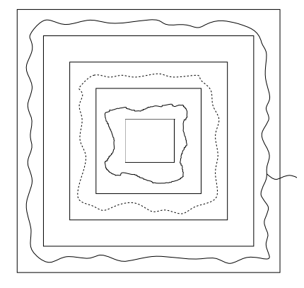
Figure 1: Illustration of the event $D_{k,m}$. The boxes, in order from smallest to largest, are $B(2^{k+1})$, $B(2^{k+1+\frac{m}{8}})$, $B(2^{k+1+\frac{m}{4}})$, $B(2^{k+1+\frac{m}{2}})$ and $B(2^{k+1+m})$. The solid circuit is $p_{c}$-open, the path to infinity is $p_{2^{k+1+\frac{m}{4}}}$-open, and the dotted path is $p_{2^{k+1+\frac{m}{4}}}$-closed.

For $j,k,m\geq 1$, we claim that

$$\left(\{R_{j}\geq 2^{k+1+m}\}\cap D_{k,m}\right)\subset\{r_{j}\geq 2^{k+1}\}.$$ (2.1.8)

To see why, suppose the left side occurs, and choose $\mathfrak{C}_{1}$ as a circuit from (i) in the definition of $D_{k,m}$, $\mathfrak{C}_{2}$ as a circuit from (ii), and $\mathfrak{C}_{3}$ as a circuit from (iii). Let $n_{1}$ be the time at which the invasion invades all of $\mathfrak{C}_{1}$ and for $i=2,3$, let $n_{i}$ be the first time that the invasion invades an edge from $\mathfrak{C}_{i}$. Note that $n_{1}\leq n_{2}\leq n_{3}\leq j$. (The last inequality holds because $R_{j}\geq 2^{k+1+m}$.)

After time $n_{3}$, the invasion has an unending supply of edges with weight $<p_{2^{k+1+\frac{m}{4}}}$ to invade, so it will never again take an edge with weight larger than that. Furthermore, at time $n_{2}$, the invasion must take an edge with weight larger than $p_{2^{k+1+\frac{m}{4}}}$. This implies that at some time $n_{4}\in[n_{2},n_{3})$, the invasion invades an outlet: an edge $\hat{e}$ such that all edges invaded after time $n_{4}$ have weight $<\omega(\hat{e})$. Furthermore, this outlet can be chosen to have weight $\omega(\hat{e})>p_{2^{k+1+\frac{m}{4}}}>p_{c}$.

Directly before time $n_{4}$, the entire boundary of the invasion (excluding $\hat{e}$ itself) consists of edges with weight $>\omega(\hat{e})$. Since invaded weights beyond time $n_{4}$ are $<\omega(\hat{e})$, none of these boundary edges will ever be invaded. Therefore all invaded edges after time $n_{4}$ are invaded through $\hat{e}$. In other words, if $e$ is any edge invaded after time $n_{4}$, there is a path $P(e)$ connecting $\hat{e}$ to $e$ consisting of edges with weight $<\omega(\hat{e})$ and which are invaded after time $n_{4}$. It is important to note that $P(e)$ cannot touch $\mathfrak{C}_{1}$. Indeed, if were to contain an edge $f$ which shared an endpoint with an edge on $\mathfrak{C}_{1}$ (including the possibility that $f\in\mathfrak{C}_{1}$), then $f$ would be accessible to the invasion at time $n_{1}$, and so $f$ would be invaded before time $n_{4}$, a contradiction.

Finally, to prove (2.1.8), assume that $r_{j}<2^{k+1}$. Then there is some time $j^{\prime}>j$ at which the invasion invades an edge $e$ in $B(2^{k+1})$. Since $j^{\prime}>n_{4}$, there is a path $P(e)$ from $\hat{e}$ to $e$ as in the preceding paragraph which cannot touch $\mathfrak{C}_{1}$. This means $\hat{e}$ is in the interior of $\mathfrak{C}_{1}$. On the other hand, if $f$ is any edge of $\mathfrak{C}_{3}$ (necessarily invaded after time $n_{4}$), the path $P(f)$ connecting $\hat{e}$ to $f$ would then toucn $\mathfrak{C}_{1}$, a contradiction. This shows (2.1.8).

Applying (2.1.8) for $C>0$ and $k,m\geq 1$, we obtain

$${\mathbb{P}}(r_{\lfloor C2^{2k}\pi(2^{k})\rfloor}<2^{k+1})\leq 2\max\{{\mathbb{P}}(R_{\lfloor C2^{2k}\pi(2^{k})\rfloor}<2^{k+1+m}),{\mathbb{P}}(D_{k,m}^{c}).\}$$ (2.1.9)

As in [4, proof of Thm. 5], the RSW theorem implies that $\mathbb{P}(D_{k,m}^{c})\leq e^{-\delta m}$ for some $\delta>0$ uniformly in $k$, so we can fix $m$ so that

$${\mathbb{P}}(D_{k,m}^{c})\leq\frac{\eta_{0}}{2}\text{ for all }k\geq 1.$$ (2.1.10)

From Lemma 2.1.1 and the fact that $\pi(n)$ is decreasing in $n$, for any $C\geq(2\mathcal{C}_{1}2^{2+2m})/\eta_{0}=:\mathcal{C}_{2}$, we get

$${\mathbb{P}}\big{(}R_{\lfloor C2^{2k}\pi(2^{k})\rfloor}<2^{k+1+m}\big{)} \leq{\mathbb{P}}\big{(}R_{\lfloor(2\mathcal{C}_{1}/\eta_{0})2^{2(k+1+m)}\pi(2^{k+1+m})\rfloor}<2^{k+1+m})\leq\frac{\eta_{0}}{2}.$$

Combining this with (2.1.9) and (2.1.10), we find that for $C\geq\mathcal{C}_{2}$,

$${\mathbb{P}}\big{(}r_{\lfloor C2^{2k}\pi(2^{k})\rfloor}<2^{k+1}\big{)}\leq\eta_{0},$$

and this completes the proof for $n$ of the form $2^{k}$.

For general $n$, we let $k=k(n):=\lfloor\log_{2}n\rfloor$, so that for any $C\geq 4\mathcal{C}_{2}$,

$${\mathbb{P}}(r_{\lfloor Cn^{2}\pi(n)\rfloor}<2n)\leq{\mathbb{P}}(r_{\lfloor\mathcal{C}_{2}2^{2(k+1)}\pi(2^{k+1})\rfloor}<2^{k+2})\leq\eta_{0}.$$

∎

2.2 Lower bound

In this section, we show that

$$\liminf_{n\to\infty}a_{n}(p_{c})>0.$$ (2.2.1)

The first step is to show that it suffices to prove this result for only a certain subsequence of values of $n$. Namely, we first prove that if there exists $\mathcal{C}_{3}>0$ such that

$$\liminf_{n\rightarrow\infty}a_{\lfloor\mathcal{C}_{3}n^{2}\pi(n)\rfloor}(p_{c})>0,$$ (2.2.2)

then (2.2.1) follows.

So assume that (2.2.2) holds, and let

$$k=k(n):=\max\{\ell:\mathcal{C}_{3}\ell^{2}\pi(\ell)\leq n\}.$$

(Note that this $k$ actually exists for large $n$ since $\pi(\ell)\geq D_{1}/\sqrt{\ell}$ by (2.1.5).) Since $\tilde{Q}_{n}(p_{c}+\epsilon)-\tilde{Q}_{n}(p_{c})$ is increasing in $n$,

$$\tilde{Q}_{n}(p_{c}+\epsilon)-\tilde{Q}_{n}(p_{c})\geq\tilde{Q}_{\lfloor\mathcal{C}_{3}k^{2}\pi(k)\rfloor}(p_{c}+\epsilon)-\tilde{Q}_{\lfloor\mathcal{C}_{3}k^{2}\pi(k)\rfloor}(p_{c}).$$

So using $n\leq L_{n}\leq 4n$, we obtain

$$\begin{split}a_{n}(p_{c})=\lim_{\epsilon\downarrow 0}\frac{{\mathbb{E}}[\tilde{Q}_{n}(p_{c}+\epsilon)-\tilde{Q}_{n}(p_{c})]}{\epsilon{\mathbb{E}}[L_{n}]}&\geq\displaystyle\lim_{\epsilon\downarrow 0}\frac{{\mathbb{E}}[\tilde{Q}_{\lfloor\mathcal{C}_{3}k^{2}\pi(k)\rfloor}(p_{c}+\epsilon)-\tilde{Q}_{\lfloor\mathcal{C}_{3}k^{2}\pi(k)\rfloor}(p_{c})]}{\epsilon{\mathbb{E}}[L_{\lfloor\mathcal{C}_{3}k^{2}\pi(k)\rfloor}]}\frac{{\mathbb{E}}[L_{\lfloor\mathcal{C}_{3}k^{2}\pi(k)\rfloor}]}{{\mathbb{E}}[L_{n}]}\\ &\geq a_{\lfloor\mathcal{C}_{3}k^{2}\pi(k)\rfloor}(p_{c})\frac{\mathcal{C}_{3}k^{2}\pi(k)}{8n}\\ \end{split}$$

Thus to conclude (2.2.1) from (2.2.2), it suffices to show that $\displaystyle\liminf_{n\rightarrow\infty}k^{2}\pi(k)/n$ is positive. For large $n$, $k(n)$ is greater than 1; therefore,

$$\frac{k^{2}\pi(k)}{n}\geq\frac{k^{2}\pi(k)}{\mathcal{C}_{3}(k+1)^{2}\pi(k+1)}\geq\mathcal{C}_{3}^{-1}\bigg{(}\frac{k}{k+1}\bigg{)}^{2}\geq\frac{1}{4\mathcal{C}_{3}}>0.$$

To prove (2.2.2), we use the following lemma, which bounds the $k^{th}$ moment of the number of edges of the IPC with $(p_{c},p_{c}+\epsilon]$ in $B(n)$.

Lemma 2.2.1.

Let $\mathcal{Y}_{n}(\epsilon)$ be the number of invaded edges in $B(n)$ with $(p_{c},p_{c}+\epsilon]$ for $\epsilon>0$. There exist positive constants $\mathcal{C}_{4}$ and $\mathcal{C}_{5}=\mathcal{C}_{5}(t)$ such that for all $n\geq 1$,

$$\liminf_{\epsilon\downarrow 0}\frac{{\mathbb{E}}|\mathcal{Y}_{n}(\epsilon)|}{\epsilon}\geq\mathcal{C}_{4}n^{2}\pi(n)$$

and

$${\mathbb{E}}|\mathcal{Y}_{n}(\epsilon)|^{t}\leq\mathcal{C}_{5}\left(\epsilon n^{2}\pi(n)\right)^{t}\text{ for all }t\geq 1\text{ and }\epsilon>0.$$

Assuming this lemma for the moment, we can derive (2.2.2). From Lemma 2.1.2, we can choose $\mathcal{C}_{3}$ so that

$${\mathbb{P}}(r_{\lfloor\mathcal{C}_{3}n^{2}\pi(n)\rfloor}<2n)\leq\frac{\mathcal{C}_{4}^{2}}{16\mathcal{C}_{5}(2)}\text{ for all }n\geq 1.$$

On the event $\{r_{\lfloor\mathcal{C}_{3}n^{2}\pi(n)\rfloor}\geq 2n\}$, the IPC in $B(2n)$ does not change after time $\lfloor\mathcal{C}_{3}n^{2}\pi(n)\rfloor$. It follows that the number of invaded edges with $(p_{c},p_{c}+\epsilon]$ until time $\lfloor\mathcal{C}_{3}n^{2}\pi(n)\rfloor$ is at least $\mathcal{Y}_{2n}(\epsilon)$, which is the number of invaded edges with $(p_{c},p_{c}+\epsilon]$ in $B(2n)$. By Lemma 2.1.2, Lemma 2.2.1 and the Cauchy-Schwarz inequality, if $\epsilon$ is sufficiently small,

$$\begin{split}{\mathbb{E}}\left[\displaystyle\sum_{j=1}^{\lfloor\mathcal{C}_{3}n^{2}\pi(n)\rfloor}\bigg{(}X_{j}(p_{c}+\epsilon)-X_{j}(p_{c})\bigg{)}\right]&\geq{\mathbb{E}}\left[\displaystyle\sum_{j=1}^{\lfloor\mathcal{C}_{3}n^{2}\pi(n)\rfloor}\bigg{(}X_{j}(p_{c}+\epsilon)-X_{j}(p_{c})\bigg{)}\cdot\mathbf{1}_{\{r_{\lfloor\mathcal{C}_{3}n^{2}\pi(n)\rfloor}\geq 2n\}}\right]\\ &\geq{\mathbb{E}}\left[\mathcal{Y}_{2n}(\epsilon)\cdot\mathbf{1}_{\{r_{\lfloor\mathcal{C}_{3}n^{2}\pi(n)\rfloor}\geq 2n\}}\right]\\ &\geq\frac{\mathcal{C}_{4}}{2}\epsilon(2n)^{2}\pi(2n)-{\mathbb{E}}\left[\mathcal{Y}_{2n}(\epsilon)\cdot\mathbf{1}_{\{r_{\lfloor\mathcal{C}_{3}n^{2}\pi(n)\rfloor}<2n\}}\right]\\ &\geq\frac{\mathcal{C}_{4}}{2}\epsilon(2n)^{2}\pi(2n)-\sqrt{\mathcal{C}_{5}(2)\left(\epsilon(2n)^{2}\pi(2n)\right)^{2}\frac{\mathcal{C}_{4}^{2}}{16\mathcal{C}_{5}(2)}}\\ &\geq\frac{\mathcal{C}_{4}\epsilon(2n)^{2}\pi(2n)}{4}.\end{split}$$

Combining this with (1.2.2), (2.1.5), and the fact that $n\leq{\mathbb{E}}[L_{n}]\leq 4n$, we obtain

$$\begin{split}a_{\lfloor\mathcal{C}_{3}n^{2}\pi(n)\rfloor}(p_{c})=\displaystyle\lim_{\epsilon\downarrow 0}\frac{{\mathbb{E}}[\tilde{Q}_{\lfloor\mathcal{C}_{3}n^{2}\pi(n)\rfloor}(p_{c}+\epsilon)-\tilde{Q}_{\lfloor\mathcal{C}_{3}n^{2}\pi(n)\rfloor}(p_{c})]}{\epsilon{\mathbb{E}}[L_{\lfloor\mathcal{C}_{3}n^{2}\pi(n)\rfloor}]}&\geq\displaystyle\lim_{\epsilon\downarrow 0}\frac{\mathcal{C}_{4}\epsilon(2n)^{2}\pi(2n)/4}{4\epsilon\mathcal{C}_{3}n^{2}\pi(n)}\\ &=\frac{\mathcal{C}_{4}D_{1}}{4\mathcal{C}_{3}\sqrt{2}},\end{split}$$

which is positive uniformly in $n$. This shows (2.2.2).

The last step is to prove Lemma 2.2.1.

Proof of Lemma 2.2.1.

The proof of the upper bound is similar to that of Járai [10, Theorem 1], which shows an upper bound for $|\mathcal{S}_{n}|$ (that result does not involve a condition on the weight $\omega(e)$) so we will omit some details. We will follow that proof, but make the events independent of $\omega(e)$ so that we can insert the condition $\omega(e)\in(p_{c},p_{c}+\epsilon]$.

We will restrict to $n$ of the form $2^{K}$, as the general result follows from this and monotonicity of $\pi_{n}$. Let $A_{k}$ be Ann($2^{k},2^{k+1})$, and $\mathcal{Y}_{A_{k}}$ be the number of IPC edges in Ann($2^{k},2^{k+1})$ with the weight in $(p_{c},p_{c}+\epsilon]$. Then, $B(n)=\cup_{k=1}^{K}A_{k}$ and $\mathcal{Y}_{n}(\epsilon)=\sum_{k=1}^{K}\mathcal{Y}_{A_{k}}$. Define a sequence $p_{k}(0)>p_{k}(1)>\cdots>p_{c}$ as follows. Let $\log^{(0)}k=k$, and let $\log^{(j)}k=\log(\log^{(j-1)}k)$ for $j\geq 1$ if the right-hand side is defined. For $k>10$, we define

$$\log^{*}k=\min\{j>0:\log^{(j)}k\;\text{ is defined and }\log^{(j)}k\leq 10\}.$$

Then $\log^{(j)}k>2$, for $j=0,1,\cdots,\log^{*}k$ and $k>10$. Let

$$p_{k}(j)=\inf\left\{p>p_{c}:L(p)\leq\frac{2^{k}}{C_{5}\log^{(j)}k}\right\},\;\;j=0,1,\cdots,\log^{*}k,$$

where the constant $C_{5}$ will be chosen later. With (2.1.4) and [10, Eq. (2.15)], we get

$$C_{5}\log^{(j)}k\leq\frac{2^{k}}{L(p_{k}(j))}\leq DC_{5}\log^{(j)}k$$ (2.2.3)

For any fixed $e\subset A_{k}$ we define

$$H_{k}(j)=\{\text{$\exists$ a $p_{k}(j)$-open circuit $\mathcal{D}$ around the origin in $A_{k-1}$ and $\mathcal{D}\ext@arrow 9999{\arrowfill@\leftarrow\relbar\rightarrow}{}{p_{k}(j)}\infty$}\}$$

$$H^{e}_{k}(j)=\{\text{$H_{k}(j)$ occurs and $\mathcal{D}\ext@arrow 9999{\arrowfill@\leftarrow\relbar\rightarrow}{}{\;p_{k}(j)\;}\infty$ without using the edge $e$}\}.$$ (2.2.4)

To give a lower bound for the probability of $H_{k}(j)$, Járai constructed an infinite $p_{k}(j)$-open path starting from $\partial B(2^{k})$ using standard 2D constructions only to the right of $B(2^{k})$. (See [10, Fig 1]). Similarly, to lower bound the probability of $H_{k}(j)^{e}$, we build, in addition to Járai’s path, an infinite $p_{k}(j)$-open path starting from $\partial B(2^{k})$ in the left of $B(2^{k})$. The existence of such disjoint two infinite $p_{k}(j)$-open paths imply the event $\{\mathcal{D}\ext@arrow 9999{\arrowfill@\leftarrow\relbar\rightarrow}{}{\;p_{k}(j)\;}\infty\text{ without using $e$}\}$ for any fixed edge $e\in A_{k}$. As in [10, Eq. (2.17)], we obtain

$$J_{k}(j)\cap\bigg{(}\bigcap_{m=0}^{\infty}J_{k,L}^{m}(j)\bigg{)}\cap\bigg{(}\bigcap_{m=0}^{\infty}J_{k,R}^{m}(j)\bigg{)}\subseteq H^{e}_{k}(j)$$ (2.2.5)

where for $m\geq 0$,

$$\begin{split}&J_{k}=\{\text{$\exists$ a $p_{k}(j)$-open circuit in $A_{k-1}$}\}\\ &J_{k,R}^{m}=J_{k,R}^{m,h}\cap J_{k,R}^{m,v},\;\text{and}\;J_{k,L}^{m}=J_{k,L}^{m,h}\cap J_{k,L}^{m,v}\\ &J_{k,R}^{m,h}=\{\text{$\exists$ a $p_{k}(j)$-open horizontal crossing of $[2^{k-2+m},2^{k+m}]\times[-2^{k-2+m},2^{k-2+m}]$}\}\\ &J_{k,L}^{m,h}=\{\text{$\exists$ a $p_{k}(j)$-open horizontal crossing of $[-2^{k+m},-2^{k-2+m}]\times[-2^{k-2+m},2^{k-2+m}]$}\}\\ &J_{k,R}^{m,v}=\{\text{$\exists$ a $p_{k}(j)$-open vertical crossing of $[2^{k-1+m},2^{k+m}]\times[-2^{k-1+m},2^{k-1+m}]$}\}\\ &J_{k,L}^{m,v}=\{\text{$\exists$ a $p_{k}(j)$-open vertical crossing of $[-2^{k+m},-2^{k-1+m}]\times[-2^{k-1+m},2^{k-1+m}]$}\}.\\ \end{split}$$

By (2.1.3) and (2.2.3), (See [10, Eqs. (2.19), (2.20)]),

$$\begin{split}&{\mathbb{P}}(J_{k}(j)^{c})\leq 16C_{3}\exp\left\{-\frac{1}{4}C_{4}C_{5}\log^{(j)}k\right\}\;\;\text{ and }\\ &{\mathbb{P}}(J_{k,R}^{m}(j)^{c}\cup J_{k,L}^{m}(j)^{c})\leq 4C_{3}\exp\left\{-\frac{1}{2}C_{4}C_{5}2^{m}\log^{(j)}k\right\}.\end{split}$$

By these inequalities, one gets

$${\mathbb{P}}(H_{k}^{e}(j)^{c}) \leq{\mathbb{P}}\left(J_{k}(j)\right)^{c}+\displaystyle\sum_{m=0}^{\infty}{\mathbb{P}}\left((J_{k,R}^{m}(j)^{c}\cup J_{k,L}^{m}(j)^{c}\right)$$

$$\leq(16C_{3}+C_{6})\exp\left\{-\frac{1}{4}C_{4}C_{5}\log^{(j)}k\right\}.$$

We write $C_{7}$ as $16C_{3}+C_{6}$ and $c_{1}$ as $\frac{C_{4}C_{5}}{4}$ for short. Then,

$${\mathbb{P}}(H_{k}^{e}(j)^{c})\leq C_{7}\exp\{-c_{1}\log^{(j)}k\}.$$ (2.2.6)

The constant $c_{1}$ can be made large by choosing $C_{5}$ large.

To estimate the mean of $\mathcal{Y}_{A_{k}}$, we decompose

$${\mathbb{E}}\mathcal{Y}_{A_{k}}={\mathbb{E}}\left[\mathcal{Y}_{A_{k}};H_{k}(0)^{c}\right]+\bigg{(}\displaystyle\sum_{j=1}^{\log^{*}k}{\mathbb{E}}\left[\mathcal{Y}_{A_{k}};H_{k}(j-1)\cap H_{k}(j)^{c}\right]\bigg{)}+{\mathbb{E}}\left[\mathcal{Y}_{A_{k}};H_{k}(\log^{*}k)\right].$$ (2.2.7)

By (2.2.6) and independence,

$$\begin{split}{\mathbb{E}}\left[\mathcal{Y}_{A_{k}};H_{k}(0)^{c}\right]&\leq{\mathbb{E}}\left[\mathcal{Y}_{A_{k}};H_{k}^{e}(0)^{c}\right]\leq\displaystyle\sum_{e\in A_{k}}{\mathbb{P}}(\omega(e)\in(p_{c},p_{c}+\epsilon],H_{k}^{e}(0)^{c})\\ &=|A_{k}|{\mathbb{P}}(\omega(e)\in(p_{c},p_{c}+\epsilon]){\mathbb{P}}(H_{k}^{e}(0)^{c})\\ &\leq|A_{k}|\epsilon C_{8}e^{-c_{1}k}.\end{split}$$ (2.2.8)

Next, since $\omega(e)$ is independent of $H_{k}^{e}(j)\cap\{e\ext@arrow 9999{\arrowfill@\leftarrow\relbar\rightarrow}{}{p_{k}(j)}\infty\}$,

$$\begin{split}{\mathbb{E}}|\mathcal{Y}_{A_{k}};H_{k}(j-1)\cap H_{k}(j)^{c}|&=\displaystyle\sum_{e\in A_{k}}{\mathbb{P}}(\omega(e)\in(p_{c},p_{c}+\epsilon]\cap\{e\ext@arrow 9999{\arrowfill@\leftarrow\relbar\rightarrow}{}{p_{k}(j-1)}\infty\}\cap H_{k}^{e}(j)^{c})\\ &=\epsilon\displaystyle\sum_{e\in A_{k}}{\mathbb{P}}(e\ext@arrow 9999{\arrowfill@\leftarrow\relbar\rightarrow}{}{p_{k}(j-1)}\infty,H_{k}^{e}(j)^{c}).\end{split}$$

Applying the FKG inequality and (2.2.6) to this, we obtain

$$\begin{split}{\mathbb{E}}[\mathcal{Y}_{A_{k}};H_{k}(j-1)\cap H_{k}(j)^{c}]\leq|A_{k}|\epsilon\theta(p_{k}(j-1))\;C_{7}\exp\{-c_{1}\log^{(j)}k\}.\\ \end{split}$$ (2.2.9)

The third term of (2.2.7) is bounded above by

$$|A_{k}|\epsilon\theta(p_{k}(\log^{*}k)).$$ (2.2.10)

Using (2.1.2), (2.1.5) and (2.2.3),

$$\theta(p_{k}(j))\leq\frac{\pi(2^{k})}{D_{1}}(DC_{5}\log^{(j)}k)^{1/2}.$$

Applying this inequality after placing (2.2.8), (2.2.9), and (2.2.10) into (2.2.7), we obtain

$$\begin{split}{\mathbb{E}}\mathcal{Y}_{A_{k}}\leq C_{9}|A_{k}|\epsilon\pi(2^{k})\left[\frac{\exp\{-c_{1}k\}}{\pi(2^{k})}+\left\{\displaystyle\sum_{j=1}^{\log^{*}k}(\log^{j-1}k)^{1/2-c_{1}}\right\}+1\right].\end{split}$$

Since $\pi(2^{k})\geq C_{10}2^{-k/2}$ from (2.1.5), we can choose $C_{5}$ (and therefore $c_{1}$) so large that

$$\frac{\exp\{-c_{1}k\}}{\pi(2^{k})}+\left\{\displaystyle\sum_{j=1}^{\log^{*}k}(\log^{j-1}k)^{1/2-c_{1}}\right\}+1\;\;\text{ is bounded in $k$,}$$

and so ${\mathbb{E}}\mathcal{Y}_{A_{k}}\leq C_{11}\epsilon 2^{2k}\pi(2^{k}).$ Recalling $n=2^{K}$, we obtain from this and (2.1.5) that

$$\begin{split}{\mathbb{E}}\mathcal{Y}_{n}(\epsilon)=\displaystyle\sum_{k=1}^{K}{\mathbb{E}}\mathcal{Y}_{A_{k}}\leq C_{11}\epsilon 2^{2K}\pi(2^{K})\displaystyle\sum_{k=1}^{K}\frac{2^{2k}\pi(2^{k})}{2^{2K}\pi(2^{K})}&\leq\frac{C_{11}}{D_{1}}\epsilon 2^{2K}\pi(2^{K})\displaystyle\sum_{k=1}^{K}2^{2(k-K)}2^{-\frac{1}{2}(k-K)}\\ &\leq C_{12}\epsilon n^{2}\pi(n),\end{split}$$

completing the proof of the upper bound when $t=1$. The extension to larger $t$ uses the same ideas as in [10] and [11, Sec. 3], so we omit it.

We now turn to the lower bound. For $k\geq 1$, $\epsilon>0$, and any $e\subset A_{k}$, we let $L_{k}(e)$ be the event that the following hold:

1. There exists a $p_{c}$-open circuit $\mathcal{D}$ around the origin in $A_{k-2}$.

2. There exists a $(p_{c}+\epsilon)$-closed dual circuit around the origin in $A_{k+2}$.

3. $\mathcal{D}$ is connected to the edge $e\in A_{k}$ by a $p_{c}$-open path in $B(2^{k})$.

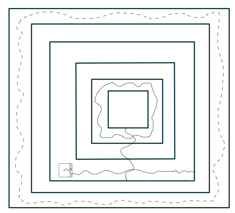
Figure 2: The event $L_{k}(e)$. The boxes, in order from smallest to largest, are $B(2^{k-2})$, $B(2^{k-1})$, $B(2^{k})$, $B(2^{k+1})$, $B(2^{k+2})$, and $B(2^{k+3})$. The solid curves are $p_{c}$-open and the dotted curve is a $(p_{c}+\epsilon)$-closed dual circuit.

(See Figure 2 for an illustration of $L_{k}(e)$).

If the events described in (a) and (b) both occur, each $(p_{c}+\epsilon)$-open edge connected to $\mathcal{D}$ by a $(p_{c}+\epsilon)$-open path will eventually be invaded. Since the event in (b) depends on edge-variables for edges outside of $B(2^{k+1})$, (b) is independent of both (a) and (c). In addition, the events (a) and (c) are increasing. So, by the FKG inequality and the RSW theorem,

$${\mathbb{P}}(L_{k}(e))\geq{\mathbb{P}}((a))\times{\mathbb{P}}((b))\times{\mathbb{P}}((c))\geq C_{13}{\mathbb{P}}((b))\times{\mathbb{P}}((c)).$$

By a gluing argument [8, Ch. 11] using the FKG inequality and the RSW theorem, ${\mathbb{P}}((c))\geq C_{14}\pi(2^{k})$. Furthermore, as long as $\epsilon$ is so small that $p_{c}+\epsilon<p_{2^{k+2}}$, then the RSW theorem implies that ${\mathbb{P}}((b))\geq C_{15}$. This means that for such $\epsilon$, one has ${\mathbb{P}}(L_{k}(e))\geq C_{13}C_{14}C_{15}\pi(2^{k})$. Since $\omega(e)$ and the event $L_{k}(e)$ are independent,

$$\begin{split}{\mathbb{E}}|\mathcal{Y}_{A_{k}}|=\displaystyle\sum_{e\in A_{k}}{\mathbb{P}}(e\in\text{IPC},\omega(e)\in(p_{c},p_{c}+\epsilon])&\geq\displaystyle\sum_{e\in A_{k}}{\mathbb{P}}(L_{k}(e),\omega(e)\in(p_{c},p_{c}+\epsilon])\\ &\geq C_{16}\epsilon 2^{2k}\pi(2^{k}).\end{split}$$

For a given $n\geq 1$, choose $k=\lfloor\log_{2}n\rfloor$ to complete the proof:

$${\mathbb{E}}\mathcal{Y}_{n}(\epsilon)\geq{\mathbb{E}}\mathcal{Y}_{A_{k}}\geq C_{16}\epsilon 2^{2k}\pi(2^{k})\geq C_{17}\epsilon n^{2}\pi(n).$$

∎

2.3 Upper bound

In this section, we show that

$$\limsup_{n\to\infty}a_{n}(p_{c})<1.$$ (2.3.1)

To prove (2.3.1), we define

$$\Xi_{n}(\epsilon)=\left[\tilde{P}_{n}(p_{c}+\epsilon)-\tilde{P}_{n}(p_{c})\right]-\left[\tilde{Q}_{n}(p_{c}+\epsilon)-\tilde{Q}_{n}(p_{c})\right],$$

as the number of edges with weight in the interval $(p_{c},p_{c}+\epsilon]$ which the invasion observes until time $n$ but does not invade, and we give the following proposition.

Proposition 2.1.

There exists $\mathcal{C}_{6}>0$ and a function $G$ on $[0,\infty)$ with $\inf_{r\in[0,m]}G(r)>0$ for each $m\geq 0$ such that for any $C\geq\mathcal{C}_{6}$, any $n\geq 1$, and any $\epsilon>0$,

$${\mathbb{E}}\Xi_{\lfloor Cn^{2}\pi(n)\rfloor}(\epsilon)\geq G(C)\epsilon n^{2}\pi(n).$$

Assuming Proposition 2.1 for the moment, let $C\geq\mathcal{C}_{6}$, and use $\mathbb{E}L_{n}\leq 4n$ for

$$a_{\lfloor Cn^{2}\pi(n)\rfloor}(p_{c})=\displaystyle\lim_{\epsilon\downarrow 0}\frac{{\mathbb{E}}\left[\tilde{Q}_{\lfloor Cn^{2}\pi(n)\rfloor}(p_{c}+\epsilon)-\tilde{Q}_{\lfloor Cn^{2}\pi(n)\rfloor}(p_{c})\right]}{{\mathbb{E}}\left[\tilde{P}_{\lfloor Cn^{2}\pi(n)\rfloor}(p_{c}+\epsilon)-\tilde{P}_{\lfloor Cn^{2}\pi(n)\rfloor}(p_{c})\right]} =\displaystyle\lim_{\epsilon\downarrow 0}\left(1-\frac{{\mathbb{E}}\Xi_{\lfloor Cn^{2}\pi(n)\rfloor}(\epsilon)}{{\mathbb{E}}L_{\lfloor Cn^{2}\pi(n)\rfloor}}\right)$$

$$\leq\displaystyle\lim_{\epsilon\downarrow 0}\bigg{(}1-\frac{G(C)\epsilon n^{2}\pi(n)}{4C\epsilon n^{2}\pi(n)}\bigg{)}$$

$$=1-\frac{G(C)}{4C}.$$ (2.3.2)

Now note that any $n\geq\mathcal{C}_{6}$ can be written in the form $\lfloor Ch^{2}\pi(h)\rfloor$ for some integer $h\geq 1$ and some $C\in[\mathcal{C}_{6},4\mathcal{C}_{6}]$. To see why, observe that any $n\geq\mathcal{C}_{6}$ is in some interval of the form $[\mathcal{C}_{6}h^{2}\pi(h),\mathcal{C}_{6}(h+1)^{2}\pi(h+1))$ for some $h\geq 1$ (since $h^{2}\pi(h)\to\infty$ as $h\to\infty$ by (2.1.5)). Then because

$$\frac{\mathcal{C}_{6}(h+1)^{2}\pi(h+1)}{\mathcal{C}_{6}h^{2}\pi(h)}=\left(1+\frac{1}{h}\right)^{2}\frac{\pi(h+1)}{\pi(h)}\leq 4,$$

we see that $n=\lfloor C_{\ast}\mathcal{C}_{6}h^{2}\pi(h)\rfloor$ for some $C_{\ast}\in[1,4]$. By (2.3.2), then, we obtain

$$a_{n}(p_{c})\leq 1-\frac{\inf_{r\in[\mathcal{C}_{6},4\mathcal{C}_{6}]}G(r)}{4\mathcal{C}_{6}},$$

and this implies (2.3.1).

In the remainder of this section, we prove Proposition 2.1.

Proof of Proposition 2.1.

For notational convenience, let $t_{n}=\lfloor Cn^{2}\pi(n)\rfloor$. To prove a lower bound on $\Xi_{t_{n}}(\epsilon)$, we will construct a large $p_{c}$-open cluster such that with positive probability, independent of $n$, the invasion has intersected this cluster at time $t_{n}$ and has explored a positive fraction of its boundary edges, but has not yet absorbed the entire cluster. These explored boundary edges will have probability of order $\epsilon$ to have weight in the interval $(p_{c},p_{c}+\epsilon]$, so our lower bound on ${\mathbb{E}}\Xi_{t_{n}}(\epsilon)$ will be of order $\epsilon$ times the size of this explored boundary, which will itself be of order $n^{2}\pi(n)$.

To construct this cluster, we need several definitions.

Definition 2.2.

Define the event $D(n)$ that the following conditions hold:

1. There exists a $q_{n}$-open circuit around the origin in Ann($n,2n$).

2. There exists an edge $f\in$ Ann$(6n,7n)$ with $\omega(f)\in(q_{n},p_{c})$ such that:

   1. there exists a $p_{c}$-closed dual path $P$ around the origin in Ann($4n,8n)^{*}\backslash\{f^{*}\}$ that is connected to the endpoints of $f^{*}$ so that $P\cup\{f^{*}\}$ is a dual circuit around the origin, and

   2. there exists a $p_{c}$-open path connecting an endpoint of $f$ to $B(n)$, and another disjoint $p_{c}$-open path connecting the other endpoint of $f$ to $\partial B(16n)$.

3. There exists a $p_{c}$-open circuit around the origin in Ann($8n,16n)$.

For $e\subset Ann(2n,4n)$, define $D^{e}(n)$ as the event that $D(n)$ occurs without using the edge $e$. (That is, $D(n)$ occurs and the first connection listed in 2(b) does not use $e$.)

See Figure 3 for an illustration of $D(n)$.

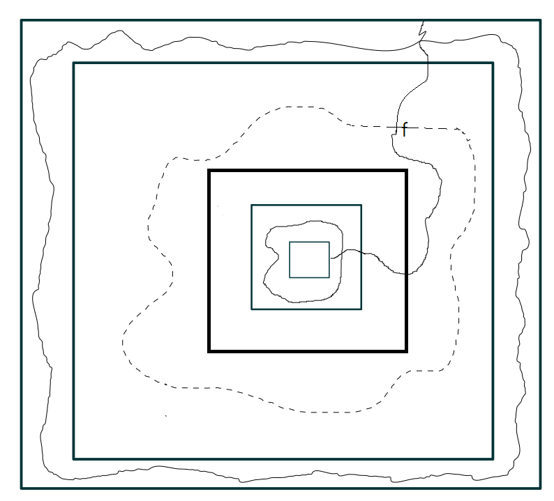
Figure 3: The event $D(n)$. The boxes, in order from smallest to largest, are $B(n)$, $B(2n)$, $B(4n)$, $B(8n)$ and $B(16n)$. The solid circuit in Ann($n,2n$) is $q_{n}$-open and the path from $\partial B(n)$ to $f$ is $p_{c}$-open; the dotted dual path in Ann($4n,8n$) is $p_{c}$-closed, $\omega(f)\in(q_{n},p_{c})$, and the other solid paths are $p_{c}$-open.

When the event $D(n)$ occurs, we can define $\mathcal{C}_{\ast}$ as the innermost $q_{n}$-open circuit around the origin in $Ann(n,2n)$ and $D_{\ast}$ as the outermost $p_{c}$-open circuit around the origin in $Ann(8n,16n)$. Note that on $D(n)$, the circuits $\mathcal{C}_{\ast}$ and $D_{\ast}$ are part of the same $p_{c}$-open cluster; this will form part of our “large cluster” referenced above. We need to make sure that we have started to invade this cluster, but are not yet done at time $t_{n}$, so we define stopping times

$$t_{D_{\ast}} =\text{ first time at which the invasion invades an edge from $D_{\ast}$}$$

$$T_{D_{\ast}} =\text{ first time at which the invasion invades the entire $p_{c}$-open cluster of $D_{\ast}$}.$$

Note that on $D(n)$, we have $t_{D_{\ast}}\leq T_{D_{\ast}}$ and trivially,

$${\mathbb{E}}\Xi_{t_{n}}(\epsilon)\geq{\mathbb{E}}\Xi_{t_{n}}(\epsilon)\mathbf{1}_{D(n)\cap\{t_{D_{\ast}}\leq t_{n}<T_{D_{\ast}}\}}.$$ (2.3.3)

The next lemma shows that on the events listed on the right, $\Xi_{t_{n}}(\epsilon)$ is, on average, at least order $\epsilon$ times the cardinality of a certain subset of the edge boundary of the $p_{c}$-open cluster of $D_{\ast}$. For this we define the size $Y_{n}$ of this subset:

$$Y_{n}=\#\{e\subset Ann(2n,4n):\omega(e)>p_{c},e\ext@arrow 9999{\arrowfill@\leftarrow\relbar\rightarrow}{}{q_{n}}\partial B(n)\text{ in }B(4n)\}.$$

Lemma 2.3.1.

For any $n\geq 1$,

$${\mathbb{E}}\Xi_{t_{n}}(\epsilon)\mathbf{1}_{D(n)\cap\{t_{D_{\ast}}\leq t_{n}<T_{D_{\ast}}\}}\geq\frac{\epsilon}{1-p_{c}}{\mathbb{E}}Y_{n}\mathbf{1}_{D(n)\cap\{t_{D_{\ast}}\leq t_{n}<T_{D_{\ast}}\}}.$$

Proof.

First we let

$$\hat{Y}_{n}=\#\{e\subset Ann(2n,4n):\omega(e)\in(p_{c},p_{c}+\epsilon],e\ext@arrow 9999{\arrowfill@\leftarrow\relbar\rightarrow}{}{q_{n}}\partial B(n)\text{ in }B(4n)\}.$$

On the event $D(n)\cap\{t_{D_{\ast}}\leq t_{n}<T_{D_{\ast}}\}$, any edge in the set which defines $\hat{Y}_{n}$ will be observed by the invasion until time $t_{n}$ but will not be invaded (that is, it is counted in the definition of $\Xi_{n}(\epsilon)$). To see why, let $e$ be an edge in the set which defines $\hat{Y}_{n}$. First, we must show that $e$ is not invaded at time $t_{n}$. This is because, in order for the invasion to even observe $e$, it must first pass through the circuit $\mathcal{C}_{\ast}$. Since $\omega(e)>p_{c}$, the invasion will invade the entire $p_{c}$-open cluster of $\mathcal{C}_{\ast}$ (which equals the $p_{c}$-open cluster of $D_{\ast}$) before it invades $e$. Since $t_{n}<T_{D_{\ast}}$, $e$ cannot be invaded at time $t_{n}$. Second, we must show that $e$ is observed by time $t_{n}$. The reason is that since $t_{D_{\ast}}\leq t_{n}$, at time $t_{n}$, the invasion has already invaded an edge from $D_{\ast}$. Since $D(n)$ occurs, the edge $f$ must therefore be invaded before time $t_{D_{\ast}}\leq t_{n}$. Before $f$ can be invaded, the entire $q_{n}$-open cluster of $\mathcal{C}_{\ast}$ must be invaded, so at least one endpoint of $e$ is in the invasion at time $t_{n}$. This means that $e$ is observed by time $t_{n}$. In conclusion,

$${\mathbb{E}}\Xi_{t_{n}}(\epsilon)\mathbf{1}_{D(n)\cap\{t_{D_{\ast}}\leq t_{n}<T_{D_{\ast}}\}}$$

$$\geq~{} {\mathbb{E}}\hat{Y}_{n}\mathbf{1}_{D(n)\cap\{t_{D_{\ast}}\leq t_{n}<T_{D_{\ast}}\}}$$

$$=~{} \sum_{e\subset\text{Ann}(2n,4n)}\mathbb{P}(\omega(e)\in(p_{c},p_{c}+\epsilon],e\ext@arrow 9999{\arrowfill@\leftarrow\relbar\rightarrow}{}{q_{n}}\partial B(n)\text{ in }B(4n),D(n),t_{D_{\ast}}\leq t_{n}<T_{D_{\ast}}).$$

The second and final step is to show that for all $e\subset\text{Ann}(2n,4n)$, we have

$$\begin{split}&\mathbb{P}(\omega(e)\in(p_{c},p_{c}+\epsilon],e\ext@arrow 9999{\arrowfill@\leftarrow\relbar\rightarrow}{}{q_{n}}\partial B(n)\text{ in }B(4n),D(n),t_{D_{\ast}}\leq t_{n}<T_{D_{\ast}})\\ =~{}&\frac{\epsilon}{1-p_{c}}\mathbb{P}(\omega(e)>p_{c},e\ext@arrow 9999{\arrowfill@\leftarrow\relbar\rightarrow}{}{q_{n}}\partial B(n)\text{ in }B(4n),D(n),t_{D_{\ast}}\leq t_{n}<T_{D_{\ast}}).\end{split}$$ (2.3.4)

Once this is done, we can sum the right side and obtain the statement of the lemma.

To argue for (2.3.4), we need to be able to decouple the value of $\omega(e)$ from the other events. Intuitively this should be possible because when $D(n)$ occurs, after the invasion touches $\mathcal{C}_{\ast}$, it does not need to check any weights for edges which are $p_{c}$-closed until after time $T_{D_{\ast}}$. To formally prove this, we represent the weights $(\omega(e))$ used for the invasion as functions of three independent variables. This representation is used in the “percolation cluster method” of Chayes-Chayes-Newman, but their method uses them in a dynamic way, whereas ours will be static. For this representation, we assign different variables to the edges: let $(U_{e}^{1},U_{e}^{2},\eta_{e})_{e\in\mathcal{E}^{2}}$ be an i.i.d. family of independent variables, where $U_{e}^{1}$ is uniform on $[0,p_{c}]$, $U_{e}^{2}$ is uniform on $(p_{c},1]$, and $\eta_{e}$ is Bernoulli with parameter $p_{c}$. Then we set

$$\omega(e)=\begin{cases}U_{e}^{1}&\quad\text{if }\eta_{e}=1\\ U_{e}^{2}&\quad\text{if }\eta_{e}=0.\end{cases}$$

Next, we define another invasion percolation process $(\hat{G}_{n})$ (a sequence of growing subgraphs) as follows. If $D(n)$ does not occur, then $\hat{G}_{n}$ is equal to $(0,\{\})$ for all $n$ (it stays at the origin with no edges). If $D(n)$ does occur, then $\hat{G}_{n}$ proceeds according to the usual invasion rules (with the weights $(\omega(e))$) until it reaches $\mathcal{C}_{\ast}$. After it contains a vertex of $\mathcal{C}_{\ast}$, it no longer checks the $\omega$-value of any edge $\hat{e}$ with $\eta_{\hat{e}}=0$ (it only checks the $\eta$-value). When there are no more edges with $\eta$-value equal to one for the invasion to invade, it stops (we set $\hat{G}_{n}$ to be constant after this time). Associated to this new invasion will be stopping times similar to $t_{D_{\ast}}$ and $T_{D_{\ast}}$:

$$\hat{t}_{D_{\ast}} =\text{ first time at which the new invasion invades an edge from $D_{\ast}$}$$

$$\hat{T}_{D_{\ast}} =\text{ first time at which the new invasion invades the entire $p_{c}$-open cluster of $D_{\ast}$}.$$

Note that if $D(n)$ does not occur, $\hat{t}_{D_{\ast}}=\hat{T}_{D_{\ast}}=\infty$, and that if $D(n)$ occurs, $\hat{T}_{D_{\ast}}$ equals the first time after which the graphs $\hat{G}_{n}$ become constant.

Given these definitions, the top equation of (2.3.4) equals

$$\mathbb{P}(U_{e}^{2}\in(p_{c},p_{c}+\epsilon],\eta_{e}=0,e\ext@arrow 9999{\arrowfill@\leftarrow\relbar\rightarrow}{}{q_{n}}\partial B(n)\text{ in }B(4n),D(n),t_{D_{\ast}}\leq t_{n}<T_{D_{\ast}}).$$

We then claim that

$$\begin{split}&\mathbb{P}(U_{e}^{2}\in(p_{c},p_{c}+\epsilon],\eta_{e}=0,e\ext@arrow 9999{\arrowfill@\leftarrow\relbar\rightarrow}{}{q_{n}}\partial B(n)\text{ in }B(4n),D(n),t_{D_{\ast}}\leq t_{n}<T_{D_{\ast}})\\ =~{}&\mathbb{P}(U_{e}^{2}\in(p_{c},p_{c}+\epsilon],\eta_{e}=0,e\ext@arrow 9999{\arrowfill@\leftarrow\relbar\rightarrow}{}{q_{n}}\partial B(n)\text{ in }B(4n),D(n),\hat{t}_{D_{\ast}}\leq t_{n}<\hat{T}_{D_{\ast}}).\end{split}$$ (2.3.5)

This equation holds because when $D(n)$ occurs, $t_{D_{\ast}}=\hat{t}_{D_{\ast}}$ and $T_{D_{\ast}}=\hat{T}_{D_{\ast}}$. Indeed, if $D(n)$ occurs, then both invasions $(G_{n})$ and $(\hat{G}_{n})$ are equal until they touch $\mathcal{C}_{\ast}$. After this time, the original invasion $(G_{n})$ does not invade any $p_{c}$-closed edges until time $T_{D_{\ast}}$, and neither does $(\hat{G}_{n})$ (by definition). This shows (2.3.5).

Now that we have (2.3.5), we simply note that because $(\hat{G}_{n})$ does not use any edges in $B(2n)^{c}$ that are $p_{c}$-closed, the the times $\hat{t}_{D_{\ast}}$ and $\hat{T}_{D_{\ast}}$ are independent of $(U_{e}^{2})_{e\in B(2n)^{c}}$. Furthermore, the events $\{\eta_{e}=0\}$, $\{e\ext@arrow 9999{\arrowfill@\leftarrow\relbar\rightarrow}{}{q_{n}}\partial B(n)\text{ in }B(4n)\}$, and $D(n)$ are independent of $(U_{e}^{2})_{e\in B(2n)^{c}}$, and $U_{e}^{2}\in(p_{c},p_{c}+\epsilon]$ depends only on $(U_{e}^{2})_{e\in B(2n)^{c}}$. By independence, therefore, the lower equation of (2.3.5) is equal to

$$\frac{\epsilon}{1-p_{c}}\mathbb{P}(\eta_{e}=0,e\ext@arrow 9999{\arrowfill@\leftarrow\relbar\rightarrow}{}{q_{n}}\partial B(n)\text{ in }B(4n),D(n),\hat{t}_{D_{\ast}}\leq t_{n}<\hat{T}_{D_{\ast}}),$$

which equals the bottom equation in (2.3.4). This shows (2.3.4). ∎

Combining Lemma 2.3.1 with (2.3.3), and then reducing to the subevent $D^{e}(n)$ (recall this is the subevent of $D(n)$ on which the paths involved in $D(n)$ do not use the given $e\subset$ Ann$(2n,4n)$), we obtain

$${\mathbb{E}}\Xi_{t_{n}}$$

$$\geq~{} \frac{\epsilon}{1-p_{c}}{\mathbb{E}}Y_{n}\mathbf{1}_{D(n)\cap\{t_{D_{\ast}}\leq t_{n}<T_{D_{\ast}}\}}$$

$$\geq~{} \frac{\epsilon}{1-p_{c}}\sum_{e\subset\text{Ann}(2n,4n)}\mathbb{P}(\omega(e)>p_{c},e\ext@arrow 9999{\arrowfill@\leftarrow\relbar\rightarrow}{}{q_{n}}\partial B(n)\text{ in }B(4n),D^{e}(n),t_{D_{\ast}}\leq t_{n}<T_{D_{\ast}}).$$ (2.3.6)

The most difficult part of the above sum is the term $t_{n}<T_{D_{\ast}}$. To ensure that this occurs, we will construct a large set of vertices in the exterior of $D_{\ast}$ which will connect to $D_{\ast}$ by $p_{c}$-open paths. To do this, we will need to use independence to separate the interior of $D_{\ast}$ from its exterior, using the following two events, which comprise pieces of the event $D(n)$.

Definition 2.3.

For any circuit $\hat{D}_{*}\subset\text{Ann}(8n,16n)$ around the origin, define the event $D^{e}_{int}(n,\hat{D}_{*})$ that the following hold.

1. There exists a $q_{n}$-open circuit around the origin in Ann($n,2n$).

2. There exists an edge $f\subset$ Ann$(6n,7n)$ with $\omega(f)\in(q_{n},p_{c})$ such that:

   1. there exists a $p_{c}$-closed dual path $P$ around the origin in Ann($4n,8n)^{*}\backslash\{f^{*}\}$ that is connected to the endpoints of $f^{*}$ so that $P\cup\{f^{*}\}$ is a circuit around the origin, and

   2. there exists a $p_{c}$-open path connecting an endpoint of $f$ to $B(n)$ (avoiding $e$), and another disjoint $p_{c}$-open path connecting the other endpoint of $f$ to $\hat{D}_{\ast}$.

We also define the event $D_{ext}(n,\hat{D}_{*})$ that the following hold.

1. There exists a $p_{c}$-open path from $\hat{D}_{*}$ to $\partial B(16n)$.

2. $\hat{D}_{*}$ is the outermost $p_{c}$-open circuit in Ann($8n,16n)$.

Directly from the definitions, we note that for any circuit $\hat{D}_{*}\subset$ Ann($8n,16n)$, $D^{e}_{int}(n,\hat{D}_{*})\cap D_{ext}(n,\hat{D}_{*})$ implies $D^{e}(n)$ (actually the union over $\hat{D}_{\ast}$ of this intersection is equal to $D^{e}(n)$), and the events $D^{e}_{int}(n,\hat{D}_{*})$ and $D_{ext}(n,\hat{D}_{*})$ are independent. Last, for distinct $\hat{D}_{\ast}$, the events $(D_{int}^{e}(n,\hat{D}_{\ast})\cap D_{ext}(n,\hat{D}_{\ast}))_{\hat{D}_{\ast}}$ are disjoint. Decomposing (2.3.6) over the choice of the outermost circuit $\hat{D}_{\ast}$, we obtain that ${\mathbb{E}}\Xi_{t_{n}}(\epsilon)$ equals

$$\frac{\epsilon}{1-p_{c}}\sum_{e\subset\text{Ann}(2n,4n)}\sum_{\hat{D}_{\ast}}\mathbb{P}\left(\begin{array}[]{c}\omega(e)>p_{c},e\ext@arrow 9999{\arrowfill@\leftarrow\relbar\rightarrow}{}{q_{n}}\partial B(n)\text{ in }B(4n),D^{e}_{int}(n,\hat{D}_{\ast}),\\ D_{ext}(n,\hat{D}_{\ast}),t_{\hat{D}_{\ast}}\leq t_{n}<T_{\hat{D}_{\ast}}\end{array}\right).$$

(Here $t_{\hat{D}_{\ast}}$ and $T_{\hat{D}_{\ast}}$ are similar to $t_{D_{\ast}}$ and $T_{D_{\ast}}$ but defined for the detministic circuit $\hat{D}_{\ast}$.) Note that $\{t_{\hat{D}_{\ast}}\leq t_{n}\}$ depends only on the weights in the interior of $\hat{D}_{\ast}$, but $\{t_{n}<T_{\hat{D}_{\ast}}\}$ does not depend only on the exterior. To force this dependence, we simply create a large $p_{c}$-open cluster in the exterior of $\hat{D}_{\ast}$. For our deterministic $\hat{D}_{\ast}$, let

$$Z(\hat{D}_{\ast})=\#\{e\subset B(16)^{c}:\omega(e)<p_{c},~{}e\ext@arrow 9999{\arrowfill@\leftarrow\relbar\rightarrow}{}{p_{c}}\hat{D}_{\ast}\}.$$

If $Z(\hat{D}_{\ast})>Cn^{2}\pi(n)$ on $D^{e}_{int}(n,\hat{D}_{\ast})\cap D_{ext}(n,\hat{D}_{\ast})$, then $t_{n}<T_{\hat{D}_{\ast}}$. Since this event depends on variables for edges in the exterior of $\hat{D}_{\ast}$, we can use independence for the lower bound for ${\mathbb{E}}\Xi_{t_{n}}(\epsilon)$ of

$$\begin{split}\frac{\epsilon}{1-p_{c}}\sum_{e\subset\text{Ann}(2n,4n)}\sum_{\hat{D}_{\ast}}\bigg{[}&\mathbb{P}\left(\omega(e)>p_{c},e\ext@arrow 9999{\arrowfill@\leftarrow\relbar\rightarrow}{}{q_{n}}\partial B(n)\text{ in }B(4n),D^{e}_{int}(n,\hat{D}_{\ast}),t_{\hat{D}_{\ast}}\leq t_{n}\right)\\ &\times\mathbb{P}\left(D_{ext}(n,\hat{D}_{\ast}),Z(\hat{D}_{\ast})>Cn^{2}\pi(n)\right)\bigg{]}.\end{split}$$ (2.3.7)

Note that only the first factor inside the double sum depends on $e$. To bound it, we give the next lemma.

Lemma 2.3.2.

There exists $\mathcal{C}_{6}$ and $C_{18}>0$ such that for all $n\geq 1$, all $\hat{D}_{\ast}$ around the origin in Ann$(8n,16n)$, and all $C\geq\mathcal{C}_{6}$,

$$\sum_{e\subset\text{Ann}(2n,4n)}\mathbb{P}\left(\omega(e)>p_{c},e\ext@arrow 9999{\arrowfill@\leftarrow\relbar\rightarrow}{}{q_{n}}\partial B(n)\text{ in }B(4n),D^{e}_{int}(n,\hat{D}_{\ast}),t_{\hat{D}_{\ast}}\leq t_{n}\right)\geq C_{18}n^{2}\pi(n).$$

Proof.

First note that for any $\hat{D}_{\ast}$, we have $t_{\hat{D}_{\ast}}\leq t_{n}$ whenever $R_{t_{n}}\geq 16n$. Therefore it will suffice to show a lower bound for

$$\sum_{e\subset\text{Ann}(2n,4n)}\mathbb{P}\left(\omega(e)>p_{c},e\ext@arrow 9999{\arrowfill@\leftarrow\relbar\rightarrow}{}{q_{n}}\partial B(n)\text{ in }B(4n),D^{e}_{int}(n,\hat{D}_{\ast}),R_{t_{n}}\geq 16n\right).$$

To do this, we will show both a lower bound

$$\sum_{e\subset\text{Ann}(2n,4n)}\mathbb{P}\left(\omega(e)>p_{c},e\ext@arrow 9999{\arrowfill@\leftarrow\relbar\rightarrow}{}{q_{n}}\partial B(n)\text{ in }B(4n),D^{e}_{int}(n,\hat{D}_{\ast})\right)\geq C_{19}n^{2}\pi(n)$$ (2.3.8)

and an upper bound

$$\sum_{e\subset\text{Ann}(2n,4n)}\mathbb{P}\left(\omega(e)>p_{c},e\ext@arrow 9999{\arrowfill@\leftarrow\relbar\rightarrow}{}{q_{n}}\partial B(n)\text{ in }B(4n),D^{e}_{int}(n,\hat{D}_{\ast}),R_{t_{n}}<16n\right)\leq\frac{C_{19}}{2}n^{2}\pi(n),$$ (2.3.9)

for all $n$, so long as $C$ is larger than some $\mathcal{C}_{6}$.

Inequality (2.3.9) is easier, so we start with it. First sum over $e$ and then apply the Cauchy-Schwarz inequality to get the upper bound

$$\left(\mathbb{E}\left(\#\{e\subset\text{Ann}(2n,4n):e\ext@arrow 9999{\arrowfill@\leftarrow\relbar\rightarrow}{}{p_{c}}\partial B(n)\text{ in }B(4n)\}\right)^{2}\right)^{1/2}\bigg{(}\mathbb{P}(R_{t_{n}}<16n)\bigg{)}^{1/2}$$

$$\leq~{} \left(\sum_{e,f\subset\text{Ann}(2n,4n)}\mathbb{P}(e\ext@arrow 9999{\arrowfill@\leftarrow\relbar\rightarrow}{}{p_{c}}\partial B(e,n/2),f\ext@arrow 9999{\arrowfill@\leftarrow\relbar\rightarrow}{}{p_{c}}\partial B(f,n/2))\right)^{1/2}\bigg{(}\mathbb{P}(R_{t_{n}}<16n)\bigg{)}^{1/2}.$$

Here, for example, $B(f,n/2)$ is the box of sidelength $n$ centered at the bottom-left endpoint of $e$. The fact that the sum is bounded by $(C_{20}n^{2}\pi(n))^{2}$ follows from standard arguments, like those in [11, p. 388-391]. (See the upper bound for ${\mathbb{E}}Z_{n}(\ell_{0})^{2}$ we give in full detail below (2.3.20) for a nearly identical calculation.) This gives us the bound

$$\text{LHS of }\eqref{eq: upper_one}\leq C_{20}n^{2}\pi(n)\sqrt{\mathbb{P}(R_{t_{n}}<16n)}.$$

Due to Lemma 2.1.1, given any $C_{19}$ from (2.3.8) (assuming we show that inequality, which we will in a moment), we can find $\mathcal{C}_{6}$ such that for $C\geq\mathcal{C}_{6}$,

$$C_{20}\sqrt{\mathbb{P}(R_{t_{n}}<16n)}\leq C_{19}/2,$$

and this completes the proof of (2.3.9).

Turning to the lower bound (2.3.8), since $\omega(e)$ is independent of both events $\{e\ext@arrow 9999{\arrowfill@\leftarrow\relbar\rightarrow}{}{q_{n}}\partial B(n)\text{ in }B(4n)\}$ and $D_{int}^{e}(n,\hat{D}_{\ast})$,

$$\sum_{e\subset\text{Ann}(2n,4n)}\mathbb{P}\left(\omega(e)>p_{c},e\ext@arrow 9999{\arrowfill@\leftarrow\relbar\rightarrow}{}{q_{n}}\partial B(n)\text{ in }B(4n),D^{e}_{int}(n,\hat{D}_{\ast})\right)$$

$$=~{} (1-p_{c})\sum_{e\subset\text{Ann}(2n,4n)}\mathbb{P}\left(e\ext@arrow 9999{\arrowfill@\leftarrow\relbar\rightarrow}{}{q_{n}}\partial B(n)\text{ in }B(4n),D^{e}_{int}(n,\hat{D}_{\ast})\right).$$ (2.3.10)

Estimating each summand from below uses some standard gluing constructions (see [12, Thm. 1] or [5, Lemma 6.3] for some examples), so we will only indicate the main idea. It will suffice to lower bound the sum over only $e\subset\hat{B}_{n}:=[-4n,-2n]\times[-2n,2n]$. To construct the event $D^{e}_{int}(n)$, we build the event $\bar{D}(n)$, defined by the following conditions:

1. There exists a $q_{n}$-open circuit around the origin in Ann($n,2n$).

2. There exists an edge $f\subset$ $B^{\prime}(n):=$Ann$(6n,7n)\cap[6n,\infty)^{2}$ with $\omega(f)\in(q_{n},p_{c})$ such that:

3. there exists a $p_{c}$-closed dual path $P$ around the origin in Ann($4n,8n)^{*}\backslash\{f^{*}\}$ that is connected to the endpoints of $f^{*}$ so that $P\cup\{f^{*}\}$ is a circuit around the origin, and

4. there exists a $p_{c}$-open path connecting one endpoint of $f$ to $B(n)$ and remaining in $[-n,\infty)\times\mathbb{R}$. Also, there exists another disjoint $p_{c}$-open path connecting the other endpoint of $f$ to $\partial B(16n)$.

Figure 4 illustrates the event $\bar{D}(n)$.

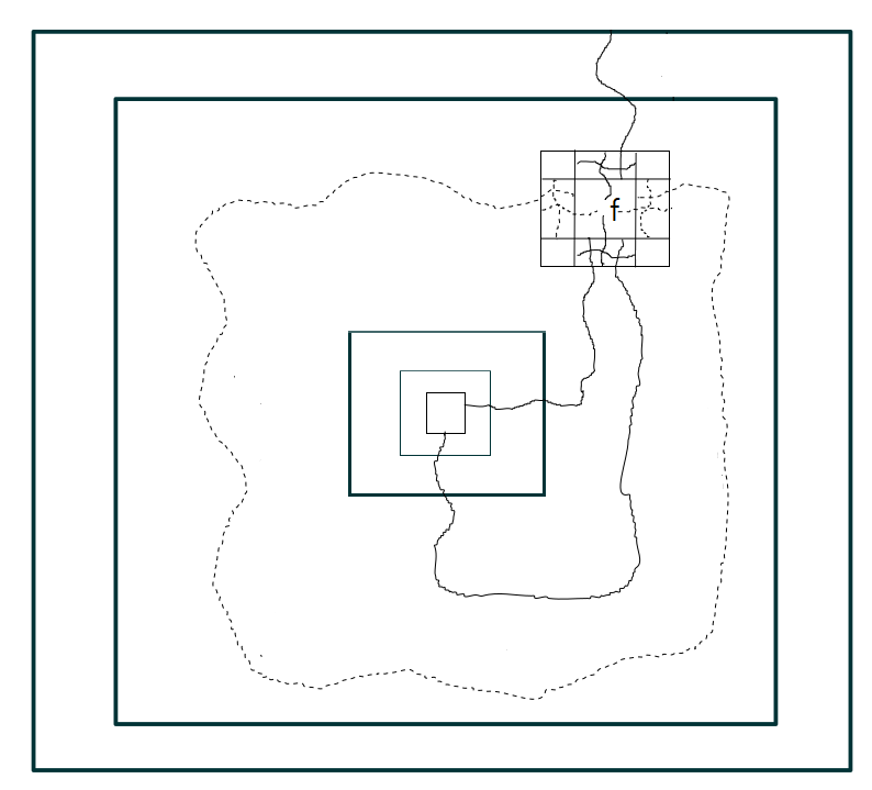
Figure 4: The event $\bar{D}(n)$. The boxes, in order from smallest to largest, are $B(n)$, $B(2n)$, $B(4n)$, $B(8n)$ and $B(16n)$. The solid circuit in Ann($2n,4n$) is $q_{n}$-open. The solid paths from $\partial B(n)$ to $f$ and the solid path from $f$ to $\partial B(16n)$ are $p_{c}$-open. The dotted circuit in Ann($4n,8n$) is $p_{c}$-closed.

The event described in $[b]$ guarantees item 2(a) in the definition of $D^{e}_{int}(n,\hat{D}_{\ast})$. Since the event described in $[c]$ has a $p_{c}$-open path from $\partial B(n)$ to $\partial B(16n)$ containing $f$ without using $e$, the event $[c]$ implies item 2(b) in the definition of $D^{e}_{int}(n,\hat{D}_{\ast})$. Therefore, for any circuit $\hat{D}^{e}_{\ast}\subset$ Ann($8n,16n$), we can estimate the sum in the bottom of (2.3.10):

$$\sum_{e\subset\text{Ann}(2n,4n)}\mathbb{P}\left(e\ext@arrow 9999{\arrowfill@\leftarrow\relbar\rightarrow}{}{q_{n}}\partial B(n)\text{ in }B(4n),D^{e}_{int}(n,\hat{D}_{\ast})\right)$$

$$\geq~{} \sum_{e\subset\hat{B}_{n}}\mathbb{P}\left(e\ext@arrow 9999{\arrowfill@\leftarrow\relbar\rightarrow}{}{q_{n}}\partial B(n)\text{ in }B(4n)\cap(-\infty,-n]\times\mathbb{R},\bar{D}(n)\right).$$ (2.3.11)

By applying the generalized FKG inequality (positive correlation for certain increasing and decreasing events, so long as they depend on particular regions of space — see [15, Lem. 13]) and a gluing construction, one can decouple the events described in $\bar{D}(n)$ and the event $\{e\ext@arrow 9999{\arrowfill@\leftarrow\relbar\rightarrow}{}{p_{c}}\partial B(n)$ in $B(4n)\cap(-\infty,-n]\times\mathbb{R}\}$ to obtain the lower bound for (2.3.11) of

$$\sum_{e\subset\hat{B}_{n}}\mathbb{P}(e\ext@arrow 9999{\arrowfill@\leftarrow\relbar\rightarrow}{}{q_{n}}\partial B(n)\text{ in }B(4n)\cap(-\infty,-n]\times\mathbb{R})\mathbb{P}([a])\mathbb{P}([b],[c])$$

$$\geq~{} c_{2}\mathbb{P}([b],[c])\sum_{e\subset\hat{B}_{n}}\mathbb{P}(e\ext@arrow 9999{\arrowfill@\leftarrow\relbar\rightarrow}{}{q_{n}}\partial B(n)\text{ in }B(4n)\cap(-\infty,-n]\times\mathbb{R}).$$ (2.3.12)

To give a lower bound for $\mathbb{P}([b],[c])$, let $A(n,f)$ be the event described in [b] and [c] (along with the condition $\omega(f)\in(q_{n},p_{c})$), so that this probability equals $\mathbb{P}(\cup_{f}A(n,f))$, and the union is over $f\subset\text{Ann}(6n,7n)\cap[6n,\infty)^{2}$. Letting $A^{\prime}(n,f)$ be the same event, but with the $p_{c}$-open paths from [c] replaced by $q_{n}$-open paths, we obtain

$$\mathbb{P}([b],[c])=\mathbb{P}(\cup_{f}A(n,f))\geq\mathbb{P}(\cup_{f}A^{\prime}(n,f)).$$

Note that the events $A^{\prime}(n,f)$ for distinct $f$ are disjoint. Therefore

$$\mathbb{P}([b],[c])\geq\sum_{f}\mathbb{P}(A^{\prime}(n,f)).$$ (2.3.13)

By a gluing argument involving the RSW theorem, the generalized FKG inequality, and Kesten’s arms direction method (see [12, Eq. (2.9)]), if we define $B(n,f)$ as the event that there are two disjoint $q_{n}$-open paths connecting $f$ to $\partial B(f,n)$, and two disjoint $p_{c}$-closed dual paths connecting $f^{*}$ to $\partial B(f,n)$, then by using independence of the value of $\omega(f)$ from the event $A^{\prime}(n,f)$, we can obtain

$$\mathbb{P}(A^{\prime}(n,f))\geq c_{3}(p_{c}-q_{n})\mathbb{P}(B(f,n)).$$ (2.3.14)

Last, by a variant of [5, Lemma 6.3] (instead of taking $p,q\in[p_{c},p_{n}]$, one takes $p,q\in[q_{n},p_{c}]$, with $p=q_{n}$ and $q=p_{c}$, and the proof is nearly identical), we have $\mathbb{P}(B(f,n))\asymp\mathbb{P}(A_{n}^{2,2})$, where $A_{n}^{2,2}$ is the four-arm event from (2.1.6). Using this with (2.3.13) and (2.3.14) gives

$$\mathbb{P}([b],[c])\geq c_{4}(p_{c}-q_{n})\sum_{f}\mathbb{P}(A_{n}^{2,2}).$$

By (2.1.6), we establish $\mathbb{P}([b],[c])\geq c_{5}$, and putting this in (2.3.12),

$$\sum_{e\subset\hat{B}_{n}}\mathbb{P}(e\ext@arrow 9999{\arrowfill@\leftarrow\relbar\rightarrow}{}{q_{n}}\partial B(n)\text{ in }B(4n)\cap(-\infty,-n]\times\mathbb{R})\mathbb{P}([a])\mathbb{P}([b],[c])$$

$$\geq~{} c_{2}c_{5}\sum_{e\subset\hat{B}_{n}}\mathbb{P}(e\ext@arrow 9999{\arrowfill@\leftarrow\relbar\rightarrow}{}{q_{n}}\partial B(n)\text{ in }B(4n)\cap(-\infty,-n]\times\mathbb{R}).$$ (2.3.15)

Last, to deal with the summand of (2.3.15), we can use a gluing construction along with the FKG inequality and the RSW theorem to obtain

$$\mathbb{P}(e\ext@arrow 9999{\arrowfill@\leftarrow\relbar\rightarrow}{}{q_{n}}\partial B(n))\geq c_{6}\mathbb{P}(e\ext@arrow 9999{\arrowfill@\leftarrow\relbar\rightarrow}{}{q_{n}}\partial B(e,dist(e,\partial B(n))),$$

where $dist$ is the $\ell_{\infty}$-distance. By (2.1.1) and (2.1.5), we have

$$\mathbb{P}(e\ext@arrow 9999{\arrowfill@\leftarrow\relbar\rightarrow}{}{q_{n}}\partial B(e,dist(e,\partial B(n))))\geq c_{7}\mathbb{P}(e\ext@arrow 9999{\arrowfill@\leftarrow\relbar\rightarrow}{}{p_{c}}\partial B(e,dist(e,\partial B(n))))\geq c_{8}\pi(n).$$

Placing this in (2.3.15) and summing over $e$ finally gives

$$\sum_{e\subset\text{Ann}(2n,4n)}\mathbb{P}\left(\omega(e)>p_{c},e\ext@arrow 9999{\arrowfill@\leftarrow\relbar\rightarrow}{}{q_{n}}\partial B(n)\text{ in }B(4n),D^{e}_{int}(n,\hat{D}_{\ast})\right)\geq c_{9}n^{2}\pi(n),$$

which finishes the proof of (2.3.8).

∎

Applying the lemma to the lower bound from (2.3.7), we obtain for all $C\geq\mathcal{C}_{6}$

$${\mathbb{E}}\Xi_{t_{n}}(\epsilon) \geq\frac{\epsilon}{1-p_{c}}C_{21}n^{2}\pi(n)\sum_{\hat{D}_{\ast}}\mathbb{P}(D^{e}_{ext}(n,\hat{D}_{\ast}),Z(\hat{D}_{\ast})>Cn^{2}\pi(n))$$

$$=\frac{\epsilon}{1-p_{c}}C_{21}n^{2}\pi(n)\mathbb{P}\left(\bigcup_{\hat{D}_{\ast}}\{D^{e}_{ext}(n,\hat{D}_{\ast}),Z(\hat{D}_{\ast})>Cn^{2}\pi(n)\}\right)$$

$$\geq\frac{\epsilon}{1-p_{c}}C_{21}n^{2}\pi(n)\mathbb{P}(A_{n},B_{n}(C)),$$

where $A_{n}$ is the event that there is a $p_{c}$-open circuit around the origin in Ann$(8n,16n)$ and $B_{n}(C)$ is the event that there are more than $Cn^{2}\pi(n)$ vertices in $B(16n)^{c}$ connected to $B(16n)$ by $p_{c}$-open paths. By the FKG inequality and the RSW theorem,

$${\mathbb{E}}\Xi_{t_{n}}(\epsilon)\geq\frac{\epsilon}{1-p_{c}}C_{21}C_{22}n^{2}\pi(n)\mathbb{P}(B_{n}(C))\text{ for $n\geq 1$, all $\epsilon>0$, and $C\geq\mathcal{C}_{6}$}.$$ (2.3.16)

Last, we argue that there exists a function $F$ on $[0,\infty)$ such that $\inf_{r\in[0,m]}F(r)>0$ for each $m\geq 0$ and such that

$$\mathbb{P}(B_{n}(C))\geq F(C)\text{ for all }n\geq 1\text{ and }C\geq 0.$$ (2.3.17)

Combining this with (2.3.16) and setting $G(C)=C_{21}C_{22}F(C)/(1-p_{c})$ will complete the proof of Proposition 2.1 and therefore of the proof of the upper bound in Theorem 1.1.

To show (2.3.17), we use some standard percolation arguments. For $\ell\geq 5$, set

$$Z_{n}(\ell):=\#\{v\in\text{Ann}(2^{\ell}n,2^{\ell+1}n):v\ext@arrow 9999{\arrowfill@\leftarrow\relbar\rightarrow}{}{\;p_{c}\;}\partial B(16n)\}.$$

By definition of $Z_{n}(\ell)$ and $B_{n}(C)$,

$$\mathbb{P}(B_{n}(C))\geq\mathbb{P}(Z_{n}(\ell)>Cn^{2}\pi(n))\text{ for any }\ell\geq 5.$$ (2.3.18)

To give a lower bound for the probability of $Z_{n}(\ell)$, we use the second moment method (Paley-Zygmund inequality):

$$\mathbb{P}\left(Z_{n}(\ell)\geq\frac{1}{2}{\mathbb{E}}Z_{n}(\ell)\right)\geq\frac{1}{4}\frac{({\mathbb{E}}Z_{n}(\ell))^{2}}{{\mathbb{E}}Z_{n}(\ell)^{2}}.$$ (2.3.19)

Accordingly, we need a lower bound for ${\mathbb{E}}Z_{n}(\ell)$ and an upper bound for ${\mathbb{E}}Z_{n}(\ell)^{2}$.

To bound ${\mathbb{E}}Z_{n}(\ell)$ from below, note that if there is a $p_{c}$-open circuit around the origin in $\text{Ann}(2^{\ell+1}n,2^{\ell+2}n)$ and a $p_{c}$-open path connecting $B(16n)$ to $\partial B(2^{\ell+2}n)$, then any point $v\in\text{Ann}(2^{\ell}n,2^{\ell+1}n)$ that is connected by a $p_{c}$-open path to $\partial B(v,2^{\ell+3})$ (the box of sidelength $2\cdot 2^{\ell+3}$ centered at $v$) contributes to $Z_{n}(\ell)$. By the FKG inequality and the RSW theorem, then,

$${\mathbb{E}}Z_{n}(\ell)\geq c_{10}f(\ell)\pi(2^{\ell+3}n)\#\{v:v\in\text{Ann}(2^{\ell}n,2^{\ell+1}n)\}.$$

Here, $c_{10}$ is a lower bound for the probability of existence of the circuit, $f(\ell)>0$ is a lower bound (depending only on $\ell$) for the probability of a connection between the two boxes, and $\pi(2^{\ell+3}n)$ is the probability corresponding to the connection between $v$ and $\partial B(v,2^{\ell+3}n)$. By (2.1.5), we obtain

$${\mathbb{E}}Z_{n}(\ell)\geq\left[c_{10}\frac{D_{1}}{\sqrt{2^{\ell+3}}}2^{2\ell}\right]n^{2}\pi(n).$$

If we fix $\ell=\ell_{0}$ so large that this is bigger than $2Cn^{2}\pi(n)$ for all $n$, we obtain from (2.3.18) and (2.3.19) that

$$\mathbb{P}(B_{n}(C))\geq\frac{C^{2}(n^{2}\pi(n))^{2}}{{\mathbb{E}}Z_{n}(\ell_{0})^{2}}.$$ (2.3.20)

For the upper bound on ${\mathbb{E}}Z_{n}(\ell_{0})^{2}$, we follow the strategy of Kesten in [11, p. 388-391]. First note that any $v$ counted in $Z_{n}(\ell_{0})$ must have a $p_{c}$-open path connecting it to $\partial B(v,2^{\ell_{0}-1}n)$. Therefore by independence,

$${\mathbb{E}}Z_{n}(\ell_{0})^{2} \leq\sum_{v,w\in\text{Ann}(2^{\ell_{0}}n,2^{\ell_{0}+1}n)}\mathbb{P}(v\ext@arrow 9999{\arrowfill@\leftarrow\relbar\rightarrow}{}{p_{c}}\partial B(v,2^{\ell_{0}-1}n),w\ext@arrow 9999{\arrowfill@\leftarrow\relbar\rightarrow}{}{p_{c}}\partial B(w,2^{\ell_{0}-1}n))$$

$$\leq\sum_{v\in\text{Ann}(2^{\ell_{0}}n,2^{\ell_{0}+1}n)}\sum_{k=0}^{2^{\ell_{0}+2}n}\sum_{w:\|v-w\|_{\infty}=k}\pi(k/2)\pi(k/2)\pi(2k,2^{\ell_{0}-1}n).$$ (2.3.21)

Here, $\pi(2k,2^{\ell_{0}-1}n)$ is the probability that there is an open path connecting $B(2k)$ to $\partial B(2^{\ell_{0}-1}n)$. (If $2k\geq 2^{\ell_{0}-1}n$, this probability is one.) By quasimultiplicativity [15, Eq. (4.17)] and the RSW theorem, we have

$$\pi(k/2)\pi(2k,2^{\ell_{0}}n)\leq C_{23}\pi(2^{\ell_{0}}n),$$

which is itself bounded by $C_{23}\pi(n)$, so putting this in (2.3.21), we have an upper bound

$${\mathbb{E}}Z_{n}(\ell_{0})^{2}\leq\left[C_{23}2^{2\ell_{0}}\sum_{k=0}^{2^{\ell_{0}+2}n}\pi(k)\right]n^{2}\pi(n).$$

By [11, Eq. (7)], we have $\sum_{k=0}^{2^{\ell_{0}+2}n}\pi(k)\leq C_{24}2^{2(\ell_{0}+2)}n^{2}\pi(n)$, and so we finish with ${\mathbb{E}}Z_{n}(\ell_{0})^{2}\leq C_{25}(n^{2}\pi(n))^{2}$, where $C_{25}$ depends only on $\ell_{0}$. Putting this into (2.3.20) finishes the proof of (2.3.17). ∎

Acknowledgements The research of M.D. is supported by an NSF CAREER grant.

References

- [1] R. Chandler, J. Koplik, K. Lerman, and J. F. Willemsen, Capillary displacement and percolation in porous media, Journal of Fluid Mechanics 119 (1982), 249–267.
- [2] J. T. Chayes, L. Chayes, and C. M. Newman, The stochastic geometry of invasion percolation, Comm. Math. Phys. 101 (1985), no. 3, 383–407. MR 815191
- [3] Michael Damron and Artëm Sapozhnikov, Outlets of 2D invasion percolation and multiple-armed incipient infinite clusters, Probab. Theory Related Fields 150 (2011), no. 1-2, 257–294. MR 2800910
- [4] Michael Damron and Artëm Sapozhnikov, Limit theorems for 2D invasion percolation, Ann. Probab. 40 (2012), no. 3, 893–920. MR 2962082
- [5] Michael Damron, Artëm Sapozhnikov, and Bálint Vágvölgyi, Relations between invasion percolation and critical percolation in two dimensions, Ann. Probab. 37 (2009), no. 6, 2297–2331. MR 2573559
- [6] Christophe Garban, Gábor Pete, and Oded Schramm, The scaling limits of the minimal spanning tree and invasion percolation in the plane, Ann. Probab. 46 (2018), no. 6, 3501–3557. MR 3857861
- [7] G. R. Grimmett and J. M. Marstrand, The supercritical phase of percolation is well behaved, Proc. Roy. Soc. London Ser. A 430 (1990), no. 1879, 439–457. MR 1068308
- [8] Geoffrey Grimmett, Percolation, Springer-Verlag, New York, 1989. MR 995460
- [9] T. E. Harris, A lower bound for the critical probability in a certain percolation process, Proc. Cambridge Philos. Soc. 56 (1960), 13–20. MR 0115221
- [10] Antal A. Járai, Invasion percolation and the incipient infinite cluster in 2D, Comm. Math. Phys. 236 (2003), no. 2, 311–334. MR 1981994
- [11] Harry Kesten, The incipient infinite cluster in two-dimensional percolation, Probab. Theory Related Fields 73 (1986), no. 3, 369–394. MR 859839
- [12] , Scaling relations for D-percolation, Comm. Math. Phys. 109 (1987), no. 1, 109–156. MR 879034
- [13] R Lenormand and S Bories, Description d’un mecanisme de connexion de liaision destine a l’etude du drainage avec piegeage en milieu poreux, CR Acad. Sci 291 (1980), 279–282.
- [14] M. V. Men’shikov and A. F. Sidorenko, Coincidence of critical points in Poisson percolation models, Teor. Veroyatnost. i Primenen. 32 (1987), no. 3, 603–606. MR 914958
- [15] Pierre Nolin, Near-critical percolation in two dimensions, Electron. J. Probab. 13 (2008), no. 55, 1562–1623. MR 2438816
- [16] J. van den Berg and H. Kesten, Inequalities with applications to percolation and reliability, J. Appl. Probab. 22 (1985), no. 3, 556–569. MR 799280
- [17] D Wilkinson and M Barsony, Monte carlo study of invasion percolation clusters in two and three dimensions, Journal of Physics A: Mathematical and General 17 (1984), no. 3, L129–L135.
- [18] David Wilkinson and Jorge F. Willemsen, Invasion percolation: a new form of percolation theory, J. Phys. A 16 (1983), no. 14, 3365–3376. MR 725616
- [19] Yu Zhang, The fractal volume of the two-dimensional invasion percolation cluster, Comm. Math. Phys. 167 (1995), no. 2, 237–254. MR 1316507