Nonlinear flavor development of a two-dimensional neutrino gas

Abstract

We present a numerical survey of the nonlinear flavor development of dense neutrino gases. This study is based on the stationary, two-dimensional ($x$ and $z$), two-beam, monochromatic neutrino line model with a periodic boundary condition along the $x$ direction. Similar to a previous work, we find that small-scale flavor structures can develop in a neutrino gas even if the physical conditions are nearly homogeneous along the $x$ axis initially. The power diffusion from the large-scale to small-scale structures increases with the neutrino density and helps to establish a semi-exponential dependence of the magnitudes of the Fourier moments on the corresponding wave numbers. The overall flavor conversion probabilities in the neutrino gases with small initial sinusoidal perturbations reach certain equilibrium values at large distances which are mainly determined by the neutrino-antineutrino asymmetry. Similar phenomena also exist in a neutrino gas with a localized initial perturbation, albeit only inside an expanding flavor conversion region. Our work suggests that a statistical treatment may be possible for the collective flavor oscillations of a dense neutrino gas in a multi-dimensional environment.

I Introduction

Due to the mismatch between its weak-interaction and vacuum (mass) states, a neutrino can experience flavor transformation or oscillations even in vacuum (see, e.g., Ref. Tanabashi et al. (2018) for a review). In the limit of coherent forward scattering (i.e., with no momentum exchange), a neutrino can experience a flavor dependent refraction in matter through the scattering by the charged leptons and nucleons in ordinary matter Wolfenstein (1978); Mikheyev and Smirnov (1985). Similarly, the neutrinos in a dense neutrino medium can also experience flavor dependent refraction through the neutrino-neutrino scattering Fuller et al. (1987); Notzold and Raffelt (1988); Pantaleone (1992). Unlike in ordinary matter, however, the so-called neutrino self-coupling potential can result in a feature-rich, collective flavor transformation which is coherent among different momentum modes of the neutrino medium (see, e.g., Ref. Duan et al. (2010) for a review).

It is beyond the current means to solve the dynamic flavor evolution in an dense, anistropic, inhomogeneous neutrino medium. Instead, simplified models were studied with certain spatial and directional symmetries imposed. For example, the isotropic and homogeneous neutrino gas model has been employed to study the neutrino oscillations in the early universe (e.g., Kostelecky et al. (1993); Abazajian et al. (2002)), and the stationary, spherical neutrino bulb model was used to study the neutrino flavor transformation in supernovae (e.g., Duan et al. (2006a, b)). The studies of these restricted models have brought many valuable insights into this intriguing quantum phenomenon including the flavor pendulum model Hannestad et al. (2006) and the analytical understanding of the spectral swaps/splits Raffelt and Smirnov (2007).

The real physical environments such as that inside a core-collapse supernova, however, can be highly anistropic and inhomogeneous. Even if certain directional and spatial symmetries are approximately held in a neutrino medium, they can be broken spontaneously during the collective flavor transformation Raffelt et al. (2013); Mirizzi (2013); Duan (2013); Mangano et al. (2014); Duan and Shalgar (2015); Chakraborty et al. (2016a); Mirizzi et al. (2015); Mirizzi (2015); Capozzi et al. (2016) (see also Ref. Duan (2015) for a review). Consider, for example, the two-dimensional (2D) neutrino line model in which the neutrinos are emitted from the “neutrino line” along the $x$ axis and propagate in the $x$-$z$ plane. After linearizing the equation of motion one can show Duan and Shalgar (2015) that the amplitudes of the inhomogeneous oscillation modes (whose flavor compositions vary along the $x$ axis) can grow exponentially as functions of $z$ in the linear regime. Unlike the restricted models, it is numerically challenging to solve the neutrino oscillations without the spatial symmetries. As a result, there have been only a few published works devoted to this subject with very limited results Mangano et al. (2014); Mirizzi et al. (2015); Mirizzi (2015).

In this work we presented a numerical survey on the inhomogeneous, nonlinear flavor transformation of dense neutrino gases. This study is based on the simplest 2D neutrino line model with two beams of monochromatic neutrinos and antineutrinos emitted from each point along the neutrino line. Through this work we wish to stimulate the interest of developing an analytic understanding of the nonlinear flavor transformation in the simplest 2D model which may bring further insights into the more realistic models. To keep the problem simple, we will ignore the temporal instabilities Abbar and Duan (2015); Dasgupta and Mirizzi (2015), fast flavor conversions Sawyer (2016); Chakraborty et al. (2016b), the collisional effects Cirigliano et al. (2017); Capozzi et al. (2018), and many other recent developments (see Ref. Chakraborty et al. (2016c) for a review).

The rest of the paper is organized as follows. In Sec. II we will describe the two-beam, neutrino line model in detail and review the current analytic understanding of this model. In Sec. III we will briefly describe the numerical method we used to solve the line model and present a survey of the nonlinear flavor transformation of the neutrino gas in this model with various physical parameter choices. In Sec. IV we give our conclusions.

II The neutrino line model

In this section we first establish the formalism by explaining the neutrino line model proposed in Ref. Duan and Shalgar (2015). We then briefly review the flavor pendulum model Hannestad et al. (2006) which describes the flavor evolution in the neutrino line model when both the spatial and directional symmetries are preserved. We will also briefly review the linearized flavor stability analysis performed in Ref. Duan and Shalgar (2015) which describes the flavor evolution in the linear regime.

II.1 Equations of motion

We study the mixing between two (effective) neutrino flavors $\nu_{e}$ and $\nu_{\tau}$, with $\nu_{\tau}$ being a suitable linear combination of the physical $\nu_{\mu}$ and $\nu_{\tau}$. We use the (flavor) polarization vector $\mathbf{P}_{\vec{p}}(t,{\vec{r}})$ in flavor space to represent the flavor quantum state of a neutrino of momentum ${\vec{p}}$ at time $t$ and position ${\vec{r}}$. We define the unit (flavor) basis vectors $\mathbf{e}_{i}$ ($i=1,2,3$) such that $P_{3}=\mathbf{P}\cdot\mathbf{e}_{3}$ gives the probability $\mathcal{P}_{\nu_{e}}$ of the neutrino being in the electron flavor through the relation

$$\mathcal{P}_{\nu_{e}}=\frac{1}{2}(1+P_{3}),$$ (1)

and $P_{1}$ and $P_{2}$ describe the coherence between the two flavors. The polarization vector $\bar{\mathbf{P}}$ for the antineutrino is defined in a similar way.

In absence of neutrino emission, absorption, and collision, the polarization vectors obey the following equations of motion Sigl and Raffelt (1993)

$$(\partial_{t}+{\hat{v}}\cdot\overrightarrow{\nabla})\mathbf{P}_{{\vec{p}}} =(\omega\mathbf{B}+\lambda\mathbf{e}_{3}+\mathbf{V}_{{\vec{p}}})\times\mathbf{P}_{{\vec{p}}},$$ (2a)

$$(\partial_{t}+{\hat{v}}\cdot\overrightarrow{\nabla})\bar{\mathbf{P}}_{{\vec{p}}} =(-\omega\mathbf{B}+\lambda\mathbf{e}_{3}+\mathbf{V}_{{\vec{p}}})\times\bar{\mathbf{P}}_{{\vec{p}}}.$$ (2b)

In the above equation, ${\hat{v}}={\vec{p}}/|{\vec{p}}|$ and $\omega=\delta m^{2}/2|{\vec{p}}|$ are the velocity and vacuum oscillation frequency of the neutrino, respectively, $\mathbf{B}=\sin(2\theta_{\text{v}})\mathbf{e}_{1}-\cos(2\theta_{\text{v}})\mathbf{e}_{3}$ is a unit vector that denotes the neutrino mixing in vacuum, $\lambda=\sqrt{2}G_{\text{F}}n_{e}$ is the matter potential with $G_{\text{F}}$ being the Fermi coupling constant and $n_{e}$ the net electron number density, and

$$\mathbf{V}_{\vec{p}}=\sqrt{2}G_{\text{F}}\int\!\frac{{\text{d}}^{3}p^{\prime}}{(2\pi)^{3}}(1-{\hat{v}}\cdot{\hat{v}}^{\prime})\{[f_{\nu_{e}}({\vec{p}}^{\prime})-f_{\nu_{\tau}}({\vec{p}}^{\prime})]\mathbf{P}_{{\vec{p}}^{\prime}}-[f_{\bar{\nu}_{e}}({\vec{p}}^{\prime})-f_{\bar{\nu}_{\tau}}({\vec{p}}^{\prime})]\bar{\mathbf{P}}_{{\vec{p}}^{\prime}}\},$$ (3)

is the neutrino self-coupling potential with $f_{\nu}({\vec{p}})$ ($\nu=\nu_{e}$, $\nu_{\tau}$, $\bar{\nu}_{e}$ and $\bar{\nu}_{\tau}$) being the initial occupation numbers of the neutrinos of momentum ${\vec{p}}$ in the corresponding flavor states.

We adopt the convention that the neutrino mass-squared difference $\delta m^{2}$ is always positive and that the normal and inverted neutrino mass hierarchies (NH and IH) are represented by the vacuum mixing angles $\theta_{\text{v}}$ within the ranges of $(0,\pi/4)$ and $(\pi/4,\pi/2)$, respectively.

We restrict our study to the two-beam, monchromatic neutrino line model in which mono-energetic $\nu_{e}$’s and $\bar{\nu}_{e}$’s are constantly emitted in two directions, ${\hat{v}}_{\pm}=(\pm u,0,v_{z})$, from each point on the $x$ axis, where $u=\sqrt{1-v_{z}^{2}}$. In this model, the convection operator becomes

$$\partial_{t}+{\hat{v}}\cdot\overrightarrow{\nabla}\longrightarrow D_{\pm}=\pm u\partial_{x}+v_{z}\partial_{z}.$$ (4)

Because the presence of a large matter density does not suppress collective oscillations in this model other than reducing the effective neutrino mixing angle Duan et al. (2006c); Hannestad et al. (2006), we will work in the appropriate frame rotating about $\mathbf{e}_{3}$ in flavor space in which

$$\pm\omega\mathbf{B}+\lambda\mathbf{e}_{3}\xrightarrow{\lambda\gg\omega}\mp\eta\,\omega_{\text{eff}}\,\mathbf{e}_{3},$$ (5)

where $\eta=\text{sgn}(\cos 2\theta_{\text{v}})$ is the signature of the neutrino mass hierarchy, and

$$\omega_{\text{eff}}=\omega\,|\cos 2\theta_{\text{v}}|$$ (6)

is the effective oscillation frequency of the neutrino. In the rest of the paper, we will measure the energies in terms of $\omega_{\text{eff}}$ by setting

$$\omega_{\text{eff}}=1.$$ (7)

Equation (2) now reduces to

$$D_{\pm}\mathbf{P}_{\pm} =[-\eta\mathbf{e}_{3}+\mu(\mathbf{P}_{\mp}-\alpha\bar{\mathbf{P}}_{\mp})]\times\mathbf{P}_{\pm},$$ (8a)

$$D_{\pm}\bar{\mathbf{P}}_{\pm} =[+\eta\mathbf{e}_{3}+\mu(\mathbf{P}_{\mp}-\alpha\bar{\mathbf{P}}_{\mp})]\times\bar{\mathbf{P}}_{\pm},$$ (8b)

where the subscripts “$\pm$” denote the right- and left-going neutrino beams, respectively. In Eq. (8), the parameters

$$\mu=2\sqrt{2}G_{\text{F}}n_{\nu_{e}}(1-v_{z}^{2})$$ (9)

and

$$\alpha=\frac{n_{\bar{\nu}_{e}}}{n_{\nu_{e}}}$$ (10)

measures the strength of the neutrino potential and the neutrino-antineutrino asymmetry, respectively, where $n_{\nu_{e}}$ and $n_{\bar{\nu}_{e}}$ are the number densities of the corresponding neutrino species. We assume that both $\mu$ and $\alpha$ are constant in the whole space.

From Eq. (8) it is easy to show that the average electron lepton number

$$\mathcal{L}=\frac{1}{4L}\int_{0}^{L}[(2+P_{3+}+P_{3-})-\alpha(2+\bar{P}_{3+}+\bar{P}_{3-})]\,{\text{d}}x$$ (11)

is constant along $z$.

II.2 The flavor pendulum

If the neutrino emission is homogeneous along the $x$ axis and symmetric between the two directions, then

$$\mathbf{P}_{\pm}(x,z)\longrightarrow\mathbf{P}(z)\quad\text{and}\quad\bar{\mathbf{P}}_{\pm}(x,z)\longrightarrow\bar{\mathbf{P}}(z).$$ (12)

In this limit, the two-beam neutrino line model reduces to the bipolar model Kostelecky and Samuel (1995); Duan et al. (2006c), and its flavor evolution is equivalent to the motion of a pendulum in flavor space with a total angular momentum $\mathbf{D}=\mathbf{P}-\alpha\bar{\mathbf{P}}$ Hannestad et al. (2006). Defining $\mathbf{Q}=\mathbf{P}+\alpha\bar{\mathbf{P}}+\eta\mathbf{e}_{3}/\mu$ and using Eq. (8) one can show that

$$\dot{\mathbf{D}}=\mathbf{q}\times(\eta|\mathbf{Q}|)\mathbf{e}_{3},$$ (13)

where $\dot{F}(z)=v_{z}{\text{d}}F/{\text{d}}z$ for an arbitrary function $F(z)$, and $\mathbf{q}=\mathbf{Q}/|\mathbf{Q}|$ and $(\eta|\mathbf{Q}|)\mathbf{e}_{3}$ are the “position” and “weight” of the pendulum bob, respectively. The spin $\sigma=\mathbf{D}\cdot\mathbf{q}$ of the bob is conserved, and

$$\frac{1}{\mu}\mathbf{q}\times\dot{\mathbf{q}}=\mathbf{D}-\sigma\mathbf{q}$$ (14)

is the orbital angular momentum of the bob.

The pendulum model has been used to obtain many useful insights of the flavor evolution of the bipolar model Hannestad et al. (2006); Duan et al. (2007). For example, one can easily see that no (significant) flavor transformation can occur at $\mu\gg 1$ if the neutrino mass hierarchy is normal ($\eta=+1$) because the flavor pendulum is near its stable configuration initially. If $\eta=-1$ (IH), flavor oscillation will occur only if

$$\frac{2}{(1+\sqrt{\alpha})^{2}}<\mu<\frac{2}{(1-\sqrt{\alpha})^{2}},$$ (15)

and $P_{3}$ has a minimum value

$$P_{3,\text{min}}=-\alpha+\frac{1}{4}\mu(1-\alpha)^{2}+\frac{1}{\mu}.$$ (16)

No significant flavor oscillation occurs if $\mu>2/(1-\sqrt{\alpha})^{2}$ where the flavor pendulum behaves like a sleeping top Duan et al. (2007).

II.3 Spontaneous symmetry breaking

It turns out that an initially homogeneous neutrino gas can lose its homogeneity during collective oscillations Duan and Shalgar (2015); Mirizzi et al. (2015). To see this, we assume the following periodic boundary conditions along the $x$ axis:

$$\mathbf{P}_{\pm}(0,z)=\mathbf{P}_{\pm}(L,z)\quad\text{and}\quad\bar{\mathbf{P}}_{\pm}(0,z)=\bar{\mathbf{P}}_{\pm}(L,z)$$ (17)

as in Refs. Duan and Shalgar (2015); Mirizzi et al. (2015), where $L$ is the size of the periodic box. Performing the Fourier transformation along the $x$ axis one obtains

$$\mathbf{P}^{(m)}_{\pm}(z)=\frac{1}{L}\int_{0}^{L}e^{-{\text{i}}k_{m}x}\mathbf{P}_{\pm}(x,z)\,{\text{d}}x$$ (18)

and a similar expression for $\bar{\mathbf{P}}^{(m)}_{\pm}(z)$, where $k_{m}=2m\pi/L$ ($m=0,\pm 1,\cdots$). Eq. (8) now becomes

$$\dot{\mathbf{P}}^{(m)}_{\pm} =\mp{\text{i}}k_{m}u\mathbf{P}^{(m)}_{\pm}-\eta\mathbf{e}_{3}\times\mathbf{P}^{(m)}_{\pm}+\mu\sum_{m^{\prime}}[\mathbf{P}^{(m^{\prime})}_{\mp}-\alpha\bar{\mathbf{P}}^{(m^{\prime})}_{\mp}]\times\mathbf{P}^{(m-m^{\prime})}_{\pm}$$ (19a)

$$\dot{\bar{\mathbf{P}}}^{(m)}_{\pm} =\mp{\text{i}}k_{m}u\bar{\mathbf{P}}^{(m)}_{\pm}+\eta\mathbf{e}_{3}\times\bar{\mathbf{P}}^{(m)}_{\pm}+\mu\sum_{m^{\prime}}[\mathbf{P}^{(m^{\prime})}_{\mp}-\alpha\bar{\mathbf{P}}^{(m^{\prime})}_{\mp}]\times\bar{\mathbf{P}}^{(m-m^{\prime})}_{\pm}.$$ (19b)

Because of the coupling among the different Fourier moments, the “power” in the low Fourier moments with small wave numbers $k_{m}$ can dissipate into high moments and result in fine structures and the loss of large-scale, coherent flavor evolution. Before the translation symmetry is badly broken, however, the Fourier moments of different wave numbers evolve independently. This can be seen through the flavor stability analysis performed in Ref. Duan and Shalgar (2015) which is recapped below.

In the linear regime where the neutrino coherence fields

$$S^{(m)}_{\pm} =\mathbf{P}^{(m)}_{\pm}\cdot(\mathbf{e}_{1}-{\text{i}}\mathbf{e}_{2}),$$ (20a)

$$\bar{S}^{(m)}_{\pm} =\bar{\mathbf{P}}^{(m)}_{\pm}\cdot(\mathbf{e}_{1}-{\text{i}}\mathbf{e}_{2})$$ (20b)

are small, they obey the linearized equations of motion:

$${\text{i}}\dot{S}^{(m)}_{\pm} =[-\eta\pm uk_{m}+(1-\alpha)\mu]S^{(m)}_{\pm}$$

$$\quad-\mu[S^{(m)}_{\mp}-\alpha\bar{S}^{(m)}_{\mp}],$$ (21a)

$${\text{i}}\dot{\bar{S}}^{(m)}_{\pm} =[+\eta\pm uk_{m}+(1-\alpha)\mu]\bar{S}^{(m)}_{\pm}$$

$$\quad-\mu[S^{(m)}_{\mp}-\alpha\bar{S}^{(m)}_{\mp}].$$ (21b)

The solution to the above equation is a linear superposition of the normal modes:

$$\begin{bmatrix}S^{(m)}_{+}(z)\\ \bar{S}^{(m)}_{+}(z)\\ S^{(m)}_{-}(z)\\ \bar{S}^{(m)}_{-}(z)\end{bmatrix}=\sum_{a=1}^{4}\mathsf{S}^{(m)}_{a}e^{{\text{i}}K^{(m)}_{a}z},$$ (22)

where $\mathsf{S}^{(m)}_{a}$ and $K^{(m)}_{a}$ are the amplitudes and wave numbers of the $a$th normal mode, respectively. If there exist normal modes with $\text{Im}[K^{(m)}_{a}]>0$, the corresponding Fourier moments are unstable against the flavor conversion, and their amplitudes grow exponentially with $z$. In this case, even if there is an approximate translation symmetry along the $x$ direction, this symmetry is spontaneously broken when $|S^{(m\neq 0)}|$ and $|\bar{S}^{(m\neq 0)}|$ grow to of $\mathcal{O}(1)$.

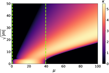
Figure 1: (Color online) The largest exponential growth rate $\kappa(m)=\text{max}(\text{Im}[K^{(m)}_{a}])$ of the flavor coherence amplitude as a function of the neutrino potential strength $\mu$ and the Fourier moment index $m$ in a two-beam neutrino line model with the neutrino-antineutrino asymetry $\alpha=0.6$ and the neutrino velocity $v_{z}=1/\sqrt{2}$ along the $z$ direction. The vertical dashed lines mark the boundaries of $\mu$ within which the homogeneous, bipolar model experiences a flavor oscillation like a flavor pendulum. This oscillation is suppressed at larger $\mu$ where the flavor pendulum behaves like a sleeping top.

In Fig. 1, we demonstrate the largest exponential growth rate $\kappa(m)=\text{max}(\text{Im}[K^{(m)}_{a}])$ of the flavor coherence amplitude as a function of both the strength of the neutrino potential $\mu$ and the Fourier index $m$ for the two-beam neutrino line with $\alpha=0.6$ and $v_{z}=1/\sqrt{2}$. We also marked the boundaries of the regime where a homogeneous neutrino gas is unstable against flavor conversion [Eq. (15)].

III Numerical Results

Following the pilot study in Ref. Mirizzi et al. (2015) which features a single parameter set ($\eta=+1$, $\alpha\approx 0.77$, and $\mu=13$), we have conducted a numerical survey of the two-beam neutrino line model for a wide range of the parameter space.We present a representative collection of our numerical results in this section. All the calculations assume the initial conditions of the following form

$$\mathbf{P}_{\pm}(x,0)=\bar{\mathbf{P}}_{\pm}(x,0) \approx[\epsilon_{\pm},0,1],$$ (23)

where $|\epsilon_{\pm}(x)|\ll 1$. We choose the emission angles of both the left- and right-going beams to be $\pi/4$. A change to the neutrino emission angle is equivalent to a change of the neutrino density and a rescaling of the $x$ and $z$ axes simultaneously. We use a relatively large box with $L=30$ compared to $L\approx 6.2$ in Ref. Mirizzi et al. (2015).

$\begin{array}[]{@{}l@{\hspace{0.01in}}l@{\hspace{0.01in}}l@{}}\includegraphics*[scale={0.3}]{fig2a.pdf}\hfil\hskip 0.72229pt&\includegraphics*[scale={0.3}]{fig2b.pdf}\hfil\hskip 0.72229pt&\includegraphics*[scale={0.3}]{fig2c.pdf}\\ \includegraphics*[scale={0.3}]{fig2d.pdf}\hfil\hskip 0.72229pt&\includegraphics*[scale={0.3}]{fig2e.pdf}\hfil\hskip 0.72229pt&\includegraphics*[scale={0.3}]{fig2f.pdf}\\ \includegraphics*[scale={0.3}]{fig2g.pdf}\hfil\hskip 0.72229pt&\includegraphics*[scale={0.3}]{fig2h.pdf}\hfil\hskip 0.72229pt&\includegraphics*[scale={0.3}]{fig2i.pdf}\end{array}$

Figure 2: (Color online) The flavor evolution of the neutrino gas in the two-beam line model with the inverted (IH, top panels) and normal (NH, middle panels) neutrino mass hierarchies, various antineutrino-to-neutrino density ratios [$\alpha=0.6$ (left), $0.7$ (middle) and $0.8$ (right)], and sinusoidal initial perturbations described in the text. All the calculations have the same density of the neutrinos which is proportional to the neutrino self-coupling strength $\mu$. The top and middle panels show the angle-averaged polarization components $\langle P_{3}\rangle$ of the neutrinos as functions of $x$ and $z$, and the bottom panels show the evolution of these components over $z$ when averaged over $x$. Also shown in the bottom panels are the values predicted by the pendulum model (dotted curves) and the equilibrium values $P^{\text{eq}}_{3}$ in the IH calculations (dot-dashed lines).

III.1 Numerical method and validation

Unlike Ref. Mirizzi et al. (2015) which solved $\mathbf{P}_{\pm}^{(m)}(z)$ and $\bar{\mathbf{P}}_{\pm}^{(m)}(z)$ from Eq. (19), we solve $\mathbf{P}_{\pm}(x,z)$ and $\bar{\mathbf{P}}_{\pm}(x,z)$ in the direct space. We discretize the $x$ axis into $N$ equal intervals and solve the equations of motion by a finite difference method derived from the Lax-Wendroff algorithm Press et al. (2002). Our code accurately recovers the pendulum-like flavor oscillation when $\epsilon_{+}=\epsilon_{-}=\text{const}$. In the linear regime where the translation symmetry along the $x$ direction is slightly broken, our code produces the correct exponential growth of the coherence amplitudes as predicted by the linearized flavor stability analysis. We varied the number of discrete bins in the $x$ direction and the error tolerance in the numerical integration along the $z$ direction to test the numerical convergence of some representative calculations. We also varied the size of the periodic box $L$ for the calculations with localized perturbations to make sure that the results are independent of the choice of $L$. We do not enforce the unitary condition, $|\mathbf{P}(x,z)|=|\bar{\mathbf{P}}(x,z)|=1$, in our code but we rather use it to check the correctness of the numerical solutions.

III.2 Sinusoidal initial perturbations

$\begin{array}[]{@{}c@{\hspace{0.5in}}c@{}}\includegraphics*[scale={0.4}]{fig3a.pdf}\hfil\hskip 36.135pt&\includegraphics*[scale={0.4}]{fig3b.pdf}\end{array}$

Figure 3: (Color online) The equilibrium values $P_{3}^{\text{eq}}$ and $\bar{P}_{3}^{\text{eq}}$ for the neutrinos (upper lines) and antineutrinos (lower lines) at large $z$ as functions of the antineutrino-to-neutrino ratio $\alpha$ (left) and as functions of the neutrino self-coupling strength $\mu$ (right), respectively. All the calculations assume the inverted neutrino mass hierarchy. The various symbols represent the calculations with $30,000$ ($\bullet$), $60,000$ ($\blacktriangle$), $120,000$ ($\blacksquare$), and $240,000$ ($\bigstar$) discrete $x$ bins, respectively. The error bars indicate the maximal and minimal values of $\langle P_{3}^{(0)}\rangle$ and $\langle\bar{P}_{3}^{(0)}\rangle$ in the distance range over which the (mean) equilibrium values are calculated. The dotted lines represent the case with $\bar{P}_{3}^{\text{eq}}=0$ where the antineutrinos are fully depolarized in flavor, and the dot-dashed lines are the corresponding values of $P_{3}^{\text{eq}}$ obtained from Eq. (27).

$\begin{array}[]{@{}l@{\hspace{0.01in}}l@{\hspace{0.01in}}l@{}}\includegraphics*[scale={0.3}]{fig4a.pdf}\hfil\hskip 0.72229pt&\includegraphics*[scale={0.3}]{fig4b.pdf}\hfil\hskip 0.72229pt&\includegraphics*[scale={0.3}]{fig4c.pdf}\\ \includegraphics*[scale={0.3}]{fig4d.pdf}\hfil\hskip 0.72229pt&\includegraphics*[scale={0.3}]{fig4e.pdf}\hfil\hskip 0.72229pt&\includegraphics*[scale={0.3}]{fig4f.pdf}\\ \includegraphics*[scale={0.3}]{fig4g.pdf}\hfil\hskip 0.72229pt&\includegraphics*[scale={0.3}]{fig4h.pdf}\hfil\hskip 0.72229pt&\includegraphics*[scale={0.3}]{fig4i.pdf}\end{array}$

Figure 4: (Color online) The development of the small-scale flavor structures in the neutrino gases with the neutrino self-coupling strengths $\mu=10$ (left panels), $25$ (middle panels) and $50$ (right panels). All the calculations assume the inverted neutrino mass hierarchy and the antineutrino-to-neutrino density ratio $\alpha=0.6$. The top panels show $\langle P_{3}\rangle$ as functions of $x$ and $z$. The lower two rows show the magnitudes of the Fourier moments of the neutrino polarization vector $|\langle\mathbf{P}^{(m)}\rangle|$ as functions of the Fourier index $m$ for a few values of $z$ (middle row), and as functions of $z$ for a few moments (bottom row). Also shown in the middle panels are the maximum exponential growth rates $\kappa$ as functions of $m$ (dashed curves with the scales on the right sides of the panels).

$\begin{array}[]{@{}l@{\hspace{0.01in}}l@{\hspace{0.01in}}l@{}}\includegraphics*[scale={0.3}]{fig5a.pdf}\hfil\hskip 0.72229pt&\includegraphics*[scale={0.3}]{fig5b.pdf}\hfil\hskip 0.72229pt&\includegraphics*[scale={0.3}]{fig5c.pdf}\\ \includegraphics*[scale={0.3}]{fig5d.pdf}\hfil\hskip 0.72229pt&\includegraphics*[scale={0.3}]{fig5e.pdf}\hfil\hskip 0.72229pt&\includegraphics*[scale={0.3}]{fig5f.pdf}\\ \includegraphics*[scale={0.3}]{fig5g.pdf}\hfil\hskip 0.72229pt&\includegraphics*[scale={0.3}]{fig5h.pdf}\hfil\hskip 0.72229pt&\includegraphics*[scale={0.3}]{fig5i.pdf}\end{array}$

Figure 5: (Color online) Similar to Fig. 2 but for highly localized initial perturbations (see text) and different values of $\alpha$ and $\mu$. In the bottom row, $\langle P_{3}\rangle_{\text{C}}$ is averaged over the central segment of the box with a width $10$. Also shown are $P_{3}^{\text{eq}}$ in the corresponding IH calculations with sinusoidal initial perturbations.

We first consider the neutrino gas with a sinusoidal initial perturbation:

$$\epsilon_{\pm}(x) =\epsilon_{0}^{\pm}+2\sum_{m>0}\epsilon_{m}^{\pm}\sin(k_{m}x),$$ (24)

where $\epsilon_{m}^{\pm}$ are constants. The results from this idealized initial condition demonstrates how the flavor evolution in the two-beam neutrino line model depends on the neutrino mass hierarchy, the neutrino-antineutrino asymmetry, and the neutrino number density.

In Fig. 2 we show $\langle P_{3}(x,z)\rangle$ with $\mu=25$ and three values of $\alpha$ for both $\eta=-1$ (IH, top panels) and $\eta=+1$ (NH, middle panels), where $\langle\cdots\rangle$ represents the average over the emission directions of the neutrino fluxes. In the bottom panels of the figure, we show the evolution of $P_{3}$ when averaged over both the neutrino emission directions and the $x$ axis.

In the IH cases, we set $\epsilon_{m}^{\pm}=0$ for all $m$ except

$$\epsilon_{0}^{\pm}=2\times 10^{-3}\quad\text{and}\quad\epsilon_{1}^{\pm}=-10^{-4}.$$ (25)

Although the left- and right-going neutrino beams have the same initial conditions at any emission point on the $x$ axis, this left-right symmetry is lost at $z>0$ when the $x$-translation symmetry is spontaneously broken. When averaged over the left- and right-going beams, however, $\langle P_{3}(x,z)\rangle$ demonstrates a residue mirror symmetry about the middle line of the box because of the left-right symmetry in the initial condition. The overall flavor evolution patterns displayed in the top panels of Fig. 2 with different values of $\alpha$ are very similar. Initially, the neutrino gas behaves like a flavor pendulum: the neutrino polarization vectors remain in their initial states for a long time before quickly swinging towards the opposite flavor states and coming back up again. The approximate $x$-translation symmetry is preserved during this pendulum-like flavor evolution until the $m=1$ mode becomes significant. After that, the large-scale flavor structures along the $x$ direction begin to break down into small-scale structures as $z$ increases. The overall flavor conversion at large $z$ increases with $\alpha$ for a fixed value of $\mu$.

The initial conditions in the NH cases shown in the middle panels of Fig. 2 are the same as in the IH cases except

$$\epsilon_{1}^{-}=2\epsilon_{1}^{+}=-2\times 10^{-4}.$$ (26)

Because the homogeneous mode is perturbed symmetrically (i.e., $\epsilon_{0}^{+}=\epsilon_{0}^{-}$) and because the flavor pendulum is stable with $\eta=+1$, the neutrino gas does not experience significant flavor conversion until the $m=1$ mode becomes significant. Similar to the IH cases, the large-scale flavor structures also break down into small-scale ones in the NH cases as $z$ increases. But compared to their IH counterparts, $\langle P_{3}(x,z)\rangle$ with the NH develop more prominent stream-like structures that are localized in the $x$ direction and extended along the $z$ direction. These stream-like flavor structures result in the “streamlines of the neutrino flux” observed in Ref. Mirizzi et al. (2015).

The results shown in the bottom panels of Fig. 2 suggest that, although the initial flavor evolution of the neutrino gas can be sensitive to the neutrino mass hierarchy and the initial condition at $z=0$, the overall flavor conversion at large $z$ appears to settle down on an equilibrium value which is almost independent of these parameters. In practice, we define $P^{\text{eq}}_{3}$ and $\bar{P}^{\text{eq}}_{3}$ to be the mean values of $\langle P_{3}^{(0)}(z)\rangle$ and $\langle\bar{P}_{3}^{(0)}(z)\rangle$ in the last distance unit of $z$ after they are saturated.

To demonstrate the dependence of $P^{\text{eq}}_{3}$ and $\bar{P}^{\text{eq}}_{3}$ on the neutrino-antineutrino asymmetry and the neutrino density, we plot $P^{\text{eq}}_{3}$ and $\bar{P}^{\text{eq}}_{3}$ in Fig. 3 in terms of $\alpha$ (left panel) and $\mu$ (right panel), respectively, both with $\eta=-1$ and the initial condition defined in Eq. (28). From Fig. 3 one can see that the antineutrinos in the two-beam line model become almost depolarized in flavor (i.e., $\bar{P}^{\text{eq}}_{3}\approx 0$) at large $z$. The depolarization is generally more complete with a larger value of $\mu$ or neutrino density. Because of the conserved electron lepton number $\mathcal{L}$ [Eq. (11)], the final mean flavor conversion of the neutrinos is related to that of the antineutrinos through

$$P^{\text{eq}}_{3}=1-\alpha(1-\bar{P}^{\text{eq}}_{3}).$$ (27)

As shown in Fig. 3, the values of $P^{\text{eq}}_{3}$ in our calculations indeed demonstrate a nearly linear dependence on $\alpha$ but little dependence on $\mu$.

Although the overall flavor conversion of the neutrino gas in the two-beam line model is largely independent of the neutrino self-coupling strength $\mu$, a larger number of $x$ bins is needed to achieve the same accuracy as $\mu$ increases (see the changing symbols in the right panel of Fig. 3). This is because more significant small-scale flavor structures are generated at smaller $z$ as $\mu$ increases. To demonstrate this interesting feature, we show the flavor evolution of the neutrino gas with the same neutrino-antineutrino asymmetry ($\alpha=0.6$) but three different values of $\mu$ in Fig. 4. All three calculations assume the inverted neutrino mass hierarchy. The initial flavor perturbations of the neutrino gas in these calculations are the same as what is defined in Eq. (28) except with

$$\epsilon_{0}^{\pm}=10^{-3},\,\epsilon_{1}^{\pm}=5\times 10^{-5}\,\text{and}\,\epsilon_{200}^{\pm}=5\times 10^{-10}$$ (28)

for the case with $\mu=50$.

Comparing the first two panels of Fig. 4 in the first row, one can clearly see that the neutrino gas with a larger value of $\mu$ or a higher neutrino density develops finer flavor structures than the one with a lower density. This fact becomes obvious when one compares the magnitudes the Fourier moments of the neutrino polarization vector $|\langle\mathbf{P}^{(m)}\rangle|$ in these two cases, as shown in the middle panels of Fig. 4. It appears that $|\langle\mathbf{P}^{(m)}\rangle|$ has a semi-exponential dependence on the Fourier index $m$ for a wide range of $m$ and $z$:

$$|\langle\mathbf{P}^{(m)}\rangle|\propto\exp[-\beta(z)\,k_{m}],$$ (29)

where the exponent $\beta(z)$ decreases with increasing $z$. The comparison between the first two panels in the second row of Fig. 4 shows that $\beta$ is smaller at the same $z$ for the neutrino gas with a larger density which indicates more prominent small-scale flavor structures.

The semi-exponential form of $|\langle\mathbf{P}^{(m)}\rangle|$ in the nonlinear regime is intriguing and cannot be explained by the linearized flavor stability analysis. In the middle panels of Fig. 4 we also plot the largest exponential growth rate $\kappa(m)$ (dashed curves) predicted by the linearized flavor stability analysis. In the first two panels of this row, one observes that the high moments rise faster than the low moments in order to maintain the semi-exponential power spectrum, while $\kappa(m)$ decreases with increasing $m$. In fact, the magnitudes of the Fourier moments with $m\gtrsim 200$ grow with $z$ for $\mu=10$ even though they are predicted to be stable in the linear regime (left panel). These results indicate that the excitation of the high moments in these calculations is not due to their own instabilities but because of the “power diffusion” from the low moments. This diffusion phenomenon is reminiscent of the development of the turbulence in an initially laminarly flowing fluid Mirizzi et al. (2015) and the kinematic decoherence in an initially isotropic neutrino gas Raffelt and Sigl (2007).

In the bottom panels of Fig. 4 we also show the evolution of the strengths of a few Fourier moments over $z$. These panels show that different Fourier moments do not reach equilibrium at the same time. The low moments are saturated first, and the high moments later. This implies that small-scale flavor structures may still develop even after the overall flavor conversion of the neutrino gas has reached its equilibrium value.

The calculations shown in the last column of Fig. 4 is special because the flavor pendulum with $\alpha=0.6$ and $\mu=50$ is in the sleeping-top regime, and the Fourier modes with $m\lesssim 50$ are stable (see Fig. 1). Therefore, we intentionally perturbed the Fourier modes with $m=\pm 200$ which exhibit the exponential growth in the linear regime (bottom panel). After these moments are excited, they couple the low moments to the high moments and, as a result, $|\langle\mathbf{P}^{(m)}\rangle|$ has semi-periodic dependence on $m$ initially (middle panel). At large $z$, however, $|\langle\mathbf{P}^{(m)}\rangle|$ in this case has a much weaker dependence on $m$ than those shown in the left two panels.

III.3 Localized perturbations

The sinusoidal initial perturbations discussed in the previous subsection are large-scale perturbations. Next we consider localized initial perturbations of the form

$$\epsilon_{\pm}(x)=\frac{\epsilon_{\text{g}}^{\pm}}{\sqrt{2\pi\sigma^{2}}}\,\exp\left[-\frac{(x-x_{0})^{2}}{2\sigma^{2}}\right],$$ (30)

where $\epsilon_{\text{g}}^{\pm}$, $x_{0}$, and $\sigma$ are constants. In Fig. 5 we show the flavor evolution of the neutrino gases with various values of $\alpha$ and $\mu$ for both the inverted (IH, top panels) and normal (NH, middle panels) neutrino mass hierarchies. For the initial perturbations, we take

$$\epsilon_{\text{g}}^{\pm} =2\times 10^{-3}, x_{0} =L/2, \sigma^{2} =0.2$$ (31)

for the IH cases, and the same initial perturbations except with

$$\epsilon_{\text{g}}^{-}=2\epsilon_{\text{g}}^{+}=4\times 10^{-3}$$ (32)

for the NH cases.

The upper two rows of Fig. 5 show that, for an initial perturbation localized around $x_{0}$, the flavor conversion first appears near $x_{0}$ and spreads out to the left and right. At large $z$ the edges of the “envelope” of the flavor conversion region are parallel to the propagation directions of the two velocity modes of the neutrinos. The flavor conversion is coherent in space near these edges, but small-scale flavor structures develop deep inside the envelope. The flavor development inside the envelope shown in Fig. 5 is qualitatively the same as that shown in Figs. 2 and 4. A larger neutrino self-coupling strength or density induces finer flavor structures, and a smaller neutrino-antineutrino asymmetry produces a larger overall flavor conversion.

We intentionally limit our calculations to $z<L/2$ to avoid the unphysical consequences because of the artificial, periodic boundary condition. As a result, the flavor evolution of the neutrino gases with localized perturbations do not reach an equilibrium in the whole periodic box because unconverted neutrinos continue to stream into the envelope. Instead of averaging over the whole box, we average $\langle P_{3}\rangle$ over the central region of the envelope and define

$$\langle P_{3}(z)\rangle_{\text{C}}=\frac{1}{\Delta L}\int_{x_{0}-\Delta L/2}^{x_{0}+\Delta L/2}\langle P_{3}(x,z)\rangle\,{\text{d}}x$$ (33)

with $\Delta L=L/3$. In the bottom panels of Fig. 5 we compare the values of $\langle P_{3}(z)\rangle_{\text{C}}$ in both the IH and NH cases and $P_{e}^{\text{eq}}$ obtained from the IH calculations with sinusoidal perturbations. Our calculations suggest that the overall flavor conversions in the central region of the envelope are approximately the same as those in the neutrino gases with the sinusoidal initial perturbations. However, we also notice the NH cases tend to develop flavor structures of the shapes of “streams” and “domains” as observed in the previous study Mirizzi et al. (2015). Such regions can have interesting physical consequences if developed in a real astrophysical scenario.

IV Conclusions

We have developed a numerical code to solve the 2D ($x$-$z$), two-beam neutrino line model. We studied the flavor development of the neutrino gases with small sinusoidal and localized perturbations initially (at $z=0$).

The neutrino gases with small sinusoidal perturbations behave like a flavor pendulum initially which is coherent in the $x$ direction (along which the gas is almost homogeneous initially) when the neutrino density is below a critical value. This coherent flavor evolution breaks down into small flavor structures as the neutrinos propagate in the $z$ direction. The Fourier analysis shows that the magnitudes of the flavor structures have a semi-exponential dependence on the wave number (in the $x$ direction) and change with $z$. The overall flavor conversions in the neutrino gases (averaged over the $x$ axis) eventually achieve constant equilibrium values at large $z$. In our calculations where there are fewer antineutrinos than neutrinos, the antineutrinos almost reach equipartition among different flavors, and the overall flavor conversions of the neutrinos are approximately determined by the neutrino-antineutrino asymmetries according the conservation law of the electron lepton number. This general behavior is largely independent of the neutrino densities or the neutrino mass hierarchy. However, the neutrino gas tend to develop prominent stream- and domain-like flavor structures when the neutrino mass hierarchy is normal. Also the increase of the neutrino density causes the development of more prominent fine flavor structures at smaller $z$ which make the problem more difficult to solve.

The flavor evolution in a neutrino gas with an initially localized perturbation starts from the $x$ coordinate where the perturbation is located and expands afterwards. The flavor development inside the region where the oscillations occur is very similar to that of a neutrino gas with an initial sinusoidal perturbation.

The qualitative results obtained in our numerical survey, such as the semi-exponential power spectrum of the flavor conversion and the final equilibrium conversion probabilities, are very intriguing. However, it remains to be seen whether these results will survive in the more sophisticated models (e.g., the line model with multiple neutrino beams Mirizzi et al. (2015) or the ring model with position dependent neutrino densities Mirizzi (2015)). If they do, then these results suggest that some simple analytic understanding and statistical treatment may be possible for the flavor oscillations in a multi-dimensional neutrino gas. Such a treatment would be extremely useful in computing the neutrino signals and nucleosynthesis in astrophysical scenarios such as core-collapse supernovae and neutron star mergers.

References

- Tanabashi et al. (2018) M. Tanabashi et al. (Particle Data Group), “Review of Particle Physics,” Phys. Rev. D98, 030001 (2018).
- Wolfenstein (1978) L. Wolfenstein, “Neutrino Oscillations in Matter,” Phys. Rev. D17, 2369–2374 (1978), [,294(1977)].
- Mikheyev and Smirnov (1985) S. P. Mikheyev and A. Smirnov, “Resonance Amplification of Oscillations in Matter and Spectroscopy of Solar Neutrinos,” Sov. J. Nucl. Phys. 42, 913–917 (1985), [,305(1986)].
- Fuller et al. (1987) George M. Fuller, Ron W. Mayle, James R. Wilson, and David N. Schramm, “Resonant neutrino oscillations and stellar collapse,” Astrophys. J. 322, 795 (1987).
- Notzold and Raffelt (1988) Dirk Notzold and Georg Raffelt, “Neutrino Dispersion at Finite Temperature and Density,” Nucl. Phys. B307, 924–936 (1988).
- Pantaleone (1992) James T. Pantaleone, “Dirac neutrinos in dense matter,” Phys. Rev. D46, 510–523 (1992).
- Duan et al. (2010) Huaiyu Duan, George M. Fuller, and Yong-Zhong Qian, “Collective Neutrino Oscillations,” Ann. Rev. Nucl. Part. Sci. 60, 569–594 (2010), arXiv:1001.2799 [hep-ph] .
- Kostelecky et al. (1993) V. Alan Kostelecky, James T. Pantaleone, and Stuart Samuel, “Neutrino oscillation in the early universe,” Phys. Lett. B315, 46–50 (1993).
- Abazajian et al. (2002) Kevork N. Abazajian, John F. Beacom, and Nicole F. Bell, “Stringent constraints on cosmological neutrino anti-neutrino asymmetries from synchronized flavor transformation,” Phys. Rev. D66, 013008 (2002), arXiv:astro-ph/0203442 [astro-ph] .
- Duan et al. (2006a) Huaiyu Duan, George M. Fuller, J. Carlson, and Yong-Zhong Qian, “Coherent Development of Neutrino Flavor in the Supernova Environment,” Phys. Rev. Lett. 97, 241101 (2006a), arXiv:astro-ph/0608050 [astro-ph] .
- Duan et al. (2006b) Huaiyu Duan, George M. Fuller, J Carlson, and Yong-Zhong Qian, “Simulation of Coherent Non-Linear Neutrino Flavor Transformation in the Supernova Environment. 1. Correlated Neutrino Trajectories,” Phys. Rev. D74, 105014 (2006b), arXiv:astro-ph/0606616 [astro-ph] .
- Hannestad et al. (2006) Steen Hannestad, Georg G. Raffelt, Gunter Sigl, and Yvonne Y. Y. Wong, “Self-induced conversion in dense neutrino gases: Pendulum in flavour space,” Phys. Rev. D74, 105010 (2006), [Erratum: Phys. Rev.D76,029901(2007)], arXiv:astro-ph/0608695 [astro-ph] .
- Raffelt and Smirnov (2007) Georg G. Raffelt and Alexei Yu. Smirnov, “Self-induced spectral splits in supernova neutrino fluxes,” Phys. Rev. D76, 081301 (2007), [Erratum: Phys. Rev.D77,029903(2008)], arXiv:0705.1830 [hep-ph] .
- Raffelt et al. (2013) Georg Raffelt, Srdjan Sarikas, and David de Sousa Seixas, “Axial Symmetry Breaking in Self-Induced Flavor Conversion of Supernova Neutrino Fluxes,” Phys. Rev. Lett. 111, 091101 (2013), [Erratum: Phys. Rev. Lett.113,no.23,239903(2014)], arXiv:1305.7140 [hep-ph] .
- Mirizzi (2013) Alessandro Mirizzi, “Multi-azimuthal-angle effects in self-induced supernova neutrino flavor conversions without axial symmetry,” Phys. Rev. D88, 073004 (2013), arXiv:1308.1402 [hep-ph] .
- Duan (2013) Huaiyu Duan, “Flavor Oscillation Modes In Dense Neutrino Media,” Phys. Rev. D88, 125008 (2013), arXiv:1309.7377 [hep-ph] .
- Mangano et al. (2014) Gianpiero Mangano, Alessandro Mirizzi, and Ninetta Saviano, “Damping the neutrino flavor pendulum by breaking homogeneity,” Phys. Rev. D89, 073017 (2014), arXiv:1403.1892 [hep-ph] .
- Duan and Shalgar (2015) Huaiyu Duan and Shashank Shalgar, “Flavor instabilities in the neutrino line model,” Phys. Lett. B747, 139–143 (2015), arXiv:1412.7097 [hep-ph] .
- Chakraborty et al. (2016a) Sovan Chakraborty, Rasmus Sloth Hansen, Ignacio Izaguirre, and Georg Raffelt, “Self-induced flavor conversion of supernova neutrinos on small scales,” JCAP 1601, 028 (2016a), arXiv:1507.07569 [hep-ph] .
- Mirizzi et al. (2015) Alessandro Mirizzi, Gianpiero Mangano, and Ninetta Saviano, “Self-induced flavor instabilities of a dense neutrino stream in a two-dimensional model,” Phys. Rev. D92, 021702 (2015), arXiv:1503.03485 [hep-ph] .
- Mirizzi (2015) Alessandro Mirizzi, “Breaking the symmetries in self-induced flavor conversions of neutrino beams from a ring,” Phys. Rev. D92, 105020 (2015), arXiv:1506.06805 [hep-ph] .
- Capozzi et al. (2016) Francesco Capozzi, Basudeb Dasgupta, and Alessandro Mirizzi, “Self-induced temporal instability from a neutrino antenna,” JCAP 1604, 043 (2016), arXiv:1603.03288 [hep-ph] .
- Duan (2015) Huaiyu Duan, “Collective neutrino oscillations and spontaneous symmetry breaking,” Int. J. Mod. Phys. E24, 1541008 (2015), arXiv:1506.08629 [hep-ph] .
- Abbar and Duan (2015) Sajad Abbar and Huaiyu Duan, “Neutrino flavor instabilities in a time-dependent supernova model,” Phys. Lett. B751, 43–47 (2015), arXiv:1509.01538 [astro-ph.HE] .
- Dasgupta and Mirizzi (2015) Basudeb Dasgupta and Alessandro Mirizzi, “Temporal Instability Enables Neutrino Flavor Conversions Deep Inside Supernovae,” Phys. Rev. D92, 125030 (2015), arXiv:1509.03171 [hep-ph] .
- Sawyer (2016) R. F. Sawyer, “Neutrino cloud instabilities just above the neutrino sphere of a supernova,” Phys. Rev. Lett. 116, 081101 (2016), arXiv:1509.03323 [astro-ph.HE] .
- Chakraborty et al. (2016b) Sovan Chakraborty, Rasmus Sloth Hansen, Ignacio Izaguirre, and Georg Raffelt, “Self-induced neutrino flavor conversion without flavor mixing,” JCAP 1603, 042 (2016b), arXiv:1602.00698 [hep-ph] .
- Cirigliano et al. (2017) Vincenzo Cirigliano, Mark W. Paris, and Shashank Shalgar, “Effect of collisions on neutrino flavor inhomogeneity in a dense neutrino gas,” Phys. Lett. B774, 258–267 (2017), arXiv:1706.07052 [hep-ph] .
- Capozzi et al. (2018) Francesco Capozzi, Basudeb Dasgupta, Alessandro Mirizzi, Manibrata Sen, and Günter Sigl, “Collisional triggering of fast flavor conversions of supernova neutrinos,” (2018), arXiv:1808.06618 [hep-ph] .
- Chakraborty et al. (2016c) Sovan Chakraborty, Rasmus Hansen, Ignacio Izaguirre, and Georg Raffelt, “Collective neutrino flavor conversion: Recent developments,” Nucl. Phys. B908, 366–381 (2016c), arXiv:1602.02766 [hep-ph] .
- Sigl and Raffelt (1993) G. Sigl and G. Raffelt, “General kinetic description of relativistic mixed neutrinos,” Nucl. Phys. B406, 423–451 (1993).
- Duan et al. (2006c) Huaiyu Duan, George M. Fuller, and Yong-Zhong Qian, “Collective neutrino flavor transformation in supernovae,” Phys. Rev. D74, 123004 (2006c), arXiv:astro-ph/0511275 [astro-ph] .
- Kostelecky and Samuel (1995) V. Alan Kostelecky and Stuart Samuel, “Selfmaintained coherent oscillations in dense neutrino gases,” Phys. Rev. D52, 621–627 (1995), arXiv:hep-ph/9506262 [hep-ph] .
- Duan et al. (2007) Huaiyu Duan, George M. Fuller, J. Carlson, and Yong-Zhong Qian, “Analysis of Collective Neutrino Flavor Transformation in Supernovae,” Phys. Rev. D75, 125005 (2007), arXiv:astro-ph/0703776 [astro-ph] .
- Press et al. (2002) William H. Press, Saul A. Teukolsky, William T. Vetterling, and Brian P. Flannery, Numerical Recipes in C++: The Art of Scientific Computing, 2nd ed. (Cambridge University Press, Cambridge, 2002).
- Raffelt and Sigl (2007) G. G. Raffelt and G. Sigl, “Self-induced decoherence in dense neutrino gases,” Phys. Rev. D75, 083002 (2007), arXiv:hep-ph/0701182 [hep-ph] .