Wrinkle patterns in active viscoelastic thin sheets

Abstract

We show that a viscoelastic thin sheet driven out of equilibrium by active structural remodelling develops a rich variety of shapes as a result of a competition between viscous relaxation and activity. In the regime where active processes are faster than viscoelastic relaxation, wrinkles that are formed due to remodelling are unable to relax to a configuration that minimises the elastic energy and the sheet is inherently out of equilibrium. We argue that this non-equilibrium regime is of particular interest in biology as it allows the system to access morphologies that are unavailable if restricted to the adiabatic evolution between configurations that minimise the elastic energy alone. Here, we introduce activity using the formalism of evolving target metric and showcase the diversity of wrinkling morphologies arising from out of equilibrium dynamics.

D’Arcy Thompson set the mathematical foundation for describing and classifying the astonishing diversity of shapes and form in the living world (Thompson, 1942). A century later, our understanding of biological processes at the molecular level has been vastly improved (Alberts et al., 2014), yet it is still largely unknown how the formation of large, functional structures such as tissues and organs arises from these molecular processes (Wolpert et al., 2015). A unifying feature of all higher organisms is that they start as a single cell, a zygote, and autonomously develop into an individual, without external input. The genome provides a template that steers development towards the desired body plan (Wolpert et al., 2015). The formation of large structures such as tissues and organs is a result of a complex set of guided collective mechano-chemical processes. To select a specific morphology, the phase space of possible shapes has to be large. Furthermore, transition between shapes should be possible at a reasonably low cost, which is hard to achieve in equilibrium.

Out of equilibrium biological processes are naturally described within the framework of the active matter physics, where the system is driven out of equilibrium by a constant input of energy at the microscopic scale (Marchetti et al., 2013). Despite great progress in understanding the behaviour of active fluids, much less is known about how activity affects the behaviour of solid and viscoelastic materials, such as tissues (Harris et al., 2012; Berthoumieux et al., 2014; Matoz-Fernandez et al., 2017). Numerical simulations of dense self-propelled elastic disks, for example, showed that part of the energy intake is diverted into local elastic deformations leading to prominent spatial and temporal heterogeneities in observed velocity fields (Henkes et al., 2011). Such dynamical heterogeneity is a hallmark of an active glassy state (Berthier and Kurchan, 2013), with epithelial cell monolayers being prime examples of such behaviour (Petitjean et al., 2010; Angelini et al., 2011; Chepizhko et al., 2018; Henkes et al., 2019). The biological significance of dynamical heterogeneity is only starting to emerge. When it comes to describing bending deformations in active systems, only recently a theoretical description has been proposed (Salbreux and Jülicher, 2017).

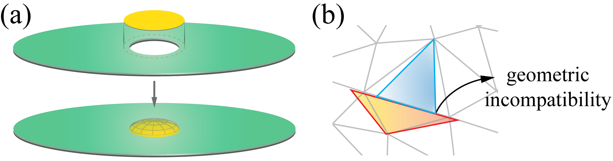
Figure 1: (a) Inserting an elastic disk into an aperture smaller than disk’s size (top) induces residual stress in the disk due to compression. This residual stress can be released by buckling out of plane (bottom). (b) In a discrete picture where an elastic sheet is represented as a triangulation of a surface, the geometric incompatibility leading to the residual stress (i.e., non-embeddable metric) can be understood as two triangles that share an edge having mutually incompatible preferred shapes, e.g. red (blue) triangle is the preferred shape for the corresponding grey mesh triangle shown underneath it.

In this paper, we study thin elastic and viscoelastic sheets with activity introduced as a dynamical change of the reference shape. Physically, activity provides structural remodelling that acts as a local time-dependent source of strain. The time-dependent reference shape can be either stress free (embeddable metric) or contain residual stress (non-embeddable metric) (Efrati et al., 2009). While the distinction between the two cases has important consequences for the elastic ground state (Efrati et al., 2009; Kang et al., 2014), it is not essential for the present discussion. As shown in Fig. 1, bending out of plane can fully or partly remove the residual stresses due to remodelling, depending on whether the particular reference state is embeddable or not in $\mathbb{R}^{3}$. It has been recently argued (Clément et al., 2017) that viscoelastic relaxation can stabilise cell shapes during morphogenesis. Such viscoelastic effects remove all stresses over a sufficiently long time. Here, we focus on the regime where active remodelling is faster than both elastic and viscoelastic relaxation, leading to the system being inherently out of equilibrium. This regime is expected to be of particular importance to early embryonic development.

We study a thin sheet of size $L$ and uniform thickness $h\ll L$ with linear elastic response (Audoly and Pomeau, 2010). We assume that the surrounding fluid provides damping but ignore all other hydrodynamic effects. The sheet is represented by the two-dimensional mid-surface, initially in the $xy$ plane. The deformed mid-surface with no overhangs can be parametrised as $\mathbf{r}=\mathbf{r}\left(x,y\right)=\left(x,y,w\left(x,y\right)\right)$, where $w\left(x,y\right)$ is a sufficiently smooth height function. One defines the metric, $g_{\alpha\beta}=\partial_{\alpha}\mathbf{r}\cdot\partial_{\beta}\mathbf{r}$, and curvature, $c_{\alpha}^{\beta}=g^{\beta\gamma}b_{\alpha\gamma}$, tensors where $b_{\alpha\beta}=-\partial_{\alpha}\mathbf{r}\cdot\partial_{\beta}\mathbf{n}$ ($\alpha,\beta\in\left\{x,y\right\}$) is the second fundamental form and $\mathbf{n}=\left(\partial_{x}\mathbf{r}\times\partial_{y}\mathbf{r}\right)/\left|\partial_{x}\mathbf{r}\times\partial_{y}\mathbf{r}\right|$ is the unit normal vector (Do Carmo, 1976) (Fig. 2a). The elastic energy of the mid-surface is (Koiter, 1966; Efrati et al., 2009; SI, )

$$E=\int dA\mathcal{A}^{\alpha\beta\gamma\delta}\left(\frac{h}{2}u_{\alpha\beta}u_{\gamma\delta}+\frac{h^{3}}{24}b_{\alpha\beta}b_{\gamma\delta}\right),$$ (1)

where $u_{\alpha\beta}=\frac{1}{2}\left(g_{\alpha\beta}-\overline{g}_{\alpha\beta}\right)$ is the strain tensor, $\overline{g}_{\alpha\beta}$ is a reference metric tensor, $dA=\sqrt{\det g}dxdy$ is the area element, $\mathcal{A}^{\alpha\beta\gamma\delta}$ is the elastic tensor, and summation over pairs of repeated indices is assumed. Latin indices refer to the components of vectors in the embedding Euclidean $\mathbb{R}^{3}$ space, while Greek indices are used to label intrinsic curvilinear coordinates. For an isotropic material, $\mathcal{A}^{\alpha\beta\gamma\delta}=\frac{Y}{1+\nu}\left(\frac{\nu}{1-\nu}\overline{g}^{\alpha\beta}\overline{g}^{\gamma\delta}+\overline{g}^{\alpha\gamma}\overline{g}^{\beta\delta}\right)$, where $Y$ is the Young’s modulus and $\nu$ is the Poisson ratio and $\overline{g}^{\alpha\gamma}\overline{g}_{\gamma\beta}=\delta_{\beta}^{\alpha}$. The first term in Eq. (1) is the stretching energy and the second term accounts for bending. For an isotropic material, stretching and bending energies simplify to $E_{s}=\frac{h}{2}\int dA\frac{Y}{1+\nu}\left(\frac{\nu}{1-\nu}u_{\alpha}^{\alpha}u_{\beta}^{\beta}+u_{\alpha}^{\beta}u_{\beta}^{\alpha}\right)$ and $E_{b}=\frac{h^{3}}{24}\int dA\frac{Y}{1+\nu}\left(\frac{\nu}{1-\nu}c_{\alpha}^{\alpha}c_{\beta}^{\beta}+c_{\alpha}^{\beta}c_{\beta}^{\alpha}\right)$, with $u_{\alpha}^{\beta}=\overline{g}^{\beta\gamma}u_{\alpha\gamma}$ and $c_{\alpha}^{\beta}=\overline{g}^{\beta\gamma}b_{\alpha\gamma}$ (Efrati et al., 2009; SI, ). With the mean curvature $H=\frac{1}{2}c_{\alpha}^{\alpha}\equiv\frac{1}{2}\text{Tr}\left(\hat{c}\right)$ and the Gaussian curvature $K=\det\left(c_{\alpha}^{\beta}\right)$, the bending energy becomes $E_{b}=\int dA\kappa\left(2H^{2}-\left(1-\nu\right)K\right)$, where $\kappa=h^{3}Y/12\left(1-\nu^{2}\right)$ is the bending stiffness. In general, material properties and the reference metric can be position dependent and the sheet can have a spontaneous curvature, $H_{0}$. Here we assume that $H_{0}=0$ and the active remodelling does not affect elastic parameters. In reality, material properties are affected by the structural remodelling. However, imposing spatial and time dependence on the elastic parameters did not qualitatively change our findings and, for simplicity, in following we assume them be constant. Finally, we estimate that the relaxation time associated with bending, $\tau_{el}\sim\eta L^{3}/\kappa$, here $\eta$ is the dynamical viscosity of the surrounding fluid (SI, ). For an epithelial cell sheet in water, $\tau_{el}\sim 10^{1}-10^{2}$ s, consistent with (Marmottant et al., 2009). Clearly, the time scale of relaxation associated with stretching deformation is much shorter and consequently of no importance for the present discussion.

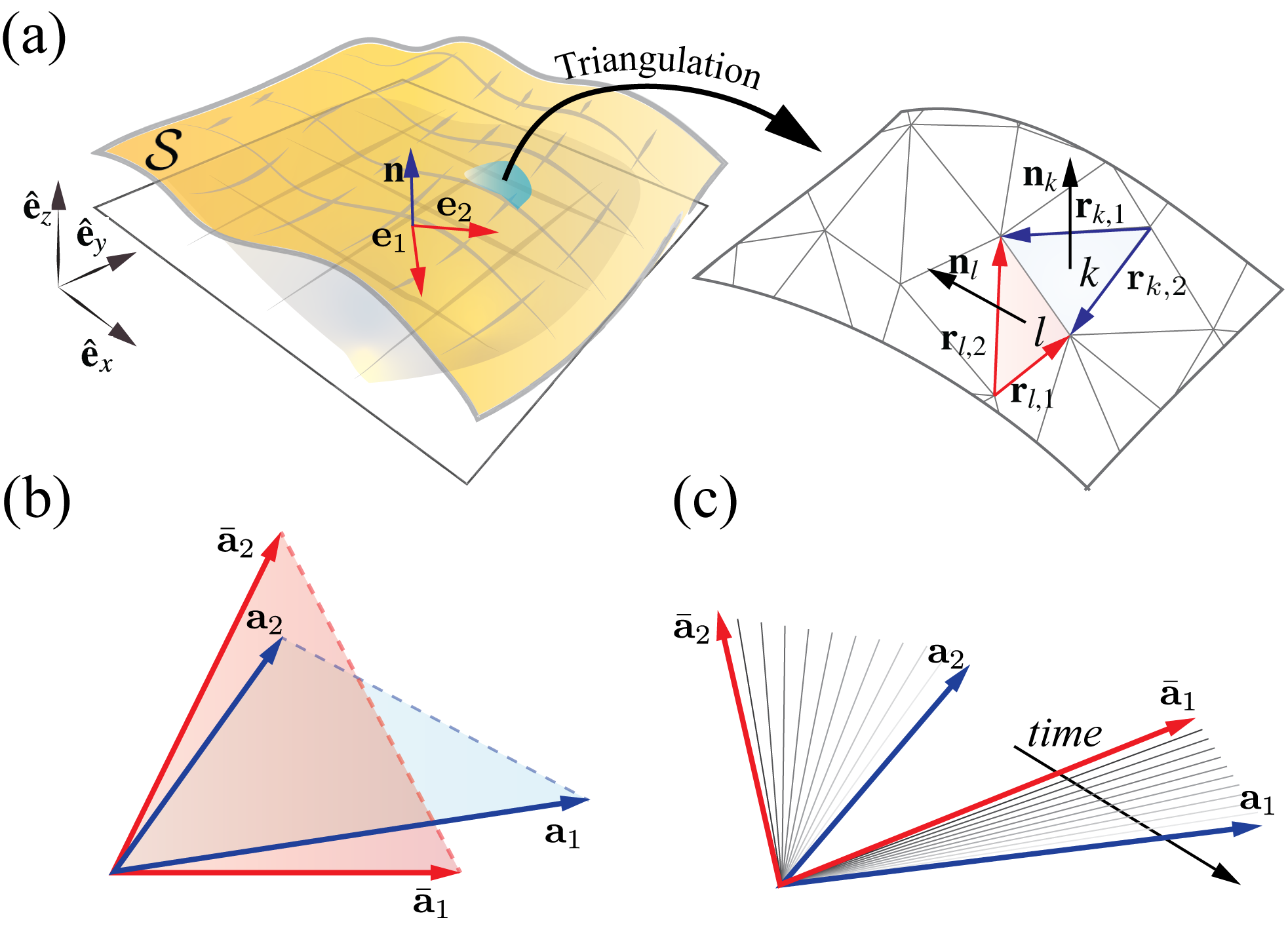
Figure 2: (a) The sheet is represented as a two-dimensional mid-surface parametrised by $\left(x,y\right)-$coordinates, with two tangent vectors ($\mathbf{e}_{1}\equiv\partial_{x}\mathbf{r}$, $\mathbf{e}_{2}\equiv\partial_{y}\mathbf{r}$) and a unit-length normal $\left(\mathbf{n}=\left(\mathbf{e}_{1}\times\mathbf{e}_{2}\right)/\left|\mathbf{e}_{1}\times\mathbf{e}_{2}\right|\right)$ assigned to each point of the surface. For numerical implementation, the surface is discretised in terms of triangles. (b) Red vectors form the reference metric tensor, $\bar{g}_{\alpha\beta}=\bar{\mathbf{a}}_{\alpha}\cdot\bar{\mathbf{a}}_{\beta}$ and blue vectors form the realised metric tensor, $g_{\alpha\beta}=\mathbf{a}_{\alpha}\cdot\mathbf{a}_{\beta}$. The strain tensor is defined as $u_{\alpha\beta}=\frac{1}{2}\left(g_{\alpha\beta}-\overline{g}_{\alpha\beta}\right)$. (c) Viscoelasticity is modelled as a relaxation of the reference metric towards the realised metric, with a characteristic time scale $\tau_{v}$.

Active effects in a tissue result, for example, from myosin driven contractions and turnover of the actin cytoskeleton (Joanny and Prost, 2009) as well as cell growth and division. Processes related to the cytoskeleton typically occur at time scales of $\tau_{a}\sim 10^{1}-10^{2}$ s (Rauzi et al., 2008, 2010), while cell growth and division are slower and can span several hours (Alberts et al., 2014). Dissipation in tissues results from multi-cellular rearrangements (i.e., plastic events such as intercalations, ingressions and extrusions) and sub-cellular cytoskeleton remodelling (i.e., cell shape relaxation). We note that dissipation is accompanied by entropy production and, in general, an entropy production equation would be required (Salbreux and Jülicher, 2017). Here, we are not concerned by the details of the dissipative processes (rendering the entropy production equation unnecessary) and assume that they occur on a time scale, $\tau_{v}$. We note, however, that cell rearrangements are typically slower (occurring on the scale $\sim 10$ min) than the sub-cellular remodelling (occurring on the seconds to minutes scale). While it is not always the case, the out of equilibrium situation with $\tau_{a}<\tau_{el},\tau_{v}$ is, therefore, biologically plausible and, we argue, beneficial to access diversity of shapes needed to form complex structures. In the following, we explore the range of possible dynamical shape patterns formed in the non-equilibrium regime.

The advantage of expressing deformation with respect to the reference metric (Sknepnek and Olvera de la Cruz, 2012) is that the formalism can be directly generalised to include active remodelling and viscoelastic relaxation, without making only assumptions about the existence of a stress free reference state. Here, active remodelling is introduced by imposing dynamical changes of the reference metric. The precise functional form of active remodelling is not important, as long as one can associate a typical time scale, $\tau_{a}$, to it. Active remodelling can be thought of as a generalisation of growth, with the quasi-static differential growth being described as $\bar{g}_{\alpha\beta}\left(\mathbf{r},t\right)=a\left(\mathbf{r}\right)t\bar{g}_{\alpha\beta}\left(\mathbf{r},t=0\right)$, where $a\left(\mathbf{r}\right)>0$ and $\tau_{a}^{growth}\equiv a^{-1}\ll\tau_{el}$. We model viscoelastic effects as a relaxation of the reference metric towards the realised metric (Fig. 2c). Therefore, viscoelastic relaxation has the opposite effect of elasticity, for which the reference state conforms to the realised shape rather than the other way around. A description based on the time-evolving reference metric is also suitable for direct discretisation (Fig. 2) and efficient parallel implementation on GPUs (SI, ). This allows us to simulate systems containing up to $2\times 10^{6}$ triangles removing the need to implement complex remeshing procedures to avoid reduction in accuracy in the vicinity of high-curvature folds.

We assume overdamped dynamics and solve the set of first-order equations for each vertex $i$ and discrete metric of each triangle,

$$\gamma\dot{\mathbf{r}}_{i} =-\nabla_{\mathbf{r}_{i}}E\left(g_{\alpha\beta},\bar{g}_{\alpha\beta},b_{\alpha\beta}\right)+\boldsymbol{\eta}_{i}\left(t\right),$$ (2a)

$$\dot{\bar{g}}_{\alpha\beta}\left(\mathbf{r},t\right) =R_{\alpha\beta}\left(\overline{g}_{\alpha\beta},t\right)+V_{\alpha\beta}^{\gamma\delta}\left(t\right)\left(g_{\gamma\delta}\left(\mathbf{r},t\right)-\bar{g}_{\gamma\delta}\left(\mathbf{r},t\right)\right).$$ (2b)

Here $\mathbf{r}_{i}\in\mathbb{R}^{3}$ is the position vector of vertex $i$, $\boldsymbol{\eta}_{i}\left(t\right)\in\mathbb{R}^{3}$ is a weak random noise, obeying $\left\langle\boldsymbol{\eta}_{i}\right\rangle=0$ and $\left\langle\eta_{i}^{m}\left(t\right)\eta_{j}^{n}\left(t^{\prime}\right)\right\rangle=\sqrt{2\gamma k_{B}T}\delta_{ij}\delta_{mn}\delta\left(t-t^{\prime}\right)$ with $m,n\in\left\{x,y,z\right\}$. $\gamma$ is the friction coefficient modelling dissipation by the surrounding fluid and $T$ is the temperature kept very low and used only for numerical convenience to avoid being trapped in shallow local minima. All our simulations were effectively at $T=0$ as thermal fluctuations are not expected to play an appreciable role in biological systems, i.e., relevant energy scales far exceed $k_{B}T$. $V_{\alpha\beta}^{\gamma\delta}$$\left(t\right)$ is a tensor that sets the rate of viscous relaxation. While in general $V_{\alpha\beta}^{\gamma\delta}$ is a function of time, here we assume it to be constant, $V_{\alpha\beta}^{\gamma\delta}=\frac{1}{\tau_{v}}\delta_{\alpha}^{\gamma}\delta_{\beta}^{\delta}$. $R_{\alpha\beta}$ is a tensor function that prescribes active remodelling rate. Here, $R_{\alpha\beta}$ models metric expansion and is given in Eq. (S34) in (SI, ). Furthermore, $R_{\alpha\beta}$ explicitly depends on time and, thus, models dynamical changes of the active remodelling rate. Finally, discrete versions of the realised and reference metric tensors are defined in Fig. 2b. Eqs. (2a) and (2b) are integrated numerically using standard first-order Euler-Maruyama discretisation scheme keeping connectivity of the triangulation fixed. Expressions for the gradient of energy in Eq. (2a) are straightforward but lengthy (SI, ). Note that in the current implementation, we do not include steric effects and the sheet can take unphysical self-intersecting configurations. Including self-avoidance is possible but technically challenging to efficiently implement on GPUs. Steric effect would indeed affect the folding patterns but would not change our main conclusions. Values of parameters used in simulations are given in (SI, ). Moreover, length is measured in units of $h$, time in units of $t^{*}=\gamma/Yh$ and energy in units of $\kappa$.

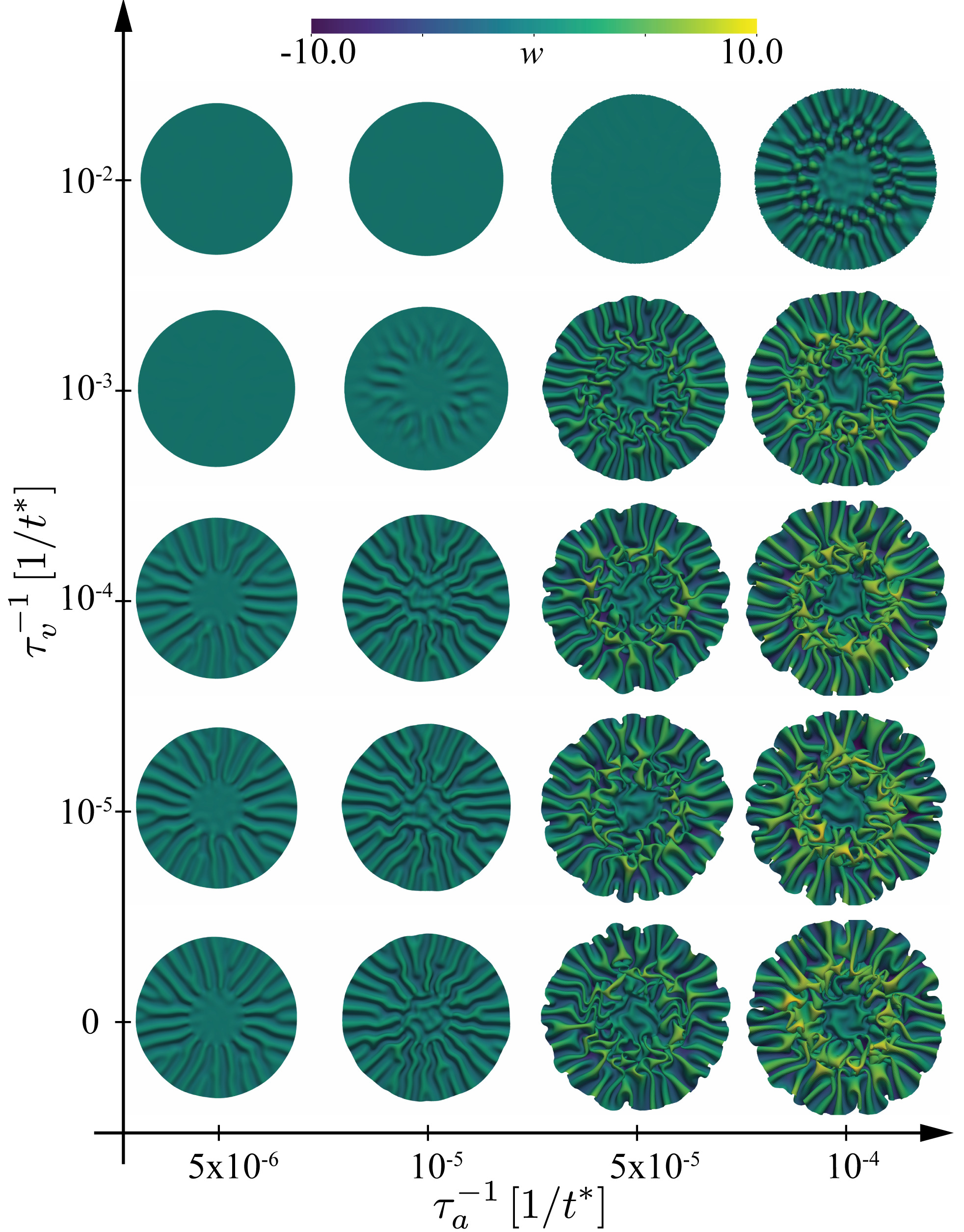
Figure 3: A snapshot of the out-of equilibrium shapes obtained by numerical integration of Eqs. (2a) and (2b) starting from a flat disk configuration. The snapshots are taken at $t=10^{4}t^{*}$. Vertical axis represents the rate of viscous (dissipative) relaxation with increasing values designating faster residual stress relaxation. On the horizontal axis we plot the active structural remodelling rate, with larger values corresponding to faster changes of the local reference metric. The usual slow, quasi-equilibrium elastic growth would correspond to the lower left corner in this graph. Colours represent the height function, $w\left(x,y\right)$. In these simulations, $R_{\alpha\beta}$ is time independent.

We explored out of equilibrium dynamics of flat disks of radius $R$ subject to active remodelling and viscous dissipation (Fig. 3). The choice of the disk geometry is inspired by extensive work on wrinkling patterns due to tension (Jagla, 2007; Davidovitch et al., 2011) or resulting from a quasi-equilibrium growth, e.g., during biofilm formation (Amar and Wu, 2014; Yan et al., 2019). This regime corresponds to $\tau_{el}\ll\tau_{a}$. We assume that a ring of radius $r_{i}<R$ is kept fixed but can transmit stress. Active remodelling is assumed to occur only in the outer annulus, for $r_{i}<r<R$. With no viscoelastic relaxation and slow active remodelling (lower left corner in Fig. 3), the system is in the extensively studied quasi-equilibrium differential growth regime. Free expansion of the outer boundary can relieve part of the stress produced by growth. There is, however, no such stress relief mechanism in the tangential direction and the sheet forms a regular pattern of radial wrinkles. The inner disk, on the other hand, is compressed in both directions leading to wrinkles with no preferred orientation. If one instead allows for viscoelastic relaxation while keeping the active remodelling slow (left column in Fig. 3), wrinkles are less pronounced or, in the case of very fast dissipative relaxation, do not form at all (top left in Fig. 3). This is easy to understand, as in this regime the stress generated by active remodelling is dissipated by a fast relaxation of the reference metric of the sheet. As one increases the remodelling rate (second and third columns in Fig. 3), wrinkling patterns become more pronounced and less regular, especially close to the inner ring, where stress accumulation is strong. Without viscous dissipation (bottom right in Fig. 3) the sheet continues to expand and quickly reaches unphysical self-intersecting configurations. In a real system, steric repulsion and intrinsic biological processes such as apoptosis due to hypoxia and nutrient deprivation would prevent this uncontrolled growth. If viscoelastic relaxation is introduced, the stress generated by active remodelling is in part dissipated, which prevents wrinkles from growing rapidly (upper right region in Fig. 3). The ratio between active relaxation and viscous dissipation then determines the steady state wrinkling patterns. These patterns, however, do not correspond to minima of elastic energy and thus exhibit far richer morphologies compared to the equilibrium states (Fig. S1 in (SI, )).

Furthermore, if the system is able to dynamically tune the active remodelling rate, it can reach conformations that would otherwise require ovecoming large energy barriers. For example, for a fixed high value of $\tau_{a}^{-1}$, one needs to inject substantial energy in order to initiate wrinkling (Fig. S1, circles). On the other hand, if the initial value of $\tau_{a}^{-1}$ is reduced, the wrinkling energy barrier is significantly lowered (Fig. S1, triangles). This is not surprising as elastic relaxation is not fast enough to accommodate structural changes due to fast active remodelling. If $\tau_{a}^{-1}$ is increased once the wrinkles are formed, however, it is easy to reach different wrinkling patterns (Fig. S1 pentagons) without the high initial energy cost. This simple example shows that an out of equilibrium system is not only able to develop a rich variety of morphologies but it also can avoid costly energy barriers between different patterns by dynamically tuning its parameters, which most biological systems are equipped to do.

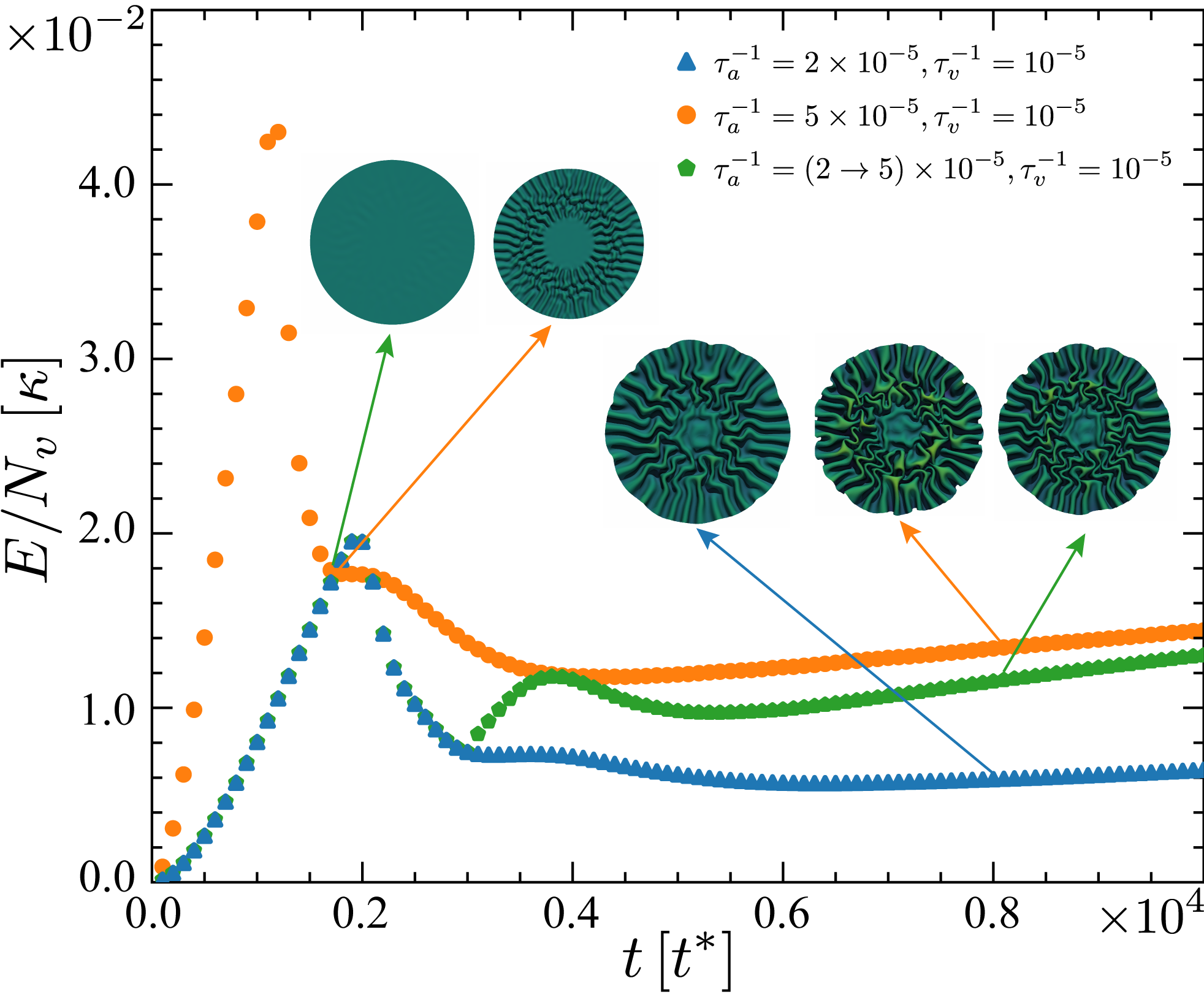
Figure 4: Energy per vertex as a function of simulation time. To reach a wrinkled configuration with a remodelling rate $\tau_{a}^{-1}=5\times 10^{-5}$ would require the sheet to overcome a large energy barrier (peak of the orange curve). If the initial remodelling rate, however, is set to $\tau_{a}^{-1}=2\times 10^{-5}$, the system requires less energy to reach the wrinkling instability (peak of the blue curve). Upon switching to $\tau_{a}^{-1}=5\times 10^{-5}$ at $t=1.7\times 10^{4}t^{*}$, the evolution continues along the green curve and the system reaches a wrinkling pattern, which is very similar to the one obtained by following the orange curve, as shown by the two snapshots on the right. All rates are given in units of $1/t^{*}$.

By applying an active solid model to viscoelastic thin sheets subject to active structural remodelling, we showed that the interplay between activity and viscous relaxation leads to a diverse morphology of out of equilibrium wrinkling patterns. Of particular interest in this study is the regime where active processes are faster than elastic and viscoelastic relaxation. In this case, the system has no time to fully relax local stresses produced by active remodelling allowing local perturbations to grow. As a consequence, the shape patterns depend on the initial conditions and local fluctuations. This is in stark contrast to the mechanics of growth, in particular in plants, that has been extensively studied with great success (Goriely, 2017). Most theoretical approaches are based on continuum mechanics augmented to encode the effects of growth into Föppl-von Kármán equations (Amar and Goriely, 2005; Goriely and Amar, 2005, 2007). The salient point in such treatments is that elastic relaxation occurs at the time scales that are short compared to growth and thus describe the regime where the system is always in quasi-static mechanical equilibrium (Rodriguez et al., 1994; Amar and Goriely, 2005). We argue that the out of equilibrium regime studied here is of particular interest in developing physical understanding of morphogenesis.

We note that a similar observation has been recently made in a study of the dynamics of growth and form in prebiotic vesicles (Ruiz-Herrero et al., 2019) where the observed diversity of shapes was associated with the imbalance of surface and volume growth and the rate of relaxation. This suggests that keeping a growing system out of equilibrium significantly increases the range of available morphologies. The development of higher organisms is too complex to be captured by a simple mechanical model of actively remodelling sheets. Our observations, however, point to a mechanism by which a system that is kept out of equilibrium could be steered towards a desired shape by a careful regulation of remodelling, relaxation and mechanical parameters. This would be much easier to encode in the space available in the genome.

RS would like to thank C. J. Weijer for his valuable insights into developmental biology. FD, NSW and DMF were funded by the UK BBSRC (Award BB/P001335/1). RS acknowledges support by the UK BBSRC (Award BB/N009789/1).

Supplemental Materials: Wrinkle patterns in active viscoelastic thin sheets

I Energy

Here we show the elastic energy for different value of $\tau_{a}^{-1}$ and $\tau_{v}^{-1}$. Fig. S1 shows that the elastic energy is far from the global minimum with prominent regions of highly concentrated bending energy. If viscoelastic relaxation is introduced, the stress generated by active remodelling is in part dissipated, which prevents wrinkles from growing rapidly (upper right region in Fig. 3 main text). The ratio between active relaxation and viscous dissipation then determines the steady state wrinkling patterns. These patterns, however, do not correspond to minima of elastic energy and thus exhibit far richer morphologies compared to the equilibrium states. It is also easy to transition between different wrinkling patterns by tuning system parameters, which most biological systems are equipped to do. Note that while the precise morphology of wrinkling patterns depends on the geometry of the system, the mechanism that leads to such out of equilibrium structures does not.

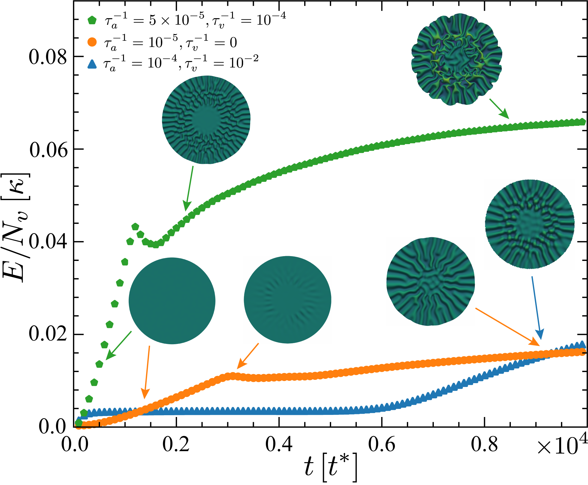
Figure S1: Total elastic energy $E$ divided by the number of vertices $N_{v}$ as a function of the simulation time. Note that small peaks in the green and orange curves correspond to the onset or wrinkling. The sheet represented by the blue curve wrinkles at around $t=60t^{*}$, however, there is no distinct peak due to very strong viscous relaxation. Once the wrinkles form, the energy gradually increases due to active remodelling. Note that within our model, in most cases, the system would not reach a steady state and different mechanism would have to be introduced to stabilise the system. $\tau_{a}^{-1}$ and $\tau_{v}^{-1}$ are measured in units of $t^{*-1}$.

II Other geometries and remodelling tensors

Here we show two examples of geometries and structural remodelling. The first example (Fig. S2) shows the case of a strip of size $L_{x}=100$ and $L_{y}=20$ under uniform structural and viscous remodelling. As in the case of Fig. 3 in the main text, if one increase the rate of viscoelastic relaxation while keeping the active remodelling wrinkles are less pronounced or, in the case of very fast dissipative relaxation, do not form at all.

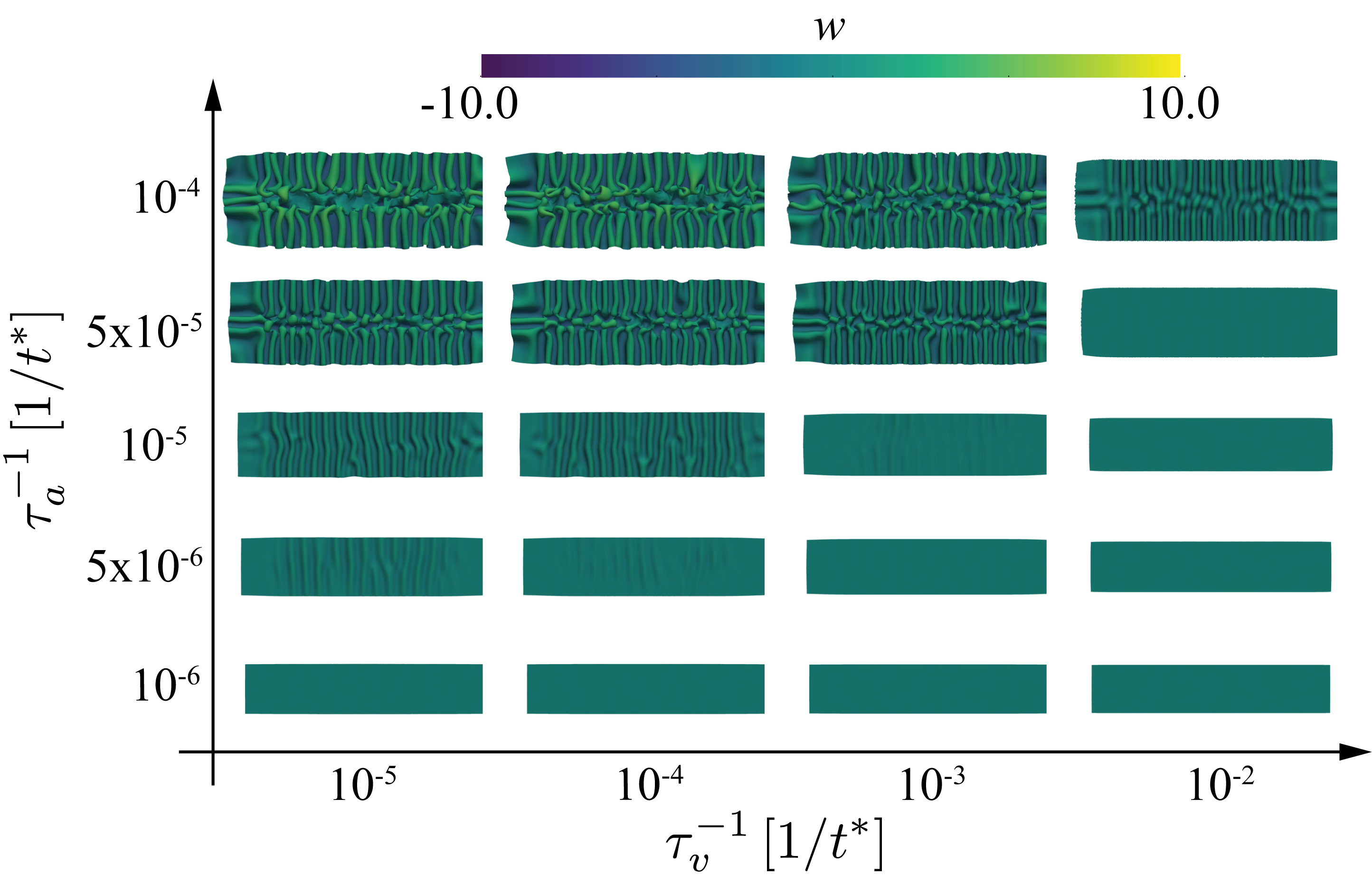
Figure S2: A snapshot of the out-of equilibrium shapes obtained by numerical integration of Eqs. (2) and (3) in the main text starting from a flat stripe configuration. The snapshots are taken at $t=4\times 10^{3}t^{*}$. Horizontal axis represents the rate of viscous (dissipative) relaxation with increasing values designating faster residual stress relaxation. On the vertical axis we plot the active structural remodelling rate, with larger values corresponding to faster changes of the local reference metric. The usual slow, quasi-equilibrium elastic growth would correspond to the lower left corner in this graph. Colours represent the height function, $w\left(x,y\right)$.

The second example (Fig. S3), mimics active compression of a flat disk of size $R=50$. The compression is introduced by imposing a rapid strain trough an instantaneous change on the reference metric in an external annulus $0.8R<r<R$. Viscous remodelling is assumed to occur only in the inner annulus, for $r<0.8R$.

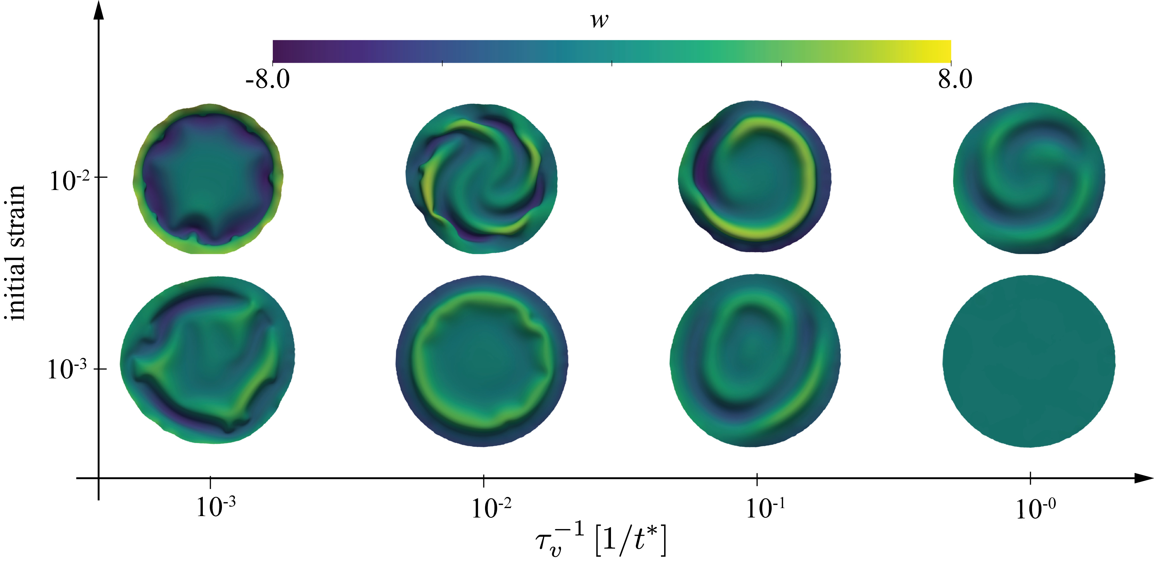
Figure S3: A snapshot of the out-of equilibrium shapes obtained by numerical integration of Eqs. (2) and (3) in the main text starting from a flat stripe configuration. The snapshots are taken at $t=2\times 10^{4}t^{*}$. Horizontal axis represents the rate of viscous (dissipative) relaxation with increasing values designating faster residual stress relaxation. On the vertical axis, we plot the initial residual strain in the exterior annulus, with larger values corresponding to larger changes of the local reference metric. Colours represent the height function, $w\left(x,y\right)$.

III Elasticity

Starting for the energy expression for a thin three-dimensional solid we derive energy expression for its two-dimensional neutral surface. The neutral surface is placed midway along the thin direction (see Fig. S4) and on it bending and stretching are decoupled.

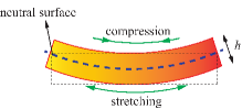
Figure S4: A perpendicular cut through a thin sheet of thickness $h\ll 1$. As the sheet is bend upwards from its rest configuration (dashed black lines) it deforms. The inner side (towards the direction of the bend) gets compressed while the outer side becomes stretched. It is clear that as one moves away from the inner side towards the outer side the amount of compression decreases and eventually turns into stretching. Therefore, there is a surface which neither stretches nor compresses, the so-called neutral surface (blue dashed line) and is clearly exactly in the middle of the sheet.

III.1 Strain tensor

A point at position $\mathbf{r}$ under the deformation is displaced to (Green, )

$$\mathbf{r}^{\prime}=\mathbf{r}+\mathbf{u},$$ (S1)

where vector $\mathbf{u}\left(\mathbf{r}\right)$ is the displacement vector. The elastic energy of the body cannot depend on actual displacement but it depends on the derivatives of $\mathbf{u}$. In other words, the elastic energy depends on the changes in the metric of the body. We define the strain tensor

$$u_{ij}=\frac{1}{2}\left(g_{ij}-\bar{g}_{ij}\right).$$ (S2)

If we recall that

$$\bar{g}_{ij}=\partial_{i}\mathbf{r}\cdot\partial_{j}\mathbf{r}=\mathbf{e}_{i}\cdot\mathbf{e}_{j},$$

and

$$\begin{split}g_{ij}&=\bar{g}_{ij}+\mathbf{e}_{i}\cdot\partial_{j}\mathbf{u}+\mathbf{e}_{j}\cdot\partial_{i}\mathbf{u}+\partial_{i}\mathbf{u}\cdot\partial_{j}\mathbf{u},\end{split}$$

the strain tensor becomes

$$u_{ij}=\frac{1}{2}\left(\nabla_{j}u_{i}+\nabla_{i}u_{j}+\nabla_{i}u_{s}\nabla_{j}u^{s}\right),$$ (S3)

where $\nabla_{j}$ is the covariant derivative. In the Euclidean space, $\nabla_{i}=\partial_{i}$, and the last expression reduces to the familiar definition of the strain tensor defined in standard text books on elasticity

$$u_{ij}=\frac{1}{2}\left(\partial_{i}u_{j}+\partial_{j}u_{i}+\partial_{i}u_{s}\partial_{j}u^{s}\right).$$ (S4)

III.2 Three-dimensional elastic energy density

The elastic energy density depends on the strain tensor, i.e., on the metric, $E_{el}=E_{el}\left(g_{ij}\right)$. If the strain is small we can expand $E_{el}$ in powers of $u_{ij}$ around the reference configuration ($\bar{g}_{ij}$ and $u_{ij}=0$)

$$\begin{split}E_{el}&\approx E\left(\bar{g}_{ij}\right)+\left.\frac{\partial E}{\partial g_{ij}}\right|_{u_{ij}=0}u_{ij}+\frac{1}{2}\left.\frac{\partial^{2}E}{\partial g_{ij}\partial g}\right|_{u_{ij}=0}u_{ij}u_{kl}\\ &+o\left(u^{3}\right)\\ &=E\left(\bar{g}_{ij}\right)+\frac{1}{2}A^{ijkl}u_{ij}u_{kl}+o\left(u^{3}\right),\end{split}$$

where we assumed the linear term in the expansion vanishes and introduced a contravariant elastic tensor $A^{ijkl}=\left.\frac{\partial^{2}E}{\partial g_{ij}\partial g_{kl}}\right|_{u_{ij}=0}$. We can omit the unimportant constant term $E\left(\bar{g}_{ij}\right)$ to obtain the expression for elastic energy density in the small strain approximation

$$E_{el}=\frac{1}{2}A^{ijkl}u_{ij}u_{kl}.$$ (S5)

We need to make a distinction between small strain and small displacement approximations, that is, one does not imply the other. If the strains are small and the elastic response of the body is directly proportional to the applied stress, the small strain approximation is applicable and Eq. (S5) is valid, i.e. constitutive laws are linear (Hookean elasticity). However, when studying thin shells, we can have a situation that although strains are small displacements are large. In this case Eq. (S5) is still valid, but we cannot omit nonlinear terms in $u_{ij}$ and we have to use Eq. (S3).

Total elastic energy is Koiter ; Efrati ,

$$E_{tot}=\frac{1}{2}\int_{V}\sqrt{\left|g\right|}A^{ijkl}u_{ij}u_{kl}.$$ (S6)

For an isotropic body there the elastic tensor has only two independent components and can be written as (e.g., Ref. (Efrati, ))

$$A^{ijkl}=\lambda g^{ij}g^{kl}+\mu\left(g^{ik}g^{jl}+g^{il}g^{jk}\right),$$

where $\lambda$ and $\mu$ are two Lame coefficients. We can introduce Young’s modulus $E$ and Poisson’s ratio $\nu$ via

$$\begin{split}E&=\frac{\mu\left(3\lambda+2\mu\right)}{\lambda+\mu}\\ \nu&=\frac{\lambda}{2\left(\lambda+\mu\right)}.\end{split}$$

III.3 Two-dimensional plate Energy density

Expression of the elastic energy density of the neutral surface can be derived (Koiter2, ) under the Kirchhoff-Love assumptions (Refs. (Koiter2, ) and (Efrati, )):

1. Body is in the state of plane-stress, i.e., stress normal to the surfaces parallel to the neutral surface can be neglected.

2. Points which lie on a normal to the neutral surface in the reference configuration remain on the same normal in the deformed configuration.

These assumptions translate into

$$\sigma^{i3}=0\,\,\,\,\,\,i=x,y,z$$ (S7)

where $\sigma^{ij}$ is the contravariant stress tensor, and

$$g_{ij}=\left(\begin{array}[]{cc}g_{\alpha\beta}&0\\ 0&1\end{array}\right)\,\,\,\,\mathrm{or\,\,\,\,\epsilon_{\alpha 3}=0.}$$ (S8)

From Eqs. (S7) and (S8) we have

$$u_{3}^{3}=u_{33}=-\frac{\lambda}{\lambda+2\mu}u_{\alpha}^{\alpha}.$$ (S9)

The elastic energy density in Eq. (S5) can be now rewritten as

$$\begin{split}E_{tot}^{2D}&=\frac{1}{2}\mathcal{A}^{\alpha\beta\gamma\delta}u_{\alpha\beta}u_{\gamma\delta},\end{split}$$

where the two-dimensional elastic tensor is

$$\mathcal{A}^{\alpha\beta\gamma\delta}=2\mu\left(\frac{\lambda}{\lambda+2\mu}g^{\alpha\beta}g^{\gamma\delta}+g^{\alpha\gamma}g^{\beta\delta}\right).$$ (S10)

Using the Kirchhoff-Love assumptions effectively decouples different sheets parallel to the neutral surface (Koiter, ). Therefore, we can obtain the expression for the total elastic energy of the neutral surface by integrating along the sheet thickness (chosen to be the $z$ direction),

$$\begin{split}E_{tot}^{2D}&=\frac{1}{2}\int_{S}\int_{-\frac{h}{2}}^{\frac{h}{2}}dz\sqrt{\left|g\left(z\right)\right|}\mathcal{A}^{\alpha\beta\gamma\delta}u_{\alpha\beta}\left(z\right)u_{\gamma\delta}\left(z\right).\end{split}$$

In the small strain approximation, we can neglect all terms that are are cubic or higher power in $u_{\alpha\beta}$ to get

$$E_{tot}^{2D}=\int_{S}\sqrt{\left|g\right|}\mathcal{A}^{\alpha\beta\gamma\delta}\left(\frac{h}{2}u_{\alpha\beta}u_{\gamma\delta}+\frac{h^{3}}{24}b_{\alpha\beta}b_{\gamma\delta}\right),$$ (S11)

where $b_{ij}=\mathbf{e_{i}}\cdot\partial_{j}\mathbf{n}$ is the second fundamental form, related to the curvature tensor $c_{i}^{j}=g^{ik}b_{kj}$ (doCarmo, ). Eq. (S11) is the expression for the elastic energy of a thin shell expressed in terms of its neutral surface. The first term in the two-dimensional energy expression is stretching energy and it describes energy penalty of stretching or compressing of the neutral surface. The second term is the bending energy, which describes energy penalty of flexing the sheet. We can write $E^{2D}=E_{stretch}+E_{bend}$ where

$$E_{stretch}=\frac{Y}{2\left(1+\nu\right)}\left(\frac{\nu}{1-\nu}u_{\alpha}^{\alpha}u_{\beta}^{\beta}+u_{\beta}^{\alpha}u_{\alpha}^{\beta}\right),$$ (S12)

and $Y=Eh$. Similarly, using $\mathrm{Tr}\left(b_{\alpha}^{\beta}\right)=2H$ and $\mathrm{Tr}\left(\left(b_{\mu}^{\gamma}\right)^{2}\right)=4H^{2}-2K$,

$$\begin{split}E_{bend}&=\frac{h^{3}}{24}\frac{E}{\left(1+\nu\right)}\left(\frac{\nu}{1-\nu}b_{\alpha}^{\alpha}b_{\gamma}^{\gamma}+b_{\alpha}^{\beta}b_{\beta}^{\alpha}\right)\\ &=2\kappa H^{2}+\kappa_{G}K,\end{split}$$ (S13)

with the bending modulus, $\kappa=Eh^{3}/12\left(1-\nu^{2}\right)$ and Gaussian modulus $\kappa_{G}=-Eh^{3}/12\left(1+\nu\right)$.

IV Discrete model

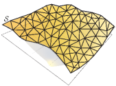
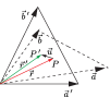
Figure S5: (Left) Discrete model of a thin sheet modelled as a two-dimensional surface. The surface is represented as a set of vertices connected by edges to form triangles. (Right) A point $P$ described by vector $\mathbf{r}$ in the undeformed (reference) triangle spanned by vectors $\mathbf{a}$ and $\mathbf{b}$ is moved to the point $P\,^{\prime}$ with vector $\mathbf{r}\,^{\prime}$ in the deformed triangle, spanned by vectors $\mathbf{a}^{\prime}$ and $\mathbf{b}^{\prime}$.

We discretise the surface using a triangular mesh (Seung, ), Fig. S5.

IV.1 Stretching energy

We start with the stretching energy term. Closely following Ref. (Parrinello, ), coordinates of a given point $P$ inside a triangle can be written in terms of the two vectors $\mathbf{a}$ and $\mathbf{b}$ (Fig. S5),

$$\mathbf{r}=\xi\mathbf{a}+\eta\mathbf{b},$$ (S14)

where $0\leq\xi\leq 1$ and $0\leq\eta\leq 1$ are coordinates of vector $\mathbf{r}$ in the basis $\left\{\mathbf{a},\mathbf{b}\right\}$. Note that vectors $\mathbf{a}$ and $\mathbf{b}$ are themselves three dimensional vectors constructed as

$$\begin{split}\mathbf{a}&=\mathbf{r}_{2}-\mathbf{r}_{1},\\ \mathbf{b}&=\mathbf{r}_{3}-\mathbf{r}_{1},\end{split}$$

where $\mathbf{r}_{1}$, $\mathbf{r}_{2}$ and $\mathbf{r}_{3}$ are positions of the three corners of the triangle. For convenience, that is to be able to work with square matrices that are invertible, we will introduce a third vector

$$\mathbf{c}=\mathbf{a}\times\mathbf{b}.$$

We can now construct a $3\times 3$ matrix

$$\hat{h}=\left(\begin{array}[]{cc}\mathbf{a}&\mathbf{b}\end{array}\right)\equiv\left(\begin{array}[]{ccc}a_{x}&b_{x}&c_{x}\\ a_{y}&b_{y}&c_{y}\\ a_{z}&b_{z}&c_{z}\end{array}\right),$$ (S15)

such that

$$\mathbf{r}=\hat{h}\mathbf{s},$$ (S16)

where

$$\mathbf{s}=\left(\begin{array}[]{ccc}\xi&\eta&\omega\end{array}\right)^{T},$$

where $\omega\equiv 0$. In term of coordinates Eq. (S16) can be written as

$$r_{i}=h_{i}^{\alpha}s_{\alpha},$$

and we have used Latin indices to count components in the embedding space and Greek indices to count components of vector $\mathbf{s}$. If we now introduce point $Q$ in the same triangle with coordinates $\phi$ and $\psi$, i.e., with $\mathbf{s}_{Q}=\left(\begin{array}[]{ccc}\phi&\psi&0\end{array}\right)^{T}$ then

$$\mathbf{r}_{Q}=\hat{h}\mathbf{s}_{Q}.$$

Square of the distance $l^{2}$ between points $P$ and $Q$ is

$$\begin{split}l^{2}&=\left(\mathbf{r}_{P}-\mathbf{r}_{Q}\right)\cdot\left(\mathbf{r}_{P}-\mathbf{r}_{Q}\right)\\ &=\left(\mathbf{s}_{\left(P\right)}-\mathbf{s}_{\left(Q\right)}\right)\hat{\bar{g}}\left(\mathbf{s}_{\left(P\right)}-\mathbf{s}_{\left(Q\right)}\right).\end{split}$$

and we have used parentheses in the sub- and superscript to designate that $P$ and $Q$ are not indices and have freely changed the name of the repeated summation indices. Matrix

$$\hat{\bar{g}}=\hat{h}^{T}\hat{h}$$

is the (discrete) metric of our reference triangle. Explicitly,

$$\begin{split}\hat{\bar{g}}&=\left(\begin{array}[]{ccc}\mathbf{a}&\mathbf{b}&\mathbf{c}\end{array}\right)^{T}\left(\begin{array}[]{ccc}\mathbf{a}&\mathbf{b}&\mathbf{c}\end{array}\right),\\ \end{split}$$ (S17)

i.e., matrix $\hat{\bar{g}}$ is a $3\times 3$ matrix with a $2\times 2$ sub-matrix corresponding to the metric tensor of the triangle and the $\mathbf{c}\cdot\mathbf{c}$ term that is added for convenience. Matrix $\hat{\bar{g}}$ can be easily computed.

After the deformation edges of the triangle change and the basis vectors become $\mathbf{a}^{\prime}$ and $\mathbf{b}^{\prime}$, while the point $P$ has moved to the new position $P^{\prime}$ with coordinates

$$\mathbf{R}=\hat{H}\mathbf{s}\,,$$

where $\hat{H}=\left(\begin{array}[]{ccc}\mathbf{a}^{\prime}&\mathbf{b}^{\prime}&\mathbf{c}^{\prime}\end{array}\right)^{T}\left(\begin{array}[]{ccc}\mathbf{a}^{\prime}&\mathbf{b}^{\prime}&\mathbf{c}^{\prime}\end{array}\right)$. Note that we assume that the deformation is linear and as such automatically affine. An important of this restrictions is that the point $P^{\prime}$ has the same coordinates $\left(\xi,\eta,0\right)$ in the deformed triangle $\left\{\mathbf{a}^{\prime},\mathbf{b}^{\prime}\right\}$ as the point $P$ had in the original undeformed state. Point $P^{\prime}$ is point $P$ after deformation. If we recall Eq. (S1) and the definition of the displacement vector

$$\begin{split}\mathbf{u}&=\mathbf{R}-\mathbf{r}\\ &=\hat{H}\hat{h}^{-1}\mathbf{r}-\mathbf{r},\end{split}$$

where in the second line we have inverted Eq. (S16) to get $\mathbf{r}=\hat{h}^{-1}\mathbf{s}$. Finally,

$$\mathbf{u}=\left(\hat{H}\hat{h}^{-1}-\hat{I}\right)\mathbf{r},$$ (S18)

where $\hat{I}$ is the identity matrix. In terms of coordinates we have

$$u^{i}=\left[\left(\hat{H}\hat{h}^{-1}\right)_{j}^{i}-\delta_{j}^{i}\right]x^{j}.$$

In order to derive the expression for the non-linear strain tensor in term of matrices $\hat{H}$ and $\hat{h}$ we use Eq. (S4) repeated for convenience (in a form of a mixed tensor),

$$u_{i}^{j}=\frac{1}{2}\left(\frac{\partial u_{i}}{\partial x^{j}}+\frac{\partial u^{j}}{\partial x_{i}}+\frac{\partial u^{k}}{\partial x_{i}}\frac{\partial u_{k}}{\partial x^{j}}\right).$$ (S19)

Now we compute

$$\begin{split}\frac{\partial u_{i}}{\partial x^{j}}&=\left[\left(\hat{H}\hat{h}^{-1}\right)_{i}^{k}-\delta_{i}^{k}\right]\frac{\partial x_{k}}{\partial x^{j}}\\ &=\left[\left(\hat{H}\hat{h}^{-1}\right)_{i}^{j}-\delta_{i}^{j}\right].\end{split}$$

If we plug the last expression into Eq. (S19) we obtain

$$\begin{split}\hat{u}&=\frac{1}{2}\left[\left(\hat{H}\hat{h}^{-1}\right)^{T}\hat{H}\hat{h}^{-1}-\hat{I}\right]\\ &=\frac{1}{2}\left(\hat{h}^{-T}\hat{g}\hat{h}^{-1}-\hat{I}\right),\end{split}$$ (S20)

where we have used $\left(AB\right)^{T}=B^{T}A^{T}$ and $A^{-T}\equiv\left(A^{-1}\right)^{T}$. We can now use Eq. (S12) to write

$$E_{stretch}=\frac{A_{T}Eh}{8(1+\nu)}\left[\frac{\nu}{1-\nu}\left(\mathrm{tr}\hat{F}\right)^{2}+\mathrm{tr}\left(\hat{F}^{2}\right)\right],$$ (S21)

where $A_{T}$ is the triangle area and the tensor $\hat{F}$ is given by,

$$\hat{F}=\hat{\bar{g}}^{-1}\hat{g}-\hat{I}.$$ (S22)

IV.1.1 Vertex stretching force

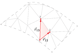
Figure S6: Triangular mesh showing the vector definitions for a single triangle.

From Eqs. (S17) and (S21) is easy to see that it is more convenient to express stretching energy in terms of the distance between vertices of one triangle, $\mathbf{r}_{ij}$ ($\mathbf{r}_{12},\mathbf{r}_{13}$) (Fig. S6). Thus, using the chain rule we can write the force over the triangle vertices as,

$$\mathbf{f}_{i}=-\left(\partial_{\mathbf{r}_{ij}}E_{s}\right)\left(\frac{\partial\mathbf{r}_{ij}}{\partial\mathbf{r}_{i}}\right).$$ (S23)

After lengthy but straightforward algebra, the expression for the force on vertex $i$ due to stretching reads,

$$\begin{split}\mathbf{f}_{i}=&-\left[\frac{A_{T}Yh}{4\left(1-\nu^{2}\right)}\left[\left(F_{11}+\nu F_{22}\right)\begin{pmatrix}2\alpha_{11}\mathbf{r}_{12}+\alpha_{12}\mathbf{r}_{13}&\alpha_{12}\mathbf{r}_{12}\end{pmatrix}\right.\right.\\ +&\left(F_{22}+\nu F_{11}\right)\begin{pmatrix}\alpha_{12}\mathbf{r}_{13}&2\alpha_{22}\mathbf{r}_{13}+\alpha_{12}\mathbf{r}_{12}\end{pmatrix}\\ +&\left.(1-\nu)\left(F_{21}\begin{pmatrix}\alpha_{11}\mathbf{r}_{13}&2\alpha_{12}\mathbf{r}_{13}+\alpha_{11}\mathbf{r}_{12}\end{pmatrix}+F_{12}\begin{pmatrix}2\alpha_{12}\mathbf{r}_{12}+\alpha_{22}\mathbf{r}_{13}&\alpha_{22}\mathbf{r}_{12}\end{pmatrix}\right)\right]\\ +&\left.\frac{e_{s}}{4A_{T}}\begin{pmatrix}g_{22}\mathbf{r}_{12}-g_{12}\mathbf{r}_{13}&g_{11}\mathbf{r}_{13}-g_{12}\mathbf{r}_{12}\end{pmatrix}\right]\begin{pmatrix}-1&1&0\\ -1&0&1\end{pmatrix},\end{split}$$ (S24)

where $\alpha_{ij}=\left(\bar{g}^{-1}\right)_{ij}$. This expression can be directly implemented in a simulation.

IV.2 Bending energy

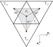
Figure S7: A triangle $T_{i}$ and three of its nearest neighbours $T_{j}$. In the continuum limit $b\to 0$. Shaded are is the vertex area element.

In order to derive expressions of the discrete version of the bending energy we start from Eq. (S13) and use the fact that $\kappa_{G}=-\kappa\left(1-\nu\right)$ to obtain

$$\begin{split}E_{bend}&=2\kappa H^{2}+\kappa_{G}K\\ &=\kappa\left(2H^{2}-K\right)+\nu\kappa K.\end{split}$$ (S25)

We can now use, $\mathrm{Tr}\left[\left(b_{\mu}^{\gamma}\right)^{2}\right]=4H^{2}-2K$ to write

$$\begin{split}E_{bend}&=\frac{1}{2}\kappa\mathrm{Tr}\left[\left(b_{\alpha}^{\beta}\right)^{2}\right]+\nu\kappa K\\ &=\frac{1}{2}\kappa g^{\beta\gamma}g^{\alpha\delta}b_{\alpha\gamma}b_{\beta\delta}+\nu\kappa K.\end{split}$$

If we use the definition of the second fundamental form we obtain

$$\begin{split}E_{bend}&=\frac{1}{2}\kappa g^{\beta\gamma}g^{\alpha\delta}\mathbf{e}_{\alpha}\cdot\partial_{\gamma}\mathbf{n}\mathbf{e}_{\beta}\cdot\partial_{\delta}\mathbf{n}+\nu\kappa K\\ &=\frac{1}{2}\kappa g^{\beta\gamma}\delta_{\beta}^{\delta}\partial_{\gamma}\mathbf{n}\cdot\partial_{\delta}\mathbf{n}+\nu\kappa K\\ &=\frac{1}{2}\kappa\partial_{\gamma}\mathbf{n}\cdot\partial^{\gamma}\mathbf{n}+\nu\kappa K.\end{split}$$

Following Ref. (Seung, ) the $\frac{1}{2}\kappa\partial_{\gamma}\mathbf{n}\cdot\partial^{\gamma}\mathbf{n}$ term is a continuum version of the expression

$$\begin{split}E_{SN}&=\frac{1}{2}\tilde{\kappa}\sum_{T_{j}.n.n.T_{i}}\left|\mathbf{n}_{T_{i}}-\mathbf{n}_{T_{j}}\right|^{2}\\ &\underbrace{=}_{\left\|\mathbf{n}\right\|=1}\tilde{\kappa}\sum_{T_{j}.n.n.T_{i}}\left(1-\mathbf{n}_{T_{i}}\cdot\mathbf{n}_{T_{j}}\right),\end{split}$$ (S26)

where $T_{i}$ is the triangle $i$, $T_{j}$ are three of its neighbours and $\tilde{\kappa}$ is the discrete value of the bending rigidity and subscript “SN” stands for “Seung-Nelson”. $\tilde{\kappa}$ is related proportional to $\kappa$ and we’ll discuss the constant of proportionality below. The sum in Eq. (S26) can be written as

$$\begin{split}E_{SN}&=\frac{1}{2}\tilde{\kappa}\sum_{j}\left|\mathbf{n}\left(\mathbf{r}_{i}\right)-\mathbf{n}\left(\mathbf{r}_{i}+b\mathbf{v}^{\left(j\right)}\right)\right|^{2},\end{split}$$

where $b$ is the distance between centers of two neighbouring triangles and vectors $\mathbf{v}$ are (see Fig. S7)

$$\mathbf{v}^{\left(j\right)}=\cos\left(\frac{2\pi}{3}j\right)\mathbf{e}_{x}+\sin\left(\frac{2\pi}{3}j\right)\mathbf{e}_{y}.$$

For $b\to 0$ we can use Taylor series to expand $\mathbf{n}\left(\mathbf{r}_{i}+b\mathbf{v}^{\left(j\right)}\right)$ to the linear order in $b$,

$$\mathbf{n}\left(\mathbf{r}_{i}+b\mathbf{v}^{\left(j\right)}\right)=\mathbf{n}\left(\mathbf{r}_{i}\right)+b\left.\partial^{\phi}\mathbf{n}\right|_{\mathbf{r}_{i}}v_{\phi}^{\left(j\right)}+o\left(b^{2}\right).$$ (S27)

Thus,

$$\begin{split}E_{SN}&=\frac{b^{2}}{2}\tilde{\kappa}\sum_{j}\left.\partial^{\phi}\mathbf{n}\right|_{\mathbf{r}_{i}}v_{\phi}^{\left(j\right)}\left.\partial_{\psi}\mathbf{n}\right|_{\mathbf{r}_{i}}v_{\left(j\right)}^{\psi}\\ &=\frac{b^{2}}{2}\tilde{\kappa}\left.\partial^{\phi}\mathbf{n}\right|_{\mathbf{r}_{i}}\left.\partial_{\psi}\mathbf{n}\right|_{\mathbf{r}_{i}}\sum_{j}v_{\phi}^{\left(j\right)}v_{\left(j\right)}^{\psi}.\end{split}$$

We can now calculate the $j$-sum explicitly for each component $\phi=x,y$ and $\psi=x,y$,

$$\begin{split}\sum_{j=1}^{3}v_{x}^{\left(j\right)}v_{\left(j\right)}^{x}&=\sum_{j=1}^{3}\cos^{2}\left(\frac{2\pi}{3}j\right)=\frac{3}{2}\\ \sum_{j=1}^{3}v_{y}^{\left(j\right)}v_{\left(j\right)}^{y}&=\sum_{j=1}^{3}\sin^{2}\left(\frac{2\pi}{3}j\right)=\frac{3}{2}\\ \sum_{j=1}^{3}v_{x}^{\left(j\right)}v_{\left(j\right)}^{y}&=\sum_{j=1}^{3}\sin\left(\frac{2\pi}{3}j\right)\cos\left(\frac{2\pi}{3}j\right)=0,\end{split}$$

and

$$E_{SN}=\frac{3}{2}\frac{b^{2}}{2}\tilde{\kappa}\partial^{\phi}\mathbf{n}\partial_{\phi}\mathbf{n},$$

and we assume that $\partial_{\phi}\mathbf{n}$ is calculated at point $\mathbf{r}_{i}$. We write $E_{SN}=-\frac{3}{2}\frac{b^{2}}{2}\tilde{\kappa}\partial^{\phi}\mathbf{n}b_{\phi}^{\mu}\mathbf{e}_{\mu}=\frac{3}{2}\frac{b^{2}}{2}\tilde{\kappa}\mathrm{Tr}\left(b_{\phi}^{\mu}\right)^{2}=\frac{3b^{2}}{4}\tilde{\kappa}\left(4H^{2}-2K\right)=\frac{3b^{2}}{2}\tilde{\kappa}\left(2H^{2}-K\right)$. Thus, the total discrete energy is

$$E_{SN}^{tot}=\frac{3}{2}\tilde{\kappa}\sum_{T_{i}}b^{2}\left(2H_{T_{i}}^{2}-K_{T_{i}}\right),$$

where $H_{T_{i}}$ and $K_{T_{i}}$ are mean and Gaussian curvature of the triangle $T_{i}$ and the sum goes over all triangles. From Fig. S7 we see that the area element $A_{i}=\frac{b^{2}\sqrt{3}}{2}$, which leads to

$$E_{SN}^{tot}=\frac{1}{\sqrt{3}}\tilde{\kappa}\sum_{T_{i}}A_{i}\left(2H_{T_{i}}^{2}-K_{T_{i}}\right),$$

which in the limit $A_{i}\to 0$ becomes an integral

$$E_{SN}^{tot}=\frac{1}{\sqrt{3}}\tilde{\kappa}\int_{A}\left(2H^{2}-K\right).$$

Comparing Eq. (S25) with the last expression we obtain $\kappa=\frac{1}{\sqrt{3}}\tilde{\kappa}$. Note that this is a different prefactor than obtained in Refs. (Seung, ) and (Schmidt, ). The reason is that in Eq. (S27) we have truncated the expansion to early. The exact constant of proportionality is of the same order of magnitude and is given as $\kappa=\frac{\sqrt{3}}{2}\tilde{\kappa}$ Therefore, we have showed that Eq. (S26) is a good discrete approximation for the continuum elastic energy. The advantage of the last expression is that it can be easily computed in a simulation.

IV.2.1 Vertex bending force

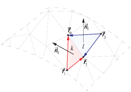
Figure S8: Edge $e$ shared by the faces $k$ and $l$ shown along with their associated normals.

The bending energy of a triangular mesh can be expressed as Eq. (S26),

$$E_{B}=\tilde{\kappa}\sum_{e\in\text{Edges}}\left(1-{\mathbf{n}}_{e,1}\cdot{\mathbf{n}}_{e,2}\right),$$ (S28)

where $e$ is an edge of the mesh and $\mathbf{n}_{e,1(2)}$ are the unit-length normals of two neighbouring triangles. For the shake of simplicity we consider a sole edge and two triangles $k$ and $l$ as is shown in Fig. S8. Note that $\mathbf{n}_{k(l)}=\mathbf{A}_{k(l)}/A_{k(l)}$, where $\mathbf{A}_{k(l)}$ is a vector normal to the triangle having length equal to the triangle’s area.

Now the bending force over a vertex $p$ is the negative gradient $E_{B}$ calculated at $\mathbf{r}_{p}$,

$$\begin{split}\mathbf{f}_{p,e}&=-\tilde{\kappa}\nabla_{\mathbf{r}_{p}}\sum_{e\epsilon Edges}\left(\frac{\mathbf{A}_{k}\cdot\mathbf{A}_{l}}{|\mathbf{A}_{k}|\,|\mathbf{A}_{l}|}\right)\\ &=-\tilde{\kappa}\nabla_{\mathbf{r}_{p}}\sum_{e\epsilon Edges}\mathbf{f}_{p,e},\end{split}$$ (S29)

is easy to see that since we are dealing with a sum over all the edges then it suffice to calculate the gradient $\nabla_{\mathbf{r}_{p}}$ for one generic edge,

$$\mathbf{f}_{p,e}=-\tilde{\kappa}\left(\partial_{\mathbf{r}_{ij}}E_{B,e}\right)\left(\frac{\partial\mathbf{r}_{ij}}{\partial\mathbf{r}_{p}}\right).$$ (S30)

After straightforward but lengthy algebra, the force matrix $\mathbf{f}_{p,e}$, Eq. (S30) is,

$$\mathbf{f}_{p,e}=-\tilde{\kappa}\left(\partial_{\mathbf{r}_{ij}}E_{B,e}\right)\begin{pmatrix}-1&1&0&0\\ -1&0&1&0\\ -1&0&0&1\end{pmatrix},$$ (S31)

with

$$\begin{split}\left(\partial_{\mathbf{r}_{ij}}E_{B,e}\right)=&\partial_{\mathbf{r}_{ij}}\left(\frac{\mathbf{A}_{k}\cdot\mathbf{A}_{l}}{|\mathbf{A}_{k}|\,|\mathbf{A}_{l}|}\right)\\ =&\frac{1}{|\mathbf{A}_{k}|\,|\mathbf{A}_{l}|}\left[\partial_{\mathbf{r}_{ij}}\left(\mathbf{A}_{k}\cdot\mathbf{A}_{l}\right)-\left(\mathbf{A}_{k}\cdot\mathbf{A}_{l}\right)\left(\frac{1}{|\mathbf{A}_{k}|}\partial_{\mathbf{r}_{ij}}|\mathbf{A}_{k}|+\frac{1}{|\mathbf{A}_{l}|}\partial_{\mathbf{r}_{ij}}|\mathbf{A}_{l}|\right)\right]\\ =&\frac{1}{4|\mathbf{A}_{k}|\,|\mathbf{A}_{l}|}\left[\begin{array}[]{c}\\ \\ \end{array}\right.\\ &\left(\left(\mathbf{r}_{02}\cdot\mathbf{r}_{03}\right)\mathbf{r}_{02}-\left(\mathbf{r}_{02}\cdot\mathbf{r}_{02}\right)\mathbf{r}_{03}\left(\mathbf{r}_{02}\cdot\mathbf{r}_{03}\right)\mathbf{r}_{01}\right.\\ &+\left(\mathbf{r}_{01}\cdot\mathbf{r}_{02}\right)\mathbf{r}_{03}-2\left(\mathbf{r}_{01}\cdot\mathbf{r}_{03}\right)\mathbf{r}_{02}\left(\mathbf{r}_{01}\cdot\mathbf{r}_{02}\right)\mathbf{r}_{02}\\ &-\left.\left(\mathbf{r}_{02}\cdot\mathbf{r}_{02}\right)\mathbf{r}_{01}\right)\\ +&\left(\mathbf{A}_{k}\cdot\mathbf{A}_{l}\right)\left(\frac{1}{|\mathbf{A}_{k}|^{2}}\begin{pmatrix}\left(\mathbf{r}_{02}\cdot\mathbf{r}_{02}\right)\mathbf{r}_{01}-\left(\mathbf{r}_{01}\cdot\mathbf{r}_{02}\right)\mathbf{r}_{02}&\left(\mathbf{r}_{01}\cdot\mathbf{r}_{01}\right)\mathbf{r}_{02}-\left(\mathbf{r}_{01}\cdot\mathbf{r}_{02}\right)\mathbf{r}_{01}&0\end{pmatrix}\right.\\ +&\left.\left.\frac{1}{|\mathbf{A}_{l}|^{2}}\begin{pmatrix}0&\left(\mathbf{r}_{03}\cdot\mathbf{r}_{03}\right)\mathbf{r}_{02}-\left(\mathbf{r}_{02}\cdot\mathbf{r}_{03}\right)\mathbf{r}_{03}&\left(\mathbf{r}_{02}\cdot\mathbf{r}_{02}\right)\mathbf{r}_{03}-\left(\mathbf{r}_{02}\cdot\mathbf{r}_{03}\right)\mathbf{r}_{02}\end{pmatrix}\right)\right].\end{split}$$ (S32)

V Active Remodelling

Remodelling is introduced as a change in the local reference metric $\bar{g}$. Here we choose a circular geometry for which we have the following natural metric (Fig. S9),

$$\bar{g}_{ij}(\{r,\theta\},t)=\left(\begin{array}[]{cc}g_{11}(\{r,\theta\},t)&g_{12}(\{r,\theta\},t)\\ g_{12}(\{r,\theta\},t)&g_{22}(\{r,\theta\},t)\end{array}\right),$$ (S33)

and for simplicity we impose a non-shear linear uniform remodelling, i.e.,

$$\begin{split}\partial_{t}g_{11}(\{r,\theta\},t)&=\beta_{11}\\ \partial_{t}g_{12}(\{r,\theta\},t)&=\frac{1}{2}\left[\left(\frac{g_{22}}{g_{11}}\right)^{\frac{1}{2}}\beta_{11}+\left(\frac{g_{11}}{g_{22}}\right)^{\frac{1}{2}}\beta_{22}\right]\cos\phi\\ \partial_{t}g_{22}(\{r,\theta\},t)&=\beta_{22},\end{split}$$ (S34)

with $\beta_{11}$ and $\beta_{22}$ being the remodelling rates in the $\mathbf{R}_{12}$ and $\mathbf{R}_{13}$ direction and $\phi$ is the angle between $\mathbf{R}_{12}$ and $\mathbf{R}_{13}$. Eqs. (S33) and (S34) can be easily discretised by expressing the metric tensor in the triangle laboratory coordinates.

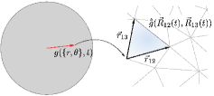
Figure S9: Active remodelling is introduced as a change of the reference metric of each triangle.

VI Viscoelastic relaxation

As in Ref. Muoz we model viscoelastic dissipation via an internal rearrangement processes leading to the relaxation of the reference metric towards the realised (i.e., current) metric, i.e.,

$$\partial_{t}{\bar{g}_{ij}}=\frac{1}{\tau_{ve}}\left(g_{ij}-\bar{g}_{ij}\right),$$ (S35)

where ${g}_{ij}$, $\bar{g}_{ij}$ are the current and reference metric tensors at time $t$, respectively, and $\tau_{ve}$ is the remodelling time scale. The physical interpretation of Eq. (S35) is that the energy is dissipated in local rearrangement processes.

VII Numerical implementation

We have built our own parallel GPU-based (NVidia CUDA) implementation of the discrete model outlined in the previous sections. Our code is specifically designed to introduce different sources of activity into the system. The general workflow is shown in Fig. S10. All computation-heavy task are fully implemented on the GPU, so that there are no transfers between DEVICE-HOST during the execution. The only routines executed by the host are those required by the user in order to save data.

Our CUDA kernels are moderately optimized, trying to keep aligned and coalesced memory access avoiding threads divergence and only using atomic functions when absolutely necessary. Finally, we used ParaView paraview as an external visualisation software for testing and presentation purposes.

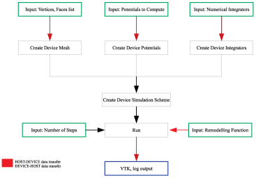
Figure S10: Schematic diagram of the software implementation.

VII.1 Simulation parameters

The coarse-grained triangular meshes used in the simulation were created using a public domain package Gmsh (gmesh, ) setting the edge target length to $l=0.35$ and the plate radius equal to $R=50$, with all lengths measured in units of thickness, $h$. In order to obtain different initial configuration the vertices are moved randomly in $(x,y)$ around the initial configuration using a normal distribution with standard deviation equal to $10^{-3}$. After this procedure the Device Mesh is created and the reference metric is set to the mesh actual metric.

The potentials used in our simulation with its respective parameters are listed in Table 1. It is important to note that all material parameter are assumed to be time-independent and uniform across the entire mesh.

Streaching Potential	Value
Young’s modulus, $E$	$10^{2}$
Plate thickness, $h$	$10^{0}$
Poissson’s ratio, $\nu$	$1/3$
Seung-Nelson Bending Potential
Bending modulus, $\kappa$	$5\times 10^{-2}(E\,h^{3})$

Table 1: Simulation parameters.

The active remodelling processes are assumed not to be uniform on the mesh. In particular, we have chosen to restrict remodelling and remodelling to an external annulus of $20<r<50$. The remodelling and viscous remodelling rate are set to be uniform inside of the annulus, for the respective values used in the simulation, see Fig. 3.

To integrate the vertex equation of motion, we have implemented a Brownian dynamics integrator,

$$\partial_{t}\mathbf{r}_{i}=\mu\mathbf{F}_{i}+\mathbf{F}_{R},$$

where $\mu$ is the inverse friction coefficient and $\mathbf{F}_{i}$ is the total force acting on the vertex $i$ due the mesh deformation and $\mathbf{F}_{R}$ is a uniform random force whose magnitude fullfil the fluctuation-dissipation theorem for the given inverse friction coefficient and temperature, $T$; in our simulation we set $\mu=1.0$ and $T=10^{-6}$. In addition, the integration is set to be $10^{-3}$ for remodelling rates equal or smaller than $10^{-3}$ and $10^{-5}$ otherwise.

VIII Elastic relaxation time

Here we make a rough estimate of the elastic relaxation time scale assuming that the a nearly flat sheet is suspended in a fluid. We assume that the fluid only provides drag and do not consider any effects of its flow, i.e., the fluid acts as a simple sink for the sheet’s momentum. Assuming only out of plane motion described by the high function $w(x,y)$, in the overdamped limit the equation of motion is,

$$\Gamma\partial_{t}w=\kappa\Delta^{2}w,$$

where $\Delta^{2}$ is the bi-laplacian operator and $\Gamma$ is the friction coefficient due to fluid. Note that $\Gamma$ has dimensions of $\frac{\text{mass}}{\text{length}^{2}\times\text{time}}$, and is thus interpreted as the friction per unit area. If we recall the well-known result in fluid dynamics (Lamb, ) that the drag coefficient on a disk of radius $R$ moving perpendicular to its plane in a fluid of viscoelastic $\eta$ is $\zeta=16\eta Rv$, where $v$ is the velocity, we obtain $\Gamma=\frac{16}{\pi}\frac{\eta v}{R}$. Therefore, we estimate

$$\Gamma\frac{h}{\tau_{el}}=\kappa\frac{h}{R^{4}},$$

or

$$\tau_{el}=\frac{16}{\pi}\frac{\eta R^{3}}{\kappa}.$$

For an epithelial tissue of size $R\sim 1$ mm in water, assuming bending rigidity $\kappa\sim 10^{-12}$ J, we estimate $\tau_{el}\sim 10$ s.

References

Thompson (1942)D. W. Thompson, On Growth and Form (Cambridge Univ. Press, 1942).
Alberts et al. (2014)B. Alberts, A. Johnson,
J. Lewis, M. Raff, K. Roberts, and P. Walter, Molecular Biology of the Cell, 6th ed. (Garland Science, New York, 2014).
Wolpert et al. (2015)L. Wolpert, C. Tickle, and A. M. Arias, Principles of Development (Oxford University Press, USA, 2015).
Marchetti et al. (2013)M. C. Marchetti, J.-F. Joanny, S. Ramaswamy,
T. B. Liverpool, J. Prost, M. Rao, and R. A. Simha, Rev. Mod. Phys. 85, 1143 (2013).
Harris et al. (2012)A. R. Harris, L. Peter,
J. Bellis, B. Baum, A. J. Kabla, and G. T. Charras, Proc. Natl. Acad. Sci. 109, 16449 (2012).
Berthoumieux et al. (2014)H. Berthoumieux, J.-L. Maître, C.-P. Heisenberg, E. K. Paluch, F. Jülicher, and G. Salbreux, New
J. Phys. 16, 065005
(2014).
Matoz-Fernandez et al. (2017)D. Matoz-Fernandez, E. Agoritsas, J.-L. Barrat, E. Bertin, and K. Martens, Phys. Rev. Lett. 118, 158105 (2017).
Henkes et al. (2011)S. Henkes, Y. Fily, and M. C. Marchetti, Phys. Rev. E 84, 84 (2011).
Berthier and Kurchan (2013)L. Berthier and J. Kurchan, Nat.
Phys. 9, 310 (2013).
Petitjean et al. (2010)L. Petitjean, M. Reffay,
E. Grasland-Mongrain,
M. Poujade, B. Ladoux, A. Buguin, and P. Silberzan, Biophys. J. 98, 1790 (2010).
Angelini et al. (2011)T. E. Angelini, E. Hannezo,
X. Trepat, M. Marquez, J. J. Fredberg, and D. A. Weitz, Proc. Natl. Acad. Sci. USA 108, 4714 (2011).
Chepizhko et al. (2018)O. Chepizhko, M. C. Lionetti, C. Malinverno, C. Giampietro, G. Scita,
S. Zapperi, and C. A. La Porta, Soft Matter 14, 3774 (2018).
Henkes et al. (2019)S. Henkes, K. Kostanjevec,
J. M. Collinson, R. Sknepnek, and E. Bertin, arXiv preprint arXiv:1901.04763 (2019).
Salbreux and Jülicher (2017)G. Salbreux and F. Jülicher, Phys. Rev. E 96, 032404
(2017).
Efrati et al. (2009)E. Efrati, E. Sharon, and R. Kupferman, J. Mech. Phys.
Solids 57, 762 (2009).
Kang et al. (2014)S. H. Kang, S. Shan, A. Košmrlj, W. L. Noorduin, S. Shian, J. C. Weaver, D. R. Clarke, and K. Bertoldi, Phys. Rev. Lett. 112, 098701 (2014).
Clément et al. (2017)R. Clément, B. Dehapiot, C. Collinet,
T. Lecuit, and P.-F. Lenne, Curr. Biol. 27, 3132 (2017).
Audoly and Pomeau (2010)B. Audoly and Y. Pomeau, Elasticity and Geometry
- From Hair Curls to the Non-linear Response of Shells (Oxford University Press, Oxford, UK, 2010).
Do Carmo (1976)M. Do Carmo, Differential Geometry
of Curves and Surfaces, Vol. 1 (Prentice-Hall Englewood Cliffs, NJ, 1976).
Koiter (1966)W. Koiter, Koninklijke Nederlandse Akademie van Wetenschappen, Proceedings, Series B 69, 1 (1966).
(21)Supplemental Material available at:
xxxxxxx.
Marmottant et al. (2009)P. Marmottant, A. Mgharbel, J. Käfer,
B. Audren, J.-P. Rieu, J.-C. Vial, B. Van Der Sanden, A. F. Marée, F. Graner, and H. Delanoë-Ayari, Proc. Natl. Acad. Sci. 106, 17271 (2009).
Joanny and Prost (2009)J.-F. Joanny and J. Prost, HFSP J. 3, 94 (2009).
Rauzi et al. (2008)M. Rauzi, P. Verant,
T. Lecuit, and P.-F. Lenne, Nat. Cell Biol. 10, 1401 (2008).
Rauzi et al. (2010)M. Rauzi, P.-F. Lenne, and T. Lecuit, Nature 468, 1110 (2010).
Sknepnek and Olvera de la
Cruz (2012)R. Sknepnek and M. Olvera
de la Cruz, Phys. Rev. E 85, 050501
(2012).
Jagla (2007)E. Jagla, Phys.
Rev. B 75, 085405
(2007).
Davidovitch et al. (2011)B. Davidovitch, R. D. Schroll, D. Vella,
M. Adda-Bedia, and E. A. Cerda, Proc. Natl. Acad. Sci. 108, 18227 (2011).
Amar and Wu (2014)M. B. Amar and M. Wu, EPL (Europhysics
Letters) 108, 38003
(2014).
Yan et al. (2019)J. Yan, C. Fei, S. Mao, A. Moreau, N. S. Wingreen, A. Košmrlj, H. A. Stone, and B. L. Bassler, eLife 8, e43920 (2019).
Goriely (2017)A. Goriely, The Mathematics And
Mechanics Of Biological Growth, Vol. 45 (Springer, 2017).
Amar and Goriely (2005)M. B. Amar and A. Goriely, J. Mech. Phys.
Solids 53, 2284
(2005).
Goriely and Amar (2005)A. Goriely and M. B. Amar, Phys.
Rev. Lett. 94, 198103
(2005).
Goriely and Amar (2007)A. Goriely and M. B. Amar, Biomech.
Model. Mechanobiol. 6, 289 (2007).
Rodriguez et al. (1994)E. K. Rodriguez, A. Hoger, and A. D. McCulloch, J. Biomech. 27, 455 (1994).
Ruiz-Herrero et al. (2019)T. Ruiz-Herrero, T. G. Fai, and L. Mahadevan, arXiv preprint arXiv:1901.04406 (2019).

References

(1)A. E. Green and W. Zerna, Theoretical Elasticity,
2nd edition, Dover Publications, 1992.
(2)W. T. Koiter, On the Non-linear Theory of Thin Elastic
Shells, Proceedings, Series B, Physical Sciences, Amsterdam 1951.
(3)E. Efrati, E. Sharon, and R. Kupferman, Elastic theory
of unconstrained non-Euclidean plates, J. Mech. Phys. Solid., 57,
762 (2009).
(4)W. T. Koiter, A Consistent First Approximation in
the General Theory of Thin Elastic Shells, Proc. IUTAM, Delft (1959).
(5)M. P. do Carmo, Differential Geometry of Curves
and Surfaces, Prentice Hall, 1976.
(6)H. S. Seung and D. R. Nelson, Defects in flexible
membranes with crystalline order, Phys. Rev. A, 38, 1005 (1988).
(7)M. Parrinello and A. Rahman, Polymorphic transitions
in single crystals: A new molecular dynamics method, J. Appl. Phys.
52, 7182 (1981).
(9)B. Schmidt and F. Fraternali, Universal formulae
for the limiting elastic energy of membrane networks, Journal of the
Mechanics and Physics of Solids 60.1, 172-180 (2012).
(10) Muñoz, José J., and Santiago Albo,
Physiology-based model of cell viscoelasticity.
Physical Review E 88.1 (2013): 012708.
(11) C. Geuzaine and J.-F. Remacle. Gmsh: a three-dimensional
finite element mesh generator with built-in pre- and post-processing
facilities. International Journal for Numerical Methods in Engineering
79(11), pp. 1309-1331, 2009 (http://gmsh.info/).
(12) H. Lamb, Hydrodynamics, 6th edition, Cambridge University Press.
(13) Ahrens, James, Geveci, Berk, Law, Charles, ParaView: An End-User Tool for Large Data Visualization, Visualization Handbook, Elsevier, 2005.