A joint deconvolution algorithm to combine single dish and interferometer data for wideband multi-term and mosaic imaging

Abstract

Imaging in radio astronomy is usually carried out with a single-dish radio telescope doing a raster scan of a region of the sky or with an interferometer that samples the visibility function of the sky brightness. Mosaic observations are the current standard for imaging large fields of view with an interferometer and multi-frequency observations are now routinely carried out with both types of telescopes to increase the continuum imaging sensitivity and to probe spectral structure. This paper describes an algorithm to combine wideband data from these two types of telescopes in a joint iterative reconstruction scheme that can be applied to spectral cube or wideband multi-term imaging both for narrow fields of view as well as mosaics. Our results demonstrate the ability to prevent instabilities and error that typically arise when wide-band or joint mosaicing algorithms are presented with spatial and spectral structure that is inadequetely sampled by the interferometer alone. For comparable noise levels in the single dish and interferometer data, the numerical behaviour of this algorithm is expected to be similar to the idea of generating artificial visibilities from single dish data. However, our discussed implementation is simpler and more flexible in terms of applying relative data weighting schemes to match noise levels while preserving flux accuracy, fits within standard iterative image reconstruction frameworks, is fully compatible with wide-field and joint mosaicing gridding algorithms that apply corrections specific to the interferometer data and may be configured to enable spectral cube and wideband multi-term deconvolution for single-dish data alone.

1 Introduction

The combination of images and data from single dish telescopes and radio interferometers has been a topic of interest for many years. A single-dish radio telescope forms an image by doing a raster scan of a region of the sky and the observed image can be described as a convolution of the true sky with an effective single dish beam pattern. An interferometric array samples the visibility function of the sky brightness distribution over a region of sky covered by the forward gain pattern of each array element and forms an image by Fourier inversion and iterative model reconstruction. A processed interferometric image represents a convolution of the true sky with a Gaussian corresponding to the main lobe of the interferometer impulse response function. At a given observing frequency, a radio interferometer usually offers excellent angular resolution compared to a single dish telescope, but it suffers from the short-spacing problem where the total power and visibility function for sources with large angular size and low surface brightness are often not measured at all or well enough for an accurate reconstruction. This is especially relevant for mosaic observations of large fields of view containing spatial structure that extends beyond the field of view offered by each individual pointing.

With the widespread adoption of wideband recievers on both types of radio telescopes, wideband imaging techniques are now used to combine data across a large range of observing frequencies. The main purpose is to increase imaging sensitivity and fidelity as well as to reconstruct both the spatial and spectral structure of the sky brightness distribution. Using joint reconstruction algorithms such as MTMFS (Rau & Cornwell, 2011; Sault & Wieringa, 1994), reconstructions of both intensity and spectral structure can be done at an angular resolution offered by the joint spatial frequency coverage and not limited to the angular resolution offered by the lowest frequency. So far, this technique has been applied only to wideband interferometer data although there is nothing conceptual preventing it from being used on wideband single dish data as well.

With wideband interferometer data alone, a reconstruction of spectral structure at the largest spatial scales is completely unconstrained by the data. A subtle difference with intensity-only imaging is that the problem exists even for situations where they may be enough data for an adequate reconstruction of large scale intensity. As shown in an example in Rau & Cornwell (2011), there may be no apparent imaging artifacts as the model adequately fits the measured data, but the spectral reconstruction will still be wrong.

Over the years, several approaches have been tried and used, with varying degrees of success. They range from combining fully processed images from single dish and interferometry data, to using the single dish image as a starting model for the interferometer reconstruction and finally to various schemes for joint reconstructions of the sky model using constraints from both datasets at once. It has been shown that best results are obtained when the iteratively reconstructed model represents the entire structure on the sky and not just some spatial scales.

This paper formulates a joint reconstruction algorithm that always uses constraints from both sets of data and follows the standard major/minor cycle approach to iterative image reconstruction in radio interferometry. The algorithm can be configured for spectral cube imaging as well as wide-band multi-term imaging and is fully compatible with wide-field interferometric imaging schemes such as AW-Projection (Bhatnagar et al., 2008) and Joint Mosaicing (Sault et al., 1996). It can also be configured to provide spectral cube and wideband multi-term deconvolution of the single dish data alone and these deconvolved single dish models can in turn be used in traditional feathering and startmodel approaches.

Sections 2 and 3 summarize wideband imaging with a single dish and interferometer respectively and section 4 summarizes existing combination approaches. Section 5 describes our algorithm with imaging results presented in section 6.

2 Single Dish imaging

A single dish radio telescope makes an image of the sky by doing a raster scan across the region of interest, a process often refered to as basket-weaving. This is mathematically equivalent to a convolution of the true sky image $I^{sky}$ with the antenna power pattern. An image is then constructed by resampling the measurements onto an image pixel grid using an explicit gridding kernel to compute a weighted average of all data points within the support radius around each pixel center.

The observed image $I^{obs}_{SD,\nu}$ can be represented as

$$I^{obs}_{SD,\nu}=I^{sky}_{\nu}\star I^{psf}_{SD,\nu}$$ (1)

where $I^{psf}_{SD,\nu}=I^{PB}_{SD,\nu}\star I^{grid}_{SD}$ is an aggregate convolution function constructed from the antenna power pattern and the image gridding kernel. The angular resolution of the observed image is given by $\theta_{SD,\nu}=\sqrt{\left[\theta_{PB,\nu}^{2}+\theta_{grid}^{2}\right]}$ where $\theta_{PB,\nu}=\frac{\lambda}{D}$ is the half-power beam width of the SD primary and $\theta_{grid}$ is the width of the image gridding kernel. In the limit of very fine sampling on the sky as well as on the image grid, the sky and pixel sampling patterns may be ignored in this analysis. At an observing frequency $\lambda$, a single dish telescope is sensitive to spatial frequencies ranging from zero to $\theta_{PB,\nu}=\frac{\lambda}{D}$ where $D$ is the effective diameter of the aperture and $\lambda$ is the observing wavelength. Wide band single dish observations will result in images at angular resolutions ranging from $\frac{\lambda_{max}}{D}$ to $\frac{\lambda_{min}}{D}$.

Mangum et al. (2007) formally describe the process of constructing a single dish image and choosing appropriate image gridding kernels and this is currently the approach used for ALMA total power data. Within the CASA software, wideband single dish data are usually imaged in spectral line mode, using a fixed image gridding kernel for all frequencies. For continuum imaging, data from multiple observing frequencies are combined onto a single output image grid, also using the same gridding kernel.

3 Interferometric imaging

An interferometer constructs an image by partially sampling the visibility function of the target sky brightness distribution. Measured visibilities are resampled onto a 2D spatial frequency grid by a process of convolutional resampling (called gridding) and then Fourier transformed to form the observed image.

The observed image $I^{obs}_{INT,\nu}$ can be approximately represented as

$$I^{obs}_{INT,\nu}=\left[I^{sky}_{\nu}\cdot{P_{\nu}}\right]\star I^{psf}_{INT,\nu}$$ (2)

where $I^{psf}_{INT,\nu}=[F]^{-1}S_{\nu}$ is the point spread function given by the inverse Fourier transform of the weighted 2D spatial frequency sampling functions at the observing frequency $\nu$ and ${P_{\nu}}$ is the primary beam (baseline power pattern) of each array element. The angular resolution of an interferometer (and typically also the image reconstructed from it) is therefore given by $\theta_{INT,\nu}=\lambda/B_{max}$.

A model of the true sky $I^{sky}_{model}$ is computed via an iterative image reconstruction scheme that uses a-priori information about the types of structures being imaged to estimate the visibility function in regions of the spatial frequency plane that the interferometer has not made measurements. Algorithms such as classic CLEAN (Högbom, 1974; Clark, 1980) model the sky as a series of delta functions, MS-CLEAN(Cornwell, 2008) uses a basis of inverted truncated paraboloids of specific widths, MT-MFS(Rau & Cornwell, 2011) uses a Taylor polynomial model to describe the frequency dependent amplitude per multi-scale flux component. Wide-field baseline-based effects due to array non-coplanarity (the W-term) and variable antenna primary beams are handled via the W-Projection (Cornwell et al., 2008) and A-Projection (Bhatnagar et al., 2008) that use careful choices of gridding convolution functions during interferometric imaging. Joint mosaic imaging (Sault et al., 1996) is performed (also often during gridding) as an appropriately weighted sum of data from a series of shifted pointings.

At a given observing frequency $\lambda$, an interferometer is sensitive to a finite set of spatial scales within the limits of $\lambda/B_{min}$ and $\lambda/B_{max}$ where $B_{min}$ and $B_{max}$ are the shortest and longest baselines that are possible for a given array configuration. The angular resolution of the reconstructed image is therefore given by $\lambda/B_{max}$. The maximum spatial scale that can be measured is $\theta_{INT}=\lambda/B_{min}$ where $B_{min}>D$ and it is left to the reconstruction process to estimate the visibility function at these and larger scales. The result therefore depends strongly on the accuracy and flexibility of the models used and this uncertainty is known as the short spacing problem. A negative bowl in the reconstructed image implies that large scales are missing from the reconstructed model. Other large scale artifacts could result when the reconstruction attempts to construct a model that spans the unmeasured large scales but fails to produce something physically plausible. Finally, with the use of multi-scale algorithms it is sometimes possible to produce images with artifact-free large-scale reconstructions but without external or a-priori information, one can never be sure that it is flux-accurate.

Interferometric mosaicing is often employed to cover fields of view much larger than the primary beam of each array element. Here, the short spacing problem becomes especially relevant when the sky emission has structure on scales larger than the single pointing field of view.

With wide-band observations, the frequency dependence of the instrument and the sky must also be taken into account during the reconstruction process. One option is to make a spectral cube, with varying angular resolution and sensitivity to large spatial scales. Another is the MTMFS algorithm and related approaches that solve for joint wideband models to produce maps of intensity as well as spectral structure at a resolution given by the combined beam. Additionally, for wide-field and mosaic imaging, frequency dependent antenna primary beams introduce an artificial spectral index into the wideband sky flux model. Post-deconvolution wideband beam correction eliminates it from the wideband model but methods also exist to remove it prior to the iterative deconvolution and model generation on a per antenna or timestep basis (Bhatnagar et al., 2013).

The short spacing problem for wideband imaging is slightly different from that of narrow-band imaging. The extent of the central unsampled region on the spatial frequency plane increases with observing frequency. There is a range of scales that are measured adequately enough for an accurate reconstruction at lower frequencies but which are completely missing at the higher end of the band, thus causing spectral structure to be completely unconstrained by the data. Most plausible wideband sky models will not be able to distinguish between this missing data and (for example) a genuine steep spectrum extended source.

As seen in the illustration in Fig.1, compact sources have a signature all across the uv-plane and therefore their spectra are well constrained, even at the full angular resolution. The spectral structure of extended emission, however, is particularly poorly sampled and therefore extremely error prone, even in situations where some frequencies do measure the visibility function adequately enough to reconstruct an accurate average intensity. Symptoms of this effect may include the typical negative bowl in the intensity image but it is also possible to obtain a perfectly legitimate-looking intensity pattern with an overly steep spectral reconstruction.

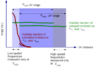
Figure 1: This diagram illustrates the spatial scales measured by an interferometer at different observing frequencies and its impact on the visibility function of a compact source as well as extended structure. The shaded rectangles represent the uv-range at the low and high frequency ends of an observing band. The green curve represents the measured visibility function of a point source with a negative spectral index, as measured at the low and high frequencies. The red curves represent the measured visibility function of an extended source, also with a negative spectral index. This figure illustrates the source of reconstruction uncertainty for extended sources, especially for spectral structure.

4 Combining single dish and interferometer data and images

Sections 4.1,4.2 and 4.3 summarize several techniques that have been in use for narrow-band imaging, discuss their strengths and weaknesses and explore their compatibility with wideband imaging. Section 4.4 lists the general approach followed by all the methods when dealing with interferometer primary beams for full-beam or mosaic imaging.

4.1 Feathering

Feathering is the technique most often used to combine images from single-dish instruments and interferometers. A composite image is obtained by computing a weighted sum of the observed single dish image and the reconstructed interferometer image, calculated in the spatial frequency domain. There are many variants of this approach, depending on weighting function choice and scale factors (for example, CASA feather(CASA_Docs, 2017), IMMERGE(MIRIAD_Docs, 2013),IMERG (AIPS_Docs, 2017), ObitFeather(Cotton, 2017)).

CASA feather implements the following.

$$\mathcal{F}(\textbf{I}^{feathered})={w_{sd}}{V_{sd}}+[1-{w_{sd}}]{V_{int}}$$ (3)

where ${w_{sd}}{V_{sd}}$ is the Fourier transform of the observed single-dish image given by Eqn. 1 and ${V_{int}}$ is the Fourier transform of the reconstructed interferometer image defined at a resolution given by the restoring beam. The single dish image is first scaled by the volume ratio of the interferometer restoring beam to the single dish antenna pattern. Then the weighting function is computed as

$${w_{sd}}=\mathcal{F}{I_{sd}}^{psf}~{}~{}\mathrm{scaled~{}to}~{}~{}max({w_{sd}})=1.0$$ (4)

The weight given to the Fourier transform of the restored interferometer image is then $[1-{w_{sd}}]$. Such a combination has the effect of using only well trusted regions of the spatial frequency plane from both images and selecting only those scales that each instrument measures best. Generally, the single-dish image is also pre-scaled by an additional gain parameter meant to correct for residual flux calibration errors. This is typically chosen by manually matching the flux in the overlapping range of spatial frequency. The IMMERGE implementation (MIRIAD_Docs, 2013) solves for this automatically by matching visibility function shapes within a user-defined annulus in the uv-domain.

Feathering is most appropriate when there are no reconstruction artifacts at scales other than the largest ones in the interferometer-only reconstruction and noise levels between the two images are comparable such that the addition of the single dish image does not degrade the interferometric image. Feathering is a single step process whose results depend strongly on the single-dish gain parameter as well as the specific shape of the weighting function. When the noise levels between the single dish and interferometer images differ significantly, one must choose between preserving flux correctness and keeping the noise level in the combined image close to that of the interferometric image. A significant amount of art is often involved in carefully constructing non-standard weighting functions in order to achieve this (i.e. by changing the form of Eqn.4). Although this might suffice for specific source structures and known noise characteristics, it is not a viable generic approach. Additionally, when structure is present on intermediate scales, an interferometer-only wideband reconstruction can perform unconstrained extrapolations which burn in errors in the model that are beyond the spatial frequency range that will be replaced by the single dish image. In such cases, a post-deconvolution combination may not be able to achieve flux correctness on all scales.

In situations where feathering can work well, it can be directly extended to wideband image reconstructions as well. The output of the MT-MFS algorithm is a set of Taylor coefficients that represent the spectral structure of the sky brightness distribution. A similar set of coefficient images must first be constructed from the single dish data, and the images feathered together term by term before recomputing derived quantities such as spectral index and curvature.

4.2 Single Dish image as a starting model or prior

A single dish observed image can be used to derive a starting model for the interferometric reconstruction. This approach is effective only when there is considerable overlap in measured spatial frequencies between the single dish and interferometer data such that the input starting model already accounts for much of the shorter spacing interferometer data. When there isn’t much overlap it is unlikely to be any different from feathering as the single dish image will provide no extra constraints for the interferometer reconstructions. Techniques such as MEM (Cornwell & Evans, 1985) make use of a-priori information and a single dish image can be used as a prior such that the reconstruction is biased towards it.

In situations where this startmodel approach is effective, wideband single dish data (or image cubes) can also be deconvolved separately and then converted to a set of Taylor coefficient model images to be supplied as a starting model for a wideband interferometer reconstruction.

4.3 Joint reconstructions

The most successful and robust approach is a joint reconstruction by which a single sky model is constructed using data and constraints from both data sets at once. Several methods are summarized below.

4.3.1 Joint image-domain constraints

Image solvers that directly implement optimization algorithms may modify their objective functions to include constraints from single dish as well as interferometric data. For example, the MOSMEM (MIRIAD_Docs, 2013) task in MIRIAD employs an image-domain chi-square constraint with separate terms for the interferometer dirty image as well as the single dish image, and implements this within a Maximum Entropy reconstruction algorithm (Cornwell & Evans, 1985). This implementation includes the option of pre-scaling the single dish data, along with the ability to optionally auto-scale it to match visibility functions in an annulus on the uv-plane that matched the overlap region. Wright (2012) analyses the joint imaging problem for ALMA+ACA+TP and the tests demonstrate that such a joint reconstruction is clearly superior to the previous two methods. For wideband imaging, the MEM sky model would have to be augmented to support a wideband flux model, a detail currently not included in existing literature or software. Algorithms such as RESOLVE Junklewitz et al. (2016) that have a Bayesian formulation along with a built-in wideband sky model may be an effective alternative algorithm within which to include similar single dish constraints.

Stanimirovic et al. (1999) describes another approach in which dirty images and point spread functions from both the interferometer and single dish are combined to form a new pair of images to feed into a deconvolution algorithm. In this particular application, a single scaling multiplier is optionally applied during an image-domain combination step. Stanimirovic et al. (1999) make no mention of how to handle primary beams or to do wideband imaging, but this method can easily be extended on those axes.

Note that both of these methods (MIRIAD_Docs, 2013; Stanimirovic et al., 1999) have been described as purely image-domain deconvolution approaches without any feedback loop to the raw data themselves. However, it is trivial to place these methods within the standard major/minor cycle imaging framework (Schwab & Cotton, 1983; Rau et al., 2009) and treat them as minor cycle image-domain modeling algorithms. The only extra required step would be to implement suitable model-to-data tranforms for the single dish data. Our algorithm described in section 5 describes such a framework.

4.3.2 Creating visibilities from single dish data

Koda et al. (2011) and Kurono et al. (2009) perform joint reconstructions by creating aritificial visibilities from single dish data and then including them in interferometer reconstructions. The single dish image is first linearly deconvolved using an estimate of the aggregate single dish beam. A randomised visibility sampling distribution is generated to match the shape of the Fourier transform of the single dish beam (similar to Eqn. 4) so as to preserve information about the intrinsic resolution of the single dish observation. New visibilities are then generated by a de-gridding step. For a mosaic observation, Koda et al. (2011) generate single dish visibilities for each interferometer pointing so as to be consistent with pointing table metadata already present in the interferometer dataset and which standard algorithms for joint mosaicing require. tp2vis is a recently developed solution targeted towards narrow-band (spectral cube) joint reconstructions for ALMA.

Koda et al. (2011) describe this algorithm for narrow-band (or spectral cube) imaging but it is a generic approach that can easily be extended to wideband image reconstruction. Qualitatively, this approach achieves the same results as the joint reconstructions mentioned above, with the added advantage of being naturally usable in existing software that implements iterative image reconstruction with major and minor cycles. Two practical caveats are that any software implementation would require very carefully crafted meta-data to ensure that the artificially generated visibilities are treated appropriately when used with interferometry-specific imaging options such as W-Projection (Cornwell et al., 2008) or A-Projection (Bhatnagar et al., 2008) as they use instrument-specific gridding convolution functions. Finally, the relative scaling or weighting of single-dish and interferometer data has to be done external to the reconstruction process.

4.4 Handling primary beams

From the forms of Eqns. 1 and 2, it is clear that the interferometer primary beam $P_{\nu}$ must be taken into account carefully for any field of view that goes beyond the inner central region of the beam where it can be approximated as unity. Only in that inner region can both observed images be described as convolutions of the sky brightness with a point spread function, thus allowing a simple linear combination to be usable within standard deconvolution routines.

A reconstructed wide-field interferometric image typically represents $I_{\nu}P_{\nu}$ and this is known as a flat-noise normalization. Interferometric image reconstruction is usually done with a flat-noise normalization and so any combination with single dish images prior to or during the reconstruction will require that the single dish image be modified to mimic the field-of-view as seen by the interferometer. This can be done by first performing a linear deconvolution of the single dish image using a model of the single dish beam, multiplying the resulting image by the interferometer primary beam (single field or mosaic) and then re-convolving the result by the single dish beam. The resulting single dish image now also represents a convolution of $I^{sky}\cdot P_{nu}$ with a point spread function, similar to Eqn.2. Koda et al. (2011) and Kurono et al. (2009) also describe this as steps done prior to calculating artificial single dish visibilities.

Note that for the startmodel approach (Sec.4.2) the last re-convolution step must be left out as the sky model is usually devoid of any point spread function. Alternatively, a flat-sky combination may also be performed. by first dividing out a primary beam model from the (flat-noise) interferometer image before feathering it with the single dish image. Similarly, a flat-sky startmodel approach would only require the single dish data to be linearly deconvolved prior to its use within the reconstruction.

5 SDINT reconstruction

In this paper we present a generic joint reconstruction algorithm for single dish and interferometer data. It combines and extends several of the ideas summarized above, and demonstrates a solution to the wideband short-spacing problem described in section 3.

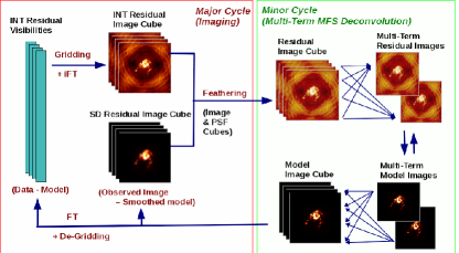
Figure 2: Joint reconstruction algorithm for wideband single dish and interferometer data. PSF and Residual image cubes from the interferometer and single dish data are combined prior to the minor cycle deconvolution step. This illustration emphasizes the ability to configure the algorithm to operate in spectral line mode as well as multi-term wideband continuum mode with either a point-source or multiscale sky model. The single dish data are represented as images but it is possible to include a data-image transform there as well.

A graphical representation of the basic algorithm is presented in Figure.2. Interferometer visibilities are gridded and imaged as a spectral cube and then combined with the single dish image cube. A similar combination is done with the interferometer point spread function and the representative single dish kernel ($I^{psf}_{SD,\nu}$ in Eq.1). The resulting pair of observed and PSF cubes are then sent to the minor cycle for image-plane deconvolution. Spectral cube deconvolution is performed directly with this new set of images and PSFs. Wideband multi-term deconvolution is performed by first constructing Taylor weighted averages across frequency to construct the set of inputs required by the MT-MFS algorithm. After a series of image-domain deconvolution iterations, the current model images are converted to model cubes (in the case of multi-term imaging) or used as is for spectral cube model prediction. Residuals are then computed for both the interferometer and the single dish data. For the interferometer data, it is the standard major cycle and for the single dish data a smoothed model is subtracted per channel from the observed single dish image cube. The new residuals are feathered together and the process repeats until an exit criterion is satisfied.

Pseudo-code listings based on the CASA PySynthesisImager tool (CASA_Docs, 2018) are provided in Algorithm.1 for joint spectral cube imaging and in Algorithm.2 for joint wideband multi-term imaging. The lines in black are the basic algorithm that follows Fig.2 and the lines in blue are steps required to include primary beams into the basic algorithm so that it may be applied to mosaic interferometer data. The recipes presented here assume a flat noise normalization of the interferometric gridder and minor cycle algorithm. Therefore, primary beams are divided out of the observed flat-noise image prior to feathering with the single dish data, and the result is re-multiplied by a primary beam to present a flat-noise input image to the minor cycle. For the wideband multi-term algorithm, an average or common primary beam is used in this second step in order to conform to the WBAWP algorithm (Bhatnagar et al. (2013)) that eliminates the primary beam frequency dependence prior to the multi-term minor cycle.

In this framework, spectral cube and multi-term deconvolution of the single dish data alone may also be done simply leaving out interferometer data and the feathering step. Examples from this algorithm configuration are included in the next section.

/* Initialize imagers and deconvolver */

IntCube = Imager(gridder=’interferometer’)

SDCube = Imager(gridder=’singledish’)

JointCube = Imager(deconvolver=’multiscale’)

/* Make PSFs */

IntCube.MakePSF()

SDCube.MakePSF()

JointCube.psf=Feather(IntCube.psf, SDCube.psf)

/* Make initial images */

IntCube.MakeRES()

SDCube.MakeRES()

IntCube.res = IntCube.res $\div$ IntCube.PB

JointCube.res=Feather(IntCube.res, SDCube.res)

JointCube.res = JointCube.res $\times$ IntCube.PB

repeat

       /* Deconvolve per channel PSF */

       JointCube.deconvolve()

       /* Update residual images */

       IntCube.MakeRES(JointCube.mod)

       SDCube.MakeRES(JointCube.mod/IntCube.PB)

       IntCube.res = IntCube.res $\div$ IntCube.PB

       JointCube.res=Feather(IntCube.res, SDCube.res)

       JointCube.res = JointCube.res $\times$ IntCube.PB

      

until Convergence criteria are satisfied

/* Restore Model and PB-correct */

JointCube.restore()

JointCube.image = JointCube.image $\div$ IntCube.PB

Algorithm 1 Pseudo-code for the SDINT joint reconstruction algorithm for Spectral Cube Imaging. Primary Beam manipulations (shown in Blue) represent the steps required with an interferometric imager operating with flat-noise normalization.

/* Initialize imagers and deconvolver */

IntCube = Imager(gridder=’interferometer’)

SDCube = Imager(gridder=’singledish’)

JointMT = Imager(deconvolver=’mtmfs’)

/* Make PSFs */

IntCube.MakePSF()

SDCube.MakePSF()

JointCube.psf=Feather(IntCube.psf, SDCube.psf)

JointMT.psf = CubeToTaylor(JointCubePSF)

/* Make initial images */

IntCube.MakeRES()

SDCube.MakeRES()

IntCube.res = IntCube.res $\div$ IntCube.PB

JointCube.res=Feather(IntCube.res, SDCube.res)

JointCube.res = JointCube.res $\times$ AvgPB

JointMT.res = CubeToTaylor(JointCubeRes)

repeat

       /* Deconvolve Multi-Term PSFs */

       JointMT.deconvolve()

       JointCube.mod = TaylorToCube(JointMT.mod)

       /* Update residual images */

      

      JointCube.mod = JointCube.mod / avgPB

       IntCube.MakeRES(JointCube.mod$\times$IntCube.PB)

       SDCube.MakeRES(JointCube.mod)

       IntCube.res = IntCube.res $\div$ IntCube.PB

       JointCube.res=Feather(IntCube.res, SDCube.res)

       JointCube.res = JointCube.res $\times$ AvgPB

       JointMT.res = CubeToTaylor(JointCubeRes)

      

until Convergence criteria are satisfied

/* Restore Model and PB-correct */

JointMT.restore()

JointMT.image = JointMT.image $\div$ avgPB

Algorithm 2 Pseudo-code for the SDINT joint reconstruction algorithm for Wideband Multi-term Imaging. Primary Beam manipulations (shown in Blue) represent the steps required with an interferometric imager operating with flat-noise normalization. The use of common avgPB prior to multi-term deconvolution is based on the Wideband AProjection algorithm that eliminates the primary beam frequency dependence prior to the multi-term minor cycle.

5.1 Algorithm Flexibility

In addition to being easily configured to operate in spectral cube or wideband multi-term imaging modes, with and without primary beam support for joint mosaics, and using either interferometer data only or single dish data only or both together, two key modules of the basic algorithm may also be replaced easily for even greater flexibility.

The feather step :

As currently implemented, the single dish and interferometer residual and PSF cubes are combined using the CASA Feather task (sec 4.1). Custom weighting schemes may be implemented as stand-alone modules that apply identical operations to the residual cubes as well as the PSFs. The frequency dependence of the chosen weighting scheme may also be varied and common preconditioners such as uniform or robust or tapered weighting schemes may additionally be applied after combination. .

Single dish major cycle :

Single dish data may be used either as input image cubes or as calibrated single dish data. For either option, residual single dish images must be constructed from the current model, in every major cycle iteration.

1. Images : When working with SD image cubes, the simplest option is to smooth the model image cube by the effective single dish PSF per channel before subtracting it from the original single dish image cube.

2. Data : A more complete single-dish major cycle would require the prediction of model single dish data, the calculation of residuals against the calibrated single dish data, and the re-imaging of these residuals using the single dish image domain gridding kernel. This approach would have a stabilizing effect similar to that seen in interferometric imaging that employs periodic major cycles.

5.2 Scaling vs Weighting :

The choice of relative scale factors and weighting functions during the feather step applies to both the PSF as well as the dirty image and therefore can be interpreted simply as a data weighting scheme similar to those routinely used in interferometric imaging. The situation is analogous to a joint reconstruction using multi-configuration data from the Very Large Array. In both situations, the exact choice of relative scale factor during combination in the spatial frequency domain will bias the reconstruction but will not be as embedded in the final product as a purely post-deconvolution single step feathering scheme. For a given pair of datasets, there will be a viable range of scale factors that the algorithm is robust to. The maximum that the single-dish data may be weighted relative to the interferometer data can by identified by the value above which the width of the joint PSF begins to increase beyond the angular resolution offered by the interferometer. If driven beyond this limit, the reconstruction will be at an angular resolution closer to the single dish data. The lower limit is harder to establish in a sky-independent way, but may be derived empirically using simulations for a given observing setup. It can be defined as the value below which the reconstruction begins to show signs of error typical of the interferometery-only reconstruction. In the situation of wideband multi-term imaging, the symptoms would first manifest on the large scale spectral index.

The presence of a viable range of relative weighting scale factors is particularly helpful in the context of widely different noise levels between the single dish and interferometer data, especially when the flux scale of the single dish data is also inaccurate. In traditional single step feathering, one has to navigate a trade-off between flux accuracy and the resulting image noise level. However, by considering scaling for flux accuracy as distinct from weighting to control noise levels, one can achieve flux correctness in a pre-scaling step and then match noise levels via weighting so as to not degrade the interferometer image during the combined reconstruction process. This scheme can be effective as long as the relative scale factor required to suppress noise from the single dish data is within the viable range discussed above.

5.3 Comparison with other methods :

The SDINT approach uses feathering in between the major and minor cycles to construct joint point spread functions and residual images that are then fed into an image domain deconvolution algorithm. In this respect, it is similar to the method described in Stanimirovic et al. (1999) but formulates it more generally such that it employs a uv-dependent relative weighting during combination (via feathering), applies to narrow-band as well as wide-band applications and is a part of the iterative major/minor cycle loops so that the reconstruction can benefit from the stabilizing effect of periodically returning to the data (interferometric as well as single dish).

From the general point of view of using constraints from both datasets during the reconstruction of a sky model by constructing joint dirty images and point spread functions, the SDINT algorithm will produce results similar to the approach of generating artificial visibilities (Koda et al., 2011). The primary difference arises from the realization that there is no fundamental need to construct pseudo-visibilities from the single dish data and that the same results can be achieved by a more flexible (and therefore tunable) combination scheme implemented as part of the standard iterative reconstruction process. Relative weights (for example) between the single dish and interferometer data need not be burnt into the single dish visibilities (as they are according to the prescription in Koda et al. (2011)). Koda et al. (2011) also discuss some specific relative weighting schemes for use with ALMA data and the same prescriptions can be employed within our feather step.

Finally, by joining the data just prior to the minor cycle step, major cycles can remain functionally separate for the interferometer and single dish data and therefore be customized via different gridding schemes that allow the algorithm to iterate directly with the data from both instruments. This eliminates the need to carefully construct meta-data for artificial visibilities to make the single dish data match what standard interferometric imaging algorithms expect. Algorithms such as joint mosaics and A-Projection that employ very specific baseline-based gridding convolution kernels to the interferometer data will therefore be usable in our framework without any extra programming complexity regarding the correct interpretation and handling of artificial single dish visibilities. A single dish major cycle may also be implemented independent of the interferometer data.

6 Tests and Results

The SDINT algorithm was tested on a simulated interferometer dataset representing the Jansky Very Large Array (JVLA) D-configuration and a simulated single dish observation with the Green Bank Telescope (GBT), both spanning a frequency range of 1.0 to 2.0 GHz (i.e. L-Band) with three channels at 1.0, 1.5 and 2.0GHz.

Figure 3: Simulated true sky intensity distribution, smoothed to match the interferometer resolution at 1.0 GHz (TOP LEFT), 1.5 GHz (TOP RIGHT) and 2.0 GHz (BOTTOM). Spectral indices are -1.0, -1.0 and 0.0 for the three point sources (from left to right) and 0.0 for the extended components on the left. The image at the reference frequency of 1.5 GHz (TOP LEFT) is also the true wideband intensity image.

Fig.3 shows the true intensity distribution smoothed to the angular resolution per channel offered by the interferometer. The extended source consists of two Gaussian components, one of size $15\times 20$ arcmin (bottom half) and the other of size $10\times 12$ arcmin (top half). The extended components were given a flat spectrum (spectral index = 0.0) and the point sources from left to right had spectral indices of -1.0, -1.0 and 0.0. The scales were chosen such that the top half of the extended source is unsampled by the interferometer at most observed frequencies and the bottom half is only partially sampled. The resulting structure therefore has significant flux in the region between the interferometer and single dish measurements. This was chosen to test the algorithm’s robustness in a situation where operations such as single-step feathering and startmodel approaches are expected to have problems due the inadequacy of interferometer-only constraints during the modeling of the large scale spectrum. Table 1 lists the angular resolutions and maximum measured scales for both instruments betwee 1.0 and 2.0 GHz.

Frequency	1.0GHz	1.5 GHz	2.0 GHz	Min Spacing
INT (resolution)	1.0’	0.67’	0.5’	1030m
INT (max scale)	30.0’	19.6’	14.7’	35m
SD (resolution)	10.3’	6.8’	5.1’	100m

Table 1: Angular resolutions and max scales for different instruments and frequencies, For comparison, the large scale structures of the simulated source were Gaussians with widths of 20.0’ x 15.0’ and 15.0’x12.0’

Two types of interferometer datasets were simulated. The first was a single pointing observation, with no primary beams. The second was a 25-pointing mosaic covering the same region of sky. Spectral cube as well as wideband multi-term imaging was carried out using SD-only, INT-only and joint SDINT reconstructions. Section 6.1 compares these approaches as well as the traditional feathering and startmodel approaches. Interferometer primary beams are included in the simulations discussed in section 6.2 within the context of mosaic spectral line and wideband imaging.

A consistent set of imaging parameters were used in all the tests (imsize=$800\times 800$ for the basic simulation and $1500\times 1500$ for the mosaic, cellsize=$9$arcsec, scales = [0,12,20,40,60,80,100], niter=1000 per plane, cycleniter=200, threshold = 0.0 as supported by the CASA tclean task (CASA_Docs, 2018)).

With these settings, it was found that deconvolution masks were required for all the INT-only reconstructions without which they very easily diverged. It is important to note that the joint SD+INT reconstructions did not need masks although for consistency all our tests used the same mask. A separate test was performed without masks in which all but the SDINT algorithm failed and the resulting SDINT images had no qualtitative difference with the ones in which masks were used. Additionally, all the INT-only spectral cube reconstructions diverged easily even with a mask and it was necessary to stabilize it via shallower minor cycles (cycleniter=20). It is important to note that this modification was not required for wideband multi-term imaging that used the combined interferometric spatial frequency coverage. It was also not required for spectral cube joint reconstructions where the single dish data were included.

These simulations therefore probe situations where the spatial frequency coverage of the entire combined data (multi-frequency for the interferometer plus single dish) is critical to the reconstruction algorithm, without which the data simply do not adequately constrain the sky structure being modeled.

6.1 Algorithm comparison - Basic Imaging

Figure 4 shows deconvolved images made at 1.0, 1.5 and 2.0 GHz, without any combination. The left column shows deconvolved interferometer images and the right column shows deconvolved single dish images, all at their native angular resolutions. The interferometer images show the typical negative bowls and progressive disappearance of the large scale emission as observing frequency increases.

Figure 4: Deconvolved INT-only (LEFT) and SD-only (RIGHT) Spectral Cubes (1.0, 1.5, 2.0 GHz). The INT-only reconstructions of the extended emission are clearly underconstrained.

Figure 5: Wideband MT-MFS Intensity and Spectral index from SD data only

Figure 6: Wideband MT-MFS Intensity and Spectral index from INT data only

Figure 7: Wideband MT-MFS Intensity and Spectral index from Joint SDINT reconstruction

Figure 8: Wideband MT-MFS Intensity and Spectral index from Feathering of Taylor coefficients

Figure 9: Wideband MT-MFS Intensity and Spectral index from the Startmodel approach

Figures 9 through 9 show intensity and spectral index maps for different algorithms and data combinations. Intensity maps may be compared with the true intensity at 1.5 GHz from Fig.3. The ideal spectral index of the entire extended component is 0.0 and mapped to yellow in the chosen color scheme. The three point sources have spectral indices of -1.0, -1.0 and 0.0, mapping to green, green and yellow respectively. Figure 9 shows wideband multi-term deconvolution results from the single dish data alone, showing accurate spectral index recovery but at the low single dish angular resolution. Figure 9 shows results from the interferometer data alone, showing missing flux, large scale sidelobes and overly-steep spectral structure with the largest spatial structure feature having the most error.

Figure 9 shows results from the SDINT algorithm which produced the most accurate representation of the true multi-scale wideband sky at high angular resolution. Figure 9 shows the result of feathering the output Taylor-coefficient images from the SD and INT algorithms (i.e.from Figs.9 and 9). A post-deconvolution wideband primary beam correction was applied to the INT-only Taylor coefficient images prior to feathering. Feathering certainly produced an improvement over INT-only imaging but was not as accurate as the SDINT approach. Figure 9 shows results from the startmodel approach in which a multi-term imaging run was performed using single dish Taylor coefficient model images (i.e. model images Fig.9 as starting models per term. In this example, the constraints from the single dish model definitely helped, but were insufficient to produce an accurate spectral index reconstruction.

Figure 10: Feathered (LEFT) and Joint SDINT (RIGHT) Spectral Cube (1.0, 1.5, 2.0 GHz)

Figure 10 shows results from spectral cube imaging with feathering on the left column and joint SDINT deconvolution on the right. With the relatively higher PSF sidelobes for single-channel imaging, the fixed number of iterations chosen for all imaging runs was insuffiicent for perfect spectral cube reconstructions but are sufficient to illustrate the reconstruction quality at the larger spatial scales.

6.2 Algorithm Comparison - Mosaic Imaging

Figure 11: Mosaic Spectral Cube from INT data only (LEFT) and SD data only (RIGHT) at 1.0GHz, 1.5GHz and 2.0GHz (top to bottom).

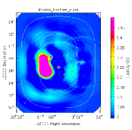
Figure 12: Mosaic Spectral Cube from Feathering (LEFT) and Joint SDINT reconstruction (RIGHT) at 1.0GHz, 1.5GHz and 2.0GHz (top to bottom).

Figure 13: Wideband MT-MFS Mosaic Intensity and Spectral index from INT data only

Figure 14: Wideband MT-MFS Mosaic Intensity and Spectral index from Feathering

Figure 15: Wideband MT-MFS Mosaic Intensity and Spectral index from Joint SDINT reconstruction

A series of joint mosaic imaging tests were done using the simulated mosaic interferometer data along with the single dish images. The A-Projection algorithm offered by the gridder=’mosaic’ option in CASA’s tclean was used with a flat-noise normalization and used the same frequency dependent primary beam models that were used for the simulation of the mosaic interferometer data.

Figures 11 and 12 show flat-sky results for mosaic spectral cube imaging using the INT-only, SD-only, Feathering and Joint SDINT approaches. Artifacts due to missing short spacing information are clearly visible in the INT-only images, less prominent in the feathering results and minimized in the joint SDINT reconstructions where the on-source structure and flux values are closest to the expected true intensity distribution (shown in Fig.3). In all these figures, interferometry primary beam contours are drawn at the 0.5 and 0.9 gain levels and they illustrate the algorithms’ performance both within the central region of the mosaic as well as at the edge (where normalization errors, if present, would most prominently manifest themselves).

Figure 15 shows flat-sky intensity and spectral index maps for the interferometer-only wideband mosaic reconstruction. The spectral index recovery at the largest scales is more accurate than the basic single pointing simulation,but still too steep by about 0.5 or more. Figure 15 shows results from feathering the Taylor coefficient maps from the above interferometer-only reconstruction (after taking them to flat-sky) with single dish wideband Taylor coefficients derived from the SD-only multi-term deconvolution run. Figure 15 shows results from the joint SDINT method which produced the most accurate of the results shown here.

6.3 Effect of relative noise levels

Figure 16: With Noise : Wideband MT-MFS Mosaic Intensity and Spectral index from Noisy INT data alone

Figure 17: With Noise : Wideband MT-MFS Intensity and Spectral index from Noisy SD data alone

Figure 18: With Noise : Wideband MT-MFS Mosaic Intensity and Spectral index from Joint SDINT reconstruction with sdgain=1.0

Figure 19: With Noise : Wideband MT-MFS Mosaic Intensity and Spectral index from Joint SDINT reconstruction with sdgain=0.2

Noise in a single dish image is often higher than in the interferometric image and a typical feathering approach will result in a degradation of noise level. Careful matching of noise levels may require suppressing the flux or using complicated spatial-frequency weighting functions that attempt to balance the competing requirements of flux correctness versus noise suppression. However, as discussed in section 5.2 one can in principle separate the step of flux scaling from that of applying relative weights within a joint reconstruction scheme to suppress noise introduced by the single dish data while still preserving flux correctness in the reconstruction. A basic demonstration of this idea has been explored in this paper with results shown in Figures 19 to 19.

In a test designed specifically to evaluate the use of relative weighting to control single dish noise levels, random Gaussian noise of 0.2 Jy was added per simulated visibility value to produce a 0.002 Jy/beam image rms level for the interferometer data, a peak-to-noise dynamic range of 150 for the extended emission with a peak flux of 0.3 Jy/beam and a dynamic range of about 500 for the 1 Jy point sources. Random Gaussian noise of 0.02 Jy was added per pixel of the simulated single dish image prior to smoothing by the SD beam. The resulting single dish image noise level was 0.3 Jy/beam, had a peak-to-noise dynamic range of about 50 for the extended structures and with the point sources not visible above the noise. This simulates the situation where sky noise dominates and produces an image error pattern at scales larger than the pixel size or gridding kernel. Such noise is harder to suppress or filter out without affecting the source structure itself and was chosen in order to evaluate the harder extreme of the problem.

Only the wideband multi-term mosaic imaging runs were repeated for these tests with noise. Figs.19 and 19 show results with the INT only and SD only data (compare with Figs.9 and 9). While the interferometer reconstruction is relatively unchanged compared to the noiseless simulation, the single dish reconstructions of both intensity and spectral index are strongly affected by noise at the scale of the single dish beam. Fig.19 shows results from the joint SDINT reconstruction when the single dish data were given equal weight compared to the interferometer data (i.e. sdgain = 1.0 in CASA Feather used within the SDINT algorithm). The maps show errors that track the noise pattern of the SD-only images at a level of 0.004 Jy/beam. Fig.19 shows results when the single dish data were downweighted (i.e. sdgain=0.2). The intensity map clearly shows an improvement in the noise level (now at 0.0022 Jy/beam, compared to the INT only noise level of 0.002 Jy/beam) with on-source intensity and spectral index closer to the truth. The improvement on the spectral index in this instance was only minor and further reduction of the single dish gain factor began to reach the edge of the viable range for this simulation and resulted in increased steepness of the reconstructed spectral index.

In practice, a general rule of thumb for choosing a scale factor for noise suppression is to compare the noise levels between an INT only reconstruction and an SDINT reconstruction with sdgain=1.0, keeping in mind that the noise adds in quadrature to produce the observed SDINT level. The derived sdgain factor may then be used only if it is within the viable range driven by uv-coverage and sky structure for the particular observation at hand.

These results suggest that the idea of downweighting the single dish data during combination may yield useful improvements in imaging quality but that it must be done with caution especially if there are significant errors at large spatial scales where the interferometer data too do not provide sufficient constraints (which is precisely what this test probed). In situations where the single dish noise is at smaller spatial scales (such as instrumental noise that is independent per measurement and smeared only by the imaging gridding kernel) this approach is likely to be more effective.

This view has potentially positive implications on the required time on source for a single dish and an interferometer. For example, for the ALMA telescope, Mason (2013) derive relative observation times between the ALMA 12m array, the ACA 7m array and the ALMA 12m Total Power array that are required to match visibility noise levels in preparation for a single step feathered combination. However, for sources with significant flux in extended structures, relaxing this requirement would imply the need for less observing time for the single dish data than is currently the standard.

In conclusion, as long as the single-dish data are downweighted within the viable range (from the uv-coverage and structure point of view), the noise may be suppressed with minimal consequences on the final reconstruction.

7 Discussion

Missing short spacing information in interferometric data results in incorrect reconstructions of the structure and especially the spectrum of the sky brightness distributions at large spatial scales. Single dish observations can effectively provide sufficient constraints to reconstruct these structures and spectra accurately.

Several techniques have been in use for decades, but there is no established standard especially for wideband imaging. In this paper we have evaluated several methods and proposed the SDINT algorithm. We have demonstrated that it can accurately solve the problem of missing short spacings as encountered during a wideband reconstruction and it can do this within a generic joint reconstruction algorithmic framework that supports spectral cubes or wideband multi-term reconstruction, narrow-field or wide-field mosaic imaging as well as the option to include only interferometer data or single dish data or both together. In the context of widely differing noise levels between the single dish and interferometer data, we have also evaluated the idea of using relative weighting between the single dish and interferomter data to achieve low joint image rms levels without sacrificing flux accuracy.

Future work will include real-world applications to VLA and GBT wideband mosaic imaging and ALMA’s 12m, 7m and 12m total power combinations for spectral cube and continuum imaging. The option of including a single dish major cycle that operates directly with ALMA total-power data is within reach within the CASA software and it will be useful to evaluate its numerical benefits. The idea of downweighting single dish data requires careful evaluation on real data for specific telescope and observing setups (to allow evaluation for specific types of uv-coverage), but has the potential of reducing the amount of required single dish observing time. Finally, various weighting schemes discussed in the literature (e.g. in Koda et al. (2011) and Kurono et al. (2009)) will also be evaluated and adopted within the SDINT implementation.

All the above steps are in progress as part of commissioning the algorithm for production use and will result in software documentation and usage guidelines for different applications.

8 Acknowledgements

The initial part of this research was conducted under the NRAO Summer Student Research Assistantship programme and continued within the NRAO Algorithm R&D group. We acknowledge the use of the CASA software and the PySynthesisImager python level prototyping interface to its imaging libraries. We would like to thank S.Bhatnagar and K.Golap of NRAO for participating in discussions on details of this work. The National Radio Astronomy Observatory is a facility of the National Science Foundation operated under cooperative agreement by Associated Universities, Inc.

References

- AIPS_Docs (2017) AIPS_Docs. 2017, Task IMERG
- Bhatnagar et al. (2008) Bhatnagar, S., Cornwell, T. J., Golap, K., & Uson, J. M. 2008, Astron. & Astrophys., 487, 419
- Bhatnagar et al. (2013) Bhatnagar, S., Rau, U., & Golap, K. 2013, ApJ, 770, 91
- CASA_Docs (2017) CASA_Docs. 2017, Feather and CASAFeather
- CASA_Docs (2018) —. 2018, Synthesis Imaging
- Clark (1980) Clark, B. G. 1980, Astron. & Astrophys., 89, 377
- Cornwell (2008) Cornwell, T. J. 2008, IEEE Journal of Selected Topics in Signal Processing, issue 5,, 2, 793
- Cornwell & Evans (1985) Cornwell, T. J., & Evans, K. J. 1985, Astron. & Astrophys., 143, 77
- Cornwell et al. (2008) Cornwell, T. J., Golap, K., & Bhatnagar, S. 2008, IEEE Journal of Selected Topics in Signal Processing, 2, 647
- Cotton (2017) Cotton, W. D. 2017, Publications of the Astronomical Society of the Pacific, 129, 094501
- Högbom (1974) Högbom, J. A. 1974, Astron. & Astrophys. Suppl. Ser., 15, 417
- Junklewitz et al. (2016) Junklewitz, H., Bell, M. R., Selig, M., & Enßlin, T. A. 2016, aap, 586, A76
- Koda et al. (2011) Koda, J., et al. 2011, apjs, 193, 19
- Kurono et al. (2009) Kurono, Y., Morita, K.-I., & Kamazaki, T. 2009, pasj, 61, 873
- Mangum et al. (2007) Mangum, J. G., Emerson, D. T., & Greisen, E. W. 2007, aap, 474, 679
- Mason (2013) Mason, B. S., B. C. 2013, Relative Integration times for the ALMA 12-m, 7-m and Total Power Arrays, Tech. rep., NAASC, NRAO
- MIRIAD_Docs (2013) MIRIAD_Docs. 2013, Task IMMERGE
- Rau et al. (2009) Rau, U., Bhatnagar, S., Voronkov, M. A., & Cornwell, T. J. 2009, Proc. IEEE, 97, No. 8, 1472
- Rau & Cornwell (2011) Rau, U., & Cornwell, T. J. 2011, aap, 532, A71
- Sault et al. (1996) Sault, R. J., Staveley-Smith, L., & Brouw, W. N. 1996, aaps, 120, 375
- Sault & Wieringa (1994) Sault, R. J., & Wieringa, M. H. 1994, Astron. & Astrophys. Suppl. Ser., 108, 585
- Schwab & Cotton (1983) Schwab, F. R., & Cotton, W. D. 1983, AJ, 88, 688