Topological thermal Hall effect of “magnetic monopoles”
in pyrochlore U(1) spin liquid

Abstract

“Magnetic monopole” is an exotic quantum excitation in three dimensional U(1) spin liquid, and its emergence is purely of quantum origin and has no classical analogue. We predict topological thermal Hall effect (TTHE) of “magnetic monopoles” and present this prediction through non-Kramers doublets on a pyrochlore lattice. We observe that, when the external magnetic field polarizes the Ising component of the local moment, internally this corresponds to the induction of emergent dual U(1) gauge flux for the “magnetic monopoles”. The motion of “magnetic monopoles” is then twisted by the induced dual U(1) gauge flux. This emergent Lorentz force on “magnetic monopoles” is the fundamental origin of TTHE. Therefore, TTHE would be a direct evidence of the “monopole”-gauge coupling and the emergent U(1) gauge structure in pyrochlore U(1) spin liquid. Our result does not depend strongly on our choice of non-Kramers doublets for our presentation, and can be well extended to Kramers doublets. Our prediction can be readily tested among the pyrochlore spin liquid candidate materials. We give a detailed discussion about the expectation for different pyrochlore magnets.

I Introduction

Emergent gauge structure and theory comprise an important subject in modern condensed matter physics, particularly for strongly correlated quantum matter Wen (2004). It is this theory that underlies the unified gauge theory description of fractional quantum Hall effect and quantum spin liquids (QSLs) Wen (2004). While an initial understanding of the fractional quantum Hall effect(FQHE) relies on Laughlin’s construction of a variational wave-function Laughlin (1983), later on, Ginzburg-Landau field theoretical descriptions are developed conceiving an additional gauge interaction described by the Chern-Simons gauge theories Zhang et al. (1989); Lopez and Fradkin (1991). The discovery of QSLs follows a completely independent line of development pioneered by Anderson and collaborators Anderson (1973); ANDERSON (1987); Baskaran et al. (1987). Intriguingly, a QSL state, dubbed as ‘chiral spin liquid’ state, is proposed to be equivalent to the FQHE Kalmeyer and Laughlin (1987). And, the modern understanding of QSLs has been greatly advanced by various lattice gauge theories Savary and Balents (2017a); Senthil and Fisher (2000); Hermele et al. (2004) conceiving non-local, fractionalized excitations. To confirm the existence of QSLs in a realistic quantum material, one has to establish the presence of the emergent gauge structure and the associated fractionalized quantum particles, e.g., the spinon and “magnetic monopole” in U(1) QSL. This requires a mutual feedback between theories and experiments. More precisely, one needs to understand how the emergent gauge structure manifests itself in the actual experimental observables. In a more progressive manner, it would be beneficial to provide some level of controllability or prediction of these emergent phenomena from the understanding of the relationship between the microscopic physics and the emergent gauge structure. In this effort, some of us have proposed ways to spectroscopically control the spinon band structure and then the spinon continuum in the inelastic neutron scattering measurement for several QSL candidates Li and Chen (2017a, b); Li et al. (2017); Yao-Dong Li and Gang Chen (2019) such as Ce₂Sn₂O₇, Ce₂Zr₂O₇ and YbMgGaO₄ Sibille et al. (2015); Gao et al. (2019); Li et al. (2015a); Shen et al. (2018, 2016); Li et al. (2016); Zhang et al. (2018); Paddison et al. (2017); Li et al. (2015b). As for the transport properties, two of us have further studied the strong Mott insulating QSLs and suggested the origin of the emergent Lorentz force from the antisymmetric Dzyaloshinskii-Moriya interaction for the spinons as the source of the topological thermal Hall conductivity in these systems Yong Hao Gao and Gang Chen (2019); Gao et al. (2019). In this paper, we turn our attention to study the thermal Hall transport in another important QSL state, namely the pyrochlore U(1) QSL.

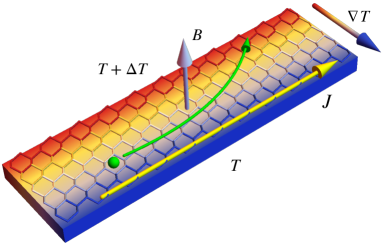
Figure 1: (Color online.) Schematic picture of the thermal Hall effect from the “magnetic monopoles” on the dual diamond lattice for the pyrochlore U(1) QSL, where the heat current “$J$” has contributions from all mobile excitations. We single out the “magnetic monopoles” (in green) that are suggested to contribute to the thermal Hall effect in this work.

The pyrochlore U(1) QSL is described by the emergent compact U(1) lattice gauge theory, and supports the gapless U(1) gauge photon, gapped spinon and “magnetic monopole” as its elementary excitations Hermele et al. (2004). Many pyrochlore materials, mainly the rare-earth pyrochlores Gingras and McClarty (2014); Lee et al. (2012); Molavian et al. (2007); Onoda and Tanaka (2011); Benton et al. (2012); Taillefumier et al. (2017); Savary and Balents (2017a), have been proposed as candidates to realize this U(1) QSL (Savary and Balents, 2017a). Although many interesting experimental signatures have been suggested, the firm establishment of pyrochlore U(1) QSL has not yet been settled for any material. In this paper, we develop a theory to predict the phenomenon of the topological thermal Hall effect (TTHE) in the pyrochlore U(1) QSL and propose it as a positive evidence of the emergent U(1) gauge structure. Our observation stems from the physical meaning of the spin variables in the U(1) QSL. It is observed that, the Ising component of the spin works as an emergent electric field in the U(1) lattice gauge theory. From the view of the dual gauge theory, this emergent and internal electric field behaves as a dual U(1) gauge flux for the “magnetic monopoles.” The external magnetic field, that couples linearly with the spins through a simple Zeeman coupling, polarizes the internal electric field and thereby modifies the dual U(1) gauge flux that is experienced by the “magnetic monopoles.” This coupling between the internal variable and the external field effectively generates an emergent Lorentz force on the “magnetic monopoles” and creates a TTHE in the system. The dual Hamiltonian for the “magnetic monopoles,” that captures this effect, is given as

$${\cal H}_{\rm dual}= -t\sum_{\langle\textsf{r}\textsf{r}^{\prime}\rangle}\Phi^{\dagger}_{\textsf{r}}\Phi_{\textsf{r}^{\prime}}e^{-i2\pi a_{\textsf{r}\textsf{r}^{\prime}}}-\mu\sum_{\textsf{r}}\Phi^{\dagger}_{\textsf{r}}\Phi_{\textsf{r}}$$ (1)

$$+\sum_{rr^{\prime}}\frac{U}{2}({\rm curl}a-\bar{E}_{rr^{\prime}})^{2}-K\sum_{\textsf{r}\textsf{r}^{\prime}}\cos B_{\textsf{r}\textsf{r}^{\prime}},$$

where $\Phi^{\dagger}_{\textsf{r}}$ $(\Phi_{\textsf{r}})$ denotes a creation (annihilation) operator of the “magnetic monopoles” on a dual diamond lattice r-site. Here the sherif symbol r is reserved for the dual diamond lattice that will be explain later. The first line describes the hopping of the “magnetic monopoles” on the dual diamond lattice and minimally couples to the dual dynamical U(1) gauge field $a_{\textsf{r}\textsf{r}^{\prime}}$, and the second line is the Maxwell term of the U(1) gauge field. The detailed description of the notation in Eq. (1) is given in Sec. II. The external magnetic field modifies the dual U(1) gauge flux in the above equation and generates the TTHE for the “magnetic monopoles”, which is explained in Sec. III.

Thermal Hall effect has been measured and detected in the pyrochlore ice materials Tb₂Ti₂O₇ Hirschberger et al. (2015) and Yb₂Ti₂O₇ Max Hirschberger, Peter Czajka, S. M. Koohpayeh, Wudi Wang, and N. Phuan Ong (2019). In Tb₂Ti₂O₇, the crystal electric field ground state of the Tb³⁺ ion under the $D_{3d}$ crystal electric field is a non-Kramers doublet Molavian et al. (2007), although the crystal field gap to the first excited doublet is relatively small among the rare-earth pyrochlore magnets. In Yb₂Ti₂O₇, the crystal electric field ground state of the Yb³⁺ ion is a Kramers doublet. In this paper, we will first deliver our theory with the non-Kramers doublets for the pyrochlore ice U(1) QSL and then explain the extension to the Kramers doublets. Although we start with the spin ice manifold, our results do not rely on the proximity of the spin ice configuration. As long as the pyrochlore U(1) QSL is realized, our results would be applicable, regardless whether the system is close or not close to the spin ice manifold.

The remaining parts of the paper are organized as follows. In Sec. II, we construct the dual lattice gauge theory for the pyrochlore U(1) QSL and introduce the “magnetic monopole” degrees of freedom into the formulation. In Sec. III, we present the induction of dual U(1) gauge flux through the Zeeman coupling. The thermal Hall current for the “magnetic monopoles” under a temperature gradient is analyzed in Sec. IV.1 . In Sec. IV.2, we calculate the “monnopole” band dispersion from the mean-field monopole Hamiltonian with an induced dual U(1) gauge flux. In Sec. IV.3 the temperature dependence of the thermal Hall conductivity is calculated. We compare our results with other QSLs in Sec. V and give a detailed discussion about the expectation for different pyrochlore magnets. The details of calculation and derivation are presented in Appendices.

Excitations (notation 1)	Excitations (notation 2)
Spinon	Magnetic monopole
“Magnetic monopole”	Electric monopole
Gauge photon	Gauge photon

Table 1: Correspondence between two different notations for the elementary excitations in pyrochlore U(1) QSL. “Magnetic monopole” is sometimes referred as visons in some literature. Usually “vison” refers to the $\mathbb{Z}_{2}$ flux Senthil and Fisher (2000, 2001a, 2001b) for the $\mathbb{Z}_{2}$ topological order in 2+1D and is also known as “m” particle in Kitaev’s toric code model Kitaev (2003).

II “Magnetic monopoles’ from dual lattice gauge theory

There are two realistic spin models proposed for the pyrochlore U(1) QSL Huang et al. (2014); Ross et al. (2011); Onoda and Tanaka (2011). Due to the spin-orbit entangled nature of the relevant rare-earth ion, the spin models are highly anisotropic. One of the spin models applies for usual Kramers doublets as well as non-Kramers doublets. For instance, the ground state of the Yb³⁺ ion in Yb₂Ti₂O₇ and Er³⁺ ion in Er₂Ti₂O₇ Ross et al. (2011); Savary et al. (2012) are Kramers doublets, while the ground state of the Pr³⁺ ion in Pr₂Zr₂O₇ Wen et al. (2017) and Tb³⁺ ion in Tb₂Ti₂O₇ Onoda and Tanaka (2011) are non-Kramers doublets. The other model, known as the XYZ model Huang et al. (2014); Li and Chen (2017a), applies for dipole-octuple doublets, such as Nd³⁺ ion in Nd₂Zr₂O₇ Petit et al. (2016) and Ce³⁺ ion in Ce₂Sn₂O₇ and Ce₂Zr₂O₇ Sibille et al. (2015); Gao et al. (2019). It is known that both spin models reduce to a XXZ model in certain limit, and the XXZ model on a pyrochlore lattice supports a pyrochlore quantum ice U(1) QSL Hermele et al. (2004). Generically, this QSL state is a stable phase derived from the generic spin models. Although theoretical approaches are valid in the Ising regime Hermele et al. (2004), the stability of the pyrochlore U(1) QSL goes beyond the perturbative Ising regime Lee et al. (2012). Therefore, we adopt a more inclusive notion of “pyrochlore U(1) QSL”. In this section, we first start from the ring exchange model that is obtained from the realistic spin model by the degenerate perturbation theory in the Ising limit. The discussion is on a generic ground where the local moment is not specified to be a Kramers doublet or non-Kramers doublet. Then, we obtain a lattice gauge theory and expose the “monopoles” explicitly by means of electromagnetic duality transformation.

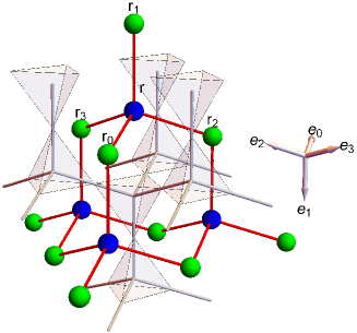
Figure 2: (Color online.) Diamond lattice (in gray line) and the dual diamond lattice (in red line). The physical spin is located in the middle of the link on the diamond lattice. The diamond lattice is formed by the tetrahedral centers of the original pyrochlore lattice. The spinons (“magnetic monopoles”) hop on the diamond (dual diamond) lattice. The colored balls correspond to the position of “magnetic monopoles.”

The pyrochlore U(1) QSL for the effective spin-1/2 moments can be accessed by a ring exchange model Hermele et al. (2004)

$${\cal H}_{\rm ring}= -\frac{K}{2}\sum_{\hexagon_{p}}(\tau_{1}^{+}\tau_{2}^{-}\tau_{3}^{+}\tau_{4}^{-}\tau_{5}^{+}\tau_{6}^{-}+{\rm H.c.})$$ (2)

where $K$ is a renormalized energy scale for the low-energy effective theory. Here the spin operators are ${\tau^{\pm}_{i}=\tau^{x}_{i}\pm i\tau^{y}_{i}}$. A $z$-direction is defined locally along the $\langle 111\rangle$-direction of each site. An elementary hexagonal ring “$\hexagon_{p}$” is formed by six neighboring sites ${i=1,...,6}$ on the pyrochlore lattice, and the subindex “$p$” refers to the pyrochlore lattice. One can transform the ring exchange model into a compact U(1) lattice gauge theory (LGT) Hermele et al. (2004); Savary and Balents (2012),

$${\cal H}_{\rm LGT}= -K\sum_{{\hexagon_{d}}}\cos\big{[}{\rm curl}A\big{]}+\frac{U}{2}\sum_{rr^{\prime}}\big{(}E_{rr^{\prime}}-\frac{\epsilon_{r}}{2}\big{)}^{2}$$ (3)

by introducing a pair of lattice gauge fields, i.e., electric field ${E_{rr^{\prime}}=\tau_{i}^{z}+1/2}$ and vector gauge potential ${e^{\pm iA_{rr^{\prime}}}=\tau_{i}^{\pm}}$. These fields are defined on the nearest-neighbor diamond links $rr^{\prime}$, where $r$ and $r^{\prime}$ are used to label the diamond lattice sites. The pyrochlore site $i$ sits at the mid-point of the corresponding link $rr^{\prime}$. Two distinct sublattices $r({\rm\in\text{I}}),r^{\prime}({\rm\in II})$ reside at the centers of two corner sharing tetrahedra of the pyrochlore lattice. $E_{rr^{\prime}}$ (integer-valued) and $A_{rr^{\prime}}$ ($2\pi$-periodic) form a pair of conjugated fields satisfying ${[E_{rr^{\prime}},A_{r_{1}r_{1}^{\prime}}]=i\delta_{rr_{1},r^{\prime}r_{1}^{\prime}}}$. The lattice curl is defined as summation over all bonds of a diamond hexagon ${{\rm curl}\,A=\sum_{rr^{\prime}\in{\hexagon_{d}}}A_{rr^{\prime}}}$. Here “$\hexagon_{d}$” refers to the elementary hexagon on the diamond lattice formed by the tetrahedral centers of the pyrochlore lattice. Additionally, an electric field stiffness $U$ term is added, where ${\epsilon_{r}=+1\,(-1)},{r\in{\rm I}\,({\rm II})}$. In the large $U$ limit, the Hilbert space of the LGT is properly casted back to the microscopic spin-1/2 local moment. In the low energy and long distance limit, the actual $U$ is renormalized compared to the original lattice level.

“Magnetic monopole” is the topological defect of emergent U(1) gauge potential, and is the source and sink of the internal magnetic fields. Unlike the spinons that reside on the tetrahedral centers of the pyrochlore lattice (or the diamond lattice sites), the “magnetic monopoles” live on the dual diamond lattice. In the above electric field and gauge field representation, the “magnetic monopole” variable is not explicit. An electromagnetic duality transformation is performed on the LGT to expose this variable Hermele et al. (2004); Chen (2017a). Although this is covered in the literature extensively, some steps of the derivation are not mathematically straightforward. We carry out the duality transformation in Appendices A and B, where a special care has been taken for the diamond lattice structure. The expression of the dual Hamiltonian is presented here,

$${\cal H}_{\rm dual}[\theta,a,B] = \sum_{\langle rr^{\prime}\rangle}\frac{U}{2}({\rm curl}a_{rr^{\prime}}-\bar{E}_{rr^{\prime}})^{2}-\sum_{\langle\textsf{r}\textsf{r}^{\prime}\rangle}K\cos B_{\textsf{r}\textsf{r}^{\prime}}$$ (4)

$$-t\sum_{\textsf{r}\textsf{r}^{\prime}}\cos(\theta_{\textsf{r}}-\theta_{\textsf{r}^{\prime}}+2\pi a_{\textsf{r}\textsf{r}^{\prime}})$$

where $\textsf{r},\textsf{r}^{\prime}$ represent dual diamond lattice sites as plotted in Fig. 2. A rotor variable $e^{\pm i\theta_{\textsf{r}}}$ is proven to be the creation/annihilation operator of the “magnetic monopole” (see Appendix B). We restore the bosonic nature of the “magnetic monopole” variable by introducing $\Phi_{\textsf{r}}\equiv\rho_{\textsf{r}}e^{i\theta_{\textsf{r}}}$, where a unimodular condition $|\Phi_{\textsf{r}}|=1$ is often imposed if one abandons the heavier amplitude fluctuations. We arrive at the dual Hamiltonian presented in Eq. (1). The dual theory describes the “magnetic monopole” $\Phi_{\textsf{r}}$ hopping on the dual diamond lattice and minimally coupled to a dual U(1) gauge field. The dual U(1) gauge field $a_{\textsf{r}\textsf{r}^{\prime}}$ (real-valued) and magnetic field $B_{\textsf{r}\textsf{r}^{\prime}}$ ($2\pi$-periodic) are defined on the link $\textsf{r}\textsf{r}^{\prime}$ of the dual diamond lattice. These dual fields are related to the field in the original representation by,

$${\rm curl}\,a\equiv\sum_{\textsf{r}\textsf{r}^{\prime}\in\hexagon_{d}^{\ast}}a_{\textsf{r}\textsf{r}^{\prime}}=E_{rr^{\prime}}-E^{0}_{rr^{\prime}},$$ (5)

$$B_{\textsf{r}\textsf{r}^{\prime}}={\rm curl}\,A\equiv\sum_{rr^{\prime}\in{\hexagon_{d}}}A_{rr^{\prime}},$$

where the dual hexagonal ring is labelled by $\hexagon_{d}^{\ast}$. The dual lattice curl is defined as summation over all bonds of a dual hexagon. The definitions in Eq. (5) guarantee that the commutation relation is satisfied ${[B_{\textsf{r}\textsf{r}^{\prime}},a_{\textsf{r}_{1}\textsf{r}^{\prime}_{1}}]=i\delta_{\textsf{r}\textsf{r}_{1},\textsf{r}^{\prime}\textsf{r}^{\prime}_{1}}}$. A background electric field $E^{0}_{rr^{\prime}}$ is introduced in Eq. (5) to ensure the lattice curl of dual gauge field is divergenceless. Without loss of generality, we choose a specific 2-in-2-out spin-ice configuration for the background electric field, e.g.,

$$E^{0}_{r,r+\epsilon_{r}e_{0}}= E^{0}_{r,r+\epsilon_{r}e_{1}}=\epsilon_{r},$$ (6)

$$E^{0}_{r,r+\epsilon_{r}e_{2}}= E^{0}_{r,r+\epsilon_{r}e_{3}}=0.$$

For the future reference, we define another electric field composed of the background electric field and an offset field,

$$\bar{E}_{rr^{\prime}}= E^{0}_{rr^{\prime}}-\frac{\epsilon_{r}}{2}.$$ (7)

III Induction of dual U(1) gauge flux by Zeeman coupling

The pyrochlore U(1) QSL is in the deconfined phase of the 3+1D LGT. It supports both deconfined spinons and deconfined “magnetic monopoles,” as well as the gapless U(1) gauge photon Hermele et al. (2004) (see Table 1). In the inelastic neutron scattering experiments, these executions correspond to the continuous excitations in the spectrum. The content of the continuum is actually related to the nature of the local moments, which is elucidated in Refs. Chen, 2017a; Yao-Dong Li and Gang Chen, 2019. The $\tau^{z}$-$\tau^{z}$ correlation contains the information of both the (gapped) “magnetic monopole” continuum and the (gapless) gauge photon Chen (2017a). Moreover, the spectral structure of the continuum is intimately tied to the symmetry fractionalization of the spinons and “magnetic monopoles” Chen (2017a); Yao-Dong Li and Gang Chen (2019); Chen (2017b). Although these results are quite useful, they are all consequences of the deconfinement and fractionalization, not a direct evidence of the matter-gauge coupling. To demonstrate the consequence of the matter-gauge coupling, let us consider the Landau level physics in the system of electrons. The Coulomb interaction between the electrons is the consequence of the facts that the electron carries the U(1) gauge charge and the photon mediates the interaction through the electron-photon coupling. The electron-gauge coupling of the electrons can be revealed through the quantum oscillation of a metal in external magnetic fields, which arises from the population of electronic Landau levels . In our case, the “magnetic monopole” is coupled to the internal dual U(1) gauge field, and the “magnetic monopole” is bosonic and gapped. So there does not exist the usual quantum oscillation. Moreover, the internal U(1) gauge flux is not obviously tunable. Our key observation is that the external field could generate an internal dual U(1) gauge flux for the “magnetic monopoles.” This is already pointed in Sec. I. In the following, we embark on explaining this point with the non-Kramers doublets.

For the non-Kramers doublets, only the local $z$-component of the effective spin is odd under the time reversal symmetry. The Zeeman coupling of the effective spin to the external field is given as

$${\cal H}_{\rm Zeeman}= -H_{0}\sum_{i}({\hat{n}}\cdot{\hat{z}}_{i})\tau_{i}^{z}$$ (8)

$$\simeq -H_{0}\sum_{\langle rr^{\prime}\rangle}({\hat{n}}\cdot{\hat{z}}_{i})({\rm curl}\ a_{rr^{\prime}}-\bar{E}_{rr^{\prime}}),$$

where the first line is written with the microscopic spin language while the second line is expressed in terms of the emergent variables in the pyrochlore U(1) QSL phase. Here the link $\langle rr^{\prime}\rangle$ on the diamond lattice is identical to the pyrochlore lattice site $i$, $\hat{n}$ defines the direction of the magnetic field, and ${\hat{z}}_{i}$ denotes the local $z$-direction of on the lattice site $i$. A weak external magnetic field polarizes the spins in each pyrochlore tetrahedron partially, and throughout we work in the weak field regime such that the U(1) QSL state is preserved, namely the lattice gauge theory is in its deconfined phase. Hence, the “magnetic monopole” representation in Eq. (1) remains to be a valid picture for the system.

The Zeeman coupling term enters into the dual Hamiltonian Eq. (1) as a modification of the background electric field distribution,

$${\cal H}_{\rm dual}(H_{0})= \sum_{\langle rr^{\prime}\rangle}\frac{U}{2}({\rm curl}\ a_{rr^{\prime}}-\bar{E}^{\prime}_{rr^{\prime}})^{2}-\cdots$$ (9)

$$\bar{E}^{\prime}_{rr^{\prime}}=\bar{E}_{rr^{\prime}}+\frac{H_{0}}{U}({\hat{n}}\cdot{\hat{z}}_{i}).$$

We observe that the external field modifies the internal dual U(1) gauge flux and thereby generates an emergent Lorentz force on the “magnetic monopoles.” The motion of the “magnetic monopoles” will be twisted by the induced dual U(1) gauge flux, giving rise to the TTHE of “magnetic monopoles.” This is a direct manifestation and unbiased signature of the emergent “monopole”-gauge coupling. This phenomenon serves as an analog of the Lorentz force for the electron motion on the lattice, except that the Lorentz force here is emergent and arises from the induction of the internal dual U(1) gauge flux via the Zeeman coupling.

The Zeeman coupling depends sensitively on the local crystal field axis. Thus, the induced dual U(1) gauge flux depends on the lattice geometry and the field orientation, i.e., the mean field value of dual gauge flux $\langle{\rm curl}\ a\rangle$ is related to the induced local magnetization $\langle\tau^{z}\rangle$. Without the Zeeman field, the dual U(1) gauge flux is $\pi$ for the elementary hexagon on the dual diamond lattice. The Zeeman coupling breaks the time reversal symmetry and shifts the dual U(1) gauge flux from $\pi$ by a finite portion

$$2\pi\langle{\rm curl}\ a_{rr^{\prime}}\rangle= \pi+2\pi\frac{H_{0}}{U}({\hat{n}}\cdot{\hat{z}}_{i})\quad{\rm mod}\,(2\pi),$$ (10)

where $\langle{\rm curl}\ a_{rr^{\prime}}\rangle$ represents a mean-field solution for the dual gauge flux. The parameter $U$ is often unknown. Physically, the induced flux can be obtained from the induced local magnetization that is given as,

$$\langle\tau^{z}_{i}\rangle\equiv\chi_{i}(\hat{n}\cdot\hat{z}_{i})H_{0},$$ (11)

which depends on the local spin susceptibility $\chi_{i}$ along the $z$-direction on each site $i$. In the weak field limit, $\chi_{i}$ should be uniform by definition and symmetry requirement. It is also a constant due to the strong spin-orbit coupling in the system. The above equations give us the relations between the induced dual U(1) flux and the physical magnetization.

With the mean-field solution of dual U(1) gauge flux in the presence of the Zeeman field, we write down a mean-field Hamiltonian for the “magnetic monopoles,”

$${\cal H}_{\rm MF}=-\frac{t}{2}\sum_{\textsf{r}\textsf{r}^{\prime}}e^{-i2\pi a^{0}_{\textsf{r}\textsf{r}^{\prime}}}\Phi^{\dagger}_{\textsf{r}^{\prime}}\Phi_{\textsf{r}}+{\rm H.c.}-\mu\sum_{\textsf{r}}\Phi^{\dagger}_{\textsf{r}}\Phi_{\textsf{r}},$$ (12)

where $a^{0}_{\textsf{r}\textsf{r}^{\prime}}$ represents a gauge choice for the dual U(1) gauge field. The dual gauge field is fixed at a particular mean-field solution, and its conjugate field, namely the internal magnetic field, is omitted. Therefore, the Hamiltonian in Eq. (12) describes the hopping of “magnetic monopoles” in the presence of a dual U(1) gauge field, whose fluctuation has been ignored.

IV Topological thermal Hall effect

In the previous sections, we have explained our ideas and the physical origin of the TTHE for the “magnetic monopoles.” Here we further establish the theoretical framework to demonstrate the TTHE and make specific predictions for the experiments.

IV.1 General framework

To extract information out of the twisted motion of the “magnetic monopoles,” we perturb the system with a temperature gradient in the plane perpendicular to the external magnetic field. In the standard linear response theory, the small external perturbation appears in the Hamiltonian. The effect of the temperature gradient $T({\bf r})\simeq T_{0}[1-\psi({\bf r})]$ takes place in the Boltzmann factor, i.e., $e^{-{\cal H}/k_{\rm B}T({\bf r})}\simeq e^{-[1+\psi({\bf r})]{\cal H}/k_{\rm B}T_{0}}$. Theoretical framework tackling with this problem has been proposed by Luttinger Luttinger (1964). By coupling the Hamiltonian with a pseudo-gravitational potential $\psi({\bf r})$, they are able to incorporate the temperature gradient into a perturbed Hamiltonian $\bar{\cal H}({\bf r})=[1+\psi({\bf r})]{\cal H}$.

We start from the mean-field Hamiltonian in Eq. (12), and treat the dual diamond lattice structure carefully. The pseudo-gravitational potential $\psi_{\textsf{r}}$ couples with an energy density operator ${\cal H}_{\textsf{r}}$. The coupling is turned on for one type of the dual sites with

$$\bar{\cal H}= \sum_{\textsf{r}\in{\rm I}}(1+\psi_{\textsf{r}}){\cal H}_{\textsf{r}},$$ (13)

The energy density operator at a dual site r is defined as

$${\cal H}_{\textsf{r}}=-\frac{t}{2}\sum_{\textsf{r}^{\prime}\in\textsf{r}}e^{-i2\pi a^{0}_{\textsf{r}\textsf{r}^{\prime}}}\Phi_{\textsf{r}^{\prime}}^{\dagger}\Phi_{\textsf{r}}+{\rm H.c.},$$ (14)

where the summation is over four nearest neighbor dual sites $\textsf{r}^{\prime}\in\textsf{r}$, which are labelled in Fig. 2. The chemical potential term is omitted in the energy density operator, since it has no contribution to the transport properties below. The energy density is not modified upon the addition of pseudo-gravitational potential, since the four nearest neighbors necessarily belong to the type-II sites. We work through the lattice version of continuity equation for the energy density operator,

$$\dot{\cal H}_{\textsf{r}}+\sum_{\textsf{r}^{\prime}\in\textsf{r}}{\cal J}^{E}_{\textsf{r}\textsf{r}^{\prime}}=0.$$ (15)

Working through the above continuity equation with the modified local Hamiltonian $(1+\psi_{\textsf{r}}){\cal H}_{\textsf{r}}$, we obtain the modified energy current operator Lee et al. (2015); Matsumoto et al. (2014),

$${\cal J}^{E}_{\textsf{r}\textsf{r}^{\prime}}=(1+\psi_{\textsf{r}^{\prime}}){\cal J}^{0,E}_{\textsf{r}\textsf{r}^{\prime}},$$ (16)

where ${\cal J}^{0,E}_{\textsf{r}\textsf{r}^{\prime}}$ represents the original energy current, which has a form

$${\cal J}^{0,E}_{\textsf{r}\textsf{r}^{\prime}}= \frac{t^{2}}{2}\sum_{\textsf{r}_{1}\in\textsf{r}^{\prime}}i\Phi_{\textsf{r}}^{\dagger}\Phi_{\textsf{r}_{1}}e^{i2\pi(a^{0}_{\textsf{r}\textsf{r}^{\prime}}+a^{0}_{\textsf{r}^{\prime}\textsf{r}_{1}})}+{\rm H.c.}.$$ (17)

Under the choice of a uniform potential gradient Lee et al. (2015), we have ${\psi_{\textsf{r}}={\bf r}_{\bf i}\cdot\nabla\psi}$, where ${\bf r}_{\bf i}$ represents the position of a unit cell ${\bf i}$. The dual lattice links constituting the unit cell ${\bf i}$ are labeled as ${\textsf{r}\textsf{r}^{\prime}\in{\bf i}}$. The choice of this unit cell depends on the dual gauge fixing condition, which is specified in Sec. IV.2. In terms of the unit cell coordinate ${\bf r}_{\bf i}$, we rewrite the modified energy current operator as Lee et al. (2015)

$$J_{\alpha}^{E}({\bf i})= J_{\alpha}^{0,E}({\bf i})+J_{\alpha}^{1,E}({\bf i}),$$ (18)

$$J_{\alpha}^{1,E}({\bf i})= \big{[}J_{\alpha}^{0,E}({\bf i})r^{\beta}_{\bf i}\big{]}\nabla_{\beta}\psi,$$

where $\alpha,\beta=x,y,z$. The energy density vector at the unit cell ${\bf i}$ is defined as,

$$J_{\alpha}^{0,E}({\bf i})=\sum_{\textsf{r},\textsf{r}+\epsilon_{\textsf{r}}e_{\mu}\in{\bf i}}(\epsilon_{\textsf{r}}e_{\mu}\cdot\hat{\alpha}){\cal J}^{0,E}_{\textsf{r},\textsf{r}+\epsilon_{\textsf{r}}e_{\mu}}.$$ (19)

The linear response of the pseudo-gravitational field enters into the energy current expectation value in a two-fold way. Besides the contribution from the distribution function Katsura et al. (2010), there is an additional contribution from the current operator. At the linear order in $\nabla\psi$, we have

$$\langle J_{\alpha}^{E}\rangle={\rm Tr}[\rho_{0}J_{\alpha}^{1,E}]+{\rm Tr}[\rho_{1}J_{\alpha}^{0,E}],$$ (20)

where $\rho_{0}$ is the equilibrium distribution function and $\rho_{1}$ is a first order perturbed distribution function. A statistical force from the temperature gradient is equivalent to a dynamical force induced by pseudo-gravitational potential. The dynamical force acts on the “magnetic monopole” affecting its motion. By counting all the contributions due to the temperature gradient at the first order, the thermal Hall coefficient is calculated and has an expression Matsumoto and Murakami (2011); Matsumoto et al. (2014)

$$\kappa_{xy}= -\frac{k_{\rm B}^{2}T}{N^{3}}\sum_{{\bf k}}\sum_{n=1}^{6}\Big{\{}c_{2}\big{[}g(E_{n,{\bf k}})\big{]}-\frac{\pi^{2}}{3}\Big{\}}\Omega_{n,{\bf k}},$$ (21)

where $c_{2}(x)=(1+x)[\ln(1+x)/x]^{2}-(\ln x)^{2}-{\rm Li}_{2}(-x)$, and ${\rm Li}_{2}(x)$ is a polylogarithmic with ${n=2}$, or the dilogarithm function. Here ${g(\epsilon)=[e^{\epsilon/k_{\rm B}T}-1]^{-1}}$ is the Bose distribution function. $E_{n,{\bf k}}$ is the eigen-energy of the “monopole” Hamiltonian for the $n$’th band at the momentum space ${\bf k}$-point. Here, the Berry curvature and Chern number for the $n$’th band are defined as,

$$\Omega_{n,{\bf k}}=i\langle\partial_{k_{x}}u_{n,{\bf k}}|\partial_{k_{y}}u_{n,{\bf k}}\rangle+{\rm c.c.},$$ (22)

$${\cal C}_{n}(k_{z})=\frac{1}{2\pi}\int_{\rm BZ}dk_{x}dk_{y}\ \Omega_{n,{\bf k}},$$

where $|u_{n,{\bf k}}\rangle$ is the periodic part of the Bloch wave function for the $n$’th band at ${{\bf k}=(k_{x},k_{y},k_{z})}$. The formula indeed shows that the thermal Hall current is generated by the Berry curvature of the “monopole” bands. Due to the time reversal symmetry breaking in the presence of the gauge flux, we can have non-vanishing distribution of Berry curvatures, that gives rise to a finite thermal Hall coefficient.

For our purpose, it is sufficient to consider the TTHE in the presence of the mean-field dual U(1) gauge flux. At the mean-field level, the dual U(1) gauge field is fixed by the background electric field, and the internal magnetic field is absent. The energy current in Eq. (17) is obtained by using the Hamiltonian in Eq. (12). Beyond the mean-field solution, we find that the gauge fluctuations give the thermal current operator a correction. The expression and derivation of this additional contribution is presented in Appendix C. The (gapless) gauge photon contributes directly to the thermal conductivity $\kappa_{xx}$ around the same energy scale as the “magnetic monopoles” except that it remains active down to the lowest energy/temperature and the contribution can directly come from the (fluctuating) Maxwell term. In addition, the spinons would contribute to the thermal effect $\kappa_{xx}$ when the temperature is relatively high to activate spinons. In our current theoretical understanding, the “magnetic monopoles” are singled out to be responsible for the thermal Hall conductivity, and the TTHE in this work refers particularly to the “magnetic monopole” thermal Hall effect.

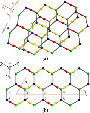
Figure 3: (Color online.) (a) Gauge fixing on the dual diamond lattice. The yellow (red) arrow on the dual links represents a finite phase $\phi=\pi\ (\pi/2)$ picked up by “magnetic monopole” when hopping along the pointed direction. While, the “monopole” hopping on the gray bond is free of the phase, i.e. ${\phi=0}$. (b) A projected view of lattice in the plane perpendicular to $e_{2}$-direction. The dual sites with indexes $1,2,...,8$ constitute a magnetic unit cell. The basis vectors within the plane are labelled by $a_{1},a_{2}$.

IV.2 The modified “magnetic monopole” bands under the magnetic field

To demonstrate the TTHE for the “magnetic monopoles” in the pyrochlore U(1) QSL, we first evaluate the “magnetic monopole” band structure under the magnetic field. Generically speaking, when a generic magnetic field is applied, the “magnetic monopole” should develop a Hofstadter band structure as the induced flux is incommensurate. The corresponding continuum of “magnetic monopoles” in the $\tau^{z}$-$\tau^{z}$ correlation is converted into the continuum from the monopole Hofstadter band. It would be interesting to search for this evolution in the inelastic neutron scattering measurements.

We choose the external field to be aligned in the direction ${{\hat{n}}=\langle 0\bar{1}\bar{1}\rangle}$. To proceed with the mean-field Hamiltonian in Eq. (12), we fix the Zeeman coupling strength such that the dual U(1) gauge flux is commensurate with the lattice. A convenient case is considered here with $H_{0}/U=\sqrt{6}/8$, so that we have

$$2\pi\ {\rm curl}\,a^{0}_{r,r+e_{\mu}}=\left\{\begin{array}[]{cc}\pi-\pi/2,&\ \ \ \ \ \mu=0,\\ \pi+\pi/2,&\ \ \ \ \ \mu=1,\\ \pi+0,&\ \ \ \ \ \mu=2,\\ \pi+0,&\ \ \ \ \ \mu=3.\\ \end{array}\right.$$ (23)

where $a^{0}_{\textsf{r}\textsf{r}^{\prime}}$ represents a gauge choice for the dual U(1) gauge field. The gauge fixing condition on the three-dimensional(3D) dual diamond lattice is illustrated in Fig. 3(a). The yellow (red) arrow on the dual links indicates that a “magnetic monopole” picks up a finite phase $\phi=\pi\ (\pi/2)$ while hopping along the pointed direction. Gray links have zero phases $\phi=0$. The gauge fixing condition is expressed as,

$$2\pi a^{0}_{\textsf{r},\textsf{r}+e_{\mu}}= \xi_{\mu}({\bf q}_{1}\cdot\textsf{r})+\eta_{\mu}({\bf q}_{2}\cdot\textsf{r}),\ \ \ \textsf{r}\in{\rm I},$$ (24)

$${\bf q}_{1}= 2\pi(100),\ \xi_{\mu}=(1001),$$

$${\bf q}_{2}= \pi(100),\ \eta_{\mu}=(0001).$$

where the “monopole” charge is assumed to be unit $q_{m}=1$. With this gauge choice, gauge fields are non-vanishing at the links locating within a quasi-2D plane perpendicular to the $e_{2}$-direction. The dual lattice hexagons form a honeycomb-like structure in this quasi-2D plane. A projected view of the lattice in this plane is illustrated in Fig. 3(b). We define a magnetic unit cell consisting of eight distinct dual diamond sites. A 3D super-lattice is defined by a new set of primitive vectors $a_{\nu},\nu=1,2,3$ with

$$a_{1}=4(e_{0}-e_{3}),$$ (25)

$$a_{2}=e_{0}-e_{1},$$

$$a_{3}=e_{3}-e_{2}.$$

where the basis convention of these vectors and the corresponding reciprocal basis vectors are given in Appendix D.

This is a commensurate case so that one can work out from Eq. (23). The “magnetic monopole” mean-field Hamiltonian is given by,

$${\cal H}_{\rm MF}({\bf k})={\cal H}_{\rm hop}({\bf k})-\mu\,{\bf I}_{8\times 8}$$ (26)

The hopping Hamiltonian takes a particle-hole symmetric form with respect to exchanging type-${\rm I}$ and ${\rm II}$ sublattice sites of the dual diamond lattice,

$${\cal H}_{\rm hop}({\bf k})=-t\left(\begin{array}[]{cc}0&h({\bf k})\\ h^{\dagger}({\bf k})&0\\ \end{array}\right)$$ (27)

with the hopping Hamiltonian between type-${\rm I}$ and ${\rm II}$ sublattice sites given by

$$h({\bf k})=\left(\begin{array}[]{ccccc}e^{ik_{0}}+e^{ik_{1}}&0&0&e^{ik_{3}}+e^{ik_{2}}\\ e^{ik_{3}}e^{i(\pi+\pi/2)}+e^{ik_{2}}&e^{ik_{0}}e^{i\pi}+e^{ik_{1}}&0&0\\ 0&e^{ik_{3}}e^{i\pi}+e^{ik_{2}}&e^{ik_{0}}+e^{ik_{1}}&0\\ 0&0&e^{ik_{3}}e^{i(3\pi/2+\pi)}+e^{ik_{2}}&e^{ik_{0}}e^{i\pi}+e^{ik_{1}}\\ \end{array}\right)$$ (32)

where ${{k_{\nu}\equiv{\bf k}\cdot a_{\nu}},\nu=1,2,3.}$ Due to the particle-hole symmetry, the energy spectrum of ${\cal H}_{\rm hop}({\bf k})$ comes with positive-negative pairs. The four hole bands are plotted in a ($k_{x},k_{y}$) Brillouin zone with a perpendicular momenta ${k_{z}=-3\pi/8}$ (see Fig. 4). A chemical potential to remedy the negative energy situation is added in the mean-field Hamiltonian so that the “magnetic monopole” remains gapped.

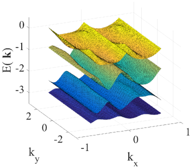
Figure 4: (Color online.) Energy dispersions of $H_{\rm hop}({\bf k})$ for the four hole bands are plotted in the $(k_{x},k_{y})$ Brillouin zone with a perpendicular momentum ${k_{z}=-3\pi/8}$. The unit of momentum $(k_{x},k_{y})$ is $a^{-1}$, with “$a$” being the length of the dual diamond link.

IV.3 Topological thermal Hall effect of “magnetic monopoles”

With the above setup and preparation, we here carry out the calculation for the TTHE of “magnetic monopoles”and show its temperature dependence. First, we evaluate the Berry curvatures for the “monopole” bands. The Berry curvatures of the lowest two “magnetic monopole” bands are plotted in the ($k_{x}$-$k_{y}$) plane with $k_{z}$ locating at the BZ boundary in Fig. 5. The Chern number of the lowest band at any given $k_{z}$ is a positively quantized number ${{\cal C}_{1}(k_{z})=1}$. The second lowest band is endowed with a non-negative, quantized Chern number, namely ${\cal C}_{2}(k_{z})=-1,0$. The two lowest lying bands are of opposite Chern numbers for a majority of $k_{z}$ points.

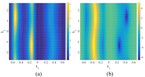
Figure 5: (Color online.) Berry curvatures of the lowest two bands in the ${(k_{x},k_{y})}$ Brillouin zone with the perpendicular momentum ${k_{z}=-3\pi/8}$. The unit of momentum ${(k_{x},k_{y})}$ is $a^{-1}$. (a) The lowest band ${n=1}$; (b) Second lowest band ${n=2}$.

We calculate the thermal Hall coefficient using “monopole” bands in Eq. (26). The temperature dependence of the thermal Hall coefficient $\kappa_{xy}/T$ is depicted in Fig. 6. With the increasing temperatures, $\kappa_{xy}(T)/T$ grows from zero, then, shows a non-monotonic behavior. Eventually, $\kappa_{xy}(T)/T$ drops to zero in the high temperature limit. The trend of this curve can be understood from Eq. (21), which consists of a product of the Berry curvature and a function $c_{2}$. The function $c_{2}(g)$ is a monotonically increasing function of the occupation $g(\epsilon)$, which has a minimum value ${c_{2}=0}$ at ${g=0}$ and saturates to a maximum value $\pi^{2}/3$ in the limit $g\rightarrow+\infty$. In the zero temperature limit, all bands are unoccupied, so that the thermal Hall coefficient vanishes. As the temperature increases, the lowest band starts to have a finite occupancy, giving rise to the increase of $\kappa_{xy}(T)/T$. If we further increase the temperature, the second lowest band, with opposite sign of Berry curvature, are activated, which explains the drop of the curve. Eventually, all bands are equally populated in the high temperature limit, although at very high temperatures the “magnetic monopole” and U(1) QSL simply breaks down. The $\kappa_{xy}(T)/T$ is proportional to the total Chern number, which has a vanishing value. Alternatively, one can vary the chemical potential while keeping the temperature fixed as shown in the inset of Fig. 6. The thermal Hall coefficient decreases along with the chemical potential. The chemical potential shifts all bands into a higher energy regime. The occupation of all bands becomes smaller, which is responsible for the decrease in $\kappa_{xy}(T)/T$.

Finally, we comment on the temperature dependence of the TTHE that takes place along different directions and under different external field strengths. The thermal Hall coefficient $\kappa_{xz}(T)$ shows exact same temperature dependence as $\kappa_{xy}(T)$ with an opposite sign, while $\kappa_{yz}(T)$ takes a vanishing value at all temperature. In the next subsection, we investigate on the external field strength dependence of the thermal Hall coefficient. Conclusively, the dependence of the thermal Hall coefficient on the field strengths are qualitatively similar.

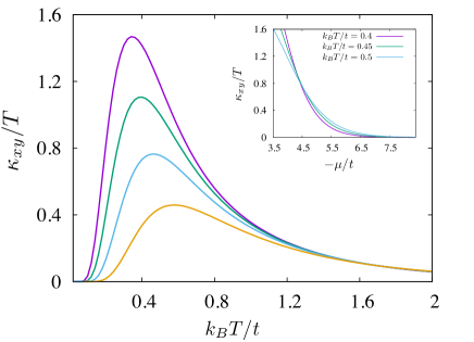
Figure 6: (Color online.) The “magnetic monopole” thermal Hall coefficient $\kappa_{xy}/T$ versus the temperature $k_{B}T/t$. Curves with different colors (from top to bottom) are plotted with a decreasing sequence of chemical potential ${-\mu/t=4,4.2,4.5,5}$. The thermal Hall coefficient $\kappa_{xy}/T$ is in a unit of $k_{B}^{2}/(2\pi\hbar a)\simeq 2.8\times 10^{-4}$ W/(K²m). Inset: The thermal hall coefficient $\kappa_{xy}/T$ is plotted versus the chemical potential $-\mu/t$ for a set of temperatures.

IV.4 Topological thermal Hall effect in weak external field limit

The TTHE is related to the Berry curvature of “magnetic monopole” bands that arise from the induced dual U(1) gauge flux. Under generic magnetic fields, the flux is incommensurate, and diagonalizing the monopole Hamiltonian in presence of arbitrary gauge flux constitutes a 3D Hofstadter problem Hofstadter (1976); Chen (2017a). The incommensurability merely brings some calculational complexity, but our formalism should be readily extended over there and the calculation can be performed numerically.

To demonstrate the usefulness of our theory in the generic commensurate flux cases, we calculate the thermal Hall coefficient along the same external field direction $\hat{n}=\langle 0\bar{1}\bar{1}\rangle$ with the field strength,

$$H_{0}/U=\frac{\sqrt{3}}{\sqrt{2}}\frac{p}{2q},\ \ p,q\in{\cal Z}$$ (33)

where $p,q$ are integer numbers, and the external field strength is proportional to a gauge flux ratio $p/2q$. The gauge flux on the diamond hexagon takes a form,

$$2\pi\ {\rm curl}\,a^{0}_{r,r+e_{\mu}}=\left\{\begin{array}[]{cc}\pi-(p/q)\pi,&\ \ \ \ \ \mu=0,\\ \pi+(p/q)\pi,&\ \ \ \ \ \mu=1,\\ \pi+0,&\ \ \ \ \ \mu=2,\\ \pi+0,&\ \ \ \ \ \mu=3.\\ \end{array}\right.$$ (34)

Accordingly, the gauge fixing condition on the dual diamond lattice is given by,

$$2\pi a^{0}_{\textsf{r},\textsf{r}+e_{\mu}}= \xi_{\mu}({\bf q}_{1}\cdot\textsf{r})+\eta_{\mu}({\bf q}_{2}\cdot\textsf{r}),\ \ \ \textsf{r}\in{\rm I},$$ (35)

$${\bf q}_{1}= 2\pi(100),\ \xi_{\mu}=(1001),$$

$${\bf q}_{2}= (p/q)2\pi(100),\ \eta_{\mu}=(0001).$$

The case we demonstrated in Sec. IV.2 is regarded as a special case with $p=1,q=2$. For the general integer values of $(p,q)$, the magnetic unit-cell is enlarged along the $a_{2}$-direction in Fig. 3, constituting $4q$ number of distinct dual diamond sites. With the gauge fixing condition for generic commensurate flux, we estimate the TTHE under various external field strength. We plot the thermal Hall coefficient $\kappa_{xy}/T$ versus the gauge flux ratio $p/2q$ in Fig. 7 for three representative temperature points. The thermal Hall coefficient admits a primitive zone of gauge flux ratio $p/2q\in[-0.5,0.5)$, and is periodic with respect to the shift of integer gauge flux ratio. At the zone center and boundary $p/2q=0,-0.5$, the TTHE is absent due to the preservation of the time reversal symmetry. The magnitude of the thermal Hall coefficient $\kappa_{xy}$ increases along with the ratio $p/2q\in[0,0.5)$, and changes sign when the external field direction is reversed $p/2q\in[-0.5,0)$. The finite value of thermal Hall coefficient indicates that the TTHE is no fluke under the specific gauge choice, rather, it is a universal phenomenon in the presence of generic commensurate flux.

For the incommensurate flux case at arbitrary field strength, we can approximate the incommensurate flux to a nearby commensurate one in the weak field limit. The weak field limit is consistent with our previous assumption, which guarantees the existence of the underlying QSL ground state. Furthermore, we have considered a semiclassical version of the “monopole” thermal Hall effect under generic magnetic fields and develop a continuous theory for this effect. This will be explained in a future work.

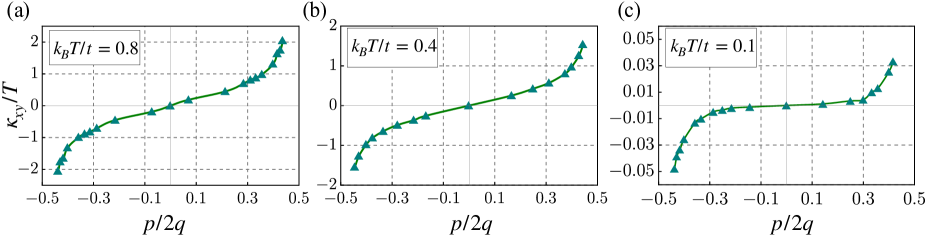
Figure 7: The “magnetic monopole” thermal Hall coefficient $\kappa_{xy}/T$ versus the field strength ratio $p/2q$ for various temperature: (a) $k_{B}T/t=0.8$, (b) $k_{B}T/t=0.4$, (c) $k_{B}T/t=0.1$. The chemical potential is fixed at $-\mu/t=4$. $\kappa_{xy}/T$ is in a unit of $k_{B}^{2}/(2\pi\hbar a)\simeq 2.8\times 10^{-4}$ W/(K²m).

V Discussion

To summarize, we made the observation from the electromagnetic duality that, the external magnetic field could generate emergent electric field distribution and thus the dual U(1) gauge flux for the “magnetic monopoles”. We developed a formalism to calculate the modulation of the monopole band structure and the monopole Berry curvature, and explained the physical origin of the monopole thermal Hall effects. To provide an illuminating discussion of the implication and underlying insights of our results, we first make a comparison between our current theory for the pyrochlore U(1) QSL and other U(1) QSLs. Then, we will focus on the pyrochlore magnets and make a materials’ survey about the thermal Hall effects among the pyrochlore U(1) QSL candidate materials.

V.1 Comparison with other U(1) QSLs in both weak and strong Mott regimes

Thermal Hall effect was suggested for the spinon Fermi surface U(1) QSLs in the weak Mott regime. This effect is actually quite natural in the weak Mott regime Motrunich (2006); Katsura et al. (2010). Over there, the concept of spinons are not so distinct from the physical electrons due to the weak Mott gap and strong charge fluctuations. Physically, this can be understood from the fact that the external gauge flux enters into the four-spin ring exchange interaction Sen and Chitra (1995); Motrunich (2006). From the gauge theory description, the internal U(1) gauge flux is locked to the external U(1) gauge flux through the strong charge fluctuations, such that the spinon motion is twisted by the induced internal U(1) gauge flux. Similar ideas have been extended to the mixed valence compounds where the Fermi surface of neutral particles has been proposed Chowdhury et al. (2018), although the thermal Hall measurement in SmB₆ or YbB₁₂ gives a zero result Matsuda . For strong Mott insulators, the charge gap is large and the charge fluctuation is strongly suppressed. This induction of the internal U(1) gauge flux via strong charge fluctuations does not apply to the strong Mott regimes.

In the U(1) QSLs in the strong Mott regime, different physical mechanisms are needed to understand the large thermal Hall effect. For the U(1) QSLs whose gauge flux is related to the scalar spin chirality ${({\bm{S}}_{i}\times{\bm{S}}_{j})\cdot{\bm{S}}_{k}}$, we pointed out that, the combination of the Dzyaloshinskii-Moriya interaction and a simple Zeeman coupling could generate an internal U(1) gauge flux, and thus twist the motion of the spinons Yong Hao Gao and Gang Chen (2019); Gao et al. (2019). This mechanism does not depend on the choices of the (bosonic) Schwinger spinons or the (fermionic) Abrikosov spinons. The (fermionic) Abrikosov spinons describe more QSL states in 2D. The bosonic Schwinger spinon does not work for U(1) QSLs in 2D due to the confinement issue from the instanton effect. So for the Schwinger spinon description, this mechanism would only apply to the 3D U(1) QSL. In contrast, this mechanism broadly applies to the U(1) QSLs with the fermionic spinon description.

For the pyrochlore U(1) QSL that is also in the strong Mott regime, the relation of the internal variable and the physical variable is much simpler than the one described in the previous paragraph. So the linear Zeeman coupling already induces an internal dual U(1) gauge flux and twist the motion of the “magnetic monopoles.”

In general, for the QSLs with a continuous gauge theory description, one key to resolve the mechanism for the thermal Hall effect is to understand the physical manifestation of the internal gauge flux and then the role of the external probes. This is related to the relation between the microscopic degrees of freedom and the emergent degrees of freedom in the lattice gauge theory formulation.

V.2 Comparison with $\mathbb{Z}_{2}$ QSLs

For $\mathbb{Z}_{2}$ QSLs, the above mechanism does not apply because the internal gauge flux is gapped and discrete and cannot be changed in a continuous manner. An example would be the $\mathbb{Z}_{2}$ QSL from the Balents-Fisher-Girvin model Balents et al. (2002). Although the $\mathbb{Z}_{2}$ vison experiences a dual background $\pi$ flux and the $S^{z}$-$S^{z}$ dynamical correlation has a spectral periodicity enhancement, a small magnetic field cannot modify this background flux continuously. Likewise, the spinons experience a background $0$ flux, and the magnetic field cannot change this flux continuously. Thus the mechanism in the previous subsection neither applies to the spinon nor to the vison. In $\mathbb{Z}_{2}$ QSLs, instead, it is the non-trivial band structure of matter field that directly contributes to the thermal Hall conductivity. A representative example would be the Kitaev model at the isotropic point where the spinons develop a gapless Dirac-type majorana ferminon band structure Kitaev (2006). When the magnetic field is applied to the system, the field generates a mass gap for the majorana fermions and creates a topological spinon band structure with a non-trivial Chern number. This is the origin of the thermal Hall effect for Kitaev QSL.

Another studied case Rhine Samajdar, Shubhayu Chatterjee, Subir Sachdev, and Mathias S. Scheurer (2018) are gapped $\mathbb{Z}_{2}$ QSLs with the Schwinger boson description. The Dzyaloshinskii-Moriya interaction and the Zeeman coupling together breaks the time reversal symmetry and inversion symmetry. It was suggested that, using the Schwinger boson construction, the Dzyaloshinskii-Moriya interaction and the Zeeman coupling together generates a non-trivial Berry curvature distribution for the (gapped) bosonic spinon bands. At finite temperatures, the spinon bands are populated thermally, contributing to the thermal Hall conductivity.

V.3 Materials’ survey

The pyrochlore U(1) QSLs have been proposed for several rare-earth pyrochlore magnets. Here we give a detailed discussion about the potential thermal Hall conductivity in some key representatives.

We start with the non-Kramers doublets. Here the Tb family Tb₂Ti₂O₇ Molavian et al. (2007); Kermarrec et al. (2015); Taniguchi et al. (2013) and the Pr family (Pr₂Zr₂O₇, Pr₂Sn₂O₇, Pr₂Hf₂O₇) Kimura et al. (2013); Sibille et al. (2018a); Princep et al. (2013) have been proposed as pyrochlore U(1) QSLs. The thermal Hall effect has been measured in Tb₂Ti₂O₇ Hirschberger et al. (2015), and inelastic neutron scattering measurement has been performed on the Pr-based family Wen et al. (2017); Savary and Balents (2017b); Sibille et al. (2018b). The continuous spectrum has been obtained experimentally. It was proposed that, the inelastic neutron scattering results for the non-Kramers doublets would contain the continuum of the “magnetic monopoles” from the duality arguments Chen (2017a). Other theory from the crystal field disorders of the non-Kramers doublets interpreted the excitation continuum differently Savary and Balents (2017b). The Tb₂Ti₂O₇ sample can become Ising ordered once the stoichiometry of the sample is changed Taniguchi et al. (2013); Kermarrec et al. (2015). Actually since Tb³⁺ carries a non-Kramers doublet, the Ising order transition should be understood as the “magnetic monopole” condensation out of the U(1) QSL if the original disordered state is a U(1) QSL Chen (2016). Therefore, both Tb-based and Pr-based rare-earth pyrochlore materials can be good candidates for the pyrochlore U(1) QSLs. We expect a non-trivial thermal Hall effect to be established in these candidate materials.

The well-known Yb₂Ti₂O₇ Yan et al. (2017); Ross et al. (2009); Thompson et al. (2017); Jaubert et al. (2015); Applegate et al. (2012); Arpino et al. (2017); Pe çanha Antonio et al. (2017); Robert et al. (2015); Bowman et al. (2019) is now under debate Ross et al. (2011). Here the Yb³⁺ ion is a Kramers ion and differs from the non-Kramers Pr³⁺ ion. The actual low-temperature phase depends sensitively on the preparation of the samples. For the physical point of view, it does not really matter strongly whether the magnetic ordered state of the system is proximate to the spin ice or not proximate to spin ice. The pyrochlore U(1) QSL can persist beyond the perturbative spin ice regime. A more sensible question would be whether Yb₂Ti₂O₇ is proximate to the pyrochlore U(1) QSL rather than proximate to the (perturbative) spin ice manifold. If the system is proximate to the pyrochlore U(1) QSL, then TTHE of “magnetic monopoles” could be relevant and may even persist to the weak ordered regime, despite the fact that the Zeeman coupling involves the transverse spin components. The Zeeman coupling with the transverse spin components modifies the spinon dispersion and could provide a thermal Hall signal of spinons. As the spinons usually have much higher energy scales than the “magnetic monopoles”, we expect that the low-temperature thermal Hall effect is still dominated by the “magnetic monopoles”.

Recently, Ce₂Zr₂O₇, Ce₂Sn₂O₇, and Ce₂Hf₂O₇ have been realized and proposed as QSLs Sibille et al. (2015); Gao et al. (2019). The Ce³⁺ ion is also a Kramers ion of the dipole-octupole type Huang et al. (2014), but differs from the Yb³⁺ ion. Each state of the ground state doublet of the Ce³⁺ ion is a one-dimensional irreducible representation of the D_3d point group Li and Chen (2017a); Yao-Dong Li and Gang Chen (2019), while the two states of the Yb³⁺ ion comprise a two-dimensional irreducible representation. It was suggested that, two distinct symmetry enriched U(1) QSLs, i.e., dipolar U(1) QSL and octupolar U(1) QSL, can be stabilized by studying the generic model for dipole-octupole doublets. The dipolar U(1) QSL is identical to the one obtained for the non-Kramers doublets and the usual Kramers doublets. Since the external magnetic field primarily couples to the dipolar component at the linear level, if the dipolar U(1) QSL is stabilized, then we expect the TTHE of “magnetic monopoles.” On the other hand, if the octupolar U(1) QSL is stabilized, the external magnetic field would modify the spinon band structure Li and Chen (2017a); Yao-Dong Li and Gang Chen (2019) but would not change the dual U(1) flux for the “magnetic monopoles,” so we do not expect the TTHE for the “magnetic monopoles.”

VI Acknowledgments

We acknowledge Xuefeng Sun from USTC for the discussion of experimental setups. XTZ acknowledges Ryuichi Shindou for previous collaborations on the duality related topics. This work is supported by the Ministry of Science and Technology of China with Grant No.2016YFA0301001, 2016YFA0300500, 2018YFGH000095 and by General Research Fund (GRF) No.17303819 from the Research Grants Council of Hong Kong.

Appendix A Duality transformation

Start from the ring exchange Hamiltonian in Eq. (2), we rewrite in terms of a particle number $n_{i}$ (integer-valued) and a conjugated phase $\phi_{i}$ ,

$$\tau^{\pm}_{i}=e^{\pm i\phi_{i}}$$ (36)

$$\tau^{z}_{i}=n_{i}-\frac{1}{2}$$

which satisfy the commutation relation

$$[\phi_{i},n_{i}]=i$$ (37)

Moreover, $\tau^{z}_{i}$ takes the eigenvalue of $\pm 1/2$. To ensure the Hilbert space is not enlarged, we add a constrain term $(n_{i}-\frac{1}{2})^{2}$ with a strength $U$. The particle number takes values $n_{i}=0,1$, and, we obtain a Hamiltonian

$${\cal H}_{\rm ring}= -K\sum_{\hexagon_{p}}\cos\big{(}\phi_{1}-\phi_{2}+\phi_{3}-\phi_{4}+\phi_{5}-\phi_{6}\big{)}$$ (38)

$$+\frac{U}{2}\sum_{i}(n_{i}-\frac{1}{2})^{2}$$

Now, we transform to the electric field and gauge field, which are defined on the diamond lattice, (see Fig. 2)

$$A_{rr^{\prime}}=\epsilon_{r}\phi_{rr^{\prime}}$$ (39)

$$E_{rr^{\prime}}=\epsilon_{r}n_{rr^{\prime}}$$

where the pyrochlore site $i$ sits in the middle of the link $rr^{\prime}$. $\epsilon_{r}=+1(-1)$ for diamond lattice type-${\rm I}({\rm II})$. Thus, the variables are anti-symmetric ${\cal G}_{r^{\prime}r}=-{\cal G}_{rr^{\prime}},\ \ {\cal G}=A,E$. And, the commutation relation follows from Eq. (37)

$$[A_{rr^{\prime}},E_{rr^{\prime}}]=\epsilon_{r}^{2}[\phi_{i},n_{i}]=i$$ (40)

We fix the branch-cut for the $2\pi$-periodic variable as $A_{rr^{\prime}}\in[-\pi,+\pi)$, so that a lattice curl of this variable remains non-vanishing,

$${\rm curl}A(\textsf{r}\textsf{r}^{\prime})=\sum_{rr^{\prime}\in\hexagon_{d(\textsf{r}\textsf{r}^{\prime})}}A_{rr^{\prime}}$$ (41)

where the original diamond hexagon $\hexagon_{d(\textsf{r}\textsf{r}^{\prime})}$ is labelled by the dual diamond link $\textsf{r}\textsf{r}^{\prime}$ that penetrates the hexagon. The phase terms in Eq. (38) is expressed in an elegant way,

$${\cal H}_{\rm LGT}[A,E]= -K\sum_{\hexagon_{d(\textsf{r}\textsf{r}^{\prime})}}\cos({\rm curl}A_{\textsf{r}\textsf{r}^{\prime}})$$ (42)

$$+\frac{U}{2}\sum_{rr^{\prime}}\big{(}E_{rr^{\prime}}-\frac{\epsilon_{r}}{2}\big{)}^{2}$$

which has been presented in Eq. (3) as a lattice gauge theory. And, the corresponding action reads,

$${\cal S}_{\rm LGT}[A,E]= \sum_{rr^{\prime}}A_{rr^{\prime}}\partial_{t}E_{rr^{\prime}}+{\cal H}_{\rm LGT}[A,E]$$ (43)

Along this line of derivation, we should keep track of a “2-in-2-out” configuration of the spins in a pyrochlore tetrahedra,

$$\sum_{i\in{\rm teh}_{r}}\tau^{z}_{i}=0$$ (44)

where pyrochlore sites $i$ belong to the tetrahedra labelled by its center $r$-site. As a result, the electric field is imposed with a constraint

$${\rm div}E(r)\equiv\sum_{r^{\prime}\in r}E_{rr^{\prime}}=\sum_{i\in r}n_{i}=2\epsilon_{r}$$ (45)

where the summation defines a lattice divergence, and $r^{\prime}\in r$ refers to the four nearest neighbor original site of a given original site $r$.

Next, we transform the LGT to a dual theory by defining

$${\rm curl}a_{rr^{\prime}}=E_{rr^{\prime}}-E^{0}_{rr^{\prime}}$$ (46)

$$B_{\textsf{r}\textsf{r}^{\prime}}={\rm curl}A_{\textsf{r}\textsf{r}^{\prime}}$$

where a magnetic field $a_{\textsf{r}\textsf{r}^{\prime}}$ (integer-valued) and dual gauge field $B_{\textsf{r}\textsf{r}^{\prime}}$ ($2\pi$-periodic). The curl of the dual gauge field is related to the electric field, therefore the z-component spin. It is valid for a gauge invariant quantity to represent a physical one. Since the dual gauge field is integer-valued, we expect no divergence for its lattice curve. On the other hand, as dictated in Eq. (45), the electric field has a non-vanishing divergence. A background electric field is introduced to ensure the divergencelessness of the dual gauge field. We pick a particular configuration within the 2-in-2-out spin ice manifold,

$$E^{0}_{r,r+\epsilon_{r}e_{0}}= E^{0}_{r,r+\epsilon_{r}e_{1}}=\epsilon_{r}$$ (47)

$$E^{0}_{r,r+\epsilon_{r}e_{2}}= E^{0}_{r,r+\epsilon_{r}e_{3}}=0$$

The dual lattice gauge theory is written as,

$${\cal H}_{\rm dual}[a,B]= \sum_{rr^{\prime}}\frac{U}{2}({\rm curl}\ a_{rr^{\prime}}-\bar{E}_{rr^{\prime}})^{2}-K\sum_{\textsf{r}\textsf{r}^{\prime}}\cos B_{\textsf{r}\textsf{r}^{\prime}}$$ (48)

where the background electric field is defined in Eq. (7). The corresponding action follows from Eq. (43)

$${\cal S}_{\rm dual}[a,B]= \sum_{rr^{\prime}}A_{rr^{\prime}}\partial_{t}({\rm curl}\ a_{rr^{\prime}}+{E}^{0}_{rr^{\prime}})+{\cal H}_{\rm dual}[a,B]$$ (49)

$$= \sum_{\textsf{r}\textsf{r}^{\prime}}B_{\textsf{r}\textsf{r}^{\prime}}\partial_{t}(a_{\textsf{r}\textsf{r}^{\prime}}+a^{0}_{\textsf{r}\textsf{r}^{\prime}})+{\cal H}_{\rm dual}[a,B]$$

where $a^{0}_{\textsf{r}\textsf{r}^{\prime}}$ is the vector potential responsible for the electric field ${E}^{0}_{rr^{\prime}}={\rm curl}a^{0}_{rr^{\prime}}$. And, in the second equality we have exchanged the sequence of the summation over original and dual lattices,

$$\sum_{rr^{\prime}}\sum_{\textsf{r}\textsf{r}^{\prime}\in\hexagon^{\ast}_{d(rr^{\prime})}}=\sum_{\textsf{r}\textsf{r}^{\prime}}\sum_{rr^{\prime}\in\hexagon_{d(\textsf{r}\textsf{r}^{\prime})}}$$ (50)

The divergence of the magnetic field is non-zero by definition

$${\rm div}B_{\textsf{r}}\equiv {\rm div}\cdot{\rm curl}A(\textsf{r})$$ (51)

$$= \sum_{\textsf{r}^{\prime}\in\textsf{r}}\sum_{rr^{\prime}\in\hexagon_{d(\textsf{r}\textsf{r}^{\prime})}}{A_{rr^{\prime}}}_{[-\pi,\pi)}$$

$$= 2\pi{\cal Z}$$

The “magnetic monopole” number operator is defined as the topological defect of this magnetic field,

$$N_{\textsf{r}}\equiv\frac{1}{2\pi}{\rm div}B_{\textsf{r}}$$ (52)

which takes integer values. The commutation relation between the dual variables can be derived from Eq. (40),

$$\big{[}\sum_{rr^{\prime}\in\hexagon_{d(\textsf{r}\textsf{r}^{\prime})}}A_{rr^{\prime}},E_{rr^{\prime}}\big{]}=i$$ (53)

so that, we have

$$\big{[}B_{\textsf{r}\textsf{r}^{\prime}},\sum_{\textsf{r}_{1}\textsf{r}^{\prime}_{1}\in\hexagon^{\ast}_{d(rr^{\prime})}}a_{\textsf{r}_{1}\textsf{r}_{1}^{\prime}}\big{]}=i,\ \ \ \textsf{r}\textsf{r}^{\prime}\in\hexagon^{\ast}_{d(rr^{\prime})}$$ (54)

Particularly, we can make a convenient choice

$$\big{[}B_{\textsf{r}\textsf{r}^{\prime}},a_{\textsf{r}_{1}\textsf{r}_{1}^{\prime}}\big{]}=\left\{\begin{array}[]{cc}i,&\ \ \ \ \ \textsf{r}_{1}\textsf{r}_{1}^{\prime}=\textsf{r}\textsf{r}^{\prime}\\ 0,&\ \ \ \ \ \textsf{r}_{1}\textsf{r}_{1}^{\prime}\neq\textsf{r}\textsf{r}^{\prime}\\ \end{array}\right.$$ (55)

which we have used in and below Eq. (5). Finally, we note that the two dual variables are anti-symmetric with respect to exchanging the lattice sites. This fact follows from the definitions in Eq. (39) and Eq. (46).

From Eq.(51) and Eq.(52), we see that the “magnetic monopole” is the topological defect of the dual vector gauge potential in the compact U(1) quantum electrodynamics and has no classical analog. Even though the spinon and the “magnetic monopole” can be interchanged by the electromagnetic duality of the lattice gauge theory, the “magnetic monopole” might be more close in spirit to Dirac’s magnetic monopole from the original definition and theory of the pyrochlore U(1) QSLHermele et al. (2004).

So far, we have derived the dual gauge theory. The commutation relation of variables is properly kept along the way. And, we have identified the “magnetic monopole” number operator, however, a conjugated phase operator of the “magnetic monopole” is missing in the present formulation. Moreover, the dual gauge field is a discretized variable, which is cumbersome to deal with in terms of standard field theory methods. Fortunately, during the process of “softening” the dual gauge field, we can introduce the phase operator of the “magnetic monopole” in a natural way. And, we are able to establish a commutation relation between the introduced phase variable and the “magnetic monopole” number operator.

Appendix B “Variable-soften” procedure

The model describes a confinement-deconfinement phase transition due to the discreteness of the dual U(1) gauge field. Otherwise, the partition function is basically a trivial Gaussian model. Let us consider the dual gauge field part of the partition function,

$$Z[a]\equiv \sum_{\{a_{\textsf{r}\textsf{r}^{\prime}}\}}e^{-\sum_{rr^{\prime}}\frac{U}{2}({\rm curl}\ a_{rr^{\prime}}-\bar{E}_{rr^{\prime}})^{2}}$$ (56)

$$= \int{\mathcal{D}}{a}\sum_{\{{p}_{rr^{\prime}}\}}\ e^{-\sum_{rr^{\prime}}\frac{U}{2}({\rm curl}\ a_{rr^{\prime}}-\bar{E}_{rr^{\prime}})^{2}}$$

$$\times e^{i2\pi\sum_{rr^{\prime}}{\rm curl}\ a_{rr^{\prime}}\cdot p_{rr^{\prime}}}$$

where we have the used the Poisson’s resummation rule to leverage the discreteness of $a_{\textsf{r}\textsf{r}^{\prime}}$,

$$\sum_{m=-\infty}^{+\infty}e^{i2\pi mx}=\sum_{n=-\infty}^{+\infty}\delta(x-n)$$ (57)

We can further transform the expression

$$Z[a]= \int{\mathcal{D}}{a}\sum_{\{{p}_{rr^{\prime}}\}}\ e^{-\sum_{rr^{\prime}}\frac{U}{2}({\rm curl}\ a_{rr^{\prime}}-\bar{E}_{rr^{\prime}})^{2}}$$ (58)

$$\times e^{i2\pi\sum_{\textsf{r}\textsf{r}^{\prime}}a_{\textsf{r}\textsf{r}^{\prime}}\cdot{\rm curl}\ p_{\textsf{r}\textsf{r}^{\prime}}}$$

by manipulating the two summations involved,

$$\sum_{rr^{\prime}}{\rm curl}a_{rr^{\prime}}\cdot p_{rr^{\prime}}= \sum_{rr^{\prime}}\sum_{\textsf{r}\textsf{r}^{\prime}\in\hexagon^{\ast}_{d(rr^{\prime})}}a_{\textsf{r}\textsf{r}^{\prime}}\cdot p_{rr^{\prime}}$$ (59)

$$= \sum_{\textsf{r}\textsf{r}^{\prime}}\sum_{rr^{\prime}\in\hexagon_{d(\textsf{r}\textsf{r}^{\prime})}}a_{\textsf{r}\textsf{r}^{\prime}}\cdot p_{rr^{\prime}}$$

$$= \sum_{\textsf{r}\textsf{r}^{\prime}}a_{\textsf{r}\textsf{r}^{\prime}}\cdot{\rm curl}\ p_{\textsf{r}\textsf{r}^{\prime}}$$

Importantly, the dual gauge field is anti-symmetric, i.e., $a_{\textsf{r}^{\prime}\textsf{r}}=-a_{\textsf{r}\textsf{r}^{\prime}}$. The curl of the auxiliary field ${\rm curl}\ p_{\textsf{r}\textsf{r}^{\prime}}$ is anti-symmetric as well, so the summation in Eq. (59) gives non-vanishing result. Moreover, this curl is divergentless, since $p_{rr^{\prime}}$ is an integer-valued variable. The divergentless and anti-symmetric properties can be made explicit in the path integral formulation,

$$Z[a]= \int{\mathcal{D}}{a}e^{-\sum_{rr^{\prime}}\frac{U}{2}({\rm curl}\ a_{rr^{\prime}}-\bar{E}_{rr^{\prime}})^{2}}\times\{...\}$$ (60)

$$\{...\}= \sum_{\{{M}^{\rm asym}_{\textsf{r}\textsf{r}^{\prime}}\}}\delta\Big{[}{\rm div}M^{\rm asym}(\textsf{r})\Big{]}\ e^{i2\pi\sum_{\textsf{r}\textsf{r}^{\prime}}a_{\textsf{r}\textsf{r}^{\prime}}\cdot M^{\rm asym}_{\textsf{r}\textsf{r}^{\prime}}}$$

where $M^{\rm asym}_{\textsf{r}\textsf{r}^{\prime}}$ is anti-symmetric, integer-valued variable, and the lattice divergence is ${\rm div}M^{\rm asym}(\textsf{r})=\sum_{\textsf{r}^{\prime}\in\textsf{r}}M^{\rm asym}_{\textsf{r}\textsf{r}^{\prime}}$. The delta function can be removed by introducing another auxiliary field $\theta_{\textsf{r}}$,

$$\{...\}= \sum_{\{{M}^{\rm asym}_{\textsf{r}\textsf{r}^{\prime}}\}}e^{i2\pi\sum_{\textsf{r}\textsf{r}^{\prime}}a_{\textsf{r}\textsf{r}^{\prime}}\cdot M^{\rm asym}_{\textsf{r}\textsf{r}^{\prime}}}\int{\cal D}\theta\ e^{i\sum_{\textsf{r}}{\rm div}M^{\rm asym}_{\textsf{r}}\cdot\theta_{\textsf{r}}}$$ (61)

Now, we are in the position to remove the anti-symmetric condition

$$\sum_{\textsf{r}}{\rm div}M^{\rm asym}_{\textsf{r}}\cdot\theta_{\textsf{r}}= \sum_{\textsf{r}}\sum_{\textsf{r}^{\prime}\in\textsf{r}}M^{\rm asym}_{\textsf{r}\textsf{r}^{\prime}}\cdot\theta_{\textsf{r}}$$ (62)

$$= \sum_{\textsf{r}\textsf{r}^{\prime}}(M_{\textsf{r}\textsf{r}^{\prime}}-M_{\textsf{r}^{\prime}\textsf{r}})\theta_{\textsf{r}}$$

$$= \sum_{\textsf{r}\textsf{r}^{\prime}}M_{\textsf{r}\textsf{r}^{\prime}}(\theta_{\textsf{r}}-\theta_{\textsf{r}^{\prime}})$$

So that, we arrive at an elegant expression, which is similar to the result in literature Herbut (2007)

$$\{...\}= \sum_{\{{M}_{\textsf{r}\textsf{r}^{\prime}}\}}e^{i2\pi\sum_{\textsf{r}\textsf{r}^{\prime}}a_{\textsf{r}\textsf{r}^{\prime}}\cdot M_{\textsf{r}\textsf{r}^{\prime}}}e^{i\sum_{\textsf{r}\textsf{r}^{\prime}}M_{\textsf{r}\textsf{r}^{\prime}}(\theta_{\textsf{r}}-\theta_{\textsf{r}^{\prime}})}$$ (63)

Following the series of transformation and perform a Villain approximation, we end up with the dual theory in Eq. (1). The

$${\cal H}_{\rm dual}[\theta,a,B]= \sum_{rr^{\prime}}\frac{U}{2}({\rm curl}\ a_{rr^{\prime}}-\bar{E}_{rr^{\prime}})^{2}-\sum_{\textsf{r}\textsf{r}^{\prime}}K\cos B_{\textsf{r}\textsf{r}^{\prime}}$$ (64)

$$-t\sum_{\textsf{r}\textsf{r}^{\prime}}\cos(\theta_{\textsf{r}}-\theta_{\textsf{r}^{\prime}}+2\pi a_{\textsf{r}\textsf{r}^{\prime}})$$

$${\rm cond}: {\rm div}B(\textsf{r})=2\pi N_{\textsf{r}}$$

where a parameter $t$ is added as a chemical potential term for the $M_{\textsf{r}\textsf{r}^{\prime}}$. So far, we have resolve the discreteness issue of the dual gauge field by introducing a phase field $\theta_{\textsf{r}}$. At the moment, the physical meaning of this variable is not clear, namely, the commutation relation with the other variables are not given.

Further progress is made by manipulating the condition in Eq. (64). The full partition function and action are given by,

$$Z= \int{\mathcal{D}}\theta{\mathcal{D}}a\int_{\rm cond}{\mathcal{D}}Be^{i\sum_{\textsf{r}\textsf{r}^{\prime}}B_{\textsf{r}\textsf{r}^{\prime}}\partial_{\tau}(a_{\textsf{r}\textsf{r}^{\prime}}+a^{0}_{\textsf{r}\textsf{r}^{\prime}})-{\cal H}_{\rm dual}[\theta,a,B]}$$ (65)

$$\equiv \int{\mathcal{D}}\theta{\mathcal{D}}a\int_{\rm cond}{\mathcal{D}}Be^{-{\cal S}_{\rm dual}[\theta,a,B]}$$

where the condition in the integral can be made explicit by inserting another delta function,

$$Z= \int{\mathcal{D}}\theta{\mathcal{D}}a\int{\mathcal{D}}B\delta\big{[}{\rm div}B(\textsf{r})-2\pi N_{\textsf{r}}\big{]}e^{-{\cal S}_{\rm dual}[\theta,a,B]}$$ (66)

$$= \int{\mathcal{D}}\theta{\mathcal{D}}a{\mathcal{D}}B{\mathcal{D}}\Lambda\ e^{i\sum_{\textsf{r}}\Lambda_{\textsf{r}}({\rm div}B_{\textsf{r}}-2\pi N_{\textsf{r}})}e^{-{\cal S}_{\rm dual}[\theta,a,B]}$$

where $G(\Lambda)=e^{i\sum_{\textsf{r}}\Lambda_{\textsf{r}}({\rm div}B_{\textsf{r}}-2\pi N_{\textsf{r}})}$ is regarded as a gauge fixing generator Fisher (2004), which can be transformed in the similar way as in Eq. (62),

$$G(\Lambda)=e^{i\sum_{\textsf{r}\textsf{r}^{\prime}}B_{\textsf{r}\textsf{r}^{\prime}}(\Lambda_{\textsf{r}}-\Lambda_{\textsf{r}^{\prime}})}e^{-i2\pi\sum_{\textsf{r}}N_{\textsf{r}}\Lambda_{\textsf{r}}}$$ (67)

This function generates a gauge transformation for functions involving the dual gauge field and the phase variable,

$$G(\Lambda){\cal S}_{\rm dual}(a_{\textsf{r}\textsf{r}^{\prime}},\theta_{\textsf{r}},B_{\textsf{r}\textsf{r}^{\prime}})G^{\dagger}(\Lambda)$$ (68)

$$= {\cal S}_{\rm dual}\big{[}a_{\textsf{r}\textsf{r}^{\prime}}+(\Lambda_{\textsf{r}}-\Lambda_{\textsf{r}^{\prime}}),\theta_{\textsf{r}}+2\pi\Lambda_{\textsf{r}},B_{\textsf{r}\textsf{r}^{\prime}}\big{]}$$

under the condition that the following commutation relation is satisfied,

$$[\theta_{\textsf{r}},N_{\textsf{r}^{\prime}}]=i\delta_{\textsf{r},\textsf{r}^{\prime}}$$ (69)

The transformed action is equivalent to the original one by absorbing the field $\Lambda_{\textsf{r}}$, we have

$$Z= \int{\mathcal{D}}\theta{\mathcal{D}}a{\mathcal{D}}B{\mathcal{D}}\Lambda\ e^{-{\cal S}_{\rm dual}[\theta,a,B]}e^{i\sum_{\textsf{r}}\Lambda_{\textsf{r}}({\rm div}B_{\textsf{r}}-2\pi N_{\textsf{r}})}$$ (70)

$$= \int{\mathcal{D}}\theta{\mathcal{D}}a\int{\mathcal{D}}Be^{-{\cal S}_{\rm dual}[\theta,a,B]}\delta\big{[}{\rm div}B(\textsf{r})-2\pi N_{\textsf{r}}\big{]}$$

$$= \int{\mathcal{D}}\theta{\mathcal{D}}a\int_{\rm cond}{\mathcal{D}}Be^{-{\cal S}_{\rm dual}[\theta,a,B]}$$

where the action is intact after applying the gauge generator obeying the commutation rule in Eq. (69). Therefore, the variable $\theta$ admits a physical meaning of the conjugated phase of the magnetic monopole. $e^{i\theta}(e^{-i\theta})$ is the creation(annihilation) operator for the magnetic monopole.

Conclusively, we finish the task of softening the dual gauge field in the dual theory, meanwhile, introducing the magnetic monopole phase variable. We emphasize on the peculiar definition of curl and divergence in the diamond lattice structure, and the anti-symmetric property of the link variables.

Appendix C Thermal Hall Current Operator

In Sec. III, we present the result for the thermal Hall current at the mean-field level. Here, we derive a compact expression for the thermal Hall current in the presence of gauge fluctuation. We start from the same energy continuity equation as in Eq. (15), yet with a different energy density operator,

$${\cal H}_{\rm dual}= \sum_{\textsf{r}}{\cal H}_{\textsf{r}}$$ (71)

$${\cal H}_{\textsf{r}}= \sum_{\textsf{r}^{\prime}\in\textsf{r}}\Big{\{}\frac{U}{2}\sum_{rr^{\prime}\in\hexagon_{d(\textsf{r}\textsf{r}^{\prime})}}({\rm curl}\ a_{rr^{\prime}}-\bar{E}_{rr^{\prime}})^{2}-\frac{K}{2}B_{\textsf{r}\textsf{r}^{\prime}}^{2}$$

$$-\frac{t}{2}e^{i(\theta_{\textsf{r}}-\theta_{\textsf{r}^{\prime}}+2\pi a_{\textsf{r}\textsf{r}^{\prime}})}+{\rm H.c.}\Big{\}}$$

where we have kept the rotor variable $e^{i\theta_{\textsf{r}}}$ instead of the boson field used in the main text. And, the summation of the first term comes from,

$$\sum_{rr^{\prime}}\simeq\sum_{\textsf{r}\textsf{r}^{\prime}}\sum_{rr^{\prime}\in\hexagon_{d(\textsf{r}\textsf{r}^{\prime})}}\simeq\sum_{\textsf{r}}\sum_{\textsf{r}^{\prime}\in\textsf{r}}\sum_{rr^{\prime}\in\hexagon_{d(\textsf{r}\textsf{r}^{\prime})}}$$ (72)

Next, we evaluate the time partial derivative of the energy density

$$\dot{\cal H}_{\textsf{r}}=-i\big{[}{\cal H}_{\textsf{r}},{\cal H}_{\rm dual}\big{]}$$ (73)

$$= i\frac{UK}{4}\sum_{\textsf{r}^{\prime}\in\textsf{r}}\sum_{rr^{\prime}\in\hexagon_{d(\textsf{r}\textsf{r}^{\prime})}}\sum_{\textsf{r}_{1}\textsf{r}^{\prime}_{1}}\big{[}({\rm curl}\ a_{rr^{\prime}}-\bar{E}_{rr^{\prime}})^{2},B^{2}_{\textsf{r}_{1}\textsf{r}^{\prime}_{1}}\big{]}$$

$$+\sum_{\textsf{r}^{\prime}\in\textsf{r}}\sum_{rr^{\prime}}\big{[}B^{2}_{\textsf{r}\textsf{r}^{\prime}},({\rm curl}\ a_{rr^{\prime}}-\bar{E}_{rr^{\prime}})^{2}\big{]}$$

The 1st and 2nd commutators are calculated respectively. In the 1st term, we use the commutation relation in Eq. (54), while in the 2nd term, we use a modified version of commutation relation, i.e., $\big{[}B_{\textsf{r}\textsf{r}^{\prime}},{\rm curl}\ a_{rr^{\prime}}\big{]}=i,\ rr^{\prime}\in\hexagon_{d(\textsf{r}\textsf{r}^{\prime})}$.

$$\{{\rm 1st}\}\equiv \sum_{rr^{\prime}\in\hexagon_{d(\textsf{r}\textsf{r}^{\prime})}}\sum_{\textsf{r}_{1}\textsf{r}^{\prime}_{1}}\big{[}({\rm curl}\ a_{rr^{\prime}}-\bar{E}_{rr^{\prime}})^{2},B^{2}_{\textsf{r}_{1}\textsf{r}^{\prime}_{1}}\big{]}$$ (74)

$$= \sum_{rr^{\prime}\in\hexagon_{d(\textsf{r}\textsf{r}^{\prime})}}\sum_{\textsf{r}_{1}\textsf{r}^{\prime}_{1}}({\rm curl}\ a_{rr^{\prime}}-\bar{E}_{rr^{\prime}})\big{[}{\rm curl}\ a_{rr^{\prime}},B^{2}_{\textsf{r}_{1}\textsf{r}^{\prime}_{1}}\big{]}+\big{[}{\rm curl}\ a_{rr^{\prime}},B^{2}_{\textsf{r}_{1}\textsf{r}^{\prime}_{1}}\big{]}({\rm curl}\ a_{rr^{\prime}}-\bar{E}_{rr^{\prime}})$$

$$= \sum_{rr^{\prime}\in\hexagon_{d(\textsf{r}\textsf{r}^{\prime})}}\sum_{\textsf{r}_{1}\textsf{r}_{1}^{\prime}}\delta[\textsf{r}_{1}\textsf{r}_{1}^{\prime}\in\hexagon^{\ast}_{d(rr^{\prime})}]\Big{\{}({\rm curl}\ a_{rr^{\prime}}-\bar{E}_{rr^{\prime}})(-2iB_{\textsf{r}_{1}\textsf{r}^{\prime}_{1}})+(-2iB_{\textsf{r}_{1}\textsf{r}^{\prime}_{1}})({\rm curl}\ a_{rr^{\prime}}-\bar{E}_{rr^{\prime}})\Big{\}}$$

$$= \sum_{rr^{\prime}\in\hexagon_{d(\textsf{r}\textsf{r}^{\prime})}}\sum_{\textsf{r}_{1}\textsf{r}_{1}^{\prime}\in\hexagon^{\ast}_{d(rr^{\prime})}}({\rm curl}\ a_{rr^{\prime}}-\bar{E}_{rr^{\prime}})(-2iB_{\textsf{r}_{1}\textsf{r}^{\prime}_{1}})+(-2iB_{\textsf{r}_{1}\textsf{r}^{\prime}_{1}})({\rm curl}\ a_{rr^{\prime}}-\bar{E}_{rr^{\prime}})$$

$$= -2i\sum_{rr^{\prime}\in\hexagon_{d(\textsf{r}\textsf{r}^{\prime})}}({\rm curl}\ a_{rr^{\prime}}-\bar{E}_{rr^{\prime}}){\rm curl}\ B_{rr^{\prime}}+{\rm curl}\ B_{rr^{\prime}}({\rm curl}\ a_{rr^{\prime}}-\bar{E}_{rr^{\prime}})$$

$$\{{\rm 2nd}\}\equiv \sum_{\textsf{r}_{1}\textsf{r}_{1}^{\prime}}\sum_{rr^{\prime}\in\hexagon_{d(\textsf{r}_{1}\textsf{r}_{1}^{\prime})}}\big{[}B^{2}_{\textsf{r}\textsf{r}^{\prime}},({\rm curl}\ a_{rr^{\prime}}-\bar{E}_{rr^{\prime}})^{2}\big{]}$$ (75)

$$= \sum_{\textsf{r}_{1}\textsf{r}_{1}^{\prime}}\sum_{rr^{\prime}\in\hexagon_{d(\textsf{r}_{1}\textsf{r}_{1}^{\prime})}}\big{[}B^{2}_{\textsf{r}\textsf{r}^{\prime}},{\rm curl}\ a_{rr^{\prime}}\big{]}({\rm curl}\ a_{rr^{\prime}}-\bar{E}_{rr^{\prime}})+({\rm curl}\ a_{rr^{\prime}}-\bar{E}_{rr^{\prime}})\big{[}B^{2}_{\textsf{r}\textsf{r}^{\prime}},{\rm curl}\ a_{rr^{\prime}}\big{]}$$

$$= \sum_{\textsf{r}_{1}\textsf{r}_{1}^{\prime}}\sum_{rr^{\prime}\in\hexagon_{d(\textsf{r}_{1}\textsf{r}_{1}^{\prime})}}\delta[rr^{\prime}\in\hexagon_{d(\textsf{r}\textsf{r}^{\prime})}]\Big{\{}(2iB_{\textsf{r}\textsf{r}^{\prime}})({\rm curl}\ a_{rr^{\prime}}-\bar{E}_{rr^{\prime}})+({\rm curl}\ a_{rr^{\prime}}-\bar{E}_{rr^{\prime}})(2iB_{\textsf{r}\textsf{r}^{\prime}})\Big{\}}$$

$$= \sum_{\textsf{r}_{1}\textsf{r}_{1}^{\prime}}\sum_{rr^{\prime}}\delta[rr^{\prime}\in\hexagon_{d(\textsf{r}_{1}\textsf{r}_{1}^{\prime})}]\delta[rr^{\prime}\in\hexagon_{d(\textsf{r}\textsf{r}^{\prime})}]\Big{\{}(2iB_{\textsf{r}\textsf{r}^{\prime}})({\rm curl}\ a_{rr^{\prime}}-\bar{E}_{rr^{\prime}})+({\rm curl}\ a_{rr^{\prime}}-\bar{E}_{rr^{\prime}})(2iB_{\textsf{r}\textsf{r}^{\prime}})\Big{\}}$$

$$= \sum_{rr^{\prime}}\delta[rr^{\prime}\in\hexagon_{d(\textsf{r}\textsf{r}^{\prime})}]\sum_{\textsf{r}_{1}\textsf{r}_{1}^{\prime}}\delta[\textsf{r}_{1}\textsf{r}_{1}^{\prime}\in\hexagon^{\ast}_{d(rr^{\prime})}]\Big{\{}......\Big{\}}$$

$$= \sum_{rr^{\prime}\in\hexagon_{d(\textsf{r}\textsf{r}^{\prime})}}\sum_{\textsf{r}_{1}\textsf{r}_{1}^{\prime}\in\hexagon^{\ast}_{d(rr^{\prime})}}\Big{\{}......\Big{\}}$$

$$= 2i\sum_{rr^{\prime}\in\hexagon_{d(\textsf{r}\textsf{r}^{\prime})}}\sum_{\textsf{r}_{1}\textsf{r}_{1}^{\prime}\in\hexagon^{\ast}_{d(rr^{\prime})}}B_{\textsf{r}\textsf{r}^{\prime}}({\rm curl}\ a_{rr^{\prime}}-\bar{E}_{rr^{\prime}})+({\rm curl}\ a_{rr^{\prime}}-\bar{E}_{rr^{\prime}})\sum_{\textsf{r}_{1}\textsf{r}_{1}^{\prime}\in\hexagon^{\ast}_{d(rr^{\prime})}}B_{\textsf{r}\textsf{r}^{\prime}}$$

Collecting terms from the two terms, we end up with an expression which involves the gauge fields in addition to the contribution from the matter field (“magnetic monopole”). And, there is no matter-gauge coupling in the expression of the current, since the two sets of variables commute with each other. Combining the mean-field solution in Eq. (17) and this gauge field solution, we arrive at a total thermal Hall current operator,

$${\cal J}^{0,E}_{\rm tot}={\cal J}^{0,E}+\delta{\cal J}^{0,E}$$ (76)

Appendix D Basis convention

The thermal Hall effect considered in the main text takes place in the ($x,y$)-plane. Here, we define a cuboid brillouin zone in this absolute coordinate.

The basis vectors of the diamond links are

$${e}_{0}=\frac{1}{\sqrt{3}}(+1,+1,+1);\ \ {e}_{1}=\frac{1}{\sqrt{3}}(+1,-1,-1)$$ (77)

$${e}_{2}=\frac{1}{\sqrt{3}}(-1,+1,-1);\ \ {e}_{3}=\frac{1}{\sqrt{3}}(-1,-1,+1)$$

Within the same set of coordinate, we write down the real-space basis vectors $a_{\nu}\ (\nu=1,2,3)$ of the 3D super-lattice

$$a_{1}=4(e_{0}-e_{3})=\frac{8}{\sqrt{3}}(1,1,0),$$ (78)

$$a_{2}=e_{0}-e_{1}=\frac{2}{\sqrt{3}}(0,1,1),$$

$$a_{3}=e_{3}-e_{2}=\frac{2}{\sqrt{3}}(0,0,1).$$

The reciprocal Wigner-Seitz brillouin zone (BZ) is spanned by $b_{\nu}\ (\nu=1,2,3)$,

$$b_{1}= \frac{\sqrt{3}\pi}{4}(1,0,0),$$ (79)

$$b_{2}= \sqrt{3}\pi(-1,1,0),$$

$$b_{3}= \sqrt{3}\pi(1,-1,1)$$

The shape of the BZ can be adjusted to a cuboid one covering the same amount of volume in the momentum space. We define a new set of reciprocal basis vectors

$$B_{1}= b_{1}=\frac{\sqrt{3}\pi}{4}(1,0,0),$$ (80)

$$B_{2}= b_{2}+4b_{1}=\sqrt{3}\pi(0,1,0),$$

$$B_{3}= b_{3}+b_{2}=\sqrt{3}\pi(0,0,1)$$

The BZ spanned by above basis vectors is cuboid, instead of the BZ with irregular shape in Eq. (79). This definition make it convenient for the summation in Eq. (21), The BZ is also used in the plot of band structure in Fig. 4 and Berry curvatures in Fig. 5, and the calculation of Chern number in Eq. (22).

References

- Wen (2004) Xiao-Gang Wen, Quantum field theory of many-body systems: from the origin of sound to an origin of light and electrons (Oxford University Press, 2004).
- Laughlin (1983) R. B. Laughlin, “Anomalous Quantum Hall Effect: An Incompressible Quantum Fluid with Fractionally Charged Excitations,” Phys. Rev. Lett. 50, 1395–1398 (1983).
- Zhang et al. (1989) S. C. Zhang, T. H. Hansson, and S. Kivelson, “Effective-field-theory model for the fractional quantum hall effect,” Phys. Rev. Lett. 62, 82–85 (1989).
- Lopez and Fradkin (1991) Ana Lopez and Eduardo Fradkin, “Fractional quantum hall effect and chern-simons gauge theories,” Phys. Rev. B 44, 5246–5262 (1991).
- Anderson (1973) P.W. Anderson, “Resonating valence bonds: A new kind of insulator?” Materials Research Bulletin 8, 153–160 (1973).
- ANDERSON (1987) P. W. ANDERSON, “The resonating valence bond state in la2cuo4 and superconductivity,” Science 235, 1196–1198 (1987).
- Baskaran et al. (1987) G. Baskaran, Z. Zou, and P.W. Anderson, “The resonating valence bond state and high-tc superconductivity — a mean field theory,” Solid State Communications 63, 973–976 (1987).
- Kalmeyer and Laughlin (1987) V. Kalmeyer and R. B. Laughlin, “Equivalence of the resonating-valence-bond and fractional quantum hall states,” Phys. Rev. Lett. 59, 2095–2098 (1987).
- Savary and Balents (2017a) Lucile Savary and Leon Balents, “Quantum spin liquids,” Rep. Prog. Phys. 80, 016502 (2017a).
- Senthil and Fisher (2000) T. Senthil and Matthew P. A. Fisher, “ gauge theory of electron fractionalization in strongly correlated systems,” Phys. Rev. B 62, 7850–7881 (2000).
- Hermele et al. (2004) Michael Hermele, Matthew P. A. Fisher, and Leon Balents, “Pyrochlore photons: The spin liquid in a three-dimensional frustrated magnet,” Phys. Rev. B 69, 064404 (2004).
- Li and Chen (2017a) Yao-Dong Li and Gang Chen, “Symmetry enriched U(1) topological orders for dipole-octupole doublets on a pyrochlore lattice,” Phys. Rev. B 95, 041106 (2017a).
- Li and Chen (2017b) Yao-Dong Li and Gang Chen, “Detecting spin fractionalization in a spinon fermi surface spin liquid,” Phys. Rev. B 96, 075105 (2017b).
- Li et al. (2017) Yao-Dong Li, Yuan-Ming Lu, and Gang Chen, “Spinon Fermi surface spin liquid in the spin-orbit-coupled triangular-lattice Mott insulator ,” Phys. Rev. B 96, 054445 (2017).
- Yao-Dong Li and Gang Chen (2019) Yao-Dong Li and Gang Chen, “Non-spin-ice pyrochlore U(1) quantum spin liquid: Manifesting mixed symmetry enrichments,” (2019), arXiv:1902.07075 .
- Sibille et al. (2015) Romain Sibille, Elsa Lhotel, Vladimir Pomjakushin, Chris Baines, Tom Fennell, and Michel Kenzelmann, “Candidate Quantum Spin Liquid in the Ce3+ Pyrochlore Stannate Ce2 Sn2 O7,” Phys. Rev. Lett. 115, 097202 (2015), arXiv:1502.00662 [cond-mat.str-el] .
- Gao et al. (2019) Bin Gao, Tong Chen, David W. Tam, Chien-Lung Huang, Kalyan Sasmal, Devashibhai T. Adroja, Feng Ye, Huibo Cao, Gabriele Sala, Matthew B. Stone, Christopher Baines, Joel A. T. Barker, Haoyu Hu, Jae-Ho Chung, Xianghan Xu, Sang-Wook Cheong, Manivannan Nallaiyan, Stefano Spagna, M. Brian Maple, Andriy H. Nevidomskyy, Emilia Morosan, Gang Chen, and Pengcheng Dai, “Experimental signatures of a three-dimensional quantum spin liquid in effective spin-1/2 Ce2Zr2O7 pyrochlore,” Nature Physics (2019), 10.1038/s41567-019-0577-6.
- Li et al. (2015a) Yuesheng Li, Haijun Liao, Zhen Zhang, Shiyan Li, Feng Jin, Langsheng Ling, Lei Zhang, Youming Zou, Li Pi, Zhaorong Yang, Junfeng Wang, Zhonghua Wu, and Qingming Zhang, “Gapless quantum spin liquid ground state in the two-dimensional spin-1/2 triangular antiferromagnet ,” Sci. Rep. 5, 16419 (2015a).
- Shen et al. (2018) Yao Shen, Yao-Dong Li, H. C. Walker, P. Steffens, M. Boehm, Xiaowen Zhang, Shoudong Shen, Hongliang Wo, Gang Chen, and Jun Zhao, “Fractionalized excitations in the partially magnetized spin liquid candidate YbMgGaO4,” Nature Communications 9, 4138 (2018).
- Shen et al. (2016) Yao Shen, Yao-Dong Li, Hongliang Wo, Yuesheng Li, Shoudong Shen, Bingying Pan, Qisi Wang, H. C. Walker, P. Steffens, M. Boehm, Yiqing Hao, D. L. Quintero-Castro, L. W. Harriger, M. D. Frontzek, Lijie Hao, Siqin Meng, Qingming Zhang, Gang Chen, and Jun Zhao, “Evidence for a spinon fermi surface in a triangular-lattice quantum-spin-liquid candidate,” Nature 540, 559–562 (2016).
- Li et al. (2016) Yuesheng Li, Devashibhai Adroja, Pabitra K. Biswas, Peter J. Baker, Qian Zhang, Juanjuan Liu, Alexander A. Tsirlin, Philipp Gegenwart, and Qingming Zhang, “Muon Spin Relaxation Evidence for the U(1) Quantum Spin-Liquid Ground State in the Triangular Antiferromagnet ,” Phys. Rev. Lett. 117, 097201 (2016).
- Zhang et al. (2018) Xinshu Zhang, Fahad Mahmood, Marcus Daum, Zhiling Dun, Joseph A. M. Paddison, Nicholas J. Laurita, Tao Hong, Haidong Zhou, N. P. Armitage, and Martin Mourigal, “Hierarchy of Exchange Interactions in the Triangular-Lattice Spin Liquid ,” Phys. Rev. X 8, 031001 (2018).
- Paddison et al. (2017) Joseph A. M. Paddison, Marcus Daum, Zhiling Dun, Georg Ehlers, Yaohua Liu, Matthew B. Stone, Haidong Zhou, and Martin Mourigal, “Continuous excitations of the triangular-lattice quantum spin liquid YbMgGaO4,” Nature Physics 13, 117–122 (2017).
- Li et al. (2015b) Yuesheng Li, Gang Chen, Wei Tong, Li Pi, Juanjuan Liu, Zhaorong Yang, Xiaoqun Wang, and Qingming Zhang, “Rare-earth triangular lattice spin liquid: a single-crystal study of YbMgGaO4,” Physical Review Letters 115, 167203 (2015b).
- Yong Hao Gao and Gang Chen (2019) Yong Hao Gao and Gang Chen, “Topological thermal Hall effect for topological excitations in spin liquid: Emergent Lorentz force on the spinons,” (2019), arXiv:1901.01522 .
- Gao et al. (2019) Yong Hao Gao, Ciarán Hickey, Tao Xiang, Simon Trebst, and Gang Chen, “Thermal hall signatures of non-kitaev spin liquids in honeycomb kitaev materials,” Phys. Rev. Research 1, 013014 (2019).
- Gingras and McClarty (2014) M J P Gingras and P A McClarty, “Quantum spin ice: a search for gapless quantum spin liquids in pyrochlore magnets,” Reports on Progress in Physics 77, 056501 (2014).
- Lee et al. (2012) SungBin Lee, Shigeki Onoda, and Leon Balents, “Generic quantum spin ice,” Phys. Rev. B 86, 104412 (2012).
- Molavian et al. (2007) Hamid R. Molavian, Michel J. P. Gingras, and Benjamin Canals, “Dynamically Induced Frustration as a Route to a Quantum Spin Ice State in via Virtual Crystal Field Excitations and Quantum Many-Body Effects,” Phys. Rev. Lett. 98, 157204 (2007).
- Onoda and Tanaka (2011) Shigeki Onoda and Yoichi Tanaka, “Quantum fluctuations in the effective pseudospin- model for magnetic pyrochlore oxides,” Phys. Rev. B 83, 094411 (2011).
- Benton et al. (2012) Owen Benton, Olga Sikora, and Nic Shannon, “Seeing the light: Experimental signatures of emergent electromagnetism in a quantum spin ice,” Phys. Rev. B 86, 075154 (2012).
- Taillefumier et al. (2017) Mathieu Taillefumier, Owen Benton, Han Yan, L. D. C. Jaubert, and Nic Shannon, “Competing Spin Liquids and Hidden Spin-Nematic Order in Spin Ice with Frustrated Transverse Exchange,” Phys. Rev. X 7, 041057 (2017).
- Hirschberger et al. (2015) Max Hirschberger, Jason W. Krizan, R. J. Cava, and N. P. Ong, “Large thermal hall conductivity of neutral spin excitations in a frustrated quantum magnet,” Science 348, 106–109 (2015).
- Max Hirschberger, Peter Czajka, S. M. Koohpayeh, Wudi Wang, and N. Phuan Ong (2019) Max Hirschberger, Peter Czajka, S. M. Koohpayeh, Wudi Wang, and N. Phuan Ong, “Enhanced thermal Hall conductivity below 1 Kelvin in the pyrochlore magnet Yb2Ti2O7,” (2019), arXiv:1903.00595 .
- Senthil and Fisher (2001a) T. Senthil and Matthew P. A. Fisher, “Fractionalization, topological order, and cuprate superconductivity,” Phys. Rev. B 63, 134521 (2001a).
- Senthil and Fisher (2001b) T. Senthil and Matthew P. A. Fisher, “Detecting fractions of electrons in the high- cuprates,” Phys. Rev. B 64, 214511 (2001b).
- Kitaev (2003) A.Yu. Kitaev, “Fault-tolerant quantum computation by anyons,” Annals of Physics 303, 2 – 30 (2003).
- Huang et al. (2014) Yi-Ping Huang, Gang Chen, and Michael Hermele, “Quantum spin ices and topological phases from dipolar-octupolar doublets on the pyrochlore lattice,” Phys. Rev. Lett. 112, 167203 (2014).
- Ross et al. (2011) Kate A. Ross, Lucile Savary, Bruce D. Gaulin, and Leon Balents, “Quantum excitations in quantum spin ice,” Phys. Rev. X 1, 021002 (2011).
- Savary et al. (2012) Lucile Savary, Kate A. Ross, Bruce D. Gaulin, Jacob P. C. Ruff, and Leon Balents, “Order by Quantum Disorder in ,” Phys. Rev. Lett. 109, 167201 (2012).
- Wen et al. (2017) J.-J. Wen, S. M. Koohpayeh, K. A. Ross, B. A. Trump, T. M. McQueen, K. Kimura, S. Nakatsuji, Y. Qiu, D. M. Pajerowski, J. R. D. Copley, and C. L. Broholm, “Disordered Route to the Coulomb Quantum Spin Liquid: Random Transverse Fields on Spin Ice in ,” Phys. Rev. Lett. 118, 107206 (2017).
- Petit et al. (2016) S. Petit, E. Lhotel, B. Canals, M. Ciomaga Hatnean, J. Ollivier, H. Mutka, E. Ressouche, A. R. Wildes, M. R. Lees, and G. Balakrishnan, “Observation of magnetic fragmentation in spin ice,” Nature Physics 12, 746–750 (2016).
- Savary and Balents (2012) Lucile Savary and Leon Balents, “Coulombic quantum liquids in spin- pyrochlores,” Phys. Rev. Lett. 108, 037202 (2012).
- Chen (2017a) Gang Chen, “Dirac’s “magnetic monopoles” in pyrochlore ice spin liquids: Spectrum and classification,” Phys. Rev. B 96, 195127 (2017a).
- Chen (2017b) Gang Chen, “Spectral periodicity of the spinon continuum in quantum spin ice,” Phys. Rev. B 96, 085136 (2017b).
- Luttinger (1964) J. M. Luttinger, “Theory of thermal transport coefficients,” Phys. Rev. 135, A1505–A1514 (1964).
- Lee et al. (2015) Hyunyong Lee, Jung Hoon Han, and Patrick A. Lee, “Thermal hall effect of spins in a paramagnet,” Phys. Rev. B 91, 125413 (2015).
- Matsumoto et al. (2014) Ryo Matsumoto, Ryuichi Shindou, and Shuichi Murakami, “Thermal hall effect of magnons in magnets with dipolar interaction,” Phys. Rev. B 89, 054420 (2014).
- Katsura et al. (2010) Hosho Katsura, Naoto Nagaosa, and Patrick A. Lee, “Theory of the thermal hall effect in quantum magnets,” Phys. Rev. Lett. 104, 066403 (2010).
- Matsumoto and Murakami (2011) Ryo Matsumoto and Shuichi Murakami, “Theoretical prediction of a rotating magnon wave packet in ferromagnets,” Phys. Rev. Lett. 106, 197202 (2011).
- Hofstadter (1976) Douglas R. Hofstadter, “Energy levels and wave functions of bloch electrons in rational and irrational magnetic fields,” Phys. Rev. B 14, 2239–2249 (1976).
- Motrunich (2006) Olexei I. Motrunich, “Orbital magnetic field effects in spin liquid with spinon Fermi sea: Possible application to ,” Phys. Rev. B 73, 155115 (2006).
- Sen and Chitra (1995) Diptiman Sen and R. Chitra, “Large-U limit of a Hubbard model in a magnetic field: Chiral spin interactions and paramagnetism,” Phys. Rev. B 51, 1922–1925 (1995).
- Chowdhury et al. (2018) Debanjan Chowdhury, Inti Sodemann, and T. Senthil, “Mixed-valence insulators with neutral Fermi surfaces,” Nature Communications 9, 1766 (2018).
- (55) Yuji Matsuda, Private Communication.
- Balents et al. (2002) L. Balents, M. P. A. Fisher, and S. M. Girvin, “Fractionalization in an easy-axis kagome antiferromagnet,” Phys. Rev. B 65, 224412 (2002).
- Kitaev (2006) Alexei Kitaev, “Anyons in an exactly solved model and beyond,” Annals of Physics 321, 2 – 111 (2006), january Special Issue.
- Rhine Samajdar, Shubhayu Chatterjee, Subir Sachdev, and Mathias S. Scheurer (2018) Rhine Samajdar, Shubhayu Chatterjee, Subir Sachdev, and Mathias S. Scheurer, “Thermal Hall effect in square-lattice spin liquids: a Schwinger boson mean-field study,” (2018), arXiv:1812.08792 .
- Kermarrec et al. (2015) E. Kermarrec, D. D. Maharaj, J. Gaudet, K. Fritsch, D. Pomaranski, J. B. Kycia, Y. Qiu, J. R. D. Copley, M. M. P. Couchman, A. O. R. Morningstar, H. A. Dabkowska, and B. D. Gaulin, “Gapped and gapless short-range-ordered magnetic states with wave vectors in the pyrochlore magnet ,” Phys. Rev. B 92, 245114 (2015).
- Taniguchi et al. (2013) T. Taniguchi, H. Kadowaki, H. Takatsu, B. Fåk, J. Ollivier, T. Yamazaki, T. J. Sato, H. Yoshizawa, Y. Shimura, T. Sakakibara, T. Hong, K. Goto, L. R. Yaraskavitch, and J. B. Kycia, “Long-range order and spin-liquid states of polycrystalline Tb2+xTi2-xO7+y,” Phys. Rev. B 87, 060408 (2013).
- Kimura et al. (2013) K. Kimura, K. Nakatsuji, J-J. Wen, C. Broholm, M.B. Stone, E. Nishibori, and H. Sawa, “Quantum fluctuations in spin-ice-like Pr2Zr2O7,” Nature Communications 4, 2914 (2013).
- Sibille et al. (2018a) Romain Sibille, Nicolas Gauthier, Han Yan, Monica Ciomaga Hatnean, Jacques Ollivier, Barry Winn, Uwe Filges, Geetha Balakrishnan, Michel Kenzelmann, Nic Shannon, and Tom Fennell, “Experimental signatures of emergent quantum electrodynamics in a quantum spin ice,” Nature Physics 14, 711–715 (2018a).
- Princep et al. (2013) A. J. Princep, D. Prabhakaran, A. T. Boothroyd, and D. T. Adroja, “Crystal-field states of Pr3+ in the candidate quantum spin ice Pr2Sn2O7,” Phys. Rev. B 88, 104421 (2013).
- Savary and Balents (2017b) Lucile Savary and Leon Balents, “Disorder-induced quantum spin liquid in spin ice pyrochlores,” Phys. Rev. Lett. 118, 087203 (2017b).
- Sibille et al. (2018b) Romain Sibille, Nicolas Gauthier, Han Yan, Monica Ciomaga Hatnean, Jacques Ollivier, Barry Winn, Uwe Filges, Geetha Balakrishnan, Michel Kenzelmann, Nic Shannon, and Tom Fennell, “Experimental signatures of emergent quantum electrodynamics in Pr2Hf2O7,” Nature Physics 14, 711–715 (2018b).
- Chen (2016) Gang Chen, ““Magnetic monopole” condensation of the pyrochlore ice U(1) quantum spin liquid: Application to and ,” Phys. Rev. B 94, 205107 (2016).
- Yan et al. (2017) Han Yan, Owen Benton, Ludovic Jaubert, and Nic Shannon, “Theory of multiple-phase competition in pyrochlore magnets with anisotropic exchange with application to , and ,” Phys. Rev. B 95, 094422 (2017).
- Ross et al. (2009) K. A. Ross, J. P. C. Ruff, C. P. Adams, J. S. Gardner, H. A. Dabkowska, Y. Qiu, J. R. D. Copley, and B. D. Gaulin, “Two-Dimensional Kagome Correlations and Field Induced Order in the Ferromagnetic Pyrochlore ,” Phys. Rev. Lett. 103, 227202 (2009).
- Thompson et al. (2017) J. D. Thompson, P. A. McClarty, D. Prabhakaran, I. Cabrera, T. Guidi, and R. Coldea, “Quasiparticle Breakdown and Spin Hamiltonian of the Frustrated Quantum Pyrochlore in a Magnetic Field,” Phys. Rev. Lett. 119, 057203 (2017).
- Jaubert et al. (2015) L. D. C. Jaubert, Owen Benton, Jeffrey G. Rau, J. Oitmaa, R. R. P. Singh, Nic Shannon, and Michel J. P. Gingras, “Are Multiphase Competition and Order by Disorder the Keys to Understanding ?” Phys. Rev. Lett. 115, 267208 (2015).
- Applegate et al. (2012) R. Applegate, N. R. Hayre, R. R. P. Singh, T. Lin, A. G. R. Day, and M. J. P. Gingras, “Vindication of as a Model Exchange Quantum Spin Ice,” Phys. Rev. Lett. 109, 097205 (2012).
- Arpino et al. (2017) K. E. Arpino, B. A. Trump, A. O. Scheie, T. M. McQueen, and S. M. Koohpayeh, “Impact of stoichiometry of on its physical properties,” Phys. Rev. B 95, 094407 (2017).
- Pe çanha Antonio et al. (2017) Viviane Pe çanha Antonio, Erxi Feng, Yixi Su, Vladimir Pomjakushin, Franz Demmel, Lieh-Jeng Chang, Robert J. Aldus, Yinguo Xiao, Martin R. Lees, and Thomas Brückel, “Magnetic excitations in the ground state of ,” Phys. Rev. B 96, 214415 (2017).
- Robert et al. (2015) J. Robert, E. Lhotel, G. Remenyi, S. Sahling, I. Mirebeau, C. Decorse, B. Canals, and S. Petit, “Spin dynamics in the presence of competing ferromagnetic and antiferromagnetic correlations in ,” Phys. Rev. B 92, 064425 (2015).
- Bowman et al. (2019) D. F. Bowman, E. Cemal, T. Lehner, A. R. Wildes, L. Mangin-Thro, G. J. Nilsen, M. J. Gutmann, D. J. Voneshen, D. Prabhakaran, A. T. Boothroyd, D. G. Porter, C. Castelnovo, K. Refson, and J. P. Goff, “Role of defects in determining the magnetic ground state of ytterbium titanate,” Nature Communications 10, 637 (2019).
- Herbut (2007) Igor Herbut, “Duality in higher dimensions,” in A modern approach to critical phenomena (Cambridge University Press, 2007) Chap. 7, pp. 147–152.
- Fisher (2004) M. P. A. Fisher, “Duality in low dimensional quantum field theories,” in Strong interactions in low dimensions, edited by D. Baeriswyl and L. Degiorgi (Springer Netherlands, 2004) Chap. 13, pp. 419–438.