Abstract

We study proton decay in a six-dimensional orbifold GUT model with gauge group $SO(10)\times U(1)_{A}$. Magnetic $U(1)_{A}$ flux in the compact dimensions determines the multiplicity of quark-lepton generations, and it also breaks supersymmetry by giving universal GUT scale masses to scalar quarks and leptons. The model can successfully account for quark and lepton masses and mixings. Our analysis of proton decay leads to the conclusion that the proton lifetime must be close to the current experimental lower bound. Moreover, we find that the branching ratios for the decay channels $p\rightarrow e^{+}\pi^{0}$ and $p\rightarrow\mu^{+}\pi^{0}$ are of similar size, in fact the latter one can even be dominant. This is due to flavour non-diagonal couplings of heavy vector bosons together with large off-diagonal Higgs couplings, which appears to be a generic feature of flux compactifications.

1 Introduction

Proton decay is a striking prediction of Grand Unified Theories (GUTs) which predict interactions violating baryon number ($B$) and lepton number ($L$) [1, 2]. In non-supersymmetric theories proton decay is caused by the exchange of heavy vector bosons, leading to $B$+$L$ violating dimension-six operators with dominant decay mode $p\rightarrow e^{+}\pi^{0}$. In supersymmetric theories the exchange of colour-triplet scalars can lead to dangerous $B$+$L$ violating dimension-five operators [3, 4] and $p\rightarrow\bar{\nu}K^{+}$ as dominant decay mode. Consistency with the observed proton lifetime then requires that the colour-triplet partners of Higgs bosons are very heavy [5]. It is remarkable that these dangerous operators are generically absent in higher-dimensional orbifold GUTs [6, 7, 8] where, on the other hand, dimension-six operators can be enhanced by Kaluza-Klein towers of heavy vector bosons.

The discovery of proton decay would not only strongly support the idea of grand unification, the measurement of the proton lifetime and its branching ratios would also provide valuable information on the mass scale of unification and on the flavour structure of the theory. Moreover, the pattern of proton decays would help to distinguish between the different GUT groups, including the Pati-Salam group [1], Georgi-Glashow $SU(5)$ [2], $SO(10)$ [9, 10] or flipped $SU(5)$ [11, 12].

Proton decay has already been studied for a large variety of GUT models (for reviews see, for example, [13, 14, 15, 16]). Here we are particularly interested in predictions for proton decay in orbifold GUT models. During the past years a number of analyses have been carried out for five-dimensional (5D) models (see, for example, [6, 7, 8, 17, 18, 19, 20, 21]) and also for six-dimensional (6D) models [22, 23, 24]. Recently, a new class of magnetized 6D orbifold GUT models with broken supersymmetry has been studied [25]. The magnetic flux in the extra dimensions plays a twofold role, it generates the multiplicity of quark-lepton generations and it also breaks supersymmetry [26] around the GUT scale. The effective low-energy theory contains two Higgs doublets and possibly light higgsinos, whereas scalar quarks and leptons have GUT scale masses. The theory can account for quark and lepton masses and mixings [27, 28], and it can be consistently matched to a supersymmetric theory at the compactification scale, which approximately equals the GUT scale [29, 30, 31]. Light higgsinos can be made consistent with constraints from direct detection by mixing with an additional singlet [32].

In this paper we study proton decay in magnetized orbifold GUTs. The decay rate crucially depends on the compactification scale $M_{c}$ which is constrained by the requirement of gauge coupling unification at some cutoff-scale $\Lambda$ of the higher-dimensional theory [33]. Since the full ultraviolet completion of the 4D effective theory is not known, the compactification scale can only be estimated. This is in contrast to 4D GUTs where the masses of heavy vector bosons can be precisely computed for theories in which the Standard Model gauge couplings unify. In a detailed analysis of 5D orbifold GUTs the authors find an uncertainty of about two orders of magnitude for $M_{c}$ [21]. Recently, a comparison of 4D GUTs and 5D orbifold GUTs has been given in [34].

It is well known that branching ratios in proton decay strongly depend on the flavour structure of the theory. We find comparable branching ratios for $p\rightarrow e^{+}\pi^{0}$ and $p\rightarrow\mu^{+}\pi^{0}$. As we shall see, this is partly due to non-diagonal coupling of heavy vector bosons to flavour eigenstates, which is caused by non-trivial overlap integrals of fermion and vector boson mode functions. A large branching ratio to $\mu^{+}\pi^{0}$, due to large mixing among charged leptons, has previously been discussed in the context of a flipped $SU(5)$ model [35]. It is intriguing, that the Super-Kamiokande collaboration has observed two candidates for $p\rightarrow\mu^{+}\pi^{0}$ which, however, are consistent with the expected number of background events [36].

The paper is organized as follows. In Section 2 we briefly recall the main features of our model and we discuss the constraints on the compactification scale based on gauge coupling unification. Section 3 deals with the various contributions to proton decay and determines lifetime and branching ratios into different final states. Our conclusions are given in Section 4. In Appendix A the relevant overlap integrals of mode functions are given, and Appendix B contains the unitary matrices that connect weak and mass eigenstates for two fits of the model parameters to quark and lepton masses and mixings.

2 GUT model and gauge coupling unification

The considered 6D GUT model has been described in detail in [25, 27, 28]. The bulk gauge group is $SO(10)\times U(1)_{A}$. The 6D theory is compactified on the orbifold $T^{2}/\mathbb{Z}_{2}$, and the GUT gauge group is broken to the Standard Model gauge group by two Wilson-lines (see Fig. 1). At the fixed point $\zeta_{\rm I}$ the bulk $SO(10)$ symmetry is left unbroken whereas at the fixed points $\zeta_{\rm PS}$, $\zeta_{\rm GG}$ and $\zeta_{\rm fl}$ it is broken to three different subgroups, respectively[37, 38],

$$G_{\mathrm{PS}} =SU(4)\times SU(2)_{\mathrm{L}}\times SU(2)_{\mathrm{R}}$$

$$\supset SU(3)\times U(1)_{B-L}\times SU(2)_{\mathrm{L}}\times U(1)_{\rm R}\ ,$$ (1)

$$G_{\mathrm{GG}} =SU(5)\times U(1)_{X}$$

$$\supset SU(3)\times SU(2)_{\mathrm{L}}\times U(1)_{Y}\times U(1)_{X}\ ,$$ (2)

$$G_{\mathrm{fl}} =SU(5)^{\prime}\times U(1)_{X^{\prime}}$$

$$\supset SU(3)\times SU(2)_{\mathrm{L}}\times U(1)_{Z}\times U(1)_{X^{\prime}}\ .$$ (3)

Clearly, the Standard Model gauge group with an additional $U(1)$ factor can be obtained as intersection of the subgroups at two different fixed points.

The relations between the generators of the different $U(1)$ factors are easily obtained by considering the decomposition of the $SO(10)$ $16$-plet, in standard notation $16\supset d^{c},l,q,u^{c},e^{c},n^{c}$, at the different fixed points. At $\zeta_{\rm GG}$, with $U(1)_{Y}\times U(1)_{X}$, one has $16\supset 5^{*}_{3}+10_{-1}+1_{-5}$, with $5^{*}_{3}\supset(3^{*},1)_{1/3,3}+(1,2)_{-1/2,3}\sim d^{c}+l$, $10_{-1}\supset(3,2)_{1/6,-1}+(3^{*},1)_{-2/3,-1}+(1,1)_{1,-1}\sim q+u^{c}+e^{c}$ and $1_{-5}=(1,1)_{0,-5}\sim n^{c}$. Correspondingly, at $\zeta_{\rm PS}$, with $U(1)_{B-L}\times U(1)_{R}$, the decomposition reads $16\supset(4,2,1)+(4^{*},1,2)$, with $(4^{*},1,2)\supset(3^{*},1)_{-1/3,1/2}+(3^{*},1)_{-1/3,-1/2}+(1,1)_{1,1/2}+(1,1)_{1,-1/2}\sim d^{c}+u^{c}+e^{c}+n^{c}$. Comparison with the decomposition at $\zeta_{\rm GG}$ yields the relations

$$B-L=\frac{4}{5}Y-\frac{1}{5}X\ ,\quad I_{3R}=\frac{3}{5}Y+\frac{1}{10}X\ .$$ (4)

At $\zeta_{\rm fl}$, with $U(1)_{Z}\times U(1)_{X^{\prime}}$, the decomposition is the same as at $\zeta_{\rm GG}$, with $Z$ and $X^{\prime}$ taking the role of $Y$ and $X$, respectively. Flipped $SU(5)$ is obtained from Georgi-Glashow $SU(5)$ by exchanging $d^{c}$ and $u^{c}$, and $n^{c}$ and $e^{c}$. This implies $16\supset 5^{*^{\prime}}_{3}+10^{\prime}_{-1}+1^{\prime}_{-5}$, with $5^{*^{\prime}}_{3}\supset(3^{*},1)_{1/3,3}+(1,2)_{-1/2,3}\sim u^{c}+l$, $10_{-1}\supset(3,2)_{1/6,-1}+(3^{*},1)_{-2/3,-1}+(1,1)_{1,-1}\sim q+d^{c}+n^{c}$ and $1_{-5}=(1,1)_{0,-5}\sim e^{c}$. From comparison with the decomposition at $\zeta_{\rm GG}$ one obtains

$$Z=-\frac{1}{5}(Y+X)\ ,\quad X^{\prime}=-\frac{24}{5}Y+\frac{1}{5}X\ .$$ (5)

\begin{overpic}[scale={0.3},tics=10]{fig1.pdf} \put(-7.0,2.0){$\zeta_{\mathrm{I}}$} \put(100.0,2.0){$\zeta_{\mathrm{PS}}$} \put(100.0,97.0){$\zeta_{\mathrm{fl}}$} \put(-12.0,97.0){$\zeta_{\mathrm{GG}}$} \end{overpic}

Figure 1: Orbifold $T^{2}/{\mathbb{Z}_{2}}$ with two Wilson lines and the fixed points $\zeta_{\rm I}$, $\zeta_{\rm PS}$, $\zeta_{\rm GG}$, and $\zeta_{\rm fl}$.

The 6D theory has six 16-plets two of which, $\psi$ and $\chi$, contain the three quark-lepton generations as zero-modes. In addition, they yield as split multiplets a fourth set of quark and lepton $SU(2)_{\text{L}}$ singlets, $u^{c}$, $d^{c}$, $n^{c}$, $e^{c}$. Two 16-plets, $\psi^{c}$ and $\chi^{c}$, contain the charge-conjugate singlets $u$, $d$, $n$, $e$. Each of them decouples via a GUT scale mass term one linear combination of the four sets of ${u^{c}}$, ${d^{c}}$, ${n^{c}}$ and ${e^{c}}$, respectively. The three orthogonal linear combinations remain in the low-energy spectrum. Furthermore, there are two 16-plets, $\Psi$ and $\Psi^{c}$, yielding singlets for spontaneous $B-L$ breaking, and eight 10-plets required by 6D anomaly cancellation, which contain two Higgs doublets, $H_{u}$ and $H_{d}$, and further vector-like split multiplets that acquire GUT scale masses. The vector-like split multiplets are crucial to obtain realistic mass matrices for the light quarks and leptons, as discussed in [27, 28]. However, they have no effect on proton decay amplitudes and we can therefore ignore them in the following. The 16-plets $\psi$ and $\chi$ have nonvanishing $U(1)_{A}$ charge which determines the multiplicity of their zero-modes in the magnetic flux background. Explicitly, the mode expansions read

$$\begin{split}\psi&=\sum_{i^{\prime}=1,2}\left[q_{i^{\prime}}\psi_{-+}^{(i^{\prime})}\,+\,l_{i^{\prime}}\psi_{--}^{(i^{\prime})}\,+\,(d^{c}_{i^{\prime}}+n^{c}_{i^{\prime}})\psi_{+-}^{(i^{\prime})}\right]+\sum_{\alpha^{\prime}=1,2,3}(u^{c}_{\alpha^{\prime}}+e^{c}_{\alpha^{\prime}})\psi_{++}^{(\alpha^{\prime})}\,,\\ \chi&=q_{3}\chi_{--}^{(1)}\,+\,l_{3}\chi_{-+}^{(1)}\,+\,(u^{c}_{4}+e^{c}_{4})\chi_{+-}^{(1)}\,+\,\sum_{i^{\prime}=1,2}(d^{c}_{i^{\prime}+2}+n^{c}_{i^{\prime}+2})\chi_{++}^{(i^{\prime})}\,,\\ \psi^{c}&=u+e\,,\quad\chi^{c}=d+n\,,\quad\Psi=D^{c}+N^{c}\,,\quad\Psi^{c}=D+N\,.\end{split}$$ (6)

Since the GUT group $SO(10)$ is broken by two Wilson-lines, the spectrum of fermion zero-modes is determined by the choice of two parities, for instance at the Pati-Salam (PS) fixed point and the Georgie-Glashow (GG) fixed point. Since the parities are associated with matrices that do not commute with $SO(10)$, the parities of the different Standard Model fields contained in the 16-plets are in general different. The choice in [28] leads to the decompositions given in Eqs. (6). The subscripts of the 4D fields, $i^{\prime}$ and $\alpha^{\prime}$, label the degeneracy of the corresponding zero-modes. In addition to quarks and leptons the low-energy theory contains two light Higgs doublets, and possibly a light $SU(2)_{\text{L}}$ doublet pair of higgsinos.

The proton lifetime crucially depends on the compactification scale $M_{c}$, which is related to the scale of unification in higher-dimensional GUTs. In orbifold GUTs, where the GUT symmetry is broken at orbifold fixed points, gauge couplings unify only approximately at the compactification scale, and corrections due to massive vector-like split multiplets, brane kinetic terms and the field content of the higher-dimensional theory have to be taken into account to achieve unification of couplings at some cut-off-scale $\Lambda>M_{c}$. In the following we study the consistency between proton decay and constraints from gauge coupling unification.

2.1 Brane kinetic terms

The 4D gauge couplings receive contributions from the 6D bulk gauge coupling and from brane kinetic terms,

$$\frac{1}{g_{i}^{2}(M_{c})}=\frac{V_{2}}{g^{2}_{6D}(M_{c})}+\sum_{p={\rm I},{\rm PS},{\rm GG},{\rm fl}}\frac{1}{g^{2}_{i}(M_{c})}\Big{|}_{p}\ .$$ (7)

Here $V_{2}$ is the volume of the orbifold, and the brane kinetic terms take the form

$${\cal L}_{\rm 4D}^{\rm GK}=-\frac{1}{4}\sum_{p}\hat{F}^{2}|_{p}\equiv-\frac{1}{4}\sum_{p,i}G^{p}_{i}F^{2}_{p,i}\ ,$$ (8)

where $G^{p}_{i}$ are constants and $F^{2}_{p,i}=F^{a}_{\mu\nu}F^{a\,\mu\nu}|_{p,i}$ is a field strength squared for a factor of the unbroken gauge group at fixed point $p$. For our $SO(10)$ model one has

$$F^{2}|_{\rm I}=G^{\rm I}\,F_{45}^{2}\ ,$$ (9)

$$F^{2}|_{\rm PS}=G^{\rm PS}_{1}\,F_{(15,1,1)}^{2}+G^{\rm PS}_{2}\,F_{(1,3,1)}^{2}+G^{\rm PS}_{3}\,F_{(1,1,3)}^{2}\,,$$ (10)

$$F^{2}|_{q}=G^{q}_{1}\,F_{(24,0)}^{2}+G^{q}_{2}\,F_{(1,0)}^{2}\,,$$ (11)

with $q={\rm GG},{\rm fl}$. At each fixed point the unbroken gauge group contains two $U(1)$ factors: $U(1)_{Y}\times U(1)_{X}$ at $\zeta_{\rm I}$ and $\zeta_{\rm GG}$, $U(1)_{Z}\times U(1)_{X^{\prime}}$ at $\zeta_{\rm fl}$, and $U(1)_{B-L}\times U(1)_{R}$ at $\zeta_{\rm PS}$. Using Eqs. (4) and (5), the $U(1)$ gauge kinetic terms for $B-L$, $I_{3R}$, $Z$ and $X^{\prime}$ can be expressed in terms of kinetic terms for $U(1)_{Y}$ and $U(1)_{X}$. In this way one obtains for the gauge kinetic terms of the unbroken 4D gauge group $SU(3)\times SU(2)\times U(1)_{Y}\times U(1)_{X}$:

$$-4{\cal L}_{\rm 4D}^{\rm GK} \supset\left(\hat{G}+G^{\rm PS}_{1}+G^{\rm GG}_{1}+G^{\rm fl}_{1}\right)F_{(8,1,0,0)}^{2}+\left(\hat{G}+G^{\rm PS}_{2}+G^{\rm GG}_{1}+G^{\rm fl}_{1}\right)F_{(1,3,0,0)}^{2}$$

$$+\left(\frac{3}{5}\hat{G}+\frac{6}{25}G^{\rm PS}_{1}+\frac{9}{25}G^{\rm PS}_{3}+\frac{3}{5}G^{\rm GG}_{1}+\frac{3}{125}G^{\rm fl}_{1}+\frac{72}{125}G^{\rm fl}_{2}\right)\,F_{Y}^{2}\,$$

$$+\left(\frac{1}{40}\hat{G}+\frac{3}{200}G^{\rm PS}_{1}+\frac{1}{100}G^{\rm PS}_{3}+\frac{1}{40}G^{\rm GG}_{2}+\frac{3}{125}G^{\rm fl}_{1}+\frac{1}{1000}G^{\rm fl}_{2}\right)\,F_{X}^{2}\,,$$ (12)

with $\hat{G}=V_{2}/g^{2}_{6D}+G^{\rm I}$. It is convenient to normalize the SM and $U(1)_{X}$ gauge couplings to the colour $SU(3)$ coupling, which yields

$$-4{\cal L}_{\rm 4D}^{\rm GK}\supset \ GF_{(8,1,0,0)}^{2}+\left(G+\Delta_{2}^{\rm PS}\right)F_{(1,3,0,0)}^{2}+\left(G+\frac{3}{5}\Delta_{1}^{\rm PS}+\frac{24}{25}\Delta^{\rm fl}\right)\frac{3}{5}F_{Y}^{2}$$

$$+\left(G+\frac{2}{5}\Delta^{\rm PS}_{1}+\Delta^{\rm GG}+\frac{1}{25}\Delta^{\rm fl}\right)\frac{1}{40}F_{X}^{2}\,,$$ (13)

where

$$\begin{split}G&=\hat{G}+G^{\rm PS}_{1}+G^{\rm GG}_{1}+G^{\rm fl}_{1},\quad\Delta^{\rm PS}_{2}=G^{\rm PS}_{2}-G^{\rm PS}_{1}\ ,\\ \Delta^{\rm PS}_{1}&=G^{\rm PS}_{3}-G^{\rm PS}_{1},\quad\Delta^{\rm fl}=G^{\rm fl}_{2}-G^{\rm fl}_{1},\quad\Delta^{\rm GG}=G^{\rm GG}_{2}-G^{\rm GG}_{1}\ .\end{split}$$ (14)

At the compactification scale, one then obtains the following relations between the SM gauge couplings:

$$\begin{split}\frac{1}{\alpha_{2}}-\frac{1}{\alpha_{3}}&=4\pi\Delta^{\rm PS}_{2}\,\equiv\delta_{23}\,,\\ \frac{1}{\alpha_{1}}-\frac{1}{\alpha_{2}}&=4\pi\left(\frac{3}{5}\Delta^{\rm PS}_{1}+\frac{24}{25}\Delta^{\rm fl}-\Delta^{\rm PS}_{2}\right)\,\equiv\delta_{12}\,,\end{split}$$ (15)

where $\alpha_{1}=\frac{5}{3}\alpha_{Y}$. We do not discuss gauge coupling unification for $U(1)_{X}$ since we assume that this $U(1)$ symmetry is spontaneously broken close to the compactification scale.

2.2 The scale of compactification

The conditions for gauge coupling unification given in Eqs. (15) need to be satisfied at the compactification scale $M_{c}$. Since the two terms $\delta_{23}$ and $\delta_{12}$ are linear combinations of five independent brane kinetic terms it is certainly possible to satisfy these equations. However, it is not clear whether this can be achieved with reasonable values for the brane kinetic terms. Here we neglect further heavy threshold corrections and higher-order running effects.

Let us first determine the phenomenologically required size of the correction terms $\delta_{23}$ and $\delta_{12}$ in the two cases of a pure two-Higgs-doublet model (THDM) (case A) and a THDM with higgsinos of mass $1$ TeV (case B). The three running couplings of the Standard Model gauge group and the parameters $\delta_{23}$ and $\delta_{12}$ are shown for the two cases in Fig. 2 and Fig. 3, respectively, where we have used one-loop renormalization group equations.

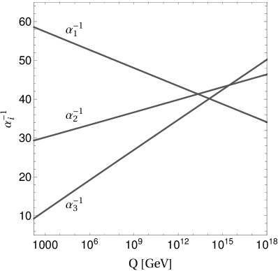
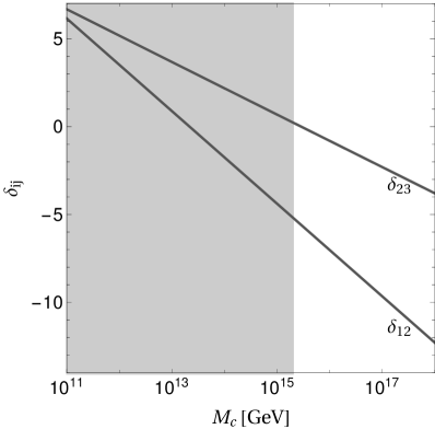
Figure 2: Left panel: Running of $\alpha_{i}^{-1}$ with respect to renormalization scale $Q$ for case A. Right panel: The values of $\delta_{23}$ and $\delta_{12}$ required by the conditions given in Eq. (15). The gray region is excluded by the current lower bound on the proton lifetime.

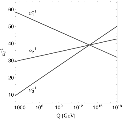
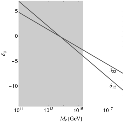
Figure 3: Same as in Fig. 2, but for the case B.

With light higgsinos (Fig. 3), one obtains a rather accurate gauge coupling unification without correction terms at $Q\sim 10^{14}~{}\text{GeV}$. As a consequence, the difference $|\delta_{23}-\delta_{12}|$ is smaller in case B than in case A. In the right panel of Fig. 2 and Fig. 3 the gray region ($M_{c}<10^{15}~{}\mathrm{GeV}$) is excluded by the current lower bound on the proton lifetime (see Section 3).

In higher-dimensional theories gauge couplings receive power-law quantum corrections for scales above the compactification scale, $\Lambda>M_{c}$. In six dimensions one has at one-loop order [33],

$$\delta\left(\frac{1}{g_{i}^{2}(\Lambda)}\right)=-\frac{b\pi}{16\pi^{2}}\left(\frac{\Lambda}{M_{c}}\right)^{2}\ ,$$ (16)

where $b$ is the one-loop coefficient of the $\beta$-function. For the gauge group $SO(10)$ with $\mathcal{N}=2$ supersymmetry, eight 10-plets and six 16-plets, which corresponds to the model in [28], one obtains $b=12$. Due to the large number of bulk matter fields one reaches the strong coupling regime, $1/g_{i}^{2}\approx 0$, already close to the compactification scale, at $\Lambda/M_{c}\simeq 3.7$. Assuming now gauge coupling unification at strong coupling at a cutoff $\Lambda>M_{c}$[40], one can estimate the size of brane kinetic terms due to quantum corrections,

$$G^{p}_{i}=\frac{b_{p,i}}{8\pi^{2}}\ln\left(\frac{\Lambda}{M_{c}}\right)\ .$$ (17)

Here $b_{p,i}$ is the one-loop $\beta$-function of a 4D coupling at fixed point $\zeta_{p}$, which describes the logarithmic running due to bulk zero-modes with nonvanishing wave function at $p$. This logarithmic contribution is relevant for the ‘differential running’, i.e., the difference between contributions to different brane kinetic terms [41, 8]. In general, contributions of higher Kaluza-Klein (KK) modes can also lead to power corrections in the differential running. However, in the considered model, such terms do not appear [38].

At the fixed point $\zeta_{\rm PS}$, with unbroken subgroup $SU(4)\times SU(2)_{\rm L}\times SU(2)_{\rm R}$, the bulk fields yield the following chiral superfields with positive parity [28]: $\psi,\chi,\Psi:(4^{*},1,2)$; $\psi^{c},\chi^{c},\Psi^{c}:(4,1,2)$; $H_{1},H_{2}:(1,2,2)$; $H_{3},\ldots H_{8}:(6,1,1)$, and the $\mathcal{N}=1$ vector multiplets contained in $45:(15,1,1)+(1,3,1)+(1,1,3)$. The three brane kinetic terms are given by

$$G^{\rm PS}_{1}=\frac{b_{4}}{8\pi^{2}}\ln\left(\frac{\Lambda}{M_{c}}\right)\ ,\quad G^{\rm PS}_{2}=\frac{b_{2L}}{8\pi^{2}}\ln\left(\frac{\Lambda}{M_{c}}\right)\ ,\quad G^{\rm PS}_{3}=\frac{b_{2R}}{8\pi^{2}}\ln\left(\frac{\Lambda}{M_{c}}\right)\ .$$ (18)

Inserting the indices for the above representations [39] into the expression for the one-loop $\beta$-function, one finds $b_{4}=0$, $b_{2L}=-4$ and $b_{2R}=8$.

Analogously, at the fixed point $\zeta_{\rm fl}$, with unbroken subgroup $SU(5)^{\prime}\times U(1)^{\prime}$, the chiral superfields with positive parity are [28]: $\psi:5^{{}^{\prime}*}_{3}+1^{\prime}_{-5}$; $\chi,\Psi:10^{\prime}_{-1}$; $\psi^{c}:5^{\prime}_{-3},1^{\prime}_{5}$; $\chi^{c},\Psi^{c}:10^{*}_{1}$; $H_{1}\ldots H_{8}:4\times 5^{{}^{\prime}*}_{-2},4\times 5^{\prime}_{2}$. For the $\mathcal{N}=1$ vector multiplet one has $45:24^{\prime}_{0},1^{\prime}_{0}$. The two brane kinetic terms read

$$G^{\rm fl}_{1}=\frac{b_{5^{\prime}}}{8\pi^{2}}\ln\left(\frac{\Lambda}{M_{c}}\right)\ ,\quad G^{\rm fl}_{2}=\frac{b_{1^{\prime}}}{8\pi^{2}}\ln\left(\frac{\Lambda}{M_{c}}\right)\ .$$ (19)

Inserting the indices of the $SU(5)^{\prime}$ representations [39] into the one-loop $\beta$-function, one obtains $b_{5^{\prime}}=-4$ and $b_{1^{\prime}}=17/8$.

Eqs. (18) and (19), together with Eqs. (15) and $\Lambda/M_{c}\simeq 3.7$, yield the result

$$\delta_{23}=-0.8\ ,\quad\delta_{12}=3.1\ .$$ (20)

Inspection of Fig. 2 and Fig. 3 shows that this result is incompatible with the values of $\delta_{23}$ and $\delta_{12}$ required by gauge coupling unification. Hence, given just the bulk field content of the considered model, unification of gauge couplings cannot be achieved at strong coupling. However, the differential running beyond the compactification scale is strongly model dependent. Adding further heavy vector-like pairs of bulk fields and/or $\mathcal{N}=1$ split multiplets at the branes does not change the low-energy phenomenology, but it significantly modifies the values of $\delta_{23}$ and $\delta_{12}$. Indeed, orbifold compactifications of the heterotic string generically yield as many $\mathcal{N}=1$ split multiplets on the branes as bulk fields. Adding on the PS brane $N_{4}$ pairs of $(4,2,1),(4^{*},2,1)$, $\bar{N}_{4}$ pairs of $(4,1,2),(4^{*},1,2)$, $N_{6}$ copies of $(6,1,1)$ and $N_{2}$ copies of $(1,2,2)$, and on the flipped brane $N_{5^{\prime}}$ pairs of $5^{\prime}_{2},5^{{}^{\prime}*}_{-2}$, $N_{5^{\prime},1^{\prime}}$ pairs of $5^{{}^{\prime}*}_{3},1^{\prime}_{-5},5^{\prime}_{-3},1^{\prime}_{5}$, and $N_{10^{\prime}}$ pairs of $10^{\prime}_{-1},10^{{}^{\prime}*}_{1}$, one obtains

$$\begin{split}\delta_{23}=&\frac{1}{2\pi}\left(-4+2N_{4}-2\bar{N}_{4}-N_{6}+N_{2}\right)\ln\left(\frac{\Lambda}{M_{c}}\right)\ ,\\ \delta_{12}=&\frac{1}{2\pi}\left(\frac{44}{5}-\frac{2}{5}\left(2N_{4}-2\bar{N}_{4}-N_{6}+N_{2}\right)\right.\\ &\left.\qquad+\frac{3}{25}\left(49-23N_{10^{\prime}}-6N_{5^{\prime}}-N_{5^{\prime},1^{\prime}}\right)\right)\ln\left(\frac{\Lambda}{M_{c}}\right)\ .\end{split}$$ (21)

As an example, the choice $N_{4}=N_{2}=4$, $\bar{N}_{4}=N_{5^{\prime}}=N_{5^{\prime},1^{\prime}}=3$, $N_{6}=1$, $N_{10^{\prime}}=12$, with $\Lambda/M_{c}\simeq 3.7$, yields $\delta_{23}=0.2$, $\delta_{12}=-5.3$, in agreement with gauge coupling unification for case A, the THDM without light higgsinos. One can also find examples that give gauge coupling unification in case B. However, we do not want to emphasize this possibility since the considered model is incomplete in any case. For the bulk field content of our model the irreducible $SO(10)$ 6D anomalies are satisfied. But one also has to satisfy irreducible and reducible gravitational and $U(1)_{A}$ anomalies as well as fixed point anomalies [42, 43], which requires further bulk and brane fields. Hence, in the considered model, we cannot compute the compactification scale, we can only demonstrate that phenomenologically acceptable extensions of the model can be consistent with gauge coupling unification and proton decay.

The required brane kinetic terms are rather large, corresponding to corrections of $\alpha_{i}^{-1}$ up to 10%. Because of the large number of bulk and brane fields the perturbative treatment of the model breaks down close to the compactification scale $M_{c}\simeq 2\times 10^{15}~{}\mathrm{GeV}$. We conclude that starting from the considered model, the compactification scale cannot be consistently increased much by adding further vector-like fields. Hence, our model is only consistent for a proton lifetime close to the current lower bound.

3 Proton decay

For the considered 6D $SO(10)$ model proton decay rates can be evaluated in the standard manner. The model determines the currents that couple to vector bosons carrying $B-L$ charge. Knowing the zero-mode wave functions of quarks and leptons, their couplings to the various vector boson KK-modes can be computed. Integrating out the vector boson KK-modes provides the dimension-six operators whose matrix elements determine the proton decay rates. As we shall see, a special feature of our model is the flavour structure of these operators, which leads to unexpected branching fractions.

3.1 Effective operators and decay widths

The interaction Lagrangian of the 16-plets with $SO(10)$ gauge fields is given by

$$\mathcal{L}_{I}=\int d^{4}\theta\,\left(\overline{\psi}\,e^{2g_{\rm 6D}V}\,\psi+\overline{\psi^{c}}\,e^{-2g_{\rm 6D}V}\,\psi^{c}+\overline{\chi}\,e^{2g_{\rm 6D}V}\,\chi+\overline{\chi^{c}}\,e^{-2g_{\rm 6D}V}\,\chi^{c}\right)\ ,$$ (22)

where $V$ is a vector field in the adjoint representation of $SO(10)$. The decomposition of the 45-plet with respect to $SU(3)_{C}\times SU(2)_{L}\times U(1)_{Y}\times U(1)_{X}$ is listed in Table 1.

$SU(5)\times U(1)_{X}$	$SU(3)_{C}\times SU(2)_{L}\times U(1)_{Y}\times U(1)_{X}$	$U(1)_{B-L}$
$(24,0)$	$(8,1,0,0)$	0
	$(3,2,-\frac{5}{6},0)+(\overline{3},2,\frac{5}{6},0)$	$\mp\frac{2}{3}$
	$(1,3,0,0)$	0
	$(1,1,0,0)$	0
$(10,4)+(\overline{10},-4)$	$(3,2,\frac{1}{6},4)+(\overline{3},2,-\frac{1}{6},-4)$	$\mp\frac{2}{3}$
	$(\overline{3},1,-\frac{2}{3},4)+(3,1,\frac{2}{3},-4)$	$\mp\frac{4}{3}$
	$(1,1,1,4)+(1,1,-1,-4)$	0
$(1,0)$	$(1,1,0,0)$	0

Table 1: The decomposition of ${\bf 45}$-plet of $SO(10)$.

Proton decay is induced by the exchange of the gauge bosons $X\sim(3,2,-\frac{5}{6})$, $Y\sim(3,2,\frac{1}{6})$ and $Z\sim(\overline{3},1,-\frac{2}{3})$, which carry nonzero $B-L$ charge. The terms in Eq. (22), involving these gauge bosons and massless fermions, are described by the 4D effective Lagrangian

$${\cal L}_{\rm 4D}=-i\frac{g_{\rm 4D}}{\sqrt{2}}\sum_{m,n\geq 0} \left[\overline{X}_{a\mu}^{(2m,2n+1)}{\cal X}^{\mu}_{a}(m,n)+\overline{Y}_{a\mu}^{(2m+1,2n+1)}{\cal Y}^{\mu}_{a}(m,n)\right.$$

$$+\left.\overline{Z}_{a\mu}^{(2m+1,2n)}{\cal Z}^{\mu}_{a}(m,n)\right]+{\rm h.c.}\,,$$ (23)

where $g_{\rm 4D}=g_{\rm 6D}/\sqrt{V_{2}}$ is the 4D gauge coupling. The three currents relevant for proton decay are given by

$${\cal X}^{\mu}_{a}(m,n)=\sum_{\alpha i}\,\big{[} I^{(1)}_{i\alpha}(m,n)\,\epsilon_{abc}\,\overline{q}_{bi}\,\gamma^{\mu}\,u^{c}_{c\alpha}+I^{(1)*}_{i\alpha}(m,n)\,\overline{e^{c}}_{\alpha}\,\gamma^{\mu}\,q_{ai}$$

$$- I^{(2)}_{i\alpha}(m,n)\,\overline{d^{c}}_{a\alpha}\,\gamma^{\mu}\,l_{i}\big{]}\,,$$ (24)

$${\cal Y}^{\mu}_{a}(m,n)=\sum_{\alpha,i}\,\big{[} I^{(3)}_{i\alpha}(m,n)\,\epsilon_{abc}\,\overline{q}_{bi}\,\gamma^{\mu}\,d^{c}_{c\alpha}+I^{(3)*}_{i\alpha}(m,n)\,\overline{n^{c}}_{\alpha}\,\gamma^{\mu}\,q_{ai}\,$$

$$- I^{(4)}_{i\alpha}(m,n)\,\overline{u^{c}}_{a\alpha}\,\gamma^{\mu}\,l_{i}\big{]}\,,$$ (25)

$${\cal Z}^{\mu}_{a}(m,n)=\sum_{\alpha,\beta}\,\big{[} I^{(5)}_{\alpha\beta}(m,n)\,\overline{e^{c}}_{\alpha}\,\gamma^{\mu}\,d^{c}_{a\beta}\,+I^{(5)*}_{\alpha\beta}(m,n)\,\overline{n^{c}}_{\beta}\,\gamma^{\mu}\,u^{c}_{a\alpha}\,\big{]}$$

$$-\sum_{i,j}\, I^{(6)}_{ij}(m,n)\,\overline{q}_{ai}\,\gamma^{\mu}\,l_{j}\,.$$ (26)

Here $a,b,c=1,2,3$ are color indices, $i,j=1,2,3$ and $\alpha,\beta=1,...,4$ are flavour indices. $m,n=0,1,2,...$ label the KK-modes of the $X$-, $Y$- and $Z$-bosons. The dimensionless coefficients $I^{(r)}(m,n)$ ($r=1,...,6$) arise from overlaps between the profiles of KK-modes of gauge bosons and zero-modes of fermions. Their explicit expressions are given in Appendix A.

We observe that the currents coupled to the KK-modes of the $X$-, $Y$- and $Z$-bosons do not conserve flavour, i.e., one has $I_{i\alpha}^{(r)}(m,n)\neq 0$ for $i\neq\alpha$ in Eqs. (24), (25) and (26). This is in contrast to 4D GUTs where the couplings to $X$, $Y$ and $Z$ are flavour diagonal [14, 13]. The origin of this effect can be attributed to the fact that the three flavours of the SM quarks and leptons arise from the zero-modes of two bulk 16-plets in our model. As we will show at the end of this section, this flavour non-diagonal current, together with flavour non-diagonal mass matrices, gives rise to a proton decay pattern which is qualitatively different from that predicted in the 4D GUT models.

After integrating out the KK tower of $X$-, $Y$- and $Z$-bosons, one obtains from Eq. (3.1) the following effective operators for the proton decay:

$$-{\cal L}^{\rm eff}_{\rm 4D}=\frac{g_{\rm 4D}^{2}}{2} \sum_{\alpha,\beta}\,\sum_{i,j}\,\epsilon_{abc}\big{[}C^{(1)}_{i\alpha j\beta}\,\overline{u^{c}}_{c\beta}\gamma^{\mu}q_{bj}\,\,\overline{e^{c}}_{\alpha}\gamma_{\mu}q_{ai}-C^{(2)}_{i\alpha j\beta}\,\,\overline{u^{c}}_{c\beta}\gamma^{\mu}q_{bj}\,\,\overline{d^{c}}_{a\alpha}\gamma_{\mu}l_{i}$$

$$+C^{(3)}_{i\alpha j\beta}\,\,\overline{d^{c}}_{c\beta}\gamma^{\mu}q_{bj}\,\,\overline{n^{c}}_{\alpha}\gamma_{\mu}q_{ai}-C^{(4)}_{i\alpha j\beta}\,\,\overline{d^{c}}_{c\beta}\gamma^{\mu}q_{bj}\,\,\overline{u^{c}}_{a\alpha}\gamma_{\mu}l_{i}\big{]}+{\rm h.c.\,,}$$ (27)

with the coefficients

$$\begin{split}C^{(1)}_{i\alpha j\beta}&=\sum_{m,n}\frac{1}{M_{X}^{2}(m,n)}\,I^{(1)*}_{j\beta}(m,n)\,I^{(1)*}_{i\alpha}(m,n)\,,\\ C^{(2)}_{i\alpha j\beta}&=\sum_{m,n}\frac{1}{M_{X}^{2}(m,n)}\,I^{(1)*}_{j\beta}(m,n)\,I^{(2)}_{i\alpha}(m,n)\,,\\ C^{(3)}_{i\alpha j\beta}&=\sum_{m,n}\frac{1}{M_{Y}^{2}(m,n)}\,I^{(3)*}_{j\beta}(m,n)\,I^{(3)*}_{i\alpha}(m,n)\,,\\ C^{(4)}_{i\alpha j\beta}&=\sum_{m,n}\frac{1}{M_{Y}^{2}(m,n)}\,I^{(3)*}_{j\beta}(m,n)\,I^{(4)}_{i\alpha}(m,n)\,,\end{split}$$ (28)

where the vector boson masses are given by

$$\begin{split}M_{X}^{2}(m,n)&=4\pi^{2}\left(\frac{(2m)^{2}}{R_{1}^{2}}+\frac{(2n+1)^{2}}{R_{2}^{2}}\right)\,,\\ M_{Y}^{2}(m,n)&=4\pi^{2}\left(\frac{(2m+1)^{2}}{R_{1}^{2}}+\frac{(2n+1)^{2}}{R_{2}^{2}}\right)\,.\end{split}$$ (29)

The $Z$-bosons by themselves do not lead to dimension-six operators that induce proton decay. Their contribution only arises after electroweak symmetry breaking through their mixing with some $Y$-bosons. We do not include these contributions in the list of operators given in Eq. (3.1). Moreover, the third term in Eq. (3.1) is irrelevant for proton decay as it involves heavy singlet neutrinos. Using Fierz reordering, the remaining terms can be rewritten as

$$\begin{split}{\cal L}^{\rm eff}_{\rm 4D}=g_{\rm 4D}^{2}\sum_{\alpha,\beta}\,\sum_{i,j}\,&\big{[}C^{(11)}_{i\alpha j\beta}\,\epsilon_{abc}\,\overline{e^{c}}_{\alpha}\overline{u^{c}}_{a\beta}u_{bj}d_{ci}\,\\ &+C^{(24)}_{i\alpha j\beta}\,\epsilon_{abc}\,\overline{d^{c}}_{a\alpha}\overline{u^{c}}_{b\beta}\left(d_{cj}\nu_{i}\,-\,u_{cj}e_{i}\right)\big{]}+{\rm h.c.\,,}\end{split}$$ (30)

with

$$\begin{split}C^{(11)}_{i\alpha j\beta}&=C^{(1)}_{i\alpha j\beta}+C^{(1)}_{j\alpha i\beta}\,,\\ C^{(24)}_{i\alpha j\beta}&=C^{(2)}_{i\alpha j\beta}-C^{(4)}_{i\beta j\alpha}\,.\end{split}$$ (31)

The operators in the physical basis are obtained using the unitary transformations between weak ($f$) and mass ($f^{\prime}$) eigenstates,

$$f=U_{f}\,f^{\prime}\,,$$ (32)

where $f=u,d,e,\nu,u^{c},d^{c},e^{c}$. In the present framework, the unitary matrices $U_{u^{c}}$, $U_{d^{c}}$ and $U_{e^{c}}$ are of dimension $4\times 4$, while $U_{u}$, $U_{d}$, $U_{e}$ and $U_{\nu}$ are $3\times 3$ matrices. Changing from weak to mass eigenstates, Eq. (30) becomes

$$\begin{split}{\cal L}^{\rm eff}_{\rm 4D}=g_{\rm 4D}^{2}\sum_{\gamma,\delta}\,\sum_{l,k}\,&\big{[}d^{(1)}_{l\gamma k\delta}\,\epsilon_{abc}\,\overline{e^{c}}^{\prime}_{\gamma}\overline{u^{c}}^{\prime}_{a\delta}u^{\prime}_{bk}d^{\prime}_{cl}\,\\ &+d^{(2)}_{l\gamma k\delta}\,\epsilon_{abc}\,\overline{d^{c}}^{\prime}_{a\gamma}\overline{u^{c}}^{\prime}_{b\delta}u^{\prime}_{ck}e^{\prime}_{l}+d^{(3)}_{l\gamma k\delta}\,\epsilon_{abc}\,\overline{d^{c}}^{\prime}_{a\gamma}\overline{u^{c}}^{\prime}_{b\delta}d^{\prime}_{ck}\nu^{\prime}_{l}\,\big{]}+{\rm h.c.\,,}\end{split}$$ (33)

where

$$\begin{split}d^{(1)}_{l\gamma k\delta}&=\sum_{\alpha,\beta}\,\sum_{i,j}\,C^{(11)}_{i\alpha j\beta}\,\left(U_{e^{c}}^{*}\right)_{\alpha\gamma}\,\left(U_{u^{c}}^{*}\right)_{\beta\delta}\,\left(U_{u}\right)_{jk}\,\left(U_{d}\right)_{il}\,,\\ d^{(2)}_{l\gamma k\delta}&=-\sum_{\alpha,\beta}\,\sum_{ij}\,C^{(24)}_{i\alpha j\beta}\,\left(U_{d^{c}}^{*}\right)_{\alpha\gamma}\,\left(U_{u^{c}}^{*}\right)_{\beta\delta}\,\left(U_{u}\right)_{jk}\,\left(U_{e}\right)_{il}\,,\\ d^{(3)}_{l\gamma k\delta}&=\sum_{\alpha,\beta}\,\sum_{ij}\,C^{(24)}_{i\alpha j\beta}\,\left(U_{d^{c}}^{*}\right)_{\alpha\gamma}\,\left(U_{u^{c}}^{*}\right)_{\beta\delta}\,\left(U_{d}\right)_{jk}\,\left(U_{\nu}\right)_{il}\,.\end{split}$$ (34)

Note that the matrix $U_{\nu}$ drops out in proton decay branching fractions since we sum over neutrino flavours in the final state.

The partial widths of the various proton decay channels can be evaluated based on Eq. (33). All operators conserve $B-L$, and therefore the proton decays into an anti-lepton and a meson. The relevant hadronic matrix elements between proton and meson states is obtained using chiral perturbation theory [44, 45]. The resulting partial decay widths read [46]:

$$\Gamma[p\to e_{i}^{+}\pi^{0}] =\frac{(m_{p}^{2}-m_{\pi^{0}}^{2})^{2}}{32\,\pi\,m_{p}^{3}f_{\pi}^{2}}\,\alpha^{2}A^{2}g_{\rm 4D}^{4}\left(\frac{1+D+F}{\sqrt{2}}\right)^{2}\left(\left|d^{(1)}_{1i11}\right|^{2}+\left|d^{(2)}_{i111}\right|^{2}\right),$$

$$\Gamma[p\to\overline{\nu}\pi^{+}] =\frac{(m_{p}^{2}-m_{\pi^{\pm}}^{2})^{2}}{32\,\pi\,m_{p}^{3}f_{\pi}^{2}}\,\alpha^{2}A^{2}g_{\rm 4D}^{4}\left(1+D+F\right)^{2}\sum_{i=1}^{3}\left|d^{(3)}_{i111}\right|^{2}\,,$$

$$\Gamma[p\to e_{i}^{+}K^{0}] =\frac{(m_{p}^{2}-m_{K^{0}}^{2})^{2}}{32\,\pi\,m_{p}^{3}f_{\pi}^{2}}\,\alpha^{2}A^{2}g_{\rm 4D}^{4}\left(1+(D-F)\frac{m_{p}}{m_{B}}\right)^{2}\left(\left|d^{(1)}_{2i11}\right|^{2}+\left|d^{(2)}_{i211}\right|^{2}\right),$$

$$\Gamma[p\to\overline{\nu}K^{+}] =\frac{(m_{p}^{2}-m_{K^{\pm}}^{2})^{2}}{32\,\pi\,m_{p}^{3}f_{\pi}^{2}}\,\alpha^{2}A^{2}g_{\rm 4D}^{4}\sum_{i=1}^{3}\left|\frac{2D}{3}\frac{m_{p}}{m_{B}}d^{(3)}_{i211}+\left(1+\frac{D+3F}{3}\frac{m_{p}}{m_{B}}\right)d^{(3)}_{i121}\right|^{2},$$

$$\Gamma[p\to e_{i}^{+}\eta] =\frac{(m_{p}^{2}-m_{\eta}^{2})^{2}}{32\,\pi\,m_{p}^{3}f_{\pi}^{2}}\,\alpha^{2}A^{2}g_{\rm 4D}^{4}\left(\frac{1+D-3F}{\sqrt{6}}\right)^{2}\left(\left|d^{(1)}_{1i11}\right|^{2}+\left|d^{(2)}_{i111}\right|^{2}\right).$$ (35)

Here $e_{i}^{+}=(e^{+},\mu^{+})$, $m_{h}$ ($h=p,\pi^{0},\pi^{\pm},K^{0},K^{\pm},\eta$) denotes the mass of hadron $h$, $f_{\pi}$ is the pion decay constant and $m_{B}$ is the average baryon mass. The factors $\alpha$, $D$ and $F$ are parameters of the chiral Lagrangian while $A$ incorporates renormalization group running effects of the hadronic matrix elements.

3.2 Numerical results

We now evaluate the partial proton decay widths for the two fits of the flavour spectrum performed in [28]. In the first one (Fit I), the Yukawa couplings and brane mass parameters of the model were determined by fitting fermion masses and mixing parameters using the $\chi^{2}$ minimization method. We obtained a very good fit with a minimum $\chi^{2}=0.5$; in this case, leptogenesis led to a baryon asymmetry two orders of magnitude below the observed value. We then performed another fit (Fit II) where the observed baryon asymmetry was used as a constraint, for which we obtained a minimum $\chi^{2}=0.95$. For both fits, we give the various unitary matrices $U_{f}$ that connect weak and mass eigenstates in Appendix B.

The effective couplings $C_{i}$ in Eq. (28) involve summations over the KK-modes of gauge bosons. We notice that the value of some of the $C_{i}$’s decrease slightly when contributions from higher KK-modes are taken into account because of destructive interference between different amplitudes. We also find that the values of these coefficients converge rapidly, and only the contributions from the first few KK-modes are relevant. We consider the first five modes, corresponding to $m,n=0,1,...,4$, for the evaluation of the partial widths.

We use the parameters $\alpha=0.01$ GeV³, $D=0.8$ and $F=0.46$ for the chiral Lagrangian parameters [46]. The parameter $A$ can be written as $A=A_{\rm SD}A_{\rm LD}$, where $A_{\rm LD}$ takes into account the renormalization effects from $M_{Z}$ to the proton mass scale while $A_{\rm SD}$ includes the short distance running effects from $M_{\rm GUT}$ to $M_{Z}$. For our calculation, we use $A_{\rm LD}=1.43$ and $A_{\rm SD}=2.26$ [47]. The values of hadron masses are taken from the PDG [16]. We use $m_{B}=1.15$ GeV as average baryon mass, the pion decay constant $f_{\pi}=130$ MeV, and we take $g_{\rm 4D}=0.57$. The compactification scale is identified with the mass of the lightest KK-mode of the $X$-, $Y$-bosons, which corresponds to $R_{1}=R_{2}=2\pi M_{c}^{-1}$.

The proton lifetime in a particular channel, $p\to\bar{l}+X$, is defined as

$$\tau/{\rm BR}[p\to\bar{l}+X]=1/\Gamma[p\to\bar{l}+X]\,,$$ (36)

where $\tau=1/\Gamma_{\rm total}$, and the branching ratio is ${\rm BR}[p\to\bar{l}+X]=\Gamma[p\to\bar{l}+X]/\Gamma_{\rm total}$. The current limits on the proton lifetime are at $90\%$ confidence level [36],

$$\tau/{\rm BR}[p\to e^{+}\pi^{0}]>1.6\times 10^{34}\,{\rm~{}yrs},\quad\tau/{\rm BR}[p\to\mu^{+}\pi^{0}]>7.7\times 10^{33}\,{\rm~{}yrs}\,.$$ (37)

With the aforementioned values of the various parameters, we obtain for Fit I,

$$\tau/{\rm BR}[p\to e^{+}\pi^{0}] = 1.6\times 10^{34}\,{\rm~{}yrs}\times\left(\frac{M_{c}}{2.2\times 10^{15}\,{\rm GeV}}\right)^{4}\,,$$

$$\tau/{\rm BR}[p\to\mu^{+}\pi^{0}] = 4.7\times 10^{34}\,{\rm~{}yrs}\times\left(\frac{M_{c}}{2.2\times 10^{15}\,{\rm GeV}}\right)^{4}\,,$$ (38)

and for Fit II,

$$\tau/{\rm BR}[p\to e^{+}\pi^{0}] = 1.6\times 10^{34}\,{\rm~{}yrs}\times\left(\frac{M_{c}}{2.0\times 10^{15}\,{\rm GeV}}\right)^{4}\,,$$

$$\tau/{\rm BR}[p\to\mu^{+}\pi^{0}] = 7.7\times 10^{33}\,{\rm~{}yrs}\times\left(\frac{M_{c}}{2.0\times 10^{15}\,{\rm GeV}}\right)^{4}\,,$$ (39)

In case of the latter, the channel $p\to\mu^{+}\pi^{0}$ provides an equally strong constraint as the positron channel. These numbers have to be compared with $\tau/{\rm BR}[p\to e^{+}\pi^{0}]\sim 2\times 10^{35}{\rm~{}yrs}$, the experimental reach of Hyper-Kamiokande [48], and with $\tau/{\rm BR}[p\to e^{+}\pi^{0}]\sim{\rm few}\times 10^{34}{\rm~{}yrs}$, the experimental reach of DUNE [49].

The various branching fractions obtained for Fit I and Fit II are displayed in Table 2.

Branching ratio [%]	Fit I	Fit II
${\rm BR}[p\to e^{+}\pi^{0}]$	46	23
${\rm BR}[p\to\mu^{+}\pi^{0}]$	17	51
${\rm BR}[p\to\bar{\nu}\pi^{+}]$	5	3
${\rm BR}[p\to e^{+}K^{0}]$	17	15
${\rm BR}[p\to\mu^{+}K^{0}]$	12	6
${\rm BR}[p\to\bar{\nu}K^{+}]$	1	1
${\rm BR}[p\to e^{+}\eta]$	$<$ 1	$<$ 1
${\rm BR}[p\to\mu^{+}\eta]$	$<$ 1	$<$ 1

Table 2: Proton decay branching fractions for two different fits to the flavour spectrum.

A noteworthy feature of these results is that the branching ratios of proton decay into the channels involving $e^{+}$ or $\mu^{+}$ are of the similar magnitude. The origin of this in the present model can be understood in the following way. First, as already mentioned earlier, the massless modes of quark and lepton generations have flavour non-diagonal overlaps with the KK-modes of heavy vector bosons. In particular, the flavours arising from the zero-modes of $\psi$ have comparable diagonal and non-diagonal couplings with the $X$- and $Y$-bosons. For example, zero-mode overlap integrals $I^{(1)}_{i\alpha}(0,0)$ ($I^{(2)}_{i\alpha}(0,0)$) of fermion zero-modes and vector bosons with $m=n=0$, that cause proton decay into a charged lepton with flavour $\alpha$ ($i$) and a quark with flavour $i$ ($\alpha$), are given by

$$\left(I^{(1)}_{i\alpha}(0,0)\right) = \left(\begin{array}[]{cccc}-0.12&-0.07&-1.0&0\\ 0.12&1.0&0.07&0\\ 0&0&0&0.45\\ \end{array}\right)\,,$$ (43)

$$\left(I^{(2)}_{i\alpha}(0,0)\right) = \left(\begin{array}[]{cccc}-0.28&-0.04(1+i)&0&0\\ 0.1(1-i)&1.0&0&0\\ 0&0&0.51&-0.51\\ \end{array}\right)\,,$$ (47)

These overlap integrals are properties of the wave functions of fermions and gauge bosons, which are unambiguously determined in the considered model and which do not depend on the Yukawa structure, i.e., on the particular fit of the flavour structure.

Second, as shown in Appendix B, some of the unitary matrices introduce large flavour mixings. In particular, the matrices $U_{u^{c}}$, $U_{d^{c}}$ and $U_{e^{c}}$ give rise to a strong mixing between the first and second generation of $u^{c}$, $d^{c}$ and $e^{c}$, respectively, both in Fit I and in Fit II. This feature depends on the Yukawa structure of the theory and hence the precise results are fit dependent. In the present framework, the non-diagonal gauge boson couplings as well as the flavour structure of the mass matrices give rise to an enhanced branching fraction ${\rm BR}[p\to\mu^{+}\pi^{0}]$, comparable to the branching fraction ${\rm BR}[p\to e^{+}\pi^{0}]$. This prediction is different from typical predictions made in the context of 4D GUTs, and it also distinguishes the 6D $SO(10)$ model with magnetic flux from the $SO(10)$ model without magnetic flux [22].

4 Summary and conclusions

In flux compactifications the quark-lepton generations are zero-modes with characteristic wave functions in the compact space. In the considered orbifold GUT model the Yukawa matrices are determined by the values of these wave functions at the orbifold fixed points, together with complex couplings of bulk fields at the fixed points which are generation independent. At each fixed point this leads to rank-one Yukawa matrices with $\mathcal{O}(1)$ entries. In addition there are large mass mixing terms with charge-conjugate split multiplets. The resulting up-quark, down-quark, charged lepton and Dirac neutrino mass matrices have large off-diagonal entries, and the same is true for the unitary matrices which diagonalize them. For two fits of the flavour spectrum, these matrices are given in Appendix B. A small mismatch of these matrices for up-quarks and down-quarks leads to small off-diagonal terms in the CKM matrix, whereas large off-diagonal terms appear in the PMNS matrix due to the seesaw mechanism.

As a consequence, the unitary matrices that connect weak and mass eigenstates lead to large flavour non-diagonal couplings of vector bosons with non-zero $B-L$ charge, whose exchange induces proton decay. This effect is enhanced by non-diagonal couplings of these heavy vector bosons to flavour eigenstates, which result from overlap integrals of vector boson and fermion mode functions. This is in contrast to 4D GUT models and other orbifold GUT models without flux, where the couplings of heavy vector bosons to flavour eigenstates are diagonal.

In the considered 6D $SO(10)$ orbifold GUT model gauge coupling unification can not be achieved at some cut-off scale beyond the compactification scale. Hence, the compactification scale cannot be computed. Gauge coupling unification requires the addition of further vector-like bulk and/or brane fields which would not affect the low-energy phenomenology. Due to the large number of vector-like fields the theory becomes strongly interacting already close to the compactification scale. It appears that matching the non-supersymmetric Standard Model to a higher-dimensional supersymmetric theory requires a compactification scale that is barely consistent with current constraints from proton decay. An unexpected prediction of our model is the similar size of the branching ratios $p\rightarrow e^{+}\pi^{0}$ and $p\rightarrow\mu^{+}\pi^{0}$ , where the latter one can even be dominant. This appears to be a generic feature of flux compactifications of higher-dimensional GUT models.

Appendix A Definition of overlap integrals

The dimensionless overlap integrals introduced in Section 3 are given as

$$\begin{split}I^{(1)}_{i^{\prime}\alpha^{\prime}}(m,n)&=\sqrt{V_{2}}\int d^{2}y\,\psi_{-+}^{(i^{\prime})*}(y)\,\psi_{++}^{(\alpha^{\prime})}(y)\,f_{X}^{(m,n)}(y)\,,\\ I^{(1)}_{34}(m,n)&=\sqrt{V_{2}}\int d^{2}y\,\chi_{--}^{(1)*}(y)\,\chi_{+-}^{(1)}(y)\,f_{X}^{(m,n)}(y)\,,\\ I^{(1)}_{i^{\prime}4}(m,n)&=I^{(1)}_{3\alpha^{\prime}}(m,n)=0\,.\end{split}$$ (48)

$$\begin{split}I^{(2)}_{i^{\prime}j^{\prime}}(m,n)&=\sqrt{V_{2}}\int d^{2}y\,\psi_{+-}^{(j^{\prime})*}(y)\,\psi_{--}^{(i^{\prime})}(y)\,f_{X}^{(m,n)}(y)\,,\\ I^{(2)}_{3(j^{\prime}+2)}(m,n)&=\sqrt{V_{2}}\int d^{2}y\,\chi_{++}^{(j^{\prime})*}(y)\,\chi_{-+}^{(1)}(y)\,f_{X}^{(m,n)}(y)\,,\\ I^{(2)}_{i^{\prime}(j^{\prime}+2)}(m,n)&=I^{(2)}_{3j^{\prime}}(m,n)=0\,.\end{split}$$ (49)

$$\begin{split}I^{(3)}_{i^{\prime}j^{\prime}}(m,n)&=\sqrt{V_{2}}\int d^{2}y\,\psi_{-+}^{(i^{\prime})*}(y)\,\psi_{+-}^{(j^{\prime})}(y)\,f_{Y}^{(m,n)}(y)\,,\\ I^{(3)}_{3(j^{\prime}+2)}(m,n)&=\sqrt{V_{2}}\int d^{2}y\,\chi_{--}^{(1)*}(y)\,\chi_{++}^{(j^{\prime})}(y)\,f_{Y}^{(m,n)}(y)\,,\\ I^{(3)}_{i^{\prime}(j^{\prime}+2)}(m,n)&=I^{(3)}_{3,j^{\prime}}(m,n)=0\,.\end{split}$$ (50)

$$\begin{split}I^{(4)}_{i^{\prime}\alpha^{\prime}}(m,n)&=\sqrt{V_{2}}\int d^{2}y\,\psi_{++}^{(\alpha^{\prime})*}(y)\,\psi_{--}^{(i^{\prime})}(y)\,f_{Y}^{(m,n)}(y)\,,\\ I^{(4)}_{34}(m,n)&=\sqrt{V_{2}}\int d^{2}y\,\chi_{+-}^{(1)*}(y)\,\chi_{-+}^{(1)}(y)\,f_{Y}^{(m,n)}(y)\,,\\ I^{(4)}_{i^{\prime}4}(m,n)&=I^{(4)}_{3\alpha^{\prime}}(m,n)=0\,.\end{split}$$ (51)

$$\begin{split}I^{(5)}_{\alpha^{\prime}i^{\prime}}(m,n)&=\sqrt{V_{2}}\int d^{2}y\,\psi_{++}^{(\alpha^{\prime})*}(y)\,\psi_{+-}^{(i^{\prime})}(y)\,f_{Z}^{(m,n)}(y)\,,\\ I^{(5)}_{4(j^{\prime}+2)}(m,n)&=\sqrt{V_{2}}\int d^{2}y\,\chi_{+-}^{(1)*}(y)\,\chi_{++}^{(j^{\prime})}(y)\,f_{Z}^{(m,n)}(y)\,,\\ I^{(5)}_{4j^{\prime}}(m,n)&=I^{(5)}_{44}(m,n)=0\,.\end{split}$$ (52)

$$\begin{split}I^{(6)}_{i^{\prime}j^{\prime}}(m,n)&=\sqrt{V_{2}}\int d^{2}y\,\psi_{-+}^{(i^{\prime})*}(y)\,\psi_{--}^{(j^{\prime})}(y)\,f_{Z}^{(m,n)}(y)\,,\\ I^{(6)}_{33}(m,n)&=\sqrt{V_{2}}\int d^{2}y\,\chi_{--}^{(1)*}(y)\,\chi_{-+}^{(1)}(y)\,f_{Z}^{(m,n)}(y)\,,\\ I^{(6)}_{i^{\prime}3}(m,n)&=I^{(6)}_{3j^{\prime}}(m,n)=0\,.\end{split}$$ (53)

Here $i^{\prime},j^{\prime}=1,2$ and $\alpha^{\prime}=1,2,3$ are the flavour indices introduced in the decomposition of the 16-plets in Section 2. The integration domain is given by $y_{1}\in[0,R_{1}/2]$ and $y_{2}\in[0,R_{2}]$. The volume of the orbifold is $V_{2}=R_{1}R_{2}/2$.

The mode functions of the gauge bosons are obtained from [22]. They read:

$$\begin{split}f_{X}^{(m,n)}(y)&=\sqrt{\frac{2}{V_{2}}}\,\cos\left[2\pi\left(2m\frac{y_{1}}{R_{1}}+(2n+1)\frac{y_{2}}{R_{2}}\right)\right]\,,\\ f_{Y}^{(m,n)}(y)&=\sqrt{\frac{2}{V_{2}}}\,\cos\left[2\pi\left((2m+1)\frac{y_{1}}{R_{1}}+(2n+1)\frac{y_{2}}{R_{2}}\right)\right]\,,\\ f_{Z}^{(m,n)}(y)&=\sqrt{\frac{2}{V_{2}}}\,\cos\left[2\pi\left((2m+1)\frac{y_{1}}{R_{1}}+2n\frac{y_{2}}{R_{2}}\right)\right]\,.\end{split}$$ (54)

The wavefunction profiles of quarks and leptons are obtained from the expression [27, 28]

$$\varphi_{\eta_{\rm PS},\eta_{\rm GG}}^{(j)}(y_{1},y_{2};N) = {\cal N}\exp\left(2\pi iN\tau\frac{y_{2}^{2}}{R_{2}^{2}}\right)\,\sum_{n\in{\mathbb{Z}}}\cos\left[2\pi\left(-2nN+j+\frac{k_{\rm PS}}{2}\right)\left(\frac{y_{1}}{R_{1}}+\tau\frac{y_{2}}{R_{2}}\right)\right]$$ (55)

$$\times \exp\left(2\pi i\tau N\left(n-\frac{j}{2N}\right)^{2}-i\pi\left(n-\frac{j}{2N}\right)(k_{\rm PS}\tau-k_{\rm GG})\right)$$

where $\eta_{\rm PS}=e^{i\pi k_{\rm PS}}$, $\eta_{\rm GG}=e^{i\pi k_{\rm GG}}$ and $k_{\rm PS},\,k_{\rm GG}=0,1$. Here $j=0,...,N$ for $k_{\rm PS}=k_{\rm GG}=0$ and $j=0,...,N-1$ otherwise. We identify

$$\psi^{(2)}_{\eta_{\rm PS},\eta_{\rm GG}}(y_{1},y_{2}) =\varphi^{(0)}_{\eta_{\rm PS},\eta_{\rm GG}}(y_{1},y_{2};2),~{}$$

$$\psi^{(1)}_{\eta_{\rm PS},\eta_{\rm GG}}(y_{1},y_{2}) =\varphi^{(1)}_{\eta_{\rm PS},\eta_{\rm GG}}(y_{1},y_{2};2),~{}$$

$$\psi^{(3)}_{++}(y_{1},y_{2}) =\varphi^{(2)}_{++}(y_{1},y_{2};2),~{}$$

$$\chi^{(1)}_{\eta_{\rm PS},\eta_{\rm GG}}(y_{1},y_{2}) =\varphi^{(0)}_{\eta_{\rm PS},\eta_{\rm GG}}(y_{1},y_{2};1),~{}$$

$$\chi^{(2)}_{++}(y_{1},y_{2}) =\varphi^{(1)}_{++}(y_{1},y_{2};1).$$ (56)

Appendix B Extraction of unitary matrices

The $3\times 3$ matrices $U_{f}$ for $f=u,d,e,\nu$ are obtained following the same procedure as in Appendix A of [28]. For $f=u^{c},d^{c},e^{c}$ the corresponding $4\times 4$ unitary matrices are obtained in the following way. Starting from the expressions for $M_{f}$ given in Eq. (A2) in [28], we obtain

$$H^{c}_{f}\equiv M_{f}^{\dagger}M_{f}=H^{c}_{f4}+H^{c}_{f3}\,,$$ (57)

where

$$\left(H^{c}_{f4}\right)_{\alpha\beta} = \mu^{f*}_{\alpha}\mu^{f}_{\beta}\,$$

$$\left(H^{c}_{f3}\right)_{\alpha\beta} = v_{f}^{2}\left(Y_{f}^{\dagger}Y_{f}\right)_{\alpha\beta}\,.$$ (58)

We determine $4\times 4$ unitary matrices $V_{4}^{f}$ such that

$$V_{4}^{f\dagger}H^{c}_{f4}V_{4}^{f}={\rm Diag.}\left(0,0,0,\tilde{\mu}_{f}^{2}\right)\equiv D_{4}^{f}\,,$$ (59)

where $\tilde{\mu}_{f}^{2}=\sum_{\alpha}|\mu_{\alpha}|^{2}$. We then obtain

$$\tilde{H}^{c}_{f}=V_{4}^{f\dagger}H^{c}_{f}V_{4}^{f}=D_{4}^{f}+V_{4}^{f\dagger}H^{c}_{f3}V_{4}^{f}\,,$$ (60)

and integrate out the heavy state to obtain an effective $3\times 3$ matrix for the light fermions, whose elements are

$$\left(\tilde{H}^{c}_{3f}\right)_{ij}=\left(\tilde{H}^{c}_{f}\right)_{ij}-\frac{1}{\tilde{\mu}_{f}^{2}}\left(\tilde{H}^{c}_{f}\right)_{i4}\left(\tilde{H}^{c}_{f}\right)_{j4}\,.$$ (61)

The matrix $\tilde{H}^{c}_{3f}$ is then diagonalized using a $3\times 3$ unitary matrix $V^{f}_{3}$ such that $V_{3}^{f\dagger}\tilde{H}^{c}_{3f}V_{3}^{f}=D_{3}^{f}$. Finally, the $4\times 4$ unitary matrix

$$U_{f}=V_{4}^{f}\left(\begin{array}[]{cc}V_{3}^{f}&0\\ 0&1\end{array}\right)$$ (62)

is constructed, which relates the weak eigenstates $(f)$ with mass eigenstates $(f^{\prime})$ such that $f=U_{f}f^{\prime}$, for $f=u^{c},d^{c},e^{c}$.

Following the above procedure, the unitary matrices obtained from Fit-I read

$$U_{u} = \left(\begin{array}[]{ccc}-0.9748+0.0693i&-0.2117+0.0008i&-0.0105\\ 0.2114\,-0.015i&-0.9761+0.0035i&-0.0486+0.0002i\\ 0&-0.0497&0.9988\\ \end{array}\right)\,,$$ (66)

$$U_{d} = \left(\begin{array}[]{ccc}-0.1438-0.9543i&-0.1447+0.2179i&-0.0156+0.0003i\\ -0.1905+0.1788i&-0.9611+0.013i&-0.0887+0.0047i\\ -0.0198&-0.088&0.9959\\ \end{array}\right)\,,$$ (70)

$$U_{e} = \left(\begin{array}[]{ccc}-0.0792-0.1946i&-0.7026+0.6796i&-0.0097-0.0152i\\ -0.9734+0.0162i&-0.0817-0.1944i&-0.0886+0.0008i\\ -0.0904&-0.0036&0.9959\\ \end{array}\right)\,,$$ (74)

$$U_{u^{c}} = \left(\begin{array}[]{cccc}0.1981\,+0.6784i&-0.4109+0.5744i&-0.0248+0.0347i&0\\ -0.1395-0.4804i&-0.2907+0.4053i&-0.0184+0.0245i&-0.7071\\ 0.1395\,+0.4804i&0.2909\,-0.4053i&0.0167\,-0.0245i&-0.7071\\ 0.0001&-0.0603&0.9982&-0.0012\\ \end{array}\right)\,,$$ (79)

$$U_{d^{c}} = \left(\begin{array}[]{cccc}-0.949-0.1635i&0.2576\,-0.0511i&0.0061\,+0.0604i&0\\ -0.0776+0.0864i&-0.2752+0.3064i&-0.443+0.4931i&0.\,+0.6144i\\ 0.0604\,-0.0672i&0.2143\,-0.2386i&0.3449\,-0.384i&0.\,+0.789i\\ -0.1725+0.1458i&-0.2797+0.7617i&0.204\,-0.4989i&0\\ \end{array}\right)\,,$$ (84)

$$U_{e^{c}} = \left(\begin{array}[]{cccc}0.7074&0.7053&-0.0473&0\\ -0.4998&0.4988&-0.0373&-0.7071\\ 0.4998&-0.4989&0.0355&-0.7071\\ -0.003&0.0698&0.9976&-0.0012\\ \end{array}\right)\,.$$ (89)

Correspondingly, the unitary matrices obtained from the Fit II are given by

$$U_{u} = \left(\begin{array}[]{ccc}-0.5613-0.8003i&-0.0123+0.2106i&0.0001\,-0.0018i\\ 0.1219\,+0.1722i&-0.0527+0.976i&0.0004\,-0.0082i\\ 0&0.0084&1.\\ \end{array}\right)\,,$$ (93)

$$U_{d} = \left(\begin{array}[]{ccc}-0.0205-0.9329i&-0.3053-0.1897i&-0.0116+0.0013i\\ 0.2196\,+0.2847i&-0.9294+0.0744i&-0.0379+0.0002i\\ 0.0092&-0.0385&0.9992\\ \end{array}\right)\,,$$ (97)

$$U_{e} = \left(\begin{array}[]{ccc}0.1388\,+0.1353i&-0.0003-0.0314i&-0.6933+0.6933i\\ 0.9743\,+0.0005i&-0.1128+0.0044i&0.\,-0.195i\\ 0.1149&0.9931&0.0225\\ \end{array}\right)\,,$$ (101)

$$U_{u^{c}} = \left(\begin{array}[]{cccc}0.504\,+0.4965i&-0.4195-0.1861i&0.4911\,+0.2182i&0\\ -0.3553-0.3509i&-0.8338-0.1323i&-0.1115+0.1543i&0.0417\\ 0.3563\,+0.3509i&-0.2391+0.1323i&-0.8061-0.1543i&0.0417\\ 0&0.0448&0.0383&0.9983\\ \end{array}\right)\,,$$ (106)

$$U_{d^{c}} = \left(\begin{array}[]{cccc}-0.4785-0.848i&0.1196\,+0.1932i&-0.0183+0.0012i&0\\ 0.0059\,+0.0097i&0.0296\,+0.0343i&-0.0553-0.0653i&0.\,+0.9952i\\ -0.0604-0.0995i&-0.3021-0.3501i&0.5647\,+0.6665i&0.\,+0.0975i\\ 0.1957&0.8558&0.4788&0\\ \end{array}\right)\,,$$ (111)

$$U_{e^{c}} = \left(\begin{array}[]{cccc}0.6851&-0.4879&0.5409&0\\ -0.5398&-0.8377&-0.072&0.0417\\ 0.4892&-0.2412&-0.8371&0.0417\\ 0.0021&0.045&0.0379&0.9983\\ \end{array}\right)\,.$$ (116)

References

• [1] J. C. Pati and A. Salam, “Unified Lepton-Hadron Symmetry and a Gauge Theory of the Basic Interactions,” Phys. Rev. D 8 (1973) 1240.
• [2] H. Georgi and S. L. Glashow, “Unity of All Elementary Particle Forces,” Phys. Rev. Lett.  32 (1974) 438.
• [3] S. Weinberg, “Supersymmetry at Ordinary Energies. 1. Masses and Conservation Laws,” Phys. Rev. D 26 (1982) 287.
• [4] N. Sakai and T. Yanagida, “Proton Decay in a Class of Supersymmetric Grand Unified Models,” Nucl. Phys. B 197 (1982) 533.
• [5] J. Hisano, H. Murayama and T. Yanagida, “Nucleon decay in the minimal supersymmetric SU(5) grand unification,” Nucl. Phys. B 402 (1993) 46 [hep-ph/9207279].
• [6] G. Altarelli and F. Feruglio, “SU(5) grand unification in extra dimensions and proton decay,” Phys. Lett. B 511 (2001) 257 [hep-ph/0102301].
• [7] L. J. Hall and Y. Nomura, “Gauge unification in higher dimensions,” Phys. Rev. D 64 (2001) 055003 [hep-ph/0103125].
• [8] A. Hebecker and J. March-Russell, “A Minimal S**1 / (Z(2) x Z-prime (2)) orbifold GUT,” Nucl. Phys. B 613 (2001) 3 [hep-ph/0106166].
• [9] H. Georgi, “The State of the Art—Gauge Theories,” AIP Conf. Proc.  23 (1975) 575.
• [10] H. Fritzsch and P. Minkowski, “Unified Interactions of Leptons and Hadrons,” Annals Phys.  93 (1975) 193.
• [11] S. M. Barr, “A New Symmetry Breaking Pattern for SO(10) and Proton Decay,” Phys. Lett.  112B (1982) 219.
• [12] J. P. Derendinger, J. E. Kim and D. V. Nanopoulos, “Anti-SU(5),” Phys. Lett.  139B (1984) 170.
• [13] P. Langacker, “Grand Unified Theories and Proton Decay,” Phys. Rept.  72, 185 (1981).
• [14] P. Nath and P. Fileviez Perez, “Proton stability in grand unified theories, in strings and in branes,” Phys. Rept.  441 (2007) 191 [hep-ph/0601023].
• [15] S. Raby, “Supersymmetric Grand Unified Theories : From Quarks to Strings via SUSY GUTs,” Lect. Notes Phys.  939 (2017) 1.
• [16] M. Tanabashi et al. [Particle Data Group], “Review of Particle Physics,” Phys. Rev. D 98 (2018) no.3, 030001.
• [17] R. Dermisek and A. Mafi, “SO(10) grand unification in five-dimensions: Proton decay and the mu problem,” Phys. Rev. D 65 (2002) 055002 [hep-ph/0108139].
• [18] A. Hebecker and J. March-Russell, “Proton decay signatures of orbifold GUTs,” Phys. Lett. B 539 (2002) 119 [hep-ph/0204037].
• [19] Q. Shafi and Z. Tavartkiladze, “Neutrino democracy, fermion mass hierarchies and proton decay from 5-D SU(5),” Phys. Rev. D 67 (2003) 075007 [hep-ph/0210181].
• [20] H. D. Kim and S. Raby, “Unification in 5D SO(10),” JHEP 0301 (2003) 056 [hep-ph/0212348].
• [21] M. L. Alciati, F. Feruglio, Y. Lin and A. Varagnolo, “Proton lifetime from SU(5) unification in extra dimensions,” JHEP 0503 (2005) 054 [hep-ph/0501086].
• [22] W. Buchmuller, L. Covi, D. Emmanuel-Costa and S. Wiesenfeldt, “Flavour structure and proton decay in 6D orbifold GUTs,” JHEP 0409 (2004) 004 [hep-ph/0407070].
• [23] F. J. de Anda and S. F. King, “$SU(3)\times SO(10)$ in 6d,” JHEP 1810 (2018) 128 [arXiv:1807.07078 [hep-ph]].
• [24] F. J. de Anda and S. F. King, “An $S_{4}\times SU(5)$ SUSY GUT of flavour in 6d,” JHEP 1807 (2018) 057 [arXiv:1803.04978 [hep-ph]].
• [25] W. Buchmuller, M. Dierigl, F. Ruehle and J. Schweizer, “Split symmetries,” Phys. Lett. B 750 (2015) 615 [arXiv:1507.06819 [hep-th]].
• [26] C. Bachas, “A Way to break supersymmetry,” hep-th/9503030.
• [27] W. Buchmuller and J. Schweizer, “Flavor mixings in flux compactifications,” Phys. Rev. D 95 (2017) no.7, 075024 [arXiv:1701.06935 [hep-ph]].
• [28] W. Buchmuller and K. M. Patel, “Flavor physics without flavor symmetries,” Phys. Rev. D 97 (2018) no.7, 075019 [arXiv:1712.06862 [hep-ph]].
• [29] G. Lee and C. E. M. Wagner, “Higgs bosons in heavy supersymmetry with an intermediate mA,” Phys. Rev. D 92 (2015) no.7, 075032 [arXiv:1508.00576 [hep-ph]].
• [30] E. Bagnaschi, F. Brümmer, W. Buchmüller, A. Voigt and G. Weiglein, “Vacuum stability and supersymmetry at high scales with two Higgs doublets,” JHEP 1603 (2016) 158 [arXiv:1512.07761 [hep-ph]].
• [31] V. S. Mummidi, V. P. K. and K. M. Patel, “Effects of heavy neutrinos on vacuum stability in two-Higgs-doublet model with GUT scale supersymmetry,” JHEP 1808 (2018) 134 [arXiv:1805.08005 [hep-ph]].
• [32] V. S. Mummidi and K. M. Patel, “Pseudo-Dirac Higgsino dark matter in GUT scale supersymmetry,” JHEP 1901 (2019) 224 [arXiv:1811.06297 [hep-ph]].
• [33] K. R. Dienes, E. Dudas and T. Gherghetta, “Grand unification at intermediate mass scales through extra dimensions,” Nucl. Phys. B 537 (1999) 47 [hep-ph/9806292].
• [34] S. Pokorski, K. Rolbiecki, G. G. Ross and K. Sakurai, “A new approach to gauge coupling unification and proton decay,” arXiv:1902.06093 [hep-ph].
• [35] J. R. Ellis, D. V. Nanopoulos and J. Walker, “Flipping SU(5) out of trouble,” Phys. Lett. B 550 (2002) 99 [hep-ph/0205336].
• [36] K. Abe et al. [Super-Kamiokande Collaboration], “Search for proton decay via $p\to e^{+}\pi^{0}$ and $p\to\mu^{+}\pi^{0}$ in 0.31  megaton·years exposure of the Super-Kamiokande water Cherenkov detector,” Phys. Rev. D 95 (2017) no.1, 012004 [arXiv:1610.03597 [hep-ex]].
• [37] T. Asaka, W. Buchmuller and L. Covi, “Gauge unification in six-dimensions,” Phys. Lett. B 523 (2001) 199 [hep-ph/0108021].
• [38] L. J. Hall, Y. Nomura, T. Okui and D. Tucker-Smith, “SO(10) unified theories in six-dimensions,” Phys. Rev. D 65 (2002) 035008 [hep-ph/0108071].
• [39] R. Slansky, “Group Theory for Unified Model Building,” Phys. Rept.  79 (1981) 1.
• [40] Y. Nomura, “Strongly coupled grand unification in higher dimensions,” Phys. Rev. D 65 (2002) 085036 [hep-ph/0108170].
• [41] Y. Nomura, D. Tucker-Smith and N. Weiner, “GUT breaking on the brane,” Nucl. Phys. B 613 (2001) 147 [hep-ph/0104041].
• [42] T. Asaka, W. Buchmuller and L. Covi, “Bulk and brane anomalies in six-dimensions,” Nucl. Phys. B 648 (2003) 231 [hep-ph/0209144].
• [43] G. von Gersdorff, N. Irges and M. Quiros, “Radiative brane mass terms in D greater than 5 orbifold gauge theories,” Phys. Lett. B 551 (2003) 351 [hep-ph/0210134].
• [44] M. Claudson, M. B. Wise and L. J. Hall, “Chiral Lagrangian for Deep Mine Physics,” Nucl. Phys. B 195, 297 (1982).
• [45] S. Chadha and M. Daniel, “Chiral Lagrangian Calculation of Nucleon Decay Modes Induced by $d=5$ Supersymmetric Operators,” Nucl. Phys. B 229, 105 (1983).
• [46] S. Aoki et al. [JLQCD Collaboration], “Nucleon decay matrix elements from lattice QCD,” Phys. Rev. D 62 (2000) 014506 [hep-lat/9911026].
• [47] R. Alonso, H. M. Chang, E. E. Jenkins, A. V. Manohar and B. Shotwell, “Renormalization group evolution of dimension-six baryon number violating operators,” Phys. Lett. B 734, 302 (2014) doi:10.1016/j.physletb.2014.05.065 [arXiv:1405.0486 [hep-ph]].
• [48] K. Abe et al. [Hyper-Kamiokande Collaboration], “Hyper-Kamiokande Design Report,” arXiv:1805.04163 [physics.ins-det].
• [49] R. Acciarri et al. [DUNE Collaboration], “Long-Baseline Neutrino Facility (LBNF) and Deep Underground Neutrino Experiment (DUNE) : Conceptual Design Report, Volume 2: The Physics Program for DUNE at LBNF,” arXiv:1512.06148 [physics.ins-det].