Operationally accessible bounds on fluctuations and entropy production in periodically driven systems
 

Abstract

For periodically driven systems, we derive a family of inequalities that relate entropy production with experimentally accessible data for the mean, its dependence on driving frequency, and the variance of a large class of observables. With one of these relations, overall entropy production can be bounded by just observing the time spent in a set of states. Among further consequences, the thermodynamic efficiency both of isothermal cyclic engines like molecular motors under a periodic load and of cyclic heat engines can be bounded using experimental data without requiring knowledge of the specific interactions within the system. We illustrate these results for a driven three-level system and for a colloidal Stirling engine.

Periodically driven open systems typically reach a periodic steady state since the coupling to the environment prevents unlimited heating up. For meso- and nanoscopic systems, such a steady state can still exhibit significant fluctuations Jung (1993). Beyond the quantum domain, in which such systems have found considerable attention recently, see, e.g., Gasparinetti et al. (2014); Shirai et al. (2016); Hartmann et al. (2017); Restrepo et al. (2018); Wang et al. (2018); Gambetta et al. (2019) and refs. therein, colloidal systems provide a major paradigm Ciliberto (2017). Likewise, chemical and biophysical systems on the molecular and cellular scale that are subjected to periodic mechanical, optical or chemical stimuli fall into this wide class, see, e.g., Hayashi et al. (2012); Erbas-Cakmak et al. (2015). Heat engines and cooling devices coupled cyclically to baths of different temperature provide a further paradigm Schmiedl and Seifert (2008); Esposito et al. (2010); Blickle and Bechinger (2012); Abah et al. (2012); Zhang et al. (2014); Verley et al. (2014); Campisi et al. (2015); Pekola (2015); Uzdin et al. (2015); Brandner et al. (2015); Roßnagel et al. (2016); Kosloff and Rezek (2017); Martinez et al. (2017),

One obvious question for any such system is whether or not the entropy production associated with the periodic driving can be inferred, or, at least, bounded, using only experimentally accessible observables without having detailed knowledge of the interactions or the internal structure of the system. This question is thus a non-trivial one whenever power input and power output are not both directly measurable, which is the case when not all degrees of freedom that couple to these currents are observable. This situation is inter alia typical for all systems undergoing chemical reactions. Likewise, it holds for systems driven by electric fields since one cannot observe the motion of all charges, in particular, in (soft) condensed matter systems.

For the arguably simpler class of non-equilibrium steady states in systems under constant, time-independent driving, a universal, experimentally accessible relation has recently been found that achieves this aim for classical systems. The so-called thermodynamic uncertainty relation (TUR) Barato and Seifert (2015); Gingrich et al. (2016)

$$\sigma D_{J}/J^{2}\geq 1$$ (1)

relates the entropy production rate $\sigma$ with the mean value of any current $J$ and its variance, or dispersion, $D_{J}$, all defined more precisely below. Besides stating a bound on the typically not directly accessible entropy production, this relation can also be interpreted as a bound on the precision of a process in the sense that small fluctuations, i.e., high precision or low uncertainty, requires a minimum amount of entropy production. As specific applications, the efficiency of molecular motors can be bounded using only experimental data Pietzonka et al. (2016a); Hwang and Hyeon (2018) and design principles for self-assembly can be derived Nguyen and Vaikuntanathan (2016). For steady-state heat engines, the relation shows that an inevitable side-effect of reaching Carnot efficiency at finite power are diverging power fluctuations Shiraishi et al. (2016); Campisi and Fazio (2016); Polettini and Esposito (2017); Pietzonka and Seifert (2018); Holubec and Ryabov (2018). Refinements and generalizations of the TUR have been found for diffusive dynamics Pietzonka et al. (2016b); Gingrich et al. (2017); Polettini et al. (2016), for data allocated over a finite time Pietzonka et al. (2017); Horowitz and Gingrich (2017); Dechant and ichi Sasa (2018); Pigolotti et al. (2017), for ballistic transport Brandner et al. (2018), for underdamped Langevin dynamics with and without magnetic fields Fischer et al. (2018); Dechant and Sasa (2018); Chun et al. (2019). Rather than looking at the fluctuations of currents, it is also possible to constrain the fluctuations of time-symmetric quantities like residence times or activity Nardini and Touchette (2018); Maes (2017); Terlizzi and Baiesi (2018) and the fluctuations of first passage times Gingrich and Horowitz (2017); Garrahan (2017). While a few quantum systems have been investigated, a systematic picture in the quantum realm is still missing Macieszczak et al. (2018); Agarwalla and Segal (2018); Carrega et al. (2019); Ptaszyński (2018); Guarnieri et al. (2019); Brandner et al. (2018).

An early counter-example has shown that a naive extension of the thermodynamic uncertainty relation from steady-state systems to periodically driven ones is not admissible Barato and Seifert (2016). Subsequent attempts to find an analog for periodically driven systems comprise Proesman and van den Broeck’s bound valid for time-symmetric driving that, however, for a small frequency of driving leads to a rather weak bound Proesmans and Van den Broeck (2017). Barato et al replace $\sigma$ in eq. (1) by a modified entropy production rate that requires detailed knowledge of dynamical properties of the whole system Barato et al. (2018a). In a follow up Barato et al. (2018b), a whole class of such modified entropy production rates were discussed that, from an operational perspective, are arguably not that useful since they require input that is typically not available in experiments. The same holds for our generalization introducing an effective entropy production for further types of currents Koyuk et al. (2019) and for a further scheme Rotskoff (2017). Recently, Proesmans and Horowitz introduced a modified uncertainty relation for hysteretic currents that overcomes some of the above mentioned short-comings Proesmans and Horowitz (2019). However, from the perspective of thermodynamic inference Seifert (2019), an operationally accessible relation, which allows to bound entropy production and which becomes the TUR for steady-state systems, is still missing for periodically driven systems.

As a main result of this Letter, for systems driven with a period $\mathcal{T}\equiv 2\pi/\Omega$, we will derive a family of universal bounds that relate, inter alia, the entropy production with fluctuations of observables. Applied to current fluctuations, we get specifically

$$\sigma(\Omega)D_{J}(\Omega)/J(\Omega)^{2}\geq[1-\Omega J^{\prime}(\Omega)/J(\Omega)]^{2}.$$ (2)

The left-hand side involves the same combination of variables as the ordinary TUR does, where we make the dependence on $\Omega$ explicit. The right-hand side additionally contains the derivative of the current with respect to the driving frequency, i.e., the response of the current to a slight change of the period of driving. In the special case of constant driving, this bound becomes the ordinary TUR, eq. (1), since then the current is formally independent of the driving frequency. Thus, the entropy production in a periodically driven system can be bounded using experimental data for the mean of any current, its fluctuations and its response to a slight change of driving frequency.

One consequence of this relation is that it provides a necessary condition for (almost) dissipation-less precision. The current must be proportional to the frequency of driving since then the right-hand side vanishes. This insight rationalizes the earlier construction of a dissipation-less Brownian clock Barato and Seifert (2016).

Applied to the efficiency $\eta\equiv P_{\mathrm{out}}/P_{\mathrm{in}}$ of isothermal cyclic engines that convert an input source of energy with mean $P_{\mathrm{in}}$ to an output power with mean $P_{\mathrm{out}}=P_{\mathrm{in}}-\sigma$, the relation implies

$$P_{\mathrm{out}}\leq\frac{1-\eta}{\eta}\frac{D_{{P_{\mathrm{out}}}}}{[1-\Omega P^{\prime}_{\mathrm{out}}(\Omega)/P_{\mathrm{out}}(\Omega)]^{2}}.$$ (3)

Hence, in general, the power of a cyclic engine vanishes at least linearly as its efficiency approaches the maximum value of 1. A finite power in this limit is, in principle, possible only if the current fluctuations diverge or if the output power is proportional to the cycling frequency of the engine. While the first option has been previously been derived for steady-state engines from the TUR Pietzonka et al. (2016a), the second one is genuine for periodically driven engines.

These results and the further ones derived and discussed below hold for systems described by a Markov dynamics on a set of states. The transition rate $k_{ij}(\tau)$ from state $i$ to state $j$ is time-periodic with $k_{ij}(\tau+\mathcal{T})=k_{ij}(\tau)$ and $0\leq\tau\leq\mathcal{T}$. In the long-time limit, the probability to find the system in state $i$ becomes periodic as well and will be denoted by $p^{\mathrm{ps}}_{i}(\tau;\Omega)$, where the corresponding driving frequency $\Omega$ is explicitly introduced through the second argument.

One class of fluctuating time-integrated current depends on the number of transitions between states

$$J_{T}^{d}\equiv\frac{1}{T}\int_{0}^{T}\mathrm{d}{t}\sum_{ij}\dot{n}_{ij}(t)d_{ij}(t)$$ (4)

with periodic increments $d_{ij}(t)=-d_{ji}(t)$ and $0\leq t\leq T$. Here, $n_{ij}(t)$ is the number of transitions from $i$ to $j$ up to time $t$ along a trajectory $i(t)$ of length $T$. In the long-time limit $T\to\infty$, the current in eq. (4) reaches the mean value

$$J^{d}(\Omega)\equiv\langle{J_{T}^{d}}\rangle=\frac{1}{\mathcal{T}}\int_{0}^{\mathcal{T}}\mathrm{d}{\tau}\sum_{i>j}j^{\mathrm{ps}}_{ij}(\tau;\Omega)d_{ij}(\tau),$$ (5)

where $j^{\mathrm{ps}}_{ij}(\tau;\Omega)\equiv p^{\mathrm{ps}}_{i}(\tau;\Omega)k_{ij}(\tau)-p^{\mathrm{ps}}_{j}(\tau;\Omega)k_{ji}(\tau)$. One example for the mean value of a current in eq. (4) is the entropy production

$$\sigma(\Omega)=\frac{1}{\mathcal{T}}\int_{0}^{\mathcal{T}}\mathrm{d}{\tau}\sum_{i>j}j^{\mathrm{ps}}_{ij}(\tau;\Omega)\ln\left(\frac{p^{\mathrm{ps}}_{i}(\tau;\Omega)k_{ij}(\tau)}{p^{\mathrm{ps}}_{j}(\tau;\Omega)k_{ji}(\tau)}\right).$$ (6)

A further class of current can be derived from the residence time in certain states as

$$J_{T}^{a}\equiv\frac{1}{T}\int_{0}^{T}\mathrm{d}{t}\sum_{i}\delta_{i(t),i}\dot{a}_{i}(t),$$ (7)

where $\delta_{i(t),i}$ is 1 if state $i$ is occupied at time $t$ and 0, otherwise. Here, the periodic increment can be written as a time-derivative of a state variable, e.g., for power input $\dot{a}_{i}(t)=\dot{E}_{i}(t)$, where $E_{i}(t)$ is the energy of state $i$. The mean value of eq. (7) is denoted by $J^{a}(\Omega)\equiv\langle{J_{T}^{a}}\rangle$. An arbitrary average current consists of a superposition of the two types of currents defined in eqs. (4) and (7), i.e., $J(\Omega)\equiv J^{d}(\Omega)+J^{a}(\Omega)$.

A second class of observables are called residence quantities that are defined as

$$A_{T}\equiv\frac{1}{T}\int_{0}^{T}\mathrm{d}{t}\sum_{i}\delta_{i(t),i}A_{i}(t)$$ (8)

with time-dependent periodic state variables $A_{i}(t)$ that cannot be written as time-derivatives. Simple examples of such a quantity are the average fraction of time $\tau_{k}$ spent in state $k$ during one cycle with increment $A_{i}(t)=\delta_{i,k}$ or the average energy with $A_{i}(t)=E_{i}(t)$. For long times, their mean value is given by

$$A(\Omega)\equiv\langle{A_{T}}\rangle=\frac{1}{\mathcal{T}}\int_{0}^{\mathcal{T}}\mathrm{d}{\tau}\sum_{i}p^{\mathrm{ps}}_{i}(\tau;\Omega)A_{i}(\tau).$$ (9)

Fluctuations of residence and current observables can be quantified via the diffusion coefficient

$$D_{X}(\Omega)\equiv\lim\limits_{T\to\infty}T\langle{\left(X_{T}-\langle{X_{T}}\rangle\right)^{2}}\rangle/2$$ (10)

with $X_{T}\in\{J^{d}_{T},J^{a}_{T},A_{T}\}$.

For the residence variable $A_{T}$ in eq. (8), we will show that the mean value $A(\Omega)$ and the fluctuations $D_{A}$ obey

$$\sigma(\Omega)D_{A}(\Omega)\geq[\Omega A^{\prime}(\Omega)]^{2}.$$ (11)

Thus, by measuring how the mean value of this observable changes with driving frequency, a lower bound on the entropy production can be obtained without knowing further details of the system. It is quite remarkable that by observing a variable that is even under time-reversal a bound on entropy production, which is a hallmark of broken time-reversal symmetry, can be inferred. There is no analog of this relation in the case of constant driving, since then the right-hand side vanishes.

As a first example, we illustrate relation (11) via an isothermal three state model with the following energy levels

$$E_{1}(t) =E^{c}_{1}\cos\Omega t+E^{s}_{1}\sin\Omega t+E_{1}^{0},$$

$$E_{2}(t) =E_{2}^{0},\quad\text{and}\quad E_{3}(t)=E_{3}^{0}.$$ (12)

The rates $k_{ij}(\tau)$

$$k_{ij}(t) =k^{0}_{ij}\exp\left[-\alpha(E_{i}(t)-E_{j}(t))\right],$$ (13)

$$k_{ji}(t) =k^{0}_{ij}\exp\left[(1-\alpha)(E_{i}(t)-E_{j}(t))\right]$$ (14)

fulfill the local detailed balance condition for any $\alpha$. Here, we have set $\beta=1$ and introduced a rate amplitude $k^{0}_{ij}$ for each link $(i,j)$.

We vary the driving frequency $\Omega$ for different energy amplitudes $E^{c}_{1}$ and fix all other parameters. The total entropy production can be estimated via eq. (11): the frequency-dependent fraction of residence time $\tau_{1}(\Omega)$ in state 1 and its diffusion coefficient $D_{\tau_{1}}(\Omega)$ are sufficient to obtain the estimator

$$\sigma_{\mathrm{est}}\equiv\left[\Omega\tau_{1}^{\prime}(\Omega)\right]^{2}/D_{\tau_{1}}(\Omega)\leq\sigma,$$ (15)

plotted in Fig. 1a as a function of the driving frequency $\Omega$ for different amplitudes $E^{c}_{1}$.

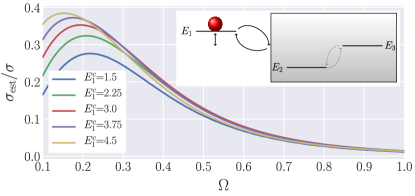
Figure 1: Ratio of estimator (15) and total entropy production (6) as a function of the driving frequency $\Omega$ for different energy amplitudes $E^{c}_{1}$ for the driven 3-state level (inset). The parameters $E^{s}_{1}=1.0,E_{1}^{0}=8.0,E_{2}^{0}=2.3,E_{3}^{0}=4.1,k^{0}_{12}=0.01,k^{0}_{23}=0.2,k^{0}_{13}=10.0,$ and $\alpha=0.1$ are kept fixed.

Hence, this simple estimate yields already up to 40% of the total entropy production.

The derivation of our main results (2) and (11) can be sketched as follows not . The diffusion coefficient $D_{G}(\Omega)$ for a quantity

$$G_{T}\equiv A_{T}+J^{a}_{T}+J^{d}_{T}$$ (16)

with mean $G(\Omega)\equiv\langle{G_{T}}\rangle$ can be bounded by

$$2D_{G}(\Omega)\geq(G(\Omega)-G(\Omega,\tilde{\Omega}))^{2}/[(\Omega/\tilde{\Omega}-1)^{2}\mathcal{S}(\Omega,\tilde{\Omega})],$$ (17)

where $\tilde{\Omega}$ is an arbitrary frequency and

$$\mathcal{S}(\Omega,\tilde{\Omega}) \equiv\frac{1}{\mathcal{T}}\int_{0}^{\mathcal{T}}\mathrm{d}{\tau}\sum_{i>j}\left[j^{\mathrm{ps}}_{ij}(\Omega\tau/\tilde{\Omega};\tilde{\Omega})\right]^{2}/t^{\mathrm{ps}}_{ij}(\tau;\Omega),$$ (18)

$$G(\Omega,\tilde{\Omega}) \equiv A(\tilde{\Omega})+(\Omega/\tilde{\Omega})J(\tilde{\Omega})$$ (19)

with $J(\tilde{\Omega})\equiv J^{a}(\tilde{\Omega})+J^{d}(\tilde{\Omega})$. Here, we introduced the probability current at frequency $\tilde{\Omega}$

$$j^{\mathrm{ps}}_{ij}(\Omega\tau/\tilde{\Omega};\tilde{\Omega})\equiv p^{\mathrm{ps}}_{i}(\Omega\tau/\tilde{\Omega};\tilde{\Omega})k_{ij}(\tau)-p^{\mathrm{ps}}_{j}(\Omega\tau/\tilde{\Omega};\tilde{\Omega})k_{ji}(\tau)$$ (20)

and the activity at link $(i,j)$

$$t^{\mathrm{ps}}_{ij}(\tau;\Omega)\equiv p^{\mathrm{ps}}_{i}(\tau;\Omega)k_{ij}(\tau)+p^{\mathrm{ps}}_{j}(\tau;\Omega)k_{ji}(\tau)$$ (21)

at the original frequency $\Omega$.

We choose either the increments $d_{ij}=\dot{a}_{i}=0$ or $A_{i}=0$ such that $G(\Omega)=J(\Omega)$ for currents and $G(\Omega)=A(\Omega)$ for residence quantities and take the limit $\tilde{\Omega}\to\Omega$. This leads to the following two inequalities

$$D_{J}(\Omega)C(\Omega)/J(\Omega)^{2} \geq(1-\Omega J^{\prime}(\Omega)/J(\Omega))^{2},$$ (22)

$$D_{A}(\Omega)C(\Omega)/A(\Omega)^{2} \geq(\Omega A^{\prime}(\Omega)/A(\Omega))^{2}.$$ (23)

Here, $C(\Omega)\in\{{2\mathcal{S}(\Omega),2\mathcal{A}(\Omega),\sigma(\Omega)}\}$ can be chosen as one of three cost terms with $\mathcal{S}(\Omega)\equiv\mathcal{S}(\Omega,\tilde{\Omega}=\Omega)$ and $\mathcal{A}(\Omega)\equiv 1/\mathcal{T}\int_{0}^{\mathcal{T}}\mathrm{d}{\tau}\sum_{i>j}t^{\mathrm{ps}}_{ij}(\tau;\Omega)$ the average dynamical activity. These two inequalities (22) and (23) are our most general results, from which our main results (2) and (11) are obtained with $C(\Omega)=\sigma(\Omega)$.

By choosing $C(\Omega)=\mathcal{A}(\Omega)$, the average dynamical activity can be bounded via eq. (22) by current observables and their fluctuations. The steady-state analog of this relation was proven in Pietzonka et al. (2016b) and extended to more general observables in Garrahan (2017). Our generalization of the latter one for periodic driving is derived in the Supplemental Material not . These bounds on activity can be generalized to residence observables through eq. (23). They have no steady-state analog.

Finally, we investigate the implications of our results for heat engines operating cyclically between two baths of inverse temperature $\beta_{h}<\beta_{c}$ with efficiency

$$\eta(\Omega)\equiv P_{\mathrm{out}}(\Omega)/\dot{Q}_{h}(\Omega)\leq\eta_{C}\equiv 1-\beta_{h}/\beta_{c},$$ (24)

where $P_{\mathrm{out}}>0$ is the output power and $\dot{Q}_{h}$ the heat current flowing into the system from the hot reservoir. The inequality (2) implies the bound

$$\eta(\Omega)\leq\hat{\eta}(\Omega)\equiv\eta_{C}\left(1+\frac{(P_{\mathrm{out}}(\Omega)-\Omega P^{\prime}_{\mathrm{out}}(\Omega))^{2}}{(\beta_{c}D_{P_{\mathrm{out}}(\Omega)}P_{\mathrm{out}}(\Omega))}\right)^{-1}.$$ (25)

Carnot efficiency at finite power can thus be reached only if the power fluctuations diverge or if the power increases linearly with the driving frequency. The latter condition is typical for quasi-static driving Holubec and Ryabov (2018). For maximal output power ($P^{\prime}_{\mathrm{out}}(\Omega_{\mathrm{max}})=0$), eq. (25) reduces to the established bound for steady-state systems Pietzonka and Seifert (2018) thus showing a universal trade-off between efficiency, power and constancy at maximum power.

So far we discussed systems with a discrete set of states. We now illustrate the new bound on efficiency (25) for a system obeying an overdamped Langevin equation. Specifically, we consider a Stirling heat engine model inspired by Blickle and Bechinger (2012); Schmiedl and Seifert (2008). The engine consists of a colloid in a one-dimensional harmonic potential with a time-dependent stiffness $\lambda(\tau)$

$$V(x,\lambda(\tau))\equiv V(x,\tau)\equiv\lambda(\tau)x^{2}/2\geq 0.$$ (26)

The position $x$ follows the Langevin equation

$$\dot{x}(t)=-\mu\lambda(t)x(t)+\zeta(t).$$ (27)

Here, $\mu$ denotes the mobility, and $\zeta(t)$ is zero-mean Gaussian noise with correlation $\langle{\zeta(t)\zeta(\tilde{t})}\rangle=2\mu\delta(t-\tilde{t})/\beta(t)$ and a periodic temperature $\beta(t)=\beta(t+\mathcal{T})$. The corresponding Fokker-Planck equation for the probability distribution $p(x,t)$ reads

$$\partial_{\tau}p(x,t)=\mu\partial_{x}\left(\partial_{x}V(x,t)+\beta^{-1}(t)\partial_{x}\right)p(x,t).$$ (28)

The periodic stationary solution $p^{\mathrm{ps}}(x,\tau)$ of (28) is a Gaussian with zero mean.

As a protocol for the stiffness, we use the one from the experiment in Blickle and Bechinger (2012), which increases and decreases linearly in time according to

$$\lambda(\tau)=\begin{cases}2\Delta k\tau/\mathcal{T}+k_{\mathrm{min}},&0\leq\tau<\mathcal{T}/2\\ -2\Delta k(\tau/\mathcal{T}-1/2)+k_{\mathrm{max}},&\mathcal{T}/2\leq\tau<\mathcal{T}\end{cases}$$ (29)

with $\Delta k\equiv k_{\mathrm{max}}-k_{\mathrm{min}}$, see Fig. 2.

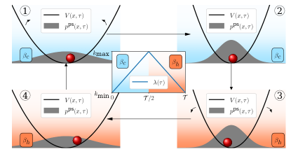
Figure 2: Particle in a harmonic trap with time-dependent stiffness $\lambda(\tau)$ operating as a Stirling heat engine between temperatures $\beta_{c}>\beta_{h}$.

The coupling to two different heat baths leads to a time-dependent temperature that is piecewise constant, i.e., $\beta(\tau)=\beta_{c}$ for $0\leq\tau<\mathcal{T}/2$ and $\beta(\tau)=\beta_{h}$ for $\mathcal{T}/2\leq\tau<\mathcal{T}$.

Currents of interest are power, entropy production and heat. Their explicit expressions and the diffusion coefficient for the output power are given in not . In order to illustrate eq. (2) and (25), we define the estimator

$$\sigma_{\mathrm{est}}\equiv\left(P_{\mathrm{out}}(\Omega)-\Omega P^{\prime}_{\mathrm{out}}(\Omega)\right)^{2}/D_{P_{\mathrm{out}}}(\Omega)\leq\sigma$$ (30)

for entropy production and vary the cycle duration $\mathcal{T}$. The output power, the estimator (30) and the bound on efficiency (25) are shown in Fig. 3.

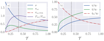
Figure 3: (a) Entropy production $\sigma$, its corresponding estimator $\sigma_{\mathrm{est}}$ (30), estimator for steady-state systems $\sigma_{\mathrm{est,TUR}}$ and output power $P_{\mathrm{out}}$ divided by its maximum $P_{\mathrm{max}}$ and (b) efficiency $\eta$, bound on the efficiency $\hat{\eta}$ (25), and its steady-state analog $\hat{\eta}_{\mathrm{ss}}$ as function of the cycle duration $\mathcal{T}$ for $\mu=10.0$, $k_{\mathrm{max}}=2.0$, $k_{\mathrm{min}}=1.0$, $\beta_{c}=2.0$ and $\beta_{h}=1.0$.

With increasing $\mathcal{T}$, the output power increases for small $\mathcal{T}$. According to eq. (2) the ordinary TUR, eq. (1), is still valid. At maximum power (vertical dotted line) eq. (2) is equivalent to the TUR and the estimator $\sigma_{\mathrm{est,TUR}}\equiv P_{\mathrm{out}}^{2}/D_{P_{\mathrm{out}}}$ intersects $\sigma_{\mathrm{est}}$. After reaching the maximum value, the power decreases with increasing $\mathcal{T}$ with the TUR violated for $\mathcal{T}\gtrsim 0.6$.

In summary, for periodically driven systems, we have derived a class of inequalities that relate, inter alia, entropy production with the mean of an observable, its dependence on driving frequency and its variance. Remarkably, apart from the more familiar currents, such observables can also be even under time-reversal like residence times are. For cyclic heat engines and cyclically driven isothermal engines, the thermodynamic efficiency can now be bounded using data only for the input or output current. Since our results have been obtained for a Markov dynamics on a discrete set of states, they trivially hold as well for overdamped Langevin dynamics. It remains an open problem whether they can be extended to underdamped dynamics. Arguably even more exciting will be to explore along similar lines periodically driven open quantum systems for which coherences are relevant.

References

- Jung (1993) P. Jung, “Periodically driven stochastic-systems,” Phys. Rep. 234, 175–295 (1993).
- Gasparinetti et al. (2014) S. Gasparinetti, P. Solinas, A. Braggio, and M. Sassetti, “Heat-exchange statistics in driven open quantum systems,” New J. Phys. 16, 115001 (2014).
- Shirai et al. (2016) Tatsuhiko Shirai, Juzar Thingna, Takashi Mori, Sergey Denisov, Peter Hänggi, and Seiji Miyashita, “Effective Floquet-Gibbs states for dissipative quantum systems,” New J. Phys. 18, 053008 (2016).
- Hartmann et al. (2017) M. Hartmann, D. Poletti, M. Ivanchenko, S. Denisov, and P. Hänggi, “Asymptotic Floquet states of open quantum systems: the role of interaction,” New J. Phys. 19, 083011 (2017).
- Restrepo et al. (2018) S. Restrepo, J. Cerrillo, P. Strasberg, and G. Schaller, “From quantum heat engines to laser cooling: Floquet theory beyond the Born-Markov approximation,” New J. Phys. 20, 053063 (2018).
- Wang et al. (2018) R. R. W. Wang, B. Xing, G. G. Carlo, and D. Poletti, “Period doubling in period-one steady states,” Phys. Rev. E 97, 020202(R) (2018).
- Gambetta et al. (2019) F. M. Gambetta, F. Carollo, M. Marcuzzi, J. P. Garrahan, and I. Lesanovsky, “Discrete time crystals in the absence of manifest symmetries or disorder in open quantum systems,” Phys. Rev. Lett. 122, 015701 (2019).
- Ciliberto (2017) S. Ciliberto, “Experiments in stochastic thermodynamics: Short history and perspectives,” Phys. Rev. X 7, 021051 (2017).
- Hayashi et al. (2012) K. Hayashi, S. de Lorenzo, M. Manosas, J. M. Huguet, and F. Ritort, “Single-molecule stochastic resonance,” Phys. Rev. X 2, 031012 (2012).
- Erbas-Cakmak et al. (2015) S. Erbas-Cakmak, D. A. Leigh, C. T. McTernan, and A. L. Nussbaumer, “Artificial molecular machines,” Chem. Rev. 115, 10081–10206 (2015).
- Schmiedl and Seifert (2008) T. Schmiedl and U. Seifert, “Efficiency at maximum power: An analytically solvable model for stochastic heat engines,” EPL 81, 20003 (2008).
- Esposito et al. (2010) M. Esposito, R. Kawai, K. Lindenberg, and C. Van den Broeck, “Quantum-dot Carnot engine at maximum power,” Phys. Rev. E 81, 041106 (2010).
- Blickle and Bechinger (2012) V. Blickle and C. Bechinger, “Realization of a micrometre-sized stochastic heat engine,” Nature Phys. 8, 143 (2012).
- Abah et al. (2012) O. Abah, J. Roßnagel, G. Jacob, S. Deffner, F. Schmidt-Kaler, K. Singer, and E. Lutz, “Single-ion heat engine at maximum power,” Phys. Rev. Lett. 109, 203006 (2012).
- Zhang et al. (2014) K. Zhang, F. Bariani, and P. Meystre, “Quantum optomechanical heat engine,” Phys. Rev. Lett. 112, 150602 (2014).
- Verley et al. (2014) Gatien Verley, Massimiliano Esposito, Tim Willaert, and Christian Van den Broeck, “The unlikely Carnot efficiency,” Nat. Commun. 5, 4721 (2014).
- Campisi et al. (2015) Michele Campisi, Jukka Pekola, and Rosario Fazio, “Nonequilibrium fluctuations in quantum heat engines: theory, example, and possible solid state experiments,” New J. Phys. 17, 035012 (2015).
- Pekola (2015) Jukka P. Pekola, “Towards quantum thermodynamics in electronic circuits,” Nature Phys. 11, 118–123 (2015).
- Uzdin et al. (2015) R. Uzdin, A. Levy, and R. Kosloff, “Equivalence of quantum heat machines, and quantum-thermodynamic signature,” Phys. Rev. X 5, 031044 (2015).
- Brandner et al. (2015) Kay Brandner, Keiji Saito, and Udo Seifert, “Thermodynamics of micro- and nano-systems driven by periodic temperature variations,” Phys. Rev. X 5, 031019 (2015).
- Roßnagel et al. (2016) J. Roßnagel, S. T. Dawkins, K. N. Tolazzi, O. Abah, E. Lutz, F. Schmidt-Kaler, and K. Singer, “A single-atom heat engine,” Science 352, 325–329 (2016).
- Kosloff and Rezek (2017) R. Kosloff and Y. Rezek, “The quantum harmonic Otto cycle,” Entropy 19, 136 (2017).
- Martinez et al. (2017) Ignacio A. Martinez, Edgar Roldan, Luis Dinis, and Raul A. Rica, “Colloidal heat engines: a review,” Soft Matter 13, 22–36 (2017).
- Barato and Seifert (2015) Andre C. Barato and Udo Seifert, “Thermodynamic uncertainty relation for biomolecular processes,” Phys. Rev. Lett. 114, 158101 (2015).
- Gingrich et al. (2016) Todd R. Gingrich, Jordan M. Horowitz, Nikolay Perunov, and Jeremy L. England, “Dissipation bounds all steady-state current fluctuations,” Phys. Rev. Lett. 116, 120601 (2016).
- Pietzonka et al. (2016a) Patrick Pietzonka, Andre C Barato, and Udo Seifert, “Universal bound on the efficiency of molecular motors,” J. Stat. Mech.: Theor. Exp. , 124004 (2016a).
- Hwang and Hyeon (2018) Wonseok Hwang and Changbong Hyeon, “Energetic costs, precision, and transport efficiency of molecular motors,” J. Phys. Chem. Lett. 9, 513–520 (2018).
- Nguyen and Vaikuntanathan (2016) Michael Nguyen and Suriyanarayanan Vaikuntanathan, “Design principles for nonequilibrium self-assembly,” Proc. Natl. Acad. Sci. U.S.A. 113, 14231–14236 (2016).
- Shiraishi et al. (2016) Naoto Shiraishi, Keiji Saito, and Hal Tasaki, “Universal trade-off relation between power and efficiency for heat engines,” Phys. Rev. Lett. 117, 190601 (2016).
- Campisi and Fazio (2016) Michele Campisi and Rosario Fazio, “The power of a critical heat engine,” Nat. Commun. 7, 11895 (2016).
- Polettini and Esposito (2017) Matteo Polettini and Massimiliano Esposito, “Carnot efficiency at divergent power output,” EPL 118, 40003 (2017).
- Pietzonka and Seifert (2018) Patrick Pietzonka and Udo Seifert, “Universal trade-off between power, efficiency and constancy in steady-state heat engines,” Phys. Rev. Lett. 120, 190602 (2018).
- Holubec and Ryabov (2018) Viktor Holubec and Artem Ryabov, “Cycling tames power fluctuations near optimum efficiency,” Phys. Rev. Lett. 121, 120601 (2018).
- Pietzonka et al. (2016b) Patrick Pietzonka, Andre C. Barato, and Udo Seifert, “Universal bounds on current fluctuations,” Phys. Rev. E 93, 052145 (2016b).
- Gingrich et al. (2017) Todd R Gingrich, Grant M Rotskoff, and Jordan M Horowitz, “Inferring dissipation from current fluctuations,” J. Phys. A: Math. Theor. 50, 184004 (2017).
- Polettini et al. (2016) Matteo Polettini, Alexandre Lazarescu, and Massimiliano Esposito, “Tightening the uncertainty principle for stochastic currents,” Phys. Rev. E 94, 052104 (2016).
- Pietzonka et al. (2017) Patrick Pietzonka, Felix Ritort, and Udo Seifert, “Finite-time generalization of the thermodynamic uncertainty relation,” Phys. Rev. E 96, 012101 (2017).
- Horowitz and Gingrich (2017) Jordan M. Horowitz and Todd R. Gingrich, “Proof of the finite-time thermodynamic uncertainty relation for steady-state currents,” Phys. Rev. E 96, 020103(R) (2017).
- Dechant and ichi Sasa (2018) Andreas Dechant and Shin ichi Sasa, “Current fluctuations and transport efficiency for general Langevin systems,” J. Stat. Mech. Theor. Exp. , 063209 (2018).
- Pigolotti et al. (2017) Simone Pigolotti, Izaak Neri, Édgar Roldán, and Frank Jülicher, “Generic properties of stochastic entropy production,” Phys. Rev. Lett. 119, 140604 (2017).
- Brandner et al. (2018) Kay Brandner, Taro Hanazato, and Keiji Saito, “Thermodynamic bounds on precision in ballistic multiterminal transport,” Phys. Rev. Lett. 120, 090601 (2018).
- Fischer et al. (2018) Lukas P. Fischer, Patrick Pietzonka, and Udo Seifert, “Large deviation function for a driven underdamped particle in a periodic potential,” Phys. Rev. E 97, 022143 (2018).
- Dechant and Sasa (2018) A. Dechant and S. I. Sasa, “Entropic bounds on currents in Langevin systems,” Phys. Rev. E 97, 062101 (2018).
- Chun et al. (2019) H.-M. Chun, L. P. Fischer, and U. Seifert, “Effect of a magnetic field on the thermodynamic uncertainty relation,” arXiv:1903.06480 (2019).
- Nardini and Touchette (2018) Cesare Nardini and Hugo Touchette, “Process interpretation of current entropic bounds,” Eur. Phys. J. B 91, 16 (2018).
- Maes (2017) Christian Maes, “Frenetic bounds on the entropy production,” Phys. Rev. Lett. 119, 160601 (2017).
- Terlizzi and Baiesi (2018) I. Terlizzi and M. Baiesi, “Kinetic uncertainty relation,” J. Phys. A 52, 02LT03 (2018).
- Gingrich and Horowitz (2017) Todd R. Gingrich and Jordan M. Horowitz, “Fundamental bounds on first passage time fluctuations for currents,” Phys. Rev. Lett. 119, 170601 (2017).
- Garrahan (2017) Juan P. Garrahan, “Simple bounds on fluctuations and uncertainty relations for first-passage times of counting observables,” Phys. Rev. E 95, 032134 (2017).
- Macieszczak et al. (2018) Katarzyna Macieszczak, Kay Brandner, and Juan P. Garrahan, “Unified thermodynamic uncertainty relations in linear response,” Phys. Rev. Lett. 121, 130601 (2018).
- Agarwalla and Segal (2018) B. K. Agarwalla and D. Segal, “Assessing the validity of the thermodynamic uncertainty relation in quantum systems,” Phys. Rev. B 98, 155438 (2018).
- Carrega et al. (2019) M. Carrega, M. Sassetti, and U. Weiss, “Optimal work-to-work conversion of a nonlinear quantum brownian duet,” arXiv:1901.10881 (2019).
- Ptaszyński (2018) K. Ptaszyński, “Coherence-enhanced constancy of a quantum thermoelectric generator,” Phys. Rev. B 98, 085425 (2018).
- Guarnieri et al. (2019) G. Guarnieri, G. T. Landi, S. R. Clark, and J. Goold, “Thermodynamics of precision in quantum non equilibrium steady states,” arXiv:1901.10428 (2019).
- Barato and Seifert (2016) Andre C. Barato and Udo Seifert, “Cost and precision of Brownian clocks,” Phys. Rev. X 6, 041053 (2016).
- Proesmans and Van den Broeck (2017) Karel Proesmans and Christian Van den Broeck, “Discrete-time thermodynamic uncertainty relation,” EPL 119, 20001 (2017).
- Barato et al. (2018a) Andre C. Barato, Raphael Chetrite, Alessandra Faggionato, and Davide Gabrielli, “Bounds on current fluctuations in periodically driven systems,” New J. Phys. 20, 103023 (2018a).
- Barato et al. (2018b) A. C. Barato, R. Chetrite, A. Faggionato, and D. Gabrielli, “A unifying picture of generalized thermodynamic uncertainty relations,” arXiv:1810.11894 (2018b).
- Koyuk et al. (2019) T. Koyuk, U. Seifert, and P. Pietzonka, “A generalization of the thermodynamic uncertainty relation to periodically driven systems,” J. Phys. A Math. Theor. 52, 02LT02 (2019).
- Rotskoff (2017) Grant M. Rotskoff, “Mapping current fluctuations of stochastic pumps to nonequilibrium steady states,” Phys. Rev. E 95, 030101(R) (2017).
- Proesmans and Horowitz (2019) K. Proesmans and J. M. Horowitz, “Hysteretic thermodynamic uncertainty relation for systems with broken time-reversal symmetry,” arXiv:1902.07008 (2019).
- Seifert (2019) Udo Seifert, “From stochastic thermodynamics to thermodynamic inference,” Ann. Rev. Cond. Mat. Phys. 10, 171–192 (2019).
- (63) See Supplemental Material at […] for details of derivations, examples, and further generalizations.